An improved upper bound for the Froude number of irrotational solitary water waves
Abstract.
A classical and central problem in the theory of water waves is to classify parameter regimes for which nontrivial solitary waves exist. In the two-dimensional, irrotational, pure gravity case, the Froude number Fr (a non-dimensional wave speed) plays the central role. So far, the best analytic result was obtained by Starr [16], while the numerical evidence of Longuet-Higgins & Fenton [12] states . On the other hand, as shown recently by Kozlov [9], the upper bound is related to the existence of subharmonic bifurcations of Stokes waves. In this paper, we develop a new strategy utilizing the flow force function and rigorously establish the improved upper bound .
1. Introduction
The mathematical theory of solitary waves has a long and well-known history going all the way back to the discovery of John Scott Russell in 1844. We refer to [15] for an overview of early works on solitary waves. A two-dimensional solitary wave is characterized by the surface profile that describes a fluid elevation localized in space. More precisely, the limits of as exist and are equal to the unperturbed depth level . Then, following [5], we define the Froude number of a traveling solitary wave as
where is the gravitational constant. It is well known that solitary waves are absent in the parameter regime ; see [16], [2], [13], and [11]. As for the upper bounds, we recall Starr [16], who derived the striking identity
Starting from here and estimating the wave amplitude from the Bernoulli equation, it is easy to obtain the upper bound . Starr immediately improves this result by showing that
| (1) |
which implies ; see [8] for another derivation. Surprisingly, the inequality has remained the best analytic result so far, although the numerical evidence from [12] (see also [14]) suggests a significantly better estimate . The question of finding an improved bound was recently re-emphasized in [9], relating it to the existence of subharmonic bifurcations of Stokes waves. Thus, the goal of this paper is to improve previous rigorous inequalities by proving the following main result.
Theorem 1.
The Froude number of any solitary wave is bounded from above by .
2. Preliminaries
In terms of non-dimensional variables as in [7], the two-dimensional, irrotational water wave problem reads
| (2a) | |||||
| (2b) | |||||
| (2c) | |||||
| (2d) | |||||
Here, the mass flux and the gravitational constant were scaled to unity. The stream function gives rise to the (relative) velocity field (in the frame co-moving with the wave). The fluid domain is , where the graph of describes the free surface . Moreover, is referred to as the Bernoulli constant. In what follows we only require to be continuous within the fluid domain up to the boundary, while the surface profile is just continuous. In particular, all our results will be valid for extreme waves.
In this paper we are concerned with solitary wave solutions of (2) that can be characterized by surface profiles such that as . In fact, any solitary wave is a wave of elevation with , while the symmetric surface profile is strictly monotonically decreasing for (and increasing for ); for more details see [4] and [11]. The crest is located at the vertical and we denote
Given any Bernoulli constant one finds two conjugate streams with depths and that are the unique roots of the
| (3) |
Note that the assumption is valid for all water waves; check [2], [6] and [10]. Thus, any solitary water wave is subject to the bounds
| (4) |
See [6] and [10] for more details. Finally, we note that the Froude number Fr can be computed as
Another important quantity, introduced in [3], is the flow force constant given by
| (5) |
here, the first expression is easily seen to be independent of , just by means of (2), while the identity follows by taking the limits . As for an upper bound for the Froude number, let us present the following simple argument which involves and leads to the inequality , and is in fact very similar to an argument in [8].
We apply (5) right below the crest (i.e., for ) and use the Cauchy-Schwarz inequality (noting that is not constant)
| (6) |
to estimate
| (7) |
A direct computation reveals that only for and . Thus, by (4) and since is decreasing for , we obtain
| (8) |
In combination with the identities (3) and (5), one immediately finds that this inequality is only true if . Furthermore, one can plug (3), (5) and into (7) to obtain Starr’s inequality (1), and that is completely avoiding any integral identities. Let us also remark that the bound yields the upper bound via (3) and (5); therefore, throughout this paper it is sufficient to consider
| (9) |
Our proof of the main theorem is based on improving the Cauchy-Schwarz inequality (6) or, equivalently, on estimating the integral
from below, where is the average of . Here, one has to consider several cases: the wave is far from stagnation, so that ; moderate distance from stagnation: for some small ; and the close to stagnation case and . Then we will numerically identify the best value of , leading to the best overall estimate for the Froude number.
3. Some lemmas
In the following, we make use of the flow force function
defined in the fluid domain and satisfying
| (10) |
Lemma 2.
For an arbitrary solution, we have
| (11) |
everywhere at the bottom.
Proof.
We consider the following harmonic function
Note that is increasing on the interval , since the derivative is zero only for but
| (12) |
this inequality follows from the definition of and its monotonicity in on the interval , which contains by (8).
Lemma 3.
The following estimate
| (13) |
holds true everywhere below the crest.
Proof.
Lemma 4.
The following estimate
| (14) |
holds true everywhere below the crest.
Proof.
To verify the result we need to show that the function
attains its minimum at the bottom, right below the crest. If so, then (14) follows directly from the definition of . Thus, we assume the contrary and the minimum of is at the surface (note that attains its minimum right below the crest). Note that , which corresponds to the upper bound for the slope obtained in [1]. This forces
at the surface and so, by the weak maximum principle,
| (15) |
In particular, we have
Now, the function cannot attain its maximum at the bottom (which would violate Hopf’s lemma), so that . Recalling (3), this implies . In its turn this forces , because otherwise we have
which requires . Finally, we use (15) to estimate
This inequality is false for all , leading to a contradiction. Thus, we have verified that the minimum of has to be attained at the bottom for all solitary waves. This finishes the proof. ∎
Now we are ready to combine the previous results presenting a proof of the main theorem.
4. A proof of Theorem 1
Below we will obtain estimates for the Froude number of arbitrary solitary wave solutions, by interpolating between three cases: when a wave is very far from, moderately far from, and close to stagnation. A slightly better estimate is found for extreme waves.
Throughout the proof, we only estimate quantities below the crest line, that is, all quantities are understood to be evaluated at .
4.1. The case
We use (7) and the monotonicity property of to find , which implies and thus . Here and in the following, we write any final inequality, which depends on , and , only in terms of by means of (3) and (5), and study the resulting inequality for – consisting only of explicit analytic expressions in – numerically.
4.2. The case and .
Here we will exploit the inequality
for reasons of computational convenience, although it is not optimal. In the next section we will obtain a slightly sharper result for waves close to stagnation based on the improved inequality (13).
First, we estimate
Here, are defined from the respective relations
note that is strictly decreasing in . For the first integral we use
| (16) |
and the Cauchy-Schwarz inequality to find
The second integral can be estimated directly as
Combining the two results, we conclude
We are interested in monotonicity of for a fixed with respect to . The plot of the corresponding derivative is shown in Figure 1. We are interested in so the ranges there are taken as
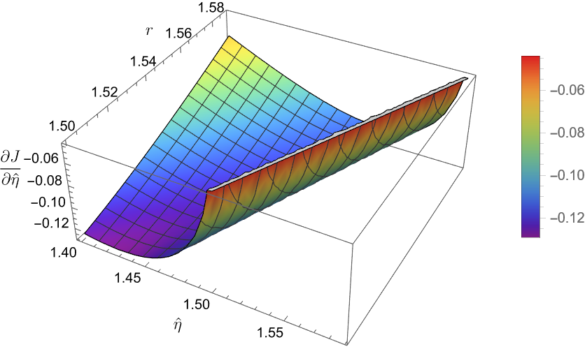
Recall that is the minimal critical value and that is slightly larger than , the value corresponding to the Froude number bound of . It is clear from Figure 1 that
within the region. The maximum there corresponds to , where
Thus, assuming and , we obtain
This inequality implies bounds for the depth and the Froude number Fr for different , see Table 1. In fact, for , so the table above can be extended further, if needed. This table can be used for estimating the Froude number of solitary waves close to but not reaching stagnation.
| (less than) | (lower bound) | Fr (upper bound) |
|---|---|---|
| 0 | 0.80719 | 1.37891 |
| 0.001 | 0.80726 | 1.37872 |
| 0.00201 | 0.80739 | 1.37838 |
| 0.005 | 0.80796 | 1.37694 |
| 0.01 | 0.80924 | 1.37368 |
| 0.05 | 0.82508 | 1.33429 |
| 0.09 | 0.84498 | 1.28744 |
We can also verify the inequality rigorously as follows:
For the inequalities above we used the bounds , and , and that for any , is strictly decreasing in .
4.3. The case and .
Let us assume , for some small . Then we can use Lemma 4 to estimate
for . We use this inequality in (13) to obtain
through (11). Now we estimate
Let be such that . First, we note that . Then, using monotonicity of , we conclude
leading to
Note that for all , while . The last inequality holds true whenever , which is granted by the assumption and the fact that (see (9)). Now let be such that . Then and so . On the other hand, we have , which is equivalent to the same inequality . And then for all . The remaining option is that there are no such root so that . But again, since , then the inequality must be true for all .
Next we write
For the first integral, recalling (16), we have
The right-hand side here is an expression of only , , and .
Similarly, we estimate as follows:
Finally, we conclude
The right-hand side here can be computed explicitly in terms of , and , but the expression is quite long to be presented. We instead study this inequality numerically and find the bounds listed in Table 2.
| (less than) | (lower bound) | Fr (upper bound) |
|---|---|---|
| 0 | 0.80866 | 1.37514 |
| 0.001 | 0.80800 | 1.37683 |
| 0.00201 | 0.80740 | 1.37837 |
We find that independently of we always get the upper bound for the Froude number of , corresponding to . This finishes the proof of the theorem.
Acknowledgments
This research was funded in whole or in part by the Austrian Science Fund (FWF) [10.55776/ESP654]. For open access purposes, the author has applied a CC BY public copyright license to any author-accepted manuscript version arising from this submission.
References
- [1] C. J. Amick, Bounds for water waves, Arch. Ration. Mech. Anal., 99 (1987), pp. 91–114.
- [2] C. J. Amick and J. F. Toland, On solitary water-waves of finite amplitude, Arch. Rational Mech. Anal., 76 (1981), pp. 9–95.
- [3] T. B. Benjamin and M. J. Lighthill, On cnoidal waves and bores, Proc. R. Soc. Lond., 224 (1954), pp. 448–460.
- [4] W. Craig and P. Sternberg, Symmetry of solitary waves, Comm. Partial Differential Equations, 13 (1988), pp. 603–633.
- [5] W. Froude, On Experiments with HMS Greyhound, Institution of Naval Architects, 1874.
- [6] G. Keady and J. Norbury, Water waves and conjugate streams, J. Fluid Mech., 70 (1975), pp. 663–671.
- [7] , On the existence theory for irrotational water waves, Math. Proc. Cambridge Philos. Soc., 83 (1978), pp. 137–157.
- [8] G. Keady and W. G. Pritchard, Bounds for surface solitary waves, Proc. Cambridge Philos. Soc., 76 (1974), pp. 345–358.
- [9] V. Kozlov, On the first bifurcation of Stokes waves, (2023). arXiv: 2307.05573.
- [10] V. Kozlov and N. Kuznetsov, Fundamental bounds for steady water waves, Math. Ann., 345 (2009), pp. 643–655.
- [11] V. Kozlov, E. Lokharu, and M. H. Wheeler, Nonexistence of subcritical solitary waves, Arch. Ration. Mech. Anal., 241 (2021), pp. 535–552.
- [12] M. S. Longuet-Higgins and J. D. Fenton, On the mass, momentum, energy and circulation of a solitary wave. II, Proc. R. Soc. Lond., 340 (1974), pp. 471–493.
- [13] J. B. McLeod, The Froude number for solitary waves, Proc. Roy. Soc. Edinburgh Sect. A, 97 (1984), pp. 193–197.
- [14] J. W. Miles, Solitary waves, Annu. Rev. Fluid Mech., 12 (1980), p. 11–43.
- [15] J. Sander and K. Hutter, On the development of the theory of the solitary wave. A historical essay, Acta Mech., 86 (1991), p. 111–152.
- [16] V. P. Starr, Momentum and energy integrals for gravity waves of finite height, J. Mar. Res., 6 (1947), pp. 175–193.