Sassha: Sharpness-aware Adaptive Second-order Optimization
with Stable Hessian Approximation

Dahun Shin    Dongyeop Lee    Jinseok Chung    Namhoon Lee
Abstract

Approximate second-order optimization methods often exhibit poorer generalization compared to first-order approaches. In this work, we look into this issue through the lens of the loss landscape and find that existing second-order methods tend to converge to sharper minima compared to SGD. In response, we propose Sassha, a novel second-order method designed to enhance generalization by explicitly reducing sharpness of the solution, while stabilizing the computation of approximate Hessians along the optimization trajectory. In fact, this sharpness minimization scheme is crafted also to accommodate lazy Hessian updates, so as to secure efficiency besides flatness. To validate its effectiveness, we conduct a wide range of standard deep learning experiments where Sassha demonstrates its outstanding generalization performance that is comparable to, and mostly better than, other methods. We provide a comprehensive set of analyses including convergence, robustness, stability, efficiency, and cost.

Machine Learning, ICML

1 Introduction

Approximate second-order methods have recently gained a surge of interest due to their potential to accelerate the large-scale training process with minimal computational and memory overhead (Yao et al., 2021; Liu et al., 2024; Gupta et al., 2018). However, studies also suggest that these methods may undermine generalization, trying to identify underlying factors behind this loss (Wilson et al., 2017; Zhou et al., 2020; Zou et al., 2022). For instance, Amari et al. (2021) shows that preconditioning hinders achieving the optimal bias for population risk, and Wadia et al. (2021) points to negative effect of whitening data.

While the precise understanding is still under investigation, many studies have suggested a strong correlation between the flatness of minima and their generalization capabilities (Keskar et al., 2017), spurring the development of optimization techniques aimed at inducing flat minima (Chaudhari et al., 2017; Izmailov et al., 2018; Foret et al., 2021; Orvieto et al., 2022). Inspired by this, we raise an important question in this work: what type of minima do second-order methods converge to, and is there any potential for improving their generalization performance based on that?

Refer to caption
Figure 1: Motivating toy example (a mixture of bivariate Gaussian densities). Sassha converges to a flat minimum unlike others.

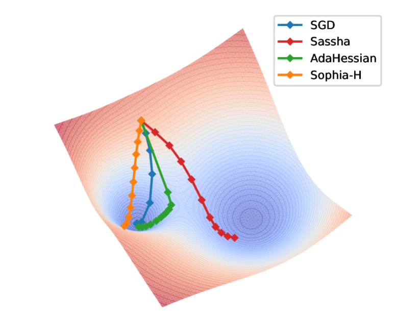
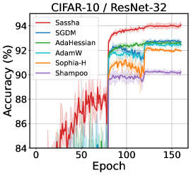
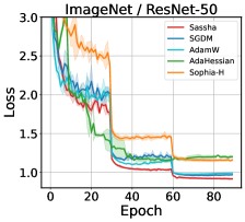
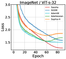
To answer these questions, we first measure the sharpness of different second-order methods using diverse metrics, suggesting that they converge to significantly sharper minima compared to stochastic gradient descent (SGD). Then, we propose SasshaSharpness-aware Adaptive Second-order optimization with Stable Hessian Approximation—designed to enhance the generalization of approximate second-order methods by explicitly reducing sharpness (see Figure˜1 for the basic results).

Sassha incorporates a sharpness minimization scheme similar to SAM (Foret et al., 2021) into the second-order optimization framework, in which the Hessian diagonal is estimated. Such estimates, however, can become numerically unstable when enforcing the sharpness reduction process. To increase stability while preserving the benefits of reduced sharpness, we make a series of well-engineered design choices based on principles studied in the literature. This not only smoothly adjusts underestimated curvature, but also enables efficient reuse of previously computed Hessians, resulting in a stable and efficient algorithm.

We extensively evaluate the effectiveness of Sassha across diverse vision and natural language tasks. Our results reveal that Sassha consistently achieves flatter minima and attains stronger generalization performance, all compared to existing practical second-order methods, and interestingly, to first-order methods including SGD, AdamW, and SAM. Furthermore, we provide an array of additional analyses to comprehensively study Sassha including convergence, robustness, stability, efficiency, and cost.

Table 1: Sharpness measurements of the solutions found by different optimizers and their generalization for ResNet-32 on CIFAR-100. Approximate second-order methods tend to yield highly sharp solutions and poor generalization compared to Sassha. We provide more results for other workloads in Appendix˜A where the same trend holds.
Sharpness Generalization
$\lambda_{max}(H)$ $\operatorname{tr}(H)_{\times 10^{3}}$ $\delta L_{\text{grad}}$ $\delta L_{\text{avg}\times 10^{-3}}$ $L_{\text{val}}$ $\text{Acc}_{\text{val}}$ (%)
SGD 265±25265_{{\color[rgb]{0.4,0.4,0.4}\definecolor[named]{pgfstrokecolor}{rgb}{0.4,0.4,0.4}\pgfsys@color@gray@stroke{0.4}\pgfsys@color@gray@fill{0.4}\pm 25}} 7.29±0.307.29_{{\color[rgb]{0.4,0.4,0.4}\definecolor[named]{pgfstrokecolor}{rgb}{0.4,0.4,0.4}\pgfsys@color@gray@stroke{0.4}\pgfsys@color@gray@fill{0.4}\pm 0.30}} 0.703±0.1320.703_{{\color[rgb]{0.4,0.4,0.4}\definecolor[named]{pgfstrokecolor}{rgb}{0.4,0.4,0.4}\pgfsys@color@gray@stroke{0.4}\pgfsys@color@gray@fill{0.4}\pm 0.132}} 1.31±1.031.31_{{\color[rgb]{0.4,0.4,0.4}\definecolor[named]{pgfstrokecolor}{rgb}{0.4,0.4,0.4}\pgfsys@color@gray@stroke{0.4}\pgfsys@color@gray@fill{0.4}\pm 1.03}} 1.260±0.0011.260_{{\color[rgb]{0.4,0.4,0.4}\definecolor[named]{pgfstrokecolor}{rgb}{0.4,0.4,0.4}\pgfsys@color@gray@stroke{0.4}\pgfsys@color@gray@fill{0.4}\pm 0.001}} 69.32±0.1969.32_{{\color[rgb]{0.4,0.4,0.4}\definecolor[named]{pgfstrokecolor}{rgb}{0.4,0.4,0.4}\pgfsys@color@gray@stroke{0.4}\pgfsys@color@gray@fill{0.4}\pm 0.19}}
Sophia-H 22797±1085722797_{{\color[rgb]{0.4,0.4,0.4}\definecolor[named]{pgfstrokecolor}{rgb}{0.4,0.4,0.4}\pgfsys@color@gray@stroke{0.4}\pgfsys@color@gray@fill{0.4}\pm 10857}} 68.15±20.1968.15_{{\color[rgb]{0.4,0.4,0.4}\definecolor[named]{pgfstrokecolor}{rgb}{0.4,0.4,0.4}\pgfsys@color@gray@stroke{0.4}\pgfsys@color@gray@fill{0.4}\pm 20.19}} 8.130±3.0828.130_{{\color[rgb]{0.4,0.4,0.4}\definecolor[named]{pgfstrokecolor}{rgb}{0.4,0.4,0.4}\pgfsys@color@gray@stroke{0.4}\pgfsys@color@gray@fill{0.4}\pm 3.082}} 19.19±6.3819.19_{{\color[rgb]{0.4,0.4,0.4}\definecolor[named]{pgfstrokecolor}{rgb}{0.4,0.4,0.4}\pgfsys@color@gray@stroke{0.4}\pgfsys@color@gray@fill{0.4}\pm 6.38}} 1.463±0.0221.463_{{\color[rgb]{0.4,0.4,0.4}\definecolor[named]{pgfstrokecolor}{rgb}{0.4,0.4,0.4}\pgfsys@color@gray@stroke{0.4}\pgfsys@color@gray@fill{0.4}\pm 0.022}} 67.76±0.3767.76_{{\color[rgb]{0.4,0.4,0.4}\definecolor[named]{pgfstrokecolor}{rgb}{0.4,0.4,0.4}\pgfsys@color@gray@stroke{0.4}\pgfsys@color@gray@fill{0.4}\pm 0.37}}
AdaHessian 11992±577911992_{{\color[rgb]{0.4,0.4,0.4}\definecolor[named]{pgfstrokecolor}{rgb}{0.4,0.4,0.4}\pgfsys@color@gray@stroke{0.4}\pgfsys@color@gray@fill{0.4}\pm 5779}} 46.94±17.6046.94_{{\color[rgb]{0.4,0.4,0.4}\definecolor[named]{pgfstrokecolor}{rgb}{0.4,0.4,0.4}\pgfsys@color@gray@stroke{0.4}\pgfsys@color@gray@fill{0.4}\pm 17.60}} 4.119±1.1364.119_{{\color[rgb]{0.4,0.4,0.4}\definecolor[named]{pgfstrokecolor}{rgb}{0.4,0.4,0.4}\pgfsys@color@gray@stroke{0.4}\pgfsys@color@gray@fill{0.4}\pm 1.136}} 12.50±6.0812.50_{{\color[rgb]{0.4,0.4,0.4}\definecolor[named]{pgfstrokecolor}{rgb}{0.4,0.4,0.4}\pgfsys@color@gray@stroke{0.4}\pgfsys@color@gray@fill{0.4}\pm 6.08}} 1.377±0.0701.377_{{\color[rgb]{0.4,0.4,0.4}\definecolor[named]{pgfstrokecolor}{rgb}{0.4,0.4,0.4}\pgfsys@color@gray@stroke{0.4}\pgfsys@color@gray@fill{0.4}\pm 0.070}} 68.06±0.2268.06_{{\color[rgb]{0.4,0.4,0.4}\definecolor[named]{pgfstrokecolor}{rgb}{0.4,0.4,0.4}\pgfsys@color@gray@stroke{0.4}\pgfsys@color@gray@fill{0.4}\pm 0.22}}
Shampoo 436374±9017436374_{{\color[rgb]{0.4,0.4,0.4}\definecolor[named]{pgfstrokecolor}{rgb}{0.4,0.4,0.4}\pgfsys@color@gray@stroke{0.4}\pgfsys@color@gray@fill{0.4}\pm 9017}} 6823.34±664.656823.34_{{\color[rgb]{0.4,0.4,0.4}\definecolor[named]{pgfstrokecolor}{rgb}{0.4,0.4,0.4}\pgfsys@color@gray@stroke{0.4}\pgfsys@color@gray@fill{0.4}\pm 664.65}} 73.27±12.5173.27_{{\color[rgb]{0.4,0.4,0.4}\definecolor[named]{pgfstrokecolor}{rgb}{0.4,0.4,0.4}\pgfsys@color@gray@stroke{0.4}\pgfsys@color@gray@fill{0.4}\pm 12.51}} 49307489±5697979449307489_{{\color[rgb]{0.4,0.4,0.4}\definecolor[named]{pgfstrokecolor}{rgb}{0.4,0.4,0.4}\pgfsys@color@gray@stroke{0.4}\pgfsys@color@gray@fill{0.4}\pm 56979794}} 1.386±0.0101.386_{{\color[rgb]{0.4,0.4,0.4}\definecolor[named]{pgfstrokecolor}{rgb}{0.4,0.4,0.4}\pgfsys@color@gray@stroke{0.4}\pgfsys@color@gray@fill{0.4}\pm 0.010}} 64.08±0.4664.08_{{\color[rgb]{0.4,0.4,0.4}\definecolor[named]{pgfstrokecolor}{rgb}{0.4,0.4,0.4}\pgfsys@color@gray@stroke{0.4}\pgfsys@color@gray@fill{0.4}\pm 0.46}}
Sassha 107±40\textbf{107}_{{\color[rgb]{0.4,0.4,0.4}\definecolor[named]{pgfstrokecolor}{rgb}{0.4,0.4,0.4}\pgfsys@color@gray@stroke{0.4}\pgfsys@color@gray@fill{0.4}\pm 40}} 1.87±0.65\textbf{1.87}_{{\color[rgb]{0.4,0.4,0.4}\definecolor[named]{pgfstrokecolor}{rgb}{0.4,0.4,0.4}\pgfsys@color@gray@stroke{0.4}\pgfsys@color@gray@fill{0.4}\pm 0.65}} 0.238±0.088\textbf{0.238}_{{\color[rgb]{0.4,0.4,0.4}\definecolor[named]{pgfstrokecolor}{rgb}{0.4,0.4,0.4}\pgfsys@color@gray@stroke{0.4}\pgfsys@color@gray@fill{0.4}\pm 0.088}} 0.65±0.86\textbf{0.65}_{{\color[rgb]{0.4,0.4,0.4}\definecolor[named]{pgfstrokecolor}{rgb}{0.4,0.4,0.4}\pgfsys@color@gray@stroke{0.4}\pgfsys@color@gray@fill{0.4}\pm 0.86}} 0.961±0.005\textbf{0.961}_{{\color[rgb]{0.4,0.4,0.4}\definecolor[named]{pgfstrokecolor}{rgb}{0.4,0.4,0.4}\pgfsys@color@gray@stroke{0.4}\pgfsys@color@gray@fill{0.4}\pm 0.005}} 72.14±0.16\textbf{72.14}_{{\color[rgb]{0.4,0.4,0.4}\definecolor[named]{pgfstrokecolor}{rgb}{0.4,0.4,0.4}\pgfsys@color@gray@stroke{0.4}\pgfsys@color@gray@fill{0.4}\pm 0.16}}
Refer to caption
(a) AdaHessian
Refer to caption
(b) Sophia-H
Refer to caption
(c) Shampoo
Refer to caption
(d) Sassha
Figure 2: Visualization of the found solutions along the directions of the dominant eigenvectors.

2 Related Works

Second-order optimization for deep learning.

First-order methods such as SGD are popular optimization methods for deep learning due to their low per-iteration cost and good generalization performance (Hardt et al., 2016). However, these methods have two major drawbacks: slow convergence under ill-conditioned landscapes and high sensitivity to hyperparameter choices such as learning rate (Demeniconi & Chawla, 2020). Adaptive methods (Duchi et al., 2011; Hinton et al., 2012; Kingma & Ba, 2015) propose using empirical Fisher-type preconditioning to alleviate these issues, though recent studies suggest their insufficiency to do so (Kunstner et al., 2019). This has led to recent interest in developing approximate second-order methods such as Hessian-Free Inexact Newton methods (Martens et al., 2010; Kiros, 2013), stochastic quasi-Newton methods (Byrd et al., 2016; Gower et al., 2016), Gauss-Newton methods (Schraudolph, 2002; Botev et al., 2017), natural gradient methods (Amari et al., 2000), and Kronecker-factored approximations (Martens & Grosse, 2015; Goldfarb et al., 2020). However, these approaches still incur non-trivial memory and computational costs, or are difficult to parallelize, limiting their applicability to large-scale problems such as deep learning. This has driven growing interest in developing more scalable and efficient second-order approaches, particularly through diagonal scaling methods (Bottou et al., 2018; Yao et al., 2021; Liu et al., 2024), to better accommodate large-scale deep learning scenarios.

Sharpness minimization for generalization.

The relationship between the geometry of the loss landscape and the generalization ability of neural networks was first discussed in the work of Hochreiter & Schmidhuber (1994), and the interest in this subject has persisted over time. Expanding on this foundation, subsequent studies have explored the impact of flat regions on generalization both empirically and theoretically (Hochreiter & Schmidhuber, 1997; Keskar et al., 2017; Dziugaite & Roy, 2017; Neyshabur et al., 2017; Dinh et al., 2017; Jiang et al., 2020). Motivated by this, various approaches have been proposed to achieve flat minima such as regularizing local entropy (Chaudhari et al., 2017), averaging model weights (Izmailov et al., 2018), explicitly regularizing sharpness by solving a min-max problem (Foret et al., 2021), and injecting anti-correlated noise (Orvieto et al., 2022), to name a few. In particular, the sharpness-aware minimization (SAM) (Foret et al., 2021) has attracted significant attention for its strong generalization performance across various domains (Chen et al., 2022; Bahri et al., 2022; Qu et al., 2022) and its robustness to label noise (Baek et al., 2024). Nevertheless, to our knowledge, the sharpness minimization scheme has not been studied to enable second-order methods to find flat minima as of yet.

3 Practical Second-order Optimizers Converge to Sharp Minima

In this section, we investigate the sharpness of minima obtained by approximate second-order methods and their generalization properties. We posit that poor generalization of second-order methods reported in the literature (Amari et al., 2021; Wadia et al., 2021) can potentially be attributed to sharpness of their solutions.

We employ four metrics frequently used in the literature: maximum eigenvalue of the Hessian, the trace of Hessian, gradient-direction sharpness, and average sharpness (Hochreiter & Schmidhuber, 1997; Jastrzębski et al., 2018; Xie et al., 2020; Du et al., 2022b; Chen et al., 2022). The first two, denoted as $\lambda_{\max}(H)$ and $\operatorname{tr}(H)$, are often used as standard mathematical measures for the worst-case and the average curvature computed using the power iteration method and the Hutchinson trace estimation, respectively. The other two measures, $\delta L_{\text{grad}}$ and $\delta L_{\text{avg}}$, assess sharpness based on the loss difference under perturbations. $\delta L_{\text{grad}}$ evaluates sharpness in the gradient direction and is computed as $L(x^{\star}+\rho\nabla L(x^{\star})/\|\nabla L(x^{\star})\|)-L(x^{\star})$. $\delta L_{\text{avg}}$ computes the average loss difference over Gaussian random perturbations, expressed as $\mathbb{E}_{z\sim\mathcal{N}(0,1)}[L(x^{\star}+\rho z/\|z\|)-L(x^{\star})]$. Here we choose $\rho=0.1$ for the scale of the perturbation.

With these, we measure the sharpness of the minima found by three approximate second-order methods designed for deep learning; Sophia-H (Liu et al., 2024), AdaHessian (Yao et al., 2021), and Shampoo (Gupta et al., 2018), and compare them with Sassha as well as SGD for reference. We also compute the validation loss and accuracy to see any correlation between sharpness and generalization of these solutions. The results are presented in Table˜1.

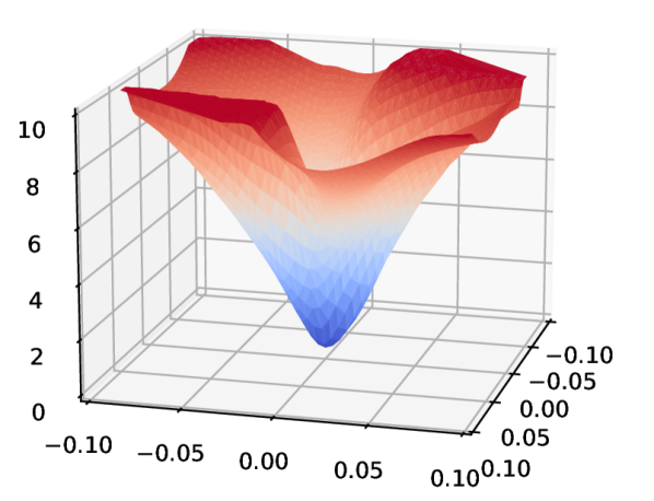
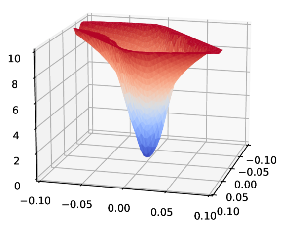
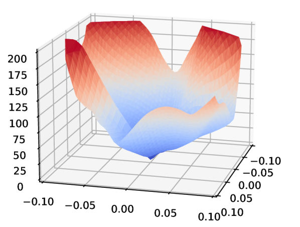
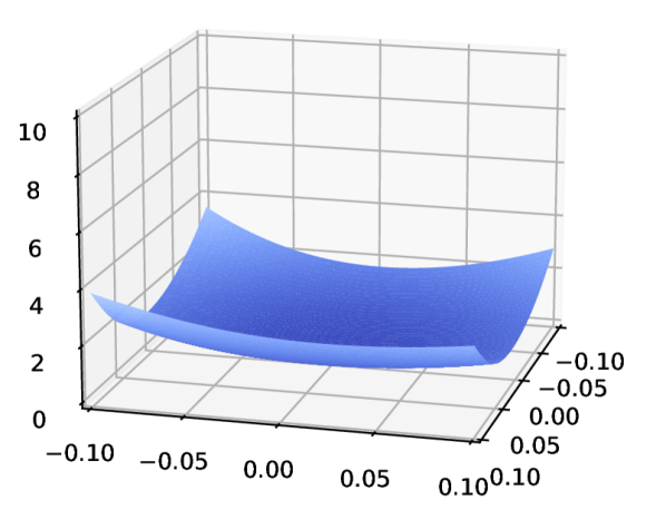
We observe that existing second-order optimizers produce solutions with significantly higher sharpness compared to Sassha in all sharpness metrics, which also correlates well with their generalization. We also provide a visualization of the loss landscape for the found solutions, where we find that the solutions obtained by second-order methods are indeed much sharper than that of Sassha (Figure˜2).

4 Method

In the previous section, we observe that the generalization performance of approximate second-order algorithms anti-correlates with the sharpness of their solutions. Based on this, we introduce Sassha—a novel adaptive second-order method designed to improve generalization by reducing sharpness without adversely impacting the Hessian.

4.1 Sharpness-aware Second-order Optimization

We consider a min-max problem, similar to Keskar et al. (2017); Foret et al. (2021), to minimize sharpness. This is defined as minimizing the objective $f$ within the entire $\rho$-ball neighborhood:

$$\min_{x\in\mathbb{R}^{d}}\max_{\|\epsilon\|_{2}\leq\rho}f(x+\epsilon),$$ (1)

Based on this, we construct our sharpness minimization technique for second-order optimization as follows. We first follow a similar procedure as Foret et al. (2021) by solving for $\epsilon$ on the first-order approximation of the objective, which exactly solves the dual norm problem as follows:

$\displaystyle\epsilon_{t}^{\star}=\mathop{\rm arg\,max}_{\|\epsilon\|_{2}\leq\rho}f(x_{t})+\epsilon^{\top}\nabla f(x_{t})$ $\displaystyle=\rho\frac{\nabla f(x_{t})}{\|\nabla f(x_{t})\|_{2}}.$ (2)

We plug this back to yield the following perturbed objective function:

$$\tilde{f}_{t}(x)\coloneqq f\left(x+\rho\frac{\nabla f(x_{t})}{\|\nabla f(x_{t})\|_{2}}\right),$$

which shifts the point of the approximately highest function value within the neighborhood to the current iterate.

With this sharpness-penalized objective, we proceed to make a second-order Taylor approximation:

$\displaystyle x_{t+1}=\mathop{\rm arg\,min}_{x}~$ $\displaystyle\tilde{f}_{t}\left(x_{t}\right)+\nabla\tilde{f}_{t}\left(x_{t}\right)^{\top}(x-x_{t})$
$\displaystyle+(x-x_{t})^{\top}\tilde{H}_{t}\left(x_{t}\right)(x-x_{t}),$

where $\tilde{H}_{t}$ denotes the Hessian of $\tilde{f}_{t}$. Using the first-order optimality condition, we derive the basis update rule for our sharpness-aware second-order optimization:

$\displaystyle x_{t+1}$ $\displaystyle=x_{t}-\tilde{H}_{t}\left(x_{t}\right)^{-1}\nabla\tilde{f}_{t}\left(x_{t}\right)$
$\displaystyle=x_{t}-H\left(x_{t}+\epsilon_{t}^{\star}\right)^{-1}\nabla f\left(x_{t}+\epsilon_{t}^{\star}\right),$

where $H$ denotes the Hessian of the original objective $f$.

Practical second-order methods must rely on approximately estimated Hessians (i.e., $H\rightarrow\widehat{H}$) since the exact computation is prohibitively expensive for large-scale problems. We choose to employ the diagonal approximation via Hutchinson’s method. However, as we will show in our analysis (Section˜6.2), we find that these estimates can become numerically unstable during the sharpness reduction process, as it penalizes Hessian entries close to zero. This can lead to fatal underestimation of the diagonal Hessian compared to scenarios without sharpness minimization, significantly disrupting training. We propose a stable Hessian approximation to address these issue in the following sections.

4.2 Improving Stability

Alleviating divergence.

Approximate second-order methods can yield overly large steps when their diagonal Hessian estimations underestimate the curvature (Dauphin et al., 2015). However, this instability seems to be more present under sharpness minimization, presumably due to smaller top Hessian eigenvalue $\lambda_{1}$ (Agarwala & Dauphin, 2023; Shin et al., 2024) yielding smaller estimated diagonal entries on average:

$$\mathbb{E}\left[\frac{1}{d}\sum_{i=1}^{d}{\widehat{H}_{ii}}\right]=\frac{1}{d}\sum_{i=1}^{d}{\mathbb{E}[\widehat{H}]_{ii}}=\frac{\operatorname{tr}(H)}{d}=\frac{1}{d}\sum_{i=1}^{d}{\lambda_{i}}\leq\lambda_{1}.$$

This tendency toward zero intensifies numerical instability during Hessian inversion, increasing the risk of training failures.

Conventional techniques such as damping or clipping can be employed to mitigate this, although their additional hyperparameters require careful tuning. Instead, we propose square rooting the Hessian (i.e., $|\widehat{H}|^{1/2}$), which effectively mitigates instability, allowing improved generalization performance over other alternatives without additional hyperparameters. We present empirical validation of this in Section˜6.2 and Section˜E.1.

Its benefits can be understood from two perspectives. First, the square root smoothly increase the magnitude of the near-zero diagonal Hessian entries in the denominator (i.e., $h<\sqrt{h}$ if $0<h<1$) while damping and clipping either shift the entire Hessian estimate or abruptly replace its certain entries to a predefined constant, potentially leading to performance degradation without careful tuning. Alternatively, it can be interpreted as a geometric interpolation between the identity matrix and the preconditioning matrix $H^{\alpha}I^{1-\alpha}$, which has been demonstrated to allow balancing between the bias and the variance of the population risk, thereby improving generalization (Amari et al., 2021). We specifically adopt $\alpha=1/2$ (i.e., square root), as it has consistently demonstrated robust performance across various scenarios (Amari et al., 2021; Kingma & Ba, 2015).

Absolute Hessian scaling

In neural network training, the computed Hessian often contains negative entries. However, since the square-root operation we introduced applies only to positive values, these entries must first be transformed. To tackle this, we attend to the prior works of Becker et al. (1988); Yao et al. (2021) and employ the absolute function to adjust the negative entries of the diagonal Hessian to be positive, i.e.

$$\lvert\widehat{H}\rvert:=\sum_{i=1}^{d}\lvert\widehat{H}_{ii}\rvert\mathbf{e}_{i}\mathbf{e}_{i}^{\top}$$ (3)

where $\widehat{H}_{ii}$ and $\mathbf{e}_{i}$ are the $i^{\text{th}}$ diagonal entry of the approximate diagonal Hessian and the $i^{\text{th}}$ standard basis vector, respectively. Importantly, this also preserve the same optimal rescaling as Newton’s method, which can provide a more effective second-order step compared to alternatives like clipping (Nocedal & Wright, 1999; Murray, 2010; Dauphin et al., 2014; Wang et al., 2013). Additionally, this transformation mitigates the risk of convergence to critical points such as saddle or local maxima. We empirically validate the effectiveness of this approach in Appendix˜H and Section˜E.2.

4.3 Improving Efficiency via Lazy Hessian Update

While the diagonal Hessian approximation can significantly reduce computations, it still requires at least twice as much backpropagation compared to first-order methods. Here we attempt to further alleviate this by lazily computing the Hessian every $k$ steps:

$$D_{t}=\begin{cases}\beta_{2}D_{t-1}+(1-\beta_{2})\lvert\widehat{H}(x_{t}+\epsilon^{\star}_{t})\rvert&\texttt{if }t\ \operatorname{mod}\ k=1\\ D_{t-1}&\texttt{otherwise}\end{cases},$$

where $D_{t}$ and $\beta_{2}$ are the moving average of the Hessian and its hyperparameter, respectively. This reduces the overhead from additional Hessian computation by $1/k$. We set $k=10$ for all experiments in this work unless stated otherwise.

However, extensive Hessian reusing will lead to significant performance degradation since it would no longer accurately reflect the current curvature (Doikov et al., 2023). Interestingly, Sassha is quite resilient against prolonged reusing, keeping its performance relatively high over longer Hessian reusing compared to other approximate second-order methods. Our investigation reveals that along the trajectory of Sassha, the Hessian tends to change less frequently than existing alternatives. We hypothesize that the introduction of sharpness minimization plays an integral role in this phenomenon by biasing the optimization path toward regions with lower curvature change, allowing the prior Hessian to remain relevant over more extended steps. We provide a detailed analysis of the lazy Hessian updates in Section˜6.3.

4.4 Algorithm

The exact steps of Sassha is outlined in Algorithm˜1. We also compare Sassha with other adaptive and second-order methods in detail in Appendix˜B, where one can see the exact differences between these sophisticated methods.

Algorithm 1 Sassha algorithm
1:  Input: Initial parameter $x_{0}$, learning rate $\{\eta_{\mathnormal{t}}\}$, moving average parameters $\beta_{1},\beta_{2}$, Hessian update interval $k$, weight decay parameter $\lambda$
2:  Set $\mathnormal{m}_{-1}=0$, $D_{-1}=0$
3:  for $\mathnormal{t}=1$ to $T$ do
4:  $\mathnormal{g}_{\mathnormal{t}}=\nabla f_{\mathcal{B}}(x_{t})$
5:  $\epsilon^{\star}_{t}=\rho g_{t}/\|g_{t}\|_{2}$
6:  $\tilde{g}_{t}=\nabla f_{\mathcal{B}}(x_{t}+\epsilon^{\star}_{t})$
7:  $m_{t}=\beta_{1}m_{t-1}+(1-\beta_{1})\tilde{g}_{t}$
8:  $\overline{m}_{t}=m_{t}/(1-\beta_{1}^{t})$
9:  if $t\operatorname{mod}k=1$ then
10:   $\tilde{H}_{t}=\widehat{H}(x_{t}+\epsilon^{\star}_{t})$ $\triangleright$ Section˜4.1
11:   $D_{\mathnormal{t}}=\beta_{2}D_{t-1}+(1-\beta_{2})|\tilde{H}_{t}|$
12:   $\overline{D}_{t}=\sqrt{D_{t}/(1-\beta_{2}^{t})}$ $\triangleright$ Section˜4.2
13:  else
14:   $\overline{D}_{t}=\overline{D}_{t-1}$ $\triangleright$ Section˜4.3
15:  end if
16:  $x_{t+1}=x_{t}-\eta_{t}\overline{D}_{t}^{-1}\overline{m}_{t}-\eta_{t}\lambda x_{t}$
17:  end for

4.5 Convergence Analysis

In this section, we present a standard convergence analysis of Sassha under the following assumptions.

Assumption 4.1.

The function $f$ is bounded from below, i.e., $f^{*}:=\inf_{x}f(x)>-\infty$.

Assumption 4.2.

The function $f$ is twice differentiable, convex, and $\beta$-smooth. That is, $0\preceq\nabla^{2}f\preceq\beta.$

Assumption 4.3.

The gradient $\nabla f(x_{t})$ is nonzero for a finite number of iterations, i.e., $\nabla f(x_{t})\neq 0$ for all $t\in\{1,2,\dots,n\}$.

Under these assumptions, we derive a descent inequality for $f(x_{t})$ by leveraging Adam-like proof techniques from Li et al. (2023) to handle the diagonal Hessian and employing smoothness-based bounds to account for the perturbation step based on analyses of Khanh et al. (2024). Now we give the convergence results as follows:

Theorem 4.4.

Under Assumptions 4.1-4.3, given any initial point $x_{0}\in\mathbb{R}^{d}$, let $\{x_{t}\}$ be generated by the update rule Sassha Equation˜5 with step sizes $\eta_{t}$ and perturbation radii $\rho_{t}$ satisfying $\sum_{t=1}^{\infty}\eta_{t}=\infty,\quad\sum_{t=1}^{\infty}\eta_{t}^{2}<\infty,\quad\sum_{t=1}^{\infty}\rho_{t}^{2}\eta_{t}<\infty$. Then, we have $\liminf_{t\to\infty}\|\nabla f(x_{t})\|=0$.

This preliminary result indicates that any limit point of Sassha is a stationary point of $f$, ensuring progress towards optimal solutions. We refer to Appendix˜C for the full proof details.

5 Evaluations

In this section, we demonstrate that Sassha can indeed improve upon existing second-order methods available for standard deep learning tasks. We also show that Sassha performs competitively to the first-order baseline methods. Specifically, Sassha is compared to AdaHessian (Yao et al., 2021), Sophia-H (Liu et al., 2024), Shampoo (Gupta et al., 2018), SGD, AdamW (Loshchilov & Hutter, 2018), and SAM (Foret et al., 2021) on a diverse set of both vision and language tasks. We emphasize that we perform an extensive hyperparameter search to rigorously tune all optimizers and ensure fair comparisons. We provide the details of experiment settings to reproduce our results in Appendix˜D. The code to reproduce all results reported in this work is made available for download at https://github.com/LOG-postech/Sassha.

5.1 Image Classification

Table 2: Image classification results of various optimization methods in terms of final validation accuracy (mean$\pm$std). Sassha consistently outperforms the other methods for all workloads. * means omitted due to excessive computational requirements.
CIFAR-10 CIFAR-100 ImageNet
Category Method ResNet-20 ResNet-32 ResNet-32 WRN-28-10 ResNet-50 ViT-s-32
First-order SGD 92.03±0.3292.03_{{\color[rgb]{0.4,0.4,0.4}\definecolor[named]{pgfstrokecolor}{rgb}{0.4,0.4,0.4}\pgfsys@color@gray@stroke{0.4}\pgfsys@color@gray@fill{0.4}\pm 0.32}} 92.69±0.0692.69_{{\color[rgb]{0.4,0.4,0.4}\definecolor[named]{pgfstrokecolor}{rgb}{0.4,0.4,0.4}\pgfsys@color@gray@stroke{0.4}\pgfsys@color@gray@fill{0.4}\pm 0.06}} 69.32±0.1969.32_{{\color[rgb]{0.4,0.4,0.4}\definecolor[named]{pgfstrokecolor}{rgb}{0.4,0.4,0.4}\pgfsys@color@gray@stroke{0.4}\pgfsys@color@gray@fill{0.4}\pm 0.19}} 80.06±0.1580.06_{{\color[rgb]{0.4,0.4,0.4}\definecolor[named]{pgfstrokecolor}{rgb}{0.4,0.4,0.4}\pgfsys@color@gray@stroke{0.4}\pgfsys@color@gray@fill{0.4}\pm 0.15}} 75.58±0.0575.58_{{\color[rgb]{0.4,0.4,0.4}\definecolor[named]{pgfstrokecolor}{rgb}{0.4,0.4,0.4}\pgfsys@color@gray@stroke{0.4}\pgfsys@color@gray@fill{0.4}\pm 0.05}} 62.90±0.3662.90_{{\color[rgb]{0.4,0.4,0.4}\definecolor[named]{pgfstrokecolor}{rgb}{0.4,0.4,0.4}\pgfsys@color@gray@stroke{0.4}\pgfsys@color@gray@fill{0.4}\pm 0.36}}
AdamW 92.04±0.1192.04_{{\color[rgb]{0.4,0.4,0.4}\definecolor[named]{pgfstrokecolor}{rgb}{0.4,0.4,0.4}\pgfsys@color@gray@stroke{0.4}\pgfsys@color@gray@fill{0.4}\pm 0.11}} 92.42±0.1392.42_{{\color[rgb]{0.4,0.4,0.4}\definecolor[named]{pgfstrokecolor}{rgb}{0.4,0.4,0.4}\pgfsys@color@gray@stroke{0.4}\pgfsys@color@gray@fill{0.4}\pm 0.13}} 68.78±0.2268.78_{{\color[rgb]{0.4,0.4,0.4}\definecolor[named]{pgfstrokecolor}{rgb}{0.4,0.4,0.4}\pgfsys@color@gray@stroke{0.4}\pgfsys@color@gray@fill{0.4}\pm 0.22}} 79.09±0.3579.09_{{\color[rgb]{0.4,0.4,0.4}\definecolor[named]{pgfstrokecolor}{rgb}{0.4,0.4,0.4}\pgfsys@color@gray@stroke{0.4}\pgfsys@color@gray@fill{0.4}\pm 0.35}} 75.38±0.0875.38_{{\color[rgb]{0.4,0.4,0.4}\definecolor[named]{pgfstrokecolor}{rgb}{0.4,0.4,0.4}\pgfsys@color@gray@stroke{0.4}\pgfsys@color@gray@fill{0.4}\pm 0.08}} 66.46±0.1566.46_{{\color[rgb]{0.4,0.4,0.4}\definecolor[named]{pgfstrokecolor}{rgb}{0.4,0.4,0.4}\pgfsys@color@gray@stroke{0.4}\pgfsys@color@gray@fill{0.4}\pm 0.15}}
SAM ${}_{\text{SGD}}$ 92.85±0.0792.85_{{\color[rgb]{0.4,0.4,0.4}\definecolor[named]{pgfstrokecolor}{rgb}{0.4,0.4,0.4}\pgfsys@color@gray@stroke{0.4}\pgfsys@color@gray@fill{0.4}\pm 0.07}} 93.89±0.1393.89_{{\color[rgb]{0.4,0.4,0.4}\definecolor[named]{pgfstrokecolor}{rgb}{0.4,0.4,0.4}\pgfsys@color@gray@stroke{0.4}\pgfsys@color@gray@fill{0.4}\pm 0.13}} 71.99±0.2071.99_{{\color[rgb]{0.4,0.4,0.4}\definecolor[named]{pgfstrokecolor}{rgb}{0.4,0.4,0.4}\pgfsys@color@gray@stroke{0.4}\pgfsys@color@gray@fill{0.4}\pm 0.20}} 83.14±0.1383.14_{{\color[rgb]{0.4,0.4,0.4}\definecolor[named]{pgfstrokecolor}{rgb}{0.4,0.4,0.4}\pgfsys@color@gray@stroke{0.4}\pgfsys@color@gray@fill{0.4}\pm 0.13}} 76.36±0.1676.36_{{\color[rgb]{0.4,0.4,0.4}\definecolor[named]{pgfstrokecolor}{rgb}{0.4,0.4,0.4}\pgfsys@color@gray@stroke{0.4}\pgfsys@color@gray@fill{0.4}\pm 0.16}} 64.54±0.6364.54_{{\color[rgb]{0.4,0.4,0.4}\definecolor[named]{pgfstrokecolor}{rgb}{0.4,0.4,0.4}\pgfsys@color@gray@stroke{0.4}\pgfsys@color@gray@fill{0.4}\pm 0.63}}
SAM ${}_{\text{AdamW}}$ 92.77±0.2992.77_{{\color[rgb]{0.4,0.4,0.4}\definecolor[named]{pgfstrokecolor}{rgb}{0.4,0.4,0.4}\pgfsys@color@gray@stroke{0.4}\pgfsys@color@gray@fill{0.4}\pm 0.29}} 93.45±0.2493.45_{{\color[rgb]{0.4,0.4,0.4}\definecolor[named]{pgfstrokecolor}{rgb}{0.4,0.4,0.4}\pgfsys@color@gray@stroke{0.4}\pgfsys@color@gray@fill{0.4}\pm 0.24}} 71.15±0.3771.15_{{\color[rgb]{0.4,0.4,0.4}\definecolor[named]{pgfstrokecolor}{rgb}{0.4,0.4,0.4}\pgfsys@color@gray@stroke{0.4}\pgfsys@color@gray@fill{0.4}\pm 0.37}} 82.88±0.3182.88_{{\color[rgb]{0.4,0.4,0.4}\definecolor[named]{pgfstrokecolor}{rgb}{0.4,0.4,0.4}\pgfsys@color@gray@stroke{0.4}\pgfsys@color@gray@fill{0.4}\pm 0.31}} 76.35±0.1676.35_{{\color[rgb]{0.4,0.4,0.4}\definecolor[named]{pgfstrokecolor}{rgb}{0.4,0.4,0.4}\pgfsys@color@gray@stroke{0.4}\pgfsys@color@gray@fill{0.4}\pm 0.16}} 68.31±0.1768.31_{{\color[rgb]{0.4,0.4,0.4}\definecolor[named]{pgfstrokecolor}{rgb}{0.4,0.4,0.4}\pgfsys@color@gray@stroke{0.4}\pgfsys@color@gray@fill{0.4}\pm 0.17}}
Second-order AdaHessian 92.00±0.1792.00_{{\color[rgb]{0.4,0.4,0.4}\definecolor[named]{pgfstrokecolor}{rgb}{0.4,0.4,0.4}\pgfsys@color@gray@stroke{0.4}\pgfsys@color@gray@fill{0.4}\pm 0.17}} 92.48±0.1592.48_{{\color[rgb]{0.4,0.4,0.4}\definecolor[named]{pgfstrokecolor}{rgb}{0.4,0.4,0.4}\pgfsys@color@gray@stroke{0.4}\pgfsys@color@gray@fill{0.4}\pm 0.15}} 68.06±0.2268.06_{{\color[rgb]{0.4,0.4,0.4}\definecolor[named]{pgfstrokecolor}{rgb}{0.4,0.4,0.4}\pgfsys@color@gray@stroke{0.4}\pgfsys@color@gray@fill{0.4}\pm 0.22}} 76.92±0.2676.92_{{\color[rgb]{0.4,0.4,0.4}\definecolor[named]{pgfstrokecolor}{rgb}{0.4,0.4,0.4}\pgfsys@color@gray@stroke{0.4}\pgfsys@color@gray@fill{0.4}\pm 0.26}} 73.64±0.1673.64_{{\color[rgb]{0.4,0.4,0.4}\definecolor[named]{pgfstrokecolor}{rgb}{0.4,0.4,0.4}\pgfsys@color@gray@stroke{0.4}\pgfsys@color@gray@fill{0.4}\pm 0.16}} 66.42±0.2366.42_{{\color[rgb]{0.4,0.4,0.4}\definecolor[named]{pgfstrokecolor}{rgb}{0.4,0.4,0.4}\pgfsys@color@gray@stroke{0.4}\pgfsys@color@gray@fill{0.4}\pm 0.23}}
Sophia-H 91.81±0.2791.81_{{\color[rgb]{0.4,0.4,0.4}\definecolor[named]{pgfstrokecolor}{rgb}{0.4,0.4,0.4}\pgfsys@color@gray@stroke{0.4}\pgfsys@color@gray@fill{0.4}\pm 0.27}} 91.99±0.0891.99_{{\color[rgb]{0.4,0.4,0.4}\definecolor[named]{pgfstrokecolor}{rgb}{0.4,0.4,0.4}\pgfsys@color@gray@stroke{0.4}\pgfsys@color@gray@fill{0.4}\pm 0.08}} 67.76±0.3767.76_{{\color[rgb]{0.4,0.4,0.4}\definecolor[named]{pgfstrokecolor}{rgb}{0.4,0.4,0.4}\pgfsys@color@gray@stroke{0.4}\pgfsys@color@gray@fill{0.4}\pm 0.37}} 79.35±0.2479.35_{{\color[rgb]{0.4,0.4,0.4}\definecolor[named]{pgfstrokecolor}{rgb}{0.4,0.4,0.4}\pgfsys@color@gray@stroke{0.4}\pgfsys@color@gray@fill{0.4}\pm 0.24}} 72.06±0.4972.06_{{\color[rgb]{0.4,0.4,0.4}\definecolor[named]{pgfstrokecolor}{rgb}{0.4,0.4,0.4}\pgfsys@color@gray@stroke{0.4}\pgfsys@color@gray@fill{0.4}\pm 0.49}} 62.44±0.3662.44_{{\color[rgb]{0.4,0.4,0.4}\definecolor[named]{pgfstrokecolor}{rgb}{0.4,0.4,0.4}\pgfsys@color@gray@stroke{0.4}\pgfsys@color@gray@fill{0.4}\pm 0.36}}
Shampoo 88.55±0.8388.55_{{\color[rgb]{0.4,0.4,0.4}\definecolor[named]{pgfstrokecolor}{rgb}{0.4,0.4,0.4}\pgfsys@color@gray@stroke{0.4}\pgfsys@color@gray@fill{0.4}\pm 0.83}} 90.23±0.2490.23_{{\color[rgb]{0.4,0.4,0.4}\definecolor[named]{pgfstrokecolor}{rgb}{0.4,0.4,0.4}\pgfsys@color@gray@stroke{0.4}\pgfsys@color@gray@fill{0.4}\pm 0.24}} 64.08±0.4664.08_{{\color[rgb]{0.4,0.4,0.4}\definecolor[named]{pgfstrokecolor}{rgb}{0.4,0.4,0.4}\pgfsys@color@gray@stroke{0.4}\pgfsys@color@gray@fill{0.4}\pm 0.46}} 74.06±1.2874.06_{{\color[rgb]{0.4,0.4,0.4}\definecolor[named]{pgfstrokecolor}{rgb}{0.4,0.4,0.4}\pgfsys@color@gray@stroke{0.4}\pgfsys@color@gray@fill{0.4}\pm 1.28}} $*$ $*$
Sassha 92.98±0.05\textbf{92.98}_{{\color[rgb]{0.4,0.4,0.4}\definecolor[named]{pgfstrokecolor}{rgb}{0.4,0.4,0.4}\pgfsys@color@gray@stroke{0.4}\pgfsys@color@gray@fill{0.4}\pm 0.05}} 94.09±0.24\textbf{94.09}_{{\color[rgb]{0.4,0.4,0.4}\definecolor[named]{pgfstrokecolor}{rgb}{0.4,0.4,0.4}\pgfsys@color@gray@stroke{0.4}\pgfsys@color@gray@fill{0.4}\pm 0.24}} 72.14±0.16\textbf{72.14}_{{\color[rgb]{0.4,0.4,0.4}\definecolor[named]{pgfstrokecolor}{rgb}{0.4,0.4,0.4}\pgfsys@color@gray@stroke{0.4}\pgfsys@color@gray@fill{0.4}\pm 0.16}} 83.54±0.08\textbf{83.54}_{{\color[rgb]{0.4,0.4,0.4}\definecolor[named]{pgfstrokecolor}{rgb}{0.4,0.4,0.4}\pgfsys@color@gray@stroke{0.4}\pgfsys@color@gray@fill{0.4}\pm 0.08}} 76.43±0.18\textbf{76.43}_{{\color[rgb]{0.4,0.4,0.4}\definecolor[named]{pgfstrokecolor}{rgb}{0.4,0.4,0.4}\pgfsys@color@gray@stroke{0.4}\pgfsys@color@gray@fill{0.4}\pm 0.18}} 69.20±0.30\textbf{69.20}_{{\color[rgb]{0.4,0.4,0.4}\definecolor[named]{pgfstrokecolor}{rgb}{0.4,0.4,0.4}\pgfsys@color@gray@stroke{0.4}\pgfsys@color@gray@fill{0.4}\pm 0.30}}
Refer to captionRefer to captionRefer to caption
Figure 3: Validation accuracy curves along the training trajectory. We also provide loss curves in Appendix˜F.
Table 3: Language finetuning and pertraining results for various optimizers. For finetuning, Sassha achieves better results than AdamW and AdaHessian and compares competitively with Sophia-H. For pretraining, Sassha achieves the lowest perplexity among all optimizers.
$\textbf{Pretrain}/$ GPT1-mini
Wikitext-2
Perplexity
AdamW $175.06$
SAM ${}_{\text{AdamW}}$ $158.06$
AdaHessian $407.69$
Sophia-H $157.60$
Sassha 122.40
Finetune / SqeezeBERT
SST-2 MRPC STS-B QQP MNLI QNLI RTE
Acc Acc / F1 S/P corr. F1 / Acc mat/m.mat Acc Acc
90.29±0.5290.29_{{\color[rgb]{0.4,0.4,0.4}\definecolor[named]{pgfstrokecolor}{rgb}{0.4,0.4,0.4}\pgfsys@color@gray@stroke{0.4}\pgfsys@color@gray@fill{0.4}\pm 0.52}} 84.56±0.2584.56_{{\color[rgb]{0.4,0.4,0.4}\definecolor[named]{pgfstrokecolor}{rgb}{0.4,0.4,0.4}\pgfsys@color@gray@stroke{0.4}\pgfsys@color@gray@fill{0.4}\pm 0.25}} / 88.99±0.1188.99_{{\color[rgb]{0.4,0.4,0.4}\definecolor[named]{pgfstrokecolor}{rgb}{0.4,0.4,0.4}\pgfsys@color@gray@stroke{0.4}\pgfsys@color@gray@fill{0.4}\pm 0.11}} 88.34±0.1588.34_{{\color[rgb]{0.4,0.4,0.4}\definecolor[named]{pgfstrokecolor}{rgb}{0.4,0.4,0.4}\pgfsys@color@gray@stroke{0.4}\pgfsys@color@gray@fill{0.4}\pm 0.15}} / 88.48±0.2088.48_{{\color[rgb]{0.4,0.4,0.4}\definecolor[named]{pgfstrokecolor}{rgb}{0.4,0.4,0.4}\pgfsys@color@gray@stroke{0.4}\pgfsys@color@gray@fill{0.4}\pm 0.20}} 89.92±0.0589.92_{{\color[rgb]{0.4,0.4,0.4}\definecolor[named]{pgfstrokecolor}{rgb}{0.4,0.4,0.4}\pgfsys@color@gray@stroke{0.4}\pgfsys@color@gray@fill{0.4}\pm 0.05}} / 86.58±0.1186.58_{{\color[rgb]{0.4,0.4,0.4}\definecolor[named]{pgfstrokecolor}{rgb}{0.4,0.4,0.4}\pgfsys@color@gray@stroke{0.4}\pgfsys@color@gray@fill{0.4}\pm 0.11}} 81.22±0.0781.22_{{\color[rgb]{0.4,0.4,0.4}\definecolor[named]{pgfstrokecolor}{rgb}{0.4,0.4,0.4}\pgfsys@color@gray@stroke{0.4}\pgfsys@color@gray@fill{0.4}\pm 0.07}} / 82.26±0.0582.26_{{\color[rgb]{0.4,0.4,0.4}\definecolor[named]{pgfstrokecolor}{rgb}{0.4,0.4,0.4}\pgfsys@color@gray@stroke{0.4}\pgfsys@color@gray@fill{0.4}\pm 0.05}} 89.93±0.1489.93_{{\color[rgb]{0.4,0.4,0.4}\definecolor[named]{pgfstrokecolor}{rgb}{0.4,0.4,0.4}\pgfsys@color@gray@stroke{0.4}\pgfsys@color@gray@fill{0.4}\pm 0.14}} 68.95±0.7268.95_{{\color[rgb]{0.4,0.4,0.4}\definecolor[named]{pgfstrokecolor}{rgb}{0.4,0.4,0.4}\pgfsys@color@gray@stroke{0.4}\pgfsys@color@gray@fill{0.4}\pm 0.72}}
90.52±0.27\textbf{90.52}_{{\color[rgb]{0.4,0.4,0.4}\definecolor[named]{pgfstrokecolor}{rgb}{0.4,0.4,0.4}\pgfsys@color@gray@stroke{0.4}\pgfsys@color@gray@fill{0.4}\pm 0.27}} 83.25±2.7983.25_{{\color[rgb]{0.4,0.4,0.4}\definecolor[named]{pgfstrokecolor}{rgb}{0.4,0.4,0.4}\pgfsys@color@gray@stroke{0.4}\pgfsys@color@gray@fill{0.4}\pm 2.79}} / 87.90±2.2187.90_{{\color[rgb]{0.4,0.4,0.4}\definecolor[named]{pgfstrokecolor}{rgb}{0.4,0.4,0.4}\pgfsys@color@gray@stroke{0.4}\pgfsys@color@gray@fill{0.4}\pm 2.21}} 88.38±0.0188.38_{{\color[rgb]{0.4,0.4,0.4}\definecolor[named]{pgfstrokecolor}{rgb}{0.4,0.4,0.4}\pgfsys@color@gray@stroke{0.4}\pgfsys@color@gray@fill{0.4}\pm 0.01}} / 88.79±0.9988.79_{{\color[rgb]{0.4,0.4,0.4}\definecolor[named]{pgfstrokecolor}{rgb}{0.4,0.4,0.4}\pgfsys@color@gray@stroke{0.4}\pgfsys@color@gray@fill{0.4}\pm 0.99}} 90.26±0.2890.26_{{\color[rgb]{0.4,0.4,0.4}\definecolor[named]{pgfstrokecolor}{rgb}{0.4,0.4,0.4}\pgfsys@color@gray@stroke{0.4}\pgfsys@color@gray@fill{0.4}\pm 0.28}} / 86.99±0.3186.99_{{\color[rgb]{0.4,0.4,0.4}\definecolor[named]{pgfstrokecolor}{rgb}{0.4,0.4,0.4}\pgfsys@color@gray@stroke{0.4}\pgfsys@color@gray@fill{0.4}\pm 0.31}} 81.56±0.1881.56_{{\color[rgb]{0.4,0.4,0.4}\definecolor[named]{pgfstrokecolor}{rgb}{0.4,0.4,0.4}\pgfsys@color@gray@stroke{0.4}\pgfsys@color@gray@fill{0.4}\pm 0.18}} / 82.46±0.19\textbf{82.46}_{{\color[rgb]{0.4,0.4,0.4}\definecolor[named]{pgfstrokecolor}{rgb}{0.4,0.4,0.4}\pgfsys@color@gray@stroke{0.4}\pgfsys@color@gray@fill{0.4}\pm 0.19}} 90.38±0.05\textbf{90.38}_{{\color[rgb]{0.4,0.4,0.4}\definecolor[named]{pgfstrokecolor}{rgb}{0.4,0.4,0.4}\pgfsys@color@gray@stroke{0.4}\pgfsys@color@gray@fill{0.4}\pm 0.05}} 68.83±1.4668.83_{{\color[rgb]{0.4,0.4,0.4}\definecolor[named]{pgfstrokecolor}{rgb}{0.4,0.4,0.4}\pgfsys@color@gray@stroke{0.4}\pgfsys@color@gray@fill{0.4}\pm 1.46}}
89.64±0.1389.64_{{\color[rgb]{0.4,0.4,0.4}\definecolor[named]{pgfstrokecolor}{rgb}{0.4,0.4,0.4}\pgfsys@color@gray@stroke{0.4}\pgfsys@color@gray@fill{0.4}\pm 0.13}} 79.74±4.0079.74_{{\color[rgb]{0.4,0.4,0.4}\definecolor[named]{pgfstrokecolor}{rgb}{0.4,0.4,0.4}\pgfsys@color@gray@stroke{0.4}\pgfsys@color@gray@fill{0.4}\pm 4.00}} / 85.26±3.5085.26_{{\color[rgb]{0.4,0.4,0.4}\definecolor[named]{pgfstrokecolor}{rgb}{0.4,0.4,0.4}\pgfsys@color@gray@stroke{0.4}\pgfsys@color@gray@fill{0.4}\pm 3.50}} 86.08±4.0486.08_{{\color[rgb]{0.4,0.4,0.4}\definecolor[named]{pgfstrokecolor}{rgb}{0.4,0.4,0.4}\pgfsys@color@gray@stroke{0.4}\pgfsys@color@gray@fill{0.4}\pm 4.04}} / 86.46±4.0686.46_{{\color[rgb]{0.4,0.4,0.4}\definecolor[named]{pgfstrokecolor}{rgb}{0.4,0.4,0.4}\pgfsys@color@gray@stroke{0.4}\pgfsys@color@gray@fill{0.4}\pm 4.06}} 90.37±0.0590.37_{{\color[rgb]{0.4,0.4,0.4}\definecolor[named]{pgfstrokecolor}{rgb}{0.4,0.4,0.4}\pgfsys@color@gray@stroke{0.4}\pgfsys@color@gray@fill{0.4}\pm 0.05}} / 87.07±0.0587.07_{{\color[rgb]{0.4,0.4,0.4}\definecolor[named]{pgfstrokecolor}{rgb}{0.4,0.4,0.4}\pgfsys@color@gray@stroke{0.4}\pgfsys@color@gray@fill{0.4}\pm 0.05}} 81.33±0.1781.33_{{\color[rgb]{0.4,0.4,0.4}\definecolor[named]{pgfstrokecolor}{rgb}{0.4,0.4,0.4}\pgfsys@color@gray@stroke{0.4}\pgfsys@color@gray@fill{0.4}\pm 0.17}} / 82.08±0.0282.08_{{\color[rgb]{0.4,0.4,0.4}\definecolor[named]{pgfstrokecolor}{rgb}{0.4,0.4,0.4}\pgfsys@color@gray@stroke{0.4}\pgfsys@color@gray@fill{0.4}\pm 0.02}} 89.94±0.1289.94_{{\color[rgb]{0.4,0.4,0.4}\definecolor[named]{pgfstrokecolor}{rgb}{0.4,0.4,0.4}\pgfsys@color@gray@stroke{0.4}\pgfsys@color@gray@fill{0.4}\pm 0.12}} 71.00±1.0471.00_{{\color[rgb]{0.4,0.4,0.4}\definecolor[named]{pgfstrokecolor}{rgb}{0.4,0.4,0.4}\pgfsys@color@gray@stroke{0.4}\pgfsys@color@gray@fill{0.4}\pm 1.04}}
90.44±0.4690.44_{{\color[rgb]{0.4,0.4,0.4}\definecolor[named]{pgfstrokecolor}{rgb}{0.4,0.4,0.4}\pgfsys@color@gray@stroke{0.4}\pgfsys@color@gray@fill{0.4}\pm 0.46}} 85.78±1.0785.78_{{\color[rgb]{0.4,0.4,0.4}\definecolor[named]{pgfstrokecolor}{rgb}{0.4,0.4,0.4}\pgfsys@color@gray@stroke{0.4}\pgfsys@color@gray@fill{0.4}\pm 1.07}} / 89.90±0.8289.90_{{\color[rgb]{0.4,0.4,0.4}\definecolor[named]{pgfstrokecolor}{rgb}{0.4,0.4,0.4}\pgfsys@color@gray@stroke{0.4}\pgfsys@color@gray@fill{0.4}\pm 0.82}} 88.17±1.0788.17_{{\color[rgb]{0.4,0.4,0.4}\definecolor[named]{pgfstrokecolor}{rgb}{0.4,0.4,0.4}\pgfsys@color@gray@stroke{0.4}\pgfsys@color@gray@fill{0.4}\pm 1.07}} / 88.53±1.1388.53_{{\color[rgb]{0.4,0.4,0.4}\definecolor[named]{pgfstrokecolor}{rgb}{0.4,0.4,0.4}\pgfsys@color@gray@stroke{0.4}\pgfsys@color@gray@fill{0.4}\pm 1.13}} 90.70±0.0490.70_{{\color[rgb]{0.4,0.4,0.4}\definecolor[named]{pgfstrokecolor}{rgb}{0.4,0.4,0.4}\pgfsys@color@gray@stroke{0.4}\pgfsys@color@gray@fill{0.4}\pm 0.04}} / 87.60±0.0687.60_{{\color[rgb]{0.4,0.4,0.4}\definecolor[named]{pgfstrokecolor}{rgb}{0.4,0.4,0.4}\pgfsys@color@gray@stroke{0.4}\pgfsys@color@gray@fill{0.4}\pm 0.06}} 81.77±0.18\textbf{81.77}_{{\color[rgb]{0.4,0.4,0.4}\definecolor[named]{pgfstrokecolor}{rgb}{0.4,0.4,0.4}\pgfsys@color@gray@stroke{0.4}\pgfsys@color@gray@fill{0.4}\pm 0.18}} / 82.36±0.2282.36_{{\color[rgb]{0.4,0.4,0.4}\definecolor[named]{pgfstrokecolor}{rgb}{0.4,0.4,0.4}\pgfsys@color@gray@stroke{0.4}\pgfsys@color@gray@fill{0.4}\pm 0.22}} 90.12±0.1490.12_{{\color[rgb]{0.4,0.4,0.4}\definecolor[named]{pgfstrokecolor}{rgb}{0.4,0.4,0.4}\pgfsys@color@gray@stroke{0.4}\pgfsys@color@gray@fill{0.4}\pm 0.14}} 70.76±1.4470.76_{{\color[rgb]{0.4,0.4,0.4}\definecolor[named]{pgfstrokecolor}{rgb}{0.4,0.4,0.4}\pgfsys@color@gray@stroke{0.4}\pgfsys@color@gray@fill{0.4}\pm 1.44}}
90.44±0.9890.44_{{\color[rgb]{0.4,0.4,0.4}\definecolor[named]{pgfstrokecolor}{rgb}{0.4,0.4,0.4}\pgfsys@color@gray@stroke{0.4}\pgfsys@color@gray@fill{0.4}\pm 0.98}} 86.28±0.28\textbf{86.28}_{{\color[rgb]{0.4,0.4,0.4}\definecolor[named]{pgfstrokecolor}{rgb}{0.4,0.4,0.4}\pgfsys@color@gray@stroke{0.4}\pgfsys@color@gray@fill{0.4}\pm 0.28}} / 90.13±0.161\textbf{90.13}_{{\color[rgb]{0.4,0.4,0.4}\definecolor[named]{pgfstrokecolor}{rgb}{0.4,0.4,0.4}\pgfsys@color@gray@stroke{0.4}\pgfsys@color@gray@fill{0.4}\pm 0.161}} 88.72±0.75\textbf{88.72}_{{\color[rgb]{0.4,0.4,0.4}\definecolor[named]{pgfstrokecolor}{rgb}{0.4,0.4,0.4}\pgfsys@color@gray@stroke{0.4}\pgfsys@color@gray@fill{0.4}\pm 0.75}} / 89.10±0.70\textbf{89.10}_{{\color[rgb]{0.4,0.4,0.4}\definecolor[named]{pgfstrokecolor}{rgb}{0.4,0.4,0.4}\pgfsys@color@gray@stroke{0.4}\pgfsys@color@gray@fill{0.4}\pm 0.70}} 90.91±0.06\textbf{90.91}_{{\color[rgb]{0.4,0.4,0.4}\definecolor[named]{pgfstrokecolor}{rgb}{0.4,0.4,0.4}\pgfsys@color@gray@stroke{0.4}\pgfsys@color@gray@fill{0.4}\pm 0.06}} / 87.85±0.09\textbf{87.85}_{{\color[rgb]{0.4,0.4,0.4}\definecolor[named]{pgfstrokecolor}{rgb}{0.4,0.4,0.4}\pgfsys@color@gray@stroke{0.4}\pgfsys@color@gray@fill{0.4}\pm 0.09}} 81.61±0.2581.61_{{\color[rgb]{0.4,0.4,0.4}\definecolor[named]{pgfstrokecolor}{rgb}{0.4,0.4,0.4}\pgfsys@color@gray@stroke{0.4}\pgfsys@color@gray@fill{0.4}\pm 0.25}} / 81.71±0.1181.71_{{\color[rgb]{0.4,0.4,0.4}\definecolor[named]{pgfstrokecolor}{rgb}{0.4,0.4,0.4}\pgfsys@color@gray@stroke{0.4}\pgfsys@color@gray@fill{0.4}\pm 0.11}} 89.85±0.2089.85_{{\color[rgb]{0.4,0.4,0.4}\definecolor[named]{pgfstrokecolor}{rgb}{0.4,0.4,0.4}\pgfsys@color@gray@stroke{0.4}\pgfsys@color@gray@fill{0.4}\pm 0.20}} 72.08±0.55\textbf{72.08}_{{\color[rgb]{0.4,0.4,0.4}\definecolor[named]{pgfstrokecolor}{rgb}{0.4,0.4,0.4}\pgfsys@color@gray@stroke{0.4}\pgfsys@color@gray@fill{0.4}\pm 0.55}}

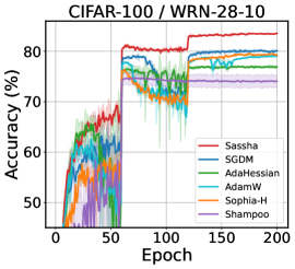
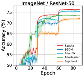
We first evaluate Sassha for image classification on CIFAR-10, CIFAR-100, and ImageNet. We train various models of the ResNet family (He et al., 2016; Zagoruyko & Komodakis, 2016) and an efficient variant of Vision Transformer (Beyer et al., 2022). We adhere to standard inception-style data augmentations during training instead of making use of advanced data augmentation techniques (DeVries & Taylor, 2017) or regularization methods (Gastaldi, 2017). Results are presented in Table˜2 and Figure˜3.

We begin by comparing the generalization performance of adaptive second-order methods to that of first-order methods. Across all settings, adaptive second-order methods consistently exhibit lower accuracy than their first-order counterparts. This observation aligns with previous studies indicating that second-order optimization often result in poorer generalization compared to first-order approaches. In contrast, Sassha, benefiting from sharpness minimization, consistently demonstrates superior generalization performance, outperforming both first-order and second-order methods in every setting. Particularly, Sassha is up to 4% more effective than the best-performing adaptive or second-order methods (e.g., WRN-28-10, ViT-s-32). Moreover, Sassha continually surpasses SGD and AdamW, even when they are trained for twice as many epochs, achieving a performance margin of about 0.3% to 3%. Further details are provided in Appendix˜G.

Interestingly, Sassha also outperforms SAM. Since first-order methods typically exhibit superior generalization performance compared to second-order methods, it might be intuitive to expect SAM to surpass Sassha if the two are viewed merely as the outcomes of applying sharpness minimization to first-order and second-order methods, respectively. However, the results conflict with this intuition. We attribute this to the careful design choices made in Sassha, stabilizing Hessian approximation under sharpness minimization, so as to unleash the potential of the second-order method, leading to its outstanding performance. As a support, we show that naively incorporating SAM into other second-order methods does not yield these favorable results in Appendix˜H. We also make more comparisons with SAM in Section˜5.3.

5.2 Language Modeling

Recent studies have shown the potential of second-order methods for pretraining language models. Here, we first evaluate how Sassha performs on this task. Specifically, we train GPT1-mini, a scaled-down variant of GPT1 (Radford et al., 2019), on Wikitext-2 dataset (Merity et al., 2022) using various methods including Sassha and compare their results (see the left of Table˜3). Our results show that Sassha achieves the lowest perplexity among all methods including Sophia-H (Liu et al., 2024), a recent method that is designed specifically for language modeling tasks and sets state of the art, which highlights generality in addition to the numerical advantage of Sassha.

We also extend our evaluation to finetuning tasks. Specifically, we finetune SqueezeBERT (Iandola et al., 2020) for diverse tasks in the GLUE benchmark (Wang et al., 2018). The results are on the right side of Table˜3. It shows that Sassha compares competitively to other second-order methods. Notably, it also outperforms AdamW—often the method of choice for training language models—on nearly all tasks.

5.3 Comparison to SAM

So far, we have seen that Sassha outperforms second-order methods quite consistently on both vision and language tasks. Interestingly, we also find that Sassha often improves upon SAM. In particular, it appears that the gain is larger for the Transformer-based architectures, i.e., ViT results in Table˜2 or GPT/BERT results in Table˜3.

We posit that this is potentially due to the robustness of Sassha to the block heterogeneity inherent in Transformer architectures, where the Hessian spectrum varies significantly across different blocks. This characteristic is known to make SGD perform worse than adaptive methods like Adam on Transformer-based models (Zhang et al., 2024). Since Sassha leverages second-order information via preconditioning gradients, it has the potential to address the ill-conditioned nature of Transformers more effectively than SAM with first-order methods.

To push further, we conducted additional experiments. First, we allocate more training budgets to SAM to see whether it compares to Sassha. The results are presented in Table˜4. We find that SAM still underperforms Sassha, even though it is given more budgets of training iterations over data or wall-clock time. Furthermore, we also compare Sassha to more advanced variants of SAM including ASAM (Kwon et al., 2021) and GSAM (Zhuang et al., 2022), showing that Sassha performs competitively even to these methods (Appendix˜I). Notably, however, these variants of SAM require a lot more hyperparameter tuning to be compared.

6 Further Analysis

Table 4: Comparison between Sassha and SAM with more training budgets for the ViT-s-32 / ImageNet workload.
Epoch Time (s) Accuracy (%)
SAM ${}_{\text{ SGD}}$ 180 220,852 65.403±0.6365.403_{{\color[rgb]{0.4,0.4,0.4}\definecolor[named]{pgfstrokecolor}{rgb}{0.4,0.4,0.4}\pgfsys@color@gray@stroke{0.4}\pgfsys@color@gray@fill{0.4}\pm 0.63}}
SAM ${}_{\text{ AdamW}}$ 180 234,374 68.706±0.1668.706_{{\color[rgb]{0.4,0.4,0.4}\definecolor[named]{pgfstrokecolor}{rgb}{0.4,0.4,0.4}\pgfsys@color@gray@stroke{0.4}\pgfsys@color@gray@fill{0.4}\pm 0.16}}
Sassha 90 123,948 69.195±0.30\textbf{69.195}_{{\color[rgb]{0.4,0.4,0.4}\definecolor[named]{pgfstrokecolor}{rgb}{0.4,0.4,0.4}\pgfsys@color@gray@stroke{0.4}\pgfsys@color@gray@fill{0.4}\pm 0.30}}

6.1 Robustness

Noisily labeled training data can critically degrade generalization performance (Natarajan et al., 2013). To evaluate how Sassha generalizes under these practical conditions, we randomly corrupt certain fractions of the training data and compare the validation performances between different methods. The results show that Sassha outperforms other methods across all noise levels with minimal accuracy degradation (Table˜5). Additionally, we also observe the same trend on CIFAR-10 (Table˜20).

Interestingly, Sassha surpasses SAM (Foret et al., 2021), which is known to be one of the most robust techniques against label noise (Baek et al., 2024). We hypothesize that its robustness stems from the complementary benefits of the sharpness-minimization scheme and second-order methods. Specifically, SAM enhances robustness by adversarially perturbing the parameters and giving more importance to clean data during optimization, making the model more resistant to label noise (Foret et al., 2021; Baek et al., 2024). Also, recent research indicates that second-order methods are robust to label noise due to preconditioning that reduces the variance in the population risk (Amari et al., 2021).

Table 5: Validation accuracy measured for ResNet-32/CIFAR-100 at different levels of noise. Sassha shows the best robustness.
Noise level
Method 0% 20% 40% 60%
SGD 69.32±0.1969.32_{{\color[rgb]{0.4,0.4,0.4}\definecolor[named]{pgfstrokecolor}{rgb}{0.4,0.4,0.4}\pgfsys@color@gray@stroke{0.4}\pgfsys@color@gray@fill{0.4}\pm 0.19}} 62.18±0.0662.18_{{\color[rgb]{0.4,0.4,0.4}\definecolor[named]{pgfstrokecolor}{rgb}{0.4,0.4,0.4}\pgfsys@color@gray@stroke{0.4}\pgfsys@color@gray@fill{0.4}\pm 0.06}} 55.78±0.5555.78_{{\color[rgb]{0.4,0.4,0.4}\definecolor[named]{pgfstrokecolor}{rgb}{0.4,0.4,0.4}\pgfsys@color@gray@stroke{0.4}\pgfsys@color@gray@fill{0.4}\pm 0.55}} 45.53±0.7845.53_{{\color[rgb]{0.4,0.4,0.4}\definecolor[named]{pgfstrokecolor}{rgb}{0.4,0.4,0.4}\pgfsys@color@gray@stroke{0.4}\pgfsys@color@gray@fill{0.4}\pm 0.78}}
SAM ${}_{\text{SGD}}$ 71.99±0.2071.99_{{\color[rgb]{0.4,0.4,0.4}\definecolor[named]{pgfstrokecolor}{rgb}{0.4,0.4,0.4}\pgfsys@color@gray@stroke{0.4}\pgfsys@color@gray@fill{0.4}\pm 0.20}} 65.53±0.1165.53_{{\color[rgb]{0.4,0.4,0.4}\definecolor[named]{pgfstrokecolor}{rgb}{0.4,0.4,0.4}\pgfsys@color@gray@stroke{0.4}\pgfsys@color@gray@fill{0.4}\pm 0.11}} 61.20±0.1761.20_{{\color[rgb]{0.4,0.4,0.4}\definecolor[named]{pgfstrokecolor}{rgb}{0.4,0.4,0.4}\pgfsys@color@gray@stroke{0.4}\pgfsys@color@gray@fill{0.4}\pm 0.17}} 51.93±0.4751.93_{{\color[rgb]{0.4,0.4,0.4}\definecolor[named]{pgfstrokecolor}{rgb}{0.4,0.4,0.4}\pgfsys@color@gray@stroke{0.4}\pgfsys@color@gray@fill{0.4}\pm 0.47}}
AdaHessian 68.06±0.2268.06_{{\color[rgb]{0.4,0.4,0.4}\definecolor[named]{pgfstrokecolor}{rgb}{0.4,0.4,0.4}\pgfsys@color@gray@stroke{0.4}\pgfsys@color@gray@fill{0.4}\pm 0.22}} 63.06±0.2563.06_{{\color[rgb]{0.4,0.4,0.4}\definecolor[named]{pgfstrokecolor}{rgb}{0.4,0.4,0.4}\pgfsys@color@gray@stroke{0.4}\pgfsys@color@gray@fill{0.4}\pm 0.25}} 58.37±0.1358.37_{{\color[rgb]{0.4,0.4,0.4}\definecolor[named]{pgfstrokecolor}{rgb}{0.4,0.4,0.4}\pgfsys@color@gray@stroke{0.4}\pgfsys@color@gray@fill{0.4}\pm 0.13}} 46.02±1.9646.02_{{\color[rgb]{0.4,0.4,0.4}\definecolor[named]{pgfstrokecolor}{rgb}{0.4,0.4,0.4}\pgfsys@color@gray@stroke{0.4}\pgfsys@color@gray@fill{0.4}\pm 1.96}}
Sophia-H 67.76±0.3767.76_{{\color[rgb]{0.4,0.4,0.4}\definecolor[named]{pgfstrokecolor}{rgb}{0.4,0.4,0.4}\pgfsys@color@gray@stroke{0.4}\pgfsys@color@gray@fill{0.4}\pm 0.37}} 62.34±0.4762.34_{{\color[rgb]{0.4,0.4,0.4}\definecolor[named]{pgfstrokecolor}{rgb}{0.4,0.4,0.4}\pgfsys@color@gray@stroke{0.4}\pgfsys@color@gray@fill{0.4}\pm 0.47}} 56.54±0.2856.54_{{\color[rgb]{0.4,0.4,0.4}\definecolor[named]{pgfstrokecolor}{rgb}{0.4,0.4,0.4}\pgfsys@color@gray@stroke{0.4}\pgfsys@color@gray@fill{0.4}\pm 0.28}} 45.37±0.2745.37_{{\color[rgb]{0.4,0.4,0.4}\definecolor[named]{pgfstrokecolor}{rgb}{0.4,0.4,0.4}\pgfsys@color@gray@stroke{0.4}\pgfsys@color@gray@fill{0.4}\pm 0.27}}
Shampoo 64.08±0.4664.08_{{\color[rgb]{0.4,0.4,0.4}\definecolor[named]{pgfstrokecolor}{rgb}{0.4,0.4,0.4}\pgfsys@color@gray@stroke{0.4}\pgfsys@color@gray@fill{0.4}\pm 0.46}} 58.85±0.6658.85_{{\color[rgb]{0.4,0.4,0.4}\definecolor[named]{pgfstrokecolor}{rgb}{0.4,0.4,0.4}\pgfsys@color@gray@stroke{0.4}\pgfsys@color@gray@fill{0.4}\pm 0.66}} 53.82±0.7153.82_{{\color[rgb]{0.4,0.4,0.4}\definecolor[named]{pgfstrokecolor}{rgb}{0.4,0.4,0.4}\pgfsys@color@gray@stroke{0.4}\pgfsys@color@gray@fill{0.4}\pm 0.71}} 42.91±0.9942.91_{{\color[rgb]{0.4,0.4,0.4}\definecolor[named]{pgfstrokecolor}{rgb}{0.4,0.4,0.4}\pgfsys@color@gray@stroke{0.4}\pgfsys@color@gray@fill{0.4}\pm 0.99}}
Sassha 72.14±0.16\textbf{72.14}_{{\color[rgb]{0.4,0.4,0.4}\definecolor[named]{pgfstrokecolor}{rgb}{0.4,0.4,0.4}\pgfsys@color@gray@stroke{0.4}\pgfsys@color@gray@fill{0.4}\pm 0.16}} 66.78±0.47\textbf{66.78}_{{\color[rgb]{0.4,0.4,0.4}\definecolor[named]{pgfstrokecolor}{rgb}{0.4,0.4,0.4}\pgfsys@color@gray@stroke{0.4}\pgfsys@color@gray@fill{0.4}\pm 0.47}} 61.97±0.27\textbf{ 61.97}_{{\color[rgb]{0.4,0.4,0.4}\definecolor[named]{pgfstrokecolor}{rgb}{0.4,0.4,0.4}\pgfsys@color@gray@stroke{0.4}\pgfsys@color@gray@fill{0.4}\pm 0.27}} 53.98±0.57\textbf{ 53.98}_{{\color[rgb]{0.4,0.4,0.4}\definecolor[named]{pgfstrokecolor}{rgb}{0.4,0.4,0.4}\pgfsys@color@gray@stroke{0.4}\pgfsys@color@gray@fill{0.4}\pm 0.57}}
Refer to caption
(a) Train loss
Refer to caption
(b) Update size
Refer to caption
(c) $D$ distribution
Figure 4: Effects of square-root measured for ResNet-32/CIFAR-100; $D$ is set to be either $|\widehat{H}|^{1/2}$ for Sassha or $|\widehat{H}|$ for No-Sqrt. Sharpness minimization drives the diagonal Hessian entries move towards zero, causing divergence. The square-root in Sassha helps counteract this effect, stabilizing the training process.

6.2 Stability

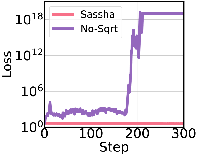
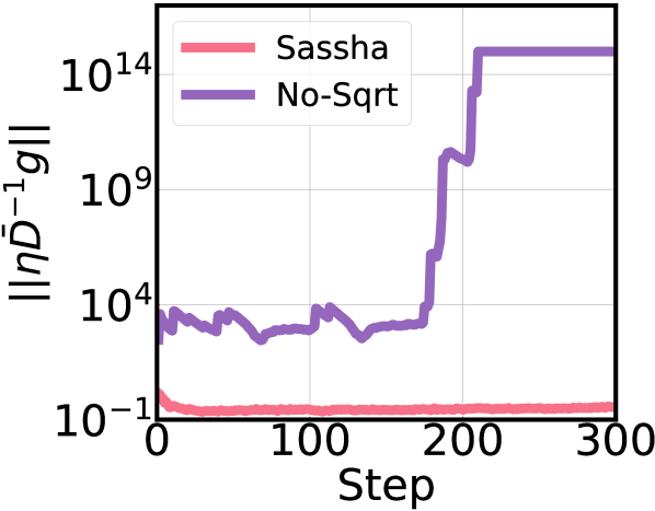
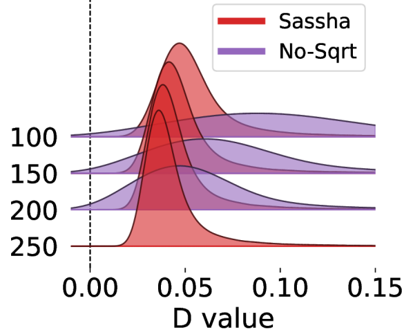
To show the effect of the square-root function on stabilizing the training process, we run Sassha without the square-root (No-Sqrt), repeatedly for multiple times with different random seeds. As a result, we find that the training diverges most of the time. A failure case is depicted in Figure˜4.

At first, we find that the level of training loss for No-Sqrt is much higher than that of Sassha, and also, it spikes up around step $200$ (Figure˜4(a)). To look into it further, we also measure the update sizes along the trajectory (Figure˜4(b)). The results show that it matches well with the loss curves, suggesting that the training failure is somehow due to taking too large steps.

It turns out that this problem stems from the preconditioning matrix $D$ being too small; i.e., the distribution of diagonal entries in the preconditioning matrix gradually shifts toward zero values (Figure˜4(c)); as a result, $D^{-1}$ becomes too large, creating large steps. This progressive increase in near-zero diagonal Hessian entries is precisely due to the sharpness minimization scheme that we introduced; it penalizes the Hessian eigenspectrum to yield flat solutions, yet it could also make training unstable if taken naively. By including square-root, the preconditioner are less situated near zero, effectively suppressing the risk of large updates, thereby stabilizing the training process. We validate this further by showing its superiority to other alternatives including damping and clipping in Section˜E.1.

We also provide an ablation analysis for the absolute-value function in Section˜E.2, which demonstrates that it increases the stability of Sassha in tandem with square-root.

Refer to caption
Refer to caption
(a) Lazy Hessian
Refer to caption
(b) $\widehat{H}$ change
Refer to caption
(c) Local sensitivity
Figure 5: Effect of lazy Hessian for ResNet-32/CIFAR-100. Sassha stays within the region where the Hessian varies small.

6.3 Efficiency

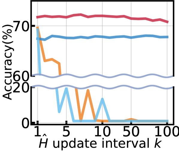
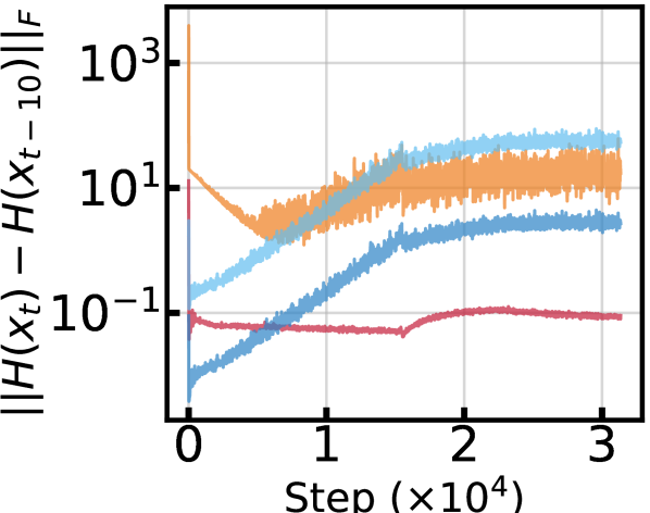
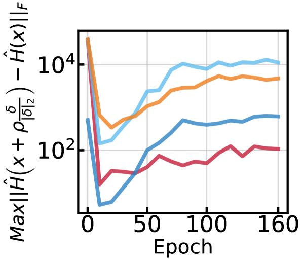
Here we show the effectiveness of lazy Hessian updates in Sassha. The results are shown in Figure˜5. At first, we see that Sassha maintains its performance even at $k=100$, indicating that it is extremely robust to lazy Hessian updates (Figure˜5(a)). We also measure the difference between the current and previous Hessians to validate lazy Hessian updates more directly (Figure˜5(b)). The result shows that Sassha keeps the changes in Hessian to be small, and much smaller than other methods, indicating its advantage of robust reuse, and hence, computational efficiency.

We attribute this robustness to the sharpness minimization scheme incorporated in Sassha, which can potentially bias optimization toward the region of low curvature sensitivity. To verify, we define local Hessian sensitivity as follows:

$$\max_{\delta\sim\mathcal{N}(0,1)}\left\|\widehat{H}\left(x+\rho\frac{\delta}{\|\delta\|_{2}}\right)-\widehat{H}(x)\right\|_{F}$$ (4)

i.e., it measures the maximum change in Hessian induced from normalized random perturbations. A smaller Hessian sensitivity would suggest reduced variability in the loss curvature, leading to greater relevance of the current Hessian for subsequent optimization steps. We find that Sassha is far less sensitive compared to other methods (Figure˜5(c)).

6.4 Cost

Second-order methods can be highly costly. In this section, we discuss the computational cost of Sassha and reveal its competitiveness to other methods.

Sassha requires one gradient computation (GC) in the sharpness minimization step, one Hessian-vector product (HVP) for diagonal Hessian computation, and an additional GC in the descent step. That is, a total of $2$GCs and $1$HVP are required. However, with lazy Hessian updates, the number of HVPs reduces drastically to $1/k$. With $k=10$ as the default value used in this work, this scales down to $0.1$HVPs.

It turns out that this is critical to the utility of Sassha, because $1$HVP is known to take about $\times 3$ the computation time of $1$GC in practice (Dagréou et al., 2024). Compared to conventional second-order methods ($1$GC $+$ $1$HVP $\simeq$ $4$GCs), the cost of Sassha can roughly be a half of that ($2.3$GCs). It is also comparable to standard SAM variants ($2$GCs).

Furthermore, we can leverage a momentum of gradients in the perturbation step to reduce the cost. This variant M-Sassha requires only $1.3$GCs with minimal decrease in performance. Notably, M-Sassha still outperforms standard first-order methods like SGD and AdamW (Appendix˜K).

To verify, we measure the average wall-clock times and present the results in Table˜6. First, one can see that the theoretical cost is reflected well on the actual cost; i.e., the time measurements scales proportionally roughly well with respect to the total cost. More importantly, this result indicates the potential of Sassha for performance-critical applications. Considering its well-balanced cost, and that it has been challenging to employ second-order methods efficiently for large-scale tasks without sacrificing performance, Sassha can be a reasonable addition to the lineup.

Table 6: Average wall-clock time per epoch (s) and the theoretical cost of different methods. Sassha can be an effective alternative to existing methods for its enhanced generalization performance.
Method Cost CIFAR10 CIFAR100 ImageNet
Descent Sharpness Hessian Total ResNet32 WRN28-10 ViT-small
AdamW 1 GC 0 GC 0 HVP 1 GC 5.03 59.29 976.56
SAM 1 GC 1 GC 0 HVP 2 GC 9.16 118.46 1302.08
AdaHessian 1 GC 0 GC 1 HVP 4 GC 33.75 296.63 2489.07
Sassha 1 GC 1 GC 0.1 HVP 2.3 GC 12.00 142.06 1377.20
M-Sassha 1 GC 0 GC 0.1 HVP 1.3 GC 8.91 84.12 1065.40

7 Conclusion

In this work, we focus on addressing the issue of poor generalization in approximate second-order methods. To this end, we propose a new method called Sassha that stably minimizes sharpness within the framework of second-order optimization. Sassha converges to flat solutions and achieves state-of-the-art performance within this class. Sassha also performs competitively to widely-used first-order, adaptive, and sharpness-aware methods. Sassha achieves this in robust, stable, and efficient ways without incurring much cost or requiring extra hyperparameter tuning. All of these are rigorously assessed with extensive experiments.

Nonetheless, there are many limitations to be addressed in this work for more improvements which may include, but are not limited to, extending experiments to extreme scales of various models and different data, and consolidating theoretical foundations. Seeing it as an exciting opportunity, we plan to investigate further in future work.

8 Acknowledgement

This work was partly supported by the Institute of Information & communications Technology Planning & Evaluation (IITP) grant funded by the Korean government (MSIT) (IITP-2019-0-01906, Artificial Intelligence Graduate School Program (POSTECH), RS-2022-II220959, (part2) Few-Shot learning of Causal Inference in Vision and Language for Decision Making, and RS-2024-00338140, Development of learning and utilization technology to reflect sustainability of generative language models and up-to-dateness over time), and the National Research Foundation of Korea (NRF) grant funded by the Korean government (MSIT) ( NRF-2022R1F1A1064569, RS-2023-00210466, RS-2023-00265444).

References

  • Agarwala & Dauphin (2023) Agarwala, A. and Dauphin, Y. Sam operates far from home: eigenvalue regularization as a dynamical phenomenon. ICML, 2023.
  • Amari et al. (2000) Amari, S.-i., Park, H., and Fukumizu, K. Adaptive method of realizing natural gradient learning for multilayer perceptrons. Neural computation, 2000.
  • Amari et al. (2021) Amari, S.-i., Ba, J., Grosse, R. B., Li, X., Nitanda, A., Suzuki, T., Wu, D., and Xu, J. When does preconditioning help or hurt generalization? ICLR, 2021.
  • Baek et al. (2024) Baek, C., Kolter, J. Z., and Raghunathan, A. Why is SAM robust to label noise? ICLR, 2024.
  • Bahri et al. (2022) Bahri, D., Mobahi, H., and Tay, Y. Sharpness-aware minimization improves language model generalization. ACL, 2022.
  • Becker et al. (2024) Becker, M., Altrock, F., and Risse, B. Momentum-sam: Sharpness aware minimization without computational overhead. arXiv, 2024.
  • Becker et al. (1988) Becker, S., Le Cun, Y., et al. Improving the convergence of back-propagation learning with second order methods. CMSS, 1988.
  • Beyer et al. (2022) Beyer, L., Zhai, X., and Kolesnikov, A. Better plain vit baselines for imagenet-1k. arXiv preprint arXiv:2205.01580, 2022.
  • Botev et al. (2017) Botev, A., Ritter, H., and Barber, D. Practical gauss-newton optimisation for deep learning. ICML, 2017.
  • Bottou et al. (2018) Bottou, L., Curtis, F. E., and Nocedal, J. Optimization methods for large-scale machine learning. SIAM Review, 60(2):223–311, 2018.
  • Byrd et al. (2016) Byrd, R. H., Hansen, S. L., Nocedal, J., and Singer, Y. A stochastic quasi-newton method for large-scale optimization. SIAM Journal on Optimization, 2016.
  • Chaudhari et al. (2017) Chaudhari, P., Choromanska, A., Soatto, S., LeCun, Y., Baldassi, C., Borgs, C., Chayes, J., Sagun, L., and Zecchina, R. Entropy-SGD: Biasing gradient descent into wide valleys. ICLR, 2017.
  • Chen et al. (2022) Chen, X., Hsieh, C.-J., and Gong, B. When vision transformers outperform resnets without pre-training or strong data augmentations. ICLR, 2022.
  • Dagréou et al. (2024) Dagréou, M., Ablin, P., Vaiter, S., and Moreau, T. How to compute hessian-vector products? The Third Blogpost Track at ICLR, 2024.
  • Dauphin et al. (2015) Dauphin, Y., De Vries, H., and Bengio, Y. Equilibrated adaptive learning rates for non-convex optimization. NeurIPS, 2015.
  • Dauphin et al. (2014) Dauphin, Y. N., Pascanu, R., Gulcehre, C., Cho, K., Ganguli, S., and Bengio, Y. Identifying and attacking the saddle point problem in high-dimensional non-convex optimization. NeurIPS, 2014.
  • Demeniconi & Chawla (2020) Demeniconi, C. and Chawla, N. Second-order optimization for non-convex machine learning: an empirical study. Society for Industrial and Applied Mathematics, 2020.
  • DeVries & Taylor (2017) DeVries, T. and Taylor, G. W. Improved regularization of convolutional neural networks with cutout. arXiv preprint arXiv:1708.04552, 2017.
  • Dinh et al. (2017) Dinh, L., Pascanu, R., Bengio, S., and Bengio, Y. Sharp minima can generalize for deep nets. ICML, 2017.
  • Doikov et al. (2023) Doikov, N., Chayti, E. M., and Jaggi, M. Second-order optimization with lazy hessians. ICML, 2023.
  • Du et al. (2022a) Du, J., Yan, H., Feng, J., Zhou, J. T., Zhen, L., Goh, R. S. M., and Tan, V. Efficient sharpness-aware minimization for improved training of neural networks. ICLR, 2022a.
  • Du et al. (2022b) Du, J., Zhou, D., Feng, J., Tan, V., and Zhou, J. T. Sharpness-aware training for free. NeurIPS, 2022b.
  • Duchi et al. (2011) Duchi, J., Hazan, E., and Singer, Y. Adaptive subgradient methods for online learning and stochastic optimization. JMLR, 2011.
  • Dziugaite & Roy (2017) Dziugaite, G. K. and Roy, D. M. Computing nonvacuous generalization bounds for deep (stochastic) neural networks with many more parameters than training data. In Proceedings of the 33rd Annual Conference on Uncertainty in Artificial Intelligence (UAI), 2017.
  • Foret et al. (2021) Foret, P., Kleiner, A., Mobahi, H., and Neyshabur, B. Sharpness-aware minimization for efficiently improving generalization. ICLR, 2021.
  • Gastaldi (2017) Gastaldi, X. Shake-shake regularization. arXiv preprint arXiv:1705.07485, 2017.
  • Goldfarb et al. (2020) Goldfarb, D., Ren, Y., and Bahamou, A. Practical quasi-newton methods for training deep neural networks. NeurIPS, 2020.
  • Gomes et al. (2024) Gomes, D. M., Zhang, Y., Belilovsky, E., Wolf, G., and Hosseini, M. S. Adafisher: Adaptive second order optimization via fisher information. arXiv preprint arXiv:2405.16397, 2024.
  • Gower et al. (2016) Gower, R., Goldfarb, D., and Richtárik, P. Stochastic block bfgs: Squeezing more curvature out of data. ICML, 2016.
  • Gupta et al. (2018) Gupta, V., Koren, T., and Singer, Y. Shampoo: Preconditioned stochastic tensor optimization. In ICLR, 2018.
  • Hardt et al. (2016) Hardt, M., Recht, B., and Singer, Y. Train faster, generalize better: Stability of stochastic gradient descent. ICML, 2016.
  • He et al. (2016) He, K., Zhang, X., Ren, S., and Sun, J. Deep residual learning for image recognition. CVPR, 2016.
  • Hinton et al. (2012) Hinton, G., Srivastava, N., and Swersky, K. Neural networks for machine learning lecture 6a overview of mini-batch gradient descent. Coursera Lecture slides https://class. coursera. org/neuralnets-2012-001/lecture, 2012.
  • Hochreiter & Schmidhuber (1994) Hochreiter, S. and Schmidhuber, J. Simplifying neural nets by discovering flat minima. NeurIPS, 1994.
  • Hochreiter & Schmidhuber (1997) Hochreiter, S. and Schmidhuber, J. Flat minima. Neural Computation, 1997.
  • Hutchinson (1989) Hutchinson, M. A stochastic estimator of the trace of the influence matrix for laplacian smoothing splines. Communications in Statistics - Simulation and Computation, 18(3):1059–1076, 1989.
  • Iandola et al. (2020) Iandola, F., Shaw, A., Krishna, R., and Keutzer, K. Squeezebert: What can computer vision teach nlp about efficient neural networks? SustaiNLP: Workshop on Simple and Efficient Natural Language Processing, 2020.
  • Izmailov et al. (2018) Izmailov, P., Podoprikhin, D., Garipov, T., Vetrov, D., and Wilson, A. G. Averaging weights leads to wider optima and better generalization. UAI, 2018.
  • Jastrzębski et al. (2018) Jastrzębski, S., Kenton, Z., Ballas, N., Fischer, A., Bengio, Y., and Storkey, A. On the relation between the sharpest directions of dnn loss and the sgd step length. ICLR, 2018.
  • Jiang et al. (2020) Jiang, Y., Neyshabur, B., Mobahi, H., Krishnan, D., and Bengio, S. Fantastic generalization measures and where to find them. ICLR, 2020.
  • Karimireddy et al. (2019) Karimireddy, S. P., Rebjock, Q., Stich, S., and Jaggi, M. Error feedback fixes signsgd and other gradient compression schemes. ICML, 2019.
  • Keskar et al. (2017) Keskar, N. S., Mudigere, D., Nocedal, J., Smelyanskiy, M., and Tang, P. T. P. On large-batch training for deep learning: Generalization gap and sharp minima. ICLR, 2017.
  • Khanh et al. (2024) Khanh, P. D., Luong, H.-C., Mordukhovich, B. S., and Tran, D. B. Fundamental convergence analysis of sharpness-aware minimization. NeurIPS, 2024.
  • Kingma & Ba (2015) Kingma, D. P. and Ba, J. Adam: A method for stochastic optimization. ICLR, 2015.
  • Kiros (2013) Kiros, R. Training neural networks with stochastic hessian-free optimization. arXiv preprint arXiv:1301.3641, 2013.
  • Kunstner et al. (2019) Kunstner, F., Hennig, P., and Balles, L. Limitations of the empirical fisher approximation for natural gradient descent. NeurIPS, 32, 2019.
  • Kwon et al. (2021) Kwon, J., Kim, J., Park, H., and Choi, I. K. Asam: Adaptive sharpness-aware minimization for scale-invariant learning of deep neural networks. ICML, 2021.
  • Li et al. (2023) Li, H., Rakhlin, A., and Jadbabaie, A. Convergence of adam under relaxed assumptions. NeurIPS, 2023.
  • Liu et al. (2024) Liu, H., Li, Z., Hall, D., Liang, P., and Ma, T. Sophia: A scalable stochastic second-order optimizer for language model pre-training. ICLR, 2024.
  • Liu et al. (2022) Liu, Y., Mai, S., Chen, X., Hsieh, C.-J., and You, Y. Towards efficient and scalable sharpness-aware minimization. CVPR, 2022.
  • Loshchilov & Hutter (2018) Loshchilov, I. and Hutter, F. Decoupled weight decay regularization. ICLR, 2018.
  • Martens & Grosse (2015) Martens, J. and Grosse, R. Optimizing neural networks with kronecker-factored approximate curvature. ICML, 2015.
  • Martens et al. (2010) Martens, J. et al. Deep learning via hessian-free optimization. ICML, 2010.
  • Merity et al. (2022) Merity, S., Xiong, C., Bradbury, J., and Socher, R. Pointer sentinel mixture models. ICLR, 2022.
  • Mi et al. (2022) Mi, P., Shen, L., Ren, T., Zhou, Y., Sun, X., Ji, R., and Tao, D. Make sharpness-aware minimization stronger: A sparsified perturbation approach. NeurIPS, 2022.
  • Murray (2010) Murray, W. Newton-type methods. Wiley Encyclopedia of Operations Research and Management Science, 2010.
  • Natarajan et al. (2013) Natarajan, N., Dhillon, I. S., Ravikumar, P. K., and Tewari, A. Learning with noisy labels. NeurIPS, 2013.
  • Neyshabur et al. (2017) Neyshabur, B., Bhojanapalli, S., Mcallester, D., and Srebro, N. Exploring generalization in deep learning. NeurIPS, 2017.
  • Nocedal & Wright (1999) Nocedal, J. and Wright, S. J. Numerical optimization. Springer, 1999.
  • Orvieto et al. (2022) Orvieto, A., Kersting, H., Proske, F., Bach, F., and Lucchi, A. Anticorrelated noise injection for improved generalization. ICML, 2022.
  • Qu et al. (2022) Qu, Z., Li, X., Duan, R., Liu, Y., Tang, B., and Lu, Z. Generalized federated learning via sharpness aware minimization. ICML, 2022.
  • Radford et al. (2019) Radford, A., Wu, J., Child, R., Luan, D., Amodei, D., Sutskever, I., et al. Language models are unsupervised multitask learners. OpenAI blog, 2019.
  • Roosta-Khorasani & Ascher (2014) Roosta-Khorasani, F. and Ascher, U. Improved bounds on sample size for implicit matrix trace estimators. FoCM, 2014.
  • Schraudolph (2002) Schraudolph, N. N. Fast curvature matrix-vector products for second-order gradient descent. Neural computation, 2002.
  • Shin et al. (2024) Shin, S., Lee, D., Andriushchenko, M., and Lee, N. Critical influence of overparameterization on sharpness-aware minimization. arXiv, 2024.
  • Wadia et al. (2021) Wadia, N., Duckworth, D., Schoenholz, S. S., Dyer, E., and Sohl-Dickstein, J. Whitening and second order optimization both make information in the dataset unusable during training, and can reduce or prevent generalization. ICML, 2021.
  • Wang et al. (2018) Wang, A., Singh, A., Michael, J., Hill, F., Levy, O., and Bowman, S. R. Glue: A multi-task benchmark and analysis platform for natural language understanding. ICLR, 2018.
  • Wang et al. (2013) Wang, W. J., Zhu, J. B., and Duan, X. J. Eigenvalue decomposition based modified newton algorithm. AMM, 2013.
  • Wilson et al. (2017) Wilson, A. C., Roelofs, R., Stern, M., Srebro, N., and Recht, B. The marginal value of adaptive gradient methods in machine learning. NeurIPS, 2017.
  • Wolf et al. (2020) Wolf, T., Debut, L., Sanh, V., Chaumond, J., Delangue, C., Moi, A., Cistac, P., Rault, T., Louf, R., Funtowicz, M., Davison, J., Shleifer, S., von Platen, P., Ma, C., Jernite, Y., Plu, J., Xu, C., Scao, T. L., Gugger, S., Drame, M., Lhoest, Q., and Rush, A. M. Huggingface’s transformers: State-of-the-art natural language processing. arXiv, 2020.
  • Xie et al. (2020) Xie, Z., Sato, I., and Sugiyama, M. A diffusion theory for deep learning dynamics: Stochastic gradient descent exponentially favors flat minima. ICLR, 2020.
  • Yao et al. (2020) Yao, Z., Gholami, A., Keutzer, K., and Mahoney, M. W. Pyhessian: Neural networks through the lens of the hessian. IEEE BigData, 2020.
  • Yao et al. (2021) Yao, Z., Gholami, A., Shen, S., Keutzer, K., and Mahoney, M. W. Adahessian: An adaptive second order optimizer for machine learning. AAAI, 2021.
  • Zagoruyko & Komodakis (2016) Zagoruyko, S. and Komodakis, N. Wide residual networks. BMVC, 2016.
  • Zhang et al. (2024) Zhang, Y., Chen, C., Ding, T., Li, Z., Sun, R., and Luo, Z.-Q. Why transformers need adam: A hessian perspective. NeurIPS, 2024.
  • Zhou et al. (2020) Zhou, P., Feng, J., Ma, C., Xiong, C., Hoi, S. C. H., et al. Towards theoretically understanding why sgd generalizes better than adam in deep learning. NeurIPS, 2020.
  • Zhuang et al. (2022) Zhuang, J., Gong, B., Yuan, L., Cui, Y., Adam, H., Dvornek, N. C., sekhar tatikonda, s Duncan, J., and Liu, T. Surrogate gap minimization improves sharpness-aware training. ICLR, 2022.
  • Zou et al. (2022) Zou, D., Cao, Y., Li, Y., and Gu, Q. Understanding the generalization of adam in learning neural networks with proper regularization. ICLR, 2022.

Appendix A Sharpness Measurements for Other Settings

Table 7: Sharpness measurements of the solutions found by seven different optimizers and their generalization on CIFAR-10/100 and Wikitext-2. Approximate second-order methods tend to yield highly sharp solutions and poor generalization compared to SGD; Sassha and M-Sassha effectively recover this. Here, we measure sharpness in terms of maximum Hessian eigenvalue $\lambda_{max}(H)$, trace of Hessian $\operatorname{tr}(H)$, worst-case sharpness $\delta L_{\text{worst}}$, and average sharpness $\delta L_{\text{avg}}$, along with generalization using validation loss $L_{val}$ and accuracy $\text{Acc}_{val}$.
Sharpness Generalization
$\lambda_{max}(H)$ $\operatorname{tr}(H)_{\times 10^{3}}$ $\delta L_{\text{worst}}$ $\delta L_{\text{avg}\times 10^{-3}}$ $L_{\text{val}}$ $\text{Acc}_{\text{val}}$
CIFAR-10
ResNet20 SGD 107±4.37107_{{\color[rgb]{0.4,0.4,0.4}\definecolor[named]{pgfstrokecolor}{rgb}{0.4,0.4,0.4}\pgfsys@color@gray@stroke{0.4}\pgfsys@color@gray@fill{0.4}\pm 4.37}} 1.38±0.011.38_{{\color[rgb]{0.4,0.4,0.4}\definecolor[named]{pgfstrokecolor}{rgb}{0.4,0.4,0.4}\pgfsys@color@gray@stroke{0.4}\pgfsys@color@gray@fill{0.4}\pm 0.01}} 0.840±0.3040.840_{{\color[rgb]{0.4,0.4,0.4}\definecolor[named]{pgfstrokecolor}{rgb}{0.4,0.4,0.4}\pgfsys@color@gray@stroke{0.4}\pgfsys@color@gray@fill{0.4}\pm 0.304}} 0.690±0.390.690_{{\color[rgb]{0.4,0.4,0.4}\definecolor[named]{pgfstrokecolor}{rgb}{0.4,0.4,0.4}\pgfsys@color@gray@stroke{0.4}\pgfsys@color@gray@fill{0.4}\pm 0.39}} 0.295±0.0080.295_{{\color[rgb]{0.4,0.4,0.4}\definecolor[named]{pgfstrokecolor}{rgb}{0.4,0.4,0.4}\pgfsys@color@gray@stroke{0.4}\pgfsys@color@gray@fill{0.4}\pm 0.008}} 92.03±0.3292.03_{{\color[rgb]{0.4,0.4,0.4}\definecolor[named]{pgfstrokecolor}{rgb}{0.4,0.4,0.4}\pgfsys@color@gray@stroke{0.4}\pgfsys@color@gray@fill{0.4}\pm 0.32}}
SAM 58±2.9858_{{\color[rgb]{0.4,0.4,0.4}\definecolor[named]{pgfstrokecolor}{rgb}{0.4,0.4,0.4}\pgfsys@color@gray@stroke{0.4}\pgfsys@color@gray@fill{0.4}\pm 2.98}} 0.73±0.040.73_{{\color[rgb]{0.4,0.4,0.4}\definecolor[named]{pgfstrokecolor}{rgb}{0.4,0.4,0.4}\pgfsys@color@gray@stroke{0.4}\pgfsys@color@gray@fill{0.4}\pm 0.04}} 0.171±0.0380.171_{{\color[rgb]{0.4,0.4,0.4}\definecolor[named]{pgfstrokecolor}{rgb}{0.4,0.4,0.4}\pgfsys@color@gray@stroke{0.4}\pgfsys@color@gray@fill{0.4}\pm 0.038}} 0.461±0.240.461_{{\color[rgb]{0.4,0.4,0.4}\definecolor[named]{pgfstrokecolor}{rgb}{0.4,0.4,0.4}\pgfsys@color@gray@stroke{0.4}\pgfsys@color@gray@fill{0.4}\pm 0.24}} 0.119±0.0020.119_{{\color[rgb]{0.4,0.4,0.4}\definecolor[named]{pgfstrokecolor}{rgb}{0.4,0.4,0.4}\pgfsys@color@gray@stroke{0.4}\pgfsys@color@gray@fill{0.4}\pm 0.002}} 92.85±0.0792.85_{{\color[rgb]{0.4,0.4,0.4}\definecolor[named]{pgfstrokecolor}{rgb}{0.4,0.4,0.4}\pgfsys@color@gray@stroke{0.4}\pgfsys@color@gray@fill{0.4}\pm 0.07}}
Sophia-H 3606±3033606_{{\color[rgb]{0.4,0.4,0.4}\definecolor[named]{pgfstrokecolor}{rgb}{0.4,0.4,0.4}\pgfsys@color@gray@stroke{0.4}\pgfsys@color@gray@fill{0.4}\pm 303}} 31.24±2.62831.24_{{\color[rgb]{0.4,0.4,0.4}\definecolor[named]{pgfstrokecolor}{rgb}{0.4,0.4,0.4}\pgfsys@color@gray@stroke{0.4}\pgfsys@color@gray@fill{0.4}\pm 2.628}} 6.120±1.6346.120_{{\color[rgb]{0.4,0.4,0.4}\definecolor[named]{pgfstrokecolor}{rgb}{0.4,0.4,0.4}\pgfsys@color@gray@stroke{0.4}\pgfsys@color@gray@fill{0.4}\pm 1.634}} 18.11±118.11_{{\color[rgb]{0.4,0.4,0.4}\definecolor[named]{pgfstrokecolor}{rgb}{0.4,0.4,0.4}\pgfsys@color@gray@stroke{0.4}\pgfsys@color@gray@fill{0.4}\pm 1}} 0.316±0.0020.316_{{\color[rgb]{0.4,0.4,0.4}\definecolor[named]{pgfstrokecolor}{rgb}{0.4,0.4,0.4}\pgfsys@color@gray@stroke{0.4}\pgfsys@color@gray@fill{0.4}\pm 0.002}} 91.81±0.2791.81_{{\color[rgb]{0.4,0.4,0.4}\definecolor[named]{pgfstrokecolor}{rgb}{0.4,0.4,0.4}\pgfsys@color@gray@stroke{0.4}\pgfsys@color@gray@fill{0.4}\pm 0.27}}
AdaHessian 23048±2993223048_{{\color[rgb]{0.4,0.4,0.4}\definecolor[named]{pgfstrokecolor}{rgb}{0.4,0.4,0.4}\pgfsys@color@gray@stroke{0.4}\pgfsys@color@gray@fill{0.4}\pm 29932}} 189.48±240.55189.48_{{\color[rgb]{0.4,0.4,0.4}\definecolor[named]{pgfstrokecolor}{rgb}{0.4,0.4,0.4}\pgfsys@color@gray@stroke{0.4}\pgfsys@color@gray@fill{0.4}\pm 240.55}} 4.538±1.6344.538_{{\color[rgb]{0.4,0.4,0.4}\definecolor[named]{pgfstrokecolor}{rgb}{0.4,0.4,0.4}\pgfsys@color@gray@stroke{0.4}\pgfsys@color@gray@fill{0.4}\pm 1.634}} 198.66±266198.66_{{\color[rgb]{0.4,0.4,0.4}\definecolor[named]{pgfstrokecolor}{rgb}{0.4,0.4,0.4}\pgfsys@color@gray@stroke{0.4}\pgfsys@color@gray@fill{0.4}\pm 266}} 0.260±0.0060.260_{{\color[rgb]{0.4,0.4,0.4}\definecolor[named]{pgfstrokecolor}{rgb}{0.4,0.4,0.4}\pgfsys@color@gray@stroke{0.4}\pgfsys@color@gray@fill{0.4}\pm 0.006}} 92.00±0.1792.00_{{\color[rgb]{0.4,0.4,0.4}\definecolor[named]{pgfstrokecolor}{rgb}{0.4,0.4,0.4}\pgfsys@color@gray@stroke{0.4}\pgfsys@color@gray@fill{0.4}\pm 0.17}}
Shampoo 647066±419964647066_{{\color[rgb]{0.4,0.4,0.4}\definecolor[named]{pgfstrokecolor}{rgb}{0.4,0.4,0.4}\pgfsys@color@gray@stroke{0.4}\pgfsys@color@gray@fill{0.4}\pm 419964}} 3899.5±18253899.5_{{\color[rgb]{0.4,0.4,0.4}\definecolor[named]{pgfstrokecolor}{rgb}{0.4,0.4,0.4}\pgfsys@color@gray@stroke{0.4}\pgfsys@color@gray@fill{0.4}\pm 1825}} 166.3±48.00166.3_{{\color[rgb]{0.4,0.4,0.4}\definecolor[named]{pgfstrokecolor}{rgb}{0.4,0.4,0.4}\pgfsys@color@gray@stroke{0.4}\pgfsys@color@gray@fill{0.4}\pm 48.00}} 2177189±16289932177189_{{\color[rgb]{0.4,0.4,0.4}\definecolor[named]{pgfstrokecolor}{rgb}{0.4,0.4,0.4}\pgfsys@color@gray@stroke{0.4}\pgfsys@color@gray@fill{0.4}\pm 1628993}} 0.381±0.0280.381_{{\color[rgb]{0.4,0.4,0.4}\definecolor[named]{pgfstrokecolor}{rgb}{0.4,0.4,0.4}\pgfsys@color@gray@stroke{0.4}\pgfsys@color@gray@fill{0.4}\pm 0.028}} 88.55±0.8388.55_{{\color[rgb]{0.4,0.4,0.4}\definecolor[named]{pgfstrokecolor}{rgb}{0.4,0.4,0.4}\pgfsys@color@gray@stroke{0.4}\pgfsys@color@gray@fill{0.4}\pm 0.83}}
M-Sassha 129±17129_{{\color[rgb]{0.4,0.4,0.4}\definecolor[named]{pgfstrokecolor}{rgb}{0.4,0.4,0.4}\pgfsys@color@gray@stroke{0.4}\pgfsys@color@gray@fill{0.4}\pm 17}} 1.58±0.081.58_{{\color[rgb]{0.4,0.4,0.4}\definecolor[named]{pgfstrokecolor}{rgb}{0.4,0.4,0.4}\pgfsys@color@gray@stroke{0.4}\pgfsys@color@gray@fill{0.4}\pm 0.08}} 1.551±0.6841.551_{{\color[rgb]{0.4,0.4,0.4}\definecolor[named]{pgfstrokecolor}{rgb}{0.4,0.4,0.4}\pgfsys@color@gray@stroke{0.4}\pgfsys@color@gray@fill{0.4}\pm 0.684}} 1.025±0.361.025_{{\color[rgb]{0.4,0.4,0.4}\definecolor[named]{pgfstrokecolor}{rgb}{0.4,0.4,0.4}\pgfsys@color@gray@stroke{0.4}\pgfsys@color@gray@fill{0.4}\pm 0.36}} 0.234±0.0030.234_{{\color[rgb]{0.4,0.4,0.4}\definecolor[named]{pgfstrokecolor}{rgb}{0.4,0.4,0.4}\pgfsys@color@gray@stroke{0.4}\pgfsys@color@gray@fill{0.4}\pm 0.003}} 92.36±0.2392.36_{{\color[rgb]{0.4,0.4,0.4}\definecolor[named]{pgfstrokecolor}{rgb}{0.4,0.4,0.4}\pgfsys@color@gray@stroke{0.4}\pgfsys@color@gray@fill{0.4}\pm 0.23}}
Sassha 78±5.0978_{{\color[rgb]{0.4,0.4,0.4}\definecolor[named]{pgfstrokecolor}{rgb}{0.4,0.4,0.4}\pgfsys@color@gray@stroke{0.4}\pgfsys@color@gray@fill{0.4}\pm 5.09}} 0.86±0.030.86_{{\color[rgb]{0.4,0.4,0.4}\definecolor[named]{pgfstrokecolor}{rgb}{0.4,0.4,0.4}\pgfsys@color@gray@stroke{0.4}\pgfsys@color@gray@fill{0.4}\pm 0.03}} 0.184±0.0530.184_{{\color[rgb]{0.4,0.4,0.4}\definecolor[named]{pgfstrokecolor}{rgb}{0.4,0.4,0.4}\pgfsys@color@gray@stroke{0.4}\pgfsys@color@gray@fill{0.4}\pm 0.053}} 0.388±0.7040.388_{{\color[rgb]{0.4,0.4,0.4}\definecolor[named]{pgfstrokecolor}{rgb}{0.4,0.4,0.4}\pgfsys@color@gray@stroke{0.4}\pgfsys@color@gray@fill{0.4}\pm 0.704}} 0.209±0.0010.209_{{\color[rgb]{0.4,0.4,0.4}\definecolor[named]{pgfstrokecolor}{rgb}{0.4,0.4,0.4}\pgfsys@color@gray@stroke{0.4}\pgfsys@color@gray@fill{0.4}\pm 0.001}} 92.98±0.0592.98_{{\color[rgb]{0.4,0.4,0.4}\definecolor[named]{pgfstrokecolor}{rgb}{0.4,0.4,0.4}\pgfsys@color@gray@stroke{0.4}\pgfsys@color@gray@fill{0.4}\pm 0.05}}
ResNet32 SGD 56±5.1056_{{\color[rgb]{0.4,0.4,0.4}\definecolor[named]{pgfstrokecolor}{rgb}{0.4,0.4,0.4}\pgfsys@color@gray@stroke{0.4}\pgfsys@color@gray@fill{0.4}\pm 5.10}} 0.80±0.040.80_{{\color[rgb]{0.4,0.4,0.4}\definecolor[named]{pgfstrokecolor}{rgb}{0.4,0.4,0.4}\pgfsys@color@gray@stroke{0.4}\pgfsys@color@gray@fill{0.4}\pm 0.04}} 0.560±0.2190.560_{{\color[rgb]{0.4,0.4,0.4}\definecolor[named]{pgfstrokecolor}{rgb}{0.4,0.4,0.4}\pgfsys@color@gray@stroke{0.4}\pgfsys@color@gray@fill{0.4}\pm 0.219}} 0.196±0.1460.196_{{\color[rgb]{0.4,0.4,0.4}\definecolor[named]{pgfstrokecolor}{rgb}{0.4,0.4,0.4}\pgfsys@color@gray@stroke{0.4}\pgfsys@color@gray@fill{0.4}\pm 0.146}} 0.309±0.0020.309_{{\color[rgb]{0.4,0.4,0.4}\definecolor[named]{pgfstrokecolor}{rgb}{0.4,0.4,0.4}\pgfsys@color@gray@stroke{0.4}\pgfsys@color@gray@fill{0.4}\pm 0.002}} 92.69±0.0692.69_{{\color[rgb]{0.4,0.4,0.4}\definecolor[named]{pgfstrokecolor}{rgb}{0.4,0.4,0.4}\pgfsys@color@gray@stroke{0.4}\pgfsys@color@gray@fill{0.4}\pm 0.06}}
SAM 45±2.6745_{{\color[rgb]{0.4,0.4,0.4}\definecolor[named]{pgfstrokecolor}{rgb}{0.4,0.4,0.4}\pgfsys@color@gray@stroke{0.4}\pgfsys@color@gray@fill{0.4}\pm 2.67}} 0.58±0.020.58_{{\color[rgb]{0.4,0.4,0.4}\definecolor[named]{pgfstrokecolor}{rgb}{0.4,0.4,0.4}\pgfsys@color@gray@stroke{0.4}\pgfsys@color@gray@fill{0.4}\pm 0.02}} 0.107±0.0050.107_{{\color[rgb]{0.4,0.4,0.4}\definecolor[named]{pgfstrokecolor}{rgb}{0.4,0.4,0.4}\pgfsys@color@gray@stroke{0.4}\pgfsys@color@gray@fill{0.4}\pm 0.005}} 0.753±0.3510.753_{{\color[rgb]{0.4,0.4,0.4}\definecolor[named]{pgfstrokecolor}{rgb}{0.4,0.4,0.4}\pgfsys@color@gray@stroke{0.4}\pgfsys@color@gray@fill{0.4}\pm 0.351}} 0.128±0.0010.128_{{\color[rgb]{0.4,0.4,0.4}\definecolor[named]{pgfstrokecolor}{rgb}{0.4,0.4,0.4}\pgfsys@color@gray@stroke{0.4}\pgfsys@color@gray@fill{0.4}\pm 0.001}} 93.89±0.1393.89_{{\color[rgb]{0.4,0.4,0.4}\definecolor[named]{pgfstrokecolor}{rgb}{0.4,0.4,0.4}\pgfsys@color@gray@stroke{0.4}\pgfsys@color@gray@fill{0.4}\pm 0.13}}
Sophia-H 7167±27557167_{{\color[rgb]{0.4,0.4,0.4}\definecolor[named]{pgfstrokecolor}{rgb}{0.4,0.4,0.4}\pgfsys@color@gray@stroke{0.4}\pgfsys@color@gray@fill{0.4}\pm 2755}} 18.82±5.5018.82_{{\color[rgb]{0.4,0.4,0.4}\definecolor[named]{pgfstrokecolor}{rgb}{0.4,0.4,0.4}\pgfsys@color@gray@stroke{0.4}\pgfsys@color@gray@fill{0.4}\pm 5.50}} 9.399±2.2839.399_{{\color[rgb]{0.4,0.4,0.4}\definecolor[named]{pgfstrokecolor}{rgb}{0.4,0.4,0.4}\pgfsys@color@gray@stroke{0.4}\pgfsys@color@gray@fill{0.4}\pm 2.283}} 7.915±3.3977.915_{{\color[rgb]{0.4,0.4,0.4}\definecolor[named]{pgfstrokecolor}{rgb}{0.4,0.4,0.4}\pgfsys@color@gray@stroke{0.4}\pgfsys@color@gray@fill{0.4}\pm 3.397}} 0.394±0.0100.394_{{\color[rgb]{0.4,0.4,0.4}\definecolor[named]{pgfstrokecolor}{rgb}{0.4,0.4,0.4}\pgfsys@color@gray@stroke{0.4}\pgfsys@color@gray@fill{0.4}\pm 0.010}} 91.99±0.0891.99_{{\color[rgb]{0.4,0.4,0.4}\definecolor[named]{pgfstrokecolor}{rgb}{0.4,0.4,0.4}\pgfsys@color@gray@stroke{0.4}\pgfsys@color@gray@fill{0.4}\pm 0.08}}
AdaHessian 1746±10181746_{{\color[rgb]{0.4,0.4,0.4}\definecolor[named]{pgfstrokecolor}{rgb}{0.4,0.4,0.4}\pgfsys@color@gray@stroke{0.4}\pgfsys@color@gray@fill{0.4}\pm 1018}} 17.06±10.2417.06_{{\color[rgb]{0.4,0.4,0.4}\definecolor[named]{pgfstrokecolor}{rgb}{0.4,0.4,0.4}\pgfsys@color@gray@stroke{0.4}\pgfsys@color@gray@fill{0.4}\pm 10.24}} 4.599±1.7104.599_{{\color[rgb]{0.4,0.4,0.4}\definecolor[named]{pgfstrokecolor}{rgb}{0.4,0.4,0.4}\pgfsys@color@gray@stroke{0.4}\pgfsys@color@gray@fill{0.4}\pm 1.710}} 5.518±3.6235.518_{{\color[rgb]{0.4,0.4,0.4}\definecolor[named]{pgfstrokecolor}{rgb}{0.4,0.4,0.4}\pgfsys@color@gray@stroke{0.4}\pgfsys@color@gray@fill{0.4}\pm 3.623}} 0.278±0.0060.278_{{\color[rgb]{0.4,0.4,0.4}\definecolor[named]{pgfstrokecolor}{rgb}{0.4,0.4,0.4}\pgfsys@color@gray@stroke{0.4}\pgfsys@color@gray@fill{0.4}\pm 0.006}} 92.48±0.1592.48_{{\color[rgb]{0.4,0.4,0.4}\definecolor[named]{pgfstrokecolor}{rgb}{0.4,0.4,0.4}\pgfsys@color@gray@stroke{0.4}\pgfsys@color@gray@fill{0.4}\pm 0.15}}
Shampoo 717553±93129717553_{{\color[rgb]{0.4,0.4,0.4}\definecolor[named]{pgfstrokecolor}{rgb}{0.4,0.4,0.4}\pgfsys@color@gray@stroke{0.4}\pgfsys@color@gray@fill{0.4}\pm 93129}} 4523±629.74523_{{\color[rgb]{0.4,0.4,0.4}\definecolor[named]{pgfstrokecolor}{rgb}{0.4,0.4,0.4}\pgfsys@color@gray@stroke{0.4}\pgfsys@color@gray@fill{0.4}\pm 629.7}} 162.1±123.2162.1_{{\color[rgb]{0.4,0.4,0.4}\definecolor[named]{pgfstrokecolor}{rgb}{0.4,0.4,0.4}\pgfsys@color@gray@stroke{0.4}\pgfsys@color@gray@fill{0.4}\pm 123.2}} 105322±82246105322_{{\color[rgb]{0.4,0.4,0.4}\definecolor[named]{pgfstrokecolor}{rgb}{0.4,0.4,0.4}\pgfsys@color@gray@stroke{0.4}\pgfsys@color@gray@fill{0.4}\pm 82246}} 0.348±0.0080.348_{{\color[rgb]{0.4,0.4,0.4}\definecolor[named]{pgfstrokecolor}{rgb}{0.4,0.4,0.4}\pgfsys@color@gray@stroke{0.4}\pgfsys@color@gray@fill{0.4}\pm 0.008}} 90.23±0.2490.23_{{\color[rgb]{0.4,0.4,0.4}\definecolor[named]{pgfstrokecolor}{rgb}{0.4,0.4,0.4}\pgfsys@color@gray@stroke{0.4}\pgfsys@color@gray@fill{0.4}\pm 0.24}}
M-Sassha 283±10283_{{\color[rgb]{0.4,0.4,0.4}\definecolor[named]{pgfstrokecolor}{rgb}{0.4,0.4,0.4}\pgfsys@color@gray@stroke{0.4}\pgfsys@color@gray@fill{0.4}\pm 10}} 3.96±0.103.96_{{\color[rgb]{0.4,0.4,0.4}\definecolor[named]{pgfstrokecolor}{rgb}{0.4,0.4,0.4}\pgfsys@color@gray@stroke{0.4}\pgfsys@color@gray@fill{0.4}\pm 0.10}} 2.986±1.1332.986_{{\color[rgb]{0.4,0.4,0.4}\definecolor[named]{pgfstrokecolor}{rgb}{0.4,0.4,0.4}\pgfsys@color@gray@stroke{0.4}\pgfsys@color@gray@fill{0.4}\pm 1.133}} 1.300±0.9691.300_{{\color[rgb]{0.4,0.4,0.4}\definecolor[named]{pgfstrokecolor}{rgb}{0.4,0.4,0.4}\pgfsys@color@gray@stroke{0.4}\pgfsys@color@gray@fill{0.4}\pm 0.969}} 0.211±0.0100.211_{{\color[rgb]{0.4,0.4,0.4}\definecolor[named]{pgfstrokecolor}{rgb}{0.4,0.4,0.4}\pgfsys@color@gray@stroke{0.4}\pgfsys@color@gray@fill{0.4}\pm 0.010}} 93.18±0.3093.18_{{\color[rgb]{0.4,0.4,0.4}\definecolor[named]{pgfstrokecolor}{rgb}{0.4,0.4,0.4}\pgfsys@color@gray@stroke{0.4}\pgfsys@color@gray@fill{0.4}\pm 0.30}}
Sassha 47±1.8847_{{\color[rgb]{0.4,0.4,0.4}\definecolor[named]{pgfstrokecolor}{rgb}{0.4,0.4,0.4}\pgfsys@color@gray@stroke{0.4}\pgfsys@color@gray@fill{0.4}\pm 1.88}} 0.59±0.020.59_{{\color[rgb]{0.4,0.4,0.4}\definecolor[named]{pgfstrokecolor}{rgb}{0.4,0.4,0.4}\pgfsys@color@gray@stroke{0.4}\pgfsys@color@gray@fill{0.4}\pm 0.02}} 0.136±0.0190.136_{{\color[rgb]{0.4,0.4,0.4}\definecolor[named]{pgfstrokecolor}{rgb}{0.4,0.4,0.4}\pgfsys@color@gray@stroke{0.4}\pgfsys@color@gray@fill{0.4}\pm 0.019}} 0.714±0.0900.714_{{\color[rgb]{0.4,0.4,0.4}\definecolor[named]{pgfstrokecolor}{rgb}{0.4,0.4,0.4}\pgfsys@color@gray@stroke{0.4}\pgfsys@color@gray@fill{0.4}\pm 0.090}} 0.177±0.0020.177_{{\color[rgb]{0.4,0.4,0.4}\definecolor[named]{pgfstrokecolor}{rgb}{0.4,0.4,0.4}\pgfsys@color@gray@stroke{0.4}\pgfsys@color@gray@fill{0.4}\pm 0.002}} 94.09±0.2494.09_{{\color[rgb]{0.4,0.4,0.4}\definecolor[named]{pgfstrokecolor}{rgb}{0.4,0.4,0.4}\pgfsys@color@gray@stroke{0.4}\pgfsys@color@gray@fill{0.4}\pm 0.24}}
CIFAR-100
ResNet32 SGD 265±25265_{{\color[rgb]{0.4,0.4,0.4}\definecolor[named]{pgfstrokecolor}{rgb}{0.4,0.4,0.4}\pgfsys@color@gray@stroke{0.4}\pgfsys@color@gray@fill{0.4}\pm 25}} 7.29±0.307.29_{{\color[rgb]{0.4,0.4,0.4}\definecolor[named]{pgfstrokecolor}{rgb}{0.4,0.4,0.4}\pgfsys@color@gray@stroke{0.4}\pgfsys@color@gray@fill{0.4}\pm 0.30}} 0.703±0.1320.703_{{\color[rgb]{0.4,0.4,0.4}\definecolor[named]{pgfstrokecolor}{rgb}{0.4,0.4,0.4}\pgfsys@color@gray@stroke{0.4}\pgfsys@color@gray@fill{0.4}\pm 0.132}} 1.31±1.031.31_{{\color[rgb]{0.4,0.4,0.4}\definecolor[named]{pgfstrokecolor}{rgb}{0.4,0.4,0.4}\pgfsys@color@gray@stroke{0.4}\pgfsys@color@gray@fill{0.4}\pm 1.03}} 1.260±0.0011.260_{{\color[rgb]{0.4,0.4,0.4}\definecolor[named]{pgfstrokecolor}{rgb}{0.4,0.4,0.4}\pgfsys@color@gray@stroke{0.4}\pgfsys@color@gray@fill{0.4}\pm 0.001}} 69.32±0.1969.32_{{\color[rgb]{0.4,0.4,0.4}\definecolor[named]{pgfstrokecolor}{rgb}{0.4,0.4,0.4}\pgfsys@color@gray@stroke{0.4}\pgfsys@color@gray@fill{0.4}\pm 0.19}}
SAM 123±11123_{{\color[rgb]{0.4,0.4,0.4}\definecolor[named]{pgfstrokecolor}{rgb}{0.4,0.4,0.4}\pgfsys@color@gray@stroke{0.4}\pgfsys@color@gray@fill{0.4}\pm 11}} 2.63±0.092.63_{{\color[rgb]{0.4,0.4,0.4}\definecolor[named]{pgfstrokecolor}{rgb}{0.4,0.4,0.4}\pgfsys@color@gray@stroke{0.4}\pgfsys@color@gray@fill{0.4}\pm 0.09}} 0.266±0.0250.266_{{\color[rgb]{0.4,0.4,0.4}\definecolor[named]{pgfstrokecolor}{rgb}{0.4,0.4,0.4}\pgfsys@color@gray@stroke{0.4}\pgfsys@color@gray@fill{0.4}\pm 0.025}} 0.619±0.594-0.619_{{\color[rgb]{0.4,0.4,0.4}\definecolor[named]{pgfstrokecolor}{rgb}{0.4,0.4,0.4}\pgfsys@color@gray@stroke{0.4}\pgfsys@color@gray@fill{0.4}\pm 0.594}} 0.512±0.0160.512_{{\color[rgb]{0.4,0.4,0.4}\definecolor[named]{pgfstrokecolor}{rgb}{0.4,0.4,0.4}\pgfsys@color@gray@stroke{0.4}\pgfsys@color@gray@fill{0.4}\pm 0.016}} 71.99±0.2071.99_{{\color[rgb]{0.4,0.4,0.4}\definecolor[named]{pgfstrokecolor}{rgb}{0.4,0.4,0.4}\pgfsys@color@gray@stroke{0.4}\pgfsys@color@gray@fill{0.4}\pm 0.20}}
Sophia-H 22797±1085722797_{{\color[rgb]{0.4,0.4,0.4}\definecolor[named]{pgfstrokecolor}{rgb}{0.4,0.4,0.4}\pgfsys@color@gray@stroke{0.4}\pgfsys@color@gray@fill{0.4}\pm 10857}} 68.15±20.1968.15_{{\color[rgb]{0.4,0.4,0.4}\definecolor[named]{pgfstrokecolor}{rgb}{0.4,0.4,0.4}\pgfsys@color@gray@stroke{0.4}\pgfsys@color@gray@fill{0.4}\pm 20.19}} 8.130±3.0828.130_{{\color[rgb]{0.4,0.4,0.4}\definecolor[named]{pgfstrokecolor}{rgb}{0.4,0.4,0.4}\pgfsys@color@gray@stroke{0.4}\pgfsys@color@gray@fill{0.4}\pm 3.082}} 19.19±6.3819.19_{{\color[rgb]{0.4,0.4,0.4}\definecolor[named]{pgfstrokecolor}{rgb}{0.4,0.4,0.4}\pgfsys@color@gray@stroke{0.4}\pgfsys@color@gray@fill{0.4}\pm 6.38}} 1.463±0.0221.463_{{\color[rgb]{0.4,0.4,0.4}\definecolor[named]{pgfstrokecolor}{rgb}{0.4,0.4,0.4}\pgfsys@color@gray@stroke{0.4}\pgfsys@color@gray@fill{0.4}\pm 0.022}} 67.76±0.3767.76_{{\color[rgb]{0.4,0.4,0.4}\definecolor[named]{pgfstrokecolor}{rgb}{0.4,0.4,0.4}\pgfsys@color@gray@stroke{0.4}\pgfsys@color@gray@fill{0.4}\pm 0.37}}
AdaHessian 11992±577911992_{{\color[rgb]{0.4,0.4,0.4}\definecolor[named]{pgfstrokecolor}{rgb}{0.4,0.4,0.4}\pgfsys@color@gray@stroke{0.4}\pgfsys@color@gray@fill{0.4}\pm 5779}} 46.94±17.6046.94_{{\color[rgb]{0.4,0.4,0.4}\definecolor[named]{pgfstrokecolor}{rgb}{0.4,0.4,0.4}\pgfsys@color@gray@stroke{0.4}\pgfsys@color@gray@fill{0.4}\pm 17.60}} 4.119±1.1364.119_{{\color[rgb]{0.4,0.4,0.4}\definecolor[named]{pgfstrokecolor}{rgb}{0.4,0.4,0.4}\pgfsys@color@gray@stroke{0.4}\pgfsys@color@gray@fill{0.4}\pm 1.136}} 12.50±6.0812.50_{{\color[rgb]{0.4,0.4,0.4}\definecolor[named]{pgfstrokecolor}{rgb}{0.4,0.4,0.4}\pgfsys@color@gray@stroke{0.4}\pgfsys@color@gray@fill{0.4}\pm 6.08}} 1.377±0.0701.377_{{\color[rgb]{0.4,0.4,0.4}\definecolor[named]{pgfstrokecolor}{rgb}{0.4,0.4,0.4}\pgfsys@color@gray@stroke{0.4}\pgfsys@color@gray@fill{0.4}\pm 0.070}} 68.06±0.2268.06_{{\color[rgb]{0.4,0.4,0.4}\definecolor[named]{pgfstrokecolor}{rgb}{0.4,0.4,0.4}\pgfsys@color@gray@stroke{0.4}\pgfsys@color@gray@fill{0.4}\pm 0.22}}
Shampoo 436374±9017436374_{{\color[rgb]{0.4,0.4,0.4}\definecolor[named]{pgfstrokecolor}{rgb}{0.4,0.4,0.4}\pgfsys@color@gray@stroke{0.4}\pgfsys@color@gray@fill{0.4}\pm 9017}} 6823.34±664.656823.34_{{\color[rgb]{0.4,0.4,0.4}\definecolor[named]{pgfstrokecolor}{rgb}{0.4,0.4,0.4}\pgfsys@color@gray@stroke{0.4}\pgfsys@color@gray@fill{0.4}\pm 664.65}} 73.27±12.5173.27_{{\color[rgb]{0.4,0.4,0.4}\definecolor[named]{pgfstrokecolor}{rgb}{0.4,0.4,0.4}\pgfsys@color@gray@stroke{0.4}\pgfsys@color@gray@fill{0.4}\pm 12.51}} 49307489±5697979449307489_{{\color[rgb]{0.4,0.4,0.4}\definecolor[named]{pgfstrokecolor}{rgb}{0.4,0.4,0.4}\pgfsys@color@gray@stroke{0.4}\pgfsys@color@gray@fill{0.4}\pm 56979794}} 1.386±0.0101.386_{{\color[rgb]{0.4,0.4,0.4}\definecolor[named]{pgfstrokecolor}{rgb}{0.4,0.4,0.4}\pgfsys@color@gray@stroke{0.4}\pgfsys@color@gray@fill{0.4}\pm 0.010}} 64.08±0.4664.08_{{\color[rgb]{0.4,0.4,0.4}\definecolor[named]{pgfstrokecolor}{rgb}{0.4,0.4,0.4}\pgfsys@color@gray@stroke{0.4}\pgfsys@color@gray@fill{0.4}\pm 0.46}}
M-Sassha 382±65382_{{\color[rgb]{0.4,0.4,0.4}\definecolor[named]{pgfstrokecolor}{rgb}{0.4,0.4,0.4}\pgfsys@color@gray@stroke{0.4}\pgfsys@color@gray@fill{0.4}\pm 65}} 8.75±0.318.75_{{\color[rgb]{0.4,0.4,0.4}\definecolor[named]{pgfstrokecolor}{rgb}{0.4,0.4,0.4}\pgfsys@color@gray@stroke{0.4}\pgfsys@color@gray@fill{0.4}\pm 0.31}} 2.391±0.4252.391_{{\color[rgb]{0.4,0.4,0.4}\definecolor[named]{pgfstrokecolor}{rgb}{0.4,0.4,0.4}\pgfsys@color@gray@stroke{0.4}\pgfsys@color@gray@fill{0.4}\pm 0.425}} 2.26±1.662.26_{{\color[rgb]{0.4,0.4,0.4}\definecolor[named]{pgfstrokecolor}{rgb}{0.4,0.4,0.4}\pgfsys@color@gray@stroke{0.4}\pgfsys@color@gray@fill{0.4}\pm 1.66}} 1.067±0.0011.067_{{\color[rgb]{0.4,0.4,0.4}\definecolor[named]{pgfstrokecolor}{rgb}{0.4,0.4,0.4}\pgfsys@color@gray@stroke{0.4}\pgfsys@color@gray@fill{0.4}\pm 0.001}} 70.93±0.2170.93_{{\color[rgb]{0.4,0.4,0.4}\definecolor[named]{pgfstrokecolor}{rgb}{0.4,0.4,0.4}\pgfsys@color@gray@stroke{0.4}\pgfsys@color@gray@fill{0.4}\pm 0.21}}
Sassha 107±40107_{{\color[rgb]{0.4,0.4,0.4}\definecolor[named]{pgfstrokecolor}{rgb}{0.4,0.4,0.4}\pgfsys@color@gray@stroke{0.4}\pgfsys@color@gray@fill{0.4}\pm 40}} 1.87±0.651.87_{{\color[rgb]{0.4,0.4,0.4}\definecolor[named]{pgfstrokecolor}{rgb}{0.4,0.4,0.4}\pgfsys@color@gray@stroke{0.4}\pgfsys@color@gray@fill{0.4}\pm 0.65}} 0.238±0.0880.238_{{\color[rgb]{0.4,0.4,0.4}\definecolor[named]{pgfstrokecolor}{rgb}{0.4,0.4,0.4}\pgfsys@color@gray@stroke{0.4}\pgfsys@color@gray@fill{0.4}\pm 0.088}} 0.65±0.860.65_{{\color[rgb]{0.4,0.4,0.4}\definecolor[named]{pgfstrokecolor}{rgb}{0.4,0.4,0.4}\pgfsys@color@gray@stroke{0.4}\pgfsys@color@gray@fill{0.4}\pm 0.86}} 0.961±0.0050.961_{{\color[rgb]{0.4,0.4,0.4}\definecolor[named]{pgfstrokecolor}{rgb}{0.4,0.4,0.4}\pgfsys@color@gray@stroke{0.4}\pgfsys@color@gray@fill{0.4}\pm 0.005}} 72.14±0.1672.14_{{\color[rgb]{0.4,0.4,0.4}\definecolor[named]{pgfstrokecolor}{rgb}{0.4,0.4,0.4}\pgfsys@color@gray@stroke{0.4}\pgfsys@color@gray@fill{0.4}\pm 0.16}}
WRN28-10 SGD 18±1.1718_{{\color[rgb]{0.4,0.4,0.4}\definecolor[named]{pgfstrokecolor}{rgb}{0.4,0.4,0.4}\pgfsys@color@gray@stroke{0.4}\pgfsys@color@gray@fill{0.4}\pm 1.17}} 0.66±0.040.66_{{\color[rgb]{0.4,0.4,0.4}\definecolor[named]{pgfstrokecolor}{rgb}{0.4,0.4,0.4}\pgfsys@color@gray@stroke{0.4}\pgfsys@color@gray@fill{0.4}\pm 0.04}} 1.984±0.5061.984_{{\color[rgb]{0.4,0.4,0.4}\definecolor[named]{pgfstrokecolor}{rgb}{0.4,0.4,0.4}\pgfsys@color@gray@stroke{0.4}\pgfsys@color@gray@fill{0.4}\pm 0.506}} 0.007±0.028-0.007_{{\color[rgb]{0.4,0.4,0.4}\definecolor[named]{pgfstrokecolor}{rgb}{0.4,0.4,0.4}\pgfsys@color@gray@stroke{0.4}\pgfsys@color@gray@fill{0.4}\pm 0.028}} 0.820±0.0050.820_{{\color[rgb]{0.4,0.4,0.4}\definecolor[named]{pgfstrokecolor}{rgb}{0.4,0.4,0.4}\pgfsys@color@gray@stroke{0.4}\pgfsys@color@gray@fill{0.4}\pm 0.005}} 80.06±0.1580.06_{{\color[rgb]{0.4,0.4,0.4}\definecolor[named]{pgfstrokecolor}{rgb}{0.4,0.4,0.4}\pgfsys@color@gray@stroke{0.4}\pgfsys@color@gray@fill{0.4}\pm 0.15}}
SAM 9±0.8669_{{\color[rgb]{0.4,0.4,0.4}\definecolor[named]{pgfstrokecolor}{rgb}{0.4,0.4,0.4}\pgfsys@color@gray@stroke{0.4}\pgfsys@color@gray@fill{0.4}\pm 0.866}} 0.23±0.010.23_{{\color[rgb]{0.4,0.4,0.4}\definecolor[named]{pgfstrokecolor}{rgb}{0.4,0.4,0.4}\pgfsys@color@gray@stroke{0.4}\pgfsys@color@gray@fill{0.4}\pm 0.01}} 0.841±0.0840.841_{{\color[rgb]{0.4,0.4,0.4}\definecolor[named]{pgfstrokecolor}{rgb}{0.4,0.4,0.4}\pgfsys@color@gray@stroke{0.4}\pgfsys@color@gray@fill{0.4}\pm 0.084}} 0.024±0.0410.024_{{\color[rgb]{0.4,0.4,0.4}\definecolor[named]{pgfstrokecolor}{rgb}{0.4,0.4,0.4}\pgfsys@color@gray@stroke{0.4}\pgfsys@color@gray@fill{0.4}\pm 0.041}} 0.648±0.0060.648_{{\color[rgb]{0.4,0.4,0.4}\definecolor[named]{pgfstrokecolor}{rgb}{0.4,0.4,0.4}\pgfsys@color@gray@stroke{0.4}\pgfsys@color@gray@fill{0.4}\pm 0.006}} 82.56±0.1382.56_{{\color[rgb]{0.4,0.4,0.4}\definecolor[named]{pgfstrokecolor}{rgb}{0.4,0.4,0.4}\pgfsys@color@gray@stroke{0.4}\pgfsys@color@gray@fill{0.4}\pm 0.13}}
Sophia-H 3419±32403419_{{\color[rgb]{0.4,0.4,0.4}\definecolor[named]{pgfstrokecolor}{rgb}{0.4,0.4,0.4}\pgfsys@color@gray@stroke{0.4}\pgfsys@color@gray@fill{0.4}\pm 3240}} 13.57±3.3013.57_{{\color[rgb]{0.4,0.4,0.4}\definecolor[named]{pgfstrokecolor}{rgb}{0.4,0.4,0.4}\pgfsys@color@gray@stroke{0.4}\pgfsys@color@gray@fill{0.4}\pm 3.30}} 5.073±0.2685.073_{{\color[rgb]{0.4,0.4,0.4}\definecolor[named]{pgfstrokecolor}{rgb}{0.4,0.4,0.4}\pgfsys@color@gray@stroke{0.4}\pgfsys@color@gray@fill{0.4}\pm 0.268}} $0.067_{\pm 0.054}$ 0.866±0.0030.866_{{\color[rgb]{0.4,0.4,0.4}\definecolor[named]{pgfstrokecolor}{rgb}{0.4,0.4,0.4}\pgfsys@color@gray@stroke{0.4}\pgfsys@color@gray@fill{0.4}\pm 0.003}} 79.35±0.2479.35_{{\color[rgb]{0.4,0.4,0.4}\definecolor[named]{pgfstrokecolor}{rgb}{0.4,0.4,0.4}\pgfsys@color@gray@stroke{0.4}\pgfsys@color@gray@fill{0.4}\pm 0.24}}
AdaHessian 35119±4693635119_{{\color[rgb]{0.4,0.4,0.4}\definecolor[named]{pgfstrokecolor}{rgb}{0.4,0.4,0.4}\pgfsys@color@gray@stroke{0.4}\pgfsys@color@gray@fill{0.4}\pm 46936}} 139.53±190.98139.53_{{\color[rgb]{0.4,0.4,0.4}\definecolor[named]{pgfstrokecolor}{rgb}{0.4,0.4,0.4}\pgfsys@color@gray@stroke{0.4}\pgfsys@color@gray@fill{0.4}\pm 190.98}} 6.745±1.9326.745_{{\color[rgb]{0.4,0.4,0.4}\definecolor[named]{pgfstrokecolor}{rgb}{0.4,0.4,0.4}\pgfsys@color@gray@stroke{0.4}\pgfsys@color@gray@fill{0.4}\pm 1.932}} 19.727±27.86619.727_{{\color[rgb]{0.4,0.4,0.4}\definecolor[named]{pgfstrokecolor}{rgb}{0.4,0.4,0.4}\pgfsys@color@gray@stroke{0.4}\pgfsys@color@gray@fill{0.4}\pm 27.866}} 1.005±0.0081.005_{{\color[rgb]{0.4,0.4,0.4}\definecolor[named]{pgfstrokecolor}{rgb}{0.4,0.4,0.4}\pgfsys@color@gray@stroke{0.4}\pgfsys@color@gray@fill{0.4}\pm 0.008}} 76.92±0.2676.92_{{\color[rgb]{0.4,0.4,0.4}\definecolor[named]{pgfstrokecolor}{rgb}{0.4,0.4,0.4}\pgfsys@color@gray@stroke{0.4}\pgfsys@color@gray@fill{0.4}\pm 0.26}}
Shampoo 102129±60722102129_{{\color[rgb]{0.4,0.4,0.4}\definecolor[named]{pgfstrokecolor}{rgb}{0.4,0.4,0.4}\pgfsys@color@gray@stroke{0.4}\pgfsys@color@gray@fill{0.4}\pm 60722}} 1459.09±709.421459.09_{{\color[rgb]{0.4,0.4,0.4}\definecolor[named]{pgfstrokecolor}{rgb}{0.4,0.4,0.4}\pgfsys@color@gray@stroke{0.4}\pgfsys@color@gray@fill{0.4}\pm 709.42}} 483.0±172.0483.0_{{\color[rgb]{0.4,0.4,0.4}\definecolor[named]{pgfstrokecolor}{rgb}{0.4,0.4,0.4}\pgfsys@color@gray@stroke{0.4}\pgfsys@color@gray@fill{0.4}\pm 172.0}} 98.558±123.08298.558_{{\color[rgb]{0.4,0.4,0.4}\definecolor[named]{pgfstrokecolor}{rgb}{0.4,0.4,0.4}\pgfsys@color@gray@stroke{0.4}\pgfsys@color@gray@fill{0.4}\pm 123.082}} 1.173±0.0881.173_{{\color[rgb]{0.4,0.4,0.4}\definecolor[named]{pgfstrokecolor}{rgb}{0.4,0.4,0.4}\pgfsys@color@gray@stroke{0.4}\pgfsys@color@gray@fill{0.4}\pm 0.088}} 74.06±1.2874.06_{{\color[rgb]{0.4,0.4,0.4}\definecolor[named]{pgfstrokecolor}{rgb}{0.4,0.4,0.4}\pgfsys@color@gray@stroke{0.4}\pgfsys@color@gray@fill{0.4}\pm 1.28}}
M-Sassha 2257±2482257_{{\color[rgb]{0.4,0.4,0.4}\definecolor[named]{pgfstrokecolor}{rgb}{0.4,0.4,0.4}\pgfsys@color@gray@stroke{0.4}\pgfsys@color@gray@fill{0.4}\pm 248}} 30.40±4.7830.40_{{\color[rgb]{0.4,0.4,0.4}\definecolor[named]{pgfstrokecolor}{rgb}{0.4,0.4,0.4}\pgfsys@color@gray@stroke{0.4}\pgfsys@color@gray@fill{0.4}\pm 4.78}} 4.599±0.0034.599_{{\color[rgb]{0.4,0.4,0.4}\definecolor[named]{pgfstrokecolor}{rgb}{0.4,0.4,0.4}\pgfsys@color@gray@stroke{0.4}\pgfsys@color@gray@fill{0.4}\pm 0.003}} 0.301±0.0470.301_{{\color[rgb]{0.4,0.4,0.4}\definecolor[named]{pgfstrokecolor}{rgb}{0.4,0.4,0.4}\pgfsys@color@gray@stroke{0.4}\pgfsys@color@gray@fill{0.4}\pm 0.047}} 0.757±0.0110.757_{{\color[rgb]{0.4,0.4,0.4}\definecolor[named]{pgfstrokecolor}{rgb}{0.4,0.4,0.4}\pgfsys@color@gray@stroke{0.4}\pgfsys@color@gray@fill{0.4}\pm 0.011}} 81.53±0.2781.53_{{\color[rgb]{0.4,0.4,0.4}\definecolor[named]{pgfstrokecolor}{rgb}{0.4,0.4,0.4}\pgfsys@color@gray@stroke{0.4}\pgfsys@color@gray@fill{0.4}\pm 0.27}}
Sassha 84±3.1584_{{\color[rgb]{0.4,0.4,0.4}\definecolor[named]{pgfstrokecolor}{rgb}{0.4,0.4,0.4}\pgfsys@color@gray@stroke{0.4}\pgfsys@color@gray@fill{0.4}\pm 3.15}} 2.03±0.112.03_{{\color[rgb]{0.4,0.4,0.4}\definecolor[named]{pgfstrokecolor}{rgb}{0.4,0.4,0.4}\pgfsys@color@gray@stroke{0.4}\pgfsys@color@gray@fill{0.4}\pm 0.11}} 4.540±0.1224.540_{{\color[rgb]{0.4,0.4,0.4}\definecolor[named]{pgfstrokecolor}{rgb}{0.4,0.4,0.4}\pgfsys@color@gray@stroke{0.4}\pgfsys@color@gray@fill{0.4}\pm 0.122}} 0.007±0.1290.007_{{\color[rgb]{0.4,0.4,0.4}\definecolor[named]{pgfstrokecolor}{rgb}{0.4,0.4,0.4}\pgfsys@color@gray@stroke{0.4}\pgfsys@color@gray@fill{0.4}\pm 0.129}} 0.625±0.0020.625_{{\color[rgb]{0.4,0.4,0.4}\definecolor[named]{pgfstrokecolor}{rgb}{0.4,0.4,0.4}\pgfsys@color@gray@stroke{0.4}\pgfsys@color@gray@fill{0.4}\pm 0.002}} 83.54±0.0883.54_{{\color[rgb]{0.4,0.4,0.4}\definecolor[named]{pgfstrokecolor}{rgb}{0.4,0.4,0.4}\pgfsys@color@gray@stroke{0.4}\pgfsys@color@gray@fill{0.4}\pm 0.08}}
Wikitext-2
Mini-GPT1 AdamW 836±13836_{{\color[rgb]{0.4,0.4,0.4}\definecolor[named]{pgfstrokecolor}{rgb}{0.4,0.4,0.4}\pgfsys@color@gray@stroke{0.4}\pgfsys@color@gray@fill{0.4}\pm 13}} 31.61±0.43331.61_{{\color[rgb]{0.4,0.4,0.4}\definecolor[named]{pgfstrokecolor}{rgb}{0.4,0.4,0.4}\pgfsys@color@gray@stroke{0.4}\pgfsys@color@gray@fill{0.4}\pm 0.433}} 1.642±1.0361.642_{{\color[rgb]{0.4,0.4,0.4}\definecolor[named]{pgfstrokecolor}{rgb}{0.4,0.4,0.4}\pgfsys@color@gray@stroke{0.4}\pgfsys@color@gray@fill{0.4}\pm 1.036}} 7±07_{{\color[rgb]{0.4,0.4,0.4}\definecolor[named]{pgfstrokecolor}{rgb}{0.4,0.4,0.4}\pgfsys@color@gray@stroke{0.4}\pgfsys@color@gray@fill{0.4}\pm 0}} 5.072±0.0135.072_{{\color[rgb]{0.4,0.4,0.4}\definecolor[named]{pgfstrokecolor}{rgb}{0.4,0.4,0.4}\pgfsys@color@gray@stroke{0.4}\pgfsys@color@gray@fill{0.4}\pm 0.013}} 175.06±0.19175.06_{{\color[rgb]{0.4,0.4,0.4}\definecolor[named]{pgfstrokecolor}{rgb}{0.4,0.4,0.4}\pgfsys@color@gray@stroke{0.4}\pgfsys@color@gray@fill{0.4}\pm 0.19}}
AdaHessian 13141±1443213141_{{\color[rgb]{0.4,0.4,0.4}\definecolor[named]{pgfstrokecolor}{rgb}{0.4,0.4,0.4}\pgfsys@color@gray@stroke{0.4}\pgfsys@color@gray@fill{0.4}\pm 14432}} 46.36±26.8546.36_{{\color[rgb]{0.4,0.4,0.4}\definecolor[named]{pgfstrokecolor}{rgb}{0.4,0.4,0.4}\pgfsys@color@gray@stroke{0.4}\pgfsys@color@gray@fill{0.4}\pm 26.85}} 0.289±0.1870.289_{{\color[rgb]{0.4,0.4,0.4}\definecolor[named]{pgfstrokecolor}{rgb}{0.4,0.4,0.4}\pgfsys@color@gray@stroke{0.4}\pgfsys@color@gray@fill{0.4}\pm 0.187}} 9±59_{{\color[rgb]{0.4,0.4,0.4}\definecolor[named]{pgfstrokecolor}{rgb}{0.4,0.4,0.4}\pgfsys@color@gray@stroke{0.4}\pgfsys@color@gray@fill{0.4}\pm 5}} 7.231±0.0437.231_{{\color[rgb]{0.4,0.4,0.4}\definecolor[named]{pgfstrokecolor}{rgb}{0.4,0.4,0.4}\pgfsys@color@gray@stroke{0.4}\pgfsys@color@gray@fill{0.4}\pm 0.043}} 407.69±0.20407.69_{{\color[rgb]{0.4,0.4,0.4}\definecolor[named]{pgfstrokecolor}{rgb}{0.4,0.4,0.4}\pgfsys@color@gray@stroke{0.4}\pgfsys@color@gray@fill{0.4}\pm 0.20}}
Sophia-H 319±14319_{{\color[rgb]{0.4,0.4,0.4}\definecolor[named]{pgfstrokecolor}{rgb}{0.4,0.4,0.4}\pgfsys@color@gray@stroke{0.4}\pgfsys@color@gray@fill{0.4}\pm 14}} 55.17±1.10055.17_{{\color[rgb]{0.4,0.4,0.4}\definecolor[named]{pgfstrokecolor}{rgb}{0.4,0.4,0.4}\pgfsys@color@gray@stroke{0.4}\pgfsys@color@gray@fill{0.4}\pm 1.100}} 0.824±0.0890.824_{{\color[rgb]{0.4,0.4,0.4}\definecolor[named]{pgfstrokecolor}{rgb}{0.4,0.4,0.4}\pgfsys@color@gray@stroke{0.4}\pgfsys@color@gray@fill{0.4}\pm 0.089}} 13±113_{{\color[rgb]{0.4,0.4,0.4}\definecolor[named]{pgfstrokecolor}{rgb}{0.4,0.4,0.4}\pgfsys@color@gray@stroke{0.4}\pgfsys@color@gray@fill{0.4}\pm 1}} 5.077±0.0145.077_{{\color[rgb]{0.4,0.4,0.4}\definecolor[named]{pgfstrokecolor}{rgb}{0.4,0.4,0.4}\pgfsys@color@gray@stroke{0.4}\pgfsys@color@gray@fill{0.4}\pm 0.014}} 157.60±0.37157.60_{{\color[rgb]{0.4,0.4,0.4}\definecolor[named]{pgfstrokecolor}{rgb}{0.4,0.4,0.4}\pgfsys@color@gray@stroke{0.4}\pgfsys@color@gray@fill{0.4}\pm 0.37}}
M-Sassha 145±125145_{{\color[rgb]{0.4,0.4,0.4}\definecolor[named]{pgfstrokecolor}{rgb}{0.4,0.4,0.4}\pgfsys@color@gray@stroke{0.4}\pgfsys@color@gray@fill{0.4}\pm 125}} 13.23±17.1913.23_{{\color[rgb]{0.4,0.4,0.4}\definecolor[named]{pgfstrokecolor}{rgb}{0.4,0.4,0.4}\pgfsys@color@gray@stroke{0.4}\pgfsys@color@gray@fill{0.4}\pm 17.19}} 0.379±0.2750.379_{{\color[rgb]{0.4,0.4,0.4}\definecolor[named]{pgfstrokecolor}{rgb}{0.4,0.4,0.4}\pgfsys@color@gray@stroke{0.4}\pgfsys@color@gray@fill{0.4}\pm 0.275}} 3±13_{{\color[rgb]{0.4,0.4,0.4}\definecolor[named]{pgfstrokecolor}{rgb}{0.4,0.4,0.4}\pgfsys@color@gray@stroke{0.4}\pgfsys@color@gray@fill{0.4}\pm 1}} 5.259±0.0105.259_{{\color[rgb]{0.4,0.4,0.4}\definecolor[named]{pgfstrokecolor}{rgb}{0.4,0.4,0.4}\pgfsys@color@gray@stroke{0.4}\pgfsys@color@gray@fill{0.4}\pm 0.010}} 125.01±0.21125.01_{{\color[rgb]{0.4,0.4,0.4}\definecolor[named]{pgfstrokecolor}{rgb}{0.4,0.4,0.4}\pgfsys@color@gray@stroke{0.4}\pgfsys@color@gray@fill{0.4}\pm 0.21}}
Sassha 79±279_{{\color[rgb]{0.4,0.4,0.4}\definecolor[named]{pgfstrokecolor}{rgb}{0.4,0.4,0.4}\pgfsys@color@gray@stroke{0.4}\pgfsys@color@gray@fill{0.4}\pm 2}} 14.50±0.32514.50_{{\color[rgb]{0.4,0.4,0.4}\definecolor[named]{pgfstrokecolor}{rgb}{0.4,0.4,0.4}\pgfsys@color@gray@stroke{0.4}\pgfsys@color@gray@fill{0.4}\pm 0.325}} 0.221±0.0230.221_{{\color[rgb]{0.4,0.4,0.4}\definecolor[named]{pgfstrokecolor}{rgb}{0.4,0.4,0.4}\pgfsys@color@gray@stroke{0.4}\pgfsys@color@gray@fill{0.4}\pm 0.023}} 3±03_{{\color[rgb]{0.4,0.4,0.4}\definecolor[named]{pgfstrokecolor}{rgb}{0.4,0.4,0.4}\pgfsys@color@gray@stroke{0.4}\pgfsys@color@gray@fill{0.4}\pm 0}} 4.808±0.0014.808_{{\color[rgb]{0.4,0.4,0.4}\definecolor[named]{pgfstrokecolor}{rgb}{0.4,0.4,0.4}\pgfsys@color@gray@stroke{0.4}\pgfsys@color@gray@fill{0.4}\pm 0.001}} 122.40±0.16122.40_{{\color[rgb]{0.4,0.4,0.4}\definecolor[named]{pgfstrokecolor}{rgb}{0.4,0.4,0.4}\pgfsys@color@gray@stroke{0.4}\pgfsys@color@gray@fill{0.4}\pm 0.16}}

Appendix B Algorithm Comparison

Table 8: Comparison of various optimization algorithms in terms of gradient momentum $m_{t}$, diagonal preconditioning matrix $D_{t}$, and method-specific operations $\mathbf{U}(z)$. Here $g_{t},\widehat{H}_{t}$ are the stochastic gradient and the Hessian estimation respectively, and $\beta_{1},\beta_{2}$ denotes the momentum hyperparameters for the gradient and estimated Hessian. Bias correction bc$(\cdot)$ compensates for initialization biases in the gradient and Hessian momentum variables due to zero initialization.
$x_{t+1}=x_{t}-\eta_{t}\mathbf{U}(D_{t}^{-1}m_{t})$
$m_{t}$ $D_{t}$ $\mathbf{U}(z)$
SGD with momentum $\beta_{1}m_{t-1}+(1-\beta_{1})g_{t}$ $I$ $z$
Stochastic Newton $g_{t}$ $H_{t}(x_{t})$ $z$
Adam (Kingma & Ba, 2015) $\beta_{1}m_{t-1}+(1-\beta_{1})g_{t}$ $\sqrt{\beta_{2}v_{t-1}+(1-\beta_{2})\hbox{\pagecolor{red!20}$\operatorname{diag}(g_{t}g_{t}^{\top})$}}$ $\texttt{bc}(z)$
AdaHessian (Yao et al., 2021) " $\sqrt{\beta_{2}v_{t-1}+(1-\beta_{2})\hbox{\pagecolor{red!20}$\widehat{H}_{t}^{(s)}(x_{t})^{2}$}}$ $\texttt{bc}(z)$
Sophia-H (Liu et al., 2024) "     $\beta_{2}v_{t-1}+(1-\beta_{2})\hbox{\pagecolor{red!20}$\widehat{H}^{(c)}_{t}(x_{t})$}$ every $k$ steps $\operatorname{clip}(z)$
Sassha (Ours) $\beta_{1}m_{t-1}+(1-\beta_{1})\hbox{\pagecolor{red!20}$g_{t}(x_{t}+\bm{\epsilon_{t}^{\star}})$}$ $\sqrt{\beta_{2}v_{t-1}+(1-\beta_{2})\hbox{\pagecolor{red!20}$|\widehat{H}_{t}(x_{t}+\bm{\epsilon_{t}^{\star}})|$}}$ every $k$ steps $\texttt{bc}(z)$

In this section, we compare our algorithm with other adaptive and approximate second-order methods designed for deep learning to better illustrate our contributions within concurrent literature. We present a detailed comparison of each methods in Table˜8.

Adam (Kingma & Ba, 2015) is an adaptive method popular among practitioners, which rescales the learning rate for each parameter dimension by dividing by the square root of the moving average of squared gradients. This adaptive learning rate effectively adjusts the gradient (momentum) at each descent step, accelerating convergence and improving update stability. Although Adam is not explicitly a second-order method, its process is related to second-order methods as it can be viewed as preconditioning via a diagonal approximation of the empirical Fisher information matrix. AdamW (Loshchilov & Hutter, 2018) proposes to improve Adam by decoupling the weight decay from the update rule for better generalization. This is also shown to be effective in most approximate second-order methods, thus employed in all subsequently mentioned algorithms.

AdaHessian (Yao et al., 2021) is one of the earliest approximate second-order optimization methods tailored for deep learning. To reduce the prohibitive cost of computing the Hessian, it uses Hutchinson’s method (Hutchinson, 1989; Roosta-Khorasani & Ascher, 2014) to estimate a diagonal Hessian approximation $\widehat{H}_{t}$ and applies a moving average to reduce variance in the estimation. The authors also propose spatial averaging of the Hessian estimate, denoted as ($\widehat{H}_{t}^{(s)}$), which involves averaging the diagonal element within a filter of a convolution layer for filter-wise gradient scaling. Sophia (Liu et al., 2024) is an approximate second-order method specifically designed for language model pretraining. Its primary feature is the use of the clipping mechanism $\operatorname{clip}(z)=\max\{\min\{z,\rho\},-\rho\}$ with a predefined threshold $\rho$ to control the worst-case update size resulting from errorneous diagonal Hessian estimates in preconditioning. Additionally, a hard adjustment is applied to each Hessian entry, substituting negative and very small values with a constant $\epsilon$, such as $\widehat{H}^{(c)}_{t}=\max\{\widehat{h}_{t},\epsilon\}$ to prevent convergence to saddle points and mitigate numerical instability. Furthermore, Sophia also incorporates lazy Hessian updates to enhance computational efficiency. This works without significant performance degradation as the clipping technique and hard adjustment prevent a rapid change of the Hessian, keeping the previous Hessian relevant over more extended steps.

Our method Sassha adds perturbation $\epsilon^{\star}_{t}$ before computing the gradient and Hessian estimation to penalize sharpness during the training process for improved generalization–an approach not previously explored in the literature. For stability, we additionally introduce two techniques: an absolute function and a square root to the Hessian estimates. The absolute function enforces Hessian estimates to be semi-positive definite while preserving their magnitude. Also, the square root smoothly adjusts underestimated curvature, stabilizing the Hessian estimates. Consequently, the blend of sharpness reduction and Hessian stabilization enables the efficient reuse of previously computed Hessians, resulting in a stable and efficient algorithm.

Appendix C Convergence Analysis of Sassha

In this section, we provide preliminary convergence analysis results. Based on the well-established analyses of Li et al. (2023); Khanh et al. (2024), we further investigate the complexities arising from preconditioned perturbed gradients.

Assumption C.1.

The function $f:\mathbb{R}^{d}\to\mathbb{R}$ is convex, $\beta$-smooth, and bounded from below, i.e., $f^{*}:=\inf_{x}f(x)>-\infty$. Additionally, the gradient $\nabla f(x_{t})$ is non-zero for a finite number of iterations, i.e., $\nabla f(x_{t})\neq 0$ for all $t\in\{1,2,\dots,n\}$.


Assumption C.2.

Step sizes $\eta_{t}$ and perturbation radii $\rho_{t}$ are assumed to satisfy the following conditions:

$\displaystyle\sum_{t=1}^{\infty}\eta_{t}=\infty,\quad\sum_{t=1}^{\infty}\eta_{t}^{2}<\infty,\quad\sum_{t=1}^{\infty}\rho_{t}^{2}\eta_{t}<\infty.$
Remark C.3.

The following notations will be used throughout

  1. 1.

    $g_{t}:=\nabla f(x_{t})$ denotes the gradient of $f$ at iteration $t$.

  2. 2.

    The intermediate points and the difference between the gradients are defined as

    $\displaystyle x_{t+\frac{1}{2}}:=x_{t}+\rho_{t}\frac{g_{t}}{\|g_{t}\|},\quad g_{t+\frac{1}{2}}:=\nabla f(x_{t+\frac{1}{2}}),\quad\delta_{t}:=g_{t+\frac{1}{2}}-g_{t}.$
  3. 3.

    For $u,v\in\mathbb{R}^{d}$, operations such as $\sqrt{v},|v|$ and $\frac{v}{u}$, as well as the symbols $\preceq$ and $\succeq$, are applied element-wise.

Remark C.4.

The update rule for the iterates is given by

$\displaystyle x_{t+1}=x_{t}-\frac{\eta_{t}}{\sqrt{|\operatorname{diag}(\nabla^{2}f(x_{t+\frac{1}{2}}))|}+\epsilon}\odot g_{t+\frac{1}{2}},$ (5)

where $\operatorname{diag}$ extracts the diagonal elements of a matrix as a vector, or constructs a diagonal matrix from a vector, and $\epsilon$ is a damping constant. Define $h_{t}$ as

$\displaystyle h_{t}=\frac{\eta_{t}}{\sqrt{|\operatorname{diag}(\nabla^{2}f(x_{t+\frac{1}{2}}))|}+\epsilon},$

then the following hold

  1. 1.

    From the convexity and $\beta$-smoothness of $f$, the diagonal elements of $\nabla^{2}f(x)$ are bounded within the interval $[0,\beta]$, i.e.,

    $\displaystyle 0\leq\left[\nabla^{2}f(x)\right]_{(i,i)}=e_{i}^{\top}\nabla^{2}f(x)e_{i}\leq\beta,$

    where $e_{i}$ is the $i$-th standard basis vector in $\mathbb{R}^{d}$.

  2. 2.

    The term $h_{t}$ is bounded as

    $\displaystyle\frac{\eta_{t}}{\sqrt{\beta}+\epsilon}\preceq h_{t}\preceq\frac{\eta_{t}}{\epsilon}.$
Remark C.5.

For the matrix representation

  1. 1.

    Denoting $H_{t}:=\operatorname{diag}(h_{t})$, the matrix bounds for $H_{t}$ are given by

    $\displaystyle\frac{\eta_{t}}{\sqrt{\beta}+\epsilon}I\preceq H_{t}\preceq\frac{\eta_{t}}{\epsilon}I,$ (6)

    where $I$ is the identity matrix.

  2. 2.

    Using the matrix notation $H_{t}$, the update for the iterates is expressed as

    $\displaystyle x_{t+1}=x_{t}-H_{t}g_{t+\frac{1}{2}}.$
Remark C.6.

From the $\beta$-smoothness of $f$, $\delta_{t}$ is bounded by

$\displaystyle\|\delta_{t}\|\leq\beta\|x_{t}+\rho_{t}\frac{\nabla f(x_{t})}{\|\nabla f(x_{t})\|}-x_{t}\|=\beta\rho_{t}.$ (7)
Lemma C.7 (Descent Lemma).

Under ˜C.1 and ˜C.2, for given $\beta$ and $\epsilon$, there exists a $T\in\mathbb{N}$ such that for $\forall t\geq T$, $\eta_{t}$ satisfies $\eta_{t}\leq\min\left\{\frac{\epsilon^{2}}{6\beta(\sqrt{\beta}+\epsilon)},\frac{\epsilon}{4\beta}\right\}$. For such $t\geq T$, the following inequality holds

$\displaystyle f(x_{t+1})\leq f(x_{t})-\frac{\eta_{t}}{2(\sqrt{\beta}+\epsilon)}\|g_{t}\|^{2}+\frac{\eta_{t}}{\epsilon}\|\delta_{t}\|^{2}.$ (8)
Proof.

We begin by applying the $\beta$-smoothness of $f$,

$\displaystyle f(x_{t+1})$ $\displaystyle\leq f(x_{t})+\left\langle g_{t},x_{t+1}-x_{t}\right\rangle+\frac{\beta}{2}\|x_{t+1}-x_{t}\|^{2}$
$\displaystyle=f\left(x_{t}\right)-\left\langle g_{t},H_{t}(g_{t}+\delta_{t})\right\rangle+\frac{\beta}{2}\left\|H_{t}(g_{t}+\delta_{t})\right\|^{2}$
$\displaystyle\leq f\left(x_{t}\right)-g_{t}^{\top}H_{t}g_{t}+\frac{1}{2\alpha}g_{t}^{\top}H_{t}g_{t}+\frac{\alpha}{2}\delta_{t}^{\top}H_{t}\delta_{t}+\frac{\beta}{2}\left\|H_{t}(g_{t}+\delta_{t})\right\|^{2}$
$\displaystyle\leq f\left(x_{t}\right)-(1-\frac{1}{2\alpha})\frac{\eta_{t}}{\sqrt{\beta}+\epsilon}\|g_{t}\|^{2}+\frac{\alpha}{2}\frac{\eta_{t}}{\epsilon}\|\delta_{t}\|^{2}+\frac{\beta}{2}\frac{\eta_{t}^{2}}{\epsilon^{2}}\left\|g_{t}+\delta_{t}\right\|^{2}$
$\displaystyle\leq f\left(x_{t}\right)-(1-\frac{1}{2\alpha})\frac{\eta_{t}}{\sqrt{\beta}+\epsilon}\|g_{t}\|^{2}+\frac{\alpha}{2}\frac{\eta_{t}}{\epsilon}\|\delta_{t}\|^{2}+\beta\frac{\eta_{t}^{2}}{\epsilon^{2}}(\left\|g_{t}\|^{2}+\|\delta_{t}\right\|^{2})$
$\displaystyle=f\left(x_{t}\right)-\eta_{t}((1-\frac{1}{2\alpha})\frac{1}{\sqrt{\beta}+\epsilon}-\beta\frac{\eta_{t}}{\epsilon^{2}})\|g_{t}\|^{2}+\eta_{t}(\frac{\alpha}{2\epsilon}+\beta\frac{\eta_{t}}{\epsilon^{2}})\|\delta_{t}\|^{2}.$

The second inequality follows from Young’s inequality, the third inequality is obtained from Equation˜6, and the last inequality is simplified using the property $\|a+b\|^{2}\leq 2\|a\|^{2}+2\|b\|^{2}$. By setting $\alpha=\frac{3}{2}$, we get

$\displaystyle\hskip 9.95845pt=f\left(x_{t}\right)-\eta_{t}(\frac{2}{3}\left(\frac{1}{\sqrt{\beta}+\epsilon}\right)-\beta\frac{\eta_{t}}{\epsilon^{2}})\|g_{t}\|^{2}+\eta_{t}(\frac{3}{4\epsilon}+\beta\frac{\eta_{t}}{\epsilon^{2}})\|\delta_{t}\|^{2}.$

Since $\eta_{t}\to 0,\ \exists T\in\mathbb{N}$ such that $\eta_{t}\leq\min\{\frac{\epsilon^{2}}{6\beta(\sqrt{\beta}+\epsilon)},\frac{\epsilon}{4\beta}\}$, this gives $\frac{2}{3}\left(\frac{1}{\sqrt{\beta}+\epsilon}\right)-\beta\frac{\eta_{t}}{\epsilon^{2}}\geq\frac{1}{2(\sqrt{\beta}+\epsilon)}$ and $\frac{3}{4\epsilon}+\beta\frac{\eta_{t}}{\epsilon^{2}}\leq\frac{1}{\epsilon}$, which implies

$\displaystyle\hskip-96.73936pt\leq f\left(x_{t}\right)-\frac{\eta_{t}}{2(\sqrt{\beta}+\epsilon)}\|g_{t}\|^{2}+\frac{\eta_{t}}{\epsilon}\|\delta_{t}\|^{2}$

Theorem C.8.

Under ˜C.1 and ˜C.2, given any initial point $x_{0}\in\mathbb{R}^{d}$, let $\{x_{t}\}$ be generated by Equation˜5. Then, it holds that $\liminf_{t\to\infty}\|g_{t}\|=0$.

Proof.

From Lemma˜C.7 and Equation˜7, we have the bound

$\displaystyle f(x_{t+1})$ $\displaystyle\leq f(x_{t})-\frac{\eta_{t}}{2(\sqrt{\beta}+\epsilon)}\|g_{t}\|^{2}+\frac{\eta_{t}}{\epsilon}\|\delta_{t}\|^{2}$
$\displaystyle\leq f(x_{t})-\frac{\eta_{t}}{2(\sqrt{\beta}+\epsilon)}\|g_{t}\|^{2}+\frac{\eta_{t}}{\epsilon}\beta^{2}\rho_{t}^{2}.$

By rearranging the terms, we obtain the following

$\displaystyle\frac{\eta_{t}}{2(\sqrt{\beta}+\epsilon)}\|g_{t}\|^{2}\leq f(x_{t})-f(x_{t+1})+\frac{\eta_{t}}{\epsilon}\beta^{2}\rho_{t}^{2}.$

For any $M>T$, we have

$\displaystyle\frac{1}{2(\sqrt{\beta}+\epsilon)}\sum_{t=T}^{M}\eta_{t}\|g_{t}\|^{2}$ $\displaystyle\leq\sum_{t=T}^{M}\left(f(x_{t})-f(x_{t+1})\right)+\frac{\beta^{2}}{\epsilon}\sum_{t=T}^{M}\rho_{t}^{2}\eta_{t}$
$\displaystyle=f(x_{T})-f(x_{M+1})+\frac{\beta^{2}}{\epsilon}\sum_{t=T}^{M}\rho_{t}^{2}\eta_{t}$
$\displaystyle\leq f(x_{T})-\inf_{t\in\mathbb{N}}f(x_{t})+\frac{\beta^{2}}{\epsilon}\sum_{t=T}^{M}\rho_{t}^{2}\eta_{t}.$

As $M\to\infty$, the series $\sum_{t=T}^{\infty}\eta_{t}\|g_{t}\|^{2}$ converges. Now, assume for contradiction that $\liminf_{t\to\infty}\|g_{t}\|\neq 0$. This means there exists some $\xi>0$ and $N\geq T$ such that $\|g_{t}\|\geq\xi$ for all $t\geq N$. Consequently, we have

$\displaystyle\infty>\sum_{t=N}^{\infty}\eta_{t}\|g_{t}\|^{2}\geq\xi^{2}\sum_{t=N}^{\infty}\eta_{t}=\infty,$

which is a contradiction. Therefore, $\liminf_{t\to\infty}\|g_{t}\|=0$. ∎

Appendix D Experiment Setting

Here, we describe our experiment settings in detail. We evaluate Sassha against AdaHessian (Yao et al., 2021), Sophia-H (Liu et al., 2024), Shampoo (Gupta et al., 2018), SGD, AdamW (Loshchilov & Hutter, 2018), and SAM (Foret et al., 2021) across a diverse set of vision and language tasks. Across all evaluations except for language finetuning, we set lazy Hessian update interval to $k=10$ for Sassha. In fact, Sophia-H also supports lazy Hessian updates, but Liu et al. (2024) reports that it achieves the best performance when $k=1$, without lazy updating. Since our goal is to demonstrate that Sassha exhibits better generalization than existing approximate second-order methods, we compare it with Sophia-H without lazy Hessian updating $k=1$, ensuring that the algorithm is assessed under its optimal configuration.

D.1 Image Classification

CIFAR

We trained ResNet-20 and ResNet-32 on the CIFAR datasets for $160$ epochs and Wide-ResNet28-10 for $200$ epochs. Only standard inception-style data augmentations, such as random cropping and horizontal flipping, were applied, without any additional regularization techniques or extra augmentations. We used standard cross-entropy without label smoothing as a loss function. Also, we adopted a multi-step decay learning rate schedule. Specifically, for ResNet-20 and ResNet-32, the learning rate was decayed by a factor of $0.1$ at epochs $80$ and $120$. For Wide-ResNet28-10, the learning rate was decayed by a factor of $0.2$ at epochs $60$, $120$ and $160$. The exponential moving average hyperparameters were set to $\beta_{1}=0.9$ and $\beta_{2}=0.999$. All experiments were conducted with a batch size of 256. The hyperparameter search space for each method is detailed in Table˜9.

Method Sassha M-Sassha AdaHessian Sophia-H AdamW / SGD SAM shampoo
Learning Rate $\Bigl{\{}0.3,0.15,0.03,0.015\Bigr{\}}$ $\Bigl{\{}0.3,0.15,0.1,0.03,0.015,0.01,0.003,0.001,0.0003,0.0001\Bigr{\}}$ $\Bigl{\{}\begin{subarray}{c}1.5,1.4,1.3,1.2,1.1,1,0.9,0.8,0.7,0.6,\\ 0.5,0.4,0.3,0.2,0.1,0.01,0.04,0.004\end{subarray}\Bigr{\}}$
Weight Decay $\Bigl{\{}\text{1e-3},\text{5e-4},\text{1e-4},\text{5e-5},\text{1e-5},\text{5e-6},\text{1e-6}\Bigr{\}}$
Perturbation radius $\rho$ $\Bigl{\{}0.1,0.15,0.2,0.25\Bigr{\}}$ $\Bigl{\{}0.1,0.2,0.3,0.6,0.8\Bigr{\}}$ - - - $\Bigl{\{}\begin{subarray}{c}0.01,0.05,0.1,0.15,0.2,0.25,0.3,\\ 0.35,0.4,0.45,0.5,0.55,0.6\end{subarray}\Bigr{\}}$ -
Clipping-threshold - - - $\Bigl{\{}\begin{subarray}{c}0.1,0.05,0.01,0.005,\\ 0.001,0.0005,0.0001\end{subarray}\Bigr{\}}$ - - -
Damping - - - - - - 1e-$\Bigl{\{}2,3,4,6,8\Bigr{\}}$
Hessian Update Interval $k$ 10 10 1 1 - - 1
learning rate schedule Multi-step decay
Table 9: Hyperparameter search space for CIFAR datasets

ImageNet

We trained ResNet-50 and plain Vision Transformer (plain ViT) (Beyer et al., 2022) for 90 epochs. Remarkably, plain ViT converges in just 90 epochs on ImageNet, attaining performance comparable to the original ViT trained for 300 epochs (Beyer et al., 2022). This faster convergence allows us to efficiently assess whether Sassha can enhance the generalization in ViT architectures. Consistent with our CIFAR training settings, we applied only standard inception-style data augmentations and used standard cross-entropy as a loss function. For ResNet-50, we adopted a multi-step decay learning rate schedule, reducing the learning rate by a factor of 0.1 at epochs 30 and 60. However, AdaHessian could not be trained with a multi-step decay schedule; therefore, as recommended by Yao et al. (2021), we employed a plateau decay schedule instead. For Vision Transformer training, following Chen et al. (2022), we used a cosine learning rate schedule with an 8-epoch warm-up phase. Additionally, the exponential moving average hyperparameters $\beta_{1}$ and $\beta_{2}$ were set to $0.9$ and $0.999$ respectively. We used a batch size of 256 for ResNet50 and 1024 for ViT. The hyperparameter search spaces for each methods used during training on the ImageNet dataset are detailed in Table˜10.

methods Sassha M-Sassha AdaHessian Sophia-H AdamW / SGD SAM
Learning Rate $\Bigl{\{}0.6,0.3,0.15\Bigr{\}}$ $\Bigl{\{}0.6,0.3,0.15\Bigr{\}}$ $\Bigl{\{}0.60.3,0.15\Bigr{\}}$ $\Bigl{\{}0.4,0.2,0.1,0.04,0.02,0.01,0.001\Bigr{\}}$
Weight Decay $\Bigl{\{}\text{1e-3},\text{5e-4},\text{1e-4},\text{5e-5},\text{1e-5}\Bigr{\}}$
Perturbation radius $\rho$ $\Bigl{\{}0.1,0.15,0.2,0.25\Bigr{\}}$ $\Bigl{\{}0.1,0.2,0.4,0.8\Bigr{\}}$ - - - $\Bigl{\{}0.1,0.15,0.2,0.25,0.3\Bigr{\}}$
Clipping-threshold - - - $\Bigl{\{}0.1,0.05,0.01,0.005,0.001,0.0005,0.0001\Bigr{\}}$ - -
Hessian Update Interval $k$ 10 10 1 1 - -
Table 10: Hyperparameter search space for ImageNet

D.2 Language

Language Pretraining

Following the training settings introduced in Gomes et al. (2024), we conducted experiments on a mini GPT-1 model using the Wikitext-2 dataset. This scaled-down version of GPT-1 maintains essential modeling capabilities while reducing computational demands. We trained the model with three methods: Sassha, M-Sassha, and Sophia-H. The hyperparameter tuning spaces for these methods are summarized in Table˜11. For other methods not listed in the table, we directly reported the results from Gomes et al. (2024).

methods Sassha / M-Sassha Sophia-H SAM
Learning Rate $\Bigl{\{}0.15,0.1,0.03,0.01,0.003,0.0015\Bigr{\}}$ $\Bigl{\{}\text{1e-2},\text{5e-3},\text{1e-3},\text{5e-4},\text{1e-4},\text{5e-5},\text{1e-5}\Bigr{\}}$ $\Bigl{\{}\text{1e-2},\text{1e-3},\text{1e-4},\text{1e-5},\text{1e-6}\Bigr{\}}$
Weight Decay $\text{1e-}\{1,2,3,4,5,6,7,8\}$
Perturbation radius $\rho$ $\text{1e-}\{1,2,3,4,5\}$ - $\text{1e-}\{1,2,3,4,5,6,7,8\}$
Clipping-threshold - $\Bigl{\{}\text{1e-1},\text{5e-2},\text{1e-2},\text{5e-3},\text{1e-3},\text{5e-4},\text{1e-4}\Bigr{\}}$ -
Hessian Update Interval $k$ 10 1 -
Epochs $50$ 55
Table 11: Hyperparameter search space for language pretraining

Language Finetuning

We utilized a pretrained SqueezeBERT (Iandola et al., 2020) from the HuggingFace Hub (Wolf et al., 2020). We set the batch size to 16, the maximum sequence length to 512, and the dropout rate to 0. The number of training epochs varied depending on the specific GLUE task: 5 epochs for MNLI, QQP, QNLI, and SST-2; 10 epochs for STS-B, MRPC, and RTE. Additionally, We adopted a polynomial learning rate decay scheduler. The detailed hyperparameter search spaces are presented in Table˜12.

methods Sassha / M-Sassha Sophia-H AdaHessian AdamW SAM
Learning Rate $\text{1e-}\{1,2,3,4,5,6,7,8\}$
Weight Decay $\text{1e-}\{1,2,3,4,5,6,7,8\}$
Perturbation radius $\rho$ $\text{1e-}\{2,3,4,5\}$ - - - $\text{1e-}\{1,2,3,4,5,6,7,8\}$
Clipping-threshold - $\Bigl{\{}\begin{subarray}{c}0.1,0.05,0.01,0.005,\\ 0.001,0.0005,0.0001\end{subarray}\Bigr{\}}$ - -
Hessian Update Interval $k$ 1 1 1 - -
Table 12: Hyperparameter search space for language finetuning

D.3 Label Noise

We introduced label noise by randomly corrupting a fraction of the training data at rates of 20%, 40%, and 60%. Using this setup, we trained ResNet-32 for 160 epochs with a batch size of 256. We adopted a multi-step decay learning rate schedule, reducing the learning rate by a factor of 0.1 at epochs 80 and 120. The specific hyperparameters explored during these experiments are detailed in Table˜13.

Methods Sassha M-Sassha Sophia-H AdaHessian SAM SGD
Learning Rate $\Bigl{\{}0.3,0.15,0.1,0.03,0.015,0.01,0.003,0.0015,0.001\Bigr{\}}$
Weight Decay $\Bigl{\{}\text{1e-3},\text{5e-4},\text{5e-5},\text{1e-5},\text{5e-6},\text{1e-6}\Bigr{\}}$
Perturbation radius $\rho$ $\Bigl{\{}0.25,0.2,0.15,0.1\Bigr{\}}$ $\Bigl{\{}0.8,0.6,0.3,0.2,0.1\Bigr{\}}$ - - $\Bigl{\{}0.3,0.25,0.2,0.15,0.1,0.05,0.02,0.01,0.002,0.001\Bigr{\}}$ -
Clipping-threshold - - $\Bigl{\{}\begin{subarray}{c}0.1,0.05,0.01,0.005,\\ 0.001,0.0005,0.0001\end{subarray}\Bigr{\}}$ - - -
Hessian Update Interval $k$ 10 10 1 1 - -
Table 13: Hyperparameter search space for label noise experiments

Appendix E More Ablations

E.1 Square Root Function

Table 14: Comparison of square-root against damping and clipping.
CIFAR-10 CIFAR-100
ResNet-20 ResNet-32 ResNet-32
Clipping 92.78±0.1892.78_{{\color[rgb]{0.4,0.4,0.4}\definecolor[named]{pgfstrokecolor}{rgb}{0.4,0.4,0.4}\pgfsys@color@gray@stroke{0.4}\pgfsys@color@gray@fill{0.4}\pm 0.18}} 93.80±0.1693.80_{{\color[rgb]{0.4,0.4,0.4}\definecolor[named]{pgfstrokecolor}{rgb}{0.4,0.4,0.4}\pgfsys@color@gray@stroke{0.4}\pgfsys@color@gray@fill{0.4}\pm 0.16}} 69.47±0.2069.47_{{\color[rgb]{0.4,0.4,0.4}\definecolor[named]{pgfstrokecolor}{rgb}{0.4,0.4,0.4}\pgfsys@color@gray@stroke{0.4}\pgfsys@color@gray@fill{0.4}\pm 0.20}}
Damping 92.74±0.0692.74_{{\color[rgb]{0.4,0.4,0.4}\definecolor[named]{pgfstrokecolor}{rgb}{0.4,0.4,0.4}\pgfsys@color@gray@stroke{0.4}\pgfsys@color@gray@fill{0.4}\pm 0.06}} 93.68±0.2993.68_{{\color[rgb]{0.4,0.4,0.4}\definecolor[named]{pgfstrokecolor}{rgb}{0.4,0.4,0.4}\pgfsys@color@gray@stroke{0.4}\pgfsys@color@gray@fill{0.4}\pm 0.29}} 71.27±0.4371.27_{{\color[rgb]{0.4,0.4,0.4}\definecolor[named]{pgfstrokecolor}{rgb}{0.4,0.4,0.4}\pgfsys@color@gray@stroke{0.4}\pgfsys@color@gray@fill{0.4}\pm 0.43}}
Square root (Sassha) 92.98±0.05\textbf{92.98}_{{\color[rgb]{0.4,0.4,0.4}\definecolor[named]{pgfstrokecolor}{rgb}{0.4,0.4,0.4}\pgfsys@color@gray@stroke{0.4}\pgfsys@color@gray@fill{0.4}\pm 0.05}} 94.09±0.24\textbf{94.09}_{{\color[rgb]{0.4,0.4,0.4}\definecolor[named]{pgfstrokecolor}{rgb}{0.4,0.4,0.4}\pgfsys@color@gray@stroke{0.4}\pgfsys@color@gray@fill{0.4}\pm 0.24}} 72.14±0.16\textbf{72.14}_{{\color[rgb]{0.4,0.4,0.4}\definecolor[named]{pgfstrokecolor}{rgb}{0.4,0.4,0.4}\pgfsys@color@gray@stroke{0.4}\pgfsys@color@gray@fill{0.4}\pm 0.16}}

We conduct an ablation study to support our use of the square-rooted preconditioner in Sassha, comparing it to other alternatives to stabilize the preconditioner such as damping or clipping. We search damping and clipping hyperparameters over $\{10^{-4},10^{-6},10^{-8},10^{-12}\}$ and $\{0.1,0.05,0.01,0.005,0.001,0.0005,0.0001\}$, respectively. We note that the square-root employed in Sassha does not require such extensive hyperparamter search. The results are presented in Table˜14.

Our experiments demonstrate that the square-rooted preconditioner achieves higher validation accuracy than those with damping or clipping, even with a three times smaller hyperparameter search budget. We provide two possible explanations for this observation. First, clipping and damping rigidly transform Hessian estimates. Specifically, damping shifts the Hessian estimate by a fixed damping factor, and clipping replaces certain Hessian entries with a predefined constant. Without careful tuning, these inflexible modification may lead to incorrect updates in specific directions, degrading performance. In contrast, the square root smoothly adjusts Hessian estimates, preserving their structural integrity while mitigating extreme values. Second, square-rooted preconditioner can be interpreted as the result of a geometric interpolation between the identity matrix $I$ and $H^{\alpha}$. This interpolation has been demonstrated to enable selecting an optimal preconditioner that balances the bias and the variance of the population risk, thereby minimizing generalization error (Amari et al., 2021). In general, $\alpha=1/2$ (i.e., square root) has consistently shown moderate performance across various scenarios (Amari et al., 2021; Duchi et al., 2011; Kingma & Ba, 2015).

E.2 Absolute Value Function

Refer to caption
(a) Train loss
Refer to caption
(b) Hess. eigenspectrum
Figure 6: Effect of the absolute function on the training loss and the Hessian eigenspectrum of the found solution of Sassha on ResNet-32/CIFAR-10. Without the absolute function, Sassha converges to sub-optimal saddle point.

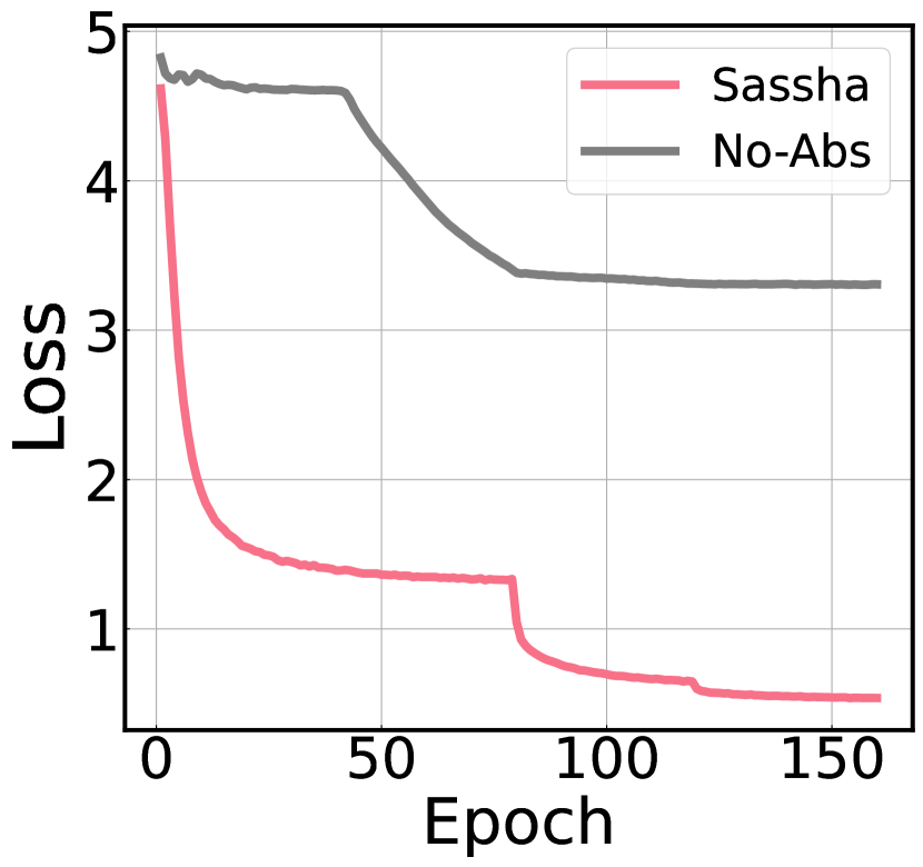
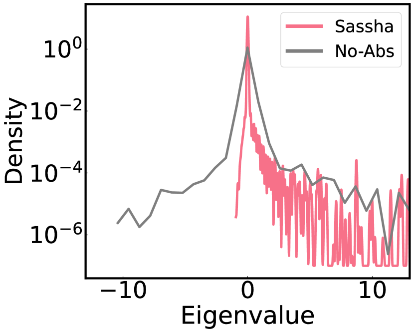
We observe how the absolute function influences the training process to avoid convergence to a critical solution that could result in sub-optimal performance. We train ResNet-32 on CIFAR-100 using Sassha without the absolute function (No-Abs) and compare the resulting training loss to that of the original Sassha. We also plot the Hessian eigenspectrum of the found solution via the Lanczos algorithm (Yao et al., 2020) to determine whether the found solution corresponds to a minimum or a saddle point. The results are illustrated in Figure˜6. We can see that without the absolute function, the training loss converges to a sub-optimal solution, where the prevalent negative values in the diagonal Hessian distribution indicate it as a saddle point. This shows the necessity of the absolute function for preventing convergence to these critical regions.

Appendix F Validation Loss Curve for Vision Task

Refer to caption
Refer to caption
Refer to caption
Refer to caption
Refer to caption
Refer to caption
Figure 7: Validation loss curve of Sassha, SGD, AdaHessian, AdamW, and Sophia-H on various image classification models and tasks. Sassha outperforms all first-order and second-order baseline methods.

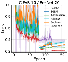
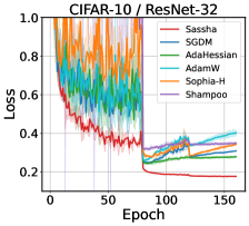
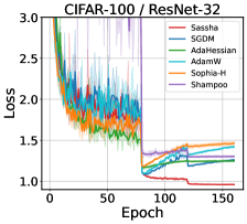
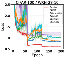
The experimental results in Figure˜7 demonstrate better generalization capability of Sassha over the related methods. Across all datasets and model architectures, our method consistently achieves the lowest validation loss, indicative of its enhanced ability to generalize from training to validation data effectively. This robust performance of Sassha underscores its potential as a leading optimization method for various deep learning applications, particularly in image classification.

Appendix G Comparison with First-order Baselines with Given More Training Budget than Sassha

We train SGD and AdamW for twice as many epochs as Sassha and compare their final validation accuracies. The results are presented in Table˜15. Despite this extended training budget, these first-order methods fall short of the performance attained with Sassha, demonstrating their limited effectiveness compared to Sassha. We attribute this outcome to Sassha reaching a flatter and better generalizing solution along with stable preconditioning, which together enables consistent outperformance over first-order baselines.

Table 15: Performance comparison of Sassha against SGD and AdamW with twice the epoch allocation. Sassha achieves better results with significantly fewer epochs.
RN20 - CIFAR-10 RN32 - CIFAR-10 RN32 - CIFAR-100 WRN28 - CIFAR-100 RN50 - ImageNet ViT_s - ImageNet
Acc (epoch) Acc (epoch) Acc (epoch) Acc (epoch) Acc (epoch) Acc (epoch)
SGD $92.62$ (320e) $93.43$ (320e) $69.93$ (320e) $80.50$ (400e) $75.90$ (180e) $63.64$ (180e)
AdamW $92.55$ (320e) $92.97$ (320e) $69.50$ (320e) $79.46$ (400e) $75.57$ (180e) $66.97$ (180e)
Sassha 92.98 (160e) 94.09 (160e) 72.14 (160e) 83.54 (200e) 76.43 (90e) 69.20 (90e)

Appendix H Effectiveness of Stable Hessian Approximations in Sassha

Table 16: Results of Sophia-H with sharpness minimization.
CIFAR-10 CIFAR-100
ResNet-20 ResNet-32 ResNet-32 WRN-28-10
SAM 92.85±0.0792.85_{{\color[rgb]{0.4,0.4,0.4}\definecolor[named]{pgfstrokecolor}{rgb}{0.4,0.4,0.4}\pgfsys@color@gray@stroke{0.4}\pgfsys@color@gray@fill{0.4}\pm 0.07}} 93.89±0.1393.89_{{\color[rgb]{0.4,0.4,0.4}\definecolor[named]{pgfstrokecolor}{rgb}{0.4,0.4,0.4}\pgfsys@color@gray@stroke{0.4}\pgfsys@color@gray@fill{0.4}\pm 0.13}} 71.99±0.2071.99_{{\color[rgb]{0.4,0.4,0.4}\definecolor[named]{pgfstrokecolor}{rgb}{0.4,0.4,0.4}\pgfsys@color@gray@stroke{0.4}\pgfsys@color@gray@fill{0.4}\pm 0.20}} 83.14±0.1383.14_{{\color[rgb]{0.4,0.4,0.4}\definecolor[named]{pgfstrokecolor}{rgb}{0.4,0.4,0.4}\pgfsys@color@gray@stroke{0.4}\pgfsys@color@gray@fill{0.4}\pm 0.13}}
Sophia-H (with SAM) ${}_{\text{}}$ 92.53±0.3992.53_{{\color[rgb]{0.4,0.4,0.4}\definecolor[named]{pgfstrokecolor}{rgb}{0.4,0.4,0.4}\pgfsys@color@gray@stroke{0.4}\pgfsys@color@gray@fill{0.4}\pm 0.39}} 93.59±0.3193.59_{{\color[rgb]{0.4,0.4,0.4}\definecolor[named]{pgfstrokecolor}{rgb}{0.4,0.4,0.4}\pgfsys@color@gray@stroke{0.4}\pgfsys@color@gray@fill{0.4}\pm 0.31}} 71.31±0.4371.31_{{\color[rgb]{0.4,0.4,0.4}\definecolor[named]{pgfstrokecolor}{rgb}{0.4,0.4,0.4}\pgfsys@color@gray@stroke{0.4}\pgfsys@color@gray@fill{0.4}\pm 0.43}} 80.15±0.3580.15_{{\color[rgb]{0.4,0.4,0.4}\definecolor[named]{pgfstrokecolor}{rgb}{0.4,0.4,0.4}\pgfsys@color@gray@stroke{0.4}\pgfsys@color@gray@fill{0.4}\pm 0.35}}
Sassha 92.98±0.05\textbf{92.98}_{{\color[rgb]{0.4,0.4,0.4}\definecolor[named]{pgfstrokecolor}{rgb}{0.4,0.4,0.4}\pgfsys@color@gray@stroke{0.4}\pgfsys@color@gray@fill{0.4}\pm 0.05}} 94.09±0.24\textbf{94.09}_{{\color[rgb]{0.4,0.4,0.4}\definecolor[named]{pgfstrokecolor}{rgb}{0.4,0.4,0.4}\pgfsys@color@gray@stroke{0.4}\pgfsys@color@gray@fill{0.4}\pm 0.24}} 72.14±0.16\textbf{72.14}_{{\color[rgb]{0.4,0.4,0.4}\definecolor[named]{pgfstrokecolor}{rgb}{0.4,0.4,0.4}\pgfsys@color@gray@stroke{0.4}\pgfsys@color@gray@fill{0.4}\pm 0.16}} 83.54±0.08\textbf{83.54}_{{\color[rgb]{0.4,0.4,0.4}\definecolor[named]{pgfstrokecolor}{rgb}{0.4,0.4,0.4}\pgfsys@color@gray@stroke{0.4}\pgfsys@color@gray@fill{0.4}\pm 0.08}}

We demonstrate limited benefit from naively combining SAM with existing approximate second-order methods without the carefully designed stabilization strategies of Sassha. Precisely, we compare the validation accuracy of Sassha with a simple combination of SAM and Sophia, denoted as Sophia-H (with SAM). We provide results in Table˜16.

We observe that Sophia-H (with SAM) performs worse than SAM, whereas Sassha outperforms both methods, validating the effectiveness of the design choices made in Sassha. We attribute this to the reduced compatibility of Sophia-H with SAM compared to Sassha. First, when curvature is reduced due to SAM, clipping may cause a significant increase in the number of Hessian entries replaced by a very small constant. This situation raises the sensitivity to hyperparameters like the clipping threshold and makes the optimization process more dependent on careful tuning. Conversely, the stable Hessian approximation in Sassha, incorporating the absolute function and square rooting, avoids enforcing hard adjustments to the magnitude or direction of the update vector or to Hessian entries. Instead, it smoothly adjusts Hessian, preserving its structural integrity while mitigating extreme values.

In addition, the use of clipping results in Sophia partially performing signSGD over a subset of parameters (Liu et al., 2024), which may lead to suboptimal convergence in typical situations (Karimireddy et al., 2019).

Appendix I Comparison with Advanced SAM Variants

Thus far, our primary focus has centered on validating the effectiveness of Sassha in the context of approximate second-order optimization. While this remains the principal objective of our study, here we additionally compare Sassha with advanced SAM variants (i.e. ASAM (Kwon et al., 2021), GSAM (Zhuang et al., 2022)) to prove that Sassha is a sensible approach. We also evaluate G-Sassha (Sassha with surrogate gap guided sharpness from (Zhuang et al., 2022)) for fair comparison. The results are represented in Table˜17.

Table 17: Sassha v.s. advanced SAM variants in Image classification.
CIFAR-10 CIFAR-100 ImageNet
ResNet-20 ResNet-32 ResNet-32 WRN-28-10 ResNet-50 ViT-s-32
ASAM 92.96±0.2592.96_{{\color[rgb]{0.4,0.4,0.4}\definecolor[named]{pgfstrokecolor}{rgb}{0.4,0.4,0.4}\pgfsys@color@gray@stroke{0.4}\pgfsys@color@gray@fill{0.4}\pm 0.25}} 93.85±0.1593.85_{{\color[rgb]{0.4,0.4,0.4}\definecolor[named]{pgfstrokecolor}{rgb}{0.4,0.4,0.4}\pgfsys@color@gray@stroke{0.4}\pgfsys@color@gray@fill{0.4}\pm 0.15}} 72.02±0.2872.02_{{\color[rgb]{0.4,0.4,0.4}\definecolor[named]{pgfstrokecolor}{rgb}{0.4,0.4,0.4}\pgfsys@color@gray@stroke{0.4}\pgfsys@color@gray@fill{0.4}\pm 0.28}} 83.39±0.0683.39_{{\color[rgb]{0.4,0.4,0.4}\definecolor[named]{pgfstrokecolor}{rgb}{0.4,0.4,0.4}\pgfsys@color@gray@stroke{0.4}\pgfsys@color@gray@fill{0.4}\pm 0.06}} 76.54±0.1576.54_{{\color[rgb]{0.4,0.4,0.4}\definecolor[named]{pgfstrokecolor}{rgb}{0.4,0.4,0.4}\pgfsys@color@gray@stroke{0.4}\pgfsys@color@gray@fill{0.4}\pm 0.15}} 68.26±0.3668.26_{{\color[rgb]{0.4,0.4,0.4}\definecolor[named]{pgfstrokecolor}{rgb}{0.4,0.4,0.4}\pgfsys@color@gray@stroke{0.4}\pgfsys@color@gray@fill{0.4}\pm 0.36}}
GSAM 92.72±0.3992.72_{{\color[rgb]{0.4,0.4,0.4}\definecolor[named]{pgfstrokecolor}{rgb}{0.4,0.4,0.4}\pgfsys@color@gray@stroke{0.4}\pgfsys@color@gray@fill{0.4}\pm 0.39}} 93.76±0.3193.76_{{\color[rgb]{0.4,0.4,0.4}\definecolor[named]{pgfstrokecolor}{rgb}{0.4,0.4,0.4}\pgfsys@color@gray@stroke{0.4}\pgfsys@color@gray@fill{0.4}\pm 0.31}} 72.10±0.4372.10_{{\color[rgb]{0.4,0.4,0.4}\definecolor[named]{pgfstrokecolor}{rgb}{0.4,0.4,0.4}\pgfsys@color@gray@stroke{0.4}\pgfsys@color@gray@fill{0.4}\pm 0.43}} 83.21±0.3983.21_{{\color[rgb]{0.4,0.4,0.4}\definecolor[named]{pgfstrokecolor}{rgb}{0.4,0.4,0.4}\pgfsys@color@gray@stroke{0.4}\pgfsys@color@gray@fill{0.4}\pm 0.39}} 76.45±0.2276.45_{{\color[rgb]{0.4,0.4,0.4}\definecolor[named]{pgfstrokecolor}{rgb}{0.4,0.4,0.4}\pgfsys@color@gray@stroke{0.4}\pgfsys@color@gray@fill{0.4}\pm 0.22}} 69.60±0.1669.60_{{\color[rgb]{0.4,0.4,0.4}\definecolor[named]{pgfstrokecolor}{rgb}{0.4,0.4,0.4}\pgfsys@color@gray@stroke{0.4}\pgfsys@color@gray@fill{0.4}\pm 0.16}}
Sassha 92.98±0.05\textbf{92.98}_{{\color[rgb]{0.4,0.4,0.4}\definecolor[named]{pgfstrokecolor}{rgb}{0.4,0.4,0.4}\pgfsys@color@gray@stroke{0.4}\pgfsys@color@gray@fill{0.4}\pm 0.05}} 94.09±0.2494.09_{{\color[rgb]{0.4,0.4,0.4}\definecolor[named]{pgfstrokecolor}{rgb}{0.4,0.4,0.4}\pgfsys@color@gray@stroke{0.4}\pgfsys@color@gray@fill{0.4}\pm 0.24}} 72.14±0.1672.14_{{\color[rgb]{0.4,0.4,0.4}\definecolor[named]{pgfstrokecolor}{rgb}{0.4,0.4,0.4}\pgfsys@color@gray@stroke{0.4}\pgfsys@color@gray@fill{0.4}\pm 0.16}} 83.54±0.0883.54_{{\color[rgb]{0.4,0.4,0.4}\definecolor[named]{pgfstrokecolor}{rgb}{0.4,0.4,0.4}\pgfsys@color@gray@stroke{0.4}\pgfsys@color@gray@fill{0.4}\pm 0.08}} 76.43±0.1876.43_{{\color[rgb]{0.4,0.4,0.4}\definecolor[named]{pgfstrokecolor}{rgb}{0.4,0.4,0.4}\pgfsys@color@gray@stroke{0.4}\pgfsys@color@gray@fill{0.4}\pm 0.18}} 69.20±0.3069.20_{{\color[rgb]{0.4,0.4,0.4}\definecolor[named]{pgfstrokecolor}{rgb}{0.4,0.4,0.4}\pgfsys@color@gray@stroke{0.4}\pgfsys@color@gray@fill{0.4}\pm 0.30}}
G-Sassha 92.94±0.1892.94_{{\color[rgb]{0.4,0.4,0.4}\definecolor[named]{pgfstrokecolor}{rgb}{0.4,0.4,0.4}\pgfsys@color@gray@stroke{0.4}\pgfsys@color@gray@fill{0.4}\pm 0.18}} 94.15±0.12\textbf{94.15}_{{\color[rgb]{0.4,0.4,0.4}\definecolor[named]{pgfstrokecolor}{rgb}{0.4,0.4,0.4}\pgfsys@color@gray@stroke{0.4}\pgfsys@color@gray@fill{0.4}\pm 0.12}} 72.18±0.52\textbf{72.18}_{{\color[rgb]{0.4,0.4,0.4}\definecolor[named]{pgfstrokecolor}{rgb}{0.4,0.4,0.4}\pgfsys@color@gray@stroke{0.4}\pgfsys@color@gray@fill{0.4}\pm 0.52}} 83.56±0.27\textbf{83.56}_{{\color[rgb]{0.4,0.4,0.4}\definecolor[named]{pgfstrokecolor}{rgb}{0.4,0.4,0.4}\pgfsys@color@gray@stroke{0.4}\pgfsys@color@gray@fill{0.4}\pm 0.27}} 76.66±0.23\textbf{76.66}_{{\color[rgb]{0.4,0.4,0.4}\definecolor[named]{pgfstrokecolor}{rgb}{0.4,0.4,0.4}\pgfsys@color@gray@stroke{0.4}\pgfsys@color@gray@fill{0.4}\pm 0.23}} 69.67±0.14\textbf{69.67}_{{\color[rgb]{0.4,0.4,0.4}\definecolor[named]{pgfstrokecolor}{rgb}{0.4,0.4,0.4}\pgfsys@color@gray@stroke{0.4}\pgfsys@color@gray@fill{0.4}\pm 0.14}}

We find that Sassha is competitive with these advanced SAM variants. However, we note clearly that those SAM variants require considerably more hyperparameter tuning to achieve generalization performance comparable to Sassha. For example, GSAM introduces an additional hyperparameter $\alpha$, demanding as much tuning effort as tuning $\rho$. Similarly, ASAM, as noted by its authors, typically necessitates exploring a broader $\rho$ range, as its appropriate value is approximately 10 times larger than that of SAM. In our setup, tuning GSAM and ASAM involved $4.5\times\sim 15.75\times$ and $3\times\sim 8\times$ larger search grids compared to Sassha, respectively. We provide detailed setup and hyperparameter search space below.

Setup and Search space. For ResNet, we use SGD as the base methods for ASAM and GSAM, while for ViT, AdamW with gradient clipping set to 1.0 serves as the base methods. For all models, typical cross entropy loss is used (not label-smoothing cross entropy), and the best learning rate and weight decay of the base methods are selected in experiments with ASAM and GSAM. All algorithms are evaluated with constant $\rho$ (without scheduling). For learning rate schedule, we apply multi-step decay with a decay rate of 0.1 for ResNet on CIFAR, and use cosine learning rate decay with 8 warm-up epochs for ViTs.

ResNet/CIFAR ResNet/ImageNet ViT/ImageNet
    $\rho$ $\{0.01,0.05,0.1,0.15,0.2,0.25,0.3,0.35,0.4\}$ $\{0.01,0.05,0.1,0.15,0.2,0.25,0.3\}$ $\{0.1,0.2,0.3,0.4,0.5,0.6\}$
    $\alpha$ $\{0.01,0.05,0.1,0.15,0.2,0.25,0.3\}$ $\{0.01,0.05,0.1,0.15,0.2\}$ $\{0.1,0.2,0.3\}$
Table 18: Hyperparameter search space for GSAM and G-Sassha
ResNet/CIFAR ImageNet
    $\rho$ $\Bigl{\{}\begin{subarray}{c}0.01,0.05,0.1,0.15,0.2,0.25,0.3,0.4,0.5,0.6,0.7,0.8,0.9,1,\\ 1.1,1.2,1.3,1.4,1.5,1.6,1.7,1.8,1.9,2,2.5,3,3.5,4,4.5,5,5.5,6\end{subarray}\Bigr{\}}$ $\{0.1,0.15,0.2,0.3,0.4,0.5,0.6,0.7,0.8,0.9,1,1.5,2\}$
Table 19: Hyperparameter search space for ASAM

Appendix J Additional Label Noise Experiments

Table 20: Robustness to label noise. Here we measure the validation accuracy under various levels of label noise using ResNet-32 trained on CIFAR-100 and CIFAR-10. Sassha shows much robust performance under label noise.
CIFAR-10 CIFAR-100
Noise level 0% 20% 40% 60% 0% 20% 40% 60%
SGD 92.69±0.0692.69_{{\color[rgb]{0.4,0.4,0.4}\definecolor[named]{pgfstrokecolor}{rgb}{0.4,0.4,0.4}\pgfsys@color@gray@stroke{0.4}\pgfsys@color@gray@fill{0.4}\pm 0.06}} 89.91±0.8789.91_{{\color[rgb]{0.4,0.4,0.4}\definecolor[named]{pgfstrokecolor}{rgb}{0.4,0.4,0.4}\pgfsys@color@gray@stroke{0.4}\pgfsys@color@gray@fill{0.4}\pm 0.87}} 87.26±0.4087.26_{{\color[rgb]{0.4,0.4,0.4}\definecolor[named]{pgfstrokecolor}{rgb}{0.4,0.4,0.4}\pgfsys@color@gray@stroke{0.4}\pgfsys@color@gray@fill{0.4}\pm 0.40}} 82.72±1.5982.72_{{\color[rgb]{0.4,0.4,0.4}\definecolor[named]{pgfstrokecolor}{rgb}{0.4,0.4,0.4}\pgfsys@color@gray@stroke{0.4}\pgfsys@color@gray@fill{0.4}\pm 1.59}} 69.32±0.1969.32_{{\color[rgb]{0.4,0.4,0.4}\definecolor[named]{pgfstrokecolor}{rgb}{0.4,0.4,0.4}\pgfsys@color@gray@stroke{0.4}\pgfsys@color@gray@fill{0.4}\pm 0.19}} 62.18±0.0662.18_{{\color[rgb]{0.4,0.4,0.4}\definecolor[named]{pgfstrokecolor}{rgb}{0.4,0.4,0.4}\pgfsys@color@gray@stroke{0.4}\pgfsys@color@gray@fill{0.4}\pm 0.06}} 55.78±0.5555.78_{{\color[rgb]{0.4,0.4,0.4}\definecolor[named]{pgfstrokecolor}{rgb}{0.4,0.4,0.4}\pgfsys@color@gray@stroke{0.4}\pgfsys@color@gray@fill{0.4}\pm 0.55}} 45.53±0.7845.53_{{\color[rgb]{0.4,0.4,0.4}\definecolor[named]{pgfstrokecolor}{rgb}{0.4,0.4,0.4}\pgfsys@color@gray@stroke{0.4}\pgfsys@color@gray@fill{0.4}\pm 0.78}}
SAM ${}_{\text{SGD}}$ 93.89±0.1393.89_{{\color[rgb]{0.4,0.4,0.4}\definecolor[named]{pgfstrokecolor}{rgb}{0.4,0.4,0.4}\pgfsys@color@gray@stroke{0.4}\pgfsys@color@gray@fill{0.4}\pm 0.13}} 92.27±0.1492.27_{{\color[rgb]{0.4,0.4,0.4}\definecolor[named]{pgfstrokecolor}{rgb}{0.4,0.4,0.4}\pgfsys@color@gray@stroke{0.4}\pgfsys@color@gray@fill{0.4}\pm 0.14}} 90.11±0.2590.11_{{\color[rgb]{0.4,0.4,0.4}\definecolor[named]{pgfstrokecolor}{rgb}{0.4,0.4,0.4}\pgfsys@color@gray@stroke{0.4}\pgfsys@color@gray@fill{0.4}\pm 0.25}} 85.79±0.3085.79_{{\color[rgb]{0.4,0.4,0.4}\definecolor[named]{pgfstrokecolor}{rgb}{0.4,0.4,0.4}\pgfsys@color@gray@stroke{0.4}\pgfsys@color@gray@fill{0.4}\pm 0.30}} 71.99±0.2071.99_{{\color[rgb]{0.4,0.4,0.4}\definecolor[named]{pgfstrokecolor}{rgb}{0.4,0.4,0.4}\pgfsys@color@gray@stroke{0.4}\pgfsys@color@gray@fill{0.4}\pm 0.20}} 65.53±0.1165.53_{{\color[rgb]{0.4,0.4,0.4}\definecolor[named]{pgfstrokecolor}{rgb}{0.4,0.4,0.4}\pgfsys@color@gray@stroke{0.4}\pgfsys@color@gray@fill{0.4}\pm 0.11}} 61.20±0.1761.20_{{\color[rgb]{0.4,0.4,0.4}\definecolor[named]{pgfstrokecolor}{rgb}{0.4,0.4,0.4}\pgfsys@color@gray@stroke{0.4}\pgfsys@color@gray@fill{0.4}\pm 0.17}} 51.93±0.4751.93_{{\color[rgb]{0.4,0.4,0.4}\definecolor[named]{pgfstrokecolor}{rgb}{0.4,0.4,0.4}\pgfsys@color@gray@stroke{0.4}\pgfsys@color@gray@fill{0.4}\pm 0.47}}
AdaHessian 92.48±0.1592.48_{{\color[rgb]{0.4,0.4,0.4}\definecolor[named]{pgfstrokecolor}{rgb}{0.4,0.4,0.4}\pgfsys@color@gray@stroke{0.4}\pgfsys@color@gray@fill{0.4}\pm 0.15}} 90.11±0.0190.11_{{\color[rgb]{0.4,0.4,0.4}\definecolor[named]{pgfstrokecolor}{rgb}{0.4,0.4,0.4}\pgfsys@color@gray@stroke{0.4}\pgfsys@color@gray@fill{0.4}\pm 0.01}} 86.88±0.0486.88_{{\color[rgb]{0.4,0.4,0.4}\definecolor[named]{pgfstrokecolor}{rgb}{0.4,0.4,0.4}\pgfsys@color@gray@stroke{0.4}\pgfsys@color@gray@fill{0.4}\pm 0.04}} 83.25±0.0183.25_{{\color[rgb]{0.4,0.4,0.4}\definecolor[named]{pgfstrokecolor}{rgb}{0.4,0.4,0.4}\pgfsys@color@gray@stroke{0.4}\pgfsys@color@gray@fill{0.4}\pm 0.01}} 68.06±0.2268.06_{{\color[rgb]{0.4,0.4,0.4}\definecolor[named]{pgfstrokecolor}{rgb}{0.4,0.4,0.4}\pgfsys@color@gray@stroke{0.4}\pgfsys@color@gray@fill{0.4}\pm 0.22}} 63.06±0.2563.06_{{\color[rgb]{0.4,0.4,0.4}\definecolor[named]{pgfstrokecolor}{rgb}{0.4,0.4,0.4}\pgfsys@color@gray@stroke{0.4}\pgfsys@color@gray@fill{0.4}\pm 0.25}} 58.37±0.1358.37_{{\color[rgb]{0.4,0.4,0.4}\definecolor[named]{pgfstrokecolor}{rgb}{0.4,0.4,0.4}\pgfsys@color@gray@stroke{0.4}\pgfsys@color@gray@fill{0.4}\pm 0.13}} 46.02±1.9646.02_{{\color[rgb]{0.4,0.4,0.4}\definecolor[named]{pgfstrokecolor}{rgb}{0.4,0.4,0.4}\pgfsys@color@gray@stroke{0.4}\pgfsys@color@gray@fill{0.4}\pm 1.96}}
Sophia-H 91.99±0.0891.99_{{\color[rgb]{0.4,0.4,0.4}\definecolor[named]{pgfstrokecolor}{rgb}{0.4,0.4,0.4}\pgfsys@color@gray@stroke{0.4}\pgfsys@color@gray@fill{0.4}\pm 0.08}} 89.93±0.0189.93_{{\color[rgb]{0.4,0.4,0.4}\definecolor[named]{pgfstrokecolor}{rgb}{0.4,0.4,0.4}\pgfsys@color@gray@stroke{0.4}\pgfsys@color@gray@fill{0.4}\pm 0.01}} 87.30±0.5187.30_{{\color[rgb]{0.4,0.4,0.4}\definecolor[named]{pgfstrokecolor}{rgb}{0.4,0.4,0.4}\pgfsys@color@gray@stroke{0.4}\pgfsys@color@gray@fill{0.4}\pm 0.51}} 82.78±1.4382.78_{{\color[rgb]{0.4,0.4,0.4}\definecolor[named]{pgfstrokecolor}{rgb}{0.4,0.4,0.4}\pgfsys@color@gray@stroke{0.4}\pgfsys@color@gray@fill{0.4}\pm 1.43}} 67.76±0.3767.76_{{\color[rgb]{0.4,0.4,0.4}\definecolor[named]{pgfstrokecolor}{rgb}{0.4,0.4,0.4}\pgfsys@color@gray@stroke{0.4}\pgfsys@color@gray@fill{0.4}\pm 0.37}} 62.34±0.4762.34_{{\color[rgb]{0.4,0.4,0.4}\definecolor[named]{pgfstrokecolor}{rgb}{0.4,0.4,0.4}\pgfsys@color@gray@stroke{0.4}\pgfsys@color@gray@fill{0.4}\pm 0.47}} 56.54±0.2856.54_{{\color[rgb]{0.4,0.4,0.4}\definecolor[named]{pgfstrokecolor}{rgb}{0.4,0.4,0.4}\pgfsys@color@gray@stroke{0.4}\pgfsys@color@gray@fill{0.4}\pm 0.28}} 45.37±0.2745.37_{{\color[rgb]{0.4,0.4,0.4}\definecolor[named]{pgfstrokecolor}{rgb}{0.4,0.4,0.4}\pgfsys@color@gray@stroke{0.4}\pgfsys@color@gray@fill{0.4}\pm 0.27}}
Shampoo 90.23±0.8390.23_{{\color[rgb]{0.4,0.4,0.4}\definecolor[named]{pgfstrokecolor}{rgb}{0.4,0.4,0.4}\pgfsys@color@gray@stroke{0.4}\pgfsys@color@gray@fill{0.4}\pm 0.83}} 88.14±0.2988.14_{{\color[rgb]{0.4,0.4,0.4}\definecolor[named]{pgfstrokecolor}{rgb}{0.4,0.4,0.4}\pgfsys@color@gray@stroke{0.4}\pgfsys@color@gray@fill{0.4}\pm 0.29}} 85.15±0.6185.15_{{\color[rgb]{0.4,0.4,0.4}\definecolor[named]{pgfstrokecolor}{rgb}{0.4,0.4,0.4}\pgfsys@color@gray@stroke{0.4}\pgfsys@color@gray@fill{0.4}\pm 0.61}} 81.16±0.3081.16_{{\color[rgb]{0.4,0.4,0.4}\definecolor[named]{pgfstrokecolor}{rgb}{0.4,0.4,0.4}\pgfsys@color@gray@stroke{0.4}\pgfsys@color@gray@fill{0.4}\pm 0.30}} 64.08±0.4664.08_{{\color[rgb]{0.4,0.4,0.4}\definecolor[named]{pgfstrokecolor}{rgb}{0.4,0.4,0.4}\pgfsys@color@gray@stroke{0.4}\pgfsys@color@gray@fill{0.4}\pm 0.46}} 58.85±0.6658.85_{{\color[rgb]{0.4,0.4,0.4}\definecolor[named]{pgfstrokecolor}{rgb}{0.4,0.4,0.4}\pgfsys@color@gray@stroke{0.4}\pgfsys@color@gray@fill{0.4}\pm 0.66}} 53.82±0.7153.82_{{\color[rgb]{0.4,0.4,0.4}\definecolor[named]{pgfstrokecolor}{rgb}{0.4,0.4,0.4}\pgfsys@color@gray@stroke{0.4}\pgfsys@color@gray@fill{0.4}\pm 0.71}} 42.91±0.9942.91_{{\color[rgb]{0.4,0.4,0.4}\definecolor[named]{pgfstrokecolor}{rgb}{0.4,0.4,0.4}\pgfsys@color@gray@stroke{0.4}\pgfsys@color@gray@fill{0.4}\pm 0.99}}
Sassha 94.09±0.24\textbf{94.09}_{{\color[rgb]{0.4,0.4,0.4}\definecolor[named]{pgfstrokecolor}{rgb}{0.4,0.4,0.4}\pgfsys@color@gray@stroke{0.4}\pgfsys@color@gray@fill{0.4}\pm 0.24}} 92.49±0.11\textbf{92.49}_{{\color[rgb]{0.4,0.4,0.4}\definecolor[named]{pgfstrokecolor}{rgb}{0.4,0.4,0.4}\pgfsys@color@gray@stroke{0.4}\pgfsys@color@gray@fill{0.4}\pm 0.11}} 90.29±0.11\textbf{90.29}_{{\color[rgb]{0.4,0.4,0.4}\definecolor[named]{pgfstrokecolor}{rgb}{0.4,0.4,0.4}\pgfsys@color@gray@stroke{0.4}\pgfsys@color@gray@fill{0.4}\pm 0.11}} 86.50±0.08\textbf{86.50}_{{\color[rgb]{0.4,0.4,0.4}\definecolor[named]{pgfstrokecolor}{rgb}{0.4,0.4,0.4}\pgfsys@color@gray@stroke{0.4}\pgfsys@color@gray@fill{0.4}\pm 0.08}} 72.14±0.16\textbf{72.14}_{{\color[rgb]{0.4,0.4,0.4}\definecolor[named]{pgfstrokecolor}{rgb}{0.4,0.4,0.4}\pgfsys@color@gray@stroke{0.4}\pgfsys@color@gray@fill{0.4}\pm 0.16}} 66.78±0.47\textbf{66.78}_{{\color[rgb]{0.4,0.4,0.4}\definecolor[named]{pgfstrokecolor}{rgb}{0.4,0.4,0.4}\pgfsys@color@gray@stroke{0.4}\pgfsys@color@gray@fill{0.4}\pm 0.47}} 61.97±0.27\textbf{61.97}_{{\color[rgb]{0.4,0.4,0.4}\definecolor[named]{pgfstrokecolor}{rgb}{0.4,0.4,0.4}\pgfsys@color@gray@stroke{0.4}\pgfsys@color@gray@fill{0.4}\pm 0.27}} 53.98±0.57\textbf{53.98}_{{\color[rgb]{0.4,0.4,0.4}\definecolor[named]{pgfstrokecolor}{rgb}{0.4,0.4,0.4}\pgfsys@color@gray@stroke{0.4}\pgfsys@color@gray@fill{0.4}\pm 0.57}}

Appendix K M-Sassha: Efficient Perturbation

Having explored techniques to reduce the computational cost of second-order methods, here we consider employing techniques to alleviate the additional gradient computation in sharpness-minimization. Prior works have suggested different ways to reduce this computational overhead including infrequent computations (Liu et al., 2022), use of sparse perturbations (Mi et al., 2022), or computing with selective weight and data (Du et al., 2022a). In particular, we employ the approaches of Becker et al. (2024), which uses the normalized negative momentum as the perturbation:

$$\epsilon^{\star}_{t}=\rho\frac{m_{t-1}}{\|m_{t-1}\|_{2}},$$ (9)

which entirely eliminates the need for additional gradient computation with similar generalization improvement as the original SAM. We call this low-computation alternative as M-Sassha and evaluate this across vision, language, and label noise tasks, as we did in the main sections. The results are presented in Tables˜21, 22 and 23, respectively.

Despite having a computational cost comparable to first-order methods like SGD and Adam, and significantly lower than approximate second-order methods, M-Sassha demonstrates superior performance over both first-order and second-order approaches. In image classification, M-Sassha proves more effective than the best-performing approximate second-order methods by 2% on CIFAR-100 with ResNet-32 and by 2.5% with ResNet-50, while also exceeding AdamW by approximately 1.6% on ViT. For language pretraining, it attains a test perplexity that is 22 points lower than the second-best performinig Sophia-H and outperforms AdamW in nearly all language tasks. Lastly, M-Sassha surpasses other methods across all noise levels, proving highly resilient in the presence of extreme label noise. These results reaffirm the effectiveness and consistency of our well-engineered design choices, which enable the stable integration of efficient sharpness minimization into second-order optimization while retaining its benefits.

Table 21: M-Sassha v.s. baselines in image classification. M-Sassha shows superior performance.
CIFAR-10 CIFAR-100 ImageNet
Category Method ResNet-20 ResNet-32 ResNet-32 WRN-28-10 ResNet-50 ViT-s-32
First-order SGD 92.03±0.3292.03_{{\color[rgb]{0.4,0.4,0.4}\definecolor[named]{pgfstrokecolor}{rgb}{0.4,0.4,0.4}\pgfsys@color@gray@stroke{0.4}\pgfsys@color@gray@fill{0.4}\pm 0.32}} 92.69±0.0692.69_{{\color[rgb]{0.4,0.4,0.4}\definecolor[named]{pgfstrokecolor}{rgb}{0.4,0.4,0.4}\pgfsys@color@gray@stroke{0.4}\pgfsys@color@gray@fill{0.4}\pm 0.06}} 69.32±0.1969.32_{{\color[rgb]{0.4,0.4,0.4}\definecolor[named]{pgfstrokecolor}{rgb}{0.4,0.4,0.4}\pgfsys@color@gray@stroke{0.4}\pgfsys@color@gray@fill{0.4}\pm 0.19}} 80.06±0.1580.06_{{\color[rgb]{0.4,0.4,0.4}\definecolor[named]{pgfstrokecolor}{rgb}{0.4,0.4,0.4}\pgfsys@color@gray@stroke{0.4}\pgfsys@color@gray@fill{0.4}\pm 0.15}} 75.58±0.0575.58_{{\color[rgb]{0.4,0.4,0.4}\definecolor[named]{pgfstrokecolor}{rgb}{0.4,0.4,0.4}\pgfsys@color@gray@stroke{0.4}\pgfsys@color@gray@fill{0.4}\pm 0.05}} 62.90±0.3662.90_{{\color[rgb]{0.4,0.4,0.4}\definecolor[named]{pgfstrokecolor}{rgb}{0.4,0.4,0.4}\pgfsys@color@gray@stroke{0.4}\pgfsys@color@gray@fill{0.4}\pm 0.36}}
AdamW 92.04±0.1192.04_{{\color[rgb]{0.4,0.4,0.4}\definecolor[named]{pgfstrokecolor}{rgb}{0.4,0.4,0.4}\pgfsys@color@gray@stroke{0.4}\pgfsys@color@gray@fill{0.4}\pm 0.11}} 92.42±0.1392.42_{{\color[rgb]{0.4,0.4,0.4}\definecolor[named]{pgfstrokecolor}{rgb}{0.4,0.4,0.4}\pgfsys@color@gray@stroke{0.4}\pgfsys@color@gray@fill{0.4}\pm 0.13}} 68.78±0.2268.78_{{\color[rgb]{0.4,0.4,0.4}\definecolor[named]{pgfstrokecolor}{rgb}{0.4,0.4,0.4}\pgfsys@color@gray@stroke{0.4}\pgfsys@color@gray@fill{0.4}\pm 0.22}} 79.09±0.3579.09_{{\color[rgb]{0.4,0.4,0.4}\definecolor[named]{pgfstrokecolor}{rgb}{0.4,0.4,0.4}\pgfsys@color@gray@stroke{0.4}\pgfsys@color@gray@fill{0.4}\pm 0.35}} 75.38±0.0875.38_{{\color[rgb]{0.4,0.4,0.4}\definecolor[named]{pgfstrokecolor}{rgb}{0.4,0.4,0.4}\pgfsys@color@gray@stroke{0.4}\pgfsys@color@gray@fill{0.4}\pm 0.08}} 66.46±0.1566.46_{{\color[rgb]{0.4,0.4,0.4}\definecolor[named]{pgfstrokecolor}{rgb}{0.4,0.4,0.4}\pgfsys@color@gray@stroke{0.4}\pgfsys@color@gray@fill{0.4}\pm 0.15}}
Second-order AdaHessian 92.00±0.1792.00_{{\color[rgb]{0.4,0.4,0.4}\definecolor[named]{pgfstrokecolor}{rgb}{0.4,0.4,0.4}\pgfsys@color@gray@stroke{0.4}\pgfsys@color@gray@fill{0.4}\pm 0.17}} 92.48±0.1592.48_{{\color[rgb]{0.4,0.4,0.4}\definecolor[named]{pgfstrokecolor}{rgb}{0.4,0.4,0.4}\pgfsys@color@gray@stroke{0.4}\pgfsys@color@gray@fill{0.4}\pm 0.15}} 68.06±0.2268.06_{{\color[rgb]{0.4,0.4,0.4}\definecolor[named]{pgfstrokecolor}{rgb}{0.4,0.4,0.4}\pgfsys@color@gray@stroke{0.4}\pgfsys@color@gray@fill{0.4}\pm 0.22}} 76.92±0.2676.92_{{\color[rgb]{0.4,0.4,0.4}\definecolor[named]{pgfstrokecolor}{rgb}{0.4,0.4,0.4}\pgfsys@color@gray@stroke{0.4}\pgfsys@color@gray@fill{0.4}\pm 0.26}} 73.64±0.1673.64_{{\color[rgb]{0.4,0.4,0.4}\definecolor[named]{pgfstrokecolor}{rgb}{0.4,0.4,0.4}\pgfsys@color@gray@stroke{0.4}\pgfsys@color@gray@fill{0.4}\pm 0.16}} 66.42±0.2366.42_{{\color[rgb]{0.4,0.4,0.4}\definecolor[named]{pgfstrokecolor}{rgb}{0.4,0.4,0.4}\pgfsys@color@gray@stroke{0.4}\pgfsys@color@gray@fill{0.4}\pm 0.23}}
Sophia-H 91.81±0.2791.81_{{\color[rgb]{0.4,0.4,0.4}\definecolor[named]{pgfstrokecolor}{rgb}{0.4,0.4,0.4}\pgfsys@color@gray@stroke{0.4}\pgfsys@color@gray@fill{0.4}\pm 0.27}} 91.99±0.0891.99_{{\color[rgb]{0.4,0.4,0.4}\definecolor[named]{pgfstrokecolor}{rgb}{0.4,0.4,0.4}\pgfsys@color@gray@stroke{0.4}\pgfsys@color@gray@fill{0.4}\pm 0.08}} 67.76±0.3767.76_{{\color[rgb]{0.4,0.4,0.4}\definecolor[named]{pgfstrokecolor}{rgb}{0.4,0.4,0.4}\pgfsys@color@gray@stroke{0.4}\pgfsys@color@gray@fill{0.4}\pm 0.37}} 79.35±0.2479.35_{{\color[rgb]{0.4,0.4,0.4}\definecolor[named]{pgfstrokecolor}{rgb}{0.4,0.4,0.4}\pgfsys@color@gray@stroke{0.4}\pgfsys@color@gray@fill{0.4}\pm 0.24}} 72.06±0.4972.06_{{\color[rgb]{0.4,0.4,0.4}\definecolor[named]{pgfstrokecolor}{rgb}{0.4,0.4,0.4}\pgfsys@color@gray@stroke{0.4}\pgfsys@color@gray@fill{0.4}\pm 0.49}} 62.44±0.3662.44_{{\color[rgb]{0.4,0.4,0.4}\definecolor[named]{pgfstrokecolor}{rgb}{0.4,0.4,0.4}\pgfsys@color@gray@stroke{0.4}\pgfsys@color@gray@fill{0.4}\pm 0.36}}
Shampoo 88.55±0.8388.55_{{\color[rgb]{0.4,0.4,0.4}\definecolor[named]{pgfstrokecolor}{rgb}{0.4,0.4,0.4}\pgfsys@color@gray@stroke{0.4}\pgfsys@color@gray@fill{0.4}\pm 0.83}} 90.23±0.2490.23_{{\color[rgb]{0.4,0.4,0.4}\definecolor[named]{pgfstrokecolor}{rgb}{0.4,0.4,0.4}\pgfsys@color@gray@stroke{0.4}\pgfsys@color@gray@fill{0.4}\pm 0.24}} 64.08±0.4664.08_{{\color[rgb]{0.4,0.4,0.4}\definecolor[named]{pgfstrokecolor}{rgb}{0.4,0.4,0.4}\pgfsys@color@gray@stroke{0.4}\pgfsys@color@gray@fill{0.4}\pm 0.46}} 74.06±1.2874.06_{{\color[rgb]{0.4,0.4,0.4}\definecolor[named]{pgfstrokecolor}{rgb}{0.4,0.4,0.4}\pgfsys@color@gray@stroke{0.4}\pgfsys@color@gray@fill{0.4}\pm 1.28}} $*$ $*$
M-Sassha 92.36±0.23\textbf{92.36}_{{\color[rgb]{0.4,0.4,0.4}\definecolor[named]{pgfstrokecolor}{rgb}{0.4,0.4,0.4}\pgfsys@color@gray@stroke{0.4}\pgfsys@color@gray@fill{0.4}\pm 0.23}} 93.18±0.30\textbf{93.18}_{{\color[rgb]{0.4,0.4,0.4}\definecolor[named]{pgfstrokecolor}{rgb}{0.4,0.4,0.4}\pgfsys@color@gray@stroke{0.4}\pgfsys@color@gray@fill{0.4}\pm 0.30}} 70.93±0.21\textbf{70.93}_{{\color[rgb]{0.4,0.4,0.4}\definecolor[named]{pgfstrokecolor}{rgb}{0.4,0.4,0.4}\pgfsys@color@gray@stroke{0.4}\pgfsys@color@gray@fill{0.4}\pm 0.21}} 81.53±0.27\textbf{81.53}_{{\color[rgb]{0.4,0.4,0.4}\definecolor[named]{pgfstrokecolor}{rgb}{0.4,0.4,0.4}\pgfsys@color@gray@stroke{0.4}\pgfsys@color@gray@fill{0.4}\pm 0.27}} 76.00±0.04\textbf{76.00}_{{\color[rgb]{0.4,0.4,0.4}\definecolor[named]{pgfstrokecolor}{rgb}{0.4,0.4,0.4}\pgfsys@color@gray@stroke{0.4}\pgfsys@color@gray@fill{0.4}\pm 0.04}} 68.04±0.14\textbf{68.04}_{{\color[rgb]{0.4,0.4,0.4}\definecolor[named]{pgfstrokecolor}{rgb}{0.4,0.4,0.4}\pgfsys@color@gray@stroke{0.4}\pgfsys@color@gray@fill{0.4}\pm 0.14}}
Table 22: M-Sassha v.s. baselines in language tasks. For pretraining, M-Sassha achieves the lowest perplexity among all methods. For finetuning, M-Sassha performs better than AdamW and compares competitively with Sophia-H.
Pretrain / GPT1-mini
Wikitext-2
Perplexity
AdamW $175.06$
AdaHessian $407.69$
Sophia-H $157.60$
M-Sassha 125.01
Finetune / SqeezeBERT
SST-2 MRPC STS-B QQP MNLI QNLI RTE
Acc Acc / F1 S/P corr. F1 / Acc mat/m.mat Acc Acc
90.29±0.5290.29_{{\color[rgb]{0.4,0.4,0.4}\definecolor[named]{pgfstrokecolor}{rgb}{0.4,0.4,0.4}\pgfsys@color@gray@stroke{0.4}\pgfsys@color@gray@fill{0.4}\pm 0.52}} 84.56±0.2584.56_{{\color[rgb]{0.4,0.4,0.4}\definecolor[named]{pgfstrokecolor}{rgb}{0.4,0.4,0.4}\pgfsys@color@gray@stroke{0.4}\pgfsys@color@gray@fill{0.4}\pm 0.25}} / 88.99±0.1188.99_{{\color[rgb]{0.4,0.4,0.4}\definecolor[named]{pgfstrokecolor}{rgb}{0.4,0.4,0.4}\pgfsys@color@gray@stroke{0.4}\pgfsys@color@gray@fill{0.4}\pm 0.11}} 88.34±0.1588.34_{{\color[rgb]{0.4,0.4,0.4}\definecolor[named]{pgfstrokecolor}{rgb}{0.4,0.4,0.4}\pgfsys@color@gray@stroke{0.4}\pgfsys@color@gray@fill{0.4}\pm 0.15}} / 88.48±0.2088.48_{{\color[rgb]{0.4,0.4,0.4}\definecolor[named]{pgfstrokecolor}{rgb}{0.4,0.4,0.4}\pgfsys@color@gray@stroke{0.4}\pgfsys@color@gray@fill{0.4}\pm 0.20}} 89.92±0.0589.92_{{\color[rgb]{0.4,0.4,0.4}\definecolor[named]{pgfstrokecolor}{rgb}{0.4,0.4,0.4}\pgfsys@color@gray@stroke{0.4}\pgfsys@color@gray@fill{0.4}\pm 0.05}} / 86.58±0.1186.58_{{\color[rgb]{0.4,0.4,0.4}\definecolor[named]{pgfstrokecolor}{rgb}{0.4,0.4,0.4}\pgfsys@color@gray@stroke{0.4}\pgfsys@color@gray@fill{0.4}\pm 0.11}} 81.22±0.0781.22_{{\color[rgb]{0.4,0.4,0.4}\definecolor[named]{pgfstrokecolor}{rgb}{0.4,0.4,0.4}\pgfsys@color@gray@stroke{0.4}\pgfsys@color@gray@fill{0.4}\pm 0.07}} / 82.26±0.0582.26_{{\color[rgb]{0.4,0.4,0.4}\definecolor[named]{pgfstrokecolor}{rgb}{0.4,0.4,0.4}\pgfsys@color@gray@stroke{0.4}\pgfsys@color@gray@fill{0.4}\pm 0.05}} 89.93±0.1489.93_{{\color[rgb]{0.4,0.4,0.4}\definecolor[named]{pgfstrokecolor}{rgb}{0.4,0.4,0.4}\pgfsys@color@gray@stroke{0.4}\pgfsys@color@gray@fill{0.4}\pm 0.14}} 68.95±0.7268.95_{{\color[rgb]{0.4,0.4,0.4}\definecolor[named]{pgfstrokecolor}{rgb}{0.4,0.4,0.4}\pgfsys@color@gray@stroke{0.4}\pgfsys@color@gray@fill{0.4}\pm 0.72}}
89.64±0.1389.64_{{\color[rgb]{0.4,0.4,0.4}\definecolor[named]{pgfstrokecolor}{rgb}{0.4,0.4,0.4}\pgfsys@color@gray@stroke{0.4}\pgfsys@color@gray@fill{0.4}\pm 0.13}} 79.74±4.0079.74_{{\color[rgb]{0.4,0.4,0.4}\definecolor[named]{pgfstrokecolor}{rgb}{0.4,0.4,0.4}\pgfsys@color@gray@stroke{0.4}\pgfsys@color@gray@fill{0.4}\pm 4.00}} / 85.26±3.5085.26_{{\color[rgb]{0.4,0.4,0.4}\definecolor[named]{pgfstrokecolor}{rgb}{0.4,0.4,0.4}\pgfsys@color@gray@stroke{0.4}\pgfsys@color@gray@fill{0.4}\pm 3.50}} 86.08±4.0486.08_{{\color[rgb]{0.4,0.4,0.4}\definecolor[named]{pgfstrokecolor}{rgb}{0.4,0.4,0.4}\pgfsys@color@gray@stroke{0.4}\pgfsys@color@gray@fill{0.4}\pm 4.04}} / 86.46±4.0686.46_{{\color[rgb]{0.4,0.4,0.4}\definecolor[named]{pgfstrokecolor}{rgb}{0.4,0.4,0.4}\pgfsys@color@gray@stroke{0.4}\pgfsys@color@gray@fill{0.4}\pm 4.06}} 90.37±0.0590.37_{{\color[rgb]{0.4,0.4,0.4}\definecolor[named]{pgfstrokecolor}{rgb}{0.4,0.4,0.4}\pgfsys@color@gray@stroke{0.4}\pgfsys@color@gray@fill{0.4}\pm 0.05}} / 87.07±0.0587.07_{{\color[rgb]{0.4,0.4,0.4}\definecolor[named]{pgfstrokecolor}{rgb}{0.4,0.4,0.4}\pgfsys@color@gray@stroke{0.4}\pgfsys@color@gray@fill{0.4}\pm 0.05}} 81.33±0.1781.33_{{\color[rgb]{0.4,0.4,0.4}\definecolor[named]{pgfstrokecolor}{rgb}{0.4,0.4,0.4}\pgfsys@color@gray@stroke{0.4}\pgfsys@color@gray@fill{0.4}\pm 0.17}} / 82.08±0.0282.08_{{\color[rgb]{0.4,0.4,0.4}\definecolor[named]{pgfstrokecolor}{rgb}{0.4,0.4,0.4}\pgfsys@color@gray@stroke{0.4}\pgfsys@color@gray@fill{0.4}\pm 0.02}} 89.94±0.1289.94_{{\color[rgb]{0.4,0.4,0.4}\definecolor[named]{pgfstrokecolor}{rgb}{0.4,0.4,0.4}\pgfsys@color@gray@stroke{0.4}\pgfsys@color@gray@fill{0.4}\pm 0.12}} 71.00±1.04\textbf{71.00}_{{\color[rgb]{0.4,0.4,0.4}\definecolor[named]{pgfstrokecolor}{rgb}{0.4,0.4,0.4}\pgfsys@color@gray@stroke{0.4}\pgfsys@color@gray@fill{0.4}\pm 1.04}}
90.44±0.46\textbf{90.44}_{{\color[rgb]{0.4,0.4,0.4}\definecolor[named]{pgfstrokecolor}{rgb}{0.4,0.4,0.4}\pgfsys@color@gray@stroke{0.4}\pgfsys@color@gray@fill{0.4}\pm 0.46}} 85.78±1.0785.78_{{\color[rgb]{0.4,0.4,0.4}\definecolor[named]{pgfstrokecolor}{rgb}{0.4,0.4,0.4}\pgfsys@color@gray@stroke{0.4}\pgfsys@color@gray@fill{0.4}\pm 1.07}} / 89.90±0.8289.90_{{\color[rgb]{0.4,0.4,0.4}\definecolor[named]{pgfstrokecolor}{rgb}{0.4,0.4,0.4}\pgfsys@color@gray@stroke{0.4}\pgfsys@color@gray@fill{0.4}\pm 0.82}} 88.17±1.0788.17_{{\color[rgb]{0.4,0.4,0.4}\definecolor[named]{pgfstrokecolor}{rgb}{0.4,0.4,0.4}\pgfsys@color@gray@stroke{0.4}\pgfsys@color@gray@fill{0.4}\pm 1.07}} / 88.53±1.13\textbf{88.53}_{{\color[rgb]{0.4,0.4,0.4}\definecolor[named]{pgfstrokecolor}{rgb}{0.4,0.4,0.4}\pgfsys@color@gray@stroke{0.4}\pgfsys@color@gray@fill{0.4}\pm 1.13}} 90.70±0.0490.70_{{\color[rgb]{0.4,0.4,0.4}\definecolor[named]{pgfstrokecolor}{rgb}{0.4,0.4,0.4}\pgfsys@color@gray@stroke{0.4}\pgfsys@color@gray@fill{0.4}\pm 0.04}} / 87.60±0.0687.60_{{\color[rgb]{0.4,0.4,0.4}\definecolor[named]{pgfstrokecolor}{rgb}{0.4,0.4,0.4}\pgfsys@color@gray@stroke{0.4}\pgfsys@color@gray@fill{0.4}\pm 0.06}} 81.77±0.18\textbf{81.77}_{{\color[rgb]{0.4,0.4,0.4}\definecolor[named]{pgfstrokecolor}{rgb}{0.4,0.4,0.4}\pgfsys@color@gray@stroke{0.4}\pgfsys@color@gray@fill{0.4}\pm 0.18}} / 82.36±0.22\textbf{82.36}_{{\color[rgb]{0.4,0.4,0.4}\definecolor[named]{pgfstrokecolor}{rgb}{0.4,0.4,0.4}\pgfsys@color@gray@stroke{0.4}\pgfsys@color@gray@fill{0.4}\pm 0.22}} 90.12±0.14\textbf{90.12}_{{\color[rgb]{0.4,0.4,0.4}\definecolor[named]{pgfstrokecolor}{rgb}{0.4,0.4,0.4}\pgfsys@color@gray@stroke{0.4}\pgfsys@color@gray@fill{0.4}\pm 0.14}} 70.76±1.4470.76_{{\color[rgb]{0.4,0.4,0.4}\definecolor[named]{pgfstrokecolor}{rgb}{0.4,0.4,0.4}\pgfsys@color@gray@stroke{0.4}\pgfsys@color@gray@fill{0.4}\pm 1.44}}
$90.332_{\pm 0.88}$ $\textbf{87.092}_{\pm 1.98}$ / $\textbf{90.599}_{\pm 1.51}$ $\textbf{88.37}_{\pm 0.04}$ / $88.46_{\pm 0.07}$ $\textbf{90.78}_{\pm 0.05}$ / $\textbf{87.61}_{\pm 0.07}$ $81.42_{\pm 0.19}$ / $81.94_{\pm 0.09}$ $89.84_{\pm 0.22}$ $70.40_{\pm 0.96}$
Table 23: Robustness to label noise. Here we measure the validation accuracy under various levels of label noise using ResNet-32 trained on CIFAR-100 and CIFAR-10. M-Sassha shows much robust performance under label noise.
CIFAR-10 CIFAR-100
Noise level 0% 20% 40% 60% 0% 20% 40% 60%
SGD 92.69±0.0692.69_{{\color[rgb]{0.4,0.4,0.4}\definecolor[named]{pgfstrokecolor}{rgb}{0.4,0.4,0.4}\pgfsys@color@gray@stroke{0.4}\pgfsys@color@gray@fill{0.4}\pm 0.06}} 89.91±0.8789.91_{{\color[rgb]{0.4,0.4,0.4}\definecolor[named]{pgfstrokecolor}{rgb}{0.4,0.4,0.4}\pgfsys@color@gray@stroke{0.4}\pgfsys@color@gray@fill{0.4}\pm 0.87}} 87.26±0.4087.26_{{\color[rgb]{0.4,0.4,0.4}\definecolor[named]{pgfstrokecolor}{rgb}{0.4,0.4,0.4}\pgfsys@color@gray@stroke{0.4}\pgfsys@color@gray@fill{0.4}\pm 0.40}} 82.72±1.5982.72_{{\color[rgb]{0.4,0.4,0.4}\definecolor[named]{pgfstrokecolor}{rgb}{0.4,0.4,0.4}\pgfsys@color@gray@stroke{0.4}\pgfsys@color@gray@fill{0.4}\pm 1.59}} 69.32±0.1969.32_{{\color[rgb]{0.4,0.4,0.4}\definecolor[named]{pgfstrokecolor}{rgb}{0.4,0.4,0.4}\pgfsys@color@gray@stroke{0.4}\pgfsys@color@gray@fill{0.4}\pm 0.19}} 62.18±0.0662.18_{{\color[rgb]{0.4,0.4,0.4}\definecolor[named]{pgfstrokecolor}{rgb}{0.4,0.4,0.4}\pgfsys@color@gray@stroke{0.4}\pgfsys@color@gray@fill{0.4}\pm 0.06}} 55.78±0.5555.78_{{\color[rgb]{0.4,0.4,0.4}\definecolor[named]{pgfstrokecolor}{rgb}{0.4,0.4,0.4}\pgfsys@color@gray@stroke{0.4}\pgfsys@color@gray@fill{0.4}\pm 0.55}} 45.53±0.7845.53_{{\color[rgb]{0.4,0.4,0.4}\definecolor[named]{pgfstrokecolor}{rgb}{0.4,0.4,0.4}\pgfsys@color@gray@stroke{0.4}\pgfsys@color@gray@fill{0.4}\pm 0.78}}
AdaHessian 92.48±0.1592.48_{{\color[rgb]{0.4,0.4,0.4}\definecolor[named]{pgfstrokecolor}{rgb}{0.4,0.4,0.4}\pgfsys@color@gray@stroke{0.4}\pgfsys@color@gray@fill{0.4}\pm 0.15}} 90.11±0.0190.11_{{\color[rgb]{0.4,0.4,0.4}\definecolor[named]{pgfstrokecolor}{rgb}{0.4,0.4,0.4}\pgfsys@color@gray@stroke{0.4}\pgfsys@color@gray@fill{0.4}\pm 0.01}} 86.88±0.0486.88_{{\color[rgb]{0.4,0.4,0.4}\definecolor[named]{pgfstrokecolor}{rgb}{0.4,0.4,0.4}\pgfsys@color@gray@stroke{0.4}\pgfsys@color@gray@fill{0.4}\pm 0.04}} 83.25±0.0183.25_{{\color[rgb]{0.4,0.4,0.4}\definecolor[named]{pgfstrokecolor}{rgb}{0.4,0.4,0.4}\pgfsys@color@gray@stroke{0.4}\pgfsys@color@gray@fill{0.4}\pm 0.01}} 68.06±0.2268.06_{{\color[rgb]{0.4,0.4,0.4}\definecolor[named]{pgfstrokecolor}{rgb}{0.4,0.4,0.4}\pgfsys@color@gray@stroke{0.4}\pgfsys@color@gray@fill{0.4}\pm 0.22}} 63.06±0.2563.06_{{\color[rgb]{0.4,0.4,0.4}\definecolor[named]{pgfstrokecolor}{rgb}{0.4,0.4,0.4}\pgfsys@color@gray@stroke{0.4}\pgfsys@color@gray@fill{0.4}\pm 0.25}} 58.37±0.1358.37_{{\color[rgb]{0.4,0.4,0.4}\definecolor[named]{pgfstrokecolor}{rgb}{0.4,0.4,0.4}\pgfsys@color@gray@stroke{0.4}\pgfsys@color@gray@fill{0.4}\pm 0.13}} 46.02±1.9646.02_{{\color[rgb]{0.4,0.4,0.4}\definecolor[named]{pgfstrokecolor}{rgb}{0.4,0.4,0.4}\pgfsys@color@gray@stroke{0.4}\pgfsys@color@gray@fill{0.4}\pm 1.96}}
Sophia-H 91.99±0.0891.99_{{\color[rgb]{0.4,0.4,0.4}\definecolor[named]{pgfstrokecolor}{rgb}{0.4,0.4,0.4}\pgfsys@color@gray@stroke{0.4}\pgfsys@color@gray@fill{0.4}\pm 0.08}} 89.93±0.0189.93_{{\color[rgb]{0.4,0.4,0.4}\definecolor[named]{pgfstrokecolor}{rgb}{0.4,0.4,0.4}\pgfsys@color@gray@stroke{0.4}\pgfsys@color@gray@fill{0.4}\pm 0.01}} 87.30±0.5187.30_{{\color[rgb]{0.4,0.4,0.4}\definecolor[named]{pgfstrokecolor}{rgb}{0.4,0.4,0.4}\pgfsys@color@gray@stroke{0.4}\pgfsys@color@gray@fill{0.4}\pm 0.51}} 82.78±1.4382.78_{{\color[rgb]{0.4,0.4,0.4}\definecolor[named]{pgfstrokecolor}{rgb}{0.4,0.4,0.4}\pgfsys@color@gray@stroke{0.4}\pgfsys@color@gray@fill{0.4}\pm 1.43}} 67.76±0.3767.76_{{\color[rgb]{0.4,0.4,0.4}\definecolor[named]{pgfstrokecolor}{rgb}{0.4,0.4,0.4}\pgfsys@color@gray@stroke{0.4}\pgfsys@color@gray@fill{0.4}\pm 0.37}} 62.34±0.4762.34_{{\color[rgb]{0.4,0.4,0.4}\definecolor[named]{pgfstrokecolor}{rgb}{0.4,0.4,0.4}\pgfsys@color@gray@stroke{0.4}\pgfsys@color@gray@fill{0.4}\pm 0.47}} 56.54±0.2856.54_{{\color[rgb]{0.4,0.4,0.4}\definecolor[named]{pgfstrokecolor}{rgb}{0.4,0.4,0.4}\pgfsys@color@gray@stroke{0.4}\pgfsys@color@gray@fill{0.4}\pm 0.28}} 45.37±0.2745.37_{{\color[rgb]{0.4,0.4,0.4}\definecolor[named]{pgfstrokecolor}{rgb}{0.4,0.4,0.4}\pgfsys@color@gray@stroke{0.4}\pgfsys@color@gray@fill{0.4}\pm 0.27}}
Shampoo 90.23±0.8390.23_{{\color[rgb]{0.4,0.4,0.4}\definecolor[named]{pgfstrokecolor}{rgb}{0.4,0.4,0.4}\pgfsys@color@gray@stroke{0.4}\pgfsys@color@gray@fill{0.4}\pm 0.83}} 88.14±0.2988.14_{{\color[rgb]{0.4,0.4,0.4}\definecolor[named]{pgfstrokecolor}{rgb}{0.4,0.4,0.4}\pgfsys@color@gray@stroke{0.4}\pgfsys@color@gray@fill{0.4}\pm 0.29}} 85.15±0.6185.15_{{\color[rgb]{0.4,0.4,0.4}\definecolor[named]{pgfstrokecolor}{rgb}{0.4,0.4,0.4}\pgfsys@color@gray@stroke{0.4}\pgfsys@color@gray@fill{0.4}\pm 0.61}} 81.16±0.3081.16_{{\color[rgb]{0.4,0.4,0.4}\definecolor[named]{pgfstrokecolor}{rgb}{0.4,0.4,0.4}\pgfsys@color@gray@stroke{0.4}\pgfsys@color@gray@fill{0.4}\pm 0.30}} 64.08±0.4664.08_{{\color[rgb]{0.4,0.4,0.4}\definecolor[named]{pgfstrokecolor}{rgb}{0.4,0.4,0.4}\pgfsys@color@gray@stroke{0.4}\pgfsys@color@gray@fill{0.4}\pm 0.46}} 58.85±0.6658.85_{{\color[rgb]{0.4,0.4,0.4}\definecolor[named]{pgfstrokecolor}{rgb}{0.4,0.4,0.4}\pgfsys@color@gray@stroke{0.4}\pgfsys@color@gray@fill{0.4}\pm 0.66}} 53.82±0.7153.82_{{\color[rgb]{0.4,0.4,0.4}\definecolor[named]{pgfstrokecolor}{rgb}{0.4,0.4,0.4}\pgfsys@color@gray@stroke{0.4}\pgfsys@color@gray@fill{0.4}\pm 0.71}} 42.91±0.9942.91_{{\color[rgb]{0.4,0.4,0.4}\definecolor[named]{pgfstrokecolor}{rgb}{0.4,0.4,0.4}\pgfsys@color@gray@stroke{0.4}\pgfsys@color@gray@fill{0.4}\pm 0.99}}
M-Sassha 93.18±0.23\textbf{93.18}_{{\color[rgb]{0.4,0.4,0.4}\definecolor[named]{pgfstrokecolor}{rgb}{0.4,0.4,0.4}\pgfsys@color@gray@stroke{0.4}\pgfsys@color@gray@fill{0.4}\pm 0.23}} 91.27±0.31\textbf{91.27}_{{\color[rgb]{0.4,0.4,0.4}\definecolor[named]{pgfstrokecolor}{rgb}{0.4,0.4,0.4}\pgfsys@color@gray@stroke{0.4}\pgfsys@color@gray@fill{0.4}\pm 0.31}} 88.85±0.31\textbf{88.85}_{{\color[rgb]{0.4,0.4,0.4}\definecolor[named]{pgfstrokecolor}{rgb}{0.4,0.4,0.4}\pgfsys@color@gray@stroke{0.4}\pgfsys@color@gray@fill{0.4}\pm 0.31}} 85.17±0.24\textbf{85.17}_{{\color[rgb]{0.4,0.4,0.4}\definecolor[named]{pgfstrokecolor}{rgb}{0.4,0.4,0.4}\pgfsys@color@gray@stroke{0.4}\pgfsys@color@gray@fill{0.4}\pm 0.24}} 70.93±0.21\textbf{70.93}_{{\color[rgb]{0.4,0.4,0.4}\definecolor[named]{pgfstrokecolor}{rgb}{0.4,0.4,0.4}\pgfsys@color@gray@stroke{0.4}\pgfsys@color@gray@fill{0.4}\pm 0.21}} 66.10±0.26\textbf{66.10}_{{\color[rgb]{0.4,0.4,0.4}\definecolor[named]{pgfstrokecolor}{rgb}{0.4,0.4,0.4}\pgfsys@color@gray@stroke{0.4}\pgfsys@color@gray@fill{0.4}\pm 0.26}} 61.13±0.28\textbf{61.13}_{{\color[rgb]{0.4,0.4,0.4}\definecolor[named]{pgfstrokecolor}{rgb}{0.4,0.4,0.4}\pgfsys@color@gray@stroke{0.4}\pgfsys@color@gray@fill{0.4}\pm 0.28}} 52.45±0.34\textbf{52.45}_{{\color[rgb]{0.4,0.4,0.4}\definecolor[named]{pgfstrokecolor}{rgb}{0.4,0.4,0.4}\pgfsys@color@gray@stroke{0.4}\pgfsys@color@gray@fill{0.4}\pm 0.34}}