Atmospheric escape from exoplanets: recent observations and theoretical models

Abstract

The review aims to give an overview of atmospheric escape processes from exoplanets. I briefly discuss the physics of various escape processes responsible for atmospheric escape across different types of exoplanets. Transmission spectroscopy is one of the major workhorses to observe the escaping atmosphere from exoplanets. I discuss recent observations that established the fact that atmospheric escape is very common in exoplanets, especially during the early phase of their evolution when stellar high-energy radiation (X-ray and extreme ultraviolet, hence XUV) is strong. There are many theoretical efforts/models to understand atmospheric escape processes. Stellar radiation is one of the major drivers of atmospheric escape, but other stellar environments (e.g., stellar flares, stellar winds, stellar coronal mass ejections, and stellar magnetic field) also have control over how the escape process will be affected for a given property of exoplanet, as the planetary properties (e.g., gravity, thermal energy, magnetic field) plays an important role for atmospheric escape. I discuss all governing factors for the atmospheric escape process and corresponding theoretical models in detail. I also discuss how atmospheric escape plays a crucial role in the overall atmospheric evolution of exoplanets and can lead us to understand some features in recently observed exoplanet demographics.

1 Introduction

The atmosphere of any planet is nothing but a collection of a large number of particles of different species bound to the planet. Mostly these particles consist of molecules, neutral atoms, and ions. Depending on the surface temperature of the planet and electromagnetic radiation from their host star, these particles get ionized. Hence, the study of the atmosphere means the study of collective phenomena these large groups of particles execute under different physical conditions (e.g., pressure, temperature, radiation, gravity, and magnetic field). To develop a theory of these dynamical systems where we want to understand the time evolution, Boltzmann’s theory would be very much applicable to study their collective behavior if there is no external force working on them and they are non-interacting. For example, the dynamic behavior of the atmosphere on our planet Earth could be described by the Boltzmann theorem assuming the atmosphere consists of N non-interacting classical particles, which shows that the atmospheric particles relax to equilibrium if no external forces act on them giving rise to the Maxwellian velocity distribution (Maxwell, 1860). However, note that this is a very idealistic case and planetary atmospheres go through many external forces (e.g., radiation, ram pressure associated with the stellar wind and coronal mass ejections, thermal heating from the planetary core, and also both stellar and planetary magnetic field) from short time scale (days to years) to long time scales (Myrs) when it orbits around their host stars. Also, the constituent atoms of the atmosphere get ionized initiating a chemical reaction and the particle can no longer be assumed to be non-interacting. These combined effects make the study of planetary atmospheres far more interesting and complicated.

Apparently, if someone closely observes the atmosphere around us on Earth, they will find that the atmosphere is very much neutral in the lower part where the temperature is on average close to the 288 K, unless we move to the upper layer in the atmosphere where radiation from the Sun is being absorbed. Hence, not in an unreasonable approximation, globally for the Earth, we could find that the whole atmosphere is in thermal equilibrium following the Maxwellian velocity distribution. Some of the particles that are in the tail of this Maxwellian distribution have more energy than the mean velocity of atmospheric particles and they escape to space overcoming Earth’s gravity of influence. This is a special type of escape known as the Jeans escape where the escape happened on a particle-to-particle basis. In the case of the Earth, mostly low-mass atoms (e.g., hydrogen and helium) are able to escape the atmosphere. On present-day conditions, the observed atmospheric mass loss rates are 0.5 $\times$ 10³ g s^-1 for Venus, 1.4 $\times$ 10³ g s^-1 for the Earth, and between 0.7 $\times$ 10³ g s^-1 and 2.1 $\times$ 10³ g s^-1 for Mars respectively (Gunell et al, 2018). For Mars, the mass loss estimation was within some uncertainty as the atmospheric escape process for Mars gets disturbed by the dissociative recombination of molecular oxygen ions. For Pluto, the atmospheric mass loss ranged from as low as 0.69 $\times$ 10³ g s^-1 to 930.26 $\times$ 10³ g s^-1 (Brain et al, 2016). Different ranges of mass-loss for solar system planets that have different physical conditions and different distances from the Sun make it evident that planets go through different escape processes via which they lose their atmosphere. With the discovery of more than 5000 exoplanets, we have a much larger sample for which the atmospheric escape process might happen. So far, we have already observed many exoplanets that are going through active mass loss (e.g., Vidal-Madjar et al, 2003, 2004; Ehrenreich et al, 2015; Spake et al, 2018; Cubillos et al, 2020). By studying atmospheric escape processes from exoplanets, we can put tighter constraints on them as different exoplanet environments give us extreme conditions compared to solar system planets.

Largely, atmospheric escape processes are classified into two categories in literature: Thermal escape and non-thermal escape. The thermal escape is driven by the thermal processes which are controlled by stellar radiation mostly X-ray, Extreme ultraviolet flux, and infrared (e.g., Chamberlain, 1963; Chamberlain and Smith, 1971; Watson et al, 1981; Murray-Clay et al, 2009). Sometimes thermal escape is also driven by core-powered heat from the planets (Ginzburg et al, 2018). Hydrodynamic escape and Jeans escape belong to the category of thermal escape from the planet. The non-thermal escape is driven by the complex interaction of stellar wind with the planetary atmosphere including its magnetic counterpart. The non-thermal escape is classified into photochemical loss due to photo-chemical reaction (Shematovich et al, 1994; Gronoff et al, 2007; Johnstone et al, 2018), ion loss (Garcia-Sage et al, 2017), ionospheric outflow (Bouhram et al, 2004), and instability-driven escape such as Kelvin-Helmholtz instability, Rayleigh-Taylor instabilities, and ion-ion instabilities (Dubinin et al, 2011).

Atmospheric escape from the solar system planet has been observed from a long time ago (e.g., Damon, 1957; Mayne, 1957; Gronoff et al, 2008; Chaffin et al, 2014). By observing airglow emission, one can infer the density of escaping species and exospheric temperature leading to an estimate of the atmospheric mass loss rate (Chaffin et al, 2014). Also, in some cases, in situ spectrometry of neutrals and ions gives measurements of neutral and ion escapes (Cui et al, 2008). The airglow emission and in situ measurements for exoplanets are not possible for obvious reasons and we have different techniques to find atmospheric escape from exoplanets. To measure atmospheric escape from the exoplanets, transmission spectroscopy has been widely used. In transmission spectroscopy, planetary transits across the stellar disk are observed to compute the amount of stellar spectra being absorbed by the planetary atmosphere. The first observational evidence of escaping atmosphere was reported from the hot Jupiter HD209458b (Vidal-Madjar et al, 2003). Hydrogen is the more abundant and prone to escape from any planet and Vidal-Madjar et al (2003) correctly searched for the hydrogen Lyman-$\alpha$ emission line using Space Telescope Imaging Spectrograph (STIS) onboard the Hubble Space Telescope (HST). They reported $15\pm 4\%$ of planetary atmospheric absorption of atomic hydrogen. The only explanation for this large amount of observed absorption is that the atmosphere is extended beyond the Roche limit. Hence it is attributed in terms of escaping hydrogen atoms. The first successful observation of escaping hydrogen atoms motivates further study of escaping hydrogen atoms and other escaping atmospheric species including heavy metal elements. Along with hydrogen (e.g., Lecavelier des Etangs et al, 2004; Ehrenreich and Désert, 2011; Barnes et al, 2016) and helium (e.g., Spake et al, 2018; Nortmann et al, 2018; Zhang et al, 2022a; Allart et al, 2023; Guilluy et al, 2023; Krishnamurthy and Cowan, 2024; McCreery et al, 2025), it also has been observed that oxygen, carbon, silicon, sodium, magnesium, ionized iron are escaping (e.g., Vidal-Madjar et al, 2004; Sing et al, 2019), which make atmospheric escape as a significant phenomenon that is going on in exoplanets.

The study of atmospheric escape is not only important to understand the physics of the escape processes, but also it is very important for the evolution of the planetary atmosphere. A strong mass loss due to atmospheric escape will lead to no atmosphere on the planet over time. When a planet evolves with time, it receives less XUV radiation from the host star, as the stellar activity declines with age due to spin down (Tu et al, 2015). During the early phase of planetary evolution, the XUV radiation remains intense leading to enhanced mass-loss from the planets (Lopez and Fortney, 2013; Owen and Wu, 2016; Kubyshkina et al, 2018b, 2022). Current observed exoplanet demographics show two interesting features: A hot Neptunian desert (Mazeh et al, 2016) and the Radius valley (Fulton et al, 2017). The Neptunian desert as shown in the left panel of figure 1 is a place in the radius-period plot of exoplanets, where the number of hot Neptunes of radius between 2-9 R_⊕ and masses 10 - 250 M_⊕ with an orbital period of less than 4 days, found to be very small. For the sub-Neptunian planets, there is a gap in the number of planets found within the radius of 1.9-2 R_⊕ which is known as Radius Valley (Fulton et al, 2017). The Radius Valley is shown in the right panel of figure 1. Both the Neptunian desert and the Radius valley are explained by mass loss over time due to atmospheric escape (Ionov et al, 2018; Rogers et al, 2021; Vissapragada et al, 2022). However, sometimes planet formation scenarios are also invoked as a reason for their existence (Venturini et al, 2020). Overall, atmospheric escape is one of the key drivers for the evolution of the planetary atmosphere including its chemical compositions.

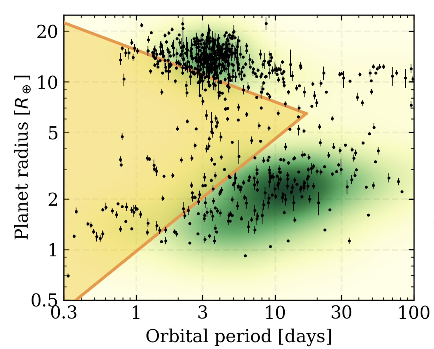
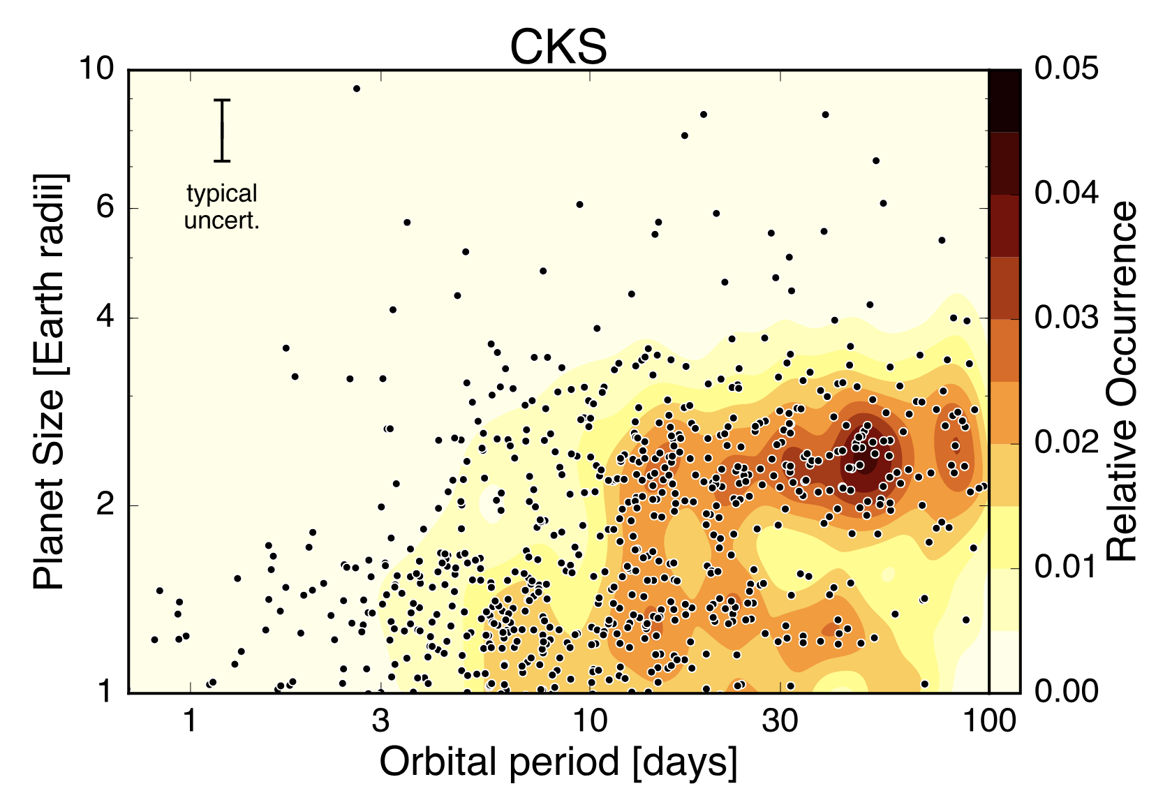
Figure 1: Left panel: the Neptunian desert in the observed exoplanet demographics (in the parameter space of planet size and orbital period). The yellow-shaded region under the triangular boundary shows the Neptunian desert area. The triangular desert boundary is defined by Mazeh et al (2016). The figure is taken from Cloutier (2024) who modified the original version from Osborn et al (2023). The filled contours show the number density of confirmed exoplanets and black markers show the observed planets from NASA exoplanet archive. Right panel: radius valley observed in the small exoplanets from California-Kepler Survey (CKS) from Fulton et al (2017).

The plan for the review is as follows. In the next section, we explain the physical processes that are responsible for atmospheric escape. The observational aspects of atmospheric escape for different exoplanets (e.g., gas giants, rocky exoplanets) are discussed in section 3. In section 4, I explain various theoretical models that incorporate different atmospheric escape processes and their results including comparison with the observations. The evolution of the planetary atmosphere and the role of stellar environments in the evolution process is discussed in section 5. Finally, I will summarise the review with future outlooks in section 6.

2 Physical processes of atmospheric escape

In this section, I will review all the processes that have been suggested in the literature for atmospheric escape. I aim to explain the main parameters for each escape process and I will discuss whether it is possible to relate each escape process with some observable. As we discussed before, the atmospheric escape processes are largely divided into two main procedures based on their driving mechanisms: thermal escape and non-thermal escape. We discuss below both of the escape mechanisms in detail.

2.1 Thermal escape

Thermal escape is one of the important processes which is responsible for atmospheric loss from exoplanets. The X-ray and extreme ultraviolet radiation (hence XUV) from the host star mostly control the thermal escape from the exoplanets (García Muñoz, 2007). Depending on the intensity of the radiation, thermal escape has two limits - Jeans escape and hydrodynamics escape.

2.1.1 Jeans escape

If the upper atmosphere of the exoplanets is in local thermodynamic equilibrium or close to it, then their distribution function can be approximated by a Maxwellian distribution, which is given below following Gronoff et al (2020):

$$f(\vec{x},\vec{v})=N\left(\frac{m}{2\pi kT}\right)^{3/2}e^{-\frac{mv^{2}}{2kT}}=N\left(\frac{1}{u_{i}\sqrt{\pi}}\right)^{3}e^{-v^{2}/u_{i}^{2}},$$ (1)

where $\vec{v}$ and m are the average velocity and mean mass of atmospheric particles respectively. T is the temperature of the upper atmosphere and $u_{i}$ = $\sqrt{\frac{2kT}{m_{i}}}$ is the velocity of the individual species. If some of the atmospheric species achieve escape velocity $v_{\rm esc}=\sqrt{\frac{2GM}{r}}$, they escape to space. The particle in this type of escape process moves from the collisional regime to the collisionless regime as shown in figure 2(a). The boundary between these two regimes is called exobase where the mean free path of the escaping species is greater than the scale height. Also, it has been inherently assumed that the escaping species would not impact another molecule while escaping.

An important parameter that is introduced to account for the Jeans escape in planetary atmospheres is called Jeans parameter $\lambda_{esc}$. This parameter is defined as the ratio of gravitational energy to the thermal energy-

$$\lambda_{esc}=\frac{GMm_{i}/r}{kT}=\frac{v_{\rm esc}^{2}}{u_{i}^{2}}$$ (2)

For the $\lambda_{esc}>2.5$, the Jeans escape becomes significant. To calculate, the escape flux of escaping atmospheric particles, we approximate the distribution to be Maxwellian at the exobase and integrate the vertical flux, $u_{i}cos\theta\times f_{i}$ over the planet surface (Gronoff et al, 2020), which gives

$$\phi_{i}(\rm escape)=N_{i}\left(\frac{u_{i}}{2\sqrt{\pi}}\right)(1+\lambda_{esc})e^{-\lambda_{esc}}.$$ (3)

However, as the particles that are faster than the escape velocity already left to space, a non-Maxwellian correction must be applied to consider this depletion of the high energy tail of Maxwellian distribution (Chamberlain and Smith, 1971). To capture the Jeans escape realistically one should solve the Boltzmann equation and there were few efforts to solve this using the Direct Monte Carlo simulation method (Volkov et al, 2011).

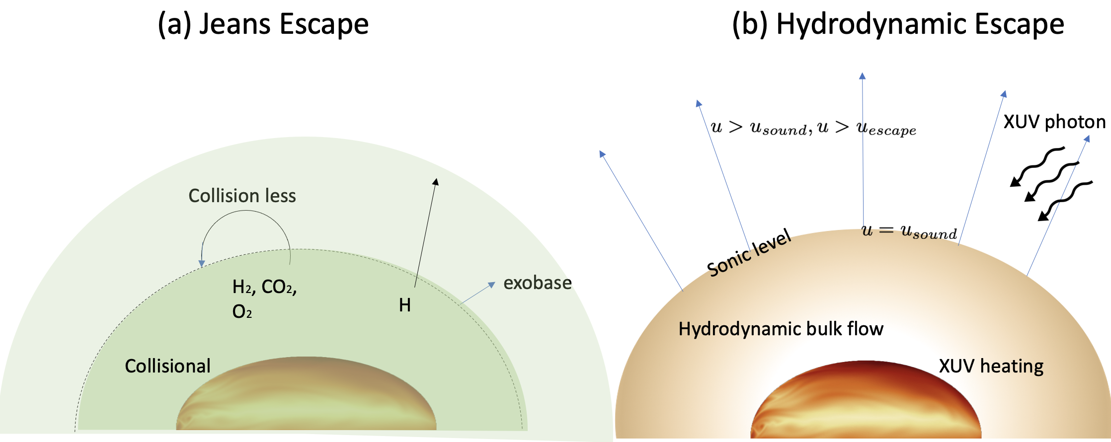
Figure 2: Schematic diagram of different types of thermal escape. (a) Jeans escape - atmospheric particles escape from a collisional atmosphere to a collisionless regime. (b) Hydrodynamic escape - Collsional outflow due to stellar radiation heating mostly by X-ray and extreme ultraviolet part of the spectra

2.1.2 Hydrodynamic escape

Hydrodynamic escape is a more dramatic version of Jeans’ escape. If the internal energy of the individual particle of the atmosphere approaches the kinetic energy for escape, then the gas will escape as a continuous fluid. In hydrodynamic escape, the bulk of the collisional atmosphere leaves the planet as planetary outflow which is similar to the Parker wind (see figure 2(b)). This type of atmospheric escape happens when the planet is irradiated with intense stellar radiation. The fundamental distinction between the Jeans escape and hydrodynamic escape is that atmospheric particles leave from the collisional domain to the collisionless domain by particle to particle but for hydrodynamic escape, the whole bulk collisional atmosphere leaves the planet as hydrodynamic fluid flow.

The hydrodynamic escape is modeled using the same equation as the thermal Parker wind with an added external heating source. In Parker wind, the flow gets accelerated by gas pressure from subsonic to supersonic via a critical sonic point but in hydrodynamic escape, the external heating from stellar UV irradiation adds a major source of fluid acceleration. The hydrodynamic outflow originates from the sub-stellar point on the planet and mass-loss occurs in the form of a steady transonic wind. The basic equations that govern the hydrodynamic escape are the mass continuity, momentum conservation, and energy equation in the steady state:

$$\frac{\partial}{\partial r}(r^{2}\rho u)=0$$ (4)

$$u\frac{\partial u}{\partial r}=-\frac{1}{\rho}\frac{\partial P_{T}}{\partial r}-\frac{GM_{\rm pl}}{r^{2}}+\frac{3GM_{\star}r}{a^{3}}$$ (5)

$$\rho u\frac{\partial}{\partial r}\left[\frac{k_{B}T}{(\gamma-1)m}\right]=\frac{k_{B}T}{m}u\frac{\partial\rho}{\partial r}+\cal{H}-\cal{C},$$ (6)

where the notations are as usual. $\cal{H}$ and $\cal{C}$ represent the heating and cooling rates of the atmosphere, which are modeled separately. In the momentum equation, in addition to gravity force, a tidal gravity term is added in the last part. The tidal gravity term includes a summation of centrifugal force and differential stellar gravity along the ray joining the planet to the star. In the energy equation, the heating due to stellar radiation is implemented. For simplicity, it is a general practice to assume the stellar XUV flux is concentrated at one photon energy $h\nu_{0}$ = 20 eV and calculate the corresponding heating rate as $\Gamma=\epsilon F_{\rm xuv}e^{-\tau}\sigma_{\nu_{0}}n_{0}$ (García Muñoz, 2007; Murray-Clay et al, 2009; Allan and Vidotto, 2019). In this calculation, $n_{0}$ is the number density of neutral H atoms, $\epsilon=(h\nu_{0}-13.6eV)/h\nu_{0}$ is the efficiency representing the fraction of photon energy deposited as heat, and $\tau$ is the optical depth. Note that Kubyshkina et al (2020) and their group assume that the X-ray energy of stellar spectra is concentrated on one wavelength and extreme ultraviolet is distributed over another wavelength. Hazra et al (2020) implemented the heating term using full spectral energy distribution of XUV and concluded that their non-monochromatic approximation gives very similar outcomes as the monochromatic approximation, if an appropriate mean energy (i.e., the XUV radiation is only concentrated on a single wavelength of photon energy 20 eV) is adopted . For the gas giants’ atmosphere, different treatments of the stellar radiation do not affect the mass loss rate significantly (Hazra et al, 2020) but for the small rocky exoplanets, full spectral energy distribution is necessary because they consist of many atmospheric species and photochemical reaction becomes important in all wavelength ranges (Johnstone et al, 2018; Johnstone, 2020).

Radiation cooling plays an important role in the cooling term $\cal{C}$ of equation 6. For the gas giant atmosphere, the main contribution comes from Ly-$\alpha$ radiation. However, the $H^{+}_{3}$ cooling (Yelle, 2004; Koskinen et al, 2007) and metal cooling (Huang et al, 2023) are also important, even they become dominant in some regions of the upper atmosphere. For the rocky exoplanets, the infrared cooling by CO₂, H₂O, NO and O becomes important (Johnstone et al, 2018). Based on the heating and cooling of the atmosphere, and production and losses of neutral hydrogen, the three hydrodynamic regimes (e.g., Murray-Clay et al, 2009; Bear and Soker, 2011; Salz et al, 2016) have been distinguished - (1) Radiation/Recombination-limited regime, (2) Photon-limited regime and (3) Energy-limited regime. If we concentrate on the production of neutral escaping hydrogen species, then the steady-state continuity equation of neutral hydrogen can be written as following Lampón et al (2021):

$$-u\frac{\partial f_{\rm H^{0}}}{\partial r}+f_{\rm H^{+}}n_{\rm H^{+}}\alpha_{\rm H}-f_{\rm H^{0}}J_{\rm H}=0,$$ (7)

where $u$ is the bulk radial velocity, $f_{\rm H^{0}}$ and $f_{\rm H^{+}}$ are the mole fraction of neutral hydrogen and ionized hydrogen respectively. $n_{\rm H{{}^{+}}}$ is the density of ionised hydrogen; $\alpha_{\rm H}$ and $J_{\rm H}$ recombination and photo-ionisation rates respectively. Based on the production of $f_{\rm H^{0}}$, we can define the advection rate as $P_{\rm adv}=-u\frac{\partial f_{\rm H^{0}}}{\partial r}$ and recombination production rate as $P_{\rm rec}=f_{\rm H^{+}}n_{H^{+}}\alpha_{\rm H}$. We also need to define another important parameter called Ionization Front (IF) - the region of partial ionization where (1- $f_{\rm H^{0}})\geq 0.95$.

Based on the parameters, $P_{\rm rec}$, $P_{\rm adv}$, and IF, the three regimes are classified. In the Radiation/Recombination-limited regime, $P_{\rm rec}/P_{\rm adv}>>1$ that means advection is negligible and the gas is almost in radiation-recombination equilibrium. The IF region in this case is very narrow compared with the scale of the flow. Heating efficiency-wise, the incident stellar radiation gets significantly reduced by the radiative cooling, and heating efficiency in this case is much less than 0.1. For the Photon-limited regime, the photo-ionization rate is much faster than the recombination rate and the recombination rate is negligible in the upper atmosphere. Hence $P_{\rm rec}/P_{\rm adv}<<1$. In this case, the IF region extends the whole upper atmosphere of the planet. The energy-limited escape is a scenario between the Radiation/Recombination regime and the Photon-limited regime, where advection and recombination rate - none of them are negligible in the upper atmosphere. In this case, the IF is wide but not as wide that it encompasses the entire flow as the photon-limited regime. For the photon-limited and energy-limited regime, the stellar heating is higher as radiative cooling is moderate or negligible, and the heating efficiency is about 0.1.-0.2. All the heating efficiency mentioned here holds true considering the planetary upper atmosphere is hydrogen-dominated. Proper measurements of these hydrodynamic escape regimes are important because different regimes give different mass-loss rates and constraining them would be invaluable for the long-term evolution of the planetary atmosphere.

2.2 Non-thermal escape

Non-thermal escape from exoplanets involves processes in which the velocity of the escaping particles is not related to the temperature of exobase (Tian, 2015; Gronoff et al, 2020). Non-thermal processes mostly involve the ions and their escape in the presence of electric and magnetic fields. Most of the time, stellar radiation or charge exchange from the solar wind/coronal mass ejections ionizes the neutral constituents of the atmospheres, which further reacts with other neutrals and electrons giving rise to the photochemical escape. Also, the ionized particles can be dragged out of the planet by the solar wind magnetic field. Depending upon the mass, atmospheric composition, magnetic field of the planet, and orbital distance of the planet from its host star, the non-thermal loss varies. For small rocky exoplanets, photochemical loss becomes important because the exothermic chemical reaction from ionized particles in the atmosphere could provide enough kinetic energy for the escape of the neutral particles in the atmosphere.

The interaction of the upper atmosphere and ionosphere with the solar wind and coronal mass ejections from the host star also significantly contributes to atmospheric mass loss. Neutral atoms in the upper atmosphere get ionized by stellar XUV radiation, charge exchange, and electron impact and are swept away by the magnetic field of solar wind plasma. Pick-up ions, sputtering, and charge exchange contribute significantly to the ion escape to space. Ion escape is one of the major sources of mass loss from the solar-system planets and is also believed to be a great contributor to the mass loss from exoplanets.

For magnetized planets such as Earth, the pick-up process is less efficient because in that case, the solar and interplanetary electric and magnetic fields remain far from the planet. Ions in the upper atmosphere get trapped in the magnetosphere of the planet and do not necessarily escape the planet. There are two ways the ions could escape in this scenario. For planets with dipolar magnetosphere, the ions can escape to space by the drag of polar outflow. Also, these trapped ions in the planet’s magnetic field can eventually escape by charge exchange from the solar/stellar wind plasma. Sputtering is another non-thermal process that is widely believed to be very dominant for escape processes in early Mars and Venus (Luhmann et al, 1992; Persson et al, 2021) and also very relevant for exoplanet atmosphere (Gu et al, 2023).

3 Observation of atmospheric escape from exoplanets

Transmission spectroscopy has been used as a very reliable way of measuring atmospheric escape from exoplanets. Exoplanets that are transiting in front of their parent stars provide detailed access to their atmosphere. While exoplanets are in transit, it is possible to separate the planet’s signal from that of the parent star allowing us measurement of atmospheric properties of those planets. A transit event (figure 3) allows us to three fundamental measurements for exoplanet characterizations: (1) Transmission spectra - allow us to measure the composition of the atmosphere from the atmospheric absorption features, (2) emission spectra - during the secondary eclipse, the day side average emission of the planet allows us to estimate average temperature of the planet and (3) the phase curve– by measuring a planet throughout a full orbit, an estimate of the day-to-night temperature contrast can be obtained, which allow us to infer about atmospheric recirculation. As we are interested in atmospheric escape, we focused on the transmission spectra only.

During a transit event, the planet blocks out some of the stellar light, which we can measure by time-series photometry (see figure 3). By measuring accurately how much light is being blocked by transiting exoplanets, the fundamental properties of those exoplanets such as mass and radius can be determined. The computed fractional flux deficit measured from the stellar light curve (see the black curve in the bottom panel of figure 3), which is proportional to the projected area between the planet and star, gives the planet-to-star radius ratio. Also, the detailed spectroscopic information of this absorbed light gives us the atmospheric properties of exoplanets. The atmospheric atoms and molecules of planets will absorb and scatter lights at their characteristic wavelengths making the atmosphere opaque on those wavelengths at higher altitudes as shown in the bottom panel of figure-3 by the red solid line. Hence measuring the transit spectra in different wavelengths, in principle, we probe different atmospheric compositions in higher altitudes. This is the basic idea of transmission spectroscopy and using this many atmospheric species that are leaving the atmosphere of exoplanets have been detected.

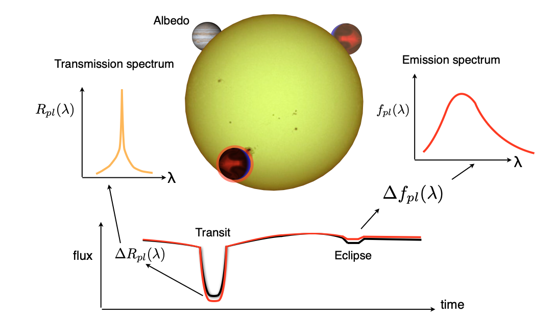
Figure 3: A detailed picture of transit spectroscopy when a planet is transiting its host star. Taken from Sing (2018). The top middle panel shows the scenario of the planet during transit and secondary eclipse. A transmission spectrum as a function of wavelength is shown in the top left. Thermal emission spectrum as a function of wavelength in infrared is measured by the change in the eclipse depth shown in the top right. The transit and eclipse events are shown in the bottom panel. The albedo (fraction of the reflected light from the planet) is measured by observing the secondary eclipse at optical wavelength.

As the light elements in the exoplanetary atmosphere such as hydrogen and helium are more susceptible to getting lost in space, the first efforts were rightly put toward the detection of hydrogen in exoplanet atmospheres. The most successful observational probe to establish atmospheric escape comes from the observation of Ly-$\alpha$ transmission from various hot Jupiters and warm Neptunes. Vidal-Madjar et al (2003) first found evidence of atomic neutral hydrogen absorption in stellar Ly-$\alpha$ by measuring three transits of HD209458b using the Space Telescope Imaging Spectrograph on board HST. The large absorption $15.0\pm 4$ % of stellar Ly-$\alpha$ indicates a large extended envelope of neutral hydrogen, which is beyond the gravitational influence of the planet and hence escaping. This is the first confirmation of neutral hydrogen escaping from the planet HD209458b. Subsequently, many other observations also confirmed the escaping of neutral hydrogen from other exoplanets. For example, Lecavelier Des Etangs et al (2010); Lecavelier des Etangs et al (2012) found escaping neutral hydrogen in the hot Jupiter HD 189733 b. The warm Neptune GJ436b is a very interesting candidate where an extended tail of escaping neutral hydrogen is observed (Kulow et al, 2014; Ehrenreich et al, 2015; Lavie et al, 2017). In the figure 4, a depiction of the observed extended tail of escaping neutral hydrogen atmosphere is shown (obtained from Bourrier et al (2016) ). This planet shows the absorption of stellar Ly-$\alpha$ of $56.3\pm 3.5$ %, which shows, so far, maximum absorption of neutral hydrogen representing a huge amount of atmosphere is leaving the planet (Ehrenreich et al, 2015). Bourrier et al (2018) also reported neutral hydrogen escaping from another warm Neptune GJ3470b with maximum absorption of $35\pm 7$ %. There are some limited observations of escaping hydrogen using H-$\alpha$ line also (Jensen et al (2012); Barnes et al (2016); Cauley et al (2017), Yan and Henning (2018); Czesla et al (2022); Bello-Arufe et al (2023)).

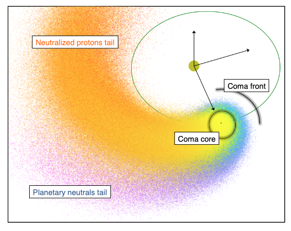
Figure 4: A schematic diagram showing the escape of neutral hydrogen from the warm Neptune GJ436b. It shows the planet has an extended tail made of neutral hydrogen and protons. Taken from Bourrier et al (2016)

The stellar Ly-$\alpha$ absorption by planetary atmosphere gives a tremendous opportunity to probe atmospheric escape from the exoplanets, however, note that due to Geo-coronal emission and ISM absorption some part of the Ly-$\alpha$ in the velocity range -50 to +50 km s^-1 is not directly observable. As a result, they can not be used to probe the launching region of the planetary outflow as the typical velocity of the gas going through the atmospheric escape is $\leq 20$ km s^-1. The H-$\alpha$ absorption certainly can probe this regime but very limited detection is available due to stellar contamination in the H-$\alpha$ signal. The helium transit line 10830 Å plays an important role in probing this inaccessible region of planetary outflow. A major advantage of obtaining helium spectra is that we can observe them from ground-based telescopes. Recently, there have been significant efforts for the successful detection of He lines from exoplanets from ground based-faciliteis (CARMENES, SPIRou, GIANO, Keck/NIRSPEC) as well as Wide Field Camera 3 on board HST (e.g., Allart et al, 2018; Oklopčić and Hirata, 2018; Spake et al, 2018; Zhang et al, 2022a; Allart et al, 2023; Masson et al, 2024; Krishnamurthy and Cowan, 2024; McCreery et al, 2025). Helium detections have been reported in numerous exoplanet targets such as HAT-P-11b (Allart et al, 2018), WASP-107b (Spake et al, 2018), WASP-69b (Nortmann et al, 2018), HD209458b (Alonso-Floriano et al, 2019), HD189733b (Salz et al, 2018) and TOI-1807b (Masson et al, 2024).

Recently, there have been global surveys (e.g., Allart et al, 2023; Guilluy et al, 2023; McCreery et al, 2025) of detecting helium from exoplanets using ground-based facilities. To find a definite correlation between mass-loss rate and presence of helium, these homogeneius large-scale analyses is needed. Allart et al (2023) searched for helium in 11 gas giants with SPIRou but they could not conclude a definite correlation between mass-loss rate and presence of helium, and argued that it still requires larger-scale analysis of the helium triplet. McCreery et al (2025) analyzed archival helium exoplanet transmission spectra that are detected and publicly available, and concluded that the mass-loss rate follows the energy-limited approximation.

In addition to light elements, some other elements including some metals were also found to be escaping from exoplanets (e.g., Vidal-Madjar et al, 2004; Fossati et al, 2010; Cubillos et al, 2020; Ben-Jaffel et al, 2022). Vidal-Madjar et al (2004) from HST measurement detected oxygen(O I) and carbon (C II) in the upper atmosphere of exoplanets that are going through hydrodynamic escape. Recently, ionized iron and ionized magnesium have been observed in hot Jupiters, which must be dragged into the upper atmosphere by the escaping hydrogen and helium (e.g., Sing et al, 2019; Cubillos et al, 2020).

Most of the observational studies of atmospheric escape focused on gaseous exoplanets (e.g., hot Jupiters, warm Neptunes, hot Saturns) because the gaseous exoplanets go through rapid hydrodynamic escape and they are good candidates for atmospheric studies. However, to the best of our knowledge recently there have been no studies that have directly observed atmospheric escape of small rocky exoplanets from observations. Recently dos Santos et al (2019) discussed the possibility of detection of the excess Ly-$\alpha$ absorption signal by hydrogen exosphere around Earth-like planets but we need next-generation spectrographs such as LUVOIR/LUMOS (France et al, 2017) to detect it. Also, there is indirect evidence that small rocky exoplanets went through the atmospheric escape in the early evolution times and gave rise to the radius gap (Fulton et al, 2017).

3.1 Is it possible to segregate different regimes of atmospheric escape from observations?

As we mentioned in section 2, the atmospheres of exoplanets go through different types of escape processes, and depending on what kind of process is responsible for their atmosphere to escape, mass-loss rate could be defined. For the solar system planets, there are some studies to understand the transition between Jeans escape and hydrodynamic escape (e.g., Volkov et al, 2011; Erkaev et al, 2015). For the exoplanets, the transition between Jeans escape and hydrodynamic escape has not been studied at all from observations. However, Lampón et al (2021) successfully distinguished the three hydrodynamic escape regimes that theoretical models predicted (see section 2.1.2) by observing transmission helium triplet lines and Ly-$\alpha$ in gaseous exoplanets.

The high-velocity neutrals ($\simeq$ 200 km s^-1) observed in Ly-$\alpha$ during the transit event from gaseous exoplanets (e.g., Lecavelier des Etangs et al, 2012; Ehrenreich et al, 2015) are signature of escape which are most likely driven by stellar wind/coronal mass ejection interaction (Carolan et al, 2020; Hazra et al, 2022). Since the XUV-driven thermal escape can not accelerate neutral particles typically beyond 20-30 km s^-1 (Murray-Clay et al, 2009; Salz et al, 2016; Kubyshkina et al, 2018b; Allan and Vidotto, 2019; Hazra et al, 2020; Schreyer et al, 2024; Rosener et al, 2025), high-velocity neutrals are due to non-thermal escape from the planet and can be differentiated from low-velocity thermal escape ($\leq$ (20 - 30) km s^-1).

4 Numerical models to understand atmospheric escape

Exoplanet research is a relatively new field only 2 decades old. After the first detection of atmospheric escape from the hot Jupiter HD209458b in 2003 (Vidal-Madjar et al, 2003), different groups started to develop theoretical models to understand the atmospheric escape from exoplanets. The early efforts were based on 1D models for both gas giants and rocky terrestrials exoplanets (e.g., Yelle, 2004; Tian et al, 2005; García Muñoz, 2007; Murray-Clay et al, 2009; Guo, 2011; Koskinen et al, 2013; Johnstone et al, 2015; Guo and Ben-Jaffel, 2016; Kubyshkina et al, 2018a; Johnstone et al, 2018; Allan and Vidotto, 2019; Hazra et al, 2020). With time, 1D escape models have been enriched with detailed complicated physics, and still, new things are being added to those models. However, some of the aspects can not be modeled using simple spherically symmetric models. For example, the observed extended tail-like structure (Ehrenreich et al, 2015) of transiting exoplanets can not be modeled using 1D models. The day-night asymmetry, changes in temperature between day and night sides, and the complex magnetospheric structure could only be modeled using 3D models. The 3D models of atmospheric escape have also been started a decade ago and they are now becoming very sophisticated in explaining various observational results of atmospheric escape from gas giants (e.g., Tripathi et al, 2015; Villarreal D’Angelo et al, 2014; Khodachenko et al, 2015; Christie et al, 2016; Carroll-Nellenback et al, 2017; Villarreal D’Angelo et al, 2018; Esquivel et al, 2009; McCann et al, 2019; Carolan et al, 2020; Hazra et al, 2022; MacLeod and Oklopčić, 2022), as well as from terrestrial exoplanets (e.g, Dong et al, 2017; Garcia-Sage et al, 2017; Dong et al, 2018, 2019). In the next few sections, I will discuss 1D models and 3D models for atmospheric escape including their results.

4.1 1D escape models

The first kind of hydrodynamic escape model was developed by Yelle (2004) for the giant planets that are orbiting the host star in very close proximity within 0.01 to 0.1 AU. They solve the usual fluid equations for hydrodynamic escape (see section 2.1.2) with stellar heating, adiabatic cooling, and photochemical reactions. Their model included neutral species H₂, He, and H and ionized species H⁺, H${}^{+}_{2}$, H${}^{+}_{3}$, He⁺, and HeH⁺ and solved the continuity equation and diffusion equation along with momentum, energy equations for the composition of the upper atmosphere of giant planets. The mass-loss rate (escape rate) 10⁸ g s^-1 calculated from their model was 100 times smaller than the mass-loss rate estimation of Vidal-Madjar et al (2003) from Ly-$\alpha$ observation. I shall use mass-loss rate or escape rate interchangeably in this whole review if not otherwise mentioned.

The discrepancy in the mass-loss rate for the giant planets obtained from the model of Yelle (2004) and observations instigated further study on this topic. Tian et al (2005) used updated two-dimensional heat deposition studying hydrodynamic escape of hydrogen-rich atmosphere. They found the atmospheric mass-loss rate of $6\times 10^{10}$ g s^-1, which is in good agreement with the observed value from HD209458b despite the assumption of solar equivalent EUV radiation from the host star. With a sophisticated molecular diffusion model, García Muñoz (2007) was also able to find a mass loss rate comparable to the observation. Murray-Clay et al (2009) have added self-consistent radiative transfer for the stellar EUV heating and radiative cooling and computed the hydrodynamic equations for escape calculation. In addition to the calculation of a mass-loss rate of neutral hydrogen, they calculated the synthetic transit spectra for direct comparison with the observed transit calculation of Ly-$\alpha$ for HD209458b (Vidal-Madjar et al, 2003).

In the left panel of figure 5, I show the theoretically computed synthetic spectra for neutral hydrogen absorption in the Ly-$\alpha$ line from Murray-Clay et al (2009). The plot shows the amount of stellar Ly-$\alpha$ obscured by the planetary atmosphere ($e^{-\tau}$), which is estimated by calculating line-of-sight optical depth integrated up to a maximum altitude of 10R_p, where R_p is the radius of the planet. The horizontal dashed line shows the geometrical visible continuum. Two sets of dotted and dot-dashed lines show the Doppler velocity of escaping material near $\pm 100$ km s^-1. In the right panel, the dashed line and dotted line show the observed out-of-transit and in-transit spectra. The line-core (-42 to +32 km s^-1) is set to zero where interstellar absorption is strong. Using the theoretical absorption (as shown in the left panel of this figure), the in-transit spectrum is overplotted using a solid line. It has been found that the theoretical model of Murray-Clay et al (2009) was not able to explain the observed 15% absorption in the high-velocity neutrals. The model spectra showed a decrement of 3% of stellar flux in the observed in-transit line spectrum. A plausible reason for this less absorption in the high-velocity neutrals is the absence of stellar wind interaction with the planetary outflow, which needs multidimensional modeling (see next section 4.2). Based on the relations between both stellar heating and radiation cooling with mass-loss rate, Murray-Clay et al (2009) found that for the intense XUV flux from the star, the atmospheric escape is radiation/recombination limited, and for low XUV flux, it is energy-limited.

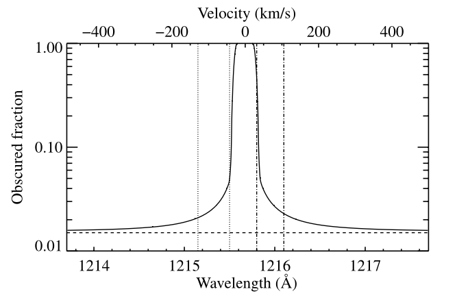
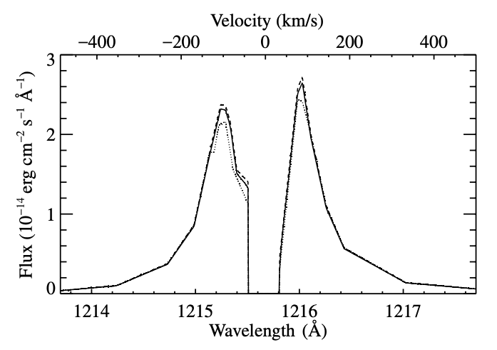
Figure 5: left: Synthetic Ly-$\alpha$ transit spectra computed from the escaping hydrogen atmosphere of HD209458b. All required density, velocity, and temperature for synthetic spectra are computed using the escape model of Murray-Clay et al (2009). Right: Direct comparison of simulated spectra with the observed spectra after correcting for the interstellar absorption. Taken from Murray-Clay et al (2009)

The above models explained so far have assumed the planetary atmosphere is dominated by hydrogen-helium. However,Vidal-Madjar et al (2004) found other species in the atmosphere are escaping too. Koskinen et al (2013) added heavier atoms and ions in their calculation of hydrodynamic escape and discussed the possibility of the presence of heavier neutral and ionized atoms in the upper atmospheres.

One of the major approximations in the Murray-Clay et al (2009) while implementing radiative transfer is the monochromatic approximation - all stellar spectral energy distribution (SED) is concentrated on a single wavelength corresponding to energy of 20 eV. This approximation was reasonable given the difficulty in observing the full SED from the host stars. However, with new techniques and machine learning, it is possible to obtain SED from stars (Sanz-Forcada et al, 2011; Linsky et al, 2014; France et al, 2016, 2020; Behr et al, 2023). Hazra et al (2020) considered a full SED from the host star and studied the effect of full SED on the hydrogen-dominated atmosphere. They assumed a hypothetical hot Jupiter orbiting our present Sun and obtained full solar SED in the XUV regime, which was driving the atmospheric escape. The comparison of physical properties of the atmosphere for both monochromatic approximation and full SED implementation are shown in figure 6. The results for both cases are not very different except for the temperature profile and the ionization fraction. In the right panel of the bottom row, half of the ionization fraction is marked using a red horizontal dashed line. Interestingly, the ionization is stronger for the monochromatic case which will in principle predict less Ly-$\alpha$ absorption due to less neutral hydrogen but can not be probed by observation as the line core of Ly-$\alpha$ is not visible.

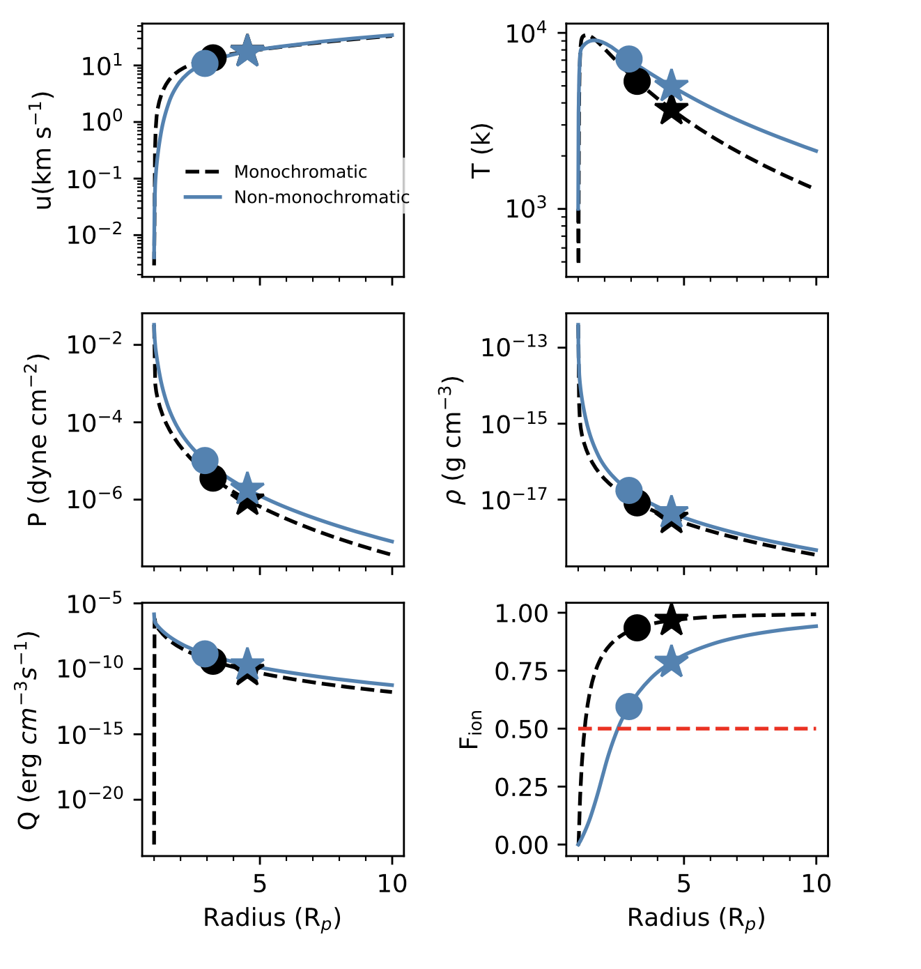
Figure 6: Behaviour of upper atmosphere of a hot Jupiter from the simulation of hydrodynamic escape for monochromatic and non-monochromatic radiative transfer of stellar radiation. The black dashed line and solid blue lines show monochromatic and non-monochromatic cases respectively. The velocity (u) and temperature (T) of the escaping materials are shown on the left and right of the top panel. Similarly, pressure (P) and mass density ($\rho$) are presented in the middle row. The total volumetric heating rate and ionization fraction of hydrogen are given in the left and right of the bottom row, respectively. This figure is adopted from Hazra et al (2020). The filled circles show the sonic point and star markers show the Roche lobe boundary for the star-planet system that they considered.

With the recent discovery of helium as an excellent probe for the escaping atmosphere, there are some efforts (e.g., Dos Santos et al, 2022; Biassoni et al, 2024; Linssen et al, 2024; Rosener et al, 2025) in developing 1D hydrodynamic escape model that interpret helium observations and retrieve the atmospheric mass-loss and temperature of upper atmosphere. Dos Santos et al (2022) developed an open source python code p-winds that couples a purely upper atmosphere H + He Parker wind model with ionization balance, ray tracing and radiative transfer. By fitting p-winds models with observed helium spectra, they are able to estimate mass-loss from the planet but the model results depend on the hydrogen mass fraction. In a similar line, Linssen et al (2024) developed a model called sunbather which couples Cloudy interface for doing photoionsiation and radiative transfer calculation with p-winds. The open source code Pluto has been also used to simulate upper atmosphere by coupling with Cloudy to develop an open source code pyTPCI for simulating outflows and their signature in helium and metal lines (Rosener et al, 2025).

For the small terrestrial exoplanets, the computation of atmospheric escape involves much-complicated photochemistry, heating, and radiative cooling. Johnstone et al (2018) considered heating from the absorption of stellar X-ray, UV, and IR radiation. They also included heating from exothermic chemical reactions, electron heating from collisions with non-thermal photoelectrons, and Joule heating. For the cooling, cooling from infrared emission by several species is included. The thermal conduction and energy exchanges between the neutral, ion, and electron gases are included in their model. Altogether, they considered a chemical network that includes $\sim$ 500 chemical reactions including 56 photoreactions, eddy and molecular diffusion, and advection. This sophisticated model has been validated by studying the thermospheric structure of Earth and Venus. For modeling the upper atmosphere of terrestrial planets and understanding atmospheric escape from them, this type of model will play a significant role.

Most of the 1D models that we discussed above dealt with the hydrodynamic escape from the gas giants and terrestrial exoplanets, as hydrodynamic escape is quite significant for evolution. In addition, most of the observations available from the transit calculation, are for those planets which are very close to the host star. Being in close proximity to the host star, it is expected that planets would go through extreme hydrodynamic mass loss. For solar system planets, the Jeans parameter (see equation 2 in section 2.1.1) is a very good indicator to understand if the planet is going through the Jeans escape or hydrodynamic escape (e.g., Volkov et al, 2011). Generally, if a Jeans parameter is larger than $\sim$ 2-3.6, a transition from hydrodynamic escape to Jeans escape occurs. There were not many studies on exoplanets to understand which type of escapes are going on exoplanets until recently Guo (2024) analyzed a large sample of approximately 2700 planets orbiting G and M-type stars, which are receiving XUV flux and under the influence of their host stars. By defining a new Jeans parameter ($\lambda^{*}_{\rm esc}$) which takes into account the effect of tidal force (tidal force is not very important for solar system planets as they are far from the Sun), a new limit on it is set for the transition of hydrodynamic escape to Jeans escape. They reported that, unlike solar system planets, Jeans escape does not occur for close-in exoplanets if the $\lambda^{*}_{\rm esc}$ is larger than 3. Even XUV-driven hydrodynamic escape can happen if $\lambda^{*}_{\rm esc}$ is more than 100.

4.2 Multi-dimensional escape models

The 1D escape models were successful in reproducing many features of atmospheric escape qualitatively including mass loss rates but the details of atmospheric escape such as day-night asymmetry, comet-like structure, and presence of high-velocity neutrals ($\geq$ 100 km s^-1) in the upper atmosphere were not possible to capture in 1D. The first kind of multidimensional atmospheric escape simulation was started by Stone and Proga (2009) in two dimensions. This model used a simplified treatment of radiative transfer and thermodynamics. The multi-dimensionality of the model produces significantly different results than spherically symmetric models with the same parameters. The mass-loss rate was reduced 4 times in these models than in spherical wind and the sonic point is close to the planetary surface.

The 3D simulations of the atmospheric escape process with a sophisticated treatment of radiative transfer and detailed microphysics have been performed by many groups till now (e.g., Tripathi et al, 2015; Villarreal D’Angelo et al, 2014; Khodachenko et al, 2015; Christie et al, 2016; Carroll-Nellenback et al, 2017; Dong et al, 2018; McCann et al, 2019; Carolan et al, 2020; Hazra et al, 2022). Here we mention a few. Tripathi et al (2015); McCann et al (2019) performed atmospheric escape simulations using open-source Athena code and Carroll-Nellenback et al (2017); Debrecht et al (2020) used Astrobear code. Hazra et al (2022) developed a 3D radiation-hydrodynamic escape model based on open source BATS-R-US code. They simulated the upper atmosphere of hot Jupiter HD189733b based on self-consistent radiative transfer of stellar heating and radiative cooling. They solve the hydrodynamic equations in 3D cartesian grids that include adaptive mesh refinement as given below:

$$\frac{\partial{\rho}}{\partial{t}}+\nabla\cdot\rho{\vec{u}}=0,$$ (8)

$$\frac{\partial(\rho\vec{u})}{\partial t}+\nabla\cdot[\rho\vec{u}\vec{u}+P_{T}I]=\rho\bigg{(}\vec{g}-\frac{GM_{*}}{(r-a)^{2}}\hat{R}-\vec{\Omega}\times(\vec{\Omega}\times\vec{R})-2(\vec{\Omega}\times\vec{u})\bigg{)},$$ (9)

$$\frac{\partial}{\partial t}\left(\frac{\rho u^{2}}{2}+\frac{P_{T}}{\gamma-1}\right)+\nabla\cdot[\vec{u}(\frac{\rho u^{2}}{2}+\frac{\gamma P_{T}}{\gamma-1})]=\rho\bigg{(}\vec{g}-\frac{GM_{*}}{(r-a)^{2}}\hat{R}-\vec{\Omega}\times(\vec{\Omega}\times\vec{R})\bigg{)}\cdot\vec{u}~$$

$$+{\cal H}-{\cal C}~~.~~~~~~$$ (10)

All notation is usual and details are given in Hazra et al (2022) and we are not repeating here. However, it is worth mentioning some comments on the numerical resolution. Any numerical simulation should be able to resolve the scale height of the atmosphere to capture the underlying atmospheric variations. For example, the hydrostatic pressure scale height $H$= $kT/(m_{H}g)$ for a typical hot jupiter ($\sim 0.7M_{J}$) = 0.1R_p (Murray-Clay et al, 2009). Hence the numerical resolution in the simulations should be higher than 0.1R_p. Usually, the computational volume around the planet is taken much larger than the planetary environment to minimize the boundary effect. For HD189733b, the Cartesian simulation box considered by Hazra et al (2022) has a rectangular grid with x = [-20, +40]R_p , y = [-40, +40]R_p , and z = [-32,+32]R_p. However, for HAT-P-11b, as the magnetotail is expected to be longer from the condition of stellar wind, a larger computational domain has been used (for details see Ben-Jaffel et al, 2022). The inner boundary for atmospheric escape simulation are fixed at the distance where the UV photons are absorbed (optical depth $>>1$). This is close to the surface of the planet (approximately at a height of 1.1R_p) with atmospheric pressure $\sim 1$ nanobar at the base of the wind. The visible radiation from the star is absorbed at pressure closer to 1 bar at the surface and it takes about 0.1R_p for atmospheric pressure to be reduced from 1 bar to 1 nanobar. In this lower atmosphere (higher pressure zone), we need to generally employ Global Circulation Models to understand the behaviour of the atmosphere. The stellar heating using radiative transfer is implemented in the heating term ${\cal H}$ in the equation 4.2. In this simulation, Coriolis force and centrifugal forces are also included. The atmospheric properties of the planet due to stellar heating are shown in the figure 7. The total density, neutral hydrogen density, temperature, and total velocity of outflowing materials are shown in the four panels (a), (b), (c) and (d) of figure 7 respectively. The 3D model shows morphologically different results than 1D models as expected. The atmosphere of the planet moves in a clockwise direction due to the Coriolis force. The velocity streamlines by black contours (panel (a) of figure 7) show this clockwise movement of the outflowing material clearly. One interesting thing to notice in this atmospheric profile is that total density does not show significant day-night asymmetry as is expected from the stellar heating. However, the neutral density shown in panel (b) has a distinct shadow on the night side of the planet due to no ionization of planetary material. The interplay between tidal force and Coriolis force on the planetary material in different directions creates shocks which are clear from the high-temperature regions in panel (c). In panel (d), the total velocity with the sonic surface is shown. Because of the competition among tidal force, Coriolis force, XUV heating, and gravitational force, the sonic surface varies from the day side to the pole to the night side. This shows the importance of multidimension in simulating the planetary outflow as planetary outflow originates at different distances around the planet.

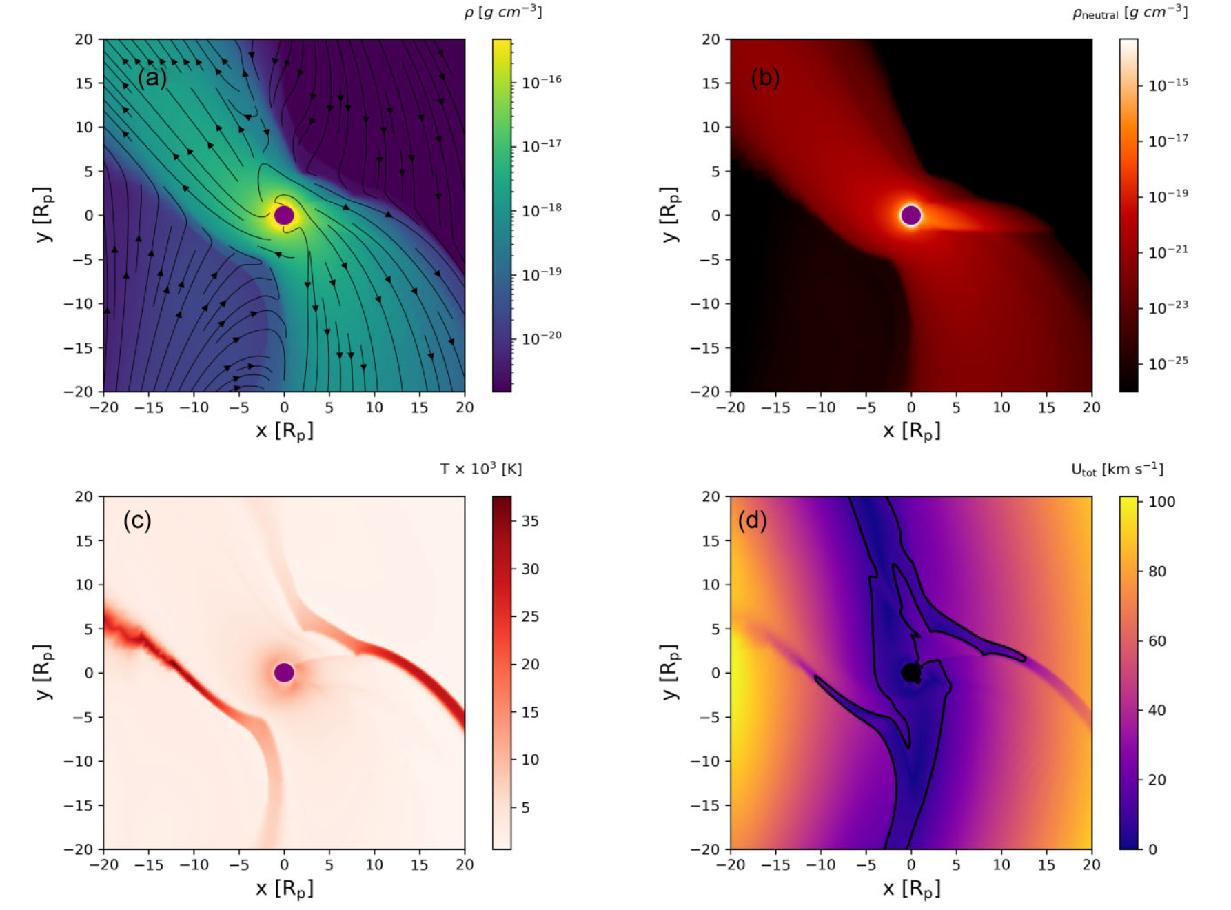
Figure 7: (a)Total density (neutral + ions + electrons) of outflowing materials around the planet. Velocity streamlines are shown in black contours. (b) The neutral hydrogen profile, (c)The temperature distribution, and (d) The total velocity of the outflowing materials including the sonic surface. The planet is in the center of the grid shown using the purple circle. All plots are in the orbital plane. In these all simulations, the host star is kept outside of the simulation domain at the negative axis. Taken from Hazra et al (2022)

The estimated mass-loss rates from the 3D atmospheric escape models (Tripathi et al, 2015; Carroll-Nellenback et al, 2017; McCann et al, 2019) are comparable with observed values (Vidal-Madjar et al, 2003; Lecavelier Des Etangs et al, 2010; Lecavelier des Etangs et al, 2012; Bourrier et al, 2016). For the planet HD189733b, the estimated mass-loss rate from 3D model of Hazra et al (2022) is $6\times 10^{10}$ g s^-1. This value is comparable with several existing models (Guo, 2011; Guo and Ben-Jaffel, 2016; Salz et al, 2016) and observations (Lecavelier des Etangs et al, 2012).

4.2.1 Interaction of stellar wind with planetary upper atmosphere and its importance on atmospheric escape

The hydrodynamic outflow that originates from the planet due to incident stellar XUV radiation interacts further with the plasma environment of the host star. The interaction between stellar wind and planetary outflow due to atmospheric escape shapes up the upper atmosphere of the planets. Vidotto and Cleary (2020) studied the effect of stellar wind on the atmosphere of close-in exoplanets in detail. The competition between stellar wind ram pressure at the orbital distance of the planet and the ram pressure of the exoplanetary outflow at the sonic point decides whether the atmospheric mass loss from the planet will be affected. In figure 8, the scenario is explained. If the stellar wind ram pressure at the orbital distance is stronger than the ram pressure of the planetary outflow at the sonic point, then the planetary outflow gets confined from the supersonic outflow to the subsonic breeze changing the escape rate. This situation is shown in the right panel of figure 8. If the situation is another way i.e, the ram pressure of planetary outflow at sonic pint is stronger than the stellar wind ram pressure, planetary outflow remains unconfined and escape rate does not get affected (see the left panel of figure 8). This is a general consensus about the interaction of stellar wind and its impact on the planetary atmosphere. However, this is based on 1D calculation and purely hydrodynamic interaction between stellar wind and planetary outflow.

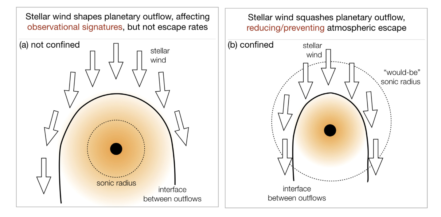
Figure 8: Schematic diagram of confinement of planetary outflow by stellar wind. Left panel: Not confined - the case where stellar wind ram pressure is weaker than the ram pressure of planetary outflow. Right panel: Confined- the case where stellar wind ram pressure is stronger than the ram pressure of planetary outflow. Figure is taken from Vidotto and Cleary (2020)

Some 3D escape models explore the stellar wind interaction with the planetary outflow (e.g., Carroll-Nellenback et al, 2017; McCann et al, 2019; Carolan et al, 2020, 2021b; Wang and Dai, 2021a; MacLeod and Oklopčić, 2022; Hazra et al, 2022; Mitani et al, 2022). In a 3D simulation, McCann et al (2019) found that stellar wind indeed can confine the atmospheric escape from the planetary atmosphere if the stellar wind is sufficiently strong. In figure 9, we show a set of simulations from their paper, which depicts the interaction of stellar wind of three different strengths with planetary outflow that has a constant escape rate for three stellar wind cases. The upper panel shows the orbital plane (z = 0) and the lower panel shows vertical slices perpendicular to the star-planet axis (y = 0). As we expected, the weaker stellar wind in column 1 ((a) and (d)) could not confine the planetary outflow and did not affect the mass loss rate. The intermediate stellar wind could partially confine the planetary outflow (see second column, (b) and (e)). Finally, the strong stellar wind can confine the planetary outflow reducing it to a breeze (column 3, (c) and (f)) of figure 9. The stronger stellar wind ram pressure can suppress the whole day-side outflow and shape the atmosphere of the planet into a comet-like structure, which has been observed already (Ehrenreich et al, 2015; Bourrier et al, 2016). A similar conclusion was also drawn by Carolan et al (2020, 2021b). These results are generally applicable to the hot and warm gaseous planets.

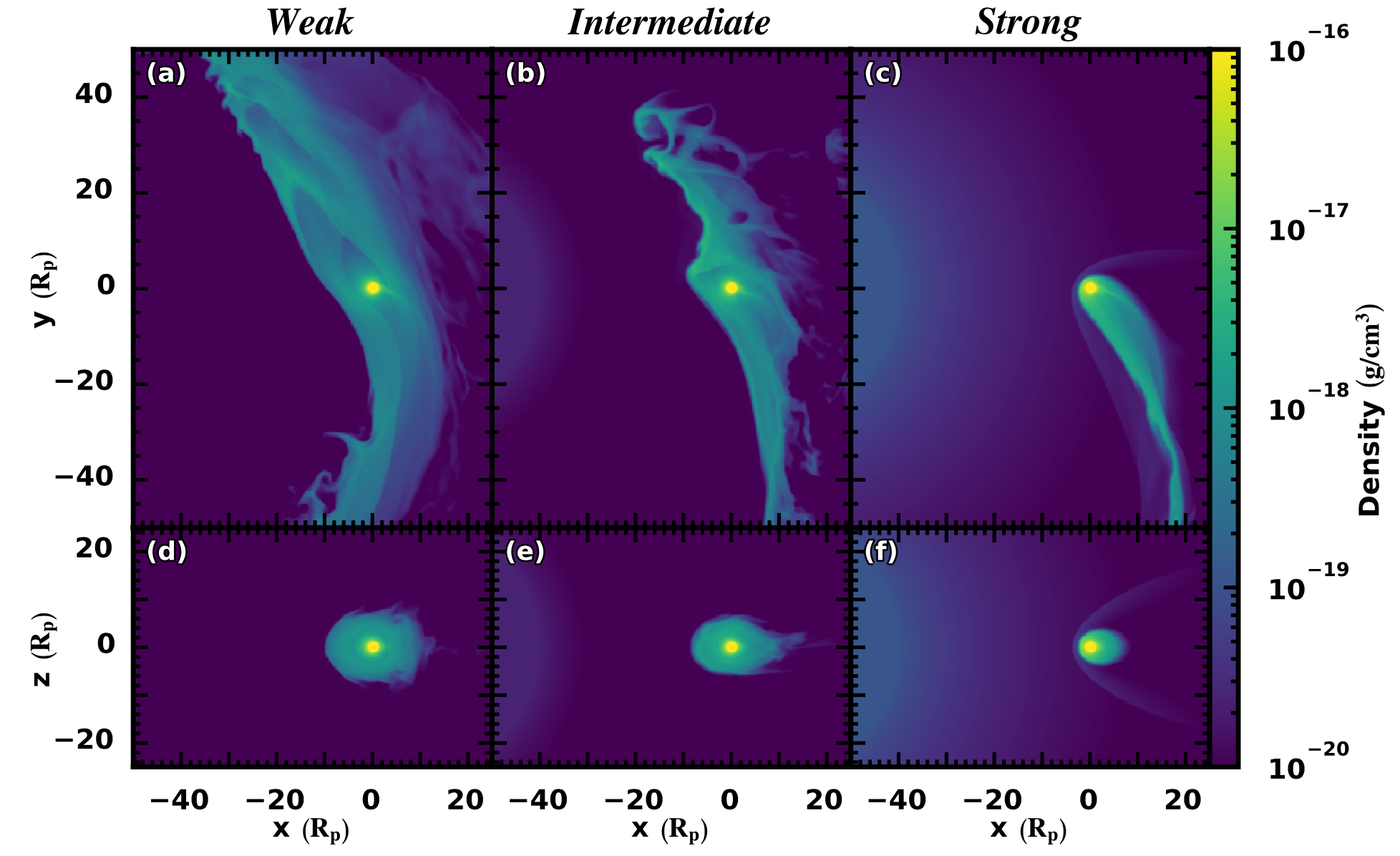
Figure 9: Total density of planetary outflow interacting with the weak (first column), intermediate (second column), and strong (third column) stellar wind . The upper row shows a density pattern in the orbital plane (z=0) and the lower panel shows the same in the polar plane (y =0). The figure is taken from McCann et al (2019)

The interaction of stellar wind with the planetary atmosphere not only changes the mass-loss rate but also changes the transit signature. Most of the simulations (mentioned above) of atmospheric interaction with the stellar wind have been performed so far assuming a hydrogen-rich atmosphere, except a few recent study (Wang and Dai, 2021a, b; Khodachenko et al, 2021; MacLeod and Oklopčić, 2022) that modeled the hydrogen-helium atmosphere. The Ly-$\alpha$ transit signatures have been synthetically generated from these 3D models for different strengths of stellar wind. For details of transit signature calculation from the 3D simulation, please see section 4 of Carolan et al (2021b). Carolan et al (2021b) computed the Ly-$\alpha$ transit signatures for different stellar wind strengths for a hot Jupiter and a warm Neptune, which is shown in figure 10. The stellar wind strength is determined by its mass loss rate. The higher the mass loss, the stronger the wind is. They have performed a series of simulations with varying mass-loss rates of stellar wind from 0 to 100$\dot{M}_{\odot}$. The figure clearly shows that as the stellar wind strength increases, it confines the atmospheric escape but increases the asymmetry in transit absorption spectra. As stellar wind strength increases, transit depths in high-velocity blue wing (integrated transit depth over the velocity range of [-300, -40 km s^-1]) and red wing [+40, +300 km s^-1) decrease for both hot Jupiter and warm Neptune. However, the transit depth in red wing decreases more than the blue wing as with increasing stellar wind strength the day-side outflow gets confined completely. The different colors show the different mass-loss rates of stellar wind.

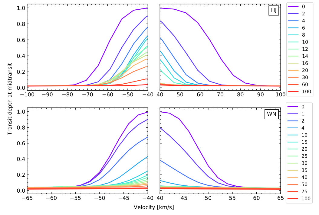
Figure 10: Ly-$\alpha$ transit spectra from atmospheres of a hot Jupiter (top panel) and a warm Neptune (bottom panel) for different strengths of stellar wind from their host stars. The left and right panels show the blue wing [-40 to -300 km s^-1] and red-wing [+40 to +300 km s^-1] parts of the transit spectrum. The different colors represent the variation of stellar mass-loss rate from 0 to 100 $\dot{M}_{\odot}$. The gap in figure from -40 to + 40 km s^-1 is kept as the line center gets contaminated by interstellar absorption and geocoronal emission. This figure is taken from Carolan et al (2021b).

It has been found that the weak stellar wind can not change the mass-loss rate much as the way the stronger stellar wind does, but it changes the transit signatures. Carolan et al (2021b) reported that for stellar wind with mass loss rates $<$ 10$\dot{M}_{\odot}$, the atmospheric escape does not change much but blue wing absorption in Ly-$\alpha$ changes approximately 10% for hot Jupiter to 3% in warm Neptune. MacLeod and Oklopčić (2022) computed the synthetic transit spectra for the metastable helium from their simulation of stellar wind interaction with the planetary atmosphere. They simulated three cases A, B and C with weak, intermediate, and strong stellar wind similar to the cases shown in figure 9. The simulated light curve of excess metastable absorption shows that for the case of weak and intermediate stellar wind (cases A and B in their paper), the helium absorption is not significantly different than the case with no stellar wind. For the strong stellar wind, they found a large absorption in the helium triplet line (see figure-4 of MacLeod and Oklopčić (2022)). This indicates that the stellar wind confines the atmospheric escape with concentrated planetary outflowing materials close to the planet, which increases the optical depth and hence the helium transit depth.

The above argument of the interaction of stellar wind with the planetary atmosphere would be appropriate for most of the hot and warm gaseous planets that are going through hydrodynamic escape. For the small low-mass terrestrial planets with hydrogen-helium envelope, in the early phase of their evolution, the strong hydrodynamic escape in principle would be confined or not, will be decided by the stellar wind strengths. Atmospheric escape of mid-aged rocky exoplanets like our solar system planets, which do not go through strong hydrodynamic escape or lost their primary atmosphere, will be largely affected by stellar wind by other processes (e.g., pick-up ion process, ion-loss, sputtering). Dong et al (2017) and Dong et al (2018) simulated the interaction of stellar wind with the atmosphere of Proxima-Centauri b and Trappist-1 planets, respectively. Using their numerical model, they found that stellar wind increases the atmospheric loss from those planets significantly. The ion-loss (O⁺, O${}_{2}^{+}$, CO${}_{2}^{+}$) for all the seven Trappist-1 system planets was higher when a strong dynamic pressure of the stellar wind is considered in comparison to a lower dynamic pressure (see Table-1 of Dong et al (2018) for details). This shows a very interesting conflict of atmospheric mass loss from the gaseous planets and terrestrial exoplanets. The gaseous exoplanets or rocky exoplanets with hydrogen-helium envelops show a decrease in mass-loss rate due to strong stellar wind, whereas rocky exoplanets with present-day Mars or Venus compositions show an increase of mass-loss rate due to high stellar wind ram pressure. Of course, different physical processes must be acting on different parameter regimes but understanding this dichotomy properly would be very suitable for the atmospheric escape process from exoplanets as well as habitability.

4.2.2 Effect of stellar and planetary magnetic fields on escape

In the solar system planets, the magnetic field plays an important role in the atmospheric escape processes (Ma et al, 2004; Li et al, 2021). This is very likely that the magnetic field would play a role in the atmosphere escape process in the exoplanets. Efforts to understand the role of the magnetic field in atmospheric escape started by a few groups in both 2D (e.g., Owen and Adams, 2014; Trammell et al, 2014) and 3D (e.g., Cohen et al, 2011; Matsakos et al, 2015; Cohen et al, 2015; Carolan et al, 2021a). In a series of two-dimensional simulations of hot Jupiter’s upper atmospheres with included planetary magnetic field, Trammell et al (2014) found that planetary outflow has a three-zone structures - polar dead zone, mid-latitude wind zone, and equatorial dead zone. The magnetic pressure associated with the imposed dipolar magnetic field does not allow the material in the equatorial region to escape resulting in a dead zone. In the mid-latitudes, material can escape by following open field lines. Interestingly, they found polar dead zones too which are created by stellar tides. The central result was that with the increasing strength of the planetary magnetic field, the escape rate of the planetary atmosphere decreased. The reason is straightforward. With the increasing magnetic field, size of the equatorial dead zone increases and the mid-latitude wind zone with open field lines decreases, which results in an inhibition of atmospheric escape. Increasing equatorial dead zones with increasing planetary field strength dominate the optically thick area that gives rise to the transit signal and as a result with increasing planetary magnetic field, transit depth increases. These results are corroborated by the study of Owen and Adams (2014). Their findings were more quantitative in the sense that they put a lower limit on the magnetic field of planets. If the planetary magnetic field $B_{\rm p}\geq 0.3G$, the flow would be controlled magnetically even for the highest incident UV flux $\sim$ 10⁶ erg s^-1. The mass-loss rate is in their simulations suppressed approximately by an order of magnitude in comparison to non-magnetic case (Owen and Adams, 2014).

The first 3D MHD simulation of the interaction of magnetized stellar environments with magnetized hot Jupiter atmosphere has been performed by Cohen et al (2011). They have studied star-planet interaction and magnetic reconnection part mainly including the possibility of a generation of hot spots on the stellar surface. The most rigorous magnetic interaction of stars with hot Jupiter atmosphere, which includes stellar and planetary outflows was carried out by Matsakos et al (2015) using the PLUTO code. They have classified the star-planet interaction into four types. In type-I interaction, if the planetary outflow is weak, the stellar plasma is intercepted by the planetary magnetic field. The relative motion between the planet and the stellar wind gas is typically large enough to form a bow shock upstream of the planet. The shocked stellar plasma sweeps back the planetary field and diverts the planetary outflow in the downstream direction (see top left panel of figure 13 of Matsakos et al (2015)). In type-II and type-III interaction, stellar wind collides with the strong planetary outflow that opens up the magnetosphere. The shocked planetary materials are dragged backwards by the stellar outflow forming a wide tail. The difference between type-II and type-III interaction is that for type-II, the interaction happens within the Roche lobe and shocked planetary materials remain confined but for type-III, it happens outside of the Roche lobe resulting in the accretion of shocked planetary plasma towards the star. In the type-IV interaction, stellar plasma is intercepted by the planetary magnetic field outside of the Roche radius causing Roche-lobe overflow. As the gas in their star-planet interaction simulation is fully ionized, they concluded with the note that the neutral hydrogen (H I) or magnesium line (Mg I) would not be detected from this system.

Recently Carolan et al (2021a) studied the effect of magnetic field on atmospheric escape using 3D radiative MHD simulations. This is the model that solves the same set of equations as given in equation 8 - 4.2 with magnetic field added (see details in Carolan et al (2021a)). The planetary magnetosphere is assumed to be dipolar and the planetary magnetic field strength is varied from 0 to 10 G. The stellar wind magnetic field and geometry are kept the same for all cases of simulation. Figure 11 shows the atmospheric structure of a hot Jupiter with different planetary dipolar magnetic field strengths. The first, second, third, fourth, and fifth rows show the cases with a planetary magnetic field strength of 0, 1, 3, 5, and 10 Gauss respectively. The column from left to right consecutively shows the total density, neutral hydrogen density, temperature, and line-of-site total velocity of the planetary materials. Unlike 2D MHD models Trammell et al (2014); Owen and Adams (2014), the mass-loss rate does not change much with the increasing planetary magnetic field. They found a small increase in escape rate with the planetary magnetic field. However, the dynamics of the planetary atmosphere changes with increasing field strength. With increasing field strength, the size of the equatorial dead zone increases and produces a double-trail structure. This double-tail structure in atmospheric escape simulation is the first prediction from this model and requires intensive observational studies to support this.

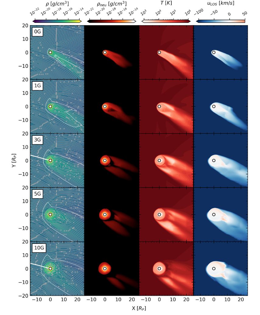
Figure 11: Behaviour of the planetary atmosphere during the interaction with magnetized stellar wind. The star is kept outside of the simulation grid and located at negative x. The stellar wind is entering from the left side into the simulation grid. The planet is kept at the center of the grid and marked by a circle. Each row shows different planetary magnetic dipole field strengths. The first column shows the total density profile. The grey contours show the velocity streamlines and the magnetosonic surface is shown in the white contour. The second, third, and fourth columns show neutral hydrogen density, temperature, and line-of-sight velocity of the planetary atmosphere. The figure is taken from Carolan et al (2021a)

The Ly-$\alpha$ transit calculation in their model shows an enhancement in line-center absorption with increasing planetary magnetic field strength, as more planetary materials are trapped in the increasing equatorial dead zone. The absorption in the blue wing due to high-velocity neutral was also found to be increasing with planetary field strength.

Some studies (e.g., Cohen et al, 2015; Dong et al, 2017) on the effect of magnetic field on the terrestrial exoplanets are also performed. Cohen et al (2015) performed a simulation of the interaction of magnetized stellar wind on the unmagnetized Venus-like planets and concluded that the stellar wind can penetrate very deep into the atmosphere and enhance the mass-loss rate. For proxima-centauri b, Dong et al (2017) reported that the mass-loss rates are lowered if the planet has an intrinsic dipole magnetic field. A detailed study of terrestrial exoplanets for the magnetic interaction of stellar wind with the planetary magnetosphere is needed. Also, special care is needed to interpret those results from transit observations which is missing from the present studies.

4.3 Impact of flares and Coronal Mass Ejections(CMEs) of host star on exoplanetary atmospheric escape

The flares and CMEs when occurring on the host star change the radiation, and plasma density of the outflowing wind from the host star. The modified radiation during flares from the host star changes the photochemistry and ionization level of the upper atmosphere of the planet. On the other hand, the CME enhances the dynamic pressure, charge exchanges, and collisional ionization on the planetary upper atmosphere. As a result, both of the events increase the planetary mass-loss rates. Hence the study of the effect of flares and CMEs on the planetary mass loss is very important and has been carried out by several groups (Segura et al, 2010; Venot et al, 2016; Kay et al, 2016; Chadney et al, 2017; Cherenkov et al, 2017; Bisikalo et al, 2018; Hazra et al, 2020; Louca et al, 2022; Hazra et al, 2022). The changes in the planetary mass-loss rate during the flares and CME would also change the observational signature temporarily. The Ly-$\alpha$ transit observations of HD189733b by Lecavelier des Etangs et al (2012) using STIS, HST in two epochs show an enhancement of transit depths in the second epoch compared to the first epoch. The first transit observation that was made in April 2010 showed a negligible transit depth. The second transit event in September 2011 showed an enhanced transit absorption depth of $14.4\pm 3.6\%$ between velocities of -230 to -140 km s^-1. At the second epoch, 8 hours before the transit observation, an X-ray flare from the star was also observed with Swift/XRT. These combined observations support the idea that the individual flare or flare-associated CME must have caused an enhanced mass loss from the upper atmosphere of the planet HD189733b (Guo and Ben-Jaffel, 2016; Chadney et al, 2017; Hazra et al, 2020, 2022).

For gaseous giant planets, Hazra et al (2020) analyzed the effect of flares on the upper atmosphere using a 1D escape model and found an enhancement of mass loss due to flaring events. The transit signatures in both Ly-$\alpha$ and H-$\alpha$ have been enhanced due to the flare on the host star. As the 1D model can not take into the interaction of stellar wind, the asymmetric high-velocity blue and red wings could not be modeled.

A more rigorous calculation of the effect of flare and CME on the planetary atmosphere of a hot Jupiter has been performed by Hazra et al (2022) using a 3D radiation-hydrodynamics model. They investigated four cases: first - stellar wind in the quiescent phase of the star, second - a flare, third - a CME, and fourth - a flare that is followed by a CME. The dynamics of the planetary atmosphere for these four cases are shown in figure 12. Each row shows different planetary properties. The total density, neutral density, temperature, and total velocity are shown from the first to the fourth row, respectively. Each column shows each of the considered four cases. The behavior of planetary materials is different for the four cases. The distinct difference arises when we consider the CME case. Comparison of the behavior of different atmosphere properties for case-1 and case-III clearly shows the difference in the cometary tail where materials are swept out by stellar wind and CME plasma respectively. For the flare case (case-II), the day-side sonic surface resides a bit higher than the quiescent stellar wind case (case-III) because of the higher rate of planetary outflow. The mass-loss rates for the four cases differ quite significantly. The flare case alone increases the mass-loss rate by 25% compared to the quiescent phase, while the CME leads to an increment by a factor of 4.

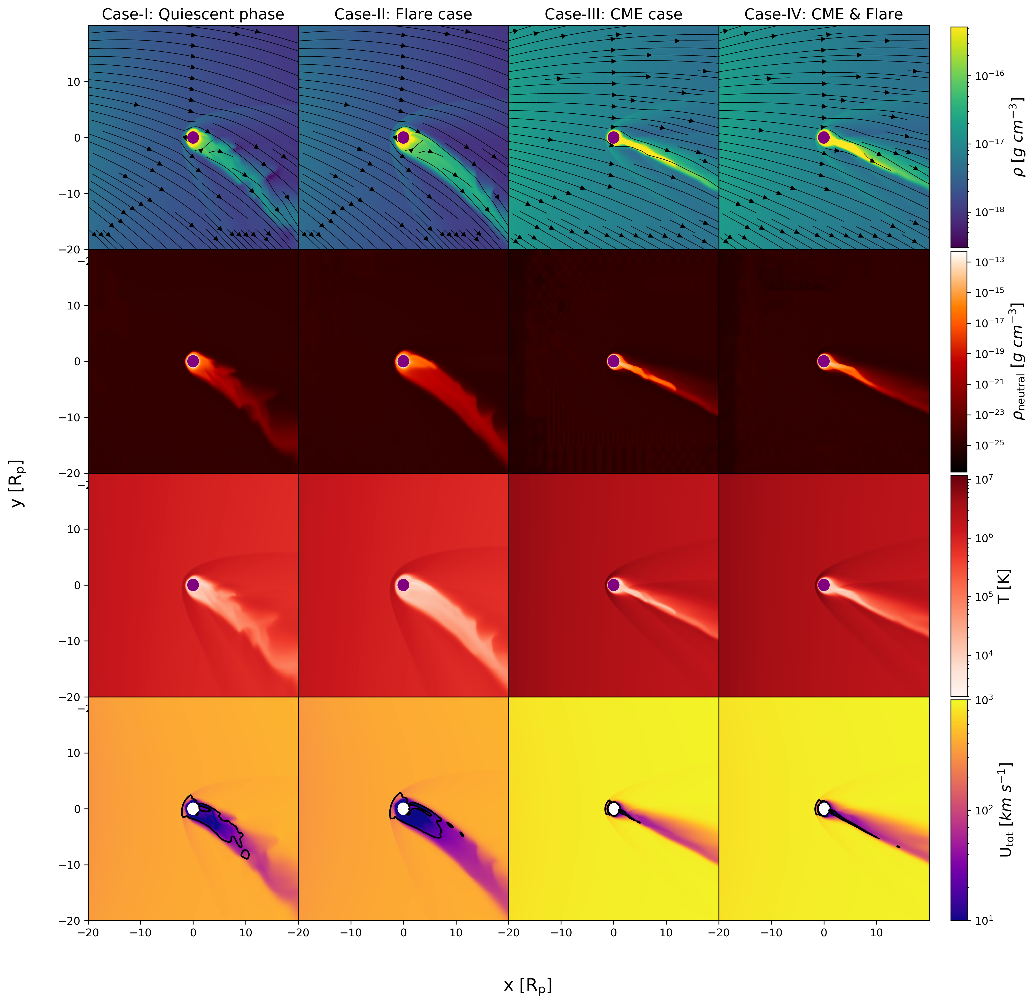
Figure 12: The behavior of the planetary atmosphere for the four cases is shown here. The first column shows the total density (first row), neutral density (second row), temperature (third row), and total velocity (fourth row) for the quiescent stellar wind case. The second column, third column, and fourth column show the same quantity in each row for case-II, case-III, and case-IV respectively. All the plots are shown in the orbital planes (z = 0).

The synthetic Ly-$\alpha$ simulated for the four cases mentioned above also show different transit absorption depths, which is shown in figure 13. The flare case, CME case, and CME + flare case are shown using green, magenta, and yellow lines respectively. The flare case increases the transit depth in the line center but the CME case increases the transit depth in the blue-wing (-230 to -140 km s^-1). Hence Hazra et al (2022) concluded that the observed enhanced transit depth in the second epoch of the transit measurement (Lecavelier des Etangs et al, 2012) is more likely due to a CME affecting the planetary atmosphere not due to the flare alone as argued before.

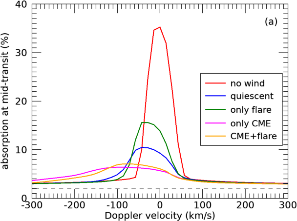
Figure 13: Synthetic Ly-$\alpha$ spectra calculated from planetary transit for four cases mentioned above. The blue, green, magenta, and yellow lines show the transit spectra for the quiescent case, flare case, CME case, and CME+flare case. The red line shows the transit spectra due to radiation-driven planetary outflow alone without any interaction with stellar wind

Louca et al (2022) has recently studied the effect of stellar flares on the chemistry of gas giants to terrestrial exoplanets. Significant changes are reported in the abundance of some relevant species such as H, OH, and CH₄. They reported the abundance changes up to three orders of magnitude in comparison to pre-flare abundances. Konings et al (2022) showed that the flares can affect the atmosphere of gas giants up to several days after the flare event during which the transmission spectra are altered by several hundred ppm. However, recently Gillet et al (2025) studied the effect of flares on gas giants considering a realistic temporal evolution of the XUV flux of a flare and found no effect of flares on mass-loss rate and Ly-$\alpha$ signature. Hence, to understand effect of flares on exoplanet atmospheres, more thorough studies are needed.

Most of the previous efforts to study the impact of CMEs on atmospheric escape were done using hydrodynamical models (e.g., Kay et al, 2016; Cherenkov et al, 2017; Hazra et al, 2022). Recently Hazra et al (2025) studied the magnetic interaction of CME plasma with the atmosphere of a hot Jupiter with dipolar magnetosphere using time-dependent radiative MHD simulations. They have considered three configurations of embedded CME magnetic field - (a) northward $B_{z}$ component, (b) southward $B_{z}$ component, and (c)radial component. They found that CMEs with both northward and southward $B_{z}$ are most effective in removing planetary material and hence escape rate. The planetary magnetosphere goes through three distinct changes while interacting with the CME. Interestingly, the maximum Ly-$\alpha$ transit absorption depth is found when the CME has a radial embedded field and less planetary escape rate.

4.4 A note on computing synthetic transit spectra from atmospheric escape models

To probe atmospheric escape from exoplanet observationally and constrain theoretical models, transit spectroscopy is the only reliable methodology available to us. As I explain in section  4, most of the numerical models (both 1D and multidimensional) compare their result every time with the transit spectra of Ly-$\alpha$, as atmospheric escape have been studied most in the hydrogen Ly-$\alpha$ line. There are also some theoretical models (e.g., Hazra et al, 2020; Mitani et al, 2022; Yan et al, 2022, 2024) that compare their simulated results with H-$\alpha$ transit observations. Hazra et al (2020) synthetically calculated H-$\alpha$ line for different XUV radiation during a magnetic cycle of host star and estimated a variation of 1.9 mÅ in equivalent width over the cycle. They also found that H-$\alpha$ increases during a flare case.Yan et al (2022) and Yan et al (2024) modelled WASP-52b and HAT-P-32b using 1D hydrodynamic model to compute the H-$\alpha$ transmission spectra combined with non local thermodynamic and Monte Carlo simulation. By comparing H-$\alpha$ observation with simulated H-$\alpha$ spectra, they show that it is possible to constrain the XUV radiation and metallicity of the atmosphere. Using 3D model Mitani et al (2022) computed H-$\alpha$ line due to the stellar wind interaction with the upper atmosphere of exoplanet and found a weak effect of stellar wind on H-$\alpha$ line. After the first detection of helium escaping a planet (Spake et al, 2018), constraining theoretical models using helium lines becomes relevant as the helium lines would help us to constrain the launching region of the planetary outflow. There are many 1D hydrodynamic escape models (e.g., Dos Santos et al, 2022; Lampón et al, 2020; Zhang et al, 2023; Lampón et al, 2023; Rosener et al, 2025) have been developed in the last few years which compute helium signals. However, 3D numerical models of helium escape modeling have been limited to date and we need more self-consistent 3D models. Another interesting constraint on the theoretical model might come from the modeling of transit spectra using metal lines, which also has not been done extensively. Although in the last few years, Ly-$\alpha$ transit observations gave us a lot of constraint on the mass-loss rate from exoplanets, with the discovery of helium and the possibility of detecting it from the ground based telescopes, helium triplet line could be used to probe the atmospheric escape widely. Actually, the most suitable things would be simultaneous modeling of hydrogen and helium lines and compare them with observations. Because of the contamination of Ly-$\alpha$ by interstellar medium and geo-emission, observing H-$\alpha$ and helium triplet line should be used as a complementary method for understanding evaporation from exoplanets (Czesla et al, 2022; Yan et al, 2022, 2024).

An important point to note while interpreting observed Ly-$\alpha$ absorption as the actual mass-loss rate is that Ly-$\alpha$ transit occurs due to the absorption of stellar Ly-$\alpha$ line by neutral hydrogen only. Hence Ly-$\alpha$ should give the mass-loss rate of neutral hydrogen. It does not give any information about the ionized hydrogen (proton) loss. Recent non-detection of Ly-$\alpha$ in many highly irradiated close-in exoplanets (HD97658b (Bourrier et al, 2017), $\pi$ Men C (García Muñoz et al, 2020), young planet K2-25b (Rockcliffe et al, 2021), HD63433b (Zhang et al, 2022b, the third planet HD63433c further away than the second planet HD63433b shows significant Ly-$\alpha$ absorption)) needs further attention and investigation as to why Ly-$\alpha$ will not always be an indicator for mass loss. Owen et al (2023) analysed the fundamentals of Ly-$\alpha$ transit to interpret the observation. They found that for Ly-$\alpha$ to be detected, the planetary material must be sufficiently radially accelerated before it gets too ionized. The too much ionization of the cometary tail might be the reason for several non-detections of Ly-$\alpha$ in the close-in planets. Along with the transit depth, the transit duration is very important as it encodes information about the progressive ionization of the cometary tail. Another alternative explanation of the non-detection of Ly-$\alpha$ is stellar wind confinement (Vidotto and Cleary, 2020; Carolan et al, 2021b). The stellar wind of the host star is so strong that it confines the planetary outflow to an undetected limit. These studies (Owen et al, 2023; Carolan et al, 2021b) make it clear that the non-detection of Ly-$\alpha$ does not mean that the planet is not going through atmospheric escape, nor is the planet hydrogen-dominated, rather it needs careful interpretation. Much more constraints could be imposed on the evaporating atmosphere if we observe the hydrogen and helium line simultaneously (Czesla et al, 2022; Bello-Arufe et al, 2023). Not only simultaneous observation will give us confirmation that the atmosphere is indeed evaporating but also it will help us constraining the H/He ratio in the atmosphere and the XUV radiation from the host star. Yan et al (2022) and Yan et al (2024) studied atmosphere of WASP-52b and HAT-P-32b in both H-$\alpha$ and helium triplet simultaneously. For WASP-52b, to match with the observation of both H-$\alpha$ and helium triplet, a high XUV radiation is needed with a low X-ray fraction in XUV radiation or less XUV radiation with high X-ray fraction with H/He ratio = 98/2 (Yan et al, 2022). For HAT-P-32b, they found a solar-like metallicity in the upper atmosphere (see Yan et al, 2024, for details). Nevertheless, in the near future, simultaneous modeling of hydrogen and helium lines will pave the way for understanding the evaporating atmosphere and its compositions.

5 Importance of atmospheric escape in the evolution of exoplanets

The atmospheric escape plays the most important role in atmospheric erosion which sometimes leads to the complete loss of the planetary atmosphere. Hence, to understand planetary atmospheric evolution, it is very important to understand the atmospheric escape mechanism properly. Some earlier studies (Khodachenko et al, 2007; Lammer et al, 2007) showed that the CME-driven atmospheric escape can strip off the whole atmosphere of unmagnetized exoplanets during a 1-Gyr period. With the recent discovery of radius gap (Fulton et al, 2017) and Neptunian desert (Mazeh et al, 2016) in the observed exoplanet demographics, studies of atmospheric evolution become very relevant, where evolution is invoked as one of the major reasons for these observed gaps in exoplanet demographics.

Recent studies have shown that the observed radius valley can be reproduced by incorporating atmospheric mass loss in the evolution by either photoevaporation or core-powered mass loss (Rogers et al, 2021). Hence direct evidence of atmospheric evolution is verified by reproducing the radius valley as observed. Similarly, for the Neptune-sized planet, atmospheric mass loss over time completely removed the atmosphere of the Neptune-sized planet and gave rise to the observed Neptunian desert (Ionov et al, 2018; Vissapragada et al, 2022). However, this atmospheric evolution estimation due to mass-loss by photoevaporation or core-powered has assumed a parametric mass-loss formula, which may not be accurate as it is not easy to discern which types (e.g., photon-limited, energy-limited, or radiation/recombination-limited) of atmospheric escape is going on in the planet. Also, as we describe in section 4.2, the stellar wind, stellar magnetic field, stellar flares, and CMEs play a very important role in mediating atmospheric mass-loss rate. To properly calculate atmospheric mass loss and its effect on overall planetary atmosphere evolution, we need to incorporate the full stellar environment and its interaction with the planetary atmosphere.

6 Future perspective and outlook

In this review, I summarise the atmospheric escape processes from exoplanets including the methodology of their observation and theoretical modeling to date. The atmospheric escape from exoplanets has been driven largely by stellar environments - such as stellar radiation, stellar wind, CMEs, and flares (Murray-Clay et al, 2009; Carroll-Nellenback et al, 2017; Hazra et al, 2022). Sometimes Core-powered energy that the planet acquires during the accretion phase of planet formation can also lead the atmospheric escape (Gupta and Schlichting, 2020), but direct observational evidence is far from constraining this mechanism.

One of the major driving forces of atmospheric escape from planets is stellar radiation (XUV radiation, infrared). The observational measurements of this important quantity are still in the very preliminary stage. We have measurements of the X-ray part but the extreme ultraviolet part of the stellar spectra is still observationally ill-constrained. The earlier efforts were to reconstruct the EUV part of the stellar spectra using empirical relations from X-ray (Chadney et al, 2015) and stellar Ly$\alpha$ (Sanz-Forcada et al, 2011). Recently there have been some efforts- MUSCLES Treasury Survey (France et al, 2016; Youngblood et al, 2016) and MEGA MUSCLES survey (Froning et al, 2019; France et al, 2020) to make a spectral database of many planet-hosting stars. In the MUSCLE survey, SEDs with a spectral range of 5 Å to 5.5 $\mu$m of 11 nearby planet-hosting stars (M-dwarfs and K-dwarfs) in the solar neighborhood (d $\leq$ 20 pc) have been carried out. The MUSCLE survey includes observations in visible wavelength from Hubble and ground-based observatory, X-rays from Chandra/XMM-Newton/Swift. Other wavelengths in infrared and astrophysically inaccessible wavelengths, EUV and Ly-$\alpha$ are reconstructed using empirical relations and stellar model spectra. Recently Mega-MUSCLE survey (France et al, 2020) added another 13 stars in the MUSCLE database. Behr et al (2023) extended the database by adding SEDs of 11 JWST targets. Although MUSCLE database provides SEDs of some important planet-hosting stars, we need more observations of SEDs from parent stars in the near future. Also, the reconstruction of the observationally inaccessible part of the spectra needs a better physics-constrained model instead of mere empirical scaling relations (e.g., Sanz-Forcada et al, 2011; Linsky et al, 2014).

Immediately after the stellar radiation, the most important quantity that affects the atmospheric escape (non-thermal loss) is the stellar wind. Depending upon the stellar wind strength, the mass-loss rate of the escaping atmosphere is decided (see section 4.2.1 for details). The strength of the stellar wind is approximated by the mass-loss rate from stars and observational quantification of this quantity would be very important for atmospheric escape calculation from exoplanets. By measuring astrospheric absorption signature produced by the interaction between the stellar winds and the interstellar medium, Wood et al (2021) estimated the mass-loss rate of M-dwarf stellar winds. The soft X-ray emission (produced by charge exchange between heavy ions of the stellar wind and cold neutrals of interstellar medium) from the stellar astrosphere is also another good detector of stellar wind mass-loss rate (Kislyakova et al, 2024). A detailed study of observational stellar wind with theoretical modeling is needed to constrain stellar wind strength, which will help to probe atmospheric escape from the planets appropriately.

Many numerical simulations (Lammer et al, 2007; Khodachenko et al, 2007; Kay et al, 2016; Bisikalo et al, 2018; Hazra et al, 2022; Odert et al, 2020; Hazra et al, 2025) showed that coronal mass ejections and flares can significantly alter (sometimes one order of magnitude) the escape rate from the planetary atmosphere. Observations of the physical properties of CMEs and their occurrence rate in planet-hosting stars would be the next important steps in understanding their effect on atmospheric escape. Recently Veronig et al (2021) detected coronal dimming associated with flares on cool stars, which paves the way for comprehensive characterizations and detection of stellar CMEs. As flares and CMEs are directly affecting the atmospheric escape, their higher occurrence rates would lead to higher atmospheric mass loss from the exoplanets, which is crucial for atmospheric evolution. For the young host stars, flares occur more frequently than the stars which are of solar ages (Audard et al, 2000; Maehara et al, 2015). However, for the stellar CME, we have no observational information on the occurrence rate. For the Sun, the CME occurrence rate varies from 0.5 per day near solar minima to $\sim$ 6 near solar maxima (Gopalswamy et al, 2003; Yashiro et al, 2004). Some of the studies (Drake et al, 2013; Odert et al, 2017) have shown that young and more active stars could have a higher rate of CME occurrence than the Sun but this needs further careful study.

Along with constraining stellar environments from observations, we need detailed observations to understand atmospheric escape processes on the planetary side too. As we explained details in section 3, the transit observations have given us atmospheric escape rates (eg., Vidal-Madjar et al, 2003, 2004; Fossati et al, 2010; Lecavelier des Etangs et al, 2012; Bourrier et al, 2016) from many exoplanets. However, the detailed atmospheric structure is yet to be probed from observations including the exobase location. Most of the observations were carried out using hydrogen Ly-$\alpha$ lines, which can not probe low-velocity escaping planetary materials. On the other hand, helium triplet and H-$\alpha$ lines can probe the low-velocity launching area of escaping materials and have advantage of being observed from the ground based telescopes. Hence we need a simultaneous measurement of the escaping atmosphere by both helium and H-$\alpha$ transit lines in the near future for details understanding of the atmospheric escape. A combined Ly-$\alpha$ measurement along with H-$\alpha$ and helium line would be appropriate to constrain the H/He ratio in the atmosphere and the stellar XUV radiation.

Theoretical models for atmospheric escape are becoming mature with time. Atmospheric escape is an inherently 3D phenomenon and modeling them using 1D models would simplify many features, however, for the long-term planetary evolution studies, 1D models have been very helpful (Kubyshkina et al, 2018a; Johnstone et al, 2018; Allan and Vidotto, 2019). In the 3D modeling, the inclusion of multispecies (e.g., Hydrogen, Helium, Oxygen, Carbon, etc) definitely would help for the interpretation of the observed transit spectra and underlying physics, which is an ongoing effort (Dong et al, 2018; Hazra et al, 2022, 2025). However, in the presence of a magnetic field on the planet, different ionized species would behave differently with different velocities, and developing multi-fluid models would be the ultimate goal for a sophisticated atmospheric escape model. There are some efforts in this direction using 1D multifluid models (e.g., Guo, 2019; Xing et al, 2023). While studying water escape from terrestrial exoplanet using a 1D multifluid model, Guo (2019) found that the critical XUV value might be increased to a factor of 2 in case we neglect the ion momentum transfer, as ions effectively transfer momentum between interacting species. This multifluid model also helps us explain the mass fractionalization of helium in the escaping atmosphere of hot Jupiter HD209458b (Xing et al, 2023). Multidimensional multifluid models will help to understand charge exchanges (Esquivel et al, 2019) by stellar wind/CME plasma with the planetary materials and pick up ions by stellar wind. For the modeling of atmospheric escape from rocky exoplanets, we may sometimes need to go beyond fluid codes and use fully kinetic or hybrid codes to model atmospheric escape and its interaction with stellar wind (e.g., Jarvinen et al, 2018).

With the improved observations and modeling, we are progressing towards an understanding of atmospheric escape, but many questions remain due to the severe complexity involved in the atmospheric escape process. One of the main questions is related to radiative transfer modeling of incident stellar radiation. For the tidally locked exoplanets, the plane parallel approximation of radiation might not be a bad approximation but in the case of non-tidally locked planets, a better treatment of incident radiation is necessary. Yan et al (2022) for the first time performed transmission spectroscopy using a spherical stellar Ly-$\alpha$ radiation source. They found that plane-parallel illumination models overestimate the Ly-$\alpha$ strength for the plane planetary atmosphere and underestimate for spherical planetary atmosphere in comparison to those for the spherically illuminated models.

The coupling between the lower atmosphere and upper atmosphere should also be carefully considered as the abundance of various species in the upper atmosphere also depends on their values in the lower atmosphere. The role of the planetary magnetic field in atmospheric escape is very important and needs further study in the near future. Whether a planet with a magnetic field can protect an atmosphere from escaping or help the atmosphere in escaping - this conundrum needs to be tackled with details numerical modeling, which will include different values of planetary magnetic field and their different orientation of magnetosphere. is the role of the planetary magnetic field different for gaseous exoplanets to rocky exoplanets? In hindsight, a combination of observational studies along with self-consistent 3D radiative MHD or kinetic modeling of atmospheric escape is the key to solving many unresolved mysteries of atmospheric escape from exoplanets.

Acknowledgements The author thanks two anonymous referees for their constructive comments that helped a lot to improve the manuscript. The author would also like to thank Prof. Mitsuru Kikuchi for his kind invitation to write this review. The author also acknowledges the IIT Kanpur initiation grant (IITK/PHY/2022386) for financial support.

Declarations

Conflict of interest The author declares no conflict of interest

References

- \bibcommenthead
- Allan and Vidotto (2019) Allan A, Vidotto AA (2019) Evolution of atmospheric escape in close-in giant planets and their associated Ly and H transit predictions. Mon. Not. R. Astron. Soc.490(3):3760–3771. 10.1093/mnras/stz2842, https://arxiv.org/abs/arXiv:1908.03510 [astro-ph.EP]
- Allart et al (2018) Allart R, Bourrier V, Lovis C, et al (2018) Spectrally resolved helium absorption from the extended atmosphere of a warm Neptune-mass exoplanet. Science 362(6421):1384–1387. 10.1126/science.aat5879, https://arxiv.org/abs/arXiv:1812.02189 [astro-ph.EP]
- Allart et al (2023) Allart R, Lemée-Joliecoeur PB, Jaziri AY, et al (2023) Homogeneous search for helium in the atmosphere of 11 gas giant exoplanets with SPIRou. Astron. Astrophys.677:A164. 10.1051/0004-6361/202245832, https://arxiv.org/abs/arXiv:2307.05580 [astro-ph.EP]
- Alonso-Floriano et al (2019) Alonso-Floriano FJ, Snellen IAG, Czesla S, et al (2019) He I 10 830 Å in the transmission spectrum of HD209458 b. Astron. Astrophys.629:A110. 10.1051/0004-6361/201935979, https://arxiv.org/abs/arXiv:1907.13425 [astro-ph.EP]
- Audard et al (2000) Audard M, Güdel M, Drake JJ, et al (2000) Extreme-Ultraviolet Flare Activity in Late-Type Stars. Astrophys. J.541(1):396–409. 10.1086/309426, https://arxiv.org/abs/arXiv:astro-ph/0005062 [astro-ph]
- Barnes et al (2016) Barnes JR, Haswell CA, Staab D, et al (2016) The origin of the excess transit absorption in the HD 189733 system: planet or star? Mon. Not. R. Astron. Soc.462(1):1012–1028. 10.1093/mnras/stw1713, https://arxiv.org/abs/arXiv:1607.03684 [astro-ph.EP]
- Bear and Soker (2011) Bear E, Soker N (2011) Evaporation of Jupiter-like planets orbiting extreme horizontal branch stars. Mon. Not. R. Astron. Soc.414(2):1788–1792. 10.1111/j.1365-2966.2011.18527.x, https://arxiv.org/abs/arXiv:1102.5487 [astro-ph.SR]
- Behr et al (2023) Behr PR, France K, Brown A, et al (2023) The MUSCLES Extension for Atmospheric Transmission Spectroscopy: UV and X-Ray Host-star Observations for JWST ERS & GTO Targets. Astronimcal. J166(1):35. 10.3847/1538-3881/acdb70, https://arxiv.org/abs/arXiv:2306.05322 [astro-ph.SR]
- Bello-Arufe et al (2023) Bello-Arufe A, Knutson HA, Mendonça JM, et al (2023) Transmission Spectroscopy of the Lowest-density Gas Giant: Metals and a Potential Extended Outflow in HAT-P-67b. Astronimcal. J166(2):69. 10.3847/1538-3881/acd935, https://arxiv.org/abs/arXiv:2307.06356 [astro-ph.EP]
- Ben-Jaffel et al (2022) Ben-Jaffel L, Ballester GE, García Muñoz A, et al (2022) Signatures of strong magnetization and a metal-poor atmosphere for a Neptune-sized exoplanet. Nature Astronomy 6:141–153. 10.1038/s41550-021-01505-x, https://arxiv.org/abs/arXiv:2211.05155 [astro-ph.EP]
- Biassoni et al (2024) Biassoni F, Caldiroli A, Gallo E, et al (2024) Self-consistent modeling of metastable helium exoplanet transits. Astron. Astrophys.682:A115. 10.1051/0004-6361/202347517, https://arxiv.org/abs/arXiv:2310.13052 [astro-ph.EP]
- Bisikalo et al (2018) Bisikalo DV, Shematovich VI, Cherenkov AA, et al (2018) Atmospheric Mass Loss from Hot Jupiters Irradiated by Stellar Superflares. Astrophys. J.869(2):108. 10.3847/1538-4357/aaed21, https://arxiv.org/abs/arXiv:1811.02303 [astro-ph.EP]
- Bouhram et al (2004) Bouhram M, Klecker B, Paschmann G, et al (2004) Multipoint analysis of the spatio-temporal coherence of dayside O+ outflows with Cluster. Annales Geophysicae 22(7):2507–2514. 10.5194/angeo-22-2507-2004
- Bourrier et al (2016) Bourrier V, Lecavelier des Etangs A, Ehrenreich D, et al (2016) An evaporating planet in the wind: stellar wind interactions with the radiatively braked exosphere of GJ 436 b. Astron. Astrophys.591:A121. 10.1051/0004-6361/201628362, https://arxiv.org/abs/arXiv:1605.07973 [astro-ph.EP]
- Bourrier et al (2017) Bourrier V, Ehrenreich D, King G, et al (2017) No hydrogen exosphere detected around the super-Earth HD 97658 b. Astron. Astrophys.597:A26. 10.1051/0004-6361/201629253, https://arxiv.org/abs/arXiv:1609.04416 [astro-ph.EP]
- Bourrier et al (2018) Bourrier V, Lecavelier des Etangs A, Ehrenreich D, et al (2018) Hubble PanCET: an extended upper atmosphere of neutral hydrogen around the warm Neptune GJ 3470b. Astron. Astrophys.620:A147. 10.1051/0004-6361/201833675, https://arxiv.org/abs/arXiv:1812.05119 [astro-ph.EP]
- Brain et al (2016) Brain DA, Bagenal F, Ma YJ, et al (2016) Atmospheric escape from unmagnetized bodies. Journal of Geophysical Research (Planets) 121(12):2364–2385. 10.1002/2016JE005162
- Carolan et al (2020) Carolan S, Vidotto AA, Plavchan P, et al (2020) The dichotomy of atmospheric escape in AU Mic b. Mon. Not. R. Astron. Soc.498(1):L53–L57. 10.1093/mnrasl/slaa127, https://arxiv.org/abs/arXiv:2006.13606 [astro-ph.EP]
- Carolan et al (2021a) Carolan S, Vidotto AA, Hazra G, et al (2021a) The effects of magnetic fields on observational signatures of atmospheric escape in exoplanets: Double tail structures. Mon. Not. R. Astron. Soc.508(4):6001–6012. 10.1093/mnras/stab2947, https://arxiv.org/abs/arXiv:2110.05200 [astro-ph.EP]
- Carolan et al (2021b) Carolan S, Vidotto AA, Villarreal D’Angelo C, et al (2021b) Effects of the stellar wind on the Ly transit of close-in planets. Mon. Not. R. Astron. Soc.500(3):3382–3393. 10.1093/mnras/staa3431, https://arxiv.org/abs/arXiv:2010.15094 [astro-ph.EP]
- Carroll-Nellenback et al (2017) Carroll-Nellenback J, Frank A, Liu B, et al (2017) Hot planetary winds near a star: dynamics, wind-wind interactions, and observational signatures. Mon. Not. R. Astron. Soc.466(2):2458–2473. 10.1093/mnras/stw3307, https://arxiv.org/abs/arXiv:1604.08532 [astro-ph.EP]
- Cauley et al (2017) Cauley PW, Redfield S, Jensen AG (2017) A Decade of H Transits for HD 189733 b: Stellar Activity versus Absorption in the Extended Atmosphere. Astronimcal. J153(5):217. 10.3847/1538-3881/aa6a15, https://arxiv.org/abs/arXiv:1703.09543 [astro-ph.EP]
- Chadney et al (2015) Chadney JM, Galand M, Unruh YC, et al (2015) XUV-driven mass loss from extrasolar giant planets orbiting active stars. ICARUS250:357–367. 10.1016/j.icarus.2014.12.012, https://arxiv.org/abs/arXiv:1412.3380 [astro-ph.SR]
- Chadney et al (2017) Chadney JM, Koskinen TT, Galand M, et al (2017) Effect of stellar flares on the upper atmospheres of HD 189733b and HD 209458b. Astron. Astrophys.608:A75. 10.1051/0004-6361/201731129, https://arxiv.org/abs/arXiv:1710.08365 [astro-ph.EP]
- Chaffin et al (2014) Chaffin MS, Chaufray JY, Stewart I, et al (2014) Unexpected variability of Martian hydrogen escape. Geophys. Res. Lett.41(2):314–320. 10.1002/2013GL058578
- Chamberlain (1963) Chamberlain JW (1963) Planetary coronae and atmospheric evaporation. Planetary and Space Science11(8):901–960. 10.1016/0032-0633(63)90122-3
- Chamberlain and Smith (1971) Chamberlain JW, Smith GR (1971) Comments on the rate of evaporation of a non-Maxwellian atmosphere. Planetary and Space Science19(7):675–684. 10.1016/0032-0633(71)90025-0
- Cherenkov et al (2017) Cherenkov A, Bisikalo D, Fossati L, et al (2017) The Influence of Coronal Mass Ejections on the Mass-loss Rates of Hot-Jupiters. Astrophys. J.846(1):31. 10.3847/1538-4357/aa82b2, https://arxiv.org/abs/arXiv:1709.01027 [astro-ph.EP]
- Christie et al (2016) Christie D, Arras P, Li ZY (2016) Axisymmetric Simulations of Hot Jupiter-Stellar Wind Hydrodynamic Interaction. Astrophys. J.820(1):3. 10.3847/0004-637X/820/1/3, https://arxiv.org/abs/arXiv:1601.05302 [astro-ph.EP]
- Cloutier (2024) Cloutier R (2024) Exoplanet Demographics: Physical and Orbital Properties. arXiv e-prints arXiv:2409.13062. 10.48550/arXiv.2409.13062, https://arxiv.org/abs/arXiv:2409.13062 [astro-ph.EP]
- Cohen et al (2011) Cohen O, Kashyap VL, Drake JJ, et al (2011) The Dynamics of Stellar Coronae Harboring Hot Jupiters. I. A Time-dependent Magnetohydrodynamic Simulation of the Interplanetary Environment in the HD 189733 Planetary System. Astrophys. J.733(1):67. 10.1088/0004-637X/733/1/67, https://arxiv.org/abs/arXiv:1101.4825 [astro-ph.SR]
- Cohen et al (2015) Cohen O, Ma Y, Drake JJ, et al (2015) The Interaction of Venus-like, M-dwarf Planets with the Stellar Wind of Their Host Star. Astrophys. J.806(1):41. 10.1088/0004-637X/806/1/41, https://arxiv.org/abs/arXiv:1504.06326 [astro-ph.EP]
- Cubillos et al (2020) Cubillos PE, Fossati L, Koskinen T, et al (2020) Near-ultraviolet Transmission Spectroscopy of HD 209458b: Evidence of Ionized Iron Beyond the Planetary Roche Lobe. Astronimcal. J159(3):111. 10.3847/1538-3881/ab6a0b, https://arxiv.org/abs/arXiv:2001.03126 [astro-ph.EP]
- Cui et al (2008) Cui J, Yelle RV, Volk K (2008) Distribution and escape of molecular hydrogen in Titan’s thermosphere and exosphere. Journal of Geophysical Research (Planets) 113(E10):E10004. 10.1029/2007JE003032
- Czesla et al (2022) Czesla S, Lampón M, Sanz-Forcada J, et al (2022) H and He I absorption in HAT-P-32 b observed with CARMENES. Detection of Roche lobe overflow and mass loss. Astron. Astrophys.657:A6. 10.1051/0004-6361/202039919, https://arxiv.org/abs/arXiv:2110.13582 [astro-ph.EP]
- Damon (1957) Damon PE (1957) Terrestrial helium. Geochimica et Cosmochimica Acta11(3):200–201. 10.1016/0016-7037(57)90084-4
- Debrecht et al (2020) Debrecht A, Carroll-Nellenback J, Frank A, et al (2020) Effects of radiation pressure on the evaporative wind of HD 209458b. Mon. Not. R. Astron. Soc.493(1):1292–1305. 10.1093/mnras/staa351, https://arxiv.org/abs/arXiv:1906.00075 [astro-ph.EP]
- Dong et al (2017) Dong C, Lingam M, Ma Y, et al (2017) Is Proxima Centauri b Habitable? A Study of Atmospheric Loss. Astrophys. J. Lett.837(2):L26. 10.3847/2041-8213/aa6438, https://arxiv.org/abs/arXiv:1702.04089 [astro-ph.EP]
- Dong et al (2018) Dong C, Jin M, Lingam M, et al (2018) Atmospheric escape from the TRAPPIST-1 planets and implications for habitability. Proceedings of the National Academy of Science 115(2):260–265. 10.1073/pnas.1708010115, https://arxiv.org/abs/arXiv:1705.05535 [astro-ph.EP]
- Dong et al (2019) Dong C, Huang Z, Lingam M (2019) Role of Planetary Obliquity in Regulating Atmospheric Escape: G-dwarf versus M-dwarf Earth-like Exoplanets. Astrophys. J. Lett.882(2):L16. 10.3847/2041-8213/ab372c, https://arxiv.org/abs/arXiv:1907.07459 [astro-ph.EP]
- dos Santos et al (2019) dos Santos LA, Bourrier V, Ehrenreich D, et al (2019) Observability of hydrogen-rich exospheres in Earth-like exoplanets. Astron. Astrophys.622:A46. 10.1051/0004-6361/201833392, https://arxiv.org/abs/arXiv:1812.02145 [astro-ph.EP]
- Dos Santos et al (2022) Dos Santos LA, Vidotto AA, Vissapragada S, et al (2022) p-winds: An open-source Python code to model planetary outflows and upper atmospheres. Astron. Astrophys.659:A62. 10.1051/0004-6361/202142038, https://arxiv.org/abs/arXiv:2111.11370 [astro-ph.EP]
- Drake et al (2013) Drake JJ, Cohen O, Yashiro S, et al (2013) Implications of Mass and Energy Loss due to Coronal Mass Ejections on Magnetically Active Stars. Astrophys. J.764(2):170. 10.1088/0004-637X/764/2/170, https://arxiv.org/abs/arXiv:1302.1136 [astro-ph.SR]
- Dubinin et al (2011) Dubinin E, Fraenz M, Fedorov A, et al (2011) Ion Energization and Escape on Mars and Venus. Space Science Rev.162(1-4):173–211. 10.1007/s11214-011-9831-7
- Ehrenreich and Désert (2011) Ehrenreich D, Désert JM (2011) Mass-loss rates for transiting exoplanets. Astron. Astrophys.529:A136. 10.1051/0004-6361/201016356, https://arxiv.org/abs/arXiv:1103.0011 [astro-ph.EP]
- Ehrenreich et al (2015) Ehrenreich D, Bourrier V, Wheatley PJ, et al (2015) A giant comet-like cloud of hydrogen escaping the warm Neptune-mass exoplanet GJ 436b. Nature522(7557):459–461. 10.1038/nature14501, https://arxiv.org/abs/arXiv:1506.07541 [astro-ph.EP]
- Erkaev et al (2015) Erkaev NV, Lammer H, Odert P, et al (2015) Extreme hydrodynamic atmospheric loss near the critical thermal escape regime. Mon. Not. R. Astron. Soc.448(2):1916–1921. 10.1093/mnras/stv130, https://arxiv.org/abs/arXiv:1506.06592 [astro-ph.EP]
- Esquivel et al (2009) Esquivel A, Raga AC, Cantó J, et al (2009) The interaction of an O star wind with a Herbig-Haro jet. A&A 507:855–860. 10.1051/0004-6361/200912825
- Esquivel et al (2019) Esquivel A, Schneiter M, Villarreal D’Angelo C, et al (2019) Hydrodynamical interaction of stellar and planetary winds: effects of charge exchange and radiation pressure on the observed Ly absorption. Mon. Not. R. Astron. Soc.487(4):5788–5798. 10.1093/mnras/stz1725, https://arxiv.org/abs/arXiv:1907.04933 [astro-ph.EP]
- Fossati et al (2010) Fossati L, Haswell CA, Froning CS, et al (2010) Metals in the Exosphere of the Highly Irradiated Planet WASP-12b. Astrophys. J. Lett.714(2):L222–L227. 10.1088/2041-8205/714/2/L222, https://arxiv.org/abs/arXiv:1005.3656 [astro-ph.SR]
- France et al (2016) France K, Loyd ROP, Youngblood A, et al (2016) The MUSCLES Treasury Survey. I. Motivation and Overview. Astrophys. J.820(2):89. 10.3847/0004-637X/820/2/89, https://arxiv.org/abs/arXiv:1602.09142 [astro-ph.SR]
- France et al (2017) France K, Fleming B, West G, et al (2017) The LUVOIR Ultraviolet Multi-Object Spectrograph (LUMOS): instrument definition and design. In: Siegmund OH (ed) Society of Photo-Optical Instrumentation Engineers (SPIE) Conference Series, p 1039713, 10.1117/12.2272025, 1709.06141
- France et al (2020) France K, Duvvuri G, Egan H, et al (2020) The High-energy Radiation Environment around a 10 Gyr M Dwarf: Habitable at Last? Astronimcal. J160(5):237. 10.3847/1538-3881/abb465, https://arxiv.org/abs/arXiv:2009.01259 [astro-ph.EP]
- Froning et al (2019) Froning CS, Kowalski A, France K, et al (2019) A Hot Ultraviolet Flare on the M Dwarf Star GJ 674. Astrophys. J. Lett.871(2):L26. 10.3847/2041-8213/aaffcd, https://arxiv.org/abs/arXiv:1901.08647 [astro-ph.SR]
- Fulton et al (2017) Fulton BJ, Petigura EA, Howard AW, et al (2017) The California-Kepler Survey. III. A Gap in the Radius Distribution of Small Planets. Astronimcal. J154(3):109. 10.3847/1538-3881/aa80eb, https://arxiv.org/abs/arXiv:1703.10375 [astro-ph.EP]
- García Muñoz (2007) García Muñoz A (2007) Physical and chemical aeronomy of HD 209458b. Planetary and Space Science55(10):1426–1455. 10.1016/j.pss.2007.03.007
- García Muñoz et al (2020) García Muñoz A, Youngblood A, Fossati L, et al (2020) Is Men c’s Atmosphere Hydrogen-dominated? Insights from a Non-detection of H I Ly Absorption. Astrophys. J. Lett.888(2):L21. 10.3847/2041-8213/ab61ff, https://arxiv.org/abs/arXiv:1912.06913 [astro-ph.EP]
- Garcia-Sage et al (2017) Garcia-Sage K, Glocer A, Drake JJ, et al (2017) On the Magnetic Protection of the Atmosphere of Proxima Centauri b. Astrophys. J. Lett.844(1):L13. 10.3847/2041-8213/aa7eca
- Gillet et al (2025) Gillet A, Strugarek A, García Muñoz A (2025) Secondary ionisation in hot atmospheres and interactions between planetary and stellar winds. arXiv e-prints arXiv:2502.08316. 10.48550/arXiv.2502.08316, https://arxiv.org/abs/arXiv:2502.08316 [astro-ph.EP]
- Ginzburg et al (2018) Ginzburg S, Schlichting HE, Sari R (2018) Core-powered mass-loss and the radius distribution of small exoplanets. Mon. Not. R. Astron. Soc.476(1):759–765. 10.1093/mnras/sty290, https://arxiv.org/abs/arXiv:1708.01621 [astro-ph.EP]
- Gopalswamy et al (2003) Gopalswamy N, Lara A, Yashiro S, et al (2003) Coronal mass ejection activity during solar cycle 23. In: Wilson A (ed) Solar Variability as an Input to the Earth’s Environment, pp 403–414
- Gronoff et al (2007) Gronoff G, Lilensten J, Simon C, et al (2007) Modelling dications in the diurnal ionosphere of Venus. Astron. Astrophys.465(2):641–645. 10.1051/0004-6361:20065991
- Gronoff et al (2008) Gronoff G, Lilensten J, Simon C, et al (2008) Modelling the Venusian airglow. Astron. Astrophys.482(3):1015–1029. 10.1051/0004-6361:20077503
- Gronoff et al (2020) Gronoff G, Arras P, Baraka S, et al (2020) Atmospheric Escape Processes and Planetary Atmospheric Evolution. Journal of Geophysical Research (Space Physics) 125(8):e27639. 10.1029/2019JA02763910.1002/essoar.10502458.1
- Gu et al (2023) Gu H, Wu X, Huang X, et al (2023) Nonthermal Atmospheric Escape on the Kepler-11 “Super-Earths” Driven by Stellar Wind Sputtering. Astrophys. J.959(2):80. 10.3847/1538-4357/ad0a84
- Guilluy et al (2023) Guilluy G, Bourrier V, Jaziri Y, et al (2023) DREAM: III. A helium survey in exoplanets on the edge of the hot Neptune desert with GIANO-B at TNG. Astron. Astrophys.676:A130. 10.1051/0004-6361/202346419, https://arxiv.org/abs/arXiv:2307.00967 [astro-ph.EP]
- Gunell et al (2018) Gunell H, Maggiolo R, Nilsson H, et al (2018) Why an intrinsic magnetic field does not protect a planet against atmospheric escape. Astron. Astrophys.614:L3. 10.1051/0004-6361/201832934
- Guo (2011) Guo JH (2011) Escaping Particle Fluxes in the Atmospheres of Close-in Exoplanets. I. Model of Hydrogen. Astrophys. J.733(2):98. 10.1088/0004-637X/733/2/98, https://arxiv.org/abs/arXiv:1103.2583 [astro-ph.EP]
- Guo (2019) Guo JH (2019) The Effect of Photoionization on the Loss of Water of the Planet. Astrophys. J.872(1):99. 10.3847/1538-4357/aaffd4
- Guo (2024) Guo JH (2024) Characterization of the regimes of hydrodynamic escape from low-mass exoplanets. Nature Astronomy 10.1038/s41550-024-02269-w, https://arxiv.org/abs/arXiv:2405.13283 [astro-ph.EP]
- Guo and Ben-Jaffel (2016) Guo JH, Ben-Jaffel L (2016) The Influence of the Extreme Ultraviolet Spectral Energy Distribution on the Structure and Composition of the Upper Atmosphere of Exoplanets. Astrophys. J.818(2):107. 10.3847/0004-637X/818/2/107, https://arxiv.org/abs/arXiv:1512.06470 [astro-ph.EP]
- Gupta and Schlichting (2020) Gupta A, Schlichting HE (2020) Signatures of the core-powered mass-loss mechanism in the exoplanet population: dependence on stellar properties and observational predictions. Mon. Not. R. Astron. Soc.493(1):792–806. 10.1093/mnras/staa315, https://arxiv.org/abs/arXiv:1907.03732 [astro-ph.EP]
- Hazra et al (2020) Hazra G, Vidotto AA, D’Angelo CV (2020) Influence of the Sun-like magnetic cycle on exoplanetary atmospheric escape. Mon. Not. R. Astron. Soc.496(3):4017–4031. 10.1093/mnras/staa1815, https://arxiv.org/abs/arXiv:2006.10634 [astro-ph.SR]
- Hazra et al (2022) Hazra G, Vidotto AA, Carolan S, et al (2022) The impact of coronal mass ejections and flares on the atmosphere of the hot Jupiter HD189733b. Mon. Not. R. Astron. Soc.509(4):5858–5871. 10.1093/mnras/stab3271, https://arxiv.org/abs/arXiv:2111.04531 [astro-ph.EP]
- Hazra et al (2025) Hazra G, Vidotto AA, Carolan S, et al (2025) Magnetic interaction of stellar coronal mass ejections with close-in exoplanets: implication on planetary mass-loss and Ly transits. Mon. Not. R. Astron. Soc.536(2):1089–1103. 10.1093/mnras/stae2559, https://arxiv.org/abs/arXiv:2411.06283 [astro-ph.SR]
- Huang et al (2023) Huang C, Koskinen T, Lavvas P, et al (2023) A hydrodynamic study of the escape of metal species and excited hydrogen from the atmosphere of the hot jupiter wasp-121b. The Astrophysical Journal 951(2):123. 10.3847/1538-4357/accd5e, URL https://dx.doi.org/10.3847/1538-4357/accd5e
- Ionov et al (2018) Ionov DE, Pavlyuchenkov YN, Shematovich VI (2018) Survival of a planet in short-period Neptunian desert under effect of photoevaporation. Mon. Not. R. Astron. Soc.476(4):5639–5644. 10.1093/mnras/sty626, https://arxiv.org/abs/arXiv:1803.04278 [astro-ph.EP]
- Jarvinen et al (2018) Jarvinen R, Brain DA, Modolo R, et al (2018) Oxygen Ion Energization at Mars: Comparison of MAVEN and Mars Express Observations to Global Hybrid Simulation. Journal of Geophysical Research (Space Physics) 123(2):1678–1689. 10.1002/2017JA024884
- Jensen et al (2012) Jensen AG, Redfield S, Endl M, et al (2012) A Detection of H in an Exoplanetary Exosphere. Astrophys. J.751(2):86. 10.1088/0004-637X/751/2/86, https://arxiv.org/abs/arXiv:1203.4484 [astro-ph.EP]
- Johnstone (2020) Johnstone CP (2020) Hydrodynamic Escape of Water Vapor Atmospheres near Very Active Stars. Astrophys. J.890(1):79. 10.3847/1538-4357/ab6224, https://arxiv.org/abs/arXiv:1912.07027 [astro-ph.EP]
- Johnstone et al (2015) Johnstone CP, Güdel M, Stökl A, et al (2015) The Evolution of Stellar Rotation and the Hydrogen Atmospheres of Habitable-zone Terrestrial Planets. Astrophys. J. Lett.815(1):L12. 10.1088/2041-8205/815/1/L12, https://arxiv.org/abs/arXiv:1511.03647 [astro-ph.EP]
- Johnstone et al (2018) Johnstone CP, Güdel M, Lammer H, et al (2018) Upper atmospheres of terrestrial planets: Carbon dioxide cooling and the Earth’s thermospheric evolution. Astron. Astrophys.617:A107. 10.1051/0004-6361/201832776, https://arxiv.org/abs/arXiv:1806.06897 [astro-ph.EP]
- Kay et al (2016) Kay C, Opher M, Kornbleuth M (2016) Probability of CME Impact on Exoplanets Orbiting M Dwarfs and Solar-like Stars. Astrophys. J.826(2):195. 10.3847/0004-637X/826/2/195, https://arxiv.org/abs/arXiv:1605.02683 [astro-ph.SR]
- Khodachenko et al (2007) Khodachenko ML, Ribas I, Lammer H, et al (2007) Coronal Mass Ejection (CME) Activity of Low Mass M Stars as An Important Factor for The Habitability of Terrestrial Exoplanets. I. CME Impact on Expected Magnetospheres of Earth-Like Exoplanets in Close-In Habitable Zones. Astrobiology 7(1):167–184. 10.1089/ast.2006.0127
- Khodachenko et al (2015) Khodachenko ML, Shaikhislamov IF, Lammer H, et al (2015) Atmosphere Expansion and Mass Loss of Close-orbit Giant Exoplanets Heated by Stellar XUV. II. Effects of Planetary Magnetic Field; Structuring of Inner Magnetosphere. Astrophys. J.813(1):50. 10.1088/0004-637X/813/1/50, https://arxiv.org/abs/arXiv:1711.04443 [astro-ph.EP]
- Khodachenko et al (2021) Khodachenko ML, Shaikhislamov IF, Fossati L, et al (2021) Simulation of 10 830 Å absorption with a 3D hydrodynamic model reveals the solar He abundance in upper atmosphere of WASP-107b. Mon. Not. R. Astron. Soc.503(1):L23–L27. 10.1093/mnrasl/slab015, https://arxiv.org/abs/arXiv:2101.12504 [astro-ph.EP]
- Kislyakova et al (2024) Kislyakova KG, Güdel M, Koutroumpa D, et al (2024) X-ray detection of astrospheres around three main-sequence stars and their mass-loss rates. Nature Astronomy 8:596–605. 10.1038/s41550-024-02222-x, https://arxiv.org/abs/arXiv:2404.14980 [astro-ph.SR]
- Konings et al (2022) Konings T, Baeyens R, Decin L (2022) Impact of stellar flares on the chemical composition and transmission spectra of gaseous exoplanets orbiting M dwarfs. Astron. Astrophys.667:A15. 10.1051/0004-6361/202243436, https://arxiv.org/abs/arXiv:2209.02483 [astro-ph.EP]
- Koskinen et al (2007) Koskinen TT, Aylward AD, Smith CGA, et al (2007) A Thermospheric Circulation Model for Extrasolar Giant Planets. Astrophys. J.661(1):515–526. 10.1086/513594
- Koskinen et al (2013) Koskinen TT, Harris MJ, Yelle RV, et al (2013) The escape of heavy atoms from the ionosphere of HD209458b. I. A photochemical-dynamical model of the thermosphere. ICARUS226(2):1678–1694. 10.1016/j.icarus.2012.09.027, https://arxiv.org/abs/arXiv:1210.1536 [astro-ph.EP]
- Krishnamurthy and Cowan (2024) Krishnamurthy V, Cowan NB (2024) Helium in Exoplanet Exospheres: Orbital and Stellar Influences. Astronimcal. J168(1):30. 10.3847/1538-3881/ad5441, https://arxiv.org/abs/arXiv:2403.15575 [astro-ph.EP]
- Kubyshkina et al (2018a) Kubyshkina D, Fossati L, Erkaev NV, et al (2018a) Overcoming the Limitations of the Energy-limited Approximation for Planet Atmospheric Escape. Astrophys. J. Lett.866(2):L18. 10.3847/2041-8213/aae586, https://arxiv.org/abs/arXiv:1810.06920 [astro-ph.EP]
- Kubyshkina et al (2018b) Kubyshkina D, Lendl M, Fossati L, et al (2018b) Young planets under extreme UV irradiation. I. Upper atmosphere modelling of the young exoplanet K2-33b. Astron. Astrophys.612:A25. 10.1051/0004-6361/201731816, https://arxiv.org/abs/arXiv:1712.07891 [astro-ph.EP]
- Kubyshkina et al (2020) Kubyshkina D, Vidotto AA, Fossati L, et al (2020) Coupling thermal evolution of planets and hydrodynamic atmospheric escape in MESA. Mon. Not. R. Astron. Soc.499(1):77–88. 10.1093/mnras/staa2815, https://arxiv.org/abs/arXiv:2009.04948 [astro-ph.EP]
- Kubyshkina et al (2022) Kubyshkina D, Vidotto AA, Villarreal D’Angelo C, et al (2022) Atmospheric mass-loss and stellar wind effects in young and old systems - I. Comparative 3D study of TOI-942 and TOI-421 systems. Mon. Not. R. Astron. Soc.510(2):2111–2126. 10.1093/mnras/stab3594, https://arxiv.org/abs/arXiv:2112.04815 [astro-ph.EP]
- Kulow et al (2014) Kulow JR, France K, Linsky J, et al (2014) Ly Transit Spectroscopy and the Neutral Hydrogen Tail of the Hot Neptune GJ 436b. Astrophys. J.786(2):132. 10.1088/0004-637X/786/2/132, https://arxiv.org/abs/arXiv:1403.6834 [astro-ph.EP]
- Lammer et al (2007) Lammer H, Lichtenegger HIM, Kulikov YN, et al (2007) Coronal Mass Ejection (CME) Activity of Low Mass M Stars as An Important Factor for The Habitability of Terrestrial Exoplanets. II. CME-Induced Ion Pick Up of Earth-like Exoplanets in Close-In Habitable Zones. Astrobiology 7(1):185–207. 10.1089/ast.2006.0128
- Lampón et al (2020) Lampón M, López-Puertas M, Lara LM, et al (2020) Modelling the He I triplet absorption at 10 830 Å in the atmosphere of HD 209458 b. Astron. Astrophys.636:A13. 10.1051/0004-6361/201937175, https://arxiv.org/abs/arXiv:2003.04872 [astro-ph.EP]
- Lampón et al (2021) Lampón M, López-Puertas M, Czesla S, et al (2021) Evidence of energy-, recombination-, and photon-limited escape regimes in giant planet H/He atmospheres. Astron. Astrophys.648:L7. 10.1051/0004-6361/202140423, https://arxiv.org/abs/arXiv:2104.08832 [astro-ph.EP]
- Lampón et al (2023) Lampón M, López-Puertas M, Sanz-Forcada J, et al (2023) Characterisation of the upper atmospheres of HAT-P-32 b, WASP-69 b, GJ 1214 b, and WASP-76 b through their He I triplet absorption. Astron. Astrophys.673:A140. 10.1051/0004-6361/202245649, https://arxiv.org/abs/arXiv:2304.03839 [astro-ph.EP]
- Lavie et al (2017) Lavie B, Ehrenreich D, Bourrier V, et al (2017) The long egress of GJ 436b’s giant exosphere. Astron. Astrophys.605:L7. 10.1051/0004-6361/201731340, https://arxiv.org/abs/arXiv:1709.04686 [astro-ph.EP]
- Lecavelier des Etangs et al (2004) Lecavelier des Etangs A, Vidal-Madjar A, McConnell JC, et al (2004) Atmospheric escape from hot Jupiters. Astron. Astrophys.418:L1–L4. 10.1051/0004-6361:20040106, https://arxiv.org/abs/arXiv:astro-ph/0403369 [astro-ph]
- Lecavelier Des Etangs et al (2010) Lecavelier Des Etangs A, Ehrenreich D, Vidal-Madjar A, et al (2010) Evaporation of the planet HD 189733b observed in H I Lyman-. Astron. Astrophys.514:A72. 10.1051/0004-6361/200913347, https://arxiv.org/abs/arXiv:1003.2206 [astro-ph.EP]
- Lecavelier des Etangs et al (2012) Lecavelier des Etangs A, Bourrier V, Wheatley PJ, et al (2012) Temporal variations in the evaporating atmosphere of the exoplanet HD 189733b. Astron. Astrophys.543:L4. 10.1051/0004-6361/201219363, https://arxiv.org/abs/arXiv:1206.6274 [astro-ph.EP]
- Li et al (2021) Li Y, Lu H, Cao J, et al (2021) Three-dimensional Multispecies Simulation of the Solar Wind Interaction with Mars Under Different Interplanetary Magnetic Field Orientations. Astrophys. J.921(2):139. 10.3847/1538-4357/ac1ce5
- Linsky et al (2014) Linsky JL, Fontenla J, France K (2014) The Intrinsic Extreme Ultraviolet Fluxes of F5 V TO M5 V Stars. Astrophys. J.780(1):61. 10.1088/0004-637X/780/1/61, https://arxiv.org/abs/arXiv:1310.1360 [astro-ph.SR]
- Linssen et al (2024) Linssen D, Shih J, MacLeod M, et al (2024) The open-source sunbather code: Modeling escaping planetary atmospheres and their transit spectra. Astron. Astrophys.688:A43. 10.1051/0004-6361/202450240, https://arxiv.org/abs/arXiv:2404.12775 [astro-ph.EP]
- Lopez and Fortney (2013) Lopez ED, Fortney JJ (2013) The Role of Core Mass in Controlling Evaporation: The Kepler Radius Distribution and the Kepler-36 Density Dichotomy. Astrophys. J.776(1):2. 10.1088/0004-637X/776/1/2, https://arxiv.org/abs/arXiv:1305.0269 [astro-ph.EP]
- Louca et al (2022) Louca AJ, Miguel Y, Tsai SM, et al (2022) The impact of time-dependent stellar activity on exoplanet atmospheres. arXiv e-prints arXiv:2204.10835. https://arxiv.org/abs/arXiv:2204.10835 [astro-ph.EP]
- Luhmann et al (1992) Luhmann JG, Johnson RE, Zhang MHG (1992) Evolutionary impact of sputtering of the Martian atmosphere by O+ pickup ions. Geophys. Res. Lett.19(21):2151–2154. 10.1029/92GL02485
- Ma et al (2004) Ma Y, Nagy AF, Sokolov IV, et al (2004) Three-dimensional, multispecies, high spatial resolution MHD studies of the solar wind interaction with Mars. Journal of Geophysical Research (Space Physics) 109(A7):A07211. 10.1029/2003JA010367
- MacLeod and Oklopčić (2022) MacLeod M, Oklopčić A (2022) Stellar Wind Confinement of Evaporating Exoplanet Atmospheres and Its Signatures in 1083 nm Observations. Astrophys. J.926(2):226. 10.3847/1538-4357/ac46ce, https://arxiv.org/abs/arXiv:2107.07534 [astro-ph.EP]
- Maehara et al (2015) Maehara H, Shibayama T, Notsu Y, et al (2015) Statistical properties of superflares on solar-type stars based on 1-min cadence data. Earth, Planets, and Space 67:59. 10.1186/s40623-015-0217-z, https://arxiv.org/abs/arXiv:1504.00074 [astro-ph.SR]
- Masson et al (2024) Masson A, Vinatier S, Bézard B, et al (2024) Probing atmospheric escape through metastable He I triplet lines in 15 exoplanets observed with SPIRou. arXiv e-prints arXiv:2406.09225. 10.48550/arXiv.2406.09225, https://arxiv.org/abs/arXiv:2406.09225 [astro-ph.EP]
- Matsakos et al (2015) Matsakos T, Uribe A, Königl A (2015) Classification of magnetized star-planet interactions: bow shocks, tails, and inspiraling flows. Astron. Astrophys.578:A6. 10.1051/0004-6361/201425593, https://arxiv.org/abs/arXiv:1503.03551 [astro-ph.EP]
- Maxwell (1860) Maxwell JC (1860) Illustrations of the dynamical theory of gases. Part I. On the motions and collisions of perfectly elastic spheres. The London, Edinburgh, and Dublin Philosophical Magazine and Journal of Science 19(4):19–32
- Mayne (1957) Mayne KI (1957) Terrestrial helium: a reply. Geochimica et Cosmochimica Acta11(3):201–203. 10.1016/0016-7037(57)90085-6
- Mazeh et al (2016) Mazeh T, Holczer T, Faigler S (2016) Dearth of short-period Neptunian exoplanets: A desert in period-mass and period-radius planes. Astron. Astrophys.589:A75. 10.1051/0004-6361/201528065, https://arxiv.org/abs/arXiv:1602.07843 [astro-ph.EP]
- McCann et al (2019) McCann J, Murray-Clay RA, Kratter K, et al (2019) Morphology of Hydrodynamic Winds: A Study of Planetary Winds in Stellar Environments. Astrophys. J.873(1):89. 10.3847/1538-4357/ab05b8, https://arxiv.org/abs/arXiv:1811.09276 [astro-ph.EP]
- McCreery et al (2025) McCreery P, Dos Santos LA, Espinoza N, et al (2025) Tracing the Winds: A Uniform Interpretation of Helium Escape in Exoplanets from Archival Spectroscopic Observations. arXiv e-prints arXiv:2501.03998. 10.48550/arXiv.2501.03998, https://arxiv.org/abs/arXiv:2501.03998 [astro-ph.EP]
- Mitani et al (2022) Mitani H, Nakatani R, Yoshida N (2022) Stellar wind effect on the atmospheric escape of hot Jupiters and their Ly and H transits. Mon. Not. R. Astron. Soc.512(1):855–860. 10.1093/mnras/stac556, https://arxiv.org/abs/arXiv:2111.00471 [astro-ph.EP]
- Murray-Clay et al (2009) Murray-Clay RA, Chiang EI, Murray N (2009) Atmospheric Escape From Hot Jupiters. Astrophys. J.693(1):23–42. 10.1088/0004-637X/693/1/23, https://arxiv.org/abs/arXiv:0811.0006 [astro-ph]
- Nortmann et al (2018) Nortmann L, Pallé E, Salz M, et al (2018) Ground-based detection of an extended helium atmosphere in the Saturn-mass exoplanet WASP-69b. Science 362(6421):1388–1391. 10.1126/science.aat5348, https://arxiv.org/abs/arXiv:1812.03119 [astro-ph.EP]
- Odert et al (2017) Odert P, Leitzinger M, Hanslmeier A, et al (2017) Stellar coronal mass ejections - I. Estimating occurrence frequencies and mass-loss rates. Mon. Not. R. Astron. Soc.472(1):876–890. 10.1093/mnras/stx1969, https://arxiv.org/abs/arXiv:1707.02165 [astro-ph.SR]
- Odert et al (2020) Odert P, Erkaev NV, Kislyakova KG, et al (2020) Modeling the Ly transit absorption of the hot Jupiter HD 189733b. Astron. Astrophys.638:A49. 10.1051/0004-6361/201834814, https://arxiv.org/abs/arXiv:1903.10772 [astro-ph.EP]
- Oklopčić and Hirata (2018) Oklopčić A, Hirata CM (2018) A New Window into Escaping Exoplanet Atmospheres: 10830 Å Line of Helium. Astrophys. J. Lett.855(1):L11. 10.3847/2041-8213/aaada9, https://arxiv.org/abs/arXiv:1711.05269 [astro-ph.EP]
- Osborn et al (2023) Osborn A, Armstrong DJ, Fernández Fernández J, et al (2023) TOI-332 b: a super dense Neptune found deep within the Neptunian desert. Mon. Not. R. Astron. Soc.526(1):548–566. 10.1093/mnras/stad2575, https://arxiv.org/abs/arXiv:2308.12137 [astro-ph.EP]
- Owen and Adams (2014) Owen JE, Adams FC (2014) Magnetically controlled mass-loss from extrasolar planets in close orbits. Mon. Not. R. Astron. Soc.444(4):3761–3779. 10.1093/mnras/stu1684, https://arxiv.org/abs/arXiv:1408.3636 [astro-ph.EP]
- Owen and Wu (2016) Owen JE, Wu Y (2016) Atmospheres of Low-mass Planets: The “Boil-off”. Astrophys. J.817(2):107. 10.3847/0004-637X/817/2/107, https://arxiv.org/abs/arXiv:1506.02049 [astro-ph.EP]
- Owen et al (2023) Owen JE, Murray-Clay RA, Schreyer E, et al (2023) The fundamentals of Lyman exoplanet transits. Mon. Not. R. Astron. Soc.518(3):4357–4371. 10.1093/mnras/stac3414, https://arxiv.org/abs/arXiv:2111.06094 [astro-ph.EP]
- Persson et al (2021) Persson M, Futaana Y, Ramstad R, et al (2021) Global Venus Solar Wind Coupling and Oxygen Ion Escape. Geophys. Res. Lett.48(3):e91213. 10.1029/2020GL091213
- Rockcliffe et al (2021) Rockcliffe KE, Newton ER, Youngblood A, et al (2021) A Ly Transit Left Undetected: the Environment and Atmospheric Behavior of K2-25b. Astronimcal. J162(3):116. 10.3847/1538-3881/ac126f, https://arxiv.org/abs/arXiv:2109.04376 [astro-ph.EP]
- Rogers et al (2021) Rogers JG, Gupta A, Owen JE, et al (2021) Photoevaporation versus core-powered mass-loss: model comparison with the 3D radius gap. Mon. Not. R. Astron. Soc.508(4):5886–5902. 10.1093/mnras/stab2897, https://arxiv.org/abs/arXiv:2105.03443 [astro-ph.EP]
- Rosener et al (2025) Rosener R, Zhang M, Bean JL (2025) Detectability of Emission from Exoplanet Outflows Calculated by pyTPCI, a New 1D Radiation-Hydrodynamic Code. arXiv e-prints arXiv:2501.04834. 10.48550/arXiv.2501.04834, https://arxiv.org/abs/arXiv:2501.04834 [astro-ph.EP]
- Salz et al (2016) Salz M, Czesla S, Schneider PC, et al (2016) Simulating the escaping atmospheres of hot gas planets in the solar neighborhood. Astron. Astrophys.586:A75. 10.1051/0004-6361/201526109, https://arxiv.org/abs/arXiv:1511.09341 [astro-ph.EP]
- Salz et al (2018) Salz M, Czesla S, Schneider PC, et al (2018) Detection of He I 10830 Å absorption on HD 189733 b with CARMENES high-resolution transmission spectroscopy. Astron. Astrophys.620:A97. 10.1051/0004-6361/201833694, https://arxiv.org/abs/arXiv:1812.02453 [astro-ph.EP]
- Sanz-Forcada et al (2011) Sanz-Forcada J, Micela G, Ribas I, et al (2011) Estimation of the XUV radiation onto close planets and their evaporation. Astron. Astrophys.532:A6. 10.1051/0004-6361/201116594, https://arxiv.org/abs/arXiv:1105.0550 [astro-ph.EP]
- Schreyer et al (2024) Schreyer E, Owen JE, Loyd ROP, et al (2024) Using Ly transits to constrain models of atmospheric escape. Mon. Not. R. Astron. Soc.533(3):3296–3311. 10.1093/mnras/stae1976, https://arxiv.org/abs/arXiv:2310.18486 [astro-ph.EP]
- Segura et al (2010) Segura A, Walkowicz LM, Meadows V, et al (2010) The Effect of a Strong Stellar Flare on the Atmospheric Chemistry of an Earth-like Planet Orbiting an M Dwarf. Astrobiology 10(7):751–771. 10.1089/ast.2009.0376, https://arxiv.org/abs/arXiv:1006.0022 [astro-ph.EP]
- Shematovich et al (1994) Shematovich VI, Bisikalo DV, Gerard JC (1994) A kinetic model of the formation of the hot oxygen geocorona 1. quiet geomagnetic conditions. J. Geophys. Res.99(A12):23,217–23,228. 10.1029/94JA01769
- Sing (2018) Sing DK (2018) Observational Techniques With Transiting Exoplanetary Atmospheres. arXiv e-prints arXiv:1804.07357. 10.48550/arXiv.1804.07357, https://arxiv.org/abs/arXiv:1804.07357 [astro-ph.EP]
- Sing et al (2019) Sing DK, Lavvas P, Ballester GE, et al (2019) The Hubble Space Telescope PanCET Program: Exospheric Mg II and Fe II in the Near-ultraviolet Transmission Spectrum of WASP-121b Using Jitter Decorrelation. Astronimcal. J158(2):91. 10.3847/1538-3881/ab2986, https://arxiv.org/abs/arXiv:1908.00619 [astro-ph.EP]
- Spake et al (2018) Spake JJ, Sing DK, Evans TM, et al (2018) Helium in the eroding atmosphere of an exoplanet. Nature557(7703):68–70. 10.1038/s41586-018-0067-5, https://arxiv.org/abs/arXiv:1805.01298 [astro-ph.EP]
- Stone and Proga (2009) Stone JM, Proga D (2009) Anisotropic Winds from Close-In Extrasolar Planets. Astrophys. J.694(1):205–213. 10.1088/0004-637X/694/1/205, https://arxiv.org/abs/arXiv:0812.2568 [astro-ph]
- Tian (2015) Tian F (2015) Atmospheric Escape from Solar System Terrestrial Planets and Exoplanets. Annual Review of Earth and Planetary Sciences 43:459–476. 10.1146/annurev-earth-060313-054834
- Tian et al (2005) Tian F, Toon OB, Pavlov AA, et al (2005) Transonic Hydrodynamic Escape of Hydrogen from Extrasolar Planetary Atmospheres. Astrophys. J.621(2):1049–1060. 10.1086/427204
- Trammell et al (2014) Trammell GB, Li ZY, Arras P (2014) Magnetohydrodynamic Simulations of Hot Jupiter Upper Atmospheres. Astrophys. J.788(2):161. 10.1088/0004-637X/788/2/161, https://arxiv.org/abs/arXiv:1404.5817 [astro-ph.EP]
- Tripathi et al (2015) Tripathi A, Kratter KM, Murray-Clay RA, et al (2015) Simulated Photoevaporative Mass Loss from Hot Jupiters in 3D. Astrophys. J.808(2):173. 10.1088/0004-637X/808/2/173, https://arxiv.org/abs/arXiv:1506.06759 [astro-ph.SR]
- Tu et al (2015) Tu L, Johnstone CP, Güdel M, et al (2015) The extreme ultraviolet and X-ray Sun in Time: High-energy evolutionary tracks of a solar-like star. Astron. Astrophys.577:L3. 10.1051/0004-6361/201526146, https://arxiv.org/abs/arXiv:1504.04546 [astro-ph.SR]
- Venot et al (2016) Venot O, Rocchetto M, Carl S, et al (2016) Influence of Stellar Flares on the Chemical Composition of Exoplanets and Spectra. Astrophys. J.830(2):77. 10.3847/0004-637X/830/2/77, https://arxiv.org/abs/arXiv:1607.08147 [astro-ph.EP]
- Venturini et al (2020) Venturini J, Guilera OM, Haldemann J, et al (2020) The nature of the radius valley. Hints from formation and evolution models. Astron. Astrophys.643:L1. 10.1051/0004-6361/202039141, https://arxiv.org/abs/arXiv:2008.05513 [astro-ph.EP]
- Veronig et al (2021) Veronig AM, Odert P, Leitzinger M, et al (2021) Indications of stellar coronal mass ejections through coronal dimmings. Nature Astronomy 5:697–706. 10.1038/s41550-021-01345-9, https://arxiv.org/abs/arXiv:2110.12029 [astro-ph.SR]
- Vidal-Madjar et al (2003) Vidal-Madjar A, Lecavelier des Etangs A, Désert JM, et al (2003) An extended upper atmosphere around the extrasolar planet HD209458b. Nature422(6928):143–146. 10.1038/nature01448
- Vidal-Madjar et al (2004) Vidal-Madjar A, Désert JM, Lecavelier des Etangs A, et al (2004) Detection of Oxygen and Carbon in the Hydrodynamically Escaping Atmosphere of the Extrasolar Planet HD 209458b. Astrophys. J. Lett.604(1):L69–L72. 10.1086/383347, https://arxiv.org/abs/arXiv:astro-ph/0401457 [astro-ph]
- Vidotto and Cleary (2020) Vidotto AA, Cleary A (2020) Stellar wind effects on the atmospheres of close-in giants: a possible reduction in escape instead of increased erosion. Mon. Not. R. Astron. Soc.494(2):2417–2428. 10.1093/mnras/staa852, https://arxiv.org/abs/arXiv:2003.10272
- Villarreal D’Angelo et al (2014) Villarreal D’Angelo C, Schneiter M, Costa A, et al (2014) On the sensitivity of extrasolar mass-loss rate ranges: HD 209458b a case study. Mon. Not. R. Astron. Soc.438(2):1654–1662. 10.1093/mnras/stt2303, https://arxiv.org/abs/arXiv:1312.6126 [astro-ph.SR]
- Villarreal D’Angelo et al (2018) Villarreal D’Angelo C, Esquivel A, Schneiter M, et al (2018) Magnetized winds and their influence in the escaping upper atmosphere of HD 209458b. Mon. Not. R. Astron. Soc.479(3):3115–3125. 10.1093/mnras/sty1544, https://arxiv.org/abs/arXiv:1806.02259 [astro-ph.EP]
- Vissapragada et al (2022) Vissapragada S, Knutson HA, Greklek-McKeon M, et al (2022) The Upper Edge of the Neptune Desert Is Stable Against Photoevaporation. Astronimcal. J164(6):234. 10.3847/1538-3881/ac92f2, https://arxiv.org/abs/arXiv:2204.11865 [astro-ph.EP]
- Volkov et al (2011) Volkov AN, Johnson RE, Tucker OJ, et al (2011) Thermally Driven Atmospheric Escape: Transition from Hydrodynamic to Jeans Escape. Astrophys. J. Lett.729(2):L24. 10.1088/2041-8205/729/2/L24, https://arxiv.org/abs/arXiv:1009.5110 [astro-ph.EP]
- Wang and Dai (2021a) Wang L, Dai F (2021a) Metastable Helium Absorptions with 3D Hydrodynamics and Self-consistent Photochemistry. I. WASP-69b, Dimensionality, X-Ray and UV Flux Level, Spectral Types, and Flares. Astrophys. J.914(2):98. 10.3847/1538-4357/abf1ee, https://arxiv.org/abs/arXiv:2101.00042 [astro-ph.EP]
- Wang and Dai (2021b) Wang L, Dai F (2021b) Metastable Helium Absorptions with 3D Hydrodynamics and Self-consistent Photochemistry. II. WASP-107b, Stellar Wind, Radiation Pressure, and Shear Instability. Astrophys. J.914(2):99. 10.3847/1538-4357/abf1ed, https://arxiv.org/abs/arXiv:2101.00045 [astro-ph.EP]
- Watson et al (1981) Watson AJ, Donahue TM, Walker JCG (1981) The dynamics of a rapidly escaping atmosphere: Applications to the evolution of Earth and Venus. ICARUS48(2):150–166. 10.1016/0019-1035(81)90101-9
- Wood et al (2021) Wood BE, Müller HR, Redfield S, et al (2021) New Observational Constraints on the Winds of M dwarf Stars. Astrophys. J.915(1):37. 10.3847/1538-4357/abfda5, https://arxiv.org/abs/arXiv:2105.00019 [astro-ph.SR]
- Xing et al (2023) Xing L, Yan D, Guo J (2023) The Mass Fractionation of Helium in the Escaping Atmosphere of HD 209458b. Astrophys. J.953(2):166. 10.3847/1538-4357/ace43f, https://arxiv.org/abs/arXiv:2308.00283 [astro-ph.EP]
- Yan et al (2022) Yan D, Seon Ki, Guo J, et al (2022) Modeling the H and He 10830 Transmission Spectrum of WASP-52b. Astrophys. J.936(2):177. 10.3847/1538-4357/ac8793, https://arxiv.org/abs/arXiv:2208.03916 [astro-ph.EP]
- Yan et al (2024) Yan D, Guo J, Seon Ki, et al (2024) A possibly solar metallicity atmosphere escaping from HAT-P-32b revealed by H and He absorption. Astron. Astrophys.686:A208. 10.1051/0004-6361/202348210, https://arxiv.org/abs/arXiv:2403.17325 [astro-ph.EP]
- Yan and Henning (2018) Yan F, Henning T (2018) An extended hydrogen envelope of the extremely hot giant exoplanet KELT-9b. Nature Astronomy 2:714–718. 10.1038/s41550-018-0503-3, https://arxiv.org/abs/arXiv:1807.00869 [astro-ph.EP]
- Yashiro et al (2004) Yashiro S, Gopalswamy N, Michalek G, et al (2004) A catalog of white light coronal mass ejections observed by the SOHO spacecraft. Journal of Geophysical Research (Space Physics) 109(A7):A07105. 10.1029/2003JA010282
- Yelle (2004) Yelle RV (2004) Aeronomy of extra-solar giant planets at small orbital distances. ICARUS170(1):167–179. 10.1016/j.icarus.2004.02.008
- Youngblood et al (2016) Youngblood A, France K, Loyd ROP, et al (2016) The MUSCLES Treasury Survey. II. Intrinsic LY and Extreme Ultraviolet Spectra of K and M Dwarfs with Exoplanets*. Astrophys. J.824(2):101. 10.3847/0004-637X/824/2/101, https://arxiv.org/abs/arXiv:1604.01032 [astro-ph.SR]
- Zhang et al (2022a) Zhang M, Cauley PW, Knutson HA, et al (2022a) More Evidence for Variable Helium Absorption from HD 189733b. Astronimcal. J164(6):237. 10.3847/1538-3881/ac9675, https://arxiv.org/abs/arXiv:2204.02985 [astro-ph.EP]
- Zhang et al (2022b) Zhang M, Knutson HA, Wang L, et al (2022b) Detection of Ongoing Mass Loss from HD 63433c, a Young Mini-Neptune. Astronimcal. J163(2):68. 10.3847/1538-3881/ac3f3b, https://arxiv.org/abs/arXiv:2106.05273 [astro-ph.EP]
- Zhang et al (2023) Zhang Z, Morley CV, Gully-Santiago M, et al (2023) Giant tidal tails of helium escaping the hot Jupiter HAT-P-32 b. Science Advances 9(23):eadf8736. 10.1126/sciadv.adf8736, https://arxiv.org/abs/arXiv:2306.03913 [astro-ph.EP]