Quantum Eigensolver with Exponentially Improved Dependence on Parameters

Abstract

Eigenvalue estimation is a fundamental problem in numerical analysis and scientific computation. The case of complex eigenvalues is considered to be hard. This work proposes an efficient quantum eigensolver based on quantum polynomial transformations of the matrix. Specifically, we construct Chebyshev polynomials and positive integer power functions transformations to the input matrix within the framework of block encoding. Our algorithm simply employs Hadamard test on the matrix polynomials to generate classical data, and then pocesses the data to retrieve the information of the eigenvalue. The algorithmic complexity depends logarithmically on precision and failure probability, and is independent of the matrix size. Therefore, the algorithm provides exponential advantage over previous work.

1 Introduction

Eigenvalue problems are fundamentally important in scientific computing. Let $A\in\mathbb{C}^{N\times N}$ be a square matrix. A nonzero (normalized) vector $|\psi_{\lambda}\rangle\in\mathbb{C}^{N}$ is an eigenvector of $A$, and $\lambda\in\mathbb{C}$ is its corresponding eigenvalue, if

$$A|\psi_{\lambda}\rangle=\lambda|\psi_{\lambda}\rangle.$$ (1)

Eigenvalue analysis is of great usefulness and has applications in a wide range of fields. For algorithm design, eigenvalue analysis simplifies the problem concerned by restricting to the invariant eigen-subspaces and reduces the complex behaviours to scalar multiplication in the eigenvector spaces. Eigenvalue analysis can also give insight into the behaviour of evolving systems. For example, basic properties of a random walk (e.g., hitting time, mixing time, etc) are determined by the spectrum of the underlying graph [1].

Through the characteristic polynomial of the matrix, eigenvalue problems can be reduced to polynomial rootfinding problems. Conversely, any polynomial rootfinding problem can be stated as an eigenvalue problem via the companion matrix of the polynomial. It is known that no formula exists for expressing the roots of an arbitrary polynomial given by its coefficients. This implies that there could be no computer program that would produce the exact roots of an arbitrary polynomial in a finite number of steps, even if we could work in exact arithmetic. Consequently, any eigenvalue solver must be iterative [2].

Classical algorithms for eigenvalue estimation converge quickly, exhibiting linear, quadratic, or even cubic convergence. Hence, convergence to desired precision $\epsilon$ is achieved in $O(\log\frac{1}{\epsilon})$ or even $O(\log(\log\frac{1}{\epsilon}))$ iterations [2]. Nevertheless, each iteration typically requires $O(N^{2})$ work, just as in the case of the celebrated QR algorithm, resulting in a total computational complexity of $O(N^{2}\log\frac{1}{\epsilon})$. In applications like random walk, the underlying graph in the case of interest is exponentially large, implying that the complexity magnitude of $O(N^{2}\log\frac{1}{\epsilon})$ is prohibitive.

Another field of interest where classical algorithms fail is quantum physics. One of the basic postulates of quantum mechanics requires that the state vector $|\psi(t)\rangle$ of a closed system evolves in time according to the Schrödinger equation

$$i\frac{d}{dt}|\psi(t)\rangle=H(t)|\psi(t)\rangle,$$ (2)

where $H(t)$ is the Hermitian Hamiltonian of the system. Real physical systems, however, are to some extent coupled to their environment. The quantum dynamics of an open system is, in general, formulated by an equation of motion for its density matrix, a quantum master equation:

$$\frac{d}{dt}\rho(t)=\mathcal{L}(t)\rho(t).$$ (3)

Here $\mathcal{L}(t)$ is the Liouvillian superoperator [3]. Stimulated by various encouraging discoveries (e.g., PT symmetry breaking [4], non-Hermitian skin effect [5], etc), non-Hermitian Hamiltonians have attracted growing attention.

Classical computers are limited in their ability to accurately estimate eigenvalues for these large-scale systems. Quantum computers, in contrast, give an exponential compression of the amount of memory space required to construct a matrix, and therefore have potential to provide a significant speedup in solving such problems. Quantum phase estimation, one of the most important primitives in quantum computing, is essentially an eigenvalue estimation algorithm for Hermitian matrices. In this paper, we devise a quantum eigensolver for general matrices. We assume the availability of an initial state $|\psi\rangle$ that has nontrivial overlap with an eigenvector of the input matrix:

$$|\psi\rangle=\sqrt{1-\eta}|\psi_{\lambda}\rangle+e^{i\theta}\sqrt{\eta}|\psi_{\perp}\rangle,$$ (4)

where $\langle\psi_{\lambda}|\psi_{\perp}\rangle=0$ and $0\leq\eta\leq\eta_{0}<\frac{1}{2}$, $\eta_{0}$ is a known upper bound for $\eta$. The eigenvalue $\lambda$ is called the dominant eigenvalue of $A$ with respect to the state $|\psi\rangle$, and the associated eigenvector is referred to as the dominant eigenvector. This assumption of a lower bound on the overlap with the target eigenstate is standard for the Hermitian case [6, 7], since the problem is otherwise shown to be QMA-complete [8]. To deal with non-Hermitian matrices in the quantum circuit model, we make use of the block encoding technique ([9, 10], see Section 2.2), which encodes a matrix in a larger unitary matrix with the help of ancilla qubits. For simplicity, we assume $\|A\|\leq 1$, which implies the eigenvalues lie within the unit circle of the complex plane. Our approach was inspired by the robust phase estimation algorithm [11], which utilize the periodicity of the complex exponential function to iteratively narrow down the domain to which the eigenvalue belongs. We generalize the idea and consider both the cosine function and the complex exponential function. To this end, we construct the Chebyshev polynomial transforms and power function transforms of the input matrix. We then run Hadamard tests on these transforms, generating classical data from which we can derive the interval where the eigenvalue lies. Through carefully chosen parameters, we shorten the interval iteratively to arbitrary desired precision. Our algorithm uses $O(\log N)$ qubits both in the system register and the ancilla register. The algorithmic complexity exhibits logarithmic dependence on the precision $\epsilon$ and independence on the matrix size $N$, hence providing a super-exponential speed up over classical algorithms for exponentially large $N$.

1.1 Related work

There has been a great deal of research work on the problem of eigenvalue estimating. We review the algorithms below from four main aspects: the classes of matrices considered, the ways of treating non-Hermitian matrices, the algorithm frameworks, and the success probability.

In Ref.[12], Wang et al. considered the non-Hermitian matrices given through interactions in a quantum system and projective measurements and proposed a measurement-based phase estimation algorithm. The algorithm is a quantum analog of the power method, the system state converges to an eigenstate with the maximum eigenvalue (in absolute value) among all eigenstates supported by the initial state. The success probability decreases exponentially in terms of the number of measurement. Daskin et al. [13] presented a universal quantum circuit design for non-unitary operations and estimate eigenvalues by employing the iterative phase estimation. The algorithm requires the initial state to be an eigenvector and succeeds with probability decreasing exponentially with size in the case of dense matrices. Ref.[14] solved the case of diagonalizable matrices by using the tool of an quantum differential equation solver, with probability close to 1. For complex eigenvalues, the algorithm relies on a particular form of the initial state, the preparation of which is not clear.

Recently, Mizuno & Komatsuzaki [15] proposed a quantum dynamic mode decomposition algorithm and computed eigenvalues and eigenvectors by analysing the corresponding linear dynamic system. Zhang et al. [16] developed a singular value threshold subroutine, which is essentially an eigenvalue detector with arbitrarily prescribed success probability. They also considered the eigenvalue problems with a reference point or a reference line. Low & Su [17] considered matrices with only real eigenvalues using the idea of quantum phase estimation but applied the quantum Fourier transform to the Chebyshev history state they generated. The algorithmic complexity depends logarithmically on the failure probability. Ref.[15, 16, 17], including ours, all assume access to the matrix block encoding and an initial state that has lower-bounded overlap with an eigenvector or singular vector. There also exists a variational quantum eigensolver [18] and a quantum annealer eigensolver [19], but the quantum advantage either depends strongly on the optimization process or is not guaranteed.

For computational complextiy, we make a comparison among the algorithms with respect to two key metrics in Table 1: complexity dependence on the matrix size $N$ and complexity dependence on the estimation accuracy $\epsilon$. All of the previous quantum algorithms have undesired complexity scaling of one of the parameter, while our algorithm achieves logarithmic dependence of $\frac{1}{\epsilon}$ and is independent of the matrix size.

Algorithms	Complexity Dependence on $N$	Complexity Dependence on $\epsilon$
classical algorithms	$O({\rm poly}(N))$	$O(\log\frac{1}{\epsilon})$
Wang et al. [12]	independent	$O({\rm poly}(\frac{1}{\epsilon}))$
Daskin et al. [13]	$O({\rm poly}(N))$	$O(\log\frac{1}{\epsilon})$
Shao [14]	$O({\rm poly}\log(N))$	$\widetilde{O}(\frac{1}{\epsilon})$
Mizuno & Komatsuzaki [15]	$O({\rm poly}\log(N))$	$O({\rm poly}(\frac{1}{\epsilon}))$
Zhang et al. [16]	independent	$O({\rm ploy}(\frac{1}{\epsilon})$)
Low & Su [17]	$O({\rm poly}\log(N))$	$O(\frac{1}{\epsilon})$
our work	independent	$O(\log\frac{1}{\epsilon})$

Table 1: Comparison of the algorithms for eigenvalue estimation.

2 Preliminaries

In this section, we present the requisite knowledge in order to better understand our algorithms for eigenvalue estimation.

2.1 Hadamard Test

Hadamard test is a tool for computing the expectation value $\langle\psi|U|\psi\rangle$ of an unitary operator $U$ with respect to a quantum state $|\psi\rangle$, whose circuit implementation is shown in Fig.1.

Figure 1: Quantum circuit for Hadamard test, $S=|0\rangle\langle 0|+i|1\rangle\langle 1|$ is the phase gate.

The circuit with $W=I$, referred to as the real Hadamard test, evolves the state $|0\rangle|\psi\rangle$ into

$$\frac{1}{2}|0\rangle(|\psi\rangle+U|\psi\rangle)+\frac{1}{2}|1\rangle(|\psi\rangle-U|\psi\rangle).$$ (5)

Hence the probability of the measurement outcome being 0 is

$$p(0)=\frac{1}{2}(1+\text{Re}\langle\psi|U|\psi\rangle).$$ (6)

We introduce a random variable $X$ and set it to be 1 when the measurement outcome is 0 and -1 when the measurement outcome is 1. Then

$$\mathbb{E}(X)=\text{Re}\langle\psi|U|\psi\rangle.$$ (7)

For $W=S^{\dagger}$ (referred to as the imaginary Hadamard test), the circuit transforms the state $|0\rangle|\psi\rangle$ to

$$\frac{1}{2}|0\rangle(|\psi\rangle-iU|\psi\rangle)+\frac{1}{2}|1\rangle(|\psi\rangle+iU|\psi\rangle).$$ (8)

The probability of the measurement outcome being 0 is

$$p(0)=\frac{1}{2}(1+\text{Im}\langle\psi|U|\psi\rangle).$$ (9)

Similarly, define a random variable $Y$ such that $Y=0$ if the measurement outcome is 0 and $Y=-1$ if the outcome is 1. We have

$$\mathbb{E}(Y)=\text{Im}\langle\psi|U|\psi\rangle.$$ (10)

It follows that for random variable $Z=X+iY$, we have

$$\mathbb{E}(Z)=\langle\psi|U|\psi\rangle.$$ (11)

This means that $Z$ is an unbiased estimator for $\langle\psi|U|\psi\rangle$.

To obtain an estimation of the expectation value, run the real and imaginary Hadamard test each for $N$ times and denote the values of $X$ and $Y$ at $j$th run as $X_{j}$ and $Y_{j}$ respectively. We use the sample mean as the approximation of the expectation:

$$\bar{X}=\frac{1}{N}\sum_{j=1}^{N}X_{j}\approx\mathbb{E}(X),\quad\bar{Y}=\frac{1}{N}\sum_{j=1}^{N}Y_{j}\approx\mathbb{E}(Y).$$ (12)

According to Hoeffding’s inequality [20], for $N=\lceil\frac{4}{\delta^{2}}\ln\frac{4}{p_{\text{fail}}}\rceil$,

$$P(|\bar{X}-\text{Re}\langle\psi|U|\psi\rangle|\geq\textstyle{\frac{\delta}{\sqrt{2}}})\leq 2\exp(\textstyle{-\frac{N\delta^{2}}{4}})\leq\frac{p_{\text{fail}}}{2},$$ (13)

$$P(|\bar{Y}-\text{Im}\langle\psi|U|\psi\rangle|\geq\textstyle{\frac{\delta}{\sqrt{2}}})\leq 2\exp(\textstyle{-\frac{N\delta^{2}}{4}})\leq\frac{p_{\text{fail}}}{2}.$$

Then for $\bar{Z}=\bar{X}+i\bar{Y}$, we have

$$P(|\bar{Z}-\langle\psi|U\psi\rangle|\geq\delta) \leq P\left(\left\{|\bar{X}-\text{Re}\langle\psi|U|\psi\rangle|\geq\textstyle{\frac{\delta}{\sqrt{2}}}\right\}\cup\left\{|\bar{Y}-\text{Im}\langle\psi|U|\psi\rangle|\geq\textstyle{\frac{\delta}{\sqrt{2}}}\right\}\right)$$ (14)

$$\leq\frac{p_{\text{fail}}}{2}+\frac{p_{\text{fail}}}{2}=p_{\text{fail}}$$

by the union bound. It implies that $\bar{Z}$ is a $\delta$-estimation for $\langle\psi|U\psi\rangle$ with success probability at least $1-p_{\text{fail}}$.

2.2 Block Encoding

Block encoding provides a framework to handle non-unitary matrices. Here we introduce the definition of block encoding in its most general form [17] and some of its applications.

An operator $G\colon\mathcal{G}\to\mathcal{H}$ is an isometry if $G^{\dagger}G=I$. For an isometry $G$, $GG^{\dagger}$ is an orthogonal projection on $\mathcal{H}$ with kernel $\text{Ker}(GG^{\dagger})=\text{Ker}(G^{\dagger})$ and image $\text{Im}(GG^{\dagger})=\text{Im}(G)$. We thus have the Hilbert space embedding

$$\mathcal{G}\autorightleftharpoons{G}{G^{\dagger}}\text{Im}(GG^{\dagger})\subseteq\mathcal{H}.$$ (15)

Examples of isometries include: 1)unitaries; 2)quantum states; 3)tensor product of isometries; 4)composition of isometries if the composition is well defined.

Given Hilbert spaces $\mathcal{G}_{0}$, $\mathcal{G}_{1}$ and $\mathcal{H}$, we say an operator $A\colon\mathcal{G}_{0}\to\mathcal{G}_{1}$ is block encoded by isometries $G_{0}\colon\mathcal{G}_{0}\to\mathcal{H}$, $G_{1}\colon\mathcal{G}_{1}\to\mathcal{H}$, and a unitary $U\colon\mathcal{H}\to\mathcal{H}$, if

$$A=G_{1}^{\dagger}UG_{0}.$$ (16)

Choosing appropriate bases with respect to the orthogonal decompositions $\mathcal{H}=\text{Im}(G_{0}G_{0}^{\dagger})\oplus\text{Ker}(G_{0}G_{0}^{\dagger})=\text{Im}(G_{1}G_{1}^{\dagger})\oplus\text{Ker}(G_{1}G_{1}^{\dagger})$, we have the following matrix representations

$$G_{0}=\begin{bmatrix}I\\ 0\end{bmatrix},\,G_{1}=\begin{bmatrix}I\\ 0\end{bmatrix},\,U=\begin{bmatrix}A&\ast\\ \ast&\ast\end{bmatrix}.$$ (17)

To block encode a square matrix acting on a system register in the quantum circuit model, we can prepare quantum states $|G_{0}\rangle$, $|G_{1}\rangle$ on an ancilla register and perform a unitary $U$ acting jointly on the system register and the ancilla register. Then, the operator block encoded by this circuit is given by $A=(\langle G_{1}|\otimes I)U(|G_{0}\rangle\otimes I)$. Particularly, $\mathcal{G}_{0}=\mathcal{G}_{1}$ for square matrices. Suppose, in addition, that $|G_{0}\rangle$, $|G_{1}\rangle$ are prepared by some state generation unitaries $|G_{0}\rangle=U_{G_{0}}|0\rangle^{\otimes a}$, $|G_{1}\rangle=U_{G_{1}}|0\rangle^{\otimes a}$, then the circuit for block encoding is depicted in Fig.2. Since $U_{G_{0}}$, $U_{G_{1}}$ can be absorbed into the unitary $U$, we simply say that the block encoded $A$ is given as $(\langle 0|^{\otimes a}\otimes I)U(|0\rangle^{\otimes a}\otimes I)$.

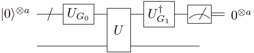
Figure 2: Quantum circuit for block encoding with post-selection on the 0 outcome of the measurements.

Block encoding is in essence a unitary dilation problem, and it is mathematically feasible if and only if $\|A\|\leq 1$. For a general square matrix $A$, we can introduce a normalization factor $\alpha_{A}\geq\|A\|$ and block encode $A/\alpha_{A}$. Without loss of generality, we assume $\|A\|\leq 1$ for the input matrix $A$ in this paper. There are various block encoding constructions based on different input models, including sparse-access matrices, density operators, matrices stored in quantum data structures and so on. We refer the reader to [21, 22] for concrete implementation.

The block encoding framework allows quantum computers to efficiently perform arithmetic operations on matrices. Here we review the method for implementing linear combinations of block encoded matrices, which will be used in subsequent sections. Suppose we have matrices $A_{j}$ block encoded as $(\langle 0|^{\otimes a}\otimes I)U_{j}(|0\rangle^{\otimes a}\otimes I)$ for $j=0,1,\dots,l-1$, and we want to block encode the linear combination $\sum_{j=0}^{l-1}\alpha_{j}A_{j}$ for some coefficients $\alpha_{j}$. Define

$$|G_{0}\rangle=\frac{1}{\sqrt{\sum_{k=0}^{l-1}|\alpha_{k}|}}\sum_{j=0}^{l-1}\sqrt{\alpha_{j}}|j\rangle|0\rangle^{\otimes a},\,|G_{1}\rangle=\frac{1}{\sqrt{\sum_{k=0}^{l-1}|\alpha_{k}|}}\sum_{j=0}^{l-1}\sqrt{\bar{\alpha}_{j}}|j\rangle|0\rangle^{\otimes a},$$ (18)

$$U=\sum_{j=0}^{l-1}|j\rangle\langle j|\otimes U_{j}.$$ (19)

Here $\sqrt{a_{j}}=\sqrt{r_{j}}e^{i\theta_{j}/2}$ for $a_{j}=r_{j}e^{i\theta_{j}}$. Then we have

$$(\langle G_{1}|\otimes I)U(|G_{0}\rangle\otimes I)=\frac{\sum_{j=0}^{l-1}\alpha_{j}A_{j}}{\sum_{k=0}^{l-1}|\alpha_{k}|}.$$ (20)

The construction consists of two parts: a state preparation subroutine (Eq.(18)) that can be implemented using $\Theta(n)$ gates [23], and an operator selection subroutine (Eq.(19)) which can be realized with gate complexity $\Theta(n)$ [24].

Block encoding enhanced with the qubitization technique allows for efficient polynomial transformations to the singular values of a block encoded matrix, the so-called quantum singular value transformation (QSVT). QSVT [21] provides a paradigm that unifies a host of quantum algorithms ranging from quantum simulation to quantum walks. The following lemma is a block encoded version of the quantum linear system solver, which can be realized within the QSVT framework.

Lemma 1 (Inversion of a block encoded matrix [21]).

Let $A$ be a matrix that is block encoded by some unitary $U_{A}$. Then the operator $A^{-1}/\alpha$ can be block encoded with accuracy $\epsilon$ using $O(\kappa\log\frac{1}{\epsilon})$ queries to $U_{A}$ and its inverse, where $\kappa$ is the condition number of $A$.

2.3 Functions of Matrices

There are a number of equivalent ways of defining matrix function $f(A)$ [25] and we give a definition that based on the Jordan canonical form here.

In general, for a complex square matrix $A\in M_{n}(\mathbb{C})$, there is a nonsingular matrix $S\in M_{n}(\mathbb{C})$, positive integers $p$ and $d_{1},\dots,d_{p}$ with $d_{1}+\dots+d_{p}=n$, and scalars $\lambda_{1},\dots,\lambda_{p}\in\mathbb{C}$ such that $A=SJS^{-1}$, where $J=J_{d_{1}}(\lambda_{1})\oplus J_{d_{2}}(\lambda_{2})\oplus\cdots\oplus J_{d_{p}}(\lambda_{p})$ is the Jordan canonical form of $A$ with $J_{d_{i}}(\lambda_{i})$ being

$$J_{d_{i}}(\lambda_{i})=\begin{bmatrix}\lambda_{i}&&&\\ 1&\lambda_{i}&&\\ &\ddots&\ddots&\\ &&1&\lambda_{i}\\ \end{bmatrix}\in\mathbb{C}^{d_{i}\times d_{i}}.$$ (21)

The Jordan matrix $J$ is unique up to the ordering of the blocks $J_{d_{i}}(\lambda_{i})$, while the transforming matrix $S$ is not unique.

A function $f$ is said to be defined on the spectrum of $A$ if for any eigenvalue $\lambda_{i}$ of $A$, $f^{(j)}(\lambda_{i}),j=0,\dots,d_{i}-1$ exist. For such function $f$, the matrix function $f(A)$ is defined as

$$f(A)=Sf(J)S^{-1}=S\begin{bmatrix}f(J_{d_{0}}(\lambda_{0}))&&&\\ &f(J_{d_{1}}(\lambda_{1}))&&\\ &&\ddots\\ &&&f(J_{d_{q}}(\lambda_{q}))\end{bmatrix}S^{-1},$$ (22)

$$f(J_{d_{i}}(\lambda_{i}))=\begin{bmatrix}f(\lambda_{i})&&&&&\\ f^{(1)}(\lambda_{i})&f(\lambda_{i})&&&&\\ \vdots&\ddots&\ddots&&&\\ \vdots&\ddots&\ddots&\ddots&&\\ \frac{f^{(d_{i}-1)(\lambda_{i})}}{(d_{i}-1)!}&\cdots&\cdots&f^{(1)}(\lambda_{i})&f(\lambda_{i})\end{bmatrix}.$$

If $f$ has the Taylor series representation

$$f(z)=\sum_{k=0}^{\infty}\frac{f^{(k)}(z_{0})}{k!}(z-z_{0})^{k},\,|z-z_{0}|<r,$$ (23)

and $|\lambda_{i}-z_{0}|<r$ for every eigenvalue $\lambda_{i}$ of $A$, then there is an equivalent definition [26] via Taylor series:

$$f(A)=\sum_{k=0}^{\infty}\frac{f^{k}(z_{0})}{k!}(A-z_{0}I)^{k}.$$ (24)

3 Polynomial Transformations of a Matrix

In this section, we demonstrate how to implement Chebyshev polynomial transformations and (positive integer) power function transformations of a matrix in the quantum circuit model. We adopt the method of matrix generating function from [17]. Here we take a step further and consider the Chebyshev polynomials defined on the complex plane. Note that Chebyshev polynomial series and integer power function series are two special polynomial series in the context of approximation theory.

3.1 Chebyshev Polynomial Transfromations

The $j$th Chebyshev polynomial of the first kind on the complex plane is defined as

$$T_{j}(z)=\cos(j\arccos(z))=\frac{1}{2}\left[(z+\sqrt{z^{2}-1})^{j}+(z-\sqrt{z^{2}-1})^{j}\right],\,j\geq 0.$$ (25)

From eq.(25) one can easily derive the following recurrence relation

$$T_{j+2}(z)=2zT_{j+1}(z)-T_{j}(z),\,j\geq 0.$$ (26)

Consider the power series $\sum_{j=0}^{\infty}T_{j}(z)y^{j}$ with coefficients $T_{j}(z)$,

$$(1-2zy+y^{2})\sum_{j=0}^{\infty}T_{j}(z)y^{j}$$ (27)

$$= T_{0}(z)+\big{(}T_{1}(z)-2zT_{0}(z)\big{)}y+\sum_{j=2}^{\infty}\big{(}T_{j}(z)-2zT_{j-1}(z)+T_{j-2}(z)\big{)}y^{2}$$

$$= 1-zy.$$

Accordingly, we have the generating function for Chebyshev polynomials

$$\sum_{j=0}^{\infty}T_{j}(z)y^{j}=\frac{1-zy}{1-2zy+y^{2}}.$$ (28)

Similarly, the $j$th Chebyshev polynomial of the second kind is given by

$$U_{j}(z)=\frac{\sin((j+1)\arccos(z))}{\sin(\arccos(z))},$$ (29)

and the corresponding generating function is

$$\sum_{j=0}^{\infty}U_{j}(z)y^{j}=\frac{1}{1-2zy+y^{2}}.$$ (30)

One of the relations between the two kinds of chebyshev polynomials is

$$T_{j}(z)=\frac{1}{2}(U_{j}(z)-U_{j-2}(z))$$ (31)

for $j\geq 2$.

Let $L_{m}=\sum_{k=0}^{m-2}|k+1\rangle\langle k|$ be the $m$-by-$m$ lower shift matrix and $A\in M_{n}(\mathbb{C})$ a matrix with real eigenvalues. Substituting $z=I_{m}\otimes A$ and $y=L_{m}\otimes I_{n}$ in Eq.(28) gives the following matrix version of the generating function

$$\sum_{j=0}^{\infty}L_{m}^{j}\otimes T_{j}(A)=\sum_{j=0}^{m-1}L_{m}^{j}\otimes T_{j}(A) =\begin{bmatrix}T_{0}(A)&&&&\\ T_{1}(A)&T_{0}(A)&&&\\ T_{2}(A)&T_{1}(A)&T_{0}(A)&&\\ \vdots&\ddots&\ddots&\ddots&\\ T_{m-1}(A)&\cdots&T_{2}(A)&T_{1}(A)&T_{0}(A)\end{bmatrix}$$ (32)

$$=\frac{I_{m}\otimes I_{n}-L_{m}\otimes A}{I_{m}\otimes I_{n}+L_{m}^{2}\otimes I_{n}-2L_{m}\otimes A}.$$

The substitution is valid because $L_{m}$ has only one eigenvalue 0, and both sides of Eq.(28) have the same derivatives at $y=0$ of any order. Similarly, the matrix version of the generating function in Eq.(30) is

$$\sum_{j=0}^{\infty}L_{m}^{j}\otimes U_{j}(A)=\sum_{j=0}^{m-1}L_{m}^{j}\otimes U_{j}(A) =\begin{bmatrix}U_{0}(A)&&&&\\ U_{1}(A)&U_{0}(A)&&&\\ U_{2}(A)&U_{1}(A)&U_{0}(A)&&\\ \vdots&\ddots&\ddots&\ddots&\\ U_{m-1}(A)&\cdots&U_{2}(A)&U_{1}(A)&U_{0}(A)\end{bmatrix}$$ (33)

$$=\frac{I_{m}\otimes I_{n}}{I_{m}\otimes I_{n}+L_{m}^{2}\otimes I_{n}-2L_{m}\otimes A}.$$

Our goal is to construct the block encoding of $T_{2^{j}}(A)$. For $j=0$, $T_{2^{j}}(A)$ is simply the matrix $A$. For $j\geq 1$, we set $m=2^{j+1}$ and first block encode the denominator in Eq.(33) $I_{m}\otimes I_{n}+L_{m}^{2}\otimes I_{n}-2L_{m}\otimes A$ with normalization factor 4 (see the construction below), then apply Lemma 1 to implement the block encoding of $(I_{m}\otimes I_{n}+L_{m}^{2}\otimes I_{n}-2L_{m}\otimes A)^{-1}$ (with some normalization factor $\alpha$), which has the matrix representation of Eq.(33). Together with the state preparation (the subscripts of operators $H$ and $X$ indicate the qubit position they are acting on; $C_{m}=\sum_{k=0}^{m-2}|k+1\rangle\langle k|$ is the cyclic shift operator)

$$|G_{0}\rangle=\frac{|m/2-1\rangle-|m/2+1\rangle}{\sqrt{2}}=C_{m}^{m/2-1}H_{(2)}X_{(2)}|0\rangle^{\otimes(j+1)},$$ (34)

and the state unpreparation

$$|G_{1}\rangle=|m-1\rangle=X^{\otimes(j+1)}|0\rangle^{\otimes(j+1)},$$ (35)

we obtain the block encoding

$$\textstyle{\frac{1}{\alpha}}(\langle G_{1}|\otimes I_{n})(I_{m}\otimes I_{n}+L_{m}^{2}\otimes I_{n}-2L_{m}\otimes A)^{-1}(|G_{0}\rangle\otimes I_{n})$$ (36)

$$= \textstyle{\frac{1}{\alpha}}(\langle G_{1}|\otimes I_{n})\Big{(}\textstyle{\frac{1}{\sqrt{2}}}|m/2-1\rangle\otimes U_{0}(A)+\textstyle{\frac{1}{\sqrt{2}}}|m/2\rangle\otimes U_{1}(A)+\textstyle{\frac{1}{\sqrt{2}}}{\sum_{i=1}^{m/2-1}}|m/2+i\rangle\otimes(U_{i+1}(A)-U_{i-1}(A))\Big{)}$$

$$= \textstyle{\frac{1}{\alpha}}(\langle m-1|\otimes I_{n})\Big{(}\textstyle{\frac{1}{\sqrt{2}}}|m/2-1\rangle\otimes U_{0}(A)+\textstyle{\frac{1}{\sqrt{2}}}|m/2\rangle\otimes U_{1}(A)+\sqrt{2}{\sum_{i=1}^{m/2-1}}|m/2+i\rangle\otimes T_{i+1}(A)\Big{)}$$

$$= \textstyle{\frac{\sqrt{2}}{\alpha}}T_{2^{j}}(A).$$

In what follows we demonstrate the block encoding implementation of the operator $I_{m}\otimes I_{n}+L_{m}^{2}\otimes I_{n}-2L_{m}\otimes A$. To block encode the lower shift operator $L_{m}$, consider the $2m$-by-$2m$ cyclic shift operator (a unitary)

$$C_{2m}=\sum_{k=0}^{2m-2}|k+1\rangle\langle k|=\left[\begin{array}[]{ccccc:ccccc}0&&&&&&&&&1\\ 1&0&&&&&&&&\\ &1&0&&&&&&&\\ &&\ddots&\ddots&&&&&&\\ &&&1&0&&&&&\\ \hdashline&&&&1&0&&&&\\ &&&&&1&0&&&\\ &&&&&&1&0&&\\ &&&&&&&\ddots&\ddots&\\ &&&&&&&&1&0\end{array}\right],$$ (37)

where $L_{m}$ appears naturally in the top-left block of $C_{2m}$. Thus we have the following block encoding of $L_{m}$:

$$(\langle 0|\otimes I_{m})C_{2m}(|0\rangle\otimes I_{m})=L_{m}.$$ (38)

Similarly, the block encoding of $L_{m}^{j}$ (for $j=0,1,\dots,m-1)$ is given by

$$(\langle 0|\otimes I_{m})C_{2m}^{j}(|0\rangle\otimes I_{m})=L_{m}^{j}.$$ (39)

Assume $A$ is block encoded as $(\langle 0|^{\otimes a}\otimes I_{n})U_{A}(|0\rangle^{\otimes a}\otimes I_{n})$, then $I_{m}\otimes I_{n}+L_{m}^{2}\otimes I_{n}-2L_{m}\otimes A$ can be implemented via linear combination of block encoded matrices as shown in Section 2.2. To do this, we prepare the state

$$U_{G_{0}}|00\rangle =\big{(}|0\rangle\langle 0|\otimes H+|1\rangle\langle 1|\otimes I\big{)}\big{(}R_{x}(-\textstyle{\frac{\pi}{2}})\otimes I\big{)}|00\rangle$$

$$=\frac{1}{2}|0\rangle|0\rangle+\frac{1}{2}|0\rangle|1\rangle+i\frac{\sqrt{2}}{2}|1\rangle|0\rangle,$$ (40)

$$U_{G_{1}}|00\rangle =\big{(}|0\rangle\langle 0|\otimes H+|1\rangle\langle 1|\otimes I\big{)}\big{(}R_{x}(\textstyle{\frac{\pi}{2}})\otimes I\big{)}|00\rangle$$

$$=\frac{1}{2}|0\rangle|0\rangle+\frac{1}{2}|0\rangle|1\rangle-i\frac{\sqrt{2}}{2}|1\rangle|0\rangle,$$ (41)

and implement the unitary selection

$$|0\rangle\langle 0|\otimes(I_{2}\otimes I_{m}\otimes I_{2^{a}}\otimes I_{n})+|0\rangle\langle 1|\otimes(C_{2m}^{2}\otimes I_{2^{a}}\otimes I_{n})+|1\rangle\langle 0|\otimes(C_{2m}\otimes U_{A}).$$ (42)

Then the circuit in Fig.3 is a block encoding of the operator $\frac{1}{4}(I_{m}\otimes I_{n}+L_{m}^{2}\otimes I_{n}-2L_{m}\otimes A)$.

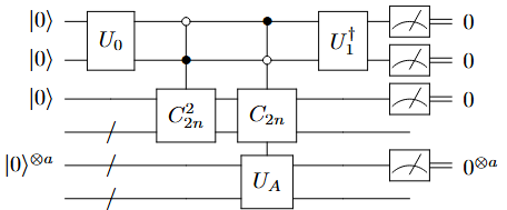
Figure 3: A block encoding of the operator $\frac{1}{4}(I_{m}\otimes I_{n}+L_{m}^{2}\otimes I_{n}-2L_{m}\otimes A)$.

Note that the inverse of a block encoded matrix is only approximately block encoded according to Lemma 1. Assume $\frac{1}{\alpha}(I_{m}\otimes I_{n}+L_{m}^{2}\otimes I_{n}-2L_{m}\otimes A)^{-1}$ is block encoded by unitary $U_{\rm inv_{1}}$ with $\epsilon_{0}$ accuracy

$$\left\|\textstyle{\frac{1}{\alpha}}(I_{m}\otimes I_{n}+L_{m}^{2}\otimes I_{n}-2L_{m}\otimes A)^{-1}-(\langle 0|^{\otimes 3}\otimes I_{m}\otimes\langle 0|^{\otimes a}\otimes I_{n})U_{\rm inv_{1}}(|0\rangle^{\otimes 3}\otimes I_{m}\otimes|0\rangle^{\otimes a}\otimes I_{n})\right\|\leq\epsilon_{0},$$ (43)

then $U_{T_{2^{j}}}=(I_{4}\otimes I_{2}\otimes X^{\otimes(j+1)}\otimes I_{2^{a}}\otimes I_{n})U_{\rm inv_{1}}(I_{4}\otimes I_{2}\otimes C_{m}^{m/2-1}H_{(2)}X_{(2)}\otimes I_{2^{a}}\otimes I_{n})$ is the unitary that block encodes $\frac{\sqrt{2}}{\alpha}T_{2^{j}}(A)$ with $\epsilon_{0}$ accuracy:

$$\left\|\textstyle{\frac{\sqrt{2}}{\alpha}}T_{2^{j}}(A)-(\langle 0|^{\otimes s}\otimes I_{n})U_{T_{2^{j}}}(|0\rangle^{\otimes s}\otimes I_{n})\right\|\leq\epsilon_{0},$$ (44)

where $s=a+j+4$ is number of ancilla qubits. From here we absorb $\sqrt{2}$ into $\alpha$ and simply say that $T_{2^{j}}(A)$ is block encoded with normalization factor $\alpha$ and accuracy $\epsilon_{0}$.

3.2 Power Function Transformation

To deal with matrices with complex eigenvalues, we would need the block encoding of $A^{2^{j}}$. To this end, we consider the generating function for positive integer power functions:

$$\sum_{j=0}^{\infty}z^{j}y^{j}=\frac{1}{1-zy}.$$ (45)

Substituting $y=L_{m}\otimes I_{n}$ and $z=I_{m}\otimes A$ in Eq.(45), we have the matrix generating function for power functions:

$$\sum_{j=0}^{m-1}L_{m}^{j}\otimes A^{j}=\frac{I_{m}\otimes I_{n}}{I_{m}\otimes I_{n}-L_{m}\otimes A}=\begin{bmatrix}I&&&&\\ A&I&&&\\ A^{2}&A&I&&\\ \vdots&\ddots&\ddots&\ddots&\\ A^{m-1}&\cdots&\cdots&A&I\end{bmatrix}$$ (46)

Based on Eq.(46), the block encoding implementation of $A^{2^{j}}$ can be achieved in a similar way as in Section 3.1. It can be directly verified that Fig.4 is a block encoding of the denominator $I_{m}\otimes I_{n}-L_{m}\otimes A$ with normalization factor 2. Next, apply Lemma 1 to construct a unitary $U_{\rm inv_{2}}$ that block encodes $\frac{1}{\alpha}(I_{m}\otimes I_{n}-L_{m}\otimes A)^{-1}$. Then, using the same state preparation Eq.(34) and unpreparation Eq.(35), we obtain the block encoding of $A^{2^{j}}$:

$$\textstyle{\frac{1}{\alpha}}(\langle G_{1}|\otimes I_{n})(I_{m}\otimes I_{n}-L_{m}\otimes A)^{-1}(|G_{0}\rangle\otimes I_{n})=\textstyle{\frac{\sqrt{2}}{\alpha}}A^{2^{j}}.$$ (47)

Let $U_{\rm inv_{2}}$ be the unitary that block encodes $\frac{1}{\alpha}(I_{m}\otimes I_{n}-L_{m}\otimes A)^{-1}$ with $\epsilon_{0}$ accuracy

$$\|\textstyle{\frac{1}{\alpha}}(I_{m}\otimes I_{n}-L_{m}\otimes A)^{-1}-(\langle 0|^{\otimes 2}\otimes I_{m}\otimes\langle 0|^{\otimes a}\otimes I_{n})U_{\rm inv_{2}}(|0\rangle^{\otimes 2}\otimes I_{m}\otimes|0\rangle^{\otimes a}\otimes I_{n})\|\leq\epsilon_{0}$$ (48)

then $U_{A^{2^{j}}}=(X^{\otimes(j+1)}\otimes I_{n})U_{\rm inv_{2}}(C_{n}^{n/2-1}H_{(2)}X_{(2)}\otimes I_{n})$ block encodes $\frac{\sqrt{2}}{\alpha}A^{2^{j}}$ with accuracy $\epsilon_{0}$

$$\left\|\textstyle{\frac{\sqrt{2}}{\alpha}}A^{2^{j}}-(\langle 0|^{\otimes t}\otimes I_{n})U_{A^{2^{j}}}(|0\rangle^{\otimes t}\otimes I_{n})\right\|\leq\epsilon_{0},$$ (49)

where $t=a+j+3$ is the number of ancilla qubits. In the same way, we absorb $\sqrt{2}$ into $\alpha$ and simply say that we have access to a block encoding of $A^{2^{j}}$ with normalization factor $\alpha$.

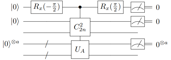
Figure 4: A block encoding of the operator $\frac{1}{2}(I\otimes I-L\otimes A)$.

4 Quantum Eigensolver

In the problem of eigenvalue estimation, we are given a matrix $A$ that satisfies $A|\psi_{\lambda}\rangle=\lambda|\psi_{\lambda}\rangle$. Our goal is to estimate $\lambda$ to some desired precision. Assume we have access to an oracle $U_{A}$ that block encodes $A$ and an input state $|\psi\rangle$ that has sufficient overlap with the eigenstate $|\psi_{\lambda}\rangle$. Specifically,

$$|\psi\rangle=\sqrt{1-\eta}|\psi_{\lambda}\rangle+e^{i\theta}\sqrt{\eta}|\psi_{\perp}\rangle,$$ (50)

where $\langle\psi_{\lambda}|\psi_{\perp}\rangle=0$ and $0\leq\eta\leq\eta_{0}<\frac{1}{2}$, $\eta_{0}$ is a known upper bound for $\eta$. We first tackle the case of real eigenvalues in section 4.1, and deal with complex eigenvalues in section 4.2 by estimating modulus and phase separately.

4.1 Quantum Eigensolver for a Real Eigenvalue

We first rescale the matrix $A$ using the circuit in Fig.5 such that $\|A\|\leq\frac{1}{4}$. Let $\lambda=\cos(2\pi\phi)\in[-\frac{1}{2},\frac{1}{2}]$ be a real eigenvalue of $A$. The expectation of $T_{A^{2^{j}}}$ with respect to the initial state $|\psi\rangle$ is

$$\frac{1}{\alpha}\langle\psi|T_{2^{j}}(A)|\psi\rangle=\frac{1-\eta}{\alpha}\cos(2^{j}\phi\cdot 2\pi)+\frac{\eta}{\alpha}\langle\psi_{\perp}|T_{2^{j}}(A)|\psi_{\perp}\rangle.$$ (51)

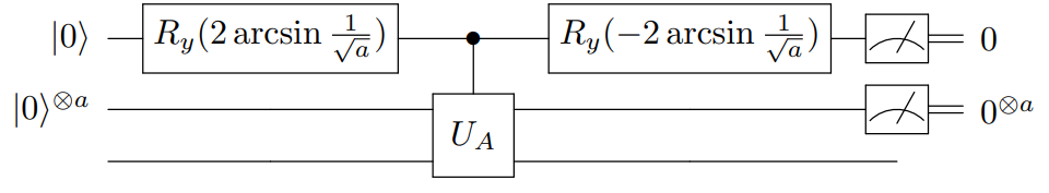
Figure 5: Quantum circuit that rescales $A$ to $\frac{1}{a}A$.

According to section 2.1, running the real and imaginary Hadamard test on $(\langle 0|^{\otimes s}\otimes I_{n})U_{T_{2^{j}}}(|0\rangle^{\otimes s}\otimes I_{n})$ each for $N=\lceil\frac{8}{\delta^{2}}\log_{2}\frac{4}{p_{\text{fail}}}\rceil$ times, we obtain an $\frac{\delta}{2}$-estimation $\bar{Z}_{j}$ of $(\langle 0|^{\otimes s}\langle\psi|)U_{T_{2^{j}}}(|0\rangle^{\otimes s}|\psi\rangle)$ with success probability at least $1-p_{\text{fail}}$. Set $\epsilon_{0}=\frac{\delta}{2}$ in eq.(43), then

$$\left|\bar{Z}_{j}-\frac{1}{\alpha}\langle\psi|T_{2^{j}}(A)|\psi\rangle\right|$$ (52)

$$\leq \left|\bar{Z}_{j}-(\langle 0|^{\otimes s}\langle\psi|)U_{T_{2^{j}}}(|0\rangle^{\otimes s}|\psi\rangle)\right|+\left|(\langle 0|^{\otimes s}\langle\psi|)U_{T_{2^{j}}}(|0\rangle^{\otimes s}|\psi\rangle)-\frac{1}{\alpha}\langle\psi|T_{2^{j}}(A)|\psi\rangle\right|$$

$$\leq \frac{\delta}{2}+\frac{\delta}{2}=\delta.$$

On the other hand, from eq.(51),

$$\left|\bar{Z}_{j}-\frac{1}{\alpha}\langle\psi|T_{2^{j}}(A)|\psi\rangle\right|\geq\left|\bar{Z}_{j}-\frac{1-\eta}{\alpha}\cos(2^{j}\phi\cdot 2\pi)\right|-\frac{\eta_{0}}{\alpha}.$$ (53)

It follows that

$$\left|\bar{Z}_{j}-\frac{1-\eta}{\alpha}\cos(2^{j}\phi\cdot 2\pi)\right|\leq\delta+\frac{\eta_{0}}{\alpha}=R.$$ (54)

The geometric meaning of eq.(54) is that $\bar{Z}_{j}=r_{j}e^{i\theta_{j}}$ lies in the ball $B_{R}\left(\frac{1-\eta}{\alpha}\cos(2^{j}\phi\cdot 2\pi)\right)$ (see Fig.6). Solving this inequality gives

$$r_{j}\cos\theta_{j}-\sqrt{R^{2}-(r_{j}\sin\theta_{j})^{2}}\leq\frac{1-\eta}{\alpha}\cos(2^{j}\phi\cdot 2\pi)\leq r_{j}\cos\theta_{j}+\sqrt{R^{2}-(r_{j}\sin\theta_{j})^{2}}.$$ (55)

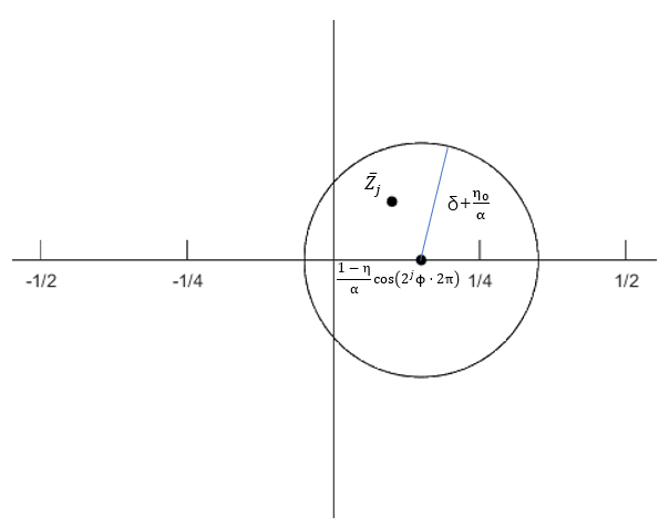
Figure 6: Illustration of eq.(54).

Using the bound $1-\eta_{0}\leq 1-\eta\leq 1$, we have

$$\alpha\left(r_{j}\cos\theta_{j}-\sqrt{R^{2}-(r_{j}\sin\theta_{j})^{2}}\right)\leq\cos(2^{j}\phi\cdot 2\pi)\leq\frac{\alpha}{1-\eta_{0}}\left(r_{j}\cos\theta_{j}+\sqrt{R^{2}-(r_{j}\sin\theta_{j})^{2}}\right).$$ (56)

Under certain conditions (see Theorem 1), the left end point $a_{j}=\alpha\left(r_{j}\cos\theta_{j}-\sqrt{R^{2}-(r_{j}\sin\theta_{j})^{2}}\right)>-1$. We shall use a simpler bound for $\cos(2^{j}\phi\cdot 2\pi)$:

$$a_{j}\leq\cos(2^{j}\phi\cdot 2\pi)\leq 1.$$ (57)

Eq.(57) is equivalent to

$$2^{j}\phi\cdot 2\pi\in[0,\arccos(a_{j})]_{\text{mod}\,2\pi}\cup[2\pi-\arccos(a_{j}),2\pi]_{\text{mod}\,2\pi}.$$ (58)

For the eigenvalue problem we consider here, the two intervals in Eq.(58) are equivalent and we simply say that

$$2^{j}\phi\cdot 2\pi\in\left[0,\arccos(a_{j})\right]_{\text{mod}\,2\pi}.$$ (59)

Algorithm 1 describes the procedure to estimate $\phi$ by narrowing down the interval in eq.(59) iteratively. The following theorem is the correctness proof of Algorithm 1.

Theorem 1.

Let $A$ be a square matrix that satisfies $A|\psi_{\lambda}\rangle=\lambda|\psi_{\lambda}\rangle$ with $\lambda\in\mathbb{R}$. Suppose we have access to an initial state $|\psi\rangle=\sqrt{1-\eta}|\psi_{\lambda}\rangle+e^{i\theta}\sqrt{\eta}|\psi_{\perp}\rangle$ such that $\langle\psi_{\lambda}|\psi_{\perp}\rangle=0$ and $0\leq\eta\leq\eta_{0}<\frac{1}{8}$. Then, Algorithm 1 outputs an estimate of $\lambda$ with arbitrary prescribed precision $\epsilon$ and success probability $1-p_{\rm fail}$.

Proof.

According to Eq.(59), $\phi$ is in one of the intervals

$$I_{k}^{(j)}=\left[\frac{2k\pi}{2^{j}2\pi},\frac{\arccos(a_{j})+2k\pi}{2^{j}2\pi}\right],k=0,1,\dots,2^{j}-1.$$ (60)

We claim that the interval length of each $I_{k}^{(j)}$ is less than the gap length between intervals in $\{I_{k}^{(j+1)},k=0,1,2^{j+1}-1\}$:

$$\frac{\arccos(a_{j})}{2^{j}2\pi}\leq\frac{2\pi-\arccos(a_{j+1})}{2^{j+1}2\pi}.$$ (61)

Rewrite eq.(61) as

$$2\arccos(a_{j})+\arccos(a_{j+1})\leq 2\pi.$$ (62)

Let $\arccos(a_{j_{*}})=\max_{j}\{\arccos(a_{j})\}$, then it suffices to show that $\arccos(a_{j_{*}})\leq\frac{2\pi}{3}$, or equivalently, $a_{j_{*}}\geq-\frac{1}{2}$. This follows by requiring that $\eta_{0}<\frac{1}{8}$ and $\delta\leq\frac{1}{\alpha}(\frac{1}{8}-\eta_{0})$:

$$a_{j_{*}}=\alpha\left(r_{j_{*}}\cos\theta_{j_{*}}-\sqrt{\left(\delta+\frac{\eta_{0}}{\alpha}\right)^{2}-(r_{j_{*}}\sin\theta_{j_{*}})^{2}}\right) >\alpha\left(-\frac{1-\eta}{4\alpha}-2(\delta+\frac{\eta_{0}}{\alpha})\right)$$ (63)

$$=-\frac{1-\eta}{4}-2(\alpha\delta+\eta_{0})$$

$$\geq-\frac{1}{2},$$

where we have use the fact that $r_{j}\cos\theta_{j}\geq\frac{1-\eta}{\alpha}\cos(2^{j}\phi\cdot 2\pi)-(\delta+\frac{\eta_{0}}{\alpha})\geq-\frac{1-\eta}{4\alpha}-(\delta+\frac{\eta_{0}}{\alpha})$.

Eq.(61) means each interval from $\{I_{k}^{(j)},k=0,1,\dots,2^{j}-1\}$ can intersect with at most one of the intervals $I_{k}^{(j+1)}$. At step $j=0$, $\{I_{k}^{(0)},k=0\}$ contains only one interval, which is denoted as $I_{k_{*}}^{(0)}$. At $j+1$ step, we choose THE interval from $\{I_{k}^{j+1}\}$ that intersects with $I_{k_{*}}^{(j)}$ and denote it as $\{I_{k_{*}}^{j+1}\}$. Using the midpoint of interval $I_{k_{*}}^{(j)}$ as an estimation for $\phi$:

$$\phi\approx\phi_{j}=\frac{\arccos{a_{j}}+4k_{*}\pi}{2^{j+1}2\pi}.$$ (64)

At step $j=\lfloor\log_{2}(\epsilon^{-1})\rfloor$, the error of this approximation is at most

$$|\phi-\phi_{j}|\leq\frac{\arccos(a_{j})}{2^{j}2\pi}\leq\frac{1}{2^{j+1}}\leq\epsilon.$$ (65)

As for the success probability, $N=\lceil\frac{8}{\delta}\ln\frac{4(J+1)}{p_{\text{fail}}}\rceil$ samples ensures that

$$P\left(|\bar{Z}_{j}-\langle 0|\langle\psi|U_{T_{2^{j}}}|\psi\rangle|0\rangle|\leq\delta\right)\geq 1-\frac{p_{\rm fail}}{J+1}$$ (66)

for every $j$. Then,

$$P\left(\displaystyle{\bigcap\limits_{j=0}^{J}}\left\{|\bar{Z}_{j}-\langle 0|\langle\psi|U_{T_{2^{j}}}|\psi\rangle|0\rangle|\leq\delta\right\}\right)\geq\left(1-\frac{p_{\rm fail}}{J+1}\right)^{J+1}\geq 1-p_{\rm fail}.$$ (67)

∎

Algorithm 1 Quantum Eigensolver for a Real Eigenvalue (RQE)

0:  Oracle $U_{A}$ that block encodes $A$, initial state $|\psi\rangle$ with noise $\eta_{0}<\frac{1}{8}$, target precision $\epsilon$, an upper bound of the failure probability $p_{\text{fail}}$.

0:  An approximation to $\lambda$.

  $J=\lfloor\log_{2}(\epsilon^{-1})\rfloor$, $\delta=\frac{1}{\alpha}(\frac{1}{8}-\eta_{0})$, $\phi_{-1}=0$.

  for $j=0,1,\cdots,J$ do

   Run the real and imaginary Hadamard test on $(\langle 0|^{\otimes s}\otimes I_{n})U_{T_{2^{j}}}(|0\rangle^{\otimes s}\otimes I_{n})$ each for $N=\lceil\frac{8}{\delta^{2}}\ln\frac{4(J+1)}{p_{\text{fail}}}\rceil$ times to generate $\bar{Z}_{j}=r_{j}e^{i\theta_{j}}$.

   $a_{j}\coloneqq\alpha\left(r_{j}\cos\theta_{j}-\sqrt{R^{2}-(r_{j}\sin\theta_{j})^{2}}\right)$.

   Define a candidate set $S_{j}=\left\{\frac{\arccos(a_{j})+4k\pi}{2^{j+1}2\pi},k=0,1,\dots,2^{j}-1\right\}$.

   $\phi_{j}=\arg\min_{\phi\in S_{j}}|\phi-\phi_{j-1}|$.

  end for

  Return $\cos(2\pi\phi_{J})$.

Remark 1.

It appears that the search space $S_{j}$ is exponentially large as $j$ grows. In fact, if we return at each step not only the minimum $\phi_{j}$ but also the index $k_{j}$ corresponding to the minimum value, then there are only two elements that need to be considered at the next step. Specifically, at step $j=1$, $S_{1}$ consists of two element. The two corresponding intervals $I_{k}^{(1)},k=0,1$ lie in the domain $[0,\pi]$ and $[\pi,2\pi]$ respectively. Suppose $\phi_{1}$ corresponds to $k=k_{1}=1$, then at step $j=2$, we only need to consider the two intervals $I_{k}^{(2)},k=2,3$ that lie within $[\pi,2\pi]$. In general, the two elements to be searched in $S_{j}$ at step $j$ are $k=k_{1}\cdot 2^{j-1}+k_{2}\cdot 2^{j-2}+\cdots+k_{j-1}\cdot 2$ and $k=k_{1}\cdot 2^{j-1}+k_{2}\cdot 2^{j-2}+\cdots+k_{j-1}\cdot 2+1$.

Remark 2.

The requirement for $\eta_{0}$ can be improved by rescaling the norm of $A$ to smaller value. For example, if $\|A\|\leq\frac{1}{8}$, then we only need $\eta_{0}<\frac{3}{16}$ so that eq.(63) holds.

4.2 Quantum Eigensolver for a Complex Eigenvalue

To estimate a complex eigenvalue $\lambda=re^{i\theta}$, our strategy is to first estimate the modulus $r$, then apply a phase estimation algorithm to matrix $\frac{1}{r}A$ to obtain an estimate of the phase $\theta$.

To estimate the modulus, we consider the Hermitian matrices $\frac{A+A^{\dagger}}{2}$ and $\frac{A-A^{\dagger}}{2i}$, the block encoding realization of which is depicted in Fig.7. The expectation of these two matrices with respect to the eigenstate $|\psi_{\lambda}\rangle$ are

$$\left\{\begin{aligned} &\langle\psi_{\lambda}|\frac{A+A^{\dagger}}{2}|\psi_{\lambda}\rangle=r\cos\theta,\\ &\langle\psi_{\lambda}|\frac{A-A^{\dagger}}{2i}|\psi_{\lambda}\rangle=r\sin\theta.\end{aligned}\right.$$ (68)

We note that Algorithm 1 is in essence an algorithm that estimates the expectation value of a matrix with respect to some state, if the expectation is real and bounded by 1. Therefore, we apply Algorithm 1 for matrices $\frac{A+A^{\dagger}}{2}$ and $\frac{A-A^{\dagger}}{2i}$ respectively to obtain estimates of $r\cos\theta$ and $r\sin\theta$, from which we can evaluate the value of $r$.

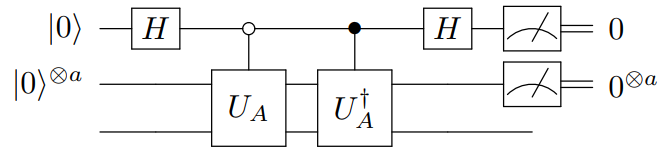
Figure 7: (a)circuit implementation of $\frac{A+A^{\dagger}}{2}$; (b)circuit implementation of $\frac{A-A^{\dagger}}{2i}$.

Next, we block encode a rescaled version $\tilde{A}=\frac{1}{r}A$ of the matrix $A$ using the circuit in Fig.5 and refer to the corresponding unitary as $U_{\tilde{A}}$. We then consider the power function transformations $\tilde{A}^{2^{j}}$, which is block encoded with normalization factor $\alpha$ and accuracy $\epsilon_{0}$ according to Eq.(49):

$$\left\|\frac{1}{\alpha}\tilde{A}^{2^{j}}-(\langle 0|^{\otimes t}\otimes I_{n})U_{\tilde{A}^{2^{j}}}(|0\rangle^{\otimes t}\otimes I_{n})\right\|\leq\epsilon_{0}.$$ (69)

The expectation value of $\tilde{A}^{2^{j}}$ with respect to the initial state $|\psi\rangle$ is

$$\frac{1}{\alpha}\langle\psi|\tilde{A}^{2^{j}}|\psi\rangle=\frac{1-\eta}{\alpha}e^{i2^{j}\theta}+\frac{\eta}{\alpha}\langle\psi_{\perp}|\tilde{A}^{2^{j}}|\psi_{\perp}\rangle.$$ (70)

Running the real and imaginary Hadamard test on $(\langle 0|^{\otimes t}\otimes I_{n})U_{\tilde{A}^{2^{j}}}(|0\rangle^{\otimes t}\otimes I_{n})$ each for $N=\lceil\frac{8}{\delta^{2}}\log_{2}\frac{4}{p_{\text{fail}}}\rceil$ times, we have a $\frac{\delta}{2}$-estimate $\bar{Z}_{j}$ of $(\langle 0|^{\otimes t}\otimes|\psi\rangle)U_{\tilde{A}^{2^{j}}}(|0\rangle^{\otimes t}\otimes|\psi\rangle)$. Combining the error $\epsilon_{0}=\frac{\delta}{2}$ of block encoding gives

$$\left|\bar{Z}_{j}-\frac{1}{\alpha}\langle\psi|\tilde{A}^{2^{j}}|\psi\rangle\right|$$ (71)

$$\leq |\bar{Z}_{j}-(\langle 0|^{\otimes t}\otimes|\psi\rangle)U_{\tilde{A}^{2^{j}}}(|0\rangle^{\otimes t}\otimes|\psi\rangle)|+\left|(\langle 0|^{\otimes t}\otimes|\psi\rangle)U_{\tilde{A}^{2^{j}}}(|0\rangle^{\otimes t}\otimes|\psi\rangle)-\frac{1}{\alpha}\langle\psi|\tilde{A}^{2^{j}}|\psi\rangle\right|$$

$$\leq \delta.$$

On the other hand,

$$\left|\bar{Z}_{j}-\frac{1}{\alpha}\langle\psi|\tilde{A}^{2^{j}}|\psi\rangle\right|\geq\left|\bar{Z}_{j}-\frac{1-\eta}{\alpha}e^{i2^{j}\theta}\right|-\frac{\eta_{0}}{\alpha}.$$ (72)

It follows that

$$\left|\bar{Z}_{j}-\frac{1-\eta}{\alpha}e^{i2^{j}\theta}\right|\leq\delta+\frac{\eta_{0}}{\alpha}\eqqcolon R.$$ (73)

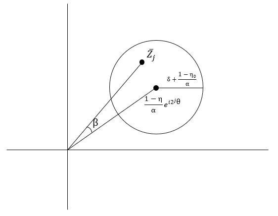
Figure 8: Illustration of eq.(73)

This implies that $\bar{Z}_{j}$ in the ball $B_{R}\left(\frac{1-\eta}{\alpha}e^{i2^{j}\theta}\right)$. Assume $\eta_{0}<2\sqrt{3}-3$ and choose $\delta=\frac{1}{\alpha}\left(\frac{\sqrt{3}}{2}(1-\eta_{0})-\eta_{0}\right)>0$, then the angle $\beta$ (see Fig.8) between $\bar{Z}_{j}$ and the center $\frac{1-\eta}{\alpha}e^{i2^{j}\theta}$ satisfies

$$\sin\beta\leq\frac{\delta+\frac{\eta_{0}}{\alpha}}{\frac{1-\eta}{\alpha}}\leq\frac{\alpha\delta+\eta_{0}}{1-\eta_{0}}=\frac{\sqrt{3}}{2}.$$ (74)

This means that

$$|\arg\bar{Z}_{j}-2^{j}\theta|<\frac{\pi}{3},$$ (75)

or equivalently,

$$2^{j}\theta\in\left(\arg\bar{Z}_{j}-\frac{\pi}{3},\arg\bar{Z}_{j}+\frac{\pi}{3}\right).$$ (76)

The procedure to estimate $\theta$ to some precision based on the above bound is similar to Algorithm 1 and is given in Algorithm 2, which is an adapted version of the robust phase estimation algorithm [11] for unitary matrices. Algorithm 3 describes the estimation process for a complex eigenvalue.

Theorem 2.

Algorithm 3 outputs an estimate for a complex eigenvalue with arbitrary precision $\epsilon$ and success probability $1-p_{\rm fail}$. The algorithm uses $O(\log\frac{1}{\epsilon}\log\frac{1}{p_{\rm fail}})$ queries to $U_{A}$.

Proof.

The error in the estimation of the modulus is upper bounded by

$$|\tilde{r}-r| =|\sqrt{x^{2}+y^{2}}-\sqrt{(r\cos\theta)^{2}+(r\sin\theta)^{2}}|$$ (77)

$$\leq\sqrt{|x^{2}-(r\cos\theta)^{2}+y^{2}-(r\sin\theta)^{2}|}$$

$$\leq\sqrt{|(x-r\cos\theta)+(y-r\sin\theta)|}$$

$$\leq\frac{\epsilon}{2}.$$

Together with the phase estimation error, the error in eigenvalue estimation is

$$\left|\tilde{r}e^{i\tilde{\theta}}-re^{i\theta}\right| =\left|\tilde{r}e^{i\tilde{\theta}}-\tilde{r}e^{i\theta}\right|+\left|\tilde{r}e^{i\theta}-re^{i\theta}\right|$$ (78)

$$\leq\tilde{r}\left|e^{i(\tilde{\theta}-\theta)}-1\right|+\frac{\epsilon}{2}$$

$$\leq 2\tilde{r}\sin\frac{\epsilon}{4\tilde{r}}+\frac{\epsilon}{2}$$

$$\leq\epsilon.$$

The algorithm succeeds only when the three calls to RQE and PES succeed, hence it suffices to require the subroutines to succeed with probability at least $1-\frac{p_{\rm fail}}{3}$.

The construction of $U_{T_{2^{j}}}$ and $U_{A^{2^{j}}}$ each require $O(\kappa\log\frac{1}{\delta})$ queries to $U_{A}$. The computational complexity is dominated by the $O(JN)$ Hadamard tests, hence the query complexity is

$$O\left(\log\frac{1}{\epsilon}\right)\cdot O\left(\frac{1}{\delta^{2}}\ln\frac{4(J+1)}{p_{\rm fail}}\right)\cdot O\left(\kappa\log\frac{1}{\delta}\right)=O\left(\log\frac{1}{\epsilon}\log\frac{1}{p_{\rm fail}}\right).$$ (79)

∎

Algorithm 2 Phase Estimation Subroutine (PES)[11]

0:  Oracle $U_{A}$ that block encodes $A$, initial state $|\psi\rangle$ with noise $\eta_{0}<2\sqrt{3}-3$, target precision $\epsilon$, an upper bound of the failure probability $p_{\text{fail}}$.

0:  An approximation to $\theta$.

  $J=\lfloor\log_{2}(\epsilon^{-1})\rfloor$, $\delta=\frac{1}{\alpha}\left(\frac{\sqrt{3}}{2}(1-\eta_{0})-\eta_{0}\right)$, $\theta_{-1}=0$.

  for $j=0,1,\cdots,J$ do

   Run the real and imaginary Hadamard test on $(\langle 0|^{\otimes t}\otimes I_{n})U_{A^{2^{j}}}(|0\rangle^{\otimes t}\otimes I_{n})$ each for $N=\lceil\frac{8}{\delta^{2}}\log_{2}\frac{4(J+1)}{p_{\text{fail}}}\rceil$ times to generate $\bar{Z}_{j}$.

   Define a candidate set $S_{j}=\left\{\frac{\arg\bar{Z}_{j}+2k\pi}{2^{j}},k=0,1,\dots,2^{j}-1\right\}$.

   $\theta_{j}=\arg\min_{\phi\in S_{j}}|\theta-\theta_{j-1}|$.

  end for

  Return $\theta_{J}$

Algorithm 3 Quantum Eigensolver for a Complex Eigenvalue (CQE)

0:  Oracle $U_{A}$ that block encodes $A$, initial state $|\psi\rangle$ with noise $\eta_{0}<\frac{1}{8}$, target precision $\epsilon$, an upper bound of the failure probability $p_{\text{fail}}$.

0:  An approximation to $\lambda=re^{i\theta}$.

  $x={\rm RQE}\left(\frac{A+A^{\dagger}}{2},|\psi\rangle,\frac{\epsilon^{2}}{8},\frac{p_{\rm fail}}{3}\right)$.

  $y={\rm RQE}\left(\frac{A-A^{\dagger}}{2i},|\psi\rangle,\frac{\epsilon^{2}}{8},\frac{p_{\rm fail}}{3}\right)$.

  $\tilde{r}\coloneqq\sqrt{x^{2}+y^{2}}$.

  $\tilde{\theta}={\rm PES}\left(\frac{1}{\tilde{r}}A,|\psi\rangle,\frac{\epsilon}{2\tilde{r}},\frac{p_{\rm fail}}{3}\right)$.

  Return $\tilde{\lambda}=\tilde{r}e^{i\tilde{\theta}}$.

5 Conclusion

This work provides a simple and efficient quantum eigensolver for general square matrices. The algorithm employs Hadamard test on matrix transformations to generate data that contains the information of the eigenvalue, and then retrieve the information through simple classical postprocessing. In particular, we tackle the case of complex eigenvalues by resolving the problem into modulus estimation and phase estimation. To estimate the modulus or a real eigenvalue, we essentially devise an algorithm that estimates real expectation values of the matrix with respect to some state. The complexity of our algorithm exhibits logarithmic dependence on precision and failure probability, and independence on the matrix side. Hence, our work beats all the existing algorithms, which have undesired complexity scaling of some of the parameters.

References

- [1] László Lovász. Random walks on graphs. Combinatorics, Paul erdos is eighty, 2(1-46):4, 1993.
- [2] Lloyd N Trefethen and David Bau. Numerical linear algebra. SIAM, 2022.
- [3] Heinz-Peter Breuer and Francesco Petruccione. The theory of open quantum systems. Oxford University Press, USA, 2002.
- [4] A. Guo, G. J. Salamo, D. Duchesne, R. Morandotti, M. Volatier-Ravat, V. Aimez, G. A. Siviloglou, and D. N. Christodoulides. Observation of -symmetry breaking in complex optical potentials. Phys. Rev. Lett., 103:093902, Aug 2009.
- [5] Xiujuan Zhang, Tian Zhang, Ming-Hui Lu, and Yan-Feng Chen. A review on non-hermitian skin effect. Advances in Physics: X, 7(1):2109431, 2022.
- [6] Zhiyan Ding and Lin Lin. Even shorter quantum circuit for phase estimation on early fault-tolerant quantum computers with applications to ground-state energy estimation. PRX Quantum, 4:020331, May 2023.
- [7] Zhiyan Ding, Haoya Li, Lin Lin, HongKang Ni, Lexing Ying, and Ruizhe Zhang. Quantum Multiple Eigenvalue Gaussian filtered Search: an efficient and versatile quantum phase estimation method. Quantum, 8:1487, October 2024.
- [8] Dorit Aharonov, Daniel Gottesman, Sandy Irani, and Julia Kempe. The power of quantum systems on a line. In 48th Annual IEEE Symposium on Foundations of Computer Science (FOCS’07), pages 373–383, 2007.
- [9] Guang Hao Low and Isaac L Chuang. Hamiltonian simulation by qubitization. Quantum, 3:163, 2019.
- [10] Shantanav Chakraborty, András Gilyén, and Stacey Jeffery. The Power of Block-Encoded Matrix Powers: Improved Regression Techniques via Faster Hamiltonian Simulation. In Christel Baier, Ioannis Chatzigiannakis, Paola Flocchini, and Stefano Leonardi, editors, 46th International Colloquium on Automata, Languages, and Programming (ICALP 2019), volume 132 of Leibniz International Proceedings in Informatics (LIPIcs), pages 33:1–33:14, Dagstuhl, Germany, 2019. Schloss Dagstuhl – Leibniz-Zentrum für Informatik.
- [11] Hongkang Ni, Haoya Li, and Lexing Ying. On low-depth algorithms for quantum phase estimation. Quantum, 7:1165, 2023.
- [12] Hefeng Wang, Lian-Ao Wu, Yu-xi Liu, and Franco Nori. Measurement-based quantum phase estimation algorithm for finding eigenvalues of non-unitary matrices. Physical Review A—Atomic, Molecular, and Optical Physics, 82(6):062303, 2010.
- [13] Anmer Daskin, Ananth Grama, and Sabre Kais. A universal quantum circuit scheme for finding complex eigenvalues. Quantum information processing, 13:333–353, 2014.
- [14] Changpeng Shao. Computing eigenvalues of diagonalizable matrices on a quantum computer. ACM Transactions on Quantum Computing, 3(4):1–20, 2022.
- [15] Yuta Mizuno and Tamiki Komatsuzaki. Quantum algorithm for dynamic mode decomposition integrated with a quantum differential equation solver. Physical Review Research, 6(4):043031, 2024.
- [16] Xiao-Ming Zhang, Yukun Zhang, Wenhao He, and Xiao Yuan. Exponential quantum advantages for practical non-hermitian eigenproblems, 2024.
- [17] Guang Hao Low and Yuan Su. Quantum eigenvalue processing. arXiv preprint arXiv:2401.06240, 2024.
- [18] Huanfeng Zhao, Peng Zhang, and Tzu-Chieh Wei. A universal variational quantum eigensolver for non-hermitian systems. Scientific Reports, 13(1):22313, 2023.
- [19] Alexander Teplukhin, Brian K. Kendrick, and Dmitri Babikov. Solving complex eigenvalue problems on a quantum annealer with applications to quantum scattering resonances. Phys. Chem. Chem. Phys., 22:26136–26144, 2020.
- [20] Wassily Hoeffding. Probability inequalities for sums of bounded random variables. Journal of the American Statistical Association, 58(301):13–30, 1963.
- [21] András Gilyén, Yuan Su, Guang Hao Low, and Nathan Wiebe. Quantum singular value transformation and beyond: exponential improvements for quantum matrix arithmetics. In Proceedings of the 51st Annual ACM SIGACT Symposium on Theory of Computing, pages 193–204, 2019.
- [22] Lin Lin. Lecture notes on quantum algorithms for scientific computation, 2022.
- [23] Vivek V Shende, Stephen S Bullock, and Igor L Markov. Synthesis of quantum logic circuits. In Proceedings of the 2005 Asia and South Pacific Design Automation Conference, pages 272–275, 2005.
- [24] Andrew M Childs, Dmitri Maslov, Yunseong Nam, Neil J Ross, and Yuan Su. Toward the first quantum simulation with quantum speedup. Proceedings of the National Academy of Sciences, 115(38):9456–9461, 2018.
- [25] NJ Higham. Functions of matrices: Theory and computation, 2008.
- [26] Gene H Golub and Charles F Van Loan. Matrix computations. JHU press, 2013.