Investigating Pulsating Variables and Eclipsing Binaries in NGC 2126 using Ground and Space-based Photometry, Astrometry, Spectroscopy and Modeling

Abstract

Pulsating variables are prevalent in the classical $\delta$ Scuti instability strip of intermediate-age open star clusters. The cluster membership of these stars facilitates a comparative analysis of their evolution in analogous environments. In this study, we integrate ground-based observations, TESS Full Frame Images (FFIs), and Gaia DR3 data to investigate variable stars in the intermediate-age open star cluster NGC 2126. We performed ground-based time-series observations of NGC 2126 to identify variable stars within its vicinity. Next, we determined the membership of these stars using parallax and the proper motions from Gaia DR3 archive. Then, we searched the TESS Full Frame Images (FFIs) for counterparts to the variables identified above and performed their frequency analysis and classification. Finally, we modeled the light curves (LCs) of detected eclipsing binaries (EBs), including V551 Aur, which has a pulsating component. We found 25 members and 85 field variable stars. In TESS FFIs, we found LCs for 11 known variables and a new rotational variable. We determined that the pulsating EB V551 Aur is a member of the cluster. The low- and medium-resolution spectra revealed the line profile variation and the basic parameters for the star, respectively. Simultaneous modeling of the eclipses and the embedded pulsations resulted in improved orbital parameters for the binary system. We also report the determination of orbital parameters for the previously uncharacterized EB system UCAC4 700-043174.

1 INTRODUCTION

Open star clusters comprise stars that have emerged from a common molecular cloud and are gravitationally bound to one another. Consequently, they possess analogous ages, distances, and initial chemical compositions. The membership of stars within an open cluster imposes constraints, especially regarding their age in comparison to the ambiguously determined ages of field stars. Thus, examining stars that are constituents of an open cluster is more advantageous than analyzing field stars. Diverse independent methodologies for stellar characterization, such as asteroseismology (Aerts, 2021), can gain from open clusters by imposing supplementary constraints on parameters like age and mass (Li et al., 2024; Bedding et al., 2023; Pamos Ortega et al., 2023). The intermediate-age open star clusters possess their turn-off point adjacent to the classical instability strip, thereby hosting a variety of pulsating variable stars of A- and F-type, including $\delta$ Scuti stars and $\gamma$ Doradus stars (Chehlaeh et al., 2018).

Ground-based studies of open clusters yield ensemble photometry for a collection of stars within a defined area. The Aryabhatta Research Institute of Observational Sciences (ARIES) in Nainital, India, possesses photometric observational facilities in the northern hemisphere, that are very suitable for studying open clusters. Details regarding the telescopes at the site will be presented in Section 3 later in this paper. To capitalize on the advantages of studying open clusters, ARIES, Nainital is conducting long-term photometric monitoring using 1-meter class telescopes to examine pulsating variable stars in both young open clusters (Joshi et al., 2020a; Lata et al., 2023) and intermediate-age open clusters (Joshi et al., 2020b; Maurya et al., 2023). Additionally, we also performs long-term surveys for pulsating A- and F-type field stars (Ashoka et al., 2000; Martinez et al., 2001; Joshi et al., 2003; Joshi et al., 2006, 2009, 2010; Joshi et al., 2012, 2016b; Joshi et al., 2017). We have recently augmented this exploration with space-based observations from K2 and TESS concerning field stars (Joshi et al., 2022b; Trust et al., 2021, 2023; Sarkar et al., 2024; Dileep et al., 2024). In this study, we integrate the space-based observations for open star clusters with the ground-based observations.

Similar to open star clusters, eclipsing binaries provide an independent assessment of fundamental stellar parameters. They provide accurate measurements of stellar masses and radii through orbital dynamics and eclipse depths (Panchal et al., 2023). If one of the binary components is pulsating, the target becomes increasingly unusual. The examination of pulsations in eclipsing binary (EB) components provides insights into the internal structure of the pulsating star, system evolution, and the influence of tidal forces inducing oscillations (Pigulski, 2006; Murphy, 2019; Lampens, 2021). The existence of these unusual variable systems in open clusters serves as valuable test beds for validating various theoretical models for pulsation and stellar evolution.

We conducted a comprehensive ground- and space-based investigation of the intermediate-age open star cluster NGC 2126 (Gáspár et al., 2003). We utilized ground-based photometric observations from telescopes of varying diameters at ARIES, Nainital, low- to medium-resolution spectra, TESS Full Frame Images (FFIs), and Gaia DR3 data.

The manuscript is structured as follows. Sec. 2 delineates the sample selection, while Sec. 3 examines ground-based observations for the detection of variable stars. In Sec. 4, we ascertain the membership of the detected variables within the cluster, and in Sec. 5, we evaluate the cluster parameters. Subsequently, in Sec. 6, we examine the TESS light curves for all stars and categorize the identified variables in Sec. 7. Ultimately, we present the modeling of the binary LCs in Sec. 8 and provide a summary of our findings in Sec. 9. We present our conclusions in Sec. 10.

2 SAMPLE SELECTION

We selected NGC 2126 (RA = $06^{h}02^{m}37.9^{s}$, Dec = $+49^{o}52^{\prime}59^{\prime\prime}$), which is an intermediate-age open star cluster hosting various pulsating stars located in the $\delta$ Scuti instability strip. The first CCD photometric study of the cluster was performed by Gáspár et al. (2003). Later, it was studied by Liu et al. (2012) and more recently Chehlaeh et al. (2018) presented new ground-based photometric observations for NGC 2126 and reported 11 variables, including two new $\delta$ Scuti variables. This makes this cluster as a potential target for asteroseismic investigation of pulsating variables of A- and F- type. Another reason that makes this cluster interesting is the presence of the EB V551 Aur, which shows pulsational variability on top of the eclipses. The membership of this star to the cluster will place strong constraints on its evolution and pulsation mechanism. All of the previous ground-based studies had limitations due to their short and discrete observations. Thus, aliasing and frequency resolution limit the accuracy of detected frequencies. Furthermore, NGC 2126 has one EB, UCAC4 700-043174, but there was insufficient data to model the system or report an orbital period (Chehlaeh et al., 2018). Thanks to the nearly continuous TESS observations spanning approximately a month in each sectors, we can address the limitations due to lack of continuous data in ground-based observations. The long and short cadence of TESS enables us to study both faint and bright targets of the cluster.

3 GROUND-BASED PHOTOMETRIC OBSERVATIONS

Time-series photometric observations for NGC 2126 were acquired in the $V$ and $R$ bands with the 1.3-m Devasthal Fast Optical Telescope (DFOT), Nainital, India (Joshi et al., 2022a). This telescope is equipped with a 2k $\times$ 2k CCD, gives a field of view of about 18 x 18 arcmin² with a plate scale of 0.54 arcsec/pixel. For standardization of our targets, the standard field SA 98 of Landolt (1992) was also observed in UBVRI filters. For the pre-processing of the images, several bias frames and twilight flats were taken during the observing nights. We furthermore observed the cluster in the V and R bands during one more night using the 1.04-m Sampurnanand Telescope (ST), Nainital, India. This telescope is equipped with a 4k $\times$ 4k CCD, which gives a field of view of about 15 x 15 arcmin² (Yadav et al., 2022). The CCD was used in 4 $\times$ 4 binning mode to increase the signal-to-noise ratio, this gives a plate scale of 0.92 arcsec/pixel after binning. Additionally, we also observed the pulsating EB V551 Aur in NGC 2126 for a couple of nights with the 3.6-m Devasthal Optical Telescope (DOT) (Kumar et al., 2018). This telescope is equipped with a 4k $\times$ 4k CCD Imager that covers a field of view of 6.5 x 6.5 arcmin² (Pandey et al., 2018) and has a plate scale of 0.2 arcsec/pixel after 2 $\times$ 2 binning. An overview with the details of the collected ground-based observations is given in Table 1.

The images were pre-processed with Image Reduction and Analysis Facility (IRAF) tasks: zerocombine, flatcombine, and CCDPROC. We applied the method of point-spread function (PSF) photometry to obtain the instrumental magnitudes for the stars in the target field, for this, we used the code DAOPHOTII by Stetson (1992).

The standard field SA 98 was used to convert the instrumental magnitudes to standard magnitudes. The following equations define the resulting transformations (Stetson, 1987):

$$v=V+(2.064\pm 0.005)+(0.071\pm 0.005)(V-I)+0.21Q$$ (1)

$$b=B+(2.652\pm 0.007)-(0.143\pm 0.006)(B-V)+0.32Q$$ (2)

$$i=I+(2.446\pm 0.008)-(0.036\pm 0.007)(V-I)+0.08Q$$ (3)

$$r=R+(1.910\pm 0.010)+(0.088\pm 0.016)(V-R)+0.13Q$$ (4)

$$u=U+(4.641\pm 0.010)-(0.090\pm 0.011)(U-B)+0.49Q$$ (5)

where v, b, i, r, u are the instrumental magnitudes, and $V,B,I,R,U$ refer to the standard magnitudes and $Q$ is the airmass.

Table 1: Observational log for NGC 2126. The telescopes used for multi-band photometric observations and the date of observations are listed. Each of the columns named $V,R,U,B$ and $I$ have entries of the form ‘number of frames $\times$ exposure time’.

Telescope	Date of	$V$	$R$	$U$	$B$	$I$
	Observation
1.04-m ST	2023 Nov 22	$119\times 50$s	$119\times 50$s	-	-	-
1.3-m DFOT	2022 Oct 29	$71\times 40$s	$70\times 30$s	-	-	-
	2022 Oct 30	$12\times 40$s	$12\times 30$s	-	-	-
	2022 Nov 11	$200\times 50$s	-	-	-	-
	2023 Feb 11	$59\times 50$s	$59\times 30$s	-	-	-
	2023 Feb 14	$44\times 50$s	$44\times 30$s	-	-	-
	2023 Feb 18	$103\times 50$s	$103\times 30$s	-	-	-
	2023 Feb 19	$17\times 50$s	$17\times 30$s	-	-	-
	2023 Oct 15	$50\times 50$s	$3\times 50$s	-	-	-
	2023 Nov 14	$100\times 50$s	$100\times 30$s	-	-	-
	2023 Nov 18	$111\times 50$s	$111\times 50$s	-	-	-
	2023 Dec 02	$102\times 50$s	$103\times 30$s	$3\times 300$s	$3\times 12$0s	$3\times 20$s
3.6-m DOT	2021 Dec 13	$12\times 300$s	-	-	$11\times 100$s	-
		-	-	-	$1\times 150$s	-
	2021 Dec 14	$12\times 100$s	-	-	$9\times 200$s	-
		$10\times 150$s	-	-	$12\times 300$s	-
		$1\times 300$s	-	-	-	-
	2021 Dec 15	$16\times 100$s	-	-	$11\times 270$s	-
		$11\times 80$s	-	-	$12\times 160$s	-
	2023 Mar 28	$50\times 50$s	-	-	-	-

The search for variables in the cluster field was done based on the LCs obtained with 1.3-m DFOT. The $V$-band photometric LCs from each night were combined together and then phase-folded with the period that matches the first main peak in the Lomb-Scargle periodogram. The same period was used to phase-fold the combined $R$-band LCs to see any corresponding variations in the $R$-band. The stars that showed brightness variation greater than three standard deviations with respect to the mean brightness, at least in the $V$-band were considered to be variable stars and were chosen for further analysis. The LCs for newly detected member variables from the ground are given in Fig. 1 and the field stars in Appendix Fig. 26-30. We also list the detected dominant freqeuncies and the corresponding amplitudes of the field stars in Table 8.

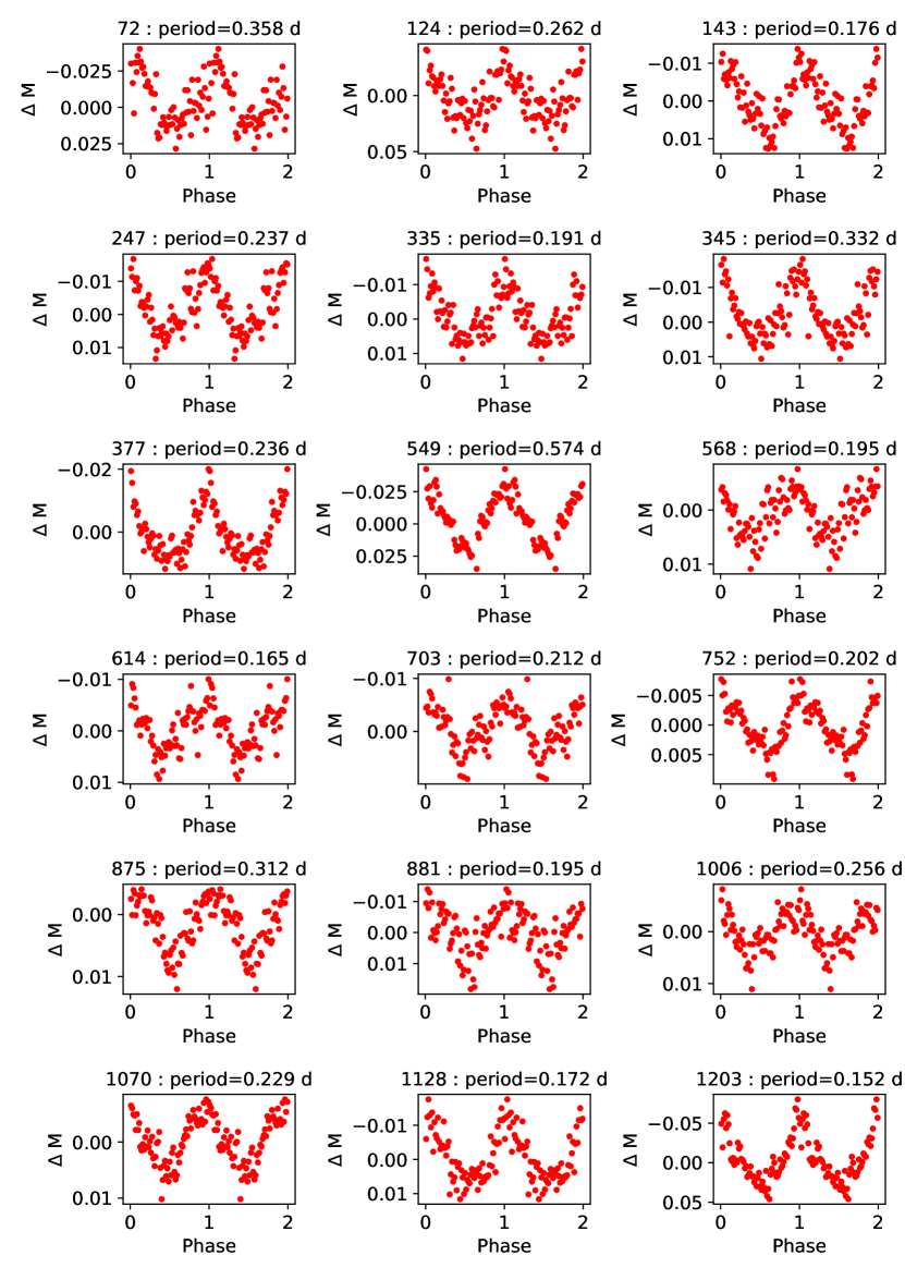
Figure 1: Phase-folded LCs of the newly detected variables, which are the members of open cluster NGC 2126. Their respective IDs and detected periods are given in the title of each plot.

4 CLUSTER MEMBERSHIP

For the determination of membership, we used astrometric data from Gaia DR3. The Gaia mission (Gaia Collaboration et al., 2016) is an all-sky survey that collects multi-band photometric, astrometric, and spectroscopic data. Gaia’s astrometric data have proven to be very successful in identifying and determining the membership of open clusters and globular clusters. The proper motion and parallax of all stars within a radius of 18 arcminutes around the cluster center were obtained by querying the Gaia DR3 catalogue (Gaia Collaboration et al., 2023). Stars with large error bars were excluded from our study. We constructed the vector point diagram (VPD) of the cluster region to identify stars with similar proper motion (Fig. 2). Furthermore, we used the parallaxes to select samples with similar distances. For the membership probability, we used the method described in Wu et al. (2002) by identifying a cluster population and field population from the VPD. For this purpose, we plotted the radial density profile (RDP) of the VPD by calculating the number density in concentric annular regions from the center of the VPD. For the center of VPD, we smoothed the proper motion space with a 2D Gaussian kernel and chose the point with the maximum kernal density. The resultant RDP is shown in Fig. 3 along with a fitted King’s profile (King, 1962). The number density was seen to approach the background density at a radial distance $\sim$ 0.8 mas/yr. We chose this as the limiting radius for probable cluster members and the stars outside this radius as field stars.

The Gaia Color-Magnitude Diagram (CMD) for stars having membership probability greater than 50 % is shown in Fig. 4. The members that are highly probable are situated along the main sequence, the evolved red giant branch, and the turn-off point. These members will introduce substantial constraints on the system’s age by means of isochrone fitting (see Sec. 5).

Figure 2: Top panel shows the vector point diagram of NGC 2126 using Gaia DR3 proper motion data. The Bottom panel shows the position of the cluster members and field stars in the sky as observed by Gaia DR3. Both panels have stars within an 18 arcmins radius from the center which was selected for membership determination. In both panels red dots represents the member stars for which the membership probability is greater than 50 % and gray dots represents the field stars.

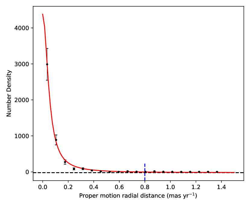
Figure 3: Number density plot for the proper motion space from Gaia data. The red curve shows the best fitting RDP. The black horizontal dashed line shows the background density. The blue vertical dashed line marks the chosen limiting radius.

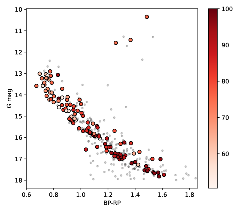
Figure 4: The CMD of NGC 2126 with the field stars (grey dots) and the member stars (color-coded dots according to their calculated membership probability). The probability scale is represented by the color bar on the right side (50 - 100 %).

5 CLUSTER PARAMETERS

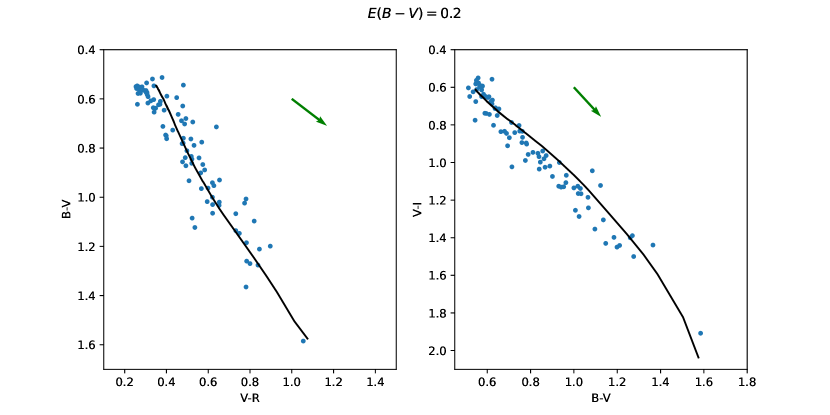
Figure 31: Left panel : The V-R vs B-V diagram for NGC 2126 member stars. Right panel : The B-V vs V-I diagram for NGC 2126 member stars. The black lines in the plot are the theoretical isochrones and the green arrow represents the reddening vector.

The CMD can be used to fit theoretical isochrones and determine cluster parameters such as age, metallicity, and reddening. The age and metallicity of the member stars should be comparable as a result of their shared origin. Thus, by comparing theoretical isochrones of varying ages and metallicities, we can estimate the cluster parameters. The Gaia CMD consists of the BP-RP color and the G-band mean magnitude. We used the isochrones downloaded from the CMD service CMD 3.7 in the Gaia EDR3 photometric system, and the evolutionary tracks from the PARSEC release v1.2S (Bressan et al., 2012; Chen et al., 2014, 2015; Tang et al., 2014). We utilized the Gaia DR3 parallaxes for the cluster members to determine an initial distance modulus and used prior literature values for an initial value for reddening. Utilizing these corrections, we drew a series of isochrones next to the observed CMD. Subsequently, the fit was optimized using the ASteCA code (Perren et al., 2015) by selecting the above guessed range of values (metallicity = [0.010 , 0.030], log age = [9.0 , 9.3], distance modulus = [9, 12], extinction = [0.2, 1] ) as uniform priors. ASteCA computes synthetic isochrones between the given grid of isochrones and uses a genetic algorithm (Charbonneau, 1995) to minimize the negative log likelihood, -log[$L_{i}$(z,a,d,e)], where z is the metallicity, a is the age, d is the distance, and e is the extinction. The genetic algorithm (GA) is an optimization technique derived from natural selection, wherein a population of candidate solutions evolves over generations through selection (optimal fit), crossover (various combinations of parent sets), and mutation (random alterations introduced at each stage) to identify the most effective solution for a specific problem. It is particularly effective in exploring complex, multi-dimensional spaces and avoiding local minima. For more thorough details regarding the algorithm please refer to (Charbonneau, 1995). Additionally to quantify parameter uncertainties we employed the Markov Chain Monte Carlo (MCMC) method within ASteCA, the resultant posterior distribution is shown in Fig. 5. By fitting a Gaussian to the parallax histogram (Fig. 6), we calculated the mean parallax, which allowed us to calculate the distance to the cluster, which came out to be 1.3 $\pm$ 0.1 kpc. Also, we calculated distance to the cluster from the distance modulus of the isochrone fit using standard relations. We used the best fit coefficients published by Gaia team based on the empirical relation used by Danielski et al. (2018) to convert extinction in gaia G-band ($A_{G}$) to extinction in V-band ($A_{V}$), and used $R_{v}$=3.1 to get the reddening $E(B-V)$ for the cluster. We also verified this estimate using color-color diagrams from ground-based observations (Fig. 31). Apart from that a medium-resolution spectrum (see Sec. 8.2) of a member variable, V551 Aur, was used to estimate the reddening towards the cluster. We used the calibration published by Poznanski et al. (2012), between the equivalent width of Na doublets and the reddening (Fig. 7). The final values for the HR diagram were found by taking the average of the distance estimates from the isochrone fit and the parallax fit, as well as the reddening estimates from the isochrone fit and the Na doublets. The best-fit parameters for the cluster are tabulated in Table 2 and the best fit isochrone is plotted in Fig. 8.

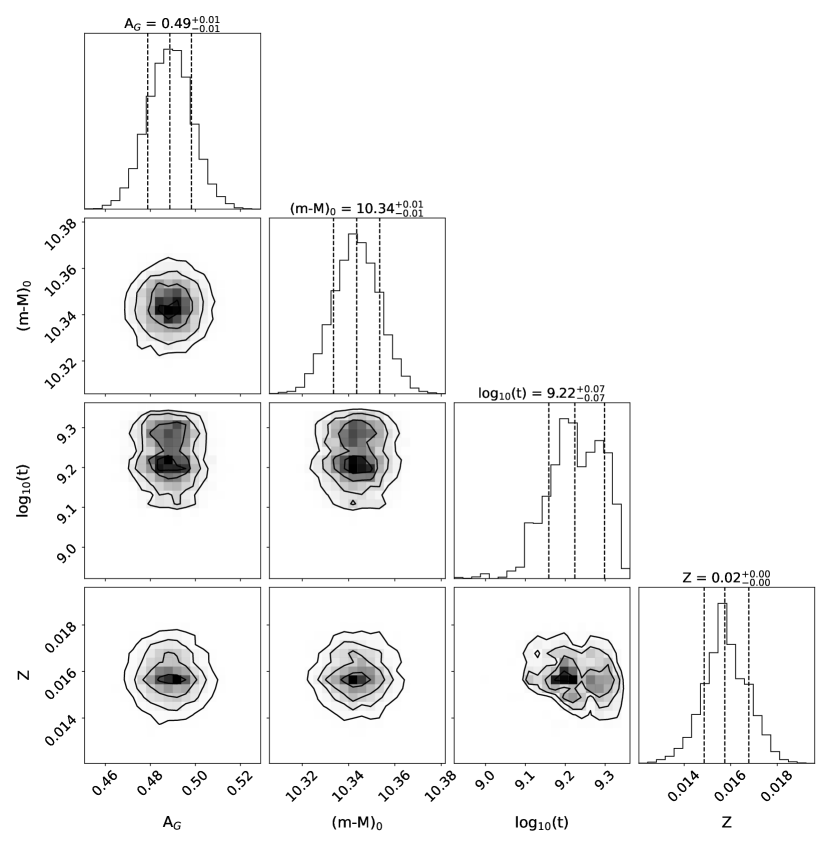
Figure 5: The resultant posterior distribution for the best fit isochrone.

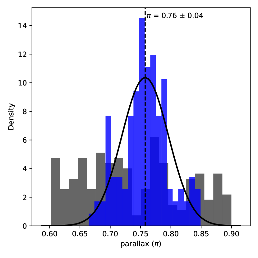
Figure 6: The histogram in blue displays the parallax distribution of the cluster members and the histogram in grey shows the parallax distribution of the field stars. By fitting a Gaussian to the cluster member parallaxes, we obtained the mean cluster parallax, which was then used to determine the distance to the cluster.

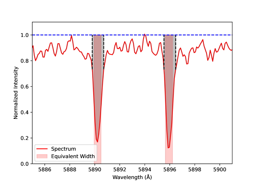
Figure 7: The interstellar absorption lines of Sodium in the medium-resolution spectrum of V551 Aur. The blue horizontal dashed line is the continuum. We selected the regions between the black dashed lines to calculate the equivalent width of Na D1 & D2 lines, filled with gray color in the figure. The resultant equivalent width is the horizontal width of the rectangles drawn between 0 and 1 filled with red color.

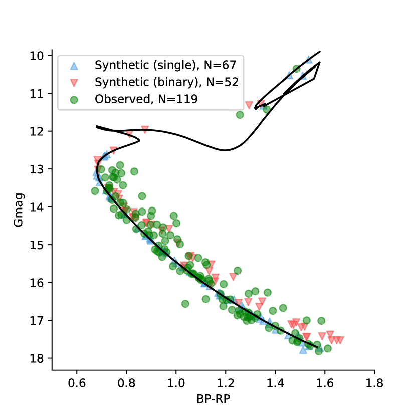
Figure 8: The figure shows the best-fit isochrone using the code ASteCA represented by the black curve. The synthetic members calculated by ASteCA are represented with blue straight and red inverted triangles, respectively. And our input observed members from Gaia DR3 are represented as green circles.

Table 2: The table gives the best-fit parameters for isochrone fitting with ASteCA. Here, Z is the metal fraction, t is the age in years, A_G is the extinction in Gaia G band, $(m-M)_{0}$ is the distance modulus of the cluster, D gives the distance to the cluster and E(B-V) is the reddening. The uncertainty in the last digit is given in brackets for each values.

Parameter	Isochrone fit	Parallax Fit	Na D lines
$log_{10}(t)$	9.22(7)	-	-
$Z$	0.016(1)	-	-
$A_{G}$	0.49(1) mag	-	-
$(m-M)_{0}$	10.34(1) mag	-	-
$D$	1.169(5) kpc	1.3(1) kpc	-
$E(B-V)$	0.20(4)	-	0.29(8)

6 TESS PHOTOMETRY

The Transiting Exoplanet Survey Satellite (TESS) is an all-sky survey telescope whose prime objective is to detect exoplanets orbiting nearby bright stars using the transit method (Ricker, 2014). Apart from its primary mission, it also provides time-series photometry for asteroseismic studies of stars with magnitudes up to 12. TESS Target Pixel Files (TPF) and Light Curve Files are available with short cadences (20 s and 120 s) while Full Frame Images (FFIs) are taken with a longer cadence (30 min). Recently, the FFIs were taken at a shorter cadence of 200 seconds, which we used in our study. These data products can be downloaded from Mikulski Archive for Space Telescopes (MAST).

Given the large pixel size of the TESS CCD, which is 21^′′ per pixel, resolving crowded fields like we see in open star clusters will be difficult, so our search for variability was primarily based on ground-based observations. The higher spatial resolution of ground-based observations enables the resolution of individual stars in the crowded field. Consequently, we concentrated our investigation of variability in the TESS FFIs on sources that had confirmed variable signals from the ground.

TESS observed the field of NGC 2126 during Sector 19 with an 1800-s cadence and during Sectors 59, 60, and 73 with a 200-s cadence. The observations from sector 60 were excluded from this study because the targets were too close to the edge of the TESS CCD, preventing useful photometry. The log of observations taken from the TESS archive is given in Table. 3. We performed the FFI photometry of our targets in the field using the python packages Eleanor (Feinstein et al., 2019) and Lightkurve (Lightkurve Collaboration et al., 2018). To perform the photometry, we relied on the cut-outs taken from the FFI using the package tesscut (Brasseur et al., 2019).

Table 3: NGC 2126 was observed in the sectors listed below. The observation period, cadence (in seconds), and duration (in days) are also given.

TESS	Observation Period	Cadence	Duration
Sector		(s)	(days)
19	28 Nov - 23 Dec, 2019	1800	24.5
59	26 Nov - 23 Dec, 2022	200	26.4
73	07 Dec - 03 Jan, 2024	200	26.9

Eleanor is a Python package that automates the extraction of LCs from FFIs. For sector 19, the Eleanor package was used and the resulting sky-subtracted LCs were free of telescope systematic and suitable for analysis. To identify our targets in the FFI, we overplotted the Gaia sources in the field and the apertures were carefully selected to reduce the contamination from nearby targets. Eleanor did not perform well in sectors 59 and 73, necessitating a manual approach utilizing the Lightkurve package. Here, we also conducted an investigation into the FFI by overplotting the Gaia sources to minimize contamination from nearby sources and used custom apertures to extract the sky-subtracted LCs. As a final step, we used the RegressionCorrector in Lightkurve package. The task creates a design matrix, which is a matrix of flux time series of the background pixels. For which a principal component analysis (PCA) (Deb & Singh, 2009) is performed to reduce its dimensionality and select the first few principal components, which contain most of the instrumental and systematic effects in that particular part of the sector. Then a linear combination of these components is used to remove the long term trends in the light curve.

Furthermore, we attempted a global photometric search for variables in TESS FFIs independent of the ground-based observations with a PSF-based technique utilizing the flux distribution from Gaia observations, implemented in the Python package tglc (Han & Brandt, 2023). We used tglc for only long cadence data (sector 19), since the computational expense for short cadence was high and not possible for us at the moment. This resulted in the discovery of one new variable in addition to the known variables. Due to contamination-related uncertainty, we had to discard a lot of other targets with variable signals. We discuss how we dealt with the effect of contamination in our data in Sec. 6.1.

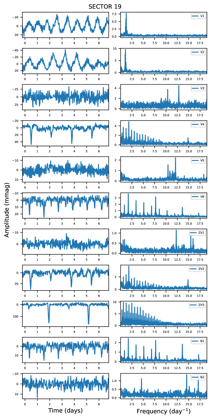
Figure 32: The Sector 19 LCs and the corresponding frequency spectra of known variables in NGC 2126.

The frequency analysis for the variable stars in TESS data was done using the program Period04 (Lenz & Breger, 2004). We adopted the criteria SNR $>=5.6$ given by Zong et al. (2016) for space-based observations. The SNR was calculated after prewhitening all of the dominant frequencies to obtain the residual spectra, followed by calculating the noise using a box size of one cycle per day along both sides of the target frequency. The errors in frequency and amplitude were calculated using the analytical relations provided by Montgomery & O’Donoghue (1999). The Appendix Table. 9 & 10 list the frequencies for the known variables detected using TESS and from the ground and the light curves in the respective sectors are plotted in Fig. 32, 33 and 34.

6.1 Contamination

The large pixel size of TESS causes the blending of signals from nearby sources. The resulting LCs for a target can only be trusted when (i) the source is much brighter than the nearby contaminating sources so that the background source only adds to the noise and (ii) the contaminating sources are non-variables and, hence, only increase the noise level rather than introduce signals in the periodogram.

In order to investigate the contamination in TESS LCs, we first overplotted the Gaia sources on the target pixel file (TPF) in the vicinity of each target to see if there are any bright nearby objects that might potentially contribute to contamination. After that, we selected a variety of custom apertures to determine the origin of a specific set of frequencies within the frequency spectrum. An example of this investigation is shown in Figure 9, where V551 Aur (V6) is a pulsating EB that is contaminated with a $\delta$ Scuti star (N1). Next, we cross-checked whether any of these frequencies are predefined in the ground-based data obtained from Chehlaeh et al. (2018). For, example in case of V6 in Fig. 9, the two strong blue peaks towards the right were detected by Chehlaeh et al. (2018) for N1 and few of the dominant red peaks to the left were reported by Chehlaeh et al. (2018) for V6.

We found that two of the pulsating stars ZV2 (hybrid star) and N1 ($\delta$ Scuti star) were contaminated significantly by the nearby binary stars V4 and V6 respectively and found that the contamination can be addressed with the above technique. Furthermore, to quantify the extent of contamination endured by the variable stars detected in our study, we calculated a contamination factor for each of these stars using Gaia DR3 positions and magnitudes, where we took the ratio of the target flux to the total flux in a 21^′′ radius.

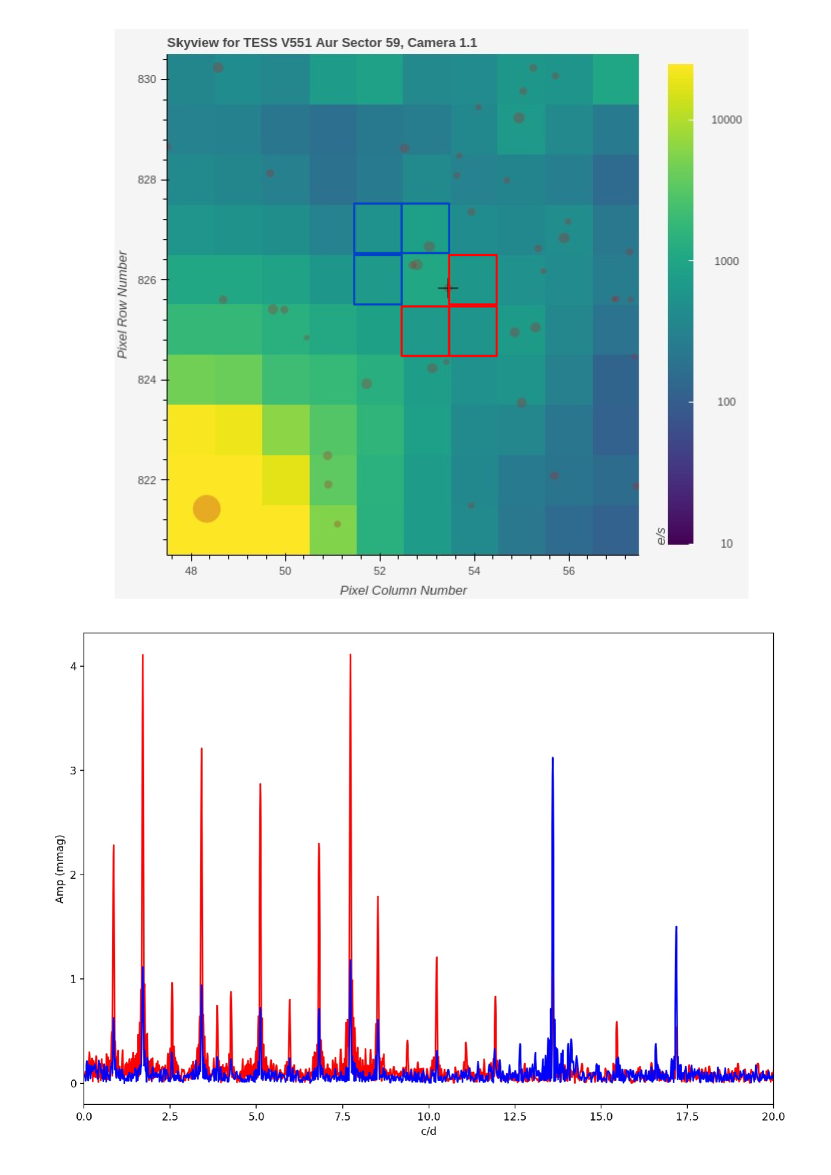
Figure 9: The top panel depicts the TPF of star V6 overlaid with nearby Gaia DR3 targets. V551 Aur (V6) is identified with a black ‘+’ symbol. Custom apertures were chosen near V6 (marked with red boxes) and N1 (marked with blue boxes). The bottom panel depicts the periodogram generated by the two apertures, V6 in red and N1 in blue, which are superimposed on each other. The harmonic signals and pulsation are stronger in the red aperture and weaker in the blue aperture. The two dominant frequency signals in blue behave in opposite ways, indicating they are from the nearby star N1.

7 CLASSIFICATION OF VARIABLE STARS

Variable stars are classified according to the shape of their LCs, amplitude of variability, frequency of variability, and location on the HR diagram. The pulsating stars can be identified from the HR diagram by plotting the instability strips for $\delta$ Scuti and $\gamma$ Doradus pulsator. In our study, we used the theoretical $\delta$ Scuti and $\gamma$ Doradus instability strips, computed by Dupret et al. (2005).

The standard B- and V-band magnitudes from our ground-based observations with the 1.3-m DFOT were used to generate the HR diagram for the cluster members. After extinction correction, the color index B-V was used to find the effective temperature ($T_{\rm eff}$), which was based on an empirical relationship from Torres (2010). Next, the empirical relation provided by Torres (2010) was employed to calculate the bolometric correction ($BC_{v}$) for the stars in the V-band. Then the luminosity can be estimated using the standard relations, where we took bolometric magnitude of sun as $M_{bol_{\odot}}$ = 4.73 (Torres, 2010). The HR diagram in Fig. 10 shows the known variables, the newly found variables, and the instability strips for the $\delta$ Scuti and $\gamma$ Doradus pulsations.

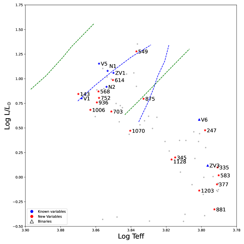
Figure 10: HR-diagram for the member stars based on the ground-based observations. Blue ‘star’ symbols and the blue triangles indicate the known pulsating variables and the EBs respectively. The red ‘star’ symbols represent the newly detected variable stars. The green and blue dashed lines represent the edges of the theoretical $\delta$ Scuti and $\gamma$ Doradus instability strips, respectively, computed by Dupret et al. (2005).

$\gamma$ Doradus variables are mainly non-radial $g$-mode pulsators showing periodic variations in their brightness with pulsation frequencies ranging from 0.5 to 3 d^-1 (Aerts et al., 2010) and amplitude of variation up to 0.1 mag in the V-band. The convective blocking drives the $g$-mode pulsations, with buoyancy as the restoring force (Dupret et al., 2005). In the HR diagram, the $\gamma$ Doradus instability strip is seen overlapped with the cooler edge of the $\delta$ Scuti instability strip in the main sequence with an early F spectral type.

$\delta$ Scuti stars are primarily $p$-mode pulsators with brightness variations ranging from 0.001 to 0.8 mag in the V band and pulsation frequencies ranging from 5 to 50 d^-1 (Aerts et al., 2010). The $\kappa$-mechanism drives the pulsations in these stars, which occur at the partial ionization zones in the outer radiative region (Pamyatnykh, 2000). These stars are found at the lower part of the classical instability strip, which intersects the main sequence, called the $\delta$ Scuti instability strip. They are A- to early F-type stars with masses ranging from 1.5 to 2.5 $M_{\odot}$. They pulsate in both radial and non-radial $p$-modes. Some of the stars pulsate both in $g$-modes and $p$-modes, with characteristics similar to $\gamma$ Doradus and $\delta$ Scuti stars. These stars are known as hybrid pulsators (Handler et al., 2009).

The G- and K-type stars are located below the $\delta$ Scuti and $\gamma$ Doradus instability strips. These stars, with a convective envelope, exhibit rotational variability due to spots on their surface (Mamajek & Hillenbrand, 2008). The LCs of these rotational variables produces a frequency spectrum with the rotational frequency below 5 d^-1 and at least one harmonic of the rotational frequency (Balona, 2013). Thus we classified the main sequence variables with a frequency less than 5 d^-1 falling in the G to K spectral type as rotational variables. Also in this region one can find the solar type oscillations. The stars whose LCs show (partial or full) eclipses can be classified as EBs.

All of the member stars, as well as those with LCs in both TESS and ground-based observations, were classified according to the criteria listed above. Table 4 shows the results for newly discovered member stars, while Table 5 shows the results for stars with variability in TESS and ground-based observations. We observe that ground-based classification is incomplete due to insufficient data.

Table 4: The newly detected variable cluster members are listed with their ID, RA, DEC, standard magnitude, first dominant frequency used for phase folding, corresponding semi-amplitude, assigned variability type, membership, and contamination in TESS.

ID	RA	DEC	Mag	Frequency	Amp	Variability type	Mem.	Cont.
	(deg)	(deg)	(mag)	(d-1)	(mag)		(%)	(%)
72	90.5885	49.752833	17.423	2.796	0.022	-	90.8	49.40
124	90.527917	49.767417	18.18	1.905	0.029	-	85.8	0
143	90.567028	49.775222	13.817	5.690	0.009	DSCT	75.2	0
247	90.657528	49.808472	14.785	4.224	0.010	-	77.3	33.17
335	90.711278	49.831306	15.739	5.234	0.009	-	70.9	3.79
345	90.536139	49.832639	15.455	3.016	0.009	-	61.9	3.44
377	90.607278	49.84275	16.169	4.231	0.011	ROT	57.3	89.78
549	90.663472	49.881278	12.743	1.741	0.024	-	89.8	51.58
568	90.606944	49.884222	13.752	5.119	0.005	DSCT	54.9	89.35
614	90.643167	49.889639	13.465	6.062	0.006	DSCT	64.8	46.79
703	90.680778	49.90125	14.264	4.722	0.005	-	74.4	37.33
752	90.6185	49.908417	13.916	4.948	0.005	-	69.8	20.28
875	90.610778	49.929528	13.949	3.202	0.005	GDOR	76.3	7.07
881	90.857528	49.932306	16.802	2.568	0.008	ROT	83.1	38.97
1006	90.611389	49.966889	14.22	3.906	0.005	-	74.8	1.89
1070	90.679444	49.983611	14.756	4.359	0.005	-	50.5	3.21
1128	90.437278	49.997917	15.505	2.907	0.012	-	82.7	24.59
1203	90.778667	50.015194	16.312	3.284	0.055	ROT	90.2	3.19
DSCT : $\delta$ Scuti, GDOR : $\gamma$ Doradus, ROT : Rotational variable

Table 5: The variables detected in TESS with their ID’s, names (if any), the orbital or rotational period ($P$(d)) from TESS, the pulsational period ($P_{pul}$(d)) from TESS, assigned variability type, membership from Gaia DR3 (Mem.) and TESS contamination (Cont.). The error values at the last digit are represented inside brackets for the periods.

ID	Name	RA	DEC	$P$(d)	$P_{pul}$(d)	Variability	Mem.	Cont.
						Type	(%)	(%)
V1	V546 Aur	90.433639	49.941861	-	0.8094(2)	GDOR	68.7	0.24
V2	V547 Aur	90.488972	49.982056	-	0.9394(2)	GDOR	-	0.37
V3	V548 Aur	90.521556	49.819861	-	0.078040(6)	DSCT	-	6.38
V4	V549 Aur	90.588583	49.877167	3.300284(1)	-	EB	-	88.50
V5	V550 Aur	90.609806	49.865889	-	0.082706(7)	DSCT	-	7.36
V6	V551 Aur	90.658250	49.884250	1.1731767(4)	0.129453(8)	EB + DSCT	76.5	88.52
ZV1	UCAC4 700-043212	90.637472	49.880111	-	0.08161(1)	DSCT	51.6	15.05
ZV2	UCAC4 700-043178	90.590278	49.873361	-	0.067336(9)	Hybrid	-	38.08
ZV3	UCAC4 700-043174	90.584750	49.806611	3.224040(2)	-	EB	83.7	59.84
N1	UCAC4 700-043245	90.661139	49.879417	-	0.073534(4)	DSCT	61.8	65.29
N2	UCAC4 700-043196	90.614056	49.845361	-	0.068719(9)	DSCT	70.7	10.51
839	-	90.648306	49.920833	0.7390(3)	-	ROT	-	2.17
DSCT : $\delta$ Scuti, GDOR : $\gamma$ Doradus, EB : Eclipsing Binary, ROT : Rotational variable

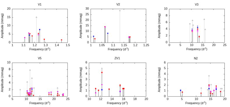
Figure 11: Representation of the results of the frequency analysis of the TESS data of the stars without contamination. The filled circles with error bars in blue, red, and magenta show the observed amplitudes in the TESS data of sectors 19, 59, and 73, respectively. They are compared to those published by Chehlaeh et al. (2018) (grey upward triangles) and Zhang et al. (2012) (grey downward triangles), if available.

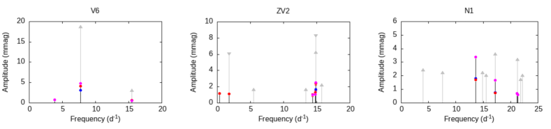
Figure 12: Same as Fig. 11, but for stars affected by contamination.

7.1 Intrinsic Variables

7.1.1 $\gamma$ Doradus Stars

NGC 2126 contains two known $\gamma$ Doradus variables (V1 and V2). Our membership analysis revealed that V2 is not likely to be a cluster member. The two stars were detected by TESS. Both stars have a frequency lower than 3 c/d. Fig. 11 shows a comparison of our results with previous frequency estimates from the literature. There were no harmonics of the fundamental frequency in the frequency spectrum, showing that they are not rotational variables. The position of V1 in the HR diagram is within the $\gamma$ Doradus instability strip. Since, V2 is not a member star, we used the Gaia temperature $T_{\rm eff}$= 7134 K, indicating it is an early F-type star. Thus, we classify V1 and V2 as $\gamma$ Doradus variables. From our ground observations, we classified the star 875, as $\gamma$ Doradus variable, based on the frequency and position in the HR diagram. The TESS data for this star produced null results.

7.1.2 $\delta$ Scuti Stars and Hybrid Pulsators

Chehlaeh et al. (2018) reported six $\delta$ Scuti stars (V3, V5, ZV1, N1, N2) and a hybrid pulsator (ZV2). All of these stars were detected in TESS data. ZV1, N1, and N2 were determined to be probable cluster members. Fig. 11 and Fig. 12 show a comparison between the frequencies detected in literature and those we detected from TESS’s three sectors. Pulsation frequencies in ZV1, N1 and N2 were similar to those of a $\delta$ Scuti star, ranging from 5 to 30 c/d. They belong to the $\delta$ Scuti instability strip on the HR diagram. Thus, we classify these stars as $\delta$ Scuti stars. However, N1 is contaminated by a nearby binary star V6. To address this we used the method described in the previous section. Since, V3 and V5 are not cluster members we used the Gaia temperatures, V3 has $T_{\rm eff}$= 7454 K, while V5 has $T_{\rm eff}$= 6166 K, this corresponds to a spectral type F. The spectral type along with the pulsation frequencies from TESS indicates these are $\delta$ Scuti stars. According to Zhang et al. (2012), ZV2 is a hybrid pulsator because it has a low frequency of 1.812 d^-1in addition to the $\delta$ Scuti type frequencies. Our analysis of TESS data recovered the dominant frequency 14.851 d^-1 , as well as the low frequency reported by Zhang et al. (2012). As ZV2 is not a member, we used the Gaia temperature, $T_{\rm eff}$= 7081 K, indicating an F-type star. This means the star is in the $\gamma$ Doradus instability strips where $\delta$ Scuti instability strip also overlaps. Thus, we classify it as a hybrid pulsator. This star was also contaminated by a nearby EB, V4. We used the method described in previous section in this case also to identify the frequencies. Using ground-based data, we identified three new $\delta$ Scuti variables, 143, 568, and 614. The classification was made based on their positions in the HR diagram and oscillation frequencies. TESS detected no signals from these stars due to high contamination.

7.2 Extrinsic Variables

7.2.1 Rotational Variable

We discovered a new variable, 839, in the field of NGC 2126. The star shows variable signals on the ground, as well as TESS data. Fig. 13 compares the TESS LC and frequency spectra of this star. This star demonstrates TESS’s improved frequency resolution. The dominant frequency is the same in both spectra, however, the ground-based spectrum has many aliases. The frequency is less than 5 c/d and appears as harmonics in the TESS frequency spectra. The Gaia temperature, $T_{\rm eff}$= 5725, indicates a G-type star. Thus, we classify this star as a rotational variable. From the ground-based observations, we also identified three additional rotational variables, 377, 881, and 1203. We were unable to detect any of these stars using TESS due to contamination.

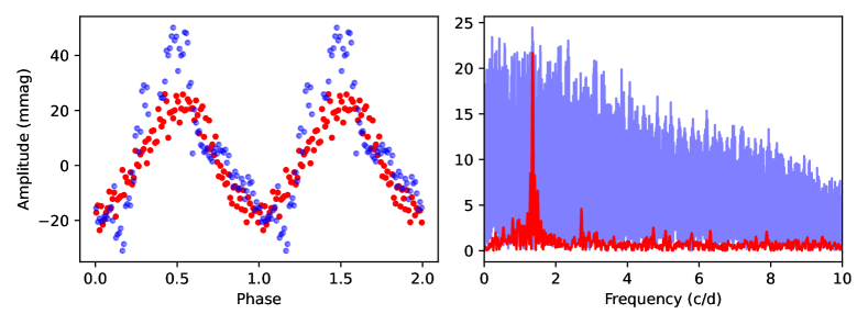
Figure 13: Left panel shows the LCs for the newly detected rotational variable 839 phase folded to the dominant peak in its frequency spectrum and binned with a bin size of 0.02 in phase. The red points are from TESS Sector 19 and the blue points are from the ground-based observations. In the right panel, the corresponding frequency spectra for the respective LCs are given. We see the advantage of frequency resolution from TESS compared to the ground-based.

7.2.2 Eclipsing Binaries

Chehlaeh et al. (2018) identified three EBs in NGC 2126, V4, V6, and ZV3. They were able to cover a large enough phase range for two stars, V4 and V6, allowing them to model the LCs and derive basic parameters such as orbital periods, inclination, mass ratio, and temperature ratio. For ZV3, however, modeling and period determination were not possible due to a lack of data covering the full eclipse. We used continuous time series TESS observations to fully cover the three EBs’ phase range in our study. ZV3 and V6 are members of the cluster, while V4 is not a member. Given the cluster membership, the case of V6 is more interesting because it is a pulsating EB.

According to available data, Chehlaeh et al. (2018) estimated an orbital period of 1 to 1.5 days for ZV3. However, with the help of TESS data that included multiple eclipses, we were able to calculate the orbital period for this star. We used all of the primary minima found in sectors 19, 59, and 73 by fitting a parabola to their dips. To determine the system’s linear ephemeris, the orbital cycle vs. time of minima (TOM) curve was fitted with a linear relation.

The resulting linear ephemeris for ZV3 is :

$$\begin{split}BJD_{min}&=2458818.0594\pm 0.0008\\ &\quad+3.224040\pm 0.000002\times E\end{split}$$ (6)

where $BJD_{min}$ is the time of primary minima at epoch E. Fig. 14 shows the epheremis fit.

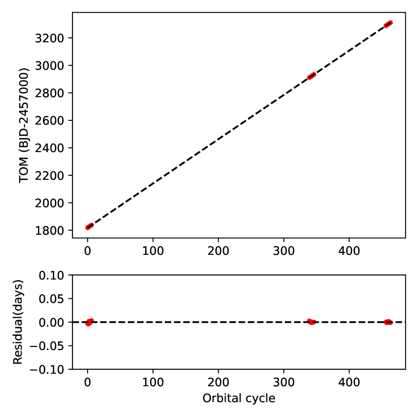
Figure 14: The top panel shows the orbital cycle vs. times of primary minima (TOM) detected from all the three TESS Sectors. The dashed line is the straight line fit to this data. The bottom panel shows the residuals of the fit.

For V4, Chehlaeh et al. (2018) discovered an orbital period of 3.300281 days. We collected LCs for this star from TESS sectors 19, 59, and 73. In addition to the primary minima detected from TESS sectors, two minima reported in Chehlaeh et al. (2018) were included in the ephemeris fit.

The subsequent linear ephemeris for V4 is :

$$\begin{split}BJD_{min}&=2452308.388\pm 0.002\\ &\quad+3.300284\pm 0.000001\times E\end{split}$$ (7)

Gáspár et al. (2003) described V6 as an EB with a pulsating component. Chehlaeh et al. (2018) revisited the nature of this variable star, as well as the parameters of the open cluster that hosts it. They concluded that the pulsation could be caused by tidally excited $g$-modes, which exhibit tidal resonance with the orbital period. Although previous research concluded that V551 Aur is unlikely to belong to the open cluster, our analysis of Gaia DR3 data revealed that it most likely does. As in the previous case, we determined the linear ephemeris from all the primary minima detected in TESS sectors, as well as the ground-based minima listed in Table 9 of Chehlaeh et al. (2018).

The final linear ephemeris for V6 is:

$$\begin{split}BJD_{min}&=2452307.410\pm 0.003\\ &\quad+1.1731767\pm 0.0000004\times E\end{split}$$ (8)

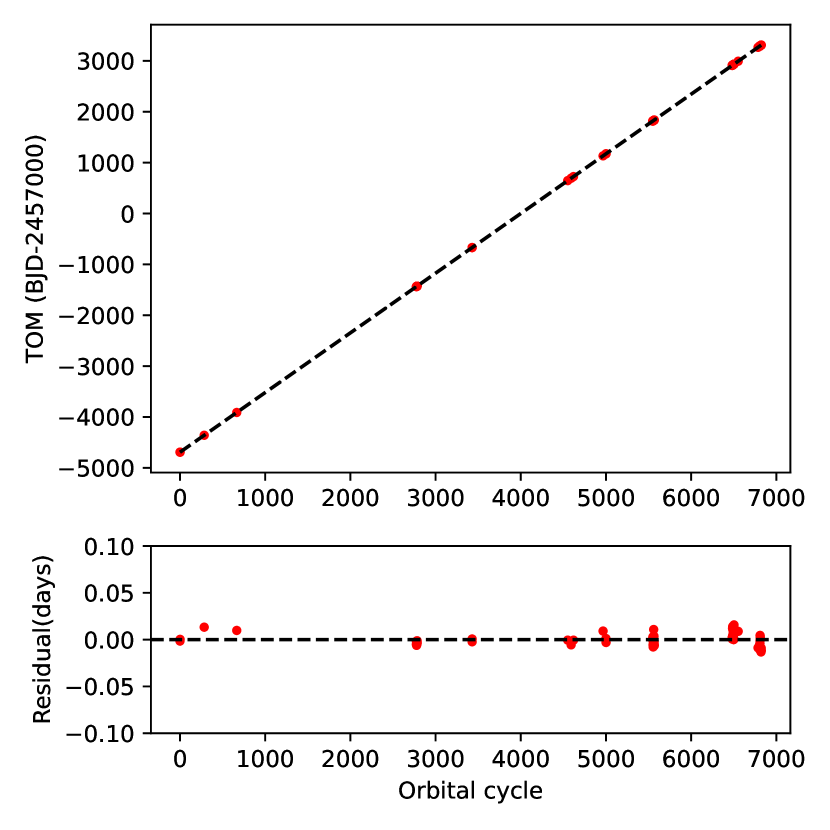
Figure 35: The top panel shows the linear ephemeris of V551 Aur by fitting a straight line to the observed times of primary minima (TOM) from all the TESS sectors along with the ground-based minima detected in this study and listed in Chehlaeh et al. (2018). The bottom panel shows the residuals of the fit.

Fig. 15 depicts the phased and binned TESS LCs for three EBs. Appendix Fig. 35 & 36 shows the ephemeris fit for V6 and V4, respectively.

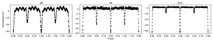
Figure 15: From left to right each panel shows the phased LCs of V6, V4 and ZV3, using all the available TESS sectors (19, 59 and 73) and binned using a bin size 0.002 in phase. For V6 we can clearly see the pulsations on top of the eclipses.

8 Eclipsing Binary Modeling

EBs provide an independent method for calculating stellar masses and radii. By modeling the eclipsing LCs and the radial velocity curve, we can determine the best fitting parameters for masses, radii, inclination, and so on. However, we only have TESS LCs for our EBs. Due to the faintness of these stars, no high-resolution spectra could be obtained using the facilities we have direct access to. Thus we used the eclipsing LCs alone to model our EBs. While modelling the EB LC, one should take care of the intrinsic variability that it may possess either due to some intrinsic process in the system such as pulsations, mass transfer, star spots etc. (Pigulski, 2006) or external reasons like telescope systematics or contamination in case of TESS. Therefore, it was imperative to incorporate the intrinsic variability or long-term systematics into the LC modeling process.

The primary and secondary minima of all three of our EBs (V4, V6, and ZV3) are clearly distinct, with the out-of-eclipse region flat and the secondary minima precisely located at the 0.5 phase of the orbital period. Consequently, it is reasonable to assume that they are detached binaries in a circular orbit. We modeled the intrinsic variability in EB LCs using the celerite package (Foreman-Mackey et al., 2017; Foreman-Mackey, 2018). This package is part of the exoplanet package (Foreman-Mackey et al., 2021) and features a scalable Gaussian process model with a SHOTerm (a term representing a stochastically-driven, damped harmonic oscillator). This package has the capability to simultaneously model the intrinsic variability with a scalable Gaussian process and the eclipses for a detached binary system. The exoplanet code employs PyMC (Fonnesbeck et al., 2015) for its probabilistic modeling. It utilizes the starry package (Luger et al., 2019) to generate limb-darkened LCs and employs a fast and efficient solver for Kepler’s equations.

The q-search method (Wilson, 1994; Joshi et al., 2016a) can be employed to estimate the mass ratio (q-value) of the system in the absence of spectroscopic data. Previous studies by Liu et al. (2012) and Chehlaeh et al. (2018) calculated the mass ratio for V6 and V4, respectively, using the photometric q-search method using the PHOEBE 1.0 legacy version based on Wilson-Devinney code (Prša & Zwitter, 2005). We used the q-values calculated for V4 and V6 from previous studies. For ZV3, we used a similar approach and calculated the q-value with PHOEBE 1.0. The best fitting q-value was $q$ = 0.48 based on the q-value vs. chi square plot, as shown in Fig. 16.

These photometrically derived q-values served as priors for modeling the EB LCs. The primary star’s mass was determined by comparing evolutionary tracks on the HR diagram, and the radius was calculated using the Stefan-Boltzmann’s relation, with the primary star’s temperature being the B-V color temperature in the case of V4 and ZV3. For V6, we used the spectroscopic temperature obtained through medium-resolution spectroscopy.

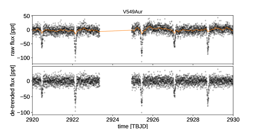
Figure 37: Top panel shows the Gaussian process model of V549 Aur. Bottom panel shows the residuals after subtracting the model

The Appendix Table. 11 contains the prior distributions that were chosen for modeling in the exoplanet code. Table. 6 provide the best fit parameters for binary modeling for all stars, which were compared to previous estimates by Chehlaeh et al. (2018). Fig. 17, 18, 19 depict the best-fit LCs. Fig. 37, 38, 39, and Fig. 20, 40, 41 show the Gaussian process fits and corner plots, respectively.

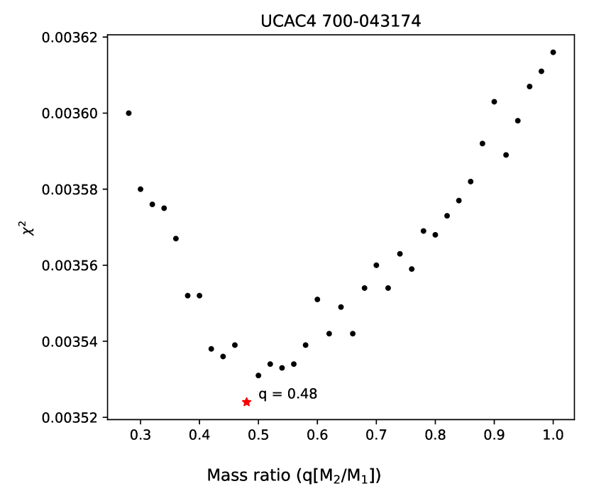
Figure 16: The figure shows the $q$ (mass ratio) search for UCAC4 700-043174 (ZV3) using PHOEBE 1.0 legacy version. The $q$ value with minimum $\chi^{2}$ is marked with a red asterisk and was chosen for further modeling.

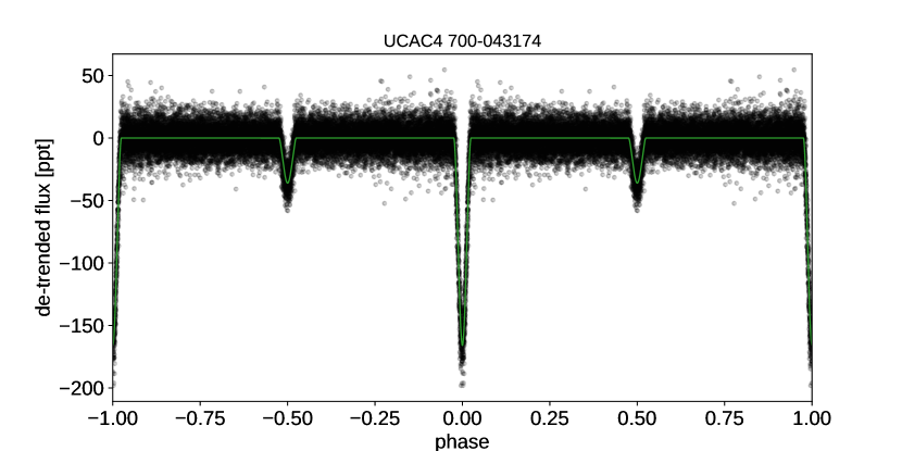
Figure 17: The phased folded LC of UCAC4 700-043174 (ZV3) with the best fitting model.

Table 6: The parameters computed with exoplanet code for ZV3, V4 and V6 are given in the table. $T_{0}$ is the time of primary minima, $q$ is the mass ratio, $i$ is the inclination, $k$ is the radius ratio, $e$ is eccentricity and $s$ is the surface brightness ratio. The last two terms are the Gaussian process parameters, $\rho_{gp}$ represents the undamped period of the oscillator and $\sigma_{gp}$ the standard deviation of the process.

Star	Parameter	This work	Chehlaeh et al.
			(2018)
	Period (days)	3.224040 (fixed)	-
	$T_{0}$ (BJD)	2458818.0594 (fixed)	-
	$q$	0.480(5)	-
	$i$ (deg)	82.10(9)	-
ZV3	k	1.0(2)	-
	$e$	0.04(4)	-
	$s$	0.20(9)	-
	$\rho_{gp}$	1.0(2)	-
	$\sigma_{gp}$	1.7(2)	-
	Period (days)	3.300284 (fixed)	3.300281(1)
	$T_{0}$ (BJD)	2452308.388 (fixed)	-
	$q$	0.626(6)	0.626(7)
	$i$ (deg)	80.4(2)	86.61(6)
V4	$k$	0.6(2)	-
	$e$	0.13(5)	0 (fixed)
	$s$	2(1)	-
	$\rho_{gp}$	0.23(2)	-
	$\sigma_{gp}$	4.9(2)	-
	Period (days)	1.1731767 (fixed)	1.1731752(8)
	$T_{0}$ (BJD)	2452307.410 (fixed)	-
	$q$	0.769(8)	0.769(5)
	$i$ (deg)	61.8(7)	73.01(6)
V6	$k$	0.90(9)	-
	$e$	0.02(1)	0 (fixed)
	$s$	0.8(2)	-
	$\rho_{gp}$	0.116(5)	-
	$\sigma_{gp}$	5.3(2)	-

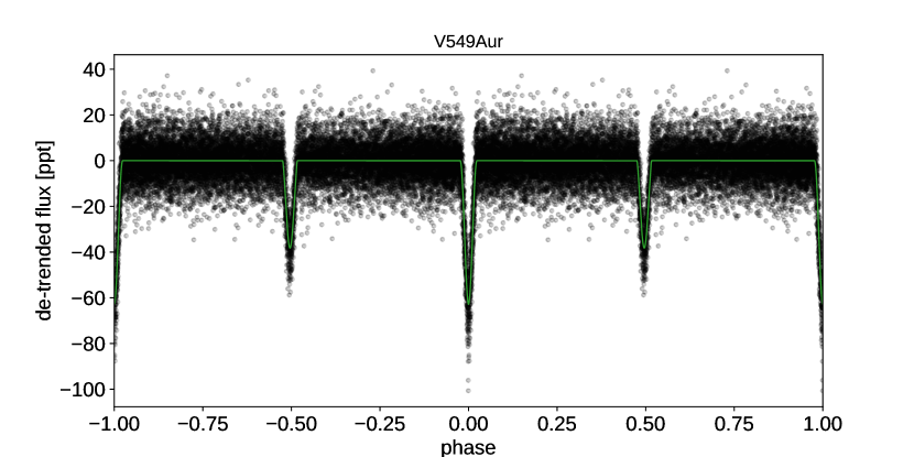
Figure 18: The phased folded LC of V549 Aur (V4) with the best fitting model.

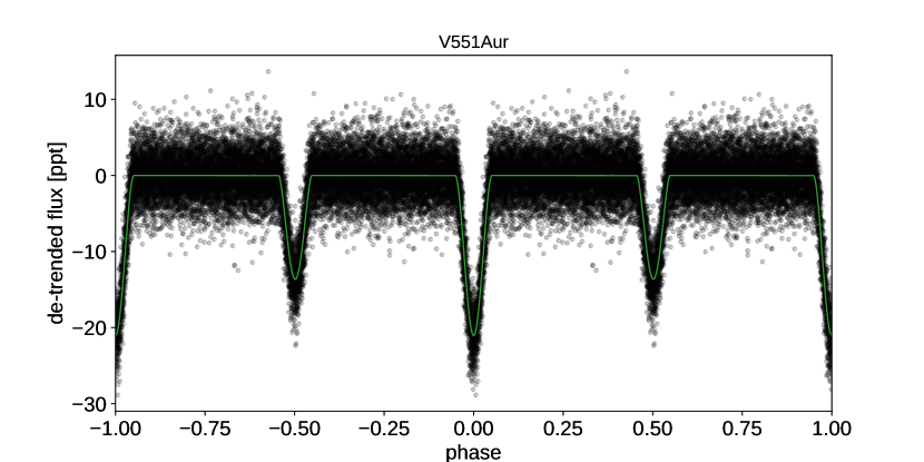
Figure 19: The phased folded LC of V551 Aur (V6) with the best fitting model.

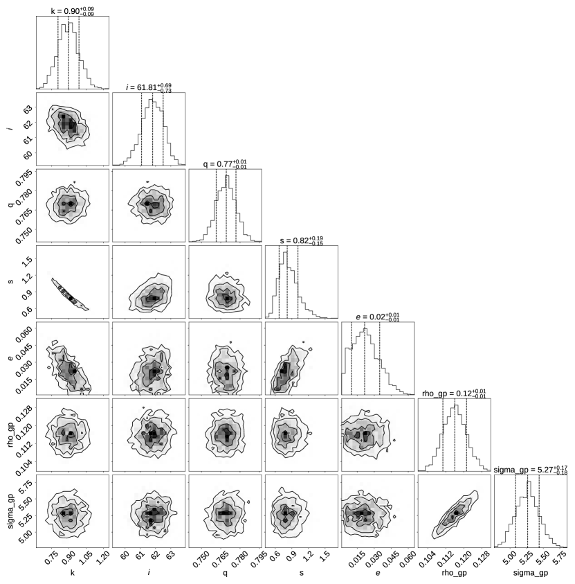
Figure 20: The resultant posterior distribution for the eclipse model and the Gaussian process model for the best fit from exoplanet code for V551 Aur.

8.1 V551 Aur : A pulsating eclipsing binary

V551 Aur is an EB that exhibits pulsational variability in its LC. Previous authors proposed that the variability could be due to pulsations in the binary system’s primary component. However, the nature and origin of this star’s pulsation remain poorly understood. The associated frequency, 7.7248(5), is very close to the $9^{th}$ harmonic of the orbital frequency, so the pulsation may be a higher order resonance with the orbital frequency. This could indicate a tidally excited $g$-mode on the primary star. The companions’ nature is unknown because no spectroscopic observations have been made.

As described in the previous section, we modelled both eclipses and intrinsic variability simultaneously. The pulsational frequency, first harmonics, second harmonics, and sub-harmonics were identified in the residuals of the eclipse model subtracted LC (refer to Fig. 21). The presence of a subharmonic frequency in the pulsation indicates that the pulsations are non-linear, which is not expected from a pure stable oscillator. This lends credence to the theory that the pulsation in one of the companions is caused by tidal forces. The ground-based phased LC (Fig. 22) shows that during the secondary eclipse, pulsations dominate, indicating that the pulsating member is the primary companion.

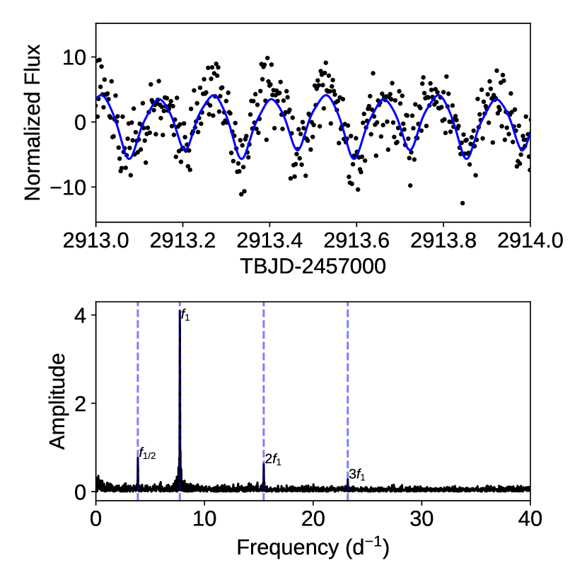
Figure 21: The top panel is the residuals after removing the binary model from the LC of V551 Aur. Here only the pulsation signals is seen. The bottom panel shows the frequency spectrum of the residual. Apart from the dominant peak being the pulsation frequency, one can notice the first two harmonics and a sub-harmonics in the spectrum.

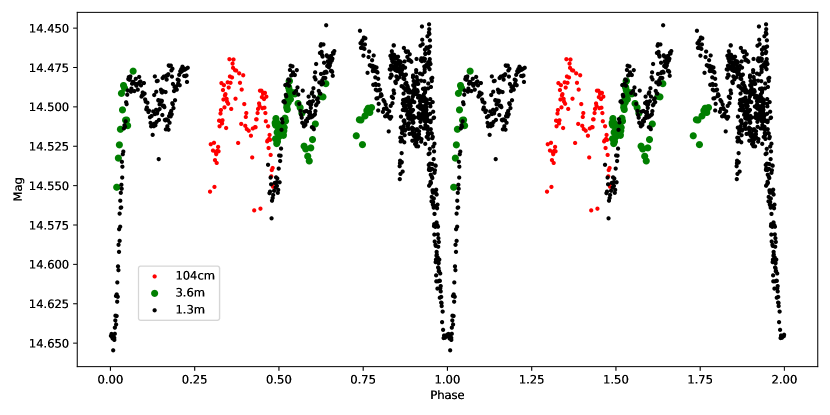
Figure 22: Ground-based phase folded LC of V551 Aur using the orbital period determined from TESS. The red, green and black data points represents the data taken with 104 cm Sampurnanand, 3.6 m DOT and 1.3 m DFOT telescopes respectively at ARIES, Nainital.

8.2 Spectroscopy

Low-resolution spectroscopic observations for V551 Aur were carried out with Himalayan Chandra telescope, Hanle Faint Object Spectrograph Camera (HFOSC) (Cowsik et al., 2002), during 2021 and 2022. A total of 16 spectra with a resolution of R $\sim$ 1200 were obtained during different phases of the orbital period. The radial velocities proved to be unreliable for our study because of the low-resolution and due to the fact that the components’ profiles are always blended and furthermore affected by the pulsation. However, close examination of the strong Balmer lines shows significant line profile variations across different phases (see Fig. 23 for the H$\alpha$ lines) indicating a spectroscopic binary. A series of high-resolution spectra is required to construct the star’s radial velocity curves, which will provide accurate system parameters. Because we do not have direct access to the spectroscopic observational facilities required to observe a $14^{th}$ magnitude star, we propose this as a future project. We used the low-resolution spectra to determine the basic parameters of the star by comparison with synthetic spectra (Table. 12), using the chi-square minimization technique employed in GSSP code (Tkachenko, 2015).

A medium-resolution spectrum was taken with the 2.4-m Telescope, Thailand National Observatory (TNO), Thailand, Medium-Resolution Spectrograph with a resolution of R$\sim$18,000 over a range of 380-900 nm. The H$\beta$ line (Fig. 24) was used to calculate the $T_{\rm eff}$  and $\log g$  by comparison with synthetic spectra using the GSSP code. Due to binarity and poor resolution, the metallicity estimation is unreliable and cannot be compared to the cluster metallicity. To improve the signal-to-noise ratio of the line profile, we applied the Least Square Deconvolution (LSD) method (Donati et al., 1997). The LSD profile (Fig. 25) was used to calculate the $v\sin i$ and radial velocity of the star. The best fit results of our analysis are presented in Table. 7.

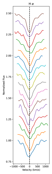
Figure 23: The H$\alpha$ line of low-resolution spectra at different phases obtained with HFOSC equipped on HCT. The normalized flux for each spectra was added by 0.1 for visual clarity. The phase increases from 0 to 1 from bottom to top.

Table 7: The table shows the spectroscopic parameters that were found for V551 Aur using the medium-resolution spectrum. The parameters were found by fitting synthetic spectra to the H$\beta$ line and line profile fitting to the LSD profile.

Parameters	Hbeta	LSD
$T_{\rm eff}$	6458 $\pm$ 361 K	-
$\log g$	3.0 $\pm$ 1.49	-
RV	-	-8.4 $\pm$ 1.2 km/s
$v\sin i$	-	44.0 $\pm$ 2.5 km/s

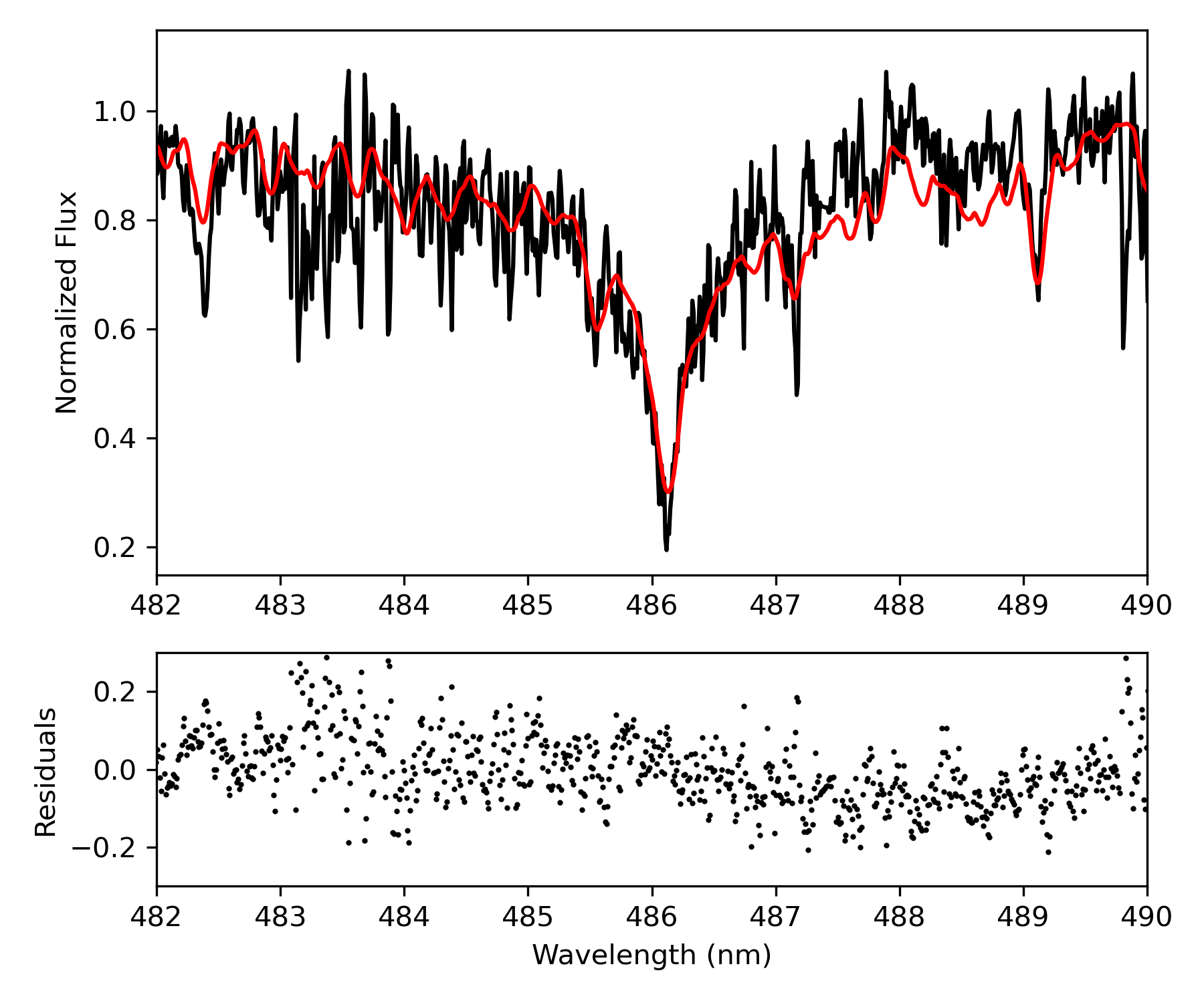
Figure 24: The top panel shows the H$\beta$ line (black) of the medium-resolution spectrum acquired for V551 Aur at an orbital phase 0.96 and the best fit synthetic spectrum (red). The bottom panel shows the residuals of the fit.

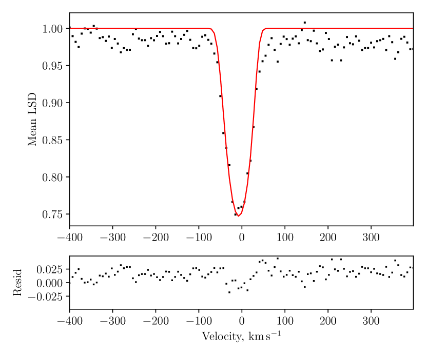
Figure 25: Top panel shows the mean LSD profile of the medium-resolution spectra (black) for V551 Aur. A rotationally broadened line profile (red) was fit to this data to find vsini and radial velocity. The bottom panel gives the residuals of the fit.

9 SUMMARY

Our ground-based observations revealed 25 member variables and 85 field variables within a 9 arcmin radius field of NGC 2126. Our research was focused on member variables and stars with promising LCs in the TESS data. We discovered 18 new variable cluster members from the ground.

In TESS, we identified counterparts for 11 known variables, including six members and five field stars. Furthermore, we identified a new field star as a rotational variable based on TESS LC. TESS frequency spectra show distinctive pulsation peaks, especially for $\delta$ Scuti stars. These frequencies can be used to conduct asteroseismic studies on member pulsating stars. Aside from that, the cluster has a higher metallicity than the solar metallicity, implying the presence of chemically peculiar stars in the cluster. Thus, a spectroscopic investigation can benefit our understanding of the member variables.

We attempted to solve the TESS contamination problem by using custom apertures for our sources and cross-matching detected frequencies to ground-based frequencies. This method was useful for stars that produced strong signals in TESS.

We used TESS data to model the EBs V4, V6, and ZV3 by combining their TESS LCs. However, this model still lacks the support of spectroscopic radial velocity measurements. Due to a lack of data, ZV3 had not previously been modeled or its orbital period determined. We utilized the continuous LCs from TESS data to model this star, thereby establishing the linear ephemeris and determining the orbital period.

The intrinsic variability and eclipses of the pulsating EB V551 Aur were modeled simultaneously to determine its parameters. This resulted in slightly different parameter estimates than those reported in previous literature. The low-resolution spectroscopy confirms the spectral line profile variation for this system, indicating that it is a spectroscopic binary. The medium-resolution spectra provided better estimates of spectroscopic parameters for V551 Aur.

10 CONCLUSIONS

This project was initiated to search and study pulsating variables in the open star cluster NGC 2126, utilizing ground-based observations, Gaia data and TESS FFIs for improved analysis. This study led us to draw the following conclusions :

• Our study demonstrates that TESS LCs alone are unreliable in the case of open clusters due to contamination. To address this issue and fully utilize the TESS data, one must integrate Gaia data and ground-based observations. This allows us to identify contaminated sources and make better use of the frequency resolution provided by TESS.

• V551 Aur, which was known to exhibit pulsations in one of its components, was found to be a spectroscopic binary with membership to the cluster. To understand this system and model it accurately, high-resolution spectroscopic follow-up observations covering this star’s orbital phase is required. Due to the star’s faintness, we intend to use observations with a larger aperture telescope.

From isochrone fitting, we determined log age $\sim$9.2, a metallicity $\sim$ 0.016, and a distance of $\sim$1.2 kpc for the cluster. Our results are in agreement with previous determinations from Chehlaeh et al. (2018), but with slight differences (log age $\sim$ 9.1, Z $\sim$ 0.019, d $\sim$ 1.4 kpc in Chehlaeh et al. (2018)), possibly due to the improved magnitude, color, proper motion and parallax from Gaia.

Our observations of NGC 2126 are limited to a few nights. More observations are demanding for a detailed frequency analysis of the detected targets. Therefore, we plan to conduct further observations for the cluster using the observing facilities at ARIES, Nainital.

Data Availability

The data underlying in this article will be shared upon request to the corresponding author. This paper includes data collected by the TESS and SIMBAD databases operated by the NASA Explorer Program and CDS, Strasbourg, France, respectively. This work has made use of data from the European Space Agency (ESA) mission Gaia(https://www.cosmos.esa.int/gaia), processed by the Gaia Data Processing and Analysis Consortium (DPAC, https://www.cosmos.esa.int/web/gaia/dpac/consortium). Funding for the DPAC has been provided by national institutions, in particular the institutions participating in the Gaia Multilateral Agreement. This paper includes data collected by the TESS mission, which are publicly available from the Mikulski Archive for Space Telescopes (MAST).

Appendix A Field Stars

Figure 26: The phased V-band LCs of newly detected field variables in NGC 2126. Their respective IDs and periods are given as the title of each figure.

Figure 27: New variables - continued.

Figure 28: New variables - continued.

Figure 29: New variables - continued.

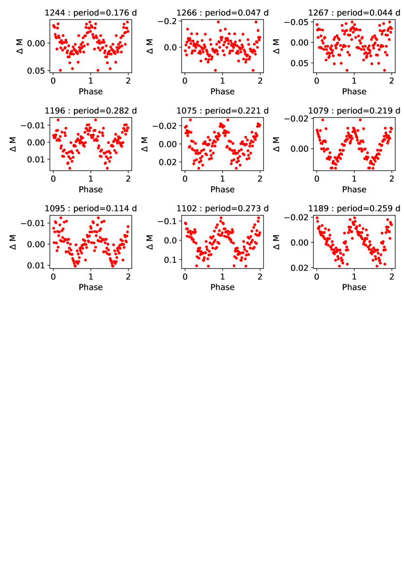
Figure 30: New variables - continued.

Table 8: The newly detected field variables from ground observations are listed with their ID, corrected magnitude, dominant frequency detected and their corresponding amplitudes.

ID	RA	DEC	Mag	Frequency	Amp	ID	RA	DEC	Mag	Frequency	Amp
			(mag)	(d-1)	(mag)				(mag)	(d-1)	(mag)
5	90.693528	49.732833	17.272	2.340	0.027	536	90.857778	49.880417	16.201	2.197	0.010
42	90.818583	49.742389	18.303	0.513	0.073	555	90.452556	49.881361	15.840	2.734	0.011
43	90.720028	49.742278	17.485	0.511	0.063	557	90.442917	49.881528	17.627	2.634	0.020
69	90.807361	49.751944	18.122	1.992	0.062	564	90.689056	49.884472	13.588	1.729	0.011
96	90.649444	49.760167	18.465	2.042	0.036	578	90.490917	49.884139	16.378	3.197	0.010
101	90.792972	49.763167	18.083	0.874	0.075	583	90.712944	49.886389	15.941	0.219	0.013
113	90.806667	49.766194	18.301	2.265	0.033	649	90.758222	49.895194	17.827	3.391	0.030
122	90.430194	49.766194	14.958	1.898	0.022	667	90.747583	49.896778	15.418	1.374	0.013
132	90.841667	49.771611	16.458	2.487	0.018	673	90.831528	49.897778	16.188	4.981	0.012
161	90.663667	49.781611	17.450	2.258	0.038	685	90.529556	49.897194	15.457	2.677	0.008
174	90.683972	49.786639	16.978	1.615	0.034	763	90.857111	49.911806	18.298	2.228	0.120
181	90.815611	49.789611	16.520	1.972	0.024	780	90.870333	49.913639	18.924	2.508	0.048
188	90.691639	49.793500	14.827	2.112	0.018	785	90.445639	49.911389	17.480	10.318	0.020
191	90.770583	49.794667	16.312	1.615	0.031	790	90.626972	49.913194	19.299	3.500	0.073
194	90.868000	49.795333	15.880	2.487	0.018	796	90.487861	49.912889	15.630	1.690	0.006
236	90.814278	49.806944	16.793	1.978	0.016	817	90.450556	49.915833	16.551	5.111	0.008
239	90.580361	49.805833	15.727	2.112	0.011	832	90.689083	49.920194	16.610	7.970	0.015
258	90.855111	49.812944	18.185	1.985	0.050	835	90.456444	49.918833	16.667	4.260	0.012
264	90.769750	49.813583	15.541	1.996	0.011	854	90.704528	49.925222	17.714	2.424	0.052
267	90.624278	49.813194	16.557	1.875	0.030	856	90.469889	49.923417	15.634	3.722	0.010
273	90.665056	49.814778	18.306	1.832	0.030	866	90.495306	49.926917	14.498	0.533	0.019
280	90.606861	49.816028	14.400	2.496	0.007	910	90.795611	49.939806	16.296	2.225	0.029
283	90.738278	49.816972	15.930	1.830	0.017	925	90.532194	49.941667	17.325	3.780	0.020
293	90.554944	49.819472	16.688	2.533	0.017	936	90.445556	49.944222	14.031	0.215	0.005
300	90.638722	49.821000	14.776	1.685	0.009	951	90.835222	49.951389	14.348	2.251	0.012
302	90.700750	49.822222	16.736	2.287	0.020	836	90.466111	49.919111	17.283	4.217	0.015
331	90.569389	49.829278	16.639	2.390	0.016	1039	90.521861	49.974750	15.712	2.263	0.018
394	90.775917	49.849889	17.145	1.973	0.017	1019	90.484417	49.969278	19.470	1.932	0.126
411	90.622750	49.853278	15.926	2.502	0.013	1050	90.847750	49.978333	13.020	2.104	0.014
419	90.515722	49.854000	16.923	2.112	0.025	1055	90.858417	49.980889	16.489	2.538	0.019
420	90.546167	49.854917	14.862	2.281	0.007	1072	90.555861	49.983944	15.467	3.764	0.007
421	90.842778	49.857056	15.732	1.973	0.011	1244	90.781139	50.027389	17.733	2.843	0.033
431	90.828194	49.858472	15.247	2.840	0.018	1266	90.614139	50.031250	19.602	10.637	0.054
456	90.637583	49.862139	16.486	3.967	0.011	1267	90.747306	50.032417	18.748	11.270	0.035
459	90.705750	49.863694	18.543	2.588	0.040	1196	90.541778	50.012444	14.887	1.775	0.017
470	90.518778	49.864222	14.798	2.500	0.007	1075	90.873500	49.987528	17.240	2.263	0.019
489	90.530833	49.868667	16.649	5.008	0.008	1079	90.830778	49.988194	13.016	2.287	0.015
503	90.469333	49.871417	15.547	2.608	0.016	1095	90.619694	49.991056	16.197	4.403	0.010
521	90.653472	49.876083	15.578	5.306	0.005	1102	90.526806	49.991806	18.745	1.829	0.083
529	90.475611	49.875667	16.745	2.573	0.015	1189	90.456472	50.010611	16.340	1.931	0.015

Appendix B Color color diagram

Appendix C TESS Photometry

Table 9: List of detected pulsational frequencies for Sectors 19, 59, and 73 for the stars without contamination. Their respective frequencies, amplitudes and SNR are listed. The significance criterion was based on the minimum Signal-to-Noise ratio of 5.6 and above.

ID	Sector	FrequncyID	Frequency		Amplitude	SNR
			(d-1)		(mmag)
V1	19	$f_{V1,19,1}$	$1.2475\pm 0.0008$		$7.8\pm 0.3$	11.1
		$f_{V1,19,2}$	$1.156\pm 0.001$		$4.5\pm 0.3$	6.4
	59	$f_{V1,59,1}$	$1.2355\pm 0.0003$		$5.53\pm 0.08$	19.2
		$f_{V1,59,2}$	$1.1597\pm 0.0003$		$5.37\pm 0.08$	17.9
		$f_{V1,59,3}$	$1.1804\pm 0.0004$		$4.01\pm 0.08$	13.6
		$f_{V1,59,4}$	$1.2893\pm 0.0008$		$2.00\pm 0.08$	7.0
		$f_{V1,59,5}$	$1.4460\pm 0.0009$		$1.68\pm 0.08$	6.1
	73	$f_{V1,73,1}$	$1.1485\pm 0.0004$		$5.7\pm 0.1$	9.8
		$f_{V1,73,2}$	$1.2362\pm 0.0005$		$4.7\pm 0.1$	8.9
		$f_{V1,73,3}$	$1.1136\pm 0.0008$		$3.0\pm 0.1$	5.1
V2	19	$f_{V2,19,1}$	$1.0771\pm 0.0007$		$8.3\pm 0.3$	13.9
		$f_{V2,19,2}$	$1.013\pm 0.001$		$5.7\pm 0.3$	9.9
		$f_{V2,19,3}$	$1.176\pm 0.001$		$5.1\pm 0.3$	9.3
	59	$f_{V2,59,1}$	$1.0645\pm 0.0002$		$14.3\pm 0.2$	25.9
		$f_{V2,59,2}$	$1.1768\pm 0.0007$		$5.2\pm 0.2$	8.9
		$f_{V2,59,3}$	$1.019\pm 0.001$		$3.6\pm 0.2$	6.1
	73	$f_{V2,73,1}$	$1.0652\pm 0.0003$		$14.0\pm 0.2$	18.9
		$f_{V2,73,2}$	$1.1724\pm 0.0008$		$5.1\pm 0.2$	7.3
V3	19	$f_{V3,19,1}$	$12.816\pm 0.003$		$4.5\pm 0.5$	8.1
		$f_{V3,19,2}$	$10.372\pm 0.003$		$3.7\pm 0.5$	5.5
	59	$f_{V3,59,1}$	$12.814\pm 0.001$		$4.0\pm 0.2$	16.2
		$f_{V3,59,2}$	$10.374\pm 0.001$		$3.4\pm 0.2$	8.3
		$f_{V3,59,3}$	$13.514\pm 0.002$		$1.8\pm 0.2$	6.7
	73	$f_{V3,73,1}$	$10.374\pm 0.002$		$3.6\pm 0.3$	7.8
		$f_{V3,73,2}$	$12.815\pm 0.002$		$3.5\pm 0.3$	7.9
V5	19	$f_{V5,19,1}$	$12.091\pm 0.001$	*	$2.2\pm 0.1$	10.4
		$f_{V5,19,2}$	$10.440\pm 0.002$		$1.6\pm 0.1$	7.5
	59	$f_{V5,59,1}$	$11.4365\pm 0.0003$	*	$2.24\pm 0.03$	34.2
		$f_{V5,59,2}$	$12.0923\pm 0.0004$	*	$1.63\pm 0.03$	27.3
		$f_{V5,59,3}$	$10.4384\pm 0.0006$		$1.06\pm 0.03$	23.5
		$f_{V5,59,4}$	$21.4049\pm 0.0007$		$0.84\pm 0.03$	15.1
		$f_{V5,59,5}$	$11.8053\pm 0.0008$		$0.76\pm 0.03$	12.2
		$f_{V5,59,6}$	$10.8224\pm 0.0009$		$0.70\pm 0.03$	12.9
		$f_{V5,59,7}$	$18.2956\pm 0.0009$		$0.67\pm 0.03$	12.5
		$f_{V5,59,8}$	$19.0526\pm 0.0009$		$0.64\pm 0.03$	13.3
		$f_{V5,59,9}$	$11.3121\pm 0.0009$		$0.64\pm 0.03$	9.7
		$f_{V5,59,10}$	$10.957\pm 0.001$		$0.42\pm 0.03$	7.2
		$f_{V5,59,11}$	$23.452\pm 0.001$		$0.41\pm 0.03$	9.6
		$f_{V5,59,12}$	$21.906\pm 0.002$		$0.38\pm 0.03$	6.5
		$f_{V5,59,13}$	$12.639\pm 0.002$		$0.34\pm 0.03$	6.5
		$f_{V5,59,14}$	$21.325\pm 0.002$		$0.33\pm 0.03$	6.0
	73	$f_{V5,73,1}$	$12.0915\pm 0.0005$	*	$2.54\pm 0.06$	24.0
		$f_{V5,73,2}$	$11.4449\pm 0.0006$	*	$1.79\pm 0.06$	18.9
		$f_{V5,73,3}$	$10.4380\pm 0.0007$		$1.66\pm 0.06$	19.1
		$f_{V5,73,4}$	$21.4070\pm 0.0008$		$1.47\pm 0.06$	12.4
		$f_{V5,73,5}$	$11.8051\pm 0.0009$		$1.29\pm 0.06$	12.3
		$f_{V5,73,6}$	$19.0531\pm 0.0009$		$1.30\pm 0.06$	18.3
		$f_{V5,73,7}$	$18.298\pm 0.001$		$1.16\pm 0.06$	13.5
		$f_{V5,73,8}$	$11.314\pm 0.001$		$1.17\pm 0.06$	12.9
		$f_{V5,73,9}$	$10.824\pm 0.001$		$1.13\pm 0.06$	12.7
		$f_{V5,73,10}$	$10.953\pm 0.001$		$0.92\pm 0.06$	10.3
		$f_{V5,73,11}$	$23.453\pm 0.001$		$0.80\pm 0.06$	9.4
		$f_{V5,73,12}$	$11.372\pm 0.002$		$0.65\pm 0.06$	7.1
		$f_{V5,73,13}$	$23.250\pm 0.002$		$0.50\pm 0.06$	6.1
*Frequency values consistent with Chehlaeh et al. (2018).

Table 9: Continued.

ID	Sector	FrequncyID	Frequency		Amplitude	SNR
			(d-1)		(mmag)
ZV1	19	$f_{ZV1,19,1}$	$12.253\pm 0.002$	*	$1.2\pm 0.1$	9.2
		$f_{ZV1,19,2}$	$15.461\pm 0.003$	*	$0.9\pm 0.1$	6.8
	59	$f_{ZV1,59,1}$	$12.2504\pm 0.0006$	*	$4.3\pm 0.1$	21.9
		$f_{ZV1,59,2}$	$15.458\pm 0.001$	*	$2.0\pm 0.1$	12.6
		$f_{ZV1,59,3}$	$16.120\pm 0.002$		$1.4\pm 0.1$	9.4
		$f_{ZV1,59,4}$	$11.165\pm 0.002$		$1.4\pm 0.1$	7.9
		$f_{ZV1,59,5}$	$15.943\pm 0.002$		$1.4\pm 0.1$	9.5
		$f_{ZV1,59,6}$	$13.512\pm 0.002$		$1.3\pm 0.1$	6.1
		$f_{ZV1,59,7}$	$11.660\pm 0.003$		$1.1\pm 0.1$	5.8
	73	$f_{ZV1,73,1}$	$12.2531\pm 0.0008$	*	$2.11\pm 0.08$	16.0
		$f_{ZV1,73,2}$	$15.461\pm 0.002$	*	$0.97\pm 0.08$	6.8
		$f_{ZV1,73,3}$	$11.171\pm 0.003$		$0.65\pm 0.08$	5.2
N2	19	$f_{N2,19,1}$	$14.552\pm 0.002$		$1.4\pm 0.1$	7.3
		$f_{N2,19,2}$	$17.094\pm 0.003$		$1.3\pm 0.1$	7.8
		$f_{N2,19,3}$	$4.608\pm 0.003$		$1.1\pm 0.1$	6.1
	59	$f_{N2,59,1}$	$14.5554\pm 0.0007$	*	$2.09\pm 0.07$	22.7
		$f_{N2,59,2}$	$17.0921\pm 0.0008$		$1.89\pm 0.07$	21.1
		$f_{N2,59,3}$	$16.304\pm 0.001$		$1.10\pm 0.07$	13.6
		$f_{N2,59,4}$	$18.627\pm 0.002$		$0.89\pm 0.07$	10.0
		$f_{N2,59,5}$	$15.134\pm 0.002$		$0.82\pm 0.07$	9.5
		$f_{N2,59,6}$	$5.206\pm 0.002$		$0.79\pm 0.07$	5.7
		$f_{N2,59,7}$	$11.785\pm 0.003*$		$0.61\pm 0.07$	6.1
		$f_{N2,59,8}$	$15.098\pm 0.003$		$0.57\pm 0.07$	6.6
		$f_{N2,59,9}$	$15.774\pm 0.003$		$0.49\pm 0.07$	5.9
	73	$f_{N2,73,1}$	$14.554\pm 0.001$	*	$1.89\pm 0.09$	14.5
		$f_{N2,73,2}$	$17.088\pm 0.001$	*	$1.55\pm 0.09$	17.0
		$f_{N2,73,3}$	$16.301\pm 0.002$		$1.08\pm 0.09$	9.9
		$f_{N2,73,4}$	$15.138\pm 0.002$		$0.91\pm 0.09$	6.8
839	19	$f_{839,19,1}$	$1.3530\pm 0.0006$		$21.6\pm 0.6$	15.0
		$f_{839,19,2}$	$2.715\pm 0.003$		$4.5\pm 0.6$	5.2
*Frequency values consistent with Chehlaeh et al. (2018).

Table 10: List of detected pulsational frequencies for Sectors 19, 59 and 73 for the stars that are contaminated. Their respective frequencies, amplitudes and SNR are listed. The significance criterion was based on the minimum Signal-to-Noise ratio of 5.6 and above.

ID	Sector	FrequncyID	Frequency		Amplitude	SNR
			(d-1)		(mmag)
V6	19	$f_{V6,19,1}$	$7.7248\pm 0.0005$	*	$3.08\pm 0.07$	46.8
	59	$f_{V6,59,1}$	$7.7266\pm 0.0004$	*	$4.10\pm 0.07$	41.5
		$f_{V6,59,1}/2$	$3.862\pm 0.002$		$0.75\pm 0.07$	8.2
		$2f_{V6,59,1}$	$15.450\pm 0.002$	*	$0.63\pm 0.07$	7.9
	73	$f_{V6,73,1}$	$7.7270\pm 0.0002$	*	$4.77\pm 0.06$	49.3
		$f_{V6,73,1}/2$	$3.864\pm 0.002$		$0.74\pm 0.06$	7.8
		$2f_{V6,73,1}$	$15.454\pm 0.002$	*	$0.56\pm 0.06$	8.8
ZV2	19	$f_{ZV2,19,1}$	$14.851\pm 0.002$	*	$1.6\pm 0.2$	7.7
	59	$f_{ZV2,59,1}$	$14.852\pm 0.001$	*	$2.4\pm 0.2$	14.2
		$f_{ZV2,59,2}$	$14.802\pm 0.003$		$1.3\pm 0.2$	7.9
		$f_{ZV2,59,3}$	$14.409\pm 0.003$		$1.0\pm 0.2$	6.8
		$f_{ZV2,59,4}$	$0.318\pm 0.002$		$1.2\pm 0.1$	5.8
		$f_{ZV2,59,5}$	$1.815\pm 0.002$	**	$1.1\pm 0.1$	5.7
	73	$f_{ZV2,73,1}$	$14.8394\pm 0.0008$	*	$2.53\pm 0.09$	26.1
		$f_{ZV2,73,2}$	$14.405\pm 0.002$		$1.01\pm 0.09$	10.3
		$f_{ZV2,73,3}$	$14.793\pm 0.002$		$1.07\pm 0.09$	11.0
N1	19	$f_{N1,19,1}$	$13.5991\pm 0.0008$	*	$1.81\pm 0.07$	19.4
		$f_{N1,19,2}$	$17.176\pm 0.003$	*	$0.76\pm 0.07$	10.4
	59	$f_{N1,59,1}$	$13.5969\pm 0.0009$	*	$1.70\pm 0.07$	19.7
		$f_{N1,59,2}$	$17.177\pm 0.002$	*	$0.74\pm 0.07$	8.4
	73	$f_{N1,73,1}$	$13.5972\pm 0.0003$	*	$3.38\pm 0.05$	28.4
		$f_{N1,73,2}$	$17.1767\pm 0.0006$	*	$1.67\pm 0.05$	24.6
		$f_{N1,73,3}$	$21.203\pm 0.001$	*	$0.71\pm 0.05$	9.1
		$f_{N1,73,4}$	$21.348\pm 0.002$		$0.59\pm 0.05$	7.8
*Frequency values consistent with Chehlaeh et al. (2018).
**Frequency values consistent with Zhang et al. (2012).

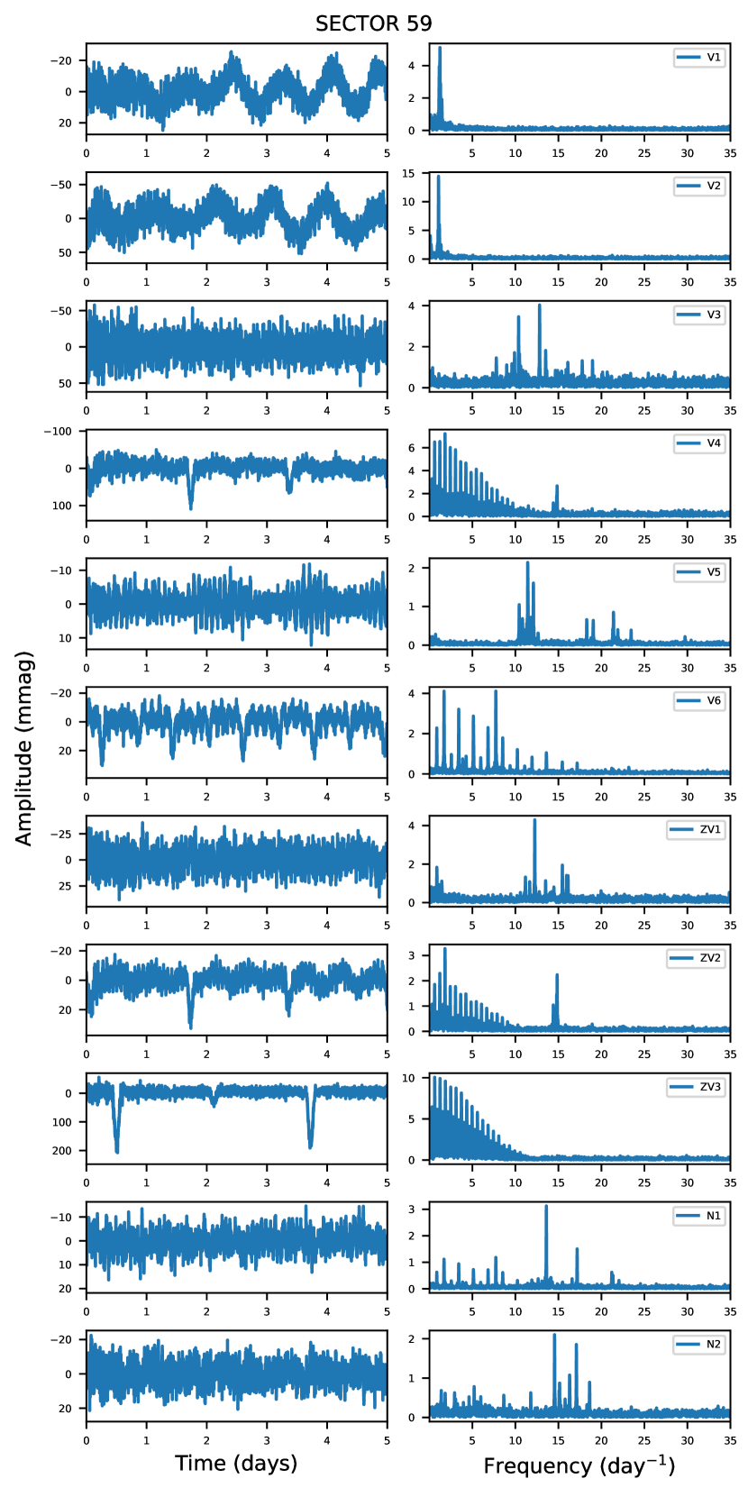
Figure 33: The Sector 59 LCs and the corresponding frequency spectra of known variables in NGC 2126.

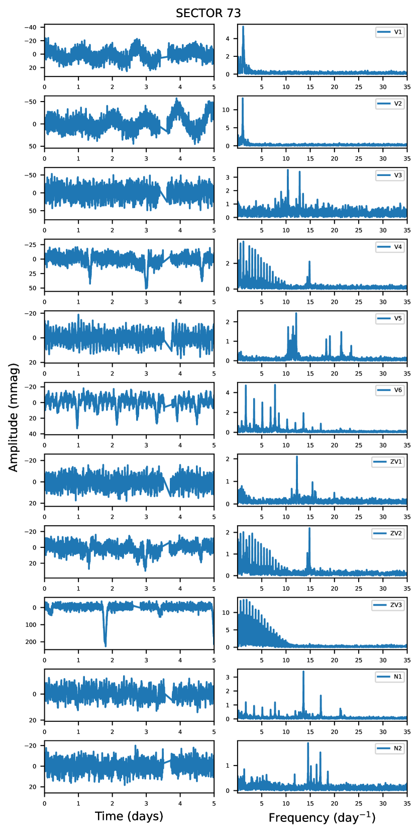
Figure 34: The Sector 73 LCs and the corresponding frequency spectra of known variables in NGC 2126.

Appendix D Binary Ephermeris

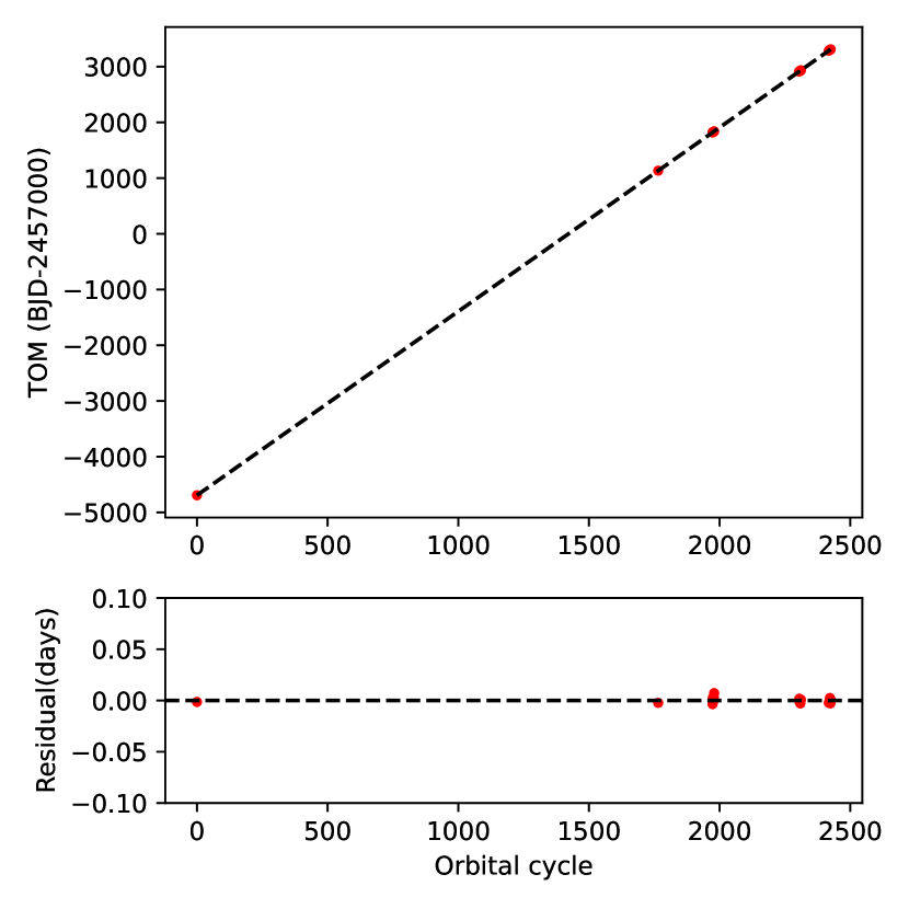
Figure 36: The top panel shows the linear ephemeris of V549 Aur by fitting a straight line to the observed time of primary minima (TOM) from all the TESS sectors and two eclipse minima given in Chehlaeh et al. (2018). The bottom panel shows the residuals of the fit.

Appendix E EB modeling

Table 11: The table gives the adopted prior distributions for the PyMC3 runs with 6000 samples. Here, $M1$ is the mass of the primary star, $R1$ is the radius of the primary star, $k$ is the radius ratio, $q$ is the mass ratio, $s$ is the surface brightness ratio and $ecs$ represents the two orthogonal components of eccentricity $e\cos{\omega}$ and $e\sin{\omega}$.

Parameters	V6	V4	ZV3
$log\_M1$	Normal(log(1.375), 1.0)	Normal(log(1.05), 1.0)	Normal(log(1.20), 1.0)
$log\_R1$	Normal(log(1.728), 1.0)	Normal(log(0.83), 1.0)	Normal(log(1.039), 1.0)
$log\_k$	Normal(0.0, 10.0)	Normal(0.0, 10.0)	Normal(0.0, 10.0)
$log\_q$	Normal(log(0.769), 0.01)	Normal(log(0.626), 0.01)	Normal(log(0.48), 0.01)
$log\_s$	Normal(log(0.5), 10.0)	Normal(log(0.5), 10.0)	Normal(log(0.5), 10.0)
$ecs$	UnitDisk([1e-5, 0.0])	UnitDisk([1e-5, 0.0])	UnitDisk([1e-5, 0.0])

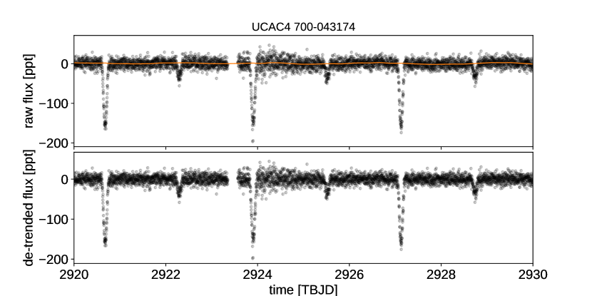
Figure 38: Top panel shows the Gaussian process model of V549 Aur. Bottom panel shows the residuals after subtracting the model

Figure 39: The top panel shows the Gaussian process model of V551 Aur for the pulsational variability. The bottom panel shows the residual LC after subtracting the pulsation model.

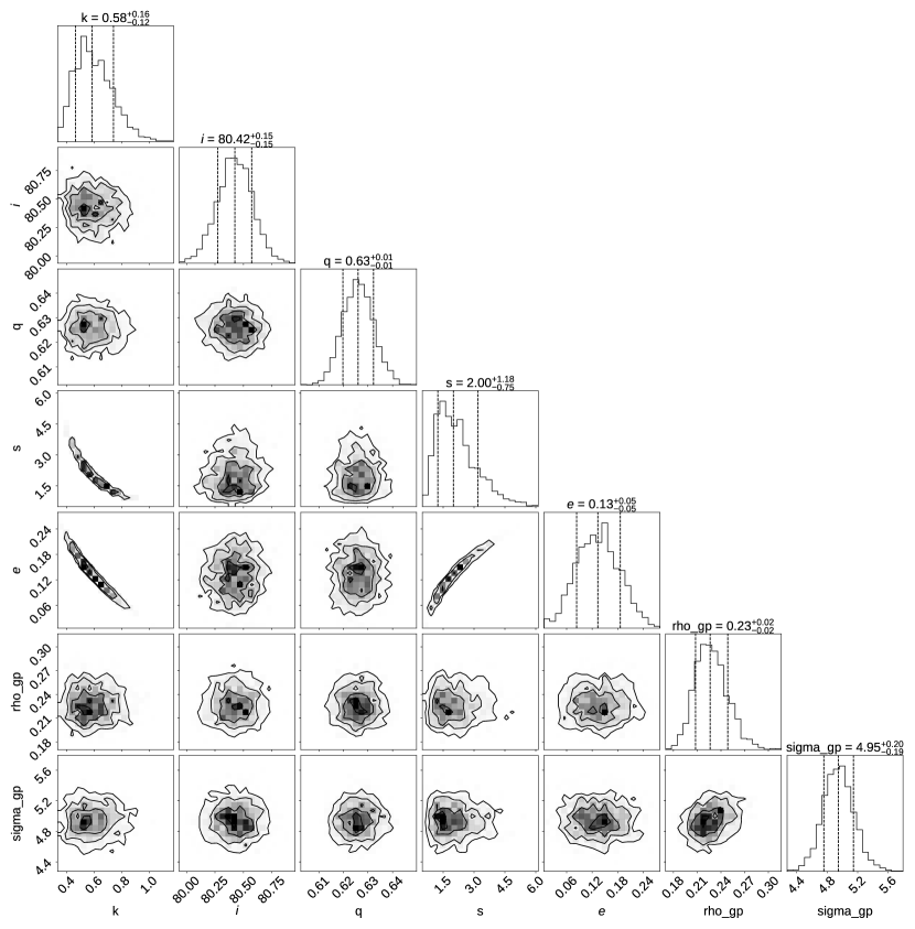
Figure 40: Figure shows the posterior distribution for the eclipse model and Gaussian process model from exoplanet code for V549 Aur.

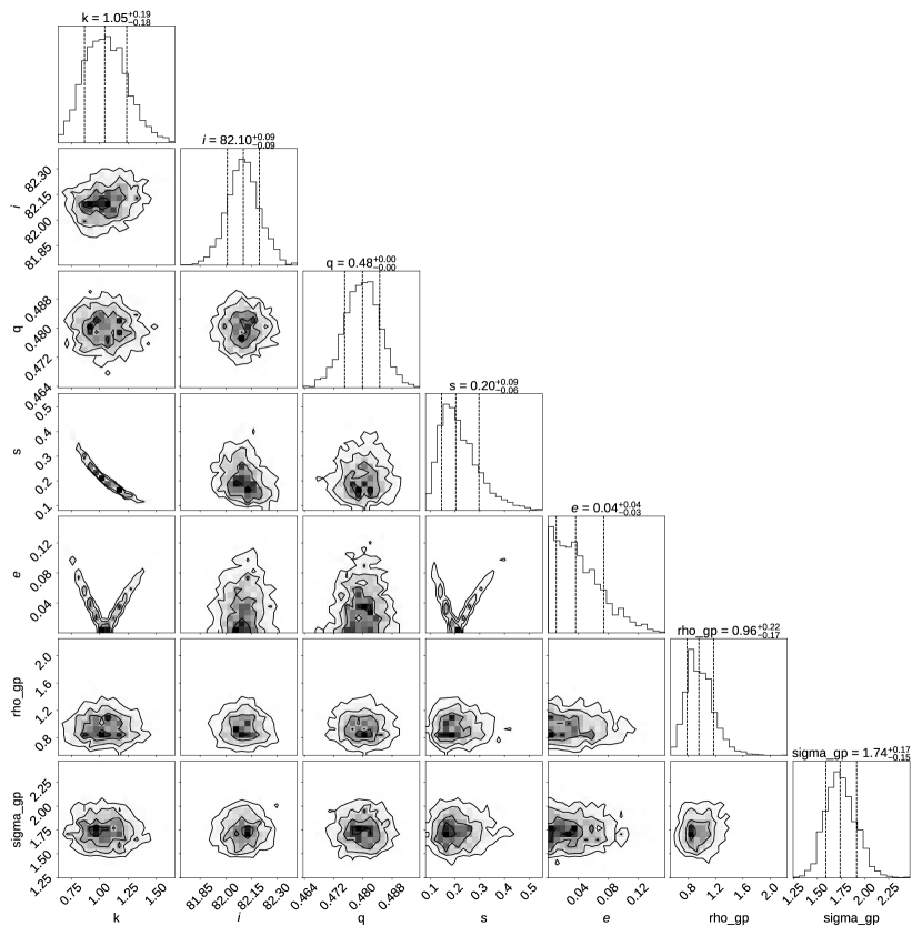
Figure 41: Figure shows the posterior distribution for the eclipse model and the Gaussian process model from exoplanet code for ZV3.

Appendix F Low resolution spectroscopy

Table 12: The table lists the effective temperature ($T_{\rm eff}$) and surface gravity ($\log g$) using Gaia DR3 gsphot and the series of low-resolution spectra. The values of $T_{\rm eff}$ and $\log g$ were derived by fitting the observed spectra with synthetic spectra. The last row gives the mean $T_{\rm eff}$ and $\log g$ values of those derived from the individual spectra.

Source	$T_{\rm eff}$	$\log g$
Gaia DR3 (gsphot)	5943	4.0
Low-resolution
spectrum (this study)
2021-08-15	5853 $\pm$ 213	3 $\pm$ 1
2021-09-13	5898 $\pm$ 178	4 $\pm$ 1
2021-09-18	5938 $\pm$ 177	3 $\pm$ 1
2021-09-19	5792 $\pm$ 213	3 $\pm$ 1
2021-10-05	5868 $\pm$ 299	4 $\pm$ 3
2021-10-12	5792 $\pm$ 272	4 $\pm$ 2
2021-10-19	5772 $\pm$ 424	3 $\pm$ 3
2021-10-22	5832 $\pm$ 348	4 $\pm$ 3
2021-10-26	5746 $\pm$ 221	3 $\pm$ 1
2021-11-15	5898 $\pm$ 173	3 $\pm$ 1
2021-11-21	5878 $\pm$ 365	3 $\pm$ 3
2021-12-08	5853 $\pm$ 247	4 $\pm$ 2
2021-12-20	5777 $\pm$ 211	3 $\pm$ 1
2022-01-03	5640 $\pm$ 241	3 $\pm$ 2
2022-02-08	5827 $\pm$ 252	3 $\pm$ 1
2022-02-17	5853 $\pm$ 208	3 $\pm$ 1
mean	5826 $\pm$ 262	3$\pm$ 2

References

- Aerts (2021) Aerts C., 2021, Reviews of Modern Physics, 93, 015001
- Aerts et al. (2010) Aerts C., Christensen-Dalsgaard J., Kurtz D. W., 2010, Asteroseismology. Berlin: Springer, doi:10.1007/978-1-4020-5803-5
- Ashoka et al. (2000) Ashoka B. N., et al., 2000, Bulletin of the Astronomical Society of India, 28, 251
- Balona (2013) Balona L. A., 2013, MNRAS, 431, 2240
- Bedding et al. (2023) Bedding T. R., et al., 2023, ApJ, 946, L10
- Brasseur et al. (2019) Brasseur C. E., Phillip C., Fleming S. W., Mullally S. E., White R. L., 2019, Astrocut: Tools for creating cutouts of TESS images, Astrophysics Source Code Library, record ascl:1905.007
- Bressan et al. (2012) Bressan A., Marigo P., Girardi L., Salasnich B., Dal Cero C., Rubele S., Nanni A., 2012, MNRAS, 427, 127
- Charbonneau (1995) Charbonneau P., 1995, ApJS, 101, 309
- Chehlaeh et al. (2018) Chehlaeh N., Mkrtichian D., Lampens P., Komonjinda S., Kim S. L., Van Cauteren P., Kusakin A. V., Glazunova L., 2018, MNRAS, 480, 1850
- Chen et al. (2014) Chen Y., Girardi L., Bressan A., Marigo P., Barbieri M., Kong X., 2014, MNRAS, 444, 2525
- Chen et al. (2015) Chen Y., Bressan A., Girardi L., Marigo P., Kong X., Lanza A., 2015, MNRAS, 452, 1068
- Cowsik et al. (2002) Cowsik R., Srinivasan R., Prabhu T., 2002, in Vernin J., Benkhaldoun Z., Muñoz-Tuñón C., eds, Astronomical Society of the Pacific Conference Series Vol. 266, Astronomical Site Evaluation in the Visible and Radio Range. p. 424
- Danielski et al. (2018) Danielski C., Babusiaux C., Ruiz-Dern L., Sartoretti P., Arenou F., 2018, A&A, 614, A19
- Deb & Singh (2009) Deb S., Singh H. P., 2009, A&A, 507, 1729
- Dileep et al. (2024) Dileep A., Joshi S., Kurtz D. W., 2024, Bulletin de la Societe Royale des Sciences de Liege, 93, 227
- Donati et al. (1997) Donati J. F., Semel M., Carter B. D., Rees D. E., Collier Cameron A., 1997, MNRAS, 291, 658
- Dupret et al. (2005) Dupret M. A., Grigahcène A., Garrido R., Gabriel M., Scuflaire R., 2005, A&A, 435, 927
- Feinstein et al. (2019) Feinstein A. D., et al., 2019, PASP, 131, 094502
- Fonnesbeck et al. (2015) Fonnesbeck C., Patil A., Huard D., Salvatier J., 2015, PyMC: Bayesian Stochastic Modelling in Python, Astrophysics Source Code Library, record ascl:1506.005
- Foreman-Mackey (2018) Foreman-Mackey D., 2018, Research Notes of the American Astronomical Society, 2, 31
- Foreman-Mackey et al. (2017) Foreman-Mackey D., Agol E., Ambikasaran S., Angus R., 2017, AJ, 154, 220
- Foreman-Mackey et al. (2021) Foreman-Mackey D., et al., 2021, arXiv e-prints, p. arXiv:2105.01994
- Gaia Collaboration et al. (2016) Gaia Collaboration et al., 2016, A&A, 595, A1
- Gaia Collaboration et al. (2023) Gaia Collaboration et al., 2023, A&A, 674, A1
- Gáspár et al. (2003) Gáspár A., et al., 2003, A&A, 410, 879
- Han & Brandt (2023) Han T., Brandt T. D., 2023, The Astronomical Journal, 165, 71
- Handler et al. (2009) Handler G., et al., 2009, ApJ, 698, L56
- Joshi et al. (2003) Joshi S., et al., 2003, Monthly Notices of the Royal Astronomical Society, 344, 431
- Joshi et al. (2006) Joshi S., Mary D. L., Martinez P., Kurtz D. W., Girish V., Seetha S., Sagar R., Ashoka B. N., 2006, Astronomy and Astrophysics, 455, 303
- Joshi et al. (2009) Joshi S., Mary D. L., Chakradhari N. K., Tiwari S. K., Billaud C., 2009, Astronomy and Astrophysics, 507, 1763
- Joshi et al. (2010) Joshi S., Ryabchikova T., Kochukhov O., Sachkov M., Tiwari S. K., Chakradhari N. K., Piskunov N., 2010, Monthly Notices of the Royal Astronomical Society, 401, 1299
- Joshi et al. (2012) Joshi S., et al., 2012, Monthly Notices of the Royal Astronomical Society, 424, 2002
- Joshi et al. (2016a) Joshi Y. C., Jagirdar R., Joshi S., 2016a, Research in Astronomy and Astrophysics, 16, 63
- Joshi et al. (2016b) Joshi S., et al., 2016b, Astronomy and Astrophysics, 590, A116
- Joshi et al. (2017) Joshi S., Semenko E., Moiseeva A., Sharma K., Joshi Y. C., Sachkov M., Singh H. P., Yerra B. K., 2017, Monthly Notices of the Royal Astronomical Society, 467, 633
- Joshi et al. (2020a) Joshi Y. C., Maurya J., John A. A., Panchal A., Joshi S., Kumar B., 2020a, MNRAS, 492, 3602
- Joshi et al. (2020b) Joshi Y. C., John A. A., Maurya J., Panchal A., Kumar B., Joshi S., 2020b, MNRAS, 499, 618
- Joshi et al. (2022a) Joshi Y. C., Bangia T., Jaiswar M. K., Pant J., Reddy K., Yadav S., 2022a, Journal of Astronomical Instrumentation, 11, 2240004
- Joshi et al. (2022b) Joshi S., et al., 2022b, Monthly Notices of the Royal Astronomical Society, 510, 5854
- King (1962) King I., 1962, The Astronomical Journal, 67, 471
- Kumar et al. (2018) Kumar B., et al., 2018, Bulletin de la Societe Royale des Sciences de Liege, 87, 29
- Lampens (2021) Lampens P., 2021, Galaxies, 9, 28
- Landolt (1992) Landolt A. U., 1992, AJ, 104, 340
- Lata et al. (2023) Lata S., et al., 2023, MNRAS, 520, 1092
- Lenz & Breger (2004) Lenz P., Breger M., 2004, in Zverko J., Ziznovsky J., Adelman S. J., Weiss W. W., eds, IAU Symposium Vol. 224, The A-Star Puzzle. pp 786–790, doi:10.1017/S1743921305009750
- Li et al. (2024) Li G., et al., 2024, A&A, 686, A142
- Lightkurve Collaboration et al. (2018) Lightkurve Collaboration et al., 2018, Lightkurve: Kepler and TESS time series analysis in Python, Astrophysics Source Code Library (ascl:1812.013)
- Liu et al. (2012) Liu N., Zhang X.-B., Ren A.-B., Deng L.-C., Luo Z.-Q., 2012, Research in Astronomy and Astrophysics, 12, 671
- Luger et al. (2019) Luger R., Agol E., Foreman-Mackey D., Fleming D. P., Lustig-Yaeger J., Deitrick R., 2019, AJ, 157, 64
- Mamajek & Hillenbrand (2008) Mamajek E. E., Hillenbrand L. A., 2008, ApJ, 687, 1264
- Martinez et al. (2001) Martinez P., et al., 2001, Astronomy and Astrophysics, 371, 1048
- Maurya et al. (2023) Maurya J., Joshi Y. C., Panchal A., Gour A. S., 2023, AJ, 165, 90
- Montgomery & O’Donoghue (1999) Montgomery M. H., O’Donoghue D., 1999, Delta Scuti Star Newsletter, 13, 28
- Murphy (2019) Murphy S. J., 2019, Pulsating stars in binary systems: a review, doi:10.5281/zenodo.2533474, https://doi.org/10.5281/zenodo.2533474
- Pamos Ortega et al. (2023) Pamos Ortega D., Mirouh G. M., García Hernández A., Suárez Yanes J. C., Barceló Forteza S., 2023, A&A, 675, A167
- Pamyatnykh (2000) Pamyatnykh A. A., 2000, in Breger M., Montgomery M., eds, Astronomical Society of the Pacific Conference Series Vol. 210, Delta Scuti and Related Stars. p. 215 (arXiv:astro-ph/0005276), doi:10.48550/arXiv.astro-ph/0005276
- Panchal et al. (2023) Panchal A., Joshi Y. C., De Cat P., Lampens P., Goswami A., Tiwari S. N., 2023, MNRAS, 521, 677
- Pandey et al. (2018) Pandey S. B., Yadav R. K. S., Nanjappa N., Yadav S., Reddy B. K., Sahu S., Srinivasan R., 2018, Bulletin de la Societe Royale des Sciences de Liege, 87, 42
- Perren et al. (2015) Perren G. I., Vázquez R. A., Piatti A. E., 2015, A&A, 576, A6
- Pigulski (2006) Pigulski A., 2006, in Aerts C., Sterken C., eds, Astronomical Society of the Pacific Conference Series Vol. 349, Astrophysics of Variable Stars. p. 137
- Poznanski et al. (2012) Poznanski D., Prochaska J. X., Bloom J. S., 2012, MNRAS, 426, 1465
- Prša & Zwitter (2005) Prša A., Zwitter T., 2005, ApJ, 628, 426
- Ricker (2014) Ricker G. R., 2014, The Journal of the American Association of Variable Star Observers, 42, 234
- Sarkar et al. (2024) Sarkar M., et al., 2024, Monthly Notices of the Royal Astronomical Society, p. stae2258
- Stetson (1987) Stetson P. B., 1987, PASP, 99, 191
- Stetson (1992) Stetson P. B., 1992, in Worrall D. M., Biemesderfer C., Barnes J., eds, Astronomical Society of the Pacific Conference Series Vol. 25, Astronomical Data Analysis Software and Systems I. p. 297
- Tang et al. (2014) Tang J., Bressan A., Rosenfield P., Slemer A., Marigo P., Girardi L., Bianchi L., 2014, MNRAS, 445, 4287
- Tkachenko (2015) Tkachenko A., 2015, A&A, 581, A129
- Torres (2010) Torres G., 2010, AJ, 140, 1158
- Trust et al. (2021) Trust O., Jurua E., De Cat P., Joshi S., Lampens P., 2021, MNRAS, 504, 5528
- Trust et al. (2023) Trust O., Mashonkina L., Jurua E., De Cat P., Tsymbal V., Joshi S., 2023, MNRAS, 524, 1044
- Wilson (1994) Wilson R. E., 1994, PASP, 106, 921
- Wu et al. (2002) Wu Z. Y., Tian K. P., Balaguer-Núñez L., Jordi C., Zhao L., Guibert J., 2002, A&A, 381, 464
- Yadav et al. (2022) Yadav R. K. S., et al., 2022, Journal of Astronomical Instrumentation, 11, 2240006
- Zhang et al. (2012) Zhang X. B., Deng L. C., Luo C. Q., 2012, AJ, 144, 141
- Zong et al. (2016) Zong W., Charpinet S., Vauclair G., Giammichele N., Van Grootel V., 2016, A&A, 585, A22