Hilbert metric and quasiconformal mappings
Abstract.
We prove a functional identity between the Hilbert metric and the visual angle metric in the unit disk. The proof utilizes the Poincaré hyperbolic metric in terms of which both metrics can be expressed. This identity then yields sharp distortion results for quasiregular mappings and analytic functions, expressed in terms of the Hilbert metric. We also prove that Hilbert circles are, in fact, Euclidean ellipses. The proof makes use of computer algebra methods. In particular, Gröbner bases are used.
Key words and phrases:
Quasiconformal mappings, Möbius transformations, hyperbolic geometry, Hilbert metric, Visual angle metric2010 Mathematics Subject Classification:
30C621. Introduction
In recent years, hyperbolic metrics and metrics similar to it have become standard tools of geometric function theory [DHV, FRV, GH, HIMPS, H, HKV]. In his work [P, pp.42-48], the author comprehensively lists twelve metrics that frequently occur in complex analysis, underscoring their significance in this field. These metrics, often referred to as hyperbolic-type metrics, are generally not Möbius invariant; however, they are frequently quasi-invariant and differ from the hyperbolic metric at most by a constant factor.
In this paper, we apply these ideas to prove a new functional identity for the Hilbert metric. This metric, closely related to the Klein or Cayley-Klein metrics, is studied in [B2, P, PY1, PY2, PT, RV]. For all distinct points and in the unit disk , the Hilbert metric is defined as
where , are the intersection points of the line through and and the unit circle ordered in such a way that . Another metric we study here is the visual angle metric for defined by
It turns out that the visual angle metric provides a geometric interpretation of the Hilbert metric. In fact, the following functional identity holds.
Theorem 1.1.
Let and where is the line through and Then the following functional identity holds
The proof of Theorem 1.1 is based on the use of the hyperbolic metric in terms of which both metrics can be expressed by the results in [FKV] and [RV].
We apply this result to prove the following sharp distortion result for -quasiregular mappings [LV]. These mappings form a very wide class of mappings in the plane: -quasiregular with the parameter value are holomorphic functions and injective quasiregular mappings are quasiconformal mappings.
Theorem 1.2.
Let and let be a -quasiregular mapping. Then
| (1.3) |
where
The three main results of this paper are the above Theorems 1.1, 1.2 and Theorem 6.1. This last theorem studies circles in the Hilbert geometry. It is shown that Hilbert circles are, in fact, Euclidean ellipses. Using this result we can find the sharp radii for the hyperbolic incircles and circum circles of Hilbert circles.
The paper is organized as follows: Section 2 provides the definition of the hyperbolic metric and theoretical framework necessary for developing our results. In Section 3, we solve a geometric problem concerning hyperbolic distances between points of intersection of lines joining four complex points on the unit circle . In Section 4, we give the results from [FRV] and [RV] expressing the the Hilbert and visual angle metrics in terms of the hyperbolic metric. In Section 5, we prove the above two main results Theorems 1.1 and 1.2. As far as we know, the distortion result in Theorem 1.2 is new also for analytic functions. In Section 6, we apply some computer algebra methods, which are similar to those of [FRV], to prove Theorem 6.1.
2. Preliminary results
This section presents the foundational definitions, notations, and key results that will be utilized throughout the paper, focusing on complex geometry, Möbius transformations, and hyperbolic metrics.
The complex conjugate of a point in the complex plane is defined as
where and represent the real and imaginary parts of , respectively. The -dimensional unit ball is expressed by , while the unit sphere in is expressed by .
For , let . The dot product of two points is denoted by . The cross-ratio of four points is defined as
| (2.1) |
and the Hilbert metric is defined as in (4.1). For , is the complex conjugate of .
Assume that represents the line passing through points and (). For distinct points , if the lines and intersect at a single point , then
The coordinates of this intersection are given by (see e.g., [HKV, Ex. 4.3(1), p. 57 and p. 373])
| (2.2) |
Let represent the unique circle through three distinct, non-collinear points , , and . The formula (2.2) easily yields a formula for the center of this circle.
A Möbius transformation is a mapping of the form
The most important features of Möbius transformations are that they preserve the cross-ratio and the angle magnitude, and, because of this, they map every Euclidean line or circle onto either a line or a circle. The special Möbius transformation
| (2.3) |
maps the unit disk onto itself with
2.4.
Hyperbolic geometry. We review some basic formulas and notation for hyperbolic geometry following [B].
The hyperbolic metrics of the unit disk and the upper half plane are given, respectively, by
| (2.5) |
and
| (2.6) |
Both metrics are Möbius invariant: if and is a Möbius transformation, then holds for all .
We shall use the fact that a hyperbolic disk with the center and the radius is a Euclidean disk with the following center and radius [HKV, p. 56, (4.20)]
| (2.7) |
Above the symbols and stand for the hyperbolic sine, cosine, and tangent functions. Their inverses are and
3. An observation about hyperbolic metric
We solve here the following claim which was formulated as Problem 5.10 in [FRV].
3.1.
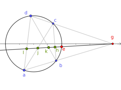
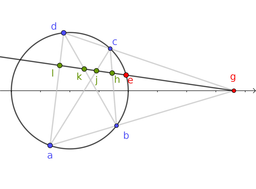
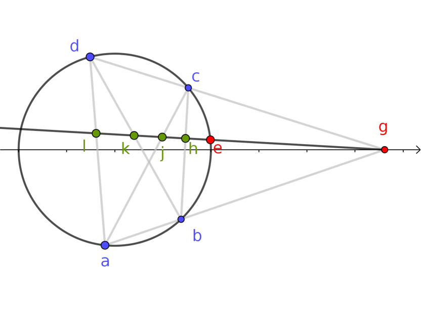
Claim. Let be four complex points on the unit circle in this order so that and are not parallel. Let be an arbitrary point on the Euclidean segment , and fix then , , , and . Note that the special case is possible. Now, (See Figure 1).
Theorem 3.2.
The claim formulated above holds true.
Proof.
Let be a positive real number, and let and be two complex numbers on . Let be the line passing through and :
The intersection points of and are given by the solution of the following equation:
Rearranging terms, we have:
Let be an intersection point different from , i.e.,
Similarly, let
with respect to . Next, take a point on the arc . Let
Then, we have the following (by using Risa/Asir) [FRV, N]:
and
From (2.5) it follows that
| (3.3) |
Using (3.3) we have
and
The proof is completed.
∎
Remark 3.4.
We can see geometrically that the equality holds even if points and are swapped with each other.
4. The Hilbert metric and the visual angle metric of the unit disk
For all distinct points and in a bounded convex domain , the Hilbert metric is defined as [B2, Thm 2.1, p. 157]
| (4.1) |
where , are the intersection points of the line and the domain boundary ordered in such a way that . See the definition of the cross-ratio from (2.1). If , we set . Hilbert [HILB] introduced this metric as an extension of the Klein metric for any bounded convex domain .
Unlike the hyperbolic metric , the Hilbert metric is not invariant under the Möbius automorphisms of as indicated by the following theorem.
Theorem 4.2.
(See [RV, Thm 1.2])) For all , the following functional identity holds between the Hilbert metric and the hyperbolic metric:
where is the Euclidean distance from the origin to the line .
Theorem 4.3.
Under the conditions given in Claim 3.1, the following equalities hold for Hilbert metric:
-
(1)
,
-
(2)
.
Let be a proper subdomain of such that is not a proper subset of a line. The visual angle metric for is defined by
| (4.4) |
That is, the visual angle metric measures the maximal visual angle between the points and at the point on the boundary
Theorem 4.5.
(See [FKV, Thm 1.3]) For , we have
| (4.6) |
where is the absolute value of the midpoint of the chord of the unit disk containing the two points and and hence .
Theorem 4.7.
Under the given conditions in Claim 3.1, the following equalities hold for the visual angle metric:
-
(1)
,
-
(2)
.
The proof of Theorem 4.5 makes use of the inversion mapping the chord onto itself with Under this transformation we also have and, by symmetry, can be easily computed.
Lemma 4.8.
For , the Hilbert distance is given by , where
Proof.
The equation of the line is given by
Let be the intersection points of the line and the unit circle . So, are the solutions to the quadratic equation
From the relation between the roots and the coefficients of a quadratic equation, we have
| (4.9) |
Then, the exponential of the Hilbert distance is given by
The two elements above are reciprocals of each other. Moreover, we remark that the both values and are real because are collinear. So,
| (4.10) |
Eliminating from (4.10) and (4.9) gives us
| (4.11) |
Note that the above equation has two solutions that are reciprocals of each other. Therefore, the larger one gives . In fact,
Hence, the assertion is obtained. ∎
5. A functional identity for the Hilbert metric
In this section, we apply Theorems 4.2 and 4.5 to prove Theorem 1.1 and apply it to study distortion under quasiregular mappings.
5.1.
We next apply the functional identity of Theorem 1.1 to study distortion under quasiregular mappings. For these mappings we refer the reader to [HKV, LV].
5.5.
Remark 5.7.
Theorem 1.2 is apparently new also for the case of analytic functions. In fact, we are not familiar with any distortion results on analytic functions, expressed in terms of the Hilbert metric.
Corollary 5.8.
Let be a -quasiregular mapping and , and let .
-
(1)
Then
-
(2)
If both and hold, then
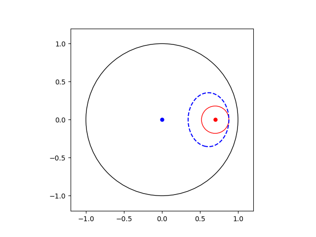
6. Hilbert circles
We consider here Hilbert circles in the unit disk and, in particular, we compare the Hilbert circles to Euclidean circles. We apply Gröbner bases from computer algebra in the same way as in [FRV] to prove that Hilbert circles are Euclidean ellipses.
We first study the defining equation of the Hilbert circle
Theorem 6.1.
For , the boundary of the Hilbert disk forms the ellipse defined by the equation
| (6.2) |
where .
Remark 6.3.
If , the equation (6.2) can be written as
| (6.4) |
where . The above equation is also expressed by
| (6.5) |
So, the semi-minor and semi-major axes are
respectively.
Proof.
For with , the equation of the line passing through the points is given by
| (6.6) |
Let and be the two distinct intersection points of the unit circle and the line with . Since and are points on the unit circle, they are the roots to the following equation, obtained by the substitution into (6.6),
From the relation between the roots and the coefficients of a quadratic equation, we obtain
| (6.7) |
By the definition (4.1)
Since and , setting , we have
| (6.8) |
Using Risa/Asir, a symbolic computation system, eliminating from the system of equation obtained from (6.7) and (6.8), substituting , we obtain
| (6.9) |
where
| (6.10) | ||||
| (6.11) | ||||
(In fact, to find the elimination ideal generated from (6.9), we compute the Gröbner basis of the ideals generated by the polynomials (6.7) and (6.8). For more details see Remark 6.13.)
The first factor of the left side of (6.9) is non-zero because .
Next, for each fixed , we check that the equation defines a curve that is not contained in the unit disk. By rotational symmetry, we may assume . Then, setting , is written as
If , we have
Simplifying the left side, we have
However, the above is not valid as . Therefore, the curve defined by is outside the unit disk and cannot be the Hilbert circle.
On the other hand, we can use the same argument as before to check that the equation defines a curve contained in the unit disk. Setting , is written as
If , we have
Simplifying the left side, we have
But, the above is not valid as . Therefore, the curve defined by is inside the unit disk. Hence, the equation gives a defining equation of the required Hilbert circle. ∎
Remark 6.12.
In fact, from
we can check that is an equation of an ellipse.
Remark 6.13.
Let be the ideal generated by polynomials
and
in variables , and . Computing the Gröbner basis with respect to the box order
we obtain an elimination ideal generated by polynomials in variables and .
The calculation using Risa/Asir shows that the elimination ideal is generated only from the polynomial in the equation (6.9).
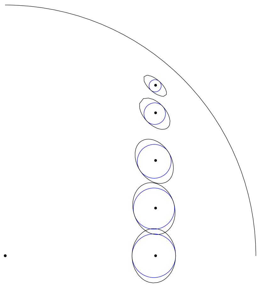
Theorem 6.14.
For and , the following hold.
-
(1)
The largest number satisfying
is , see Figure 5.
-
(2)
The smallest number satisfying
is given by
where and .
Proof.
By (2.7) the hyperbolic circle coincides with the Euclidean circle with the radius and the center at , where
Here, we consider the Hilbert circle and the hyperbolic circle . The equations of these curves are given by,
| (6.15) |
and
| (6.16) |
where and .
We need to find the conditions that the Hilbert circle and the hyperbolic circle are tangent to each other.
First, eliminating from and by computing the resultant, we obtain
In fact, the coefficients of the polynomial are
Next, to find the condition that the equation has multiple solutions, we compute the resultant again,
In fact,
Since , and , the last two factors are significant.
-
•
In the case that , we have
Since , we have . In this case, is inscribed in and we have the assertion of item (1).
-
•
In the case of , we have
In this case, is circumscribed about and we have the assertion of item (2).
∎
It follows from Theorem 4.2 that for , we have
| (6.17) |
and we see that for
| (6.18) |
This inclusion relation is illustrated in Figure 5.
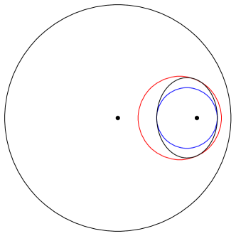
In the case of a Euclidean circle, we have for ,
| (6.19) |
and this is again sharp.
6.20.
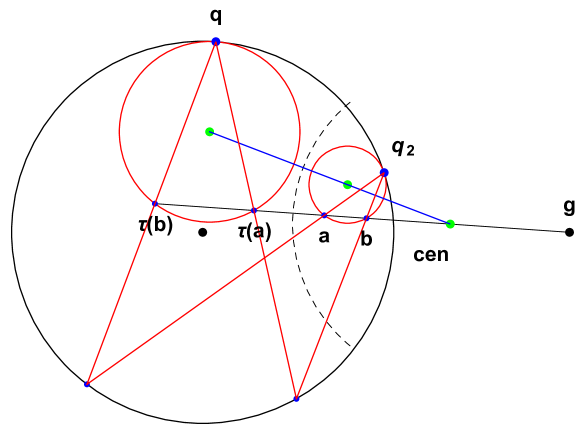
Hilbert midpoint. For the Hilbert midpoint is a point of the form with
Theorem 6.21.
For the Hilbert midpoint is
Moreover,
Proof.
Let and be the points of intersection of the line with the unit circle ordered in such a way that By the definition of the midpoint or, in other words,
Then
| (6.22) |
Hence and are the solution of
Therefore,
| (6.23) |
Eliminating from (6.22), we have the desired value of
The claim about the hyperbolic metric follows readily from the definition of the Hilbert metric. ∎
There are also geometric methods to construct the Hilbert midpoint. We refer the reader to [VW, Fig. 10].
Lemma 6.24.
For
Equality holds if
Proof.
Let be the Hilbert midpoint of and and Then From the formula 6.3 for the major semi-axis of the ellipse we see that decreases as a function of and hence
Because by Theorem 4.2 and (2.7), we have
The sharpness follows from the formula for the hyperbolic metric.
∎
Clearly, convex domains are preserved under affine mappings. It is well-known that the Hilbert metric is preserved under affine mappings. According to Theorem 6.1 we may conclude that Hilbert disks in ellipses are also ellipses.
References
- [B] A. F. Beardon, The Geometry of Discrete Groups, Springer-Verlag, New York, 1983.
- [B2] A. F. Beardon, The Klein, Hilbert, and Poincaré metrics of a domain, J. Comput. Appl. Math., 105 (1999), 155-162.
- [DHV] O. Dovgoshey, P. Hariri, and M. Vuorinen, Comparison theorems for hyperbolic type metrics, Complex Var. Elliptic Equ. 61, 11, (2016), 1464–1480.
- [FKV] M. Fujimura, R. Kargar, and M. Vuorinen, Formulas for the visual angle metric, J. Geom. Anal. arXiv:2304.04485.
- [FRV] M. Fujimura, O. Rainio, and M. Vuorinen, Collinearity of points on Poincaré unit disk and Riemann sphere, Publ. Math. Debrecen 105 (2024) 1-2, 141–169, arXiv:2212.09037.
- [GH] F.W. Gehring and K. Hag, The Ubiquitous Quasidisk. With contributions by Ole Jacob Broch. American Mathematical Society, Providence, RI, 2012. xii+171 pp.
- [HKV] P. Hariri, R. Klén, and M. Vuorinen, Conformally Invariant Metrics and Quasiconformal Mappings, Springer Monographs in Mathematics, Springer, Berlin, 2020.
- [HIMPS] P.A. Hästö, Z. Ibragimov, D. Minda, S. Ponnusamy, and S. Sahoo, Isometries of some hyperbolic-type path metrics, and the hyperbolic medial axis. (English summary) In the tradition of Ahlfors-Bers. IV, 63–74, Contemp. Math., 432, Amer. Math. Soc., Providence, RI, 2007.
- [H] J. Heinonen, Lectures on Analysis on Metric Spaces. Springer-Verlag, New York, 2001.
- [HILB] D. Hilbert, Ueber die gerade Linie als kürzeste Verbindung zweier Punkte, Math. Ann. 46 (1895), 91-96.
- [LV] O. Lehto and K. I. Virtanen, Quasiconformal mappings in the plane. Second edition. Translated from the German by K. W. Lucas. Die Grundlehren der mathematischen Wissenschaften, Band 126. Springer–Verlag, New York–Heidelberg, 1973.
- [N] M. Noro, A computer algebra system Risa/Asir.
- [P] A. Papadopoulos, Metric spaces, convexity and non-positive curvature. Second edition. IRMA Lectures in Mathematics and Theoretical Physics, 6. European Mathematical Society (EMS), Zürich, 2014. xii+309 pp.
- [PT] A. Papadopoulos and M. Troyanov, From Funk to Hilbert geometry. Handbook of Hilbert geometry, 33–67, IRMA Lect. Math. Theor. Phys., 22, Eur. Math. Soc., Zürich, 2014.
- [PY1] A. Papadopoulos and S. Yamada, The Funk and Hilbert geometries for spaces of constant curvature. Monatsh. Math. 172 (2013), no. 1, 97–120.
- [PY2] A. Papadopoulos and S. Yamada, Funk and Hilbert geometries in spaces of constant curvature. Handbook of Hilbert geometry, 353–379, IRMA Lect. Math. Theor. Phys., 22, Eur. Math. Soc., Zürich, 2014.
- [RV] O. Rainio and M. Vuorinen, Hilbert metric in the unit ball, Studia Sci. Math. Hungar. 60(2-3), 2023, 175-191.
- [VW] M. Vuorinen and G. Wang, Bisection of geodesic segments in hyperbolic geometry, Complex Analysis and Dynamical Systems V, Contemp. Math., Israel Math. Conf. Proc., Amer. Math. Soc., Providence, RI. 591, 2013, 273–290.