Microscopic investigation of $E2$ matrix elements in atomic nuclei

Abstract

A systematic analysis of $E2$ matrix elements of ⁷²Ge, ⁷⁶Ge, ¹⁶⁸Er, ¹⁸⁶Os, ¹⁸⁸Os, ¹⁹⁰Os, ¹⁹²Os and ¹⁹⁴Pt nuclides is performed using the beyond mean-field approach of triaxial projected shell model (TPSM). For these nuclei, large sets of $E2$ matrix elements have been deduced from the multi-step Coulomb excitation experiments, and it is shown that TPSM approach provides a reasonable description of the measured transitions. We have evaluated 1496 $E2$ matrix elements up to spin, $I=10$ for the eight nuclei studied, and tabulate them for future experimental and theoretical comparisons. Further, shape invariant analysis has been performed with the calculated $E2$ transitions using the Kumar-Cline sum rules. It is inferred from the analysis that the resulting shape, after configuration mixing of the quasiparticle states, transforms from $\gamma$-rigid to that of $\gamma$-soft for some nuclei, in conformity with the experimental data.

I Introduction

The Coulomb excitation (COULEX) mechanism provides an invaluable information on the $E2$ matrix elements of the nuclear states [1]. In the early days of nuclear physics, it was possible to populate only low-spin states with light-ion beams. However, the availability of the heavy-ion beams coupled with the development of the high-resolution gamma-ray detector arrays has led to a renaissance in the field of COULEX. Further, very advanced computer codes, for instance, GOSIA [2] have been developed for analysing the vast amounts of data collected from these advanced COULEX experiments. It is now possible to extract a complete set of $E2$ matrix elements for low-lying states up to an excitation energy of 2 MeV from the COULEX data.

The extraction of a large set of $E2$ matrix elements for a given nucleus has made it possible to infer the shape of the nucleus in a model independent way by calculating the quadrupole shape invariants [1]. It is known that electric quadrupole spherical tensor operators can be expressed as products of rotationally invariant quantities, which can then be related to the ellipsoidal charge distribution of the nucleus in the intrinsic frame of reference [3]. The product of two- and three operators can be written in terms of ellipsoidal shape parameters, similar to $\beta$ and $\gamma$ parameters of Bohr-Mottelson collective model [4]. The expectation values of the products of quadrupole operators can be completely expressed in terms of $E2$ matrix elements of intermediate states involved in the summation. This method of evaluating the rotational invariant quantities from measured $E2$ matrix elements provides a direct measure of the shape of the equivalent ellipsoid in the intrinsic frame. In Bohr-Mottelson collective model, rotational $D$-functions are employed to transform the quantities to the laboratory frame [4].

Detailed $E2$ matrix elements have been deduced from COULEX experiments in several regions of the mass table [5, 6, 1, 7, 8, 9]. In the mass $A\sim 160$ region ¹⁶⁸Er is probably one of the best studied systems with about 50 $E2$ matrix elements known for the yrast- and the $\gamma$-bands [5]. The COULEX experiments on shape transitional Pt-Os region with $A\sim 190$ extracted $E2$ matrix elements for several of these isotopes up to $I=12$ [7, 1]. In the medium mass region, $A\sim 100$, extended sets of $E2$ and $M1$ matrix elements in ¹⁰⁴Ru, ⁷²Ge and ⁷⁶Ge have been measured by means of COULEX [6, 9, 10, 8].

The evaluated $E2$ matrix elements have been compared with the two extreme limits of the Bohr-Mottelson collective Hamiltonian, the rigid asymmetric rotor [11] and the $\gamma$-independent potential energy [12]. Further, the interacting boson model (IBM), with the Hamiltonian fitted to the energy spectra, has also been employed to investigate the measured $E2$ matrix elements [13, 14, 15]. It has been shown that these three purely phenomenological approaches reproduce only some aspects of the known COULEX data [6, 5, 1, 10, 7, 16, 9, 8, 17, 18].

The availability of the extended sets of $E2$ matrix elements represent a benchmark for assessing the validity and scope of the microscopic approaches to describe the dynamics of the collective quadrupole degrees of freedom. Several nuclear structure models with some microscopic features have been developed and here we only mention the microscopic Bohr Hamiltonian derived from quadrupole-quadrupole interaction, what is referred to as the quadrupole constrained Bohr Hamiltonian (QCBH) [19]. This model has been used to describe the COULEX $E2$ matrix elements for several nuclides with varying success [5, 6, 7, 8, 9].

The purpose of the present work is to employ the large sets of E2 matrix elements for eight nuclides, available from the COULEX data, as benchmarks to appraise the performance of the beyond mean-field microscopic approach of the triaxial projected shell model (TPSM), which extends our earlier detailed study on ¹⁰⁴Ru along these lines [20]. In contrast to microscopic versions of the Bohr Hamiltonian, the TPSM approach does not introduce an explicit ansatz for the collective quadrupole degrees of freedom, and avoids invoking the adiabatic approximation. The model rather represents a shell model based approach with angular momentum projected deformed configurations as the basis states. The deformed states contain essential correlations needed to describe the deformed systems, and the collective features emerge directly from the microscopic degrees of freedom. As this approach includes multi-quasiparticle configurations, it is capable of describing the properties of nuclei up to quite high-spin. In several studies, it has been shown that TPSM approach provides a remarkable description of the single-particle and collective excitations in deformed and transitional systems [21, 22, 23]. The phenomena of chiral symmetry and wobbling motion have been investigated in detail in the TPSM approach [22]. Recently, a systematic study of the $\gamma$-bands observed in atomic nuclei have been undertaken, and it has been shown that staggering phase of these bands can change from the pattern of $\gamma$-rigid to that of $\gamma$-soft with the inclusion of the quasiparticle excitations [23, 24].

In our more recent work [20], we calculated a complete set of $E2$ matrix elements, the centroids and dispersions of the shape invariants for ¹⁰⁴Ru were investigated. Our work demonstrated that, although the triaxial mean-field in the TPSM approach is $\gamma$-rigid, the beyond-mean-field procedure of admixing angular-momentum projected multi-quasiparticle states to the projected vacuum configuration alters the characteristics of ¹⁰⁴Ru from $\gamma$-rigid to $\gamma$-soft as deduced from the measured $E2$ matrix elements. In the present manuscript, the analysis carried out for ¹⁰⁴Ru is broadened for the eight nuclei of ⁷²Ge, ⁷⁶Ge, ¹⁶⁸Er, ¹⁸⁶Os, ¹⁸⁸Os, ¹⁹⁰Os, ¹⁹²Os and ¹⁹⁴Pt. We have chosen these systems as extensive $E2$ matrix elements have been measured for these systems [5, 6, 7, 9, 10]. The remaining manuscript is organized in the following manner. The TPSM approach and shape invariant sum rule analysis are briefly discussed for completeness in sections II and III respectively. In section IV, the results of $E2$ matrix elements and shape invariant quantities are presented and compared with the known data [5, 6, 7]. In section V, the present work is summarized and concluded.

II Triaxial Projected Shell Model Approach

TPSM approach has its roots in the pairing plus quadrupole model (PPQM) of Kumar and Baranger [25]. PPQM is the microscopic formulation of the well-known collective model of Bohr and Mottelson (BM) with quadrupole and pairing degrees of freedom as the basic building blocks [4]. There have been several studies demonstrating that low-lying properties of atomic nuclei can be described reasonably well using the PPQM approach [26]. In the seventies and eighties, high-spin properties of rotating nuclei were systematically investigated using the PPQM Hamiltonian by applying the cranking [27] and angular-momentum projection techniques [28]. However, most of these studies were restricted to investigate the properties of rotating nuclei close to the yrast configuration [29]. In the deformed $A\sim 160$ region, more than twenty side-bands have been identified in some nuclei and in order to elucidate the properties of these rich band structures, it is imperative to include quasiparticle excited configurations in the model. The semiclassical cranked shell model (CSM) [30] introduced the concept of quasiparticles in a rotating potential, which allowed the authors to classify the complex band structures as independent quasiparticle configurations of these building blocks. However, in this approach, the quasiparticle states don’t have well defined angular-momentum and predictions of transition probabilities become less reliable, in particular for interband transitions.

In an attempt to investigate the rich band structures observed in deformed nuclei, projected shell model (PSM) approach has been developed [28]. In this approach, the multi-quasiparticle configurations are generated from deformed Nilsson potential and the Bardeen-Cooper-Schriffer (BCS) approximation. The Nilsson potential is directly employed as the quadrupole mean-field instead of solving the Hartree-Fock (HF) equation with quadrupole-quadrupole interaction [28]. This approach has the advantage that the Nilsson parameters have been fitted to a large set of the experimental data, and is known to provide an accurate description of the ground state properties of deformed nuclei [31, 32]. The deformed Nilsson basis is then employed to construct the multi-quasiparticle states with the use of the BCS formalism. In the second step, the quasiparticle configurations are projected onto good angular-momentum states using the angular-momentum projection operator [28]. In the final stage, the projected states are used to diagonalize the shell model Hamiltonian consisting of pairing (monopole and quadrupole) and quadrupole-quadrupole interaction terms. This approach is similar to the spherical shell model (SSM) approach with the difference that deformed basis is used in comparison to the spherical basis used in SSM. The deformed basis constitute the optimum basis to investigate a deformed system, and the TPSM analysis needs only about 60 quasiparticle states to describe a deformed nucleus up to quite high-spin.

In the original version of the projected shell model approach [33, 34, 35, 36, 37, 38], the deformed basis were restricted to have axial symmetry and transitional nuclei could not be studied using this approach. The model was generalized to include triaxial basis states, which are obtained by solving the three dimensional Nilsson potential [21]. This extended version of the model, what is referred to as the TPSM approach, has been shown to describe the properties of transitional nuclei remarkably well [21, 22, 23, 39] and the reason is that the TPSM incorporates the collective features caused by deviations from axial shape.

In the present work, we have used the extended TPSM version [21, 22, 23, 39] to investigate the detailed $E2$ matrix of even-even isotopes. The projected basis states considered for studying the even-even system are the vacuum, the two-proton, the two-neutron and the two-proton plus two-neutron quasiparticle configurations, i.e.,

$$\{\hat{P}^{I}_{MK}\left|\Phi\right>,~\hat{P}^{I}_{MK}~a^{\dagger}_{p_{1}}a^{\dagger}_{p_{2}}\left|\Phi\right>,~\hat{P}^{I}_{MK}~a^{\dagger}_{n_{1}}a^{\dagger}_{n_{2}}\left|\Phi\right>,$$

$$~\hat{P}^{I}_{MK}~a^{\dagger}_{p_{1}}a^{\dagger}_{p_{2}}a^{\dagger}_{n_{1}}a^{\dagger}_{n_{2}}\left|\Phi\right>\},$$ (1)

where $\left|\Phi\right>$ in (1) represents the triaxial quasiparticle vacuum state. In majority of the nuclei, near-yrast spectroscopy up to $I=20$ is well described using the above basis space.

The quasiparticle states are the standard BCS ones for the single particle states of the Nilsson Hamiltonian [40],

$$\hat{H}_{N}=\hat{H}_{0}-{2\over 3}\hbar\omega\left\{\epsilon\hat{Q}_{0}+\epsilon^{\prime}{{\hat{Q}_{+2}+\hat{Q}_{-2}}\over\sqrt{2}}\right\}.$$ (2)

The term $\hat{H}_{0}$ contains the spherical single-particle energies, the parameters of which are fitted to a broad range of nuclear properties [28]. The axial deformation parameter $\varepsilon$ and triaxiality parameter $\varepsilon^{\prime}$ (or $\gamma=\arctan(\varepsilon^{\prime}/\varepsilon$) are fixed input parameters of the model. They are adjusted to reproduce the reduced transition probability $B(E2,2^{+}_{1}\rightarrow 0^{+}_{1})$ and the energy $E(2^{+}_{2})$ of the $\gamma$-band head. Table 1 provides these parameters for the nuclides studied in the present work.

The basis (1) is employed to diagonalize the TPSM Hamiltonian, which consists of pairing and quadrupole-quadrupole interaction terms, i.e.,

$$\hat{H}=\hat{H}_{0}-{1\over 2}\chi\sum_{\mu}\hat{Q}^{\dagger}_{\mu}\hat{Q}_{\mu}-G_{M}\hat{P}^{\dagger}\hat{P}-G_{Q}\sum_{\mu}\hat{P}^{\dagger}_{\mu}\hat{P}_{\mu}.$$ (3)

The QQ-force strength, $\chi$, in Eq. (3) is determined from the quadrupole deformation $\epsilon$ as a result of the self-consistency HFB condition [28]:

$$\chi_{\tau\tau^{\prime}}={{{2\over 3}\epsilon\hbar\omega_{\tau}\hbar\omega_{\tau^{\prime}}}\over{\hbar\omega_{n}\left<\hat{Q}_{0}\right>_{n}+\hbar\omega_{p}\left<\hat{Q}_{0}\right>_{p}}},$$ (4)

where $\omega_{\tau}=\omega_{0}a_{\tau}$, with $\hbar\omega_{0}=41.4678A^{-{1\over 3}}$ MeV, and the isospin-dependence factor $a_{\tau}$ is defined as

$$a_{\tau}=\left[1\pm{{N-Z}\over A}\right]^{1\over 3},$$ (5)

with $+$ $(-)$ for $\tau=$ neutron (proton). The harmonic oscillation parameter is given by $b^{2}_{\tau}=b^{2}_{0}/a_{\tau}$ with $b^{2}_{0}=\hbar/{(m\omega_{0})}=A^{1\over 3}$ fm². Note that the strengths in the TPSM are fixed as in the original PSM with axial symmetry [28]. Possible corrections from the non-axial component of the quadrupole field have been neglected in the present work.

Table 1: Axial and triaxial quadrupole deformation parameters $\epsilon$ and $\epsilon^{\prime}$ employed in the TPSM calculation. Axial deformations are taken from our earlier works [23, 41, 42, 43, 44] and [45], and nonaxial deformations are chosen in such a way that heads of the $\gamma$-bands are reproduced.

Isotope	72Ge	76Ge	168Er	186Os	188Os	190Os	192Os	194Pt
$\epsilon$	0.230	0.200	0.321	0.200	0.183	0.178	0.164	0.125
$\epsilon^{\prime}$	0.160	0.160	0.130	0.118	0.088	0.092	0.085	0.073

The monopole pairing strength $G_{M}$ (in MeV) is of the standard form

$$G_{M}={{G_{1}\mp G_{2}{{N-Z}\over A}}\over A},$$ (6)

where the minus (plus) sign applies to neutrons (protons). In the present calculation, we choose $G_{1}$ and $G_{2}$ such that the calculated gap parameters reproduce the experimental mass differences. The values $G_{1}$ and $G_{2}$ vary depending on the mass region and shall be listed in the discussion of the results. The above choice of $G_{M}$ is appropriate for the single-particle space employed in the model, where three major shells are used for each type of nucleon. For most of the nuclei, Eq. (6) has been employed. However, it has been found that for protons, $G_{M}={G_{1}\over A}$ reproduces the pairing gaps for $A\sim 130$ region [46] slightly better and has been employed in this region. The quadrupole pairing strength $G_{Q}$ is considered to be proportional to $G_{M}$ and the proportionality constant being fixed as 0.18. These interaction strengths are consistent with those used in our earlier studies [42, 47, 48, 49, 50, 51, 28, 52, 53, 38, 54, 55].

The projection formalism outlined above can be transformed into a diagonalization problem following the Hill-Wheeler prescription. The Hamiltonian in Eq. (3) is diagonalized using the projected basis of Eq. (1). The obtained wavefunction can be written as

$$\psi^{\sigma I}_{IM}=\sum_{K,\kappa}f^{\sigma}_{\kappa K}\hat{P}^{I}_{MK}|~\Phi_{\kappa}\rangle$$ (7)

Here, the index ${}^{``}\sigma^{"}$ labels the eigenstates for a given angular momentum and ${}^{``}\kappa^{"}$ the quasiparticle configurations of the basis states. In Eq. (7), $f^{\sigma}_{\kappa K}$ are the amplitudes of the basis states $\kappa,K$. These wavefunctions are used to calculate matrix element of a multipole operator $\hat{\mathcal{O}}_{L}$ given by

$$\langle\psi^{\sigma_{f}}_{I_{f}M_{f}}|\hat{\mathcal{O}}_{LM} |\psi^{\sigma_{i}}_{I_{i}M_{i}}\rangle$$

$$=(I_{i}M_{i},LM|I_{f}M_{f})\langle\sigma_{f},I_{f}||\hat{\mathcal{O}}_{L}||\sigma_{i},I_{i}\rangle,$$ (8)

where the reduced matrix element of an operator $\hat{\mathcal{O}}$ can be expressed as [56]

$$\langle\sigma_{f},I_{f}||\hat{\mathcal{O}}_{\lambda} ||\sigma_{i},I_{i}\rangle$$

$$=\sum_{\kappa_{i},K_{i},\kappa_{f},Kf}{f_{\kappa_{i}K_{i}}^{\sigma_{i}I_{i}}}~~~{f_{\kappa_{f}K_{f}}^{\sigma_{f}I_{i}}}\sum_{M_{i},M_{f},M}(-)^{I_{f}-M_{f}}$$

$$~~~~~~~\times\left(\begin{array}[]{ccc}I_{f}&L&I_{i}\\ -M_{f}&M&M_{i}\end{array}\right)$$ (11)

$$~~~~~~~\times\langle\Phi_{\kappa_{f}}|{\hat{P}^{I_{f}}}_{K_{f}M_{f}}\hat{\mathcal{O}}_{LM}\hat{P}^{I_{i}}_{K_{i}M_{i}}|\Phi_{\kappa_{i}}\rangle$$

$$=2\sum_{\kappa_{i},\kappa_{f}}{f_{\kappa_{i}K_{i}}^{\sigma_{i}I_{i}}}~~~{f_{\kappa_{f}K_{f}}^{\sigma_{f}I_{f}}}\sum_{M^{\prime},M^{\prime\prime}}(-)^{I_{f}-K_{\kappa_{f}}}{(2I_{f}+1)}^{-1}$$

$$~~~~~~~\times\left(\begin{array}[]{ccc}I_{f}&L&I_{i}\\ -K_{f}&M^{\prime}&M^{\prime\prime}\end{array}\right)~\int d\Omega\,D^{I_{i}}_{M^{\prime\prime}K_{i}}(\Omega)$$ (14)

$$~~~~~~~\times\langle\Phi_{\kappa_{f}}|\hat{\mathcal{O}}_{LM^{\prime}}\hat{R}(\Omega)|\Phi_{\kappa_{i}}\rangle.$$ (15)

III Invariant Sum Rule Analysis

The individual $E2$ matrix elements are strongly correlated by the quadrupole collectivity, and the number of important collective variables is substantially lower than the number of matrix elements [1]. The conventional method of comparing the TPSM results to the set of experimental $E2$ matrix elements demonstrates the capability of the model to account for the data. The projection of the collective characteristics from both the data and the microscopic calculations provides a greater insight. Following the work of Kumar and Cline, the experimental electromagnetic matrix elements can be interpreted in terms of collective degrees of freedom for any state by using the expectation values of rotationally invariant products of multipole operators which relate properties in the principal axis frame to those in the laboratory frame[1, 3].

The spherical tensor nature of electromagnetic multipole operators makes it possible to construct zero-coupled products of such operators that are rotationally invariant. This implies that in the intrinsic frame and the laboratory frame, these products are identical. For simplicity consider the case of the electric quadrupole operator $E2$. The intrinsic principal axis frame electric moments can be described in terms of two parameters ($Q,\delta$) by analogy with Bohr’s shape parameters ($\beta,\gamma$) as

$$E(2,0)=Q\textrm{cos}\delta$$

$$E(2,1)=E(2,-1)=0$$ (16)

$$E(2,2)=E(2,-2)=\frac{1}{\sqrt{2}}.Q\textrm{sin}\delta$$

where $Q$ and $\delta$ are the arbitrary parameters and $Q$ can be written in terms of intrinsic quadrupole moment for an axially symmetric shape as $Q=\sqrt{\frac{5}{16\pi}}Q_{0}$. In terms of the principal axis frame parameters, zero coupled products of $E2$ operators can be written as

$$[E2\times E2]^{0}=\frac{1}{\sqrt{5}}Q^{2}$$

$$\left[[E2\times E2]^{2}\times E2\right]^{0}=-\sqrt{\frac{2}{35}}Q^{3}\textrm{cos}3\delta.$$ (17)

The symbol $[...\times...]^{L}$ stands for vector coupling to angular momentum $L$. The coefficients in front of $Q^{2}$ and $Q^{3}$ are the corresponding products of the Wigner symbols. In order to have a correspondence with collective coordinates, these invariants are denoted here up to coefficients as $Q^{2}$ and $Q^{3}\textrm{cos}3\delta$. The expectation values of the $E2$ rotation invariants in the laboratory frame can be related to the reduced $E2$ matrix elements by making intermediate state expansions. The corresponding sum rules read:

$$\langle S| [E2\times E2]^{0}|S\rangle$$

$$=\frac{(-)^{2S}}{\sqrt{2S+1}}\sum_{R}\langle S||E2||R\rangle\langle R||E2||S\rangle\left\{\begin{array}[]{ccc}2&2&0\\ S&S&R\end{array}\right\}$$ (20)

$$\langle S|[[ E2\times E2]^{2}\times E2]^{0}|S\rangle$$

$$=\sqrt{\frac{5}{2S+1}}\sum_{RT}\langle S||E2||R\rangle\langle R||E2||T\rangle\langle T||E2||S\rangle$$

$$~~~~~~~~~~\times\left\{\begin{array}[]{ccc}2&2&0\\ S&S&T\end{array}\right\}\left\{\begin{array}[]{ccc}2&2&2\\ T&S&R\end{array}\right\}(-)^{3S+T}$$ (25)

where $S$ denotes state $S$ and at the same time the spin of state $S$ alone, $R$ and $T$ denotes the intermediate states and their spins, and $\{~~~~~~\}$ represents the $6j$ symbol. These intermediate states allows the rotational invariants built from $Q$ and $\delta$ to be expressed as the sums of the products of the reduced $E2$ matrix elements using the experimental data of these matrix elements with proper relative signs and magnitudes. This will directly determine the quantum distribution i.e., the centroids, dispersions, skewnesses, cross-correlation coefficients, etc., of $E2$ in a given state. The invariant $\langle S|Q^{2}|S\rangle$, i.e., expectation value of $Q^{2}$, denoted simply as $\langle Q^{2}\rangle$ is given by

$$\langle Q^{2}\rangle=\frac{1}{2S+1}\sum_{R}|\langle S||E2||R\rangle|^{2}$$ (26)

The invariant $\langle Q^{2}\rangle$ does not depend upon the sign of any matrix element, in contrast to invariant $\langle Q^{3}\textrm{cos}3\delta\rangle$ which is given by

$$\langle Q^{3} \textrm{cos}3\delta\rangle$$

$$=\mp\sqrt{\frac{35}{2}}\frac{1}{2S+1}\sum_{RT}\langle S||E2||R\rangle\langle R||E2||T\rangle\langle T||E2||S\rangle$$

$$~~~~~~~~~~~~~~~~~~~~~~~~~~~~~~~~~~~~~\times\left\{\begin{array}[]{ccc}2&2&2\\ S&T&R\end{array}\right\}$$ (29)

where positive and negative signs correspond to integral and half-integral spin system respectively.

The dispersion of $Q^{2}$ is given by

$$\sigma(Q^{2})=\sqrt{\langle Q^{4}\rangle-\langle Q^{2}\rangle^{2}}$$ (30)

and the dispersion of the quadrupole asymmetry is given by

$$\sigma(\textrm{cos}3\delta)=\left[\frac{\langle\left(Q^{3}\textrm{cos}3\delta\right)^{2}\rangle}{\langle Q^{6}\rangle}-\left(\frac{\langle Q^{3}\textrm{cos}3\delta\rangle}{\langle Q^{2}\rangle^{3/2}}\right)^{2}\right]^{1/2}$$ (31)

The calculation of the dispersions requires the evaluation of the higher order tensor products $\langle Q^{4}\rangle$,$\langle Q^{6}\rangle$ and $\langle\left(Q^{3}\textrm{cos}3\delta\right)^{2}\rangle$. In analogy to Eqs. (26) - (III), they are evaluated by multiple intermediate sums, the pertaining expression of which are given in Ref. [1]. The sums involve an increasing number of $E2$ matrix elements, the limit being set by the practical feasibility.

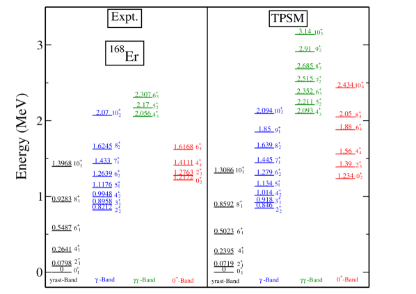
Figure 1: (Color online) TPSM and experimental energies of the lowest bands in ¹⁶⁸Er. The states are labelled by $I^{+}_{n}$. These labels are used in the figures and tables to identify the states.

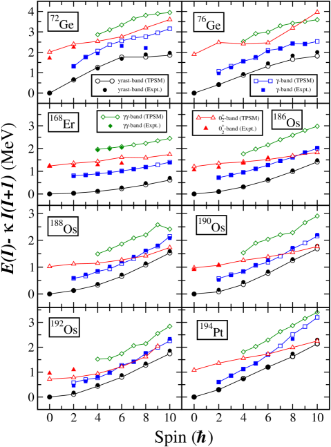
Figure 2: (Color online) TPSM and experimental energies of the yrast-, $\gamma$-, $\gamma\gamma$- and $0_{2}^{+}$-bands of ^72,76Ge, ¹⁶⁸Er,^{186,188,190,192}Os and ¹⁹⁴Pt isotopes. The scaling factor $\kappa=32.32A^{-5/3}$.

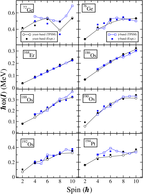
Figure 3: (Color online) TPSM and experimental $\hbar\omega(I)$ values of the yrast- and $\gamma$-bands of ^72,76Ge, ¹⁶⁸Er,^{186,188,190,192}Os and ¹⁹⁴Pt isotopes. Note that the experimental symbols cover the TPSM symbols.

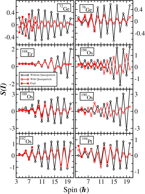
Figure 4: (Color online) Staggering parameters $S(I)$ of the $\gamma$-band in ^72,76Ge, ¹⁶⁸Er,^{186,188,190,192}Os and ¹⁹⁴Pt.

IV Results and Discussion

In this section, we shall present and discuss the TPSM results for the eight nuclides of ⁷²Ge, ⁷⁶Ge, ¹⁶⁸Er, ¹⁸⁶Os, ¹⁸⁸Os, ¹⁹⁰Os, ¹⁹²Os and ¹⁹⁴Pt. We have evaluated both excitation energies and the $E2$ matrix elements, which are presented in the following two subsections. In the third subsection, the analysis of the quadrupole shape invariants is discussed.

IV.1 Excitation Energies

The primary objective of the present work is to investigate the $E2$ matrix elements. However, before discussing these quantities, we shall first demonstrate that the TPSM approach reproduces the excitation energies reasonably well for the eight nuclides studied. As an illustrative example to demonstrate the robustness of the TPSM approach, Fig. 1 compares the experimental level energies of the lowest four positive parity bands in ¹⁶⁸Er with the TPSM predictions. The results are depicted only for the low-lying states of the four bands that are populated in the COULEX experiments. The band based on the $2^{+}_{2}$ is the $\gamma$-band. Its energy is adjusted to the experimental value by choosing the appropriate value of the input triaxial parameter, $\varepsilon^{\prime}$. The band based on the $4^{+}_{3}$ level is called the $\gamma\gamma$-band throughout the paper. However, it needs to be added that it may be only a fragment of the collective double $\gamma$ vibration due to its coupling with two-particle excitations. The TPSM approach accounts for the fragmentation which will be discussed in detail in a separate work.

The excited $0^{+}$-band with band head labeled as $0^{+}_{2}$ is higher in energy than the $\gamma$-band. For some nuclides studied here, the excited $0^{+}$-band crosses the $\gamma$-band. However, irrespective of the position of the states, we shall follow the labeling used in Fig. 1 throughout the manuscript. For instance, $6^{+}_{4}$ will always correspond to the excited $0^{+}$-band.

For a detailed comparison between the experimental and TPSM energies, Fig. 2 displays the excitation energies for all eight studied nuclei with a common reference energy subtracted in order to expand the energy scale of the curves. Evidently, the TPSM reproduces the energies of the yrast- and $\gamma$-bands quite well. The energies of $\gamma\gamma$- and $0^{+}_{2}$-bands are also reasonably well described for the known states. However, the data is insufficient for these bands for a thorough comparison. A comprehensive comparison for more than 30 nuclides can be found in our previous studies [23, 24].

To probe the rotational properties of the systems, Fig. 3 compares the empirical rotational frequencies, defined as,

$$\hbar\omega(I)=\frac{E(I)-E(I-2)}{2}$$ (32)

with the corresponding TPSM values. Both the yrast- and the $\gamma$-band frequencies are reproduced very well. The leveling or down-bend of $\hbar\omega(I)$ at high spin is caused by the admixture of a pair of rotationally aligned $i_{13/2}$ quasineutrons in the case of the rare earth nuclei, and a pair of aligned $g_{9/2}$ quasineutrons in the case of the Germanium isotopes.

We have also evaluated the staggering parameter of the $\gamma$-band, defined as,

$$S(I)=\frac{[E(I)-E(I-1)]-[E(I-1)-E(I-2)]}{E(2^{+}_{1})}~~~~,$$ (33)

and displayed it in Fig. 4. The phase of $S(I)$ is used to classify nuclei as "$\gamma$-rigid" when the odd $I$ levels are below the adjacent even $I$ levels or "$\gamma$-soft" when the even $I$ levels are below the odd $I$ states. The classification is based on the concept of the collective Hamiltonian in the $\gamma$ degree of freedom, where "soft" and "rigid" refer to the potential confining the fluctuations of the shape around the mean value. We discussed this classification scheme in detail in Ref. [24]. Accordingly, ⁷²Ge and ¹⁸⁶Os are "$\gamma$-soft" and ⁷⁶Ge, ¹⁹²Os and ¹⁹⁴Pt are "$\gamma$-rigid", while as ¹⁸⁸Os and ¹⁹⁰Os indicate the transitional behaviour between soft- and rigid-motion. ¹⁶⁸Er displays very small $S(I)$ values, which indicate a small deviation from the axial shape.

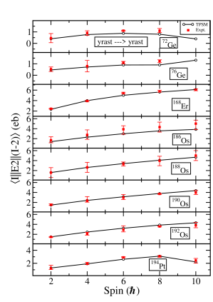
Figure 5: (Color online) Reduced in-band E2 matrix elements for transitions yrast $\rightarrow$ yrast in ^72,76Ge, ¹⁶⁸Er,^{186,188,190,192}Os and ¹⁹⁴Pt. Expt. data is taken from the Refs. [6, 9, 10, 5, 7, 16].

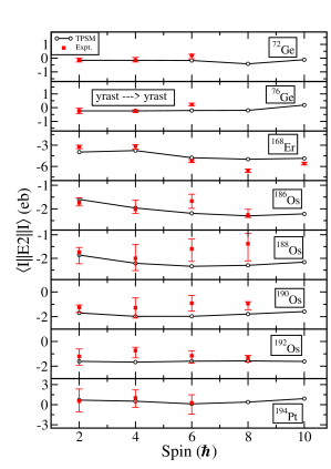
Figure 6: (Color online) Reduced diagonal E2 matrix elements for the yrast states in ^72,76Ge, ¹⁶⁸Er,^{186,188,190,192}Os and ¹⁹⁴Pt. Expt. data is taken from the Refs. [6, 9, 10, 5, 7, 16].

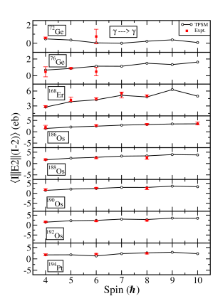
Figure 7: (Color online) Reduced in-band E2 matrix elements for transitions $\gamma$ $\rightarrow$ $\gamma$ in ^72,76Ge, ¹⁶⁸Er,^{186,188,190,192}Os and ¹⁹⁴Pt. Expt. data is taken from the Refs. [6, 9, 10, 5, 7, 16].

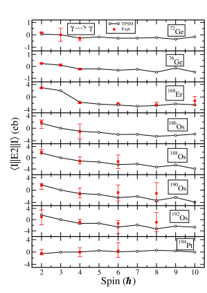
Figure 8: (Color online) Reduced diagonal E2 matrix elements for the $\gamma$-band states ^72,76Ge, ¹⁶⁸Er,^{186,188,190,192}Os and ¹⁹⁴Pt. Expt. data is taken from the Refs. [6, 9, 10, 5, 7, 16].

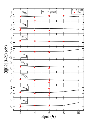
Figure 9: (Color online) Reduced inter-band E2 matrix elements for transitions $\gamma$ $\rightarrow$ yrast in ^72,76Ge, ¹⁶⁸Er,^{186,188,190,192}Os and ¹⁹⁴Pt. Expt. data is taken from the Refs. [6, 9, 10, 5, 7, 16].

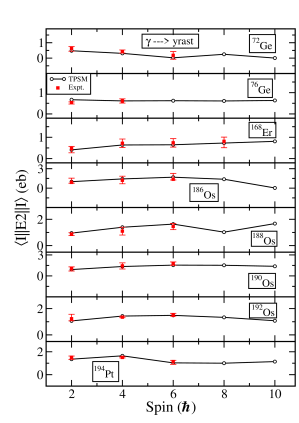
Figure 10: (Color online) Reduced inter-band E2 matrix elements for transitions $\gamma$ $\rightarrow$ yrast in ^72,76Ge, ¹⁶⁸Er,^{186,188,190,192}Os and ¹⁹⁴Pt. Expt. data is taken from the Refs. [6, 9, 10, 5, 7, 16].

IV.2 $E2$ matrix elements

In this section, we provide a detailed comparison of the $E2$ matrix elements for ⁷²Ge, ⁷⁶Ge, ¹⁶⁸Er, ¹⁸⁶Os, ¹⁸⁸Os, ¹⁹⁰Os, ¹⁹²Os and ¹⁹⁴Pt evaluated using the TPSM approach with the available experimental values. These eight nuclides have been chosen because large sets of $E2$ matrix elements have been measured through COULEX experiments. Partial sets of the $E2$ matrix elements for yrast- and $\gamma$-bands are displayed in Figs. 5-10 and all the matrix elements up to $I=10$ for yrast-, $\gamma$- $\gamma\gamma$- and $0_{2}^{+}$-bands are listed in Tables LABEL:E2INBD to LABEL:E2INTERBS3 of the Appendix A. The total number of 1496 tabulated matrix elements listed in the tables should be useful for future experimental and theoretical comparisons. We have limited the evaluation of the matrix elements to $I=10$ as most of the COULEX data are restricted this spin value.

Before proceeding further with the discussion of the matrix elements, we would like to note that there is a partial ambiguity in the signs of the non-diagonal reduced matrix elements because the sign of the eigenvector does not have a physical relevance. It is a matter of the adopted phase convention. Following the standard convention in evaluating the $E2$ matrix elements in COULEX experiments [5, 6, 7, 8], we assign a $+$ sign to all in-band matrix elements $\langle I||E2||I-2\rangle$. Further, one needs to assign the sign of one matrix element $\langle I||E2||I-1\rangle$ between the even and odd-$I$ sequences of the $\gamma$- and $\gamma\gamma$-bands and the sign of one matrix element between the bands. This fixes the signs of the eigenvectors and the signs of the remaining matrix elements. [The situation is analogous to the transition energies. Knowing the in-band transition energies and one transition energy between each band fixes all the transition energies between the bands.] Figs. 5-10 depict the matrix elements with the sign convention of the COULEX experiments. In the event this sign convention required reversing the sign of the matrix element obtained in the TPSM calculations, the original sign is quoted in the parentheses of the matrix element listed in the table.

The reduced $E2$ matrix elements corresponding to the transitions $I\rightarrow I-2$ within the yrast-band are depicted in Fig. 5 and listed in Table LABEL:E2INBS1. According to the adopted phase convention they are positive. The matrix elements exhibit an increasing trend with spin, which is a general feature obtained in most of models [5, 6, 7]. It is evident from the figure that agreement between the TPSM values and the measured matrix elements is quite good.

The diagonal matrix elements of the yrast-bands, which represent the static quadrupole moments, are shown in Fig. 6 and listed in Table LABEL:E2INBD. The signs of these matrix elements do not depend on the phase convention and represent a physical quantity. The TPSM values reproduce the measured matrix elements quite well. As discussed in detail in Ref. [24], the negative values for the yrast states in ¹⁶⁸Er and ^186-192Os indicate a preference for prolate deformation. This is also evident from the change of the sign of the matrix elements from positive to negative for the values of the $\gamma$-band. The small absolute values for ^72,76Ge and ¹⁹⁴Pt are evidence for the triaxiality being close to its maximum, where the negative sign for the Germanium isotopes indicate that the shape is slightly on the prolate side where the moments of inertia, ${\cal J}_{l}<{\cal J}_{s}$. The positive sign for Pt indicates that the shape is slightly on the oblate side where ${\cal J}_{s}<{\cal J}_{l}$. A detailed discussion on the relationship between the moment of inertia and the $E2$ matrix elements is given in Ref. [24].

The stretched in-band $E2$ matrix elements for the $\gamma$-band are depicted in Fig. 7 and displayed in Table LABEL:E2INBS1. They are positive due to the adopted phase convention. For ⁷²Ge, the values are almost constant with spin, and for other nuclides a slightly increasing trend is noted, which is consistent with the experimental data. The small values for ^72,76Ge and ¹⁹⁴Pt are evidences for their strong triaxiality [24].

The TPSM diagonal matrix elements of the $\gamma$-band are shown in Fig. 8 and listed in Table LABEL:E2INBD. For the $I=2^{+}$ and $3^{+}$ states of ¹⁶⁸Er and ^186-192Os they are positive and change to negative values with increasing $I$, which indicates a preference for prolate deformation. The measured values for the known states also display this feature, although in some cases the error bars are too large for a definite comparison. The small absolute values for ^72,76Ge and ¹⁹⁴Pt are further evidence for strong triaxiality [24]. Further measurements of the static quadrupole moments of the members of the $\gamma$-bands would be of considerable interest.

The matrix elements $I\rightarrow(I-2)$ for the transitions between the $\gamma$- and yrast-bands are plotted in Fig. 9 and presented in Table LABEL:E2INTERBS1. For the $I\rightarrow I$ transitions they are displayed in Fig. 10 and listed in Table LABEL:E2INTERBS2. These matrix elements display a smooth dependence on spin. The TPSM values are in good agreement with the measured ones. It is to be noted that the signs of the matrix elements $\langle 2^{+}_{2}||E2)||0^{+}_{1}\rangle$ and $\langle 2^{+}_{2}||E2)||2^{+}_{1}\rangle$ are fixed by the phase convention. The reduced matrix elements for the transitions from the odd-$I$ members of the $\gamma$-band to the yrast-band are listed in Table LABEL:E2INTERBS2. The TPSM values deviate from the measured two values for ⁷⁶Ge.

Table LABEL:E2INBD displays the diagonal TPSM matrix elements for the $\gamma\gamma$-bands. The measured values for the four Osmium isotopes deviate notably from the TPSM results. Table LABEL:E2INTERBS1 lists the reduced matrix elements for the $I\rightarrow I-2$ transition from the $\gamma\gamma$-bands to the $\gamma$- and yrast-bands. The TPSM values again deviate from the experimental values for the Osmium isotopes. However, the TPSM calculations show the expected enhancement of the former as compared to the latter. An exception is the $4_{3}\rightarrow 2_{2}$ matrix element in ¹⁸⁶Os, probably the state is a two-quasiparticle excitation, and the $\gamma\gamma$-excitation is the $4_{4}$ state.

For almost all of the $I\rightarrow I-2$ transitions connecting the $0^{+}_{2}$-bands with the $\gamma\gamma$-, $\gamma$- and the yrast-bands, there are no experimental values to compare with the TPSM values. The measured matrix elements $\langle 2^{+}_{3}||E2||0^{+}_{1}\rangle$ for ^72,76Ge are a factor 2-3 larger than the TPSM values.

There could be several reasons for the descrepancies between the measured values and TPSM predictions noted above and we highlight here a few of them. In general, one expects that the admixture of multi quasiparticle configurations included in the present work should account for mean-field changes up to a certain extent. However, substantial changes involve the admixture of a large set of highly excited multi-quasiparticle configurations, which are outside the adopted basis set. Further, the excited $0_{2}^{+}$-band may have a shape coexistence character rather than the two-quasiparticle type considered in the present work. The pairing gaps of the two-quasiparticle states have been reduced compared to the ground state band so as to reproduce the band head energy correctly. In an accurate treatment, the quasiparticle basis states belonging to different shapes need to be admixed within the generator coordinate method. The deviations of the TPSM values for the $\gamma\gamma$-bands in the Osmium isotopes may be caused by an incorrect description of the fragmentation of the $\gamma\gamma$ strength, which is sensitive to the details of the fragment energies.

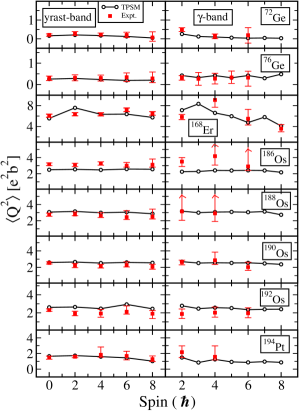
Figure 11: (Color online) Centroid $\langle Q^{2}\rangle$ of the yrast- and $\gamma$-bands for ^72,76Ge, ¹⁶⁸Er,^{186,188,190,192}Os and ¹⁹⁴Pt isotopes. Expt. data is taken from the Refs. [6, 9, 5, 7].

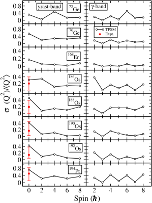
Figure 12: (Color online) Dispersion in $Q^{2}$ of the yrast- and $\gamma$-bands for ^72,76Ge, ¹⁶⁸Er,^{186,188,190,192}Os and ¹⁹⁴Pt isotopes.Expt. data is taken from the Refs. [6, 9, 5, 7].

Table LABEL:E2INBS1 provides the in-band stretched transition $E2(I\rightarrow\\ (I-2))$ matrix elements for the $\gamma\gamma$-bands. There is no data available for any of the nuclides. For the excited $0_{2}^{+}$-bands only one transition in ⁷²Ge is available. The measured experimental value indicates a deformation that is reduced by a factor of 0.73 as compared to the deformation used in the TPSM calculations.

The $I\rightarrow(I-1)$ in-band transitions are listed in Table LABEL:E2INBS2 for the $\gamma$- and $\gamma\gamma$-bands. Evidently, TPSM values are in good agreement with the measured ones. There are no measured intra-band matrix elements for the $\gamma\gamma$-bands to compare with the TPSM values.

Table LABEL:E2INTERBS1 provides the $I\rightarrow(I-2)$ inter-band $E2$ matrix elements for the transitions $\gamma\gamma\rightarrow$ yrast, $\gamma\gamma\rightarrow\gamma$, $0_{2}^{+}\rightarrow$ yrast, $0_{2}^{+}\rightarrow\gamma$ and excited $0^{+}\rightarrow\gamma\gamma$. The $\gamma\rightarrow$ yrast matrix elements are measured for all the eight nuclei studied, at least, up to $I=6$. The TPSM values agree within the error bars with the corresponding measured values.

The $I\rightarrow(I-1)$ inter-band transitions matrix elements are listed in Table LABEL:E2INTERBS2. Only the matrix elements between the $\gamma$- and yrast-bands in ⁷⁶Ge and the matrix elements between the $\gamma$- and $\gamma\gamma$-bands in the Osmium isotopes are measured, which deviate from the TPSM values. The discrepancy for ¹⁸⁶Os has already been attributed to the two-quasiparticle nature of the $4^{+}_{3}$ TPSM state in contrast to its $\gamma\gamma$ nature in experimental data.

Table LABEL:E2INTERBS30 provides the $I\rightarrow(I+1)$ inter band matrix elements. The TPSM reasonably accounts for the measured $\gamma\rightarrow$ yrast values. There are no experimental matrix elements available for the other transitions. More data are required to better analyze the TPSM predictions.

Table LABEL:E2INTERBS3 quotes the $I\rightarrow(I+2)$ inter-band matrix elements and between the yrast- and $\gamma$-band, which are reasonably well reproduced. The TPSM matrix elements from the $\gamma\gamma$ to the yrast-band and to the $\gamma$-band show significant deviations from the few observed values. As already mentioned, the reason for these deviations might be attributed to the incorrect description of the fragmentation of the collective $\gamma\gamma$-excitation. The matrix element for transitions between the $0^{+}_{2}$-band, and the $\gamma$- and yrast-bands are provided in the tables as well.

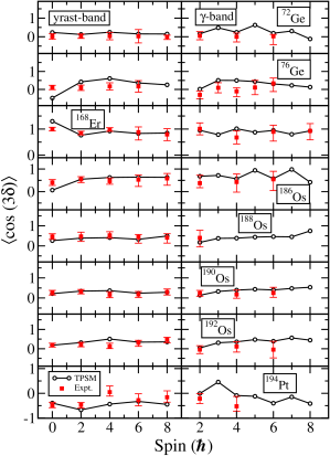
Figure 13: (Color online) Centroid $\langle\textrm{cos}3\delta\rangle$ of the yrast- and $\gamma$-bands for ^72,76Ge, ¹⁶⁸Er, ^{186,188,190,192}Os and ¹⁹⁴Pt isotopes. Expt. data is taken from the Refs. [6, 9, 5, 7].

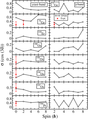
Figure 14: (Color online) Dispersion in $\textrm{cos}3\delta$ of the yrast- and $\gamma$-bands for ^72,76Ge, ¹⁶⁸Er,^{186,188,190,192}Os and ¹⁹⁴Pt isotopes. Expt. data is taken from the Refs. [6, 9, 5, 7].

IV.3 Quadrupole shape invariants

The quadrupole shape invariants have been evaluated using the coupled channel least-squares search code, GOSIA [2]. These quantities provide model-independent information about the shape of the system and are evaluated using the $E2$ matrix elements deduced from Coulomb excitation experiments [1, 7, 5, 6, 9, 10]. The shape-invariants analysis is possible for all the eight nuclei studied in the present work as large sets of $E2$ matrix elements have been obtained using COULEX experiments. As a matter of fact, the availability of the large set of data for these isotopes is the reason that we decided to perform a detailed analysis for these nuclides.

In principle, the evaluation of a shape invariant requires all the $E2$ matrix elements involved in the multiple sums, the number of which becomes quite large. In practice, on the experimental side one is forced to truncate the sums to the matrix elements that are measured in the COULEX experiments. We have carried out the GOSIA analysis including all TPSM evaluated matrix elements within and between yrast-, $\gamma$-, $\gamma\gamma$- and $0^{+}_{2}$-bands up to $I=10$, which are 187 in number and listed in Tables LABEL:E2INBD-LABEL:E2INTERBS3. In order to investigate possible truncation errors, we carried out another set of calculations with only those TPSM matrix elements for which the experimental $E2$ values have been deduced from the COULEX data. In most cases the results were close enough to justify the comparison of the experimental shape invariants with the TPSM derived quantities from the full set. There are exceptions where the two differ and will be commented in the following.

In our previous publication [20], we performed the shape-invariants analysis for ¹⁰⁴Ru. It was shown that TPSM calculated centroids and fluctuations of the quadrupole degree of freedom were in good agreement with those derived from the measured $E2$ matrix elements. The analysis indicated that this nucleus is $\gamma$-soft, which was quite unexpected because TPSM approach employs a fixed $\gamma$ value for the mean-field potential. One would have expected that the resultant shape invariants to lead to a $\gamma$-rigid shape. However, it was demonstrated that mixing of multi-quasiparticle excitations transforms the character of the system from $\gamma$-rigid to $\gamma$-soft. It is shown that for a few nuclei studied in the present work, the shape also transforms from $\gamma$-rigid and $\gamma$-soft in conformity with the shape inferred from the COULEX data.

Figs. 11 to 14 compare the shape invariants calculated from the TPSM $E2$ matrix elements with those evaluated from the experimental matrix elements, which were discussed in the previous section. Fig. 11 displays for the yrast- and the $\gamma$-bands the quantity $\langle Q^{2}\rangle$, which is a measure of the deviation from the spherical shape. It is approximately proportional to the mean value, $\langle\beta^{2}\rangle$, of the deformation parameter of the collective model [20]. This quantity is almost constant for the yrast- and $\gamma$-bands of all the eight nuclei studied, except for the $\gamma$-band in ¹⁶⁸Er, which will be discussed below. The dispersions $\sigma(Q^{2})/\langle Q^{2}\rangle$ in Fig. 12 are small for the yrast-bands, except for the Germanium isotopes. For the $\gamma$-bands, $\sigma(Q^{2})/\langle Q^{2}\rangle$ shows a larger even-odd staggering as compared to the weaker staggering in the yrast-bands. This staggering is analogous to those found for $S(I)$ of the energies, the origin of which has been discussed in Ref. [24].

Fig. 13 displays the centroids $\langle\cos(3\delta)\rangle$, which approximately represent the mean values of $\cos 3\gamma$ of the triaxiality parameter. The detailed relation is discussed in our previous publication [20]. It is evident from the figure that, in general, the agreement between the calculated and the experimental values is quite reasonable.

Fig. 14 depicts the dispersion, $\sigma(\cos(3\delta))$. The experimental values are available only for a few cases [1, 7, 9]. The TPSM values are in good agreement, except for ⁷⁶Ge. The TPSM calculations with the restricted set of $E2$ matrix elements as used to obtain the experimental dispersion gave a smaller value, which falls into the range of the error bars. Hence, we attribute the discrepancy to the restriction of the experimental $E2$ matrix elements available from the COULEX experiments. It is expected that the errors caused by the restricted set, increase with the power of the involved tensor products, which is highest for $\sigma(\cos(3\delta))$. In the $\gamma$-bands of several nuclei, $\sigma(\cos(3\delta))$ shows an even-odd effect with no clear phase relation to the energy staggering $S(I)$.

We shall now discuss the TPSM results of the individual systems and compare them with earlier investigations. The nucleus ⁷²Ge is one among only three nuclides in the periodic table far from closed shell that has $0^{+}_{2}$ as the first excited state. Its experimental energy staggering $S(I)$ in Fig. 4 displays the even-$I$-down pattern that corresponds to the $\gamma$-soft shape in the context of the collective model. Detailed investigation of this nucleus has been performed using COULEX data with a total of 46 $E2$ and $M1$ matrix elements extracted [6], which were then used to obtain the quadrupole shape invariants. First of all, the TPSM calculation reproduces the even-$I$-down pattern of $S(I)$, though with a smaller amplitude. For the yrast- and $\gamma$-bands, the empirical $\langle Q^{2}\rangle$ indicates a constant deformation and $\langle\textrm{cos}(3\delta)\rangle$ implies a constant triaxiality of $\gamma\approx 30^{\circ}$ and the TPSM results are in good agreement. For the $\gamma$-band, $\langle\textrm{cos}3\delta\rangle$ displays an even-$I$-down staggering in conformity with the energy staggering $S(I)$. The dispersions $\sigma(\textrm{cos}(3\delta))$ indicate large fluctuations for the ground state, which decrease with $I$ in the yrast-band. For the $\gamma$-band, the fluctuations are small except for $I=2$.

The experimental shape invariants of Ref. [6] indicate that the yrast- and the excited $0^{+}_{2}$-bands have similar deformation and triaxiality parameters, and the authors suggested that the two bands represent an equal mixing of two different unperturbed triaxiality deformed shapes. The present TPSM calculation is unable to reproduce the very low experimental energy of $0^{+}_{2}$ state, which might be a pairing vibration. The calculated large dispersion, $\sigma(Q^{2})/\langle Q^{2}\rangle$, of the $0^{+}_{1}$ state may be an indirect evidence for the existence of such a low-lying $0^{+}_{2}$ state.

The energy staggering $S(I)$ of the $\gamma$-band in ⁷⁶Ge shows the even-$I$-up pattern which in the context of the collective model classifies the nucleus as being one of the rare examples of being "$\gamma$-rigid" [23]. However, as discussed in Ref. [24], the amplitude of $S(I)$ is far below the Davydov-Filippov limit of a rigid triaxial rotor. For this reason the authors of Ref. [9] have extensively studied this nucleus by means of COULEX data in order to probe directly its triaxiality. The measured $\gamma$-ray intensities were analyzed using the computer code GOSIA, and absolute values and signs of 103 matrix elements were determined.

For the yrast- and $\gamma$-bands, $\langle Q^{2}\rangle$ in Fig. 11 indicates a constant value of deformation. The experimental $\langle\textrm{cos}(3\delta)\rangle$ values for the two bands indicate triaxiality close to the maximum of $30^{\circ}$. The TPSM calculations suggest a gradual transition from a slightly oblate to a slightly prolate shape for the yrast-band. The TPSM calculations with the reduced set of matrix elements gives a more constant value, which is closer to the value derived from the experimental $E2$ matrix elements. For the $\gamma$-band, the TPSM calculations give a smooth $I$-dependence with values that are skewed towards the prolate side.

Both for ^72,76Ge isotopes, the TPSM calculations with the restricted set of $E2$ matrix elements give smaller values of $\sigma(\textrm{cos}(3\delta))$ than calculation with the full set for the $I=$ 0 and 2 yrast states. As mentioned already, the TPSM values from the restricted set agree well with the experimental values in ⁷⁶Ge. Therefore, the small fluctuations of $\gamma$ around its mean values, indicated by the experimental values, may be an artifact, and the actual fluctuations are substantially larger.

The TPSM values for $I=$0, 2 and 4 of $\langle\textrm{cos}(3\delta)\rangle$ and $\sigma(\textrm{cos}(3\delta))$ do not differ much between ⁷²Ge and ⁷⁶Ge, indicating for both nuclei substantial triaxiality and softness, which decreases with $I$. Thus, the difference between the respective even-$I$-down and even-$I$-up pattern of the staggering of the $\gamma$-band energies is not reflected by the $E2$ transition probabilities. It is caused by the difference of the energy and structure of the $0^{+}_{2}$ state, the origin of which remains to be ascertained.

The Erbium isotopes are examples of well deformed prolate nuclei. These nuclides confirm many predictions of the quadrupole collective model of Bohr and Mottelson [4], which have been tested extensively in the past. In particular, ¹⁶⁸Er is one of the best studied nuclides using different experimental techniques [57] and more than 36 rotational bands have been populated for this system. A comprehensive analysis of the band structure is given in Ref. [58].

As expected for a well deformed prolate nuclei, $\langle Q^{2}\rangle$ is approximately constant for the yrast-band. For the $\gamma$-band, TPSM values are about the same as the experimental values, except for a slight bump at $I=3$, which we could not relate to irregularities in the individual matrix elements of ¹⁶⁸Er in Figs. 11 to 14. The dispersion $\sigma(Q^{2})/\langle Q^{2}\rangle$ of the yrast-band decreases with $I$, indicating a stabilization of the deformation. This same observation holds for the $\gamma$-band.

The mean values $\langle\cos(3\delta)\rangle$ are 0.8-0.9 for the yrast- and $\gamma$-bands of ¹⁶⁸Er, which correspond to root mean square values of $\sqrt{\langle\gamma^{2}\rangle}=8^{\circ}-12^{\circ}$. From the perspective of the collective model, one would expect larger fluctuations in the $\gamma$-band than in the yrast-band, because the quantum fluctuations of the one-phonon state are larger than the fluctuations of the ground state. However, this is not the case in the microscopic TPSM calculations, where the TPSM results are consistent with the experimental data for ¹⁶⁸Er, within the error bars.

According to the collective model, the $0^{+}_{2}$ state should be the collective $\beta$ vibration with an enhanced $E2$ transition to the $2^{+}_{1}$ state of the yrast-band. The experimental limit for the absolute value of the matrix element $\langle 0^{+}_{2}||E2||2^{+}_{1}\rangle$ which is below 0.2 eb [5] is close to the TPSM value of 0.456 eb (see Table LABEL:E2INTERBS3) and indicates the non-collective nature of the transitions from the excited $0^{+}_{2}$ state ($\langle 0^{+}_{2}||E2||2^{+}_{1}\rangle/\langle 0^{+}_{1}||E2||2^{+}_{1}\rangle=0.09$). The other TPSM inter-band transition matrix elements that connect $0^{+}_{2}$-band with the $\gamma$- and yrast-bands are also of the single particle order (see Tables LABEL:E2INTERBS1-LABEL:E2INTERBS3).

The even-even Osmium and Platinum isotopes are expected to exhibit a transition from prolate to oblate shape through triaxial intermediate shapes with increasing $N$ [59, 60]. In a detailed COULEX experiment, ¹⁸⁶Os, ¹⁸⁸Os, ¹⁹⁰Os, ¹⁹²Os and ¹⁹⁴Pt have been studied, and large sets of $E2$ matrix elements have been deduced [7] for each of these nuclides.

The values $\langle Q^{2}\rangle\approx 3(\mathrm{eb})^{2}$ in Fig. 11 indicate an $I$-independent deformation for the yrast- and $\gamma$-bands for the Os- and Pt-nuclides, which reflects a moderate collectivity of $B(E2,I\rightarrow I-2)=40-90$ Wu of the intra-band transitions. The TPSM calculations reproduce the experimental values reasonably well, only the ¹⁸⁶Os values are slightly underestimated (see Fig. 5). The dispersions $\sigma(Q^{2})/\langle Q^{2}\rangle$ show that the fluctuations of the deformation around the mean values are small except for the ground state. The experimental values known for the ground state have large error bars and it is difficult to make an assessment of the predicted values. We would like to add that calculations with the restricted TPSM set, the dispersions for the ground states are much smaller, which is a general observation other nuclides as well.

The values of the centroid of $\langle\textrm{cos}3\delta\rangle$ of the yrast-band show a gradual shape development with $N$ : $\delta\approx 20^{\circ}$ for ¹⁸⁶Os and $\delta\approx-20^{\circ}$ for ¹⁹⁴Pt. The values of the $\gamma$-band develop with $N$ in a similar manner. It is noted from Fig. 13 that experimental values of $\langle\textrm{cos}3\delta\rangle$ are reproduced quite well by the TPSM calculations. The experimental values for dispersion are available for the $0^{+}_{1}$ ground state for ^188,190,192 and ¹⁹⁴Pt and the TPSM values are noted to be in agreement.

Based on the phase of the TPSM energy staggering $S(I)$ in Fig. 4, the nuclides ^{186,188,190,192}Os and ¹⁹⁴Pt are classified as "$\gamma$-soft, rigid, soft, rigid, rigid", respectively. However, the TPSM dispersions $\sigma(\textrm{cos}(3\delta)$, which provide direct insight into the softness of the $\gamma$ degree of freedom, do not correlate with this pattern. The experimental data also shows this disparity. This inference demonstrates that the correlation between the phase of the staggering parameter $S(I)$ and the softness of the $\gamma$ mode, which emerges in the eigenstates of the collective Bohr Hamiltonian (see Ref. [24] and earlier work cited therein) is not realized in the microscopic TPSM approach for these nuclei.

V Summary and conclusions

In the present work, we have performed a systematic study of the $E2$ matrix elements of ⁷²Ge, ⁷⁶Ge, ¹⁶⁸Er, ¹⁸⁶Os, ¹⁸⁸Os, ¹⁹⁰Os, ¹⁹²Os and ¹⁹⁴Pt nuclides. For these eight nuclides, extensive multi-step Coulomb excitation experiments have been performed and large sets of $E2$ matrix elements have been deduced, which make it possible to directly ascertain the intrinsic shape of the nucleus by using the Kumar-Cline shape invariant sum rule analysis [1, 3]. In most of the cases, the $E2$ matrix elements have been analyzed using the phenomenological collective model of Bohr and Mottelson and also the microscopic versions of it [4, 5, 6, 7, 9, 10]. These models have been partially successful in correlating the experimental data for yrast- and $\gamma$-bands, and it has been possible to account for the overall behaviour of the measured properties at low spin. However, these models are clearly limited in scope as quasiparticle excitations are not included, and high-spin states cannot be investigated using these approaches. As COULEX data is now becoming available for the intermediate- and high-spin regions, it is imperative to include quasiparticle excitations in the model description.

Further, there has been a long-standing problem to describe the excited $0^{+}$ states observed in many nuclei using the collective models. These states are collective in nature in these models and transitions to the $\gamma$- or yrast-bands should be enhanced as compared to the Weisskopf estimate. However, the measured transitions are less than the single-particle estimate and, therefore, have non-collective character, in contradiction to the prediction of the Bohr-Mottelson collective model.

To elucidate the rich data on $E2$ matrix elements, we have employed the multi-quasiparticle TPSM approach and evaluated a large set of 187 matrix elements for each of the eight nuclei investigated in the present work. The advantage of the TPSM approach is that first of all it is microscopic in nature with the Hamiltonian consisting of pairing and quadrupole terms. Secondly, the model space includes multi-quasiparticle states. In the present investigation of even-even systems, two-neutron, two-proton and two-proton$+$two-neutron quasiparticle states have been considered apart from the zero-quasiparticle vacuum configuration. The angular-momentum projected states from these quasiparticle configurations are then employed to diagonalize the shell model Hamiltonian. In this way, the TPSM is a useful tool to include the correlations going beyond the mean-field.

The TPSM approach describes the appearance of a collective $\gamma$ mode by projecting states with different values of angular momentum projection quantum number, $K$, onto the 3-axis of triaxial shape from the considered quasiparticle configurations. The subsequent mixing of these basis states generates the collective excitations due to the $\gamma$ degree of freedom. The set of $K$=2, 4, 6, … states projected from the triaxial vacuum configuration generates the collective $\gamma$-, $\gamma\gamma$-,… band structures, which have the character of triaxial rotor states. The admixture of states with different $K$ projected from two- and four-quasiparticle configurations then account for the deviations from rigid rotation. The TPSM configuration space includes, $\gamma$-excitation from all the quasiparticle configurations [22]. The $\gamma$-bands built on two-quasiparticle bands have been identified [61].

The in-band and inter-band $E2$ transition matrix elements for the yrast-, $\gamma$-, $\gamma\gamma$-, $0^{+}_{2}$-bands have been investigated in detail and compared with the measured values, wherever available. The $E2$ matrix elements have been listed in Tables LABEL:E2INBD to LABEL:E2INTERBS3 of the appendix A up to $I=10$ because the data in most of the cases is only available below or up this spin. These are 187 matrix elements in number for each nucleus. However, we have evaluated the $E2$ transition matrix elements up to $I=20$, which can be made available to the interested researchers upon request.

It is evident from the comparisons provided in the figures and tables that TPSM provides a reasonable description of the measured transition matrix elements. A few discrepancies are noted in the inter-band matrix elements for high-spin states. Since these matrix elements are retarded, small admixtures from neglected configurations could cause significant changes. Further, the interaction employed in the TPSM analysis is quite simplistic and a more realistic is expected to improve the agreement with the data.

From the $E2$ matrix elements, we evaluated the Kumar-Cline quadrupole shape invariants $\langle Q^{2}\rangle$, $\langle\textrm{cos}(3\delta)\rangle$, which represent the mean value of the deformation and the triaxiality of the nuclear shape. In addition, we calculated the dispersions $\sigma(Q^{2})/\langle Q^{2}\rangle$ and $\sigma(\textrm{cos}(3\delta))$, which provide an estimate of the fluctuations around the respective mean values, i.e., of the $\beta$ and $\gamma$-softness of the shape.

From the detailed analysis of the excitation energies, $E2$ matrix elements and quadrupole shape invariants results, it is possible to draw the following inferences $:$

1. The TPSM results reproduce very well the energies of the yrast- and $\gamma$-bands. The model accounts in detail the rotational alignment of the high-j quasiparticles as demonstrated in the $\hbar\omega(I)$ plots. The even-odd staggering parameter $S(I)$ of the energies of the $\gamma$-band is accurately reproduced, in particular the change of its phase with $N$ in the Os-Pt isotopic chain. Based on the collective Bohr Hamiltonian, the even-$I$-down pattern of $S(J)$ has been associated with a shape that is soft in the $\gamma$ degree of freedom and the even-$I$-up pattern with a shape that is rigid [62, 63, 58]. The authors of Ref. [24, 20, 39] explained this correlation in terms of the repulsion between the even-$I$ states of the $\gamma$-band and the $\gamma\gamma$-band, which is low in $\gamma$-soft and high in $\gamma$-rigid nuclei. In the case of the TPSM, the staggering is caused by the repulsion between even-$I$ states of the $\gamma$-band and of several $0^{+}$-bands built on excited two-quasiparticle bands. The energy and structure of the lowest two-quasiparticle bands depend on $N$, which explains the rapid change of the phase of $S(I)$ with $N$ found in the TPSM calculations, in accordance with the experimental data.

2. Yrast- and $\gamma$-bands in the ⁷²Ge (even-$I$-down) and ⁷⁶Ge (even-$I$-up) are strongly triaxial on the average ($\langle\gamma\rangle\sim 30^{\circ}$) and in conformity with the experimental data. Based on the dispersions, $\sigma(\textrm{cos}(3\delta))$, the $I=$0, 2, 4 yrast states are found to be $\gamma$-soft in both nuclei. At higher $I$, the yrast states of ⁷²Ge are predicted to become $\gamma$-rigid and those of ⁷⁶Ge as $\gamma$-soft. For the $\gamma$-bands, the TPSM predicts moderate $\gamma$-softness in both the nuclei. The small experimental $\gamma$-dispersion values of ⁷⁶Ge indicate rigidity. However, this could be an artifact of the restricted number of matrix elements extracted from the COULEX experiment. As a matter of fact, we have also evaluated centriods and dispersions with the same restricted set of TPSM $E2$ matrix elements as used in the data, and obtained smaller dispersions as in the experimental work.

   It is important to point out that the comparable softness of the two isotopes derived from the $E2$ matrix elements is at variance with the staggering pattern of the $\gamma$-bands, which is reproduced by the TPSM as well. In the context of the collective model, the even-$I$-down pattern in ⁷²Ge suggest $\gamma$-softness while the even-$I$-up pattern in ⁷⁶Ge suggest $\gamma$-rigidity. The difference illustrates the limitations of a purely collective model as compared with a microscopic approach.

3. For the yrast- and $\gamma$-bands in the Osmium isotopes, the average triaxiality increases from $\langle\gamma\rangle\sim 20^{\circ}$ in ¹⁸⁶Os to $\langle\gamma\rangle\sim 25^{\circ}$ in ¹⁹²Os, with the TPSM values agreeing well with the experimental quantities. The dispersions, $\sigma(\textrm{cos}(3\delta))$ suggest a gradual increase of $\gamma$-softness along the considered isotopic chain, which is seen in the experimental data as well. This is at variance with the macroscopic collective model [12, 11], according to which the phase of the staggering parameter associated with ^{186,188,190,192}Os has the characteristics of being $\gamma$-soft, -rigid, -soft, -rigid, respectively. The corresponding staggering pattern is reproduced by the TPSM calculations, while the moderate $\gamma$-softness derived for all isotopes from the $E2$ matrix elements is consistent with the COULEX data.

4. The TPSM predicts an average triaxiality of $\langle\gamma\rangle\sim 40^{\circ}$ in the yrast-band and $\langle\gamma\rangle\sim 30^{\circ}$ in the $\gamma$-band for ¹⁹⁴Pt, which agrees with the experimental data. The TPSM dispersions indicate large fluctuations in $\gamma$, while the energy staggering $S(I)$ shows the even-$I$-up pattern.

5. ¹⁶⁸Er is shown to be a prolate system with small fluctuations in $\gamma$.

6. The excited $0^{+}_{2}$-bands of the studied nuclei, which in the framework of the collective Bohr Hamiltonian appear as a mixture of $\gamma\gamma$ and $\beta$ vibrational excitations, have been shown to be based on two-quasiparticle states. Accordingly, the transition matrix elements to the yrast-bands and $\gamma$-bands are of single particle order in magnitude. Similarly, the structures with the band head of $I=4$ cannot be considered as collective $\gamma\gamma$ structures. These are predominantly two-quasiparticle states. In both cases, the TPSM values do not correlate well with the experimental values of these retarded transitions. The present version of the TPSM approach seems to be unable to describe quantitatively the fragmentation of the collective $\gamma\gamma$-excitations among the two-quasiparticle states.

7. For the studied nuclei, TPSM results do not reveal the correlation between the phase of $S(I)$ and the shape fluctuations derived from the $E2$ matrix elements that exists for the collective Bohr Hamiltonian (even-$I$-down - $\gamma$-soft; even-$I$-up - $\gamma$-rigid). The experimental dispersions, $\sigma(\textrm{cos}(3\delta))$ are only known for the ground states of ⁷⁶Ge, ^{186,188,190,192}Os and ¹⁹⁴Pt, which are too uncertain to confirm the TPSM findings.

8. The analysis of the individual $E2$ transition matrix elements and of the derived quadrupole shape invariant quantities reveals that although the TPSM approach generates multi-quasiparticle basis from the Nilsson potential with a fixed triaxiality parameter $\gamma$, the subsequent configuration mixing accounts for the transitional shape features from $\gamma$-rigid to that of $\gamma$-soft. Our study adds eight examples to the case of ¹⁰⁴Ru, where we demonstrated this capability of the TPSM approach for the first time [20].

We realized, after the completion of the present work, that COULEX data is also available for other nuclides which include ^76,80,82Se, ¹⁰⁰Mo and ¹¹⁰Pd [64, 65, 1, 66]. These nuclides also have sufficient sets of $E2$ matrix elements that can be used to perform the shape invariant analysis. The TPSM results on $E2$ matrix elements and shape invariants for these nuclides will be presented in a forthcoming publication.

VI ACKNOWLEDGEMENTS

One of the authors (NN) would like to acknowledge Department of Science and Technology (Govt. of India) for the award of INSPIRE fellowship under sanction No. DST/INSPIRE Fellowship/[IF200508].

Appendix A Tables of the E2 matrix elements

Table A1: Reduced TPSM E2 diagonal matrix elements in ^72,76Ge, ¹⁶⁸Er,^{186,188,190,192}Os and ¹⁹⁴Pt. Available experimental matrix elements are listed in parenthesis below the TPSM values, where the errors are quoted in square brackets.

$I_{i}\rightarrow I_{f}$	72Ge	76Ge	168Er	186Os	188Os	190Os	192Os	194Pt
$I_{yrast}\rightarrow I_{yrast}$
$2_{1}\rightarrow 2_{1}$	-0.156	-0.237	-3.97	-1.6	-1.861	-1.698	-1.609	0.683
	(-0.16 [${}^{+0.07}_{-0.02}$])	(-0.24 [2])	(-3.25[${}_{-0.25}^{+0.10}$ ])	(-1.75 [${}^{+22}_{-13}$])	(-1.73 [${}^{+19}_{-5}$])	(-1.25 [${}^{+22}_{-13}$])	(-1.21 [${}^{+6}_{-17}$])	(0.54 [${}^{+8}_{-6}$])
$4_{1}\rightarrow 4_{1}$	-0.159	-0.238	-3.76	-1.965	-2.211	-1.974	-1.672	0.514
	(-0.14 [${}^{+0.09}_{-0.04}$])	(-0.26 [${}^{+0.01}_{-0.07}$])	(-3.13[${}_{-0.09}^{+0.42}$])	(-2.02 [${}^{+39}_{-18}$])	(-2.00 [${}^{+9}_{-20}$])	(-1.28 [${}^{+27}_{-19}$])	(-0.73 [${}^{+26}_{-6}$])	(1.00 [${}^{+12}_{-14}$])
$6_{1}\rightarrow 6_{1}$	-0.171	-0.209	-4.77	-2.191	-2.339	-1.969	-1.597	0.121
	(0.20 [${}^{+0.08}_{-0.25}$])	(-0.23 [${}^{+0.09}_{-0.04}$])	(-5.25[${}_{-0.17}^{+0.16}$ ])	(-1.67 [${}^{+29}_{-31}$])	(-1.60 [${}^{+18}_{-33}$])	(-0.91 [${}^{+24}_{-15}$])	(-1.16 [${}^{+11}_{-26}$])	(0.28 [${}^{+12}_{-27}$])
$8_{1}\rightarrow 8_{1}$	-0.416	-0.198	-4.98	-2.299	-2.296	-1.788	-1.573	0.389
			(-6.63[${}_{-0.27}^{+0.20}$ ])	(-2.26 [${}^{+24}_{-108}$])	(-1.38 [${}^{+44}_{-26}$])	(-0.94 [${}^{+49}_{-41}$])	(-1.31 [${}^{+18}_{-36}$])	([-0.10, 0.43])
$10_{1}\rightarrow 10_{1}$	-0.114	0.188	-4.86	-2.215	-2.161	-1.588	-1.616	0.9
			(-5.60[${}_{-0.20}^{+0.20}$ ])	([-4.2, -1.3])	([-1.7, -0.8])	([-1.9, -0.7])	([-2.5, 1.0])
$I_{\gamma}\rightarrow I_{\gamma}$
$2_{2}\rightarrow 2_{2}$	0.056	0.24	2.97	1.588	1.859	1.697	1.612	-0.566
	(0.179 [${}^{+0.03}_{-0.06}$])	(0.26 [${}^{+0.02}_{-0.05}$])	(2.85[${}_{-0.09}^{+0.09}$])	(2.12 [${}^{+6}_{-22}$])	(2.10 [${}^{+9}_{-6}$])	(1.53 [${}^{+6}_{-31}$])	(0.985 [${}^{+45}_{-85}$])	(-0.40 [${}^{+12}_{-5}$])
$3_{1}\rightarrow 3_{1}$	0.005	0.102	2.01	0.004	0.012	0.013	0.006	-0.051
	(0.001 $\pm$0.521)	(0.13 [${}^{+0.08}_{-0.10}$])
$4_{2}\rightarrow 4_{2}$	-0.258	-0.222	-1.65	-0.958	-1.149	-1.115	-1.342	-0.014
	(-0.29 [${}^{+0.04}_{-0.20}$])	(-0.24 [${}^{+0.08}_{-0.04}$])	(-1.86[${}_{-0.16}^{+0.10}$])	(-1.12 [${}^{+25}_{-23}$])	(-1.22 [${}^{+16}_{-10}$])	(-1.29 [${}^{+20}_{-25}$])	(-0.83 [${}^{+9}_{-8}$])	(-0.07 [14])
$5_{1}\rightarrow 5_{1}$	-0.174	-0.209	-2.25	-1.332	-1.513	-1.403	-1.296	0.445
$6_{2}\rightarrow 6_{2}$	-0.275	-0.324	-2.54	-2.011	-2.441	-2.435	-2.636	0.06
		(1.3 [${}^{+0.2}_{-0.2}$])	(-2.04[${}_{-0.25}^{+0.13}$])	([-0.9, 0.6])	(-1.33 [${}^{+23}_{-56}$])	(-0.80 [${}^{+47}_{-27}$])	(-1.35 [${}^{+11}_{-37}$])	(0.41 [${}^{+26}_{-22}$])
$7_{1}\rightarrow 7_{1}$	-0.262	-0.245	-2.91	-1.964	-2.209	-2.044	-1.889	0.226
$8_{2}\rightarrow 8_{2}$	-0.227	-0.485	-2.72	-2.587	-3.309	-3.343	-3.264	0.56
			(-2.42[${}_{-0.14}^{+0.80}$])		([-2.4, -0.8])	(-1.05 [${}^{+62}_{-38}$])	(-0.91 [${}^{+49}_{-34}$])
$9_{1}\rightarrow 9_{1}$	-0.351	-0.143	-2.18	-2.312	-2.59	-2.362	-2.329	0.35
$10_{2}\rightarrow 10_{2}$	-0.157	-0.477	-2.47	-1.886	-3.895	-3.889	-2.688	-0.046
			(-1.2[${}_{-1.4}^{+3.5}$])
$I_{\gamma\gamma}\rightarrow I_{\gamma\gamma}$
$4_{3}\rightarrow 4_{3}$	0.319	0.783	1.36	-1.958	0.379	3.096	3.026	0.229
				(2.35 [${}^{+92}_{-69}$])	(2.68 [${}^{+22}_{-19}$])	(1.02 [${}^{+18}_{-4}$])	(1.28 [${}^{+15}_{-41}$])
$5_{2}\rightarrow 5_{2}$	0.145	0.36	-0.37	1.289	1.52	1.388	1.28	0.258
$6_{3}\rightarrow 6_{3}$	-0.367	-0.091	-1.39	-2.44	-0.897	-2.414	-2.785	0.355
$7_{2}\rightarrow 7_{2}$	-0.252	-0.161	-2.01	-1.921	-0.543	-0.501	-1.344	0.093
$8_{3}\rightarrow 8_{3}$	-0.109	-0.569	-2.42	-2.315	-2.93	-2.872	-2.411	0.165
$9_{2}\rightarrow 9_{2}$	-0.187	-0.396	-2.71	-2.249	-1.616	-2.659	-1.988	1.192
$10_{3}\rightarrow 10_{3}$	-0.406	-0.945	-2.89	-2.405	-0.982	2.62	-2.022	0.864
$I_{0_{2}^{+}}\rightarrow I_{0_{2}^{+}}$
$2_{3}\rightarrow 2_{3}$	0.167	0.295	-2.191	-1.233	-1.438	-1.142	-1.212	0.622
	(-0.02 [${}^{+0.03}_{-0.14}$])
$4_{4}\rightarrow 4_{4}$	0.135	0.226	-2.071	-1.163	-1.316	-1.026	-1.007	-0.149
$6_{4}\rightarrow 6_{4}$	-0.145	-0.033	-2.021	-1.111	-1.147	-1.047	-0.844	-0.117
$8_{4}\rightarrow 8_{4}$	-0.169	-0.308	-1.973	-0.969	-0.954	-0.91	-1.094	0.911
$10_{4}\rightarrow 10_{4}$	0.036	-0.194	-1.919	-0.802	-1.235	-0.759	-0.634	0.447

Table A2: Reduced TPSM E2 inter-band matrix elements for $I\rightarrow I$ transitions in ^72,76Ge, ^{186,188,190,192}Os and ¹⁹⁴Pt. Available experimental matrix elements are listed in parenthesis below the TPSM values, where the errors are quoted in square brackets. The sign convention of the COULEX experiments is used, where the sign of the numerical TPSM calculation is quoted in parentheses if changed.

$I_{i}\rightarrow I_{f}$	72Ge	76Ge	168Er	186Os	188Os	190Os	192Os	194Pt
$I_{\gamma}\rightarrow I_{Yrast}$
$2_{2}\rightarrow 2_{1}$	0.479	0.667	0.41	0.999	0.951	0.909	1.064	1.351
	(0.65 [${}^{+0.01}_{-0.02}$])	(0.535 [${}^{+0.03}_{-0.07}$])	(0.47[${}_{-0.01}^{+0.02}$ ])	(0.897 [${}^{+64}_{-14}$])	(0.865 [11])	(1.065 [${}^{+20}_{-37}$])	(1.23 [${}^{+34}_{-16}$])	(1.517 [${}^{+11}_{-18}$])
$4_{2}\rightarrow 4_{1}$	0.309	0.613	0.64	1.42	1.395	1.344	1.432	1.644
	(0.43 [10])	(0.61 [1])	(0.72[${}_{-0.02}^{+0.02}$ ])	(1.22 [${}^{+62}_{-55}$])	(1.1 [3])	(1.435 [${}^{+43}_{-45}$])	(1.35 [${}^{+8}_{-4}$])	(1.51 [${}^{+6}_{-5}$])
$6_{2}\rightarrow 6_{1}$	0.022	0.621	0.65	1.686	1.633	1.541	1.486	1.029
	(0.18 [${}^{0.25}_{-0.08}$])	(1.2 [${}^{+0.2}_{-0.1}$])	(0.74[${}_{-0.02}^{+0.04}$ ])	(1.37 [${}^{+9}_{-11}$])	(1.46 [${}^{+13}_{-25}$])	(1.76 [${}^{+20}_{-15}$])	(1.49 [${}^{+15}_{-6}$])	(1.14 [${}^{+11}_{-24}$])
$8_{2}\rightarrow 8_{1}$	0.25	0.609	0.73	1.374 (-)	1.022	1.521	1.335	1.001
			(0.81[${}_{-0.05}^{+0.03}$ ])
$10_{2}\rightarrow 10_{1}$	0.004	0.633	0.81	0.029 (-)	1.673	1.372 (-)	1.077	1.139
$I_{\gamma\gamma}\rightarrow I_{Yrast}$
$4_{3}\rightarrow 4_{1}$	0.046	0.099	0.555	-0.006	0.019	0.028	0.074	0.001
						([-0.2, 0.2] )
$6_{3}\rightarrow 6_{1}$	0.267	0.114	0.683	-0.033	0.037	0.002	-0.283	-0.081
$8_{3}\rightarrow 8_{1}$	-0.038	-0.109	-0.794	-1.262	-0.022	-0.074	-0.205	0.034
$10_{3}\rightarrow 10_{1}$	0.173	-0.101	-0.9	-0.213	-0.092	-0.094	0.231	0.023
$I_{\gamma\gamma}\rightarrow I_{\gamma}$
$4_{3}\rightarrow 4_{2}$	0.359	0.597	0.015	-0.067	0.639	0.551	0.745	0.264
				(1.83 [${}^{+32}_{-34}$])	(1.64 [7])	(1.59 [${}^{+11}_{-17}$])	(1.19 [${}^{+8}_{-11}$])
$5_{2}\rightarrow 5_{1}$	0.188	0.496	-0.038	-0.907	0.896	-0.786	0.982	0.144
$6_{3}\rightarrow 6_{2}$	0.033	0.682	0.041	-0.072	-0.808	0.123	-0.126	0.162
$7_{2}\rightarrow 7_{1}$	0.029	-0.606	-0.085	0.333	-1.193	-0.073	-0.789	0.142
$8_{3}\rightarrow 8_{2}$	-0.007	-0.828	0.082	-0.199	-0.006	0.071	0.206	-0.329
$9_{2}\rightarrow 9_{1}$	0.038	-0.674	-0.154	0.117	-1.312	-0.074	0.593	0.203
$10_{3}\rightarrow 10_{2}$	-0.087	-0.921	0.138	0.087	0.026	0.124	-0.297	0.194
$I_{0_{2}^{+}}\rightarrow I_{Yrast}$
$2_{3}\rightarrow 2_{1}$	-0.047	-0.016	0.016	-0.024	-0.039	-0.024	0.002	0.013
	(0.243 [${}^{+0.002}_{-0.004}$])	(-0.126 [${}^{+0.006}_{-0.004}$])	($<|0.5|$)
$4_{4}\rightarrow 4_{1}$	0.103	-0.01	0.008	0.003	-0.016	0.009	-0.049	0.019
$6_{4}\rightarrow 6_{1}$	0.066	-0.131	0.006	0.346	0.028	-0.013	-0.047	-0.147
$8_{4}\rightarrow 8_{1}$	-0.028	0.039	0.003	0.003	0.016	-0.03	-0.216	0.165
$10_{4}\rightarrow 10_{1}$	-0.001	0.055	0.001	-0.687	0.015	0.05	-0.48	0.009
$I_{0_{2}^{+}}\rightarrow I_{\gamma}$
$2_{3}\rightarrow 2_{2}$	0.034	0.029	-0.013	0.014	0.003	0.017	0.103	0.153
	(0.49 [${}^{+0.02}_{-0.01}$])
$4_{4}\rightarrow 4_{2}$	0.186	0.162	-0.005	0.032	0.166	0.007	-0.131	-0.398
$6_{4}\rightarrow 6_{2}$	0.021	-0.21	-0.004	0.05	0.529	0.014	0.004	0.454
$8_{4}\rightarrow 8_{2}$	-0.123	-0.113	-0.002	-0.029	0.334	0.266	-0.178	-0.029
$10_{4}\rightarrow 10_{2}$	-0.071	0.138	0.001	-0.011	-0.146	-0.581	-0.169	-0.02
$I_{\gamma\gamma}\rightarrow I_{0_{2}^{+}}$
$4_{3}\rightarrow 4_{4}$	0.021	0.084	-0.005	0.016	0.006	0.105	0.323	0.214
$6_{3}\rightarrow 6_{4}$	0.008	-0.152	-0.003	-0.059	-0.013	0.303	0.04	0.32
$8_{3}\rightarrow 8_{4}$	0.262	-0.009	-0.001	0.035	0.325	0.557	-0.128	0.189
$10_{3}\rightarrow 10_{4}$	-0.063	0.011	0.001	0.031	-0.624	0.012	0.348	0.009

Table A3: Reduced TPSM E2 in-band matrix elements for transitions $I_{i}\rightarrow(I-2)_{f}$ in ^72,76Ge, ¹⁶⁸Er,^{186,188,190,192}Os and ¹⁹⁴Pt. Available experimental matrix elements are listed in parenthesis below the TPSM values, where the errors are quoted in square brackets. The sign convention of the COULEX experiments is used, where the sign of the numerical TPSM calculation is quoted in parentheses if changed.

$I_{i}\rightarrow I_{f}$	72Ge	76Ge	168Er	186Os	188Os	190Os	192Os	194Pt
$I_{yrast}\rightarrow(I-2)_{yrast}$
$2_{1}\rightarrow 0_{1}$	0.402	0.463	2.33	1.406	1.6	1.469	1.491	1.283
	(0.457 [4])	(0.526 [2])	(2.43[$\pm$0.07])	(1.674 [${}^{+25}_{-21}$])	(1.585 (10))	(1.53 [${}^{+20}_{-11}$])	(1.456 [${}^{+8}_{-9}$])	(1.208 [${}^{+49}_{-17}$])
$4_{1}\rightarrow 2_{1}$	0.768	0.72	3.99	2.304	2.621	2.407	2.458	1.921
	(0.90 [2])	(0.795 [5])	(3.92[$\pm$0.12])	(2.761 [${}^{+61}_{-70}$])	(2.642 (${}^{+25}_{-20}$))	(2.367 [${}^{+80}_{-31}$])	(2.115 [${}^{+29}_{-28}$])	(1.935 [${}^{+21}_{-13}$])
$6_{1}\rightarrow 4_{1}$	0.874	0.897	5.01	2.992	3.393	3.133	3.221	2.619
	(1.11 [${}^{+0.04}_{-0.05}$])	(1.11 [${}^{+0.03}_{-0.02}$])	(5.43[$\pm$0.16])	(3.89 [${}^{+8}_{-5}$])	(3.31 (4))	(2.97 [${}^{+63}_{-40}$])	(2.93 [${}^{+77}_{-44}$])	(2.9 [${}^{+10}_{-4}$])
$8_{1}\rightarrow 6_{1}$	0.037	0.904	5.63	3.567	4.074	3.787	3.853	3.095
	(1.1 [${}^{+0.2}_{-1.6}$])	(1.25 [${}^{+0.07}_{-0.1}$])	(5.78[$\pm$0.17])	(4.32 [${}^{+11}_{-10}$])	(3.97 (11))	(3.72 [10])	(3.58 [${}^{+10}_{-9}$])	(3.08 [${}^{+10}_{-16}$])
$10_{1}\rightarrow 8_{1}$	0.392	1.314	6.11	3.859	4.675	4.37	4.315	2.212
			(6.06[$\pm$0.18])	(5.02 [${}^{+93}_{-60}$])	(5 (${}^{+34}_{-21}$))	(3.98 [${}^{+44}_{-39}$])	(3.80 [${}^{+16}_{-48}$])	(2.43 [${}^{+32}_{-41}$])
$I_{\gamma}\rightarrow(I-2)_{\gamma}$
$4_{2}\rightarrow 2_{2}$	0.478	0.677	2.77	1.457	1.639	1.481	1.479	1.761
	(0.58 [${}^{+0.05}_{-0.01}$])	(0.472 (6))	(2.88 [${}_{-0.09}^{+0.09}$])	(1.965 [${}^{+87}_{-66}$])	(1.78 [${}^{+7}_{-5}$])	(1.871 [${}^{+42}_{-37}$])	(1.637 [${}^{+24}_{-33}$])	(1.784 [${}^{+45}_{-29}$])
$5_{1}\rightarrow 3_{1}$	0.354	0.872	3.86	2.085	2.354	2.139 (-)	2.193 (-)	1.786
		(0.9 [${}^{+0.4}_{-0.6}$])	(4.2[${}_{-0.30}^{+0.60}$])
$6_{2}\rightarrow 4_{2}$	0.042	1.142	4.24	2.454	2.729	2.444	2.375	1.289
	(0.74 [2])	(0.49 [3])	(4.45 [${}_{-0.13}^{+0.13}$])	(2.78 [${}^{+18}_{-11}$])	(2.46 [10])	(2 .6 [${}^{+12}_{-16}$])	(2.09 [${}^{6}_{-13}$])	(2.09 [${}^{+11}_{-7}$])
$7_{1}\rightarrow 5_{1}$	0.002	1.132	5.14	2.918	3.271	2.981	3.001	2.302
			(5.60 [${}_{-1.30}^{+0.20}$])
$8_{2}\rightarrow 6_{2}$	0.221	1.494	4.81	3.174 (-)	3.362	2.976	2.799	2.644
		(0.5 [${}^{+0.4}_{-0.3}$])	(5.04 [${}_{-0.15}^{+0.15}$])	(3.26 [${}^{+35}_{-28}$])	(2.55 [${}^{+22}_{-69}$])	(2.6 [${}^{+36}_{-19}$])	(2.31 [${}^{+17}_{-16}$])	(2.44 [${}^{+28}_{-15}$])
$9_{1}\rightarrow 7_{1}$	0.377	1.337	6.29	3.438	3.947 (-)	3.61 (-)	3.508 (-)	2.913
$10_{2}\rightarrow 8_{2}$	0.079	1.628	4.98	3.489	3.801	3.342 (-)	3.426	2.281
			(5.11 [${}_{-0.15}^{+0.50}$])	(3.45 [${}^{+88}_{-40}$])
$I_{\gamma\gamma}\rightarrow(I-2)_{\gamma\gamma}$
$6_{3}\rightarrow 4_{3}$	0.091	0.501	2.1	2.217	1.149 (-)	0.272	0.121 (-)	0.033
$7_{2}\rightarrow 5_{2}$	0.032	0.835	3.44	0.609	2.237 (-)	2.096	1.536 (-)	0.542 (-)
$8_{3}\rightarrow 6_{3}$	0.057	0.851	3.71	1.766	2.385	3.028	1.619	0.675
$9_{2}\rightarrow 7_{2}$	0.449	0.915	3.94	2.914 (-)	3.265	0.007	3.176	0.051
$10_{3}\rightarrow 8_{3}$	0.003	0.947	4.08	0.356 (-)	4.326	3.986	3.496 (-)	0.089 (-)
$I_{0_{2}^{+}}\rightarrow(I-2)_{0_{2}^{+}}$
$2_{3}\rightarrow 0_{2}$	0.377	0.055	1.839	1.056	1.22	1.034	1.051	0.009
	(0.279 [${}^{+0.002}_{-0.004}$])
$4_{4}\rightarrow 2_{3}$	0.109	0.333	2.202	1.259	1.453	0.929	1.258	0.656
$6_{4}\rightarrow 4_{4}$	0.197	0.378	2.318	1.315	0.945	1.167	1.201	0.109 (-)
$8_{4}\rightarrow 6_{4}$	0.363	0.218	2.382	0.383	1.546	1.469	1.155 (-)	0.215
$10_{4}\rightarrow 8_{4}$	0.359	0.412	2.429	1.255	0.428	1.534	0.028 (-)	0.088

Table A4: Reduced TPSM E2 in-band matrix elements for transitions $I_{i}\rightarrow(I-1)_{f}$ in ^72,76Ge, ¹⁶⁸Er,^{186,188,190,192}Os and ¹⁹⁴Pt. Available experimental matrix elements are listed in parenthesis below the TPSM values, where the errors are quoted in square brackets. The sign convention of the COULEX experiments is used, where the sign of the numerical TPSM calculation is quoted in parentheses if changed.

$I_{i}\rightarrow I_{f}$	72Ge	76Ge	168Er	186Os	188Os	190Os	192Os	194Pt
$I_{\gamma}\rightarrow(I-1)_{\gamma}$
$3_{1}\rightarrow 2_{2}$	0.733	0.794	4.33	2.213	2.536	2.324 (-)	2.355 (-)	1.033
	(1.19 [2])	(0.52 [${}^{+0.02}_{-0.04}$])	(3.4[${}_{-0.4}^{+0.1}$] )
$4_{2}\rightarrow 3_{1}$	0.165	0.599	4.45	2.068	2.383	2.173 (-)	2.017 (-)	1.062
		(0.64 [${}^{+0.03}_{-0.07}$])	(5.0[${}_{-0.2}^{+0.6}$])
$5_{1}\rightarrow 4_{2}$	0.397	0.772	3.26	2.073	2.386	2.222	2.245	1.024
		(-0.9 [${}^{+0.7}_{-0.2}$])	(4.7[${}_{-0.5}^{+0.5}$])
$6_{2}\rightarrow 5_{1}$	0.021	0.399	2.75	1.722	1.925	1.702	1.441	0.104
		(-0.74 [${}^{+0.10}_{-0.08}$])	(4.7[${}_{-0.5}^{+0.5}$])
$7_{1}\rightarrow 6_{2}$	0.259	0.69	2.46	1.875	2.203	2.091	2.125	0.22
			(4.1[${}_{-1.9}^{+0.9}$] )
$8_{2}\rightarrow 7_{1}$	0.233	0.046	2.09	1.062 (-)	1.478	1.198	0.913	0.207 (-)
			(1.6 [${}_{-3.3}^{+0.4}$])
$9_{1}\rightarrow 8_{2}$	0.163	0.409	2.98	1.49 (-)	2.114 (-)	2.034 (-)	1.969 (-)	0.516 (-)
$10_{2}\rightarrow 9_{1}$	0.057	0.172	2.65	0.292 (-)	1.072 (-)	0.74	0.435 (-)	0.191
$I_{\gamma\gamma}\rightarrow(I-1)_{\gamma\gamma}$
$5_{2}\rightarrow 4_{3}$	0.488	0.853	3.774	0.055	3.048	2.796 (-)	2.783	0.27
$6_{3}\rightarrow 5_{2}$	0.104	0.165	3.496	0.053	2.606 (-)	0.571 (-)	1.17 (-)	0.184 (-)
$7_{2}\rightarrow 6_{3}$	0.315	0.143	3.392	1.437	2.602 (-)	0.508 (-)	1.329	0.163 (-)
$8_{3}\rightarrow 7_{2}$	0.25	0.2	3.115	0.861 (-)	0.124	0.063	0.405 (-)	0.241
$9_{2}\rightarrow 8_{3}$	0.135	0.254	3.159	1.229 (-)	0.959 (-)	1.693	0.452	0.047
$10_{3}\rightarrow 9_{2}$	0.078	0.012	2.837	0.029	0.042	1.572 (-)	0.204 (-)	0.62

Table A5: Reduced TPSM E2 inter-band matrix elements for transitions $I_{i}\rightarrow(I-2)_{f}$ in ^72,76Ge, ¹⁶⁸Er,^{186,188,190,192}Os and ¹⁹⁴Pt. Available experimental matrix elements are listed in parenthesis below the TPSM values, where the errors are quoted in square brackets. The sign convention of the COULEX experiments is used, where the sign of the numerical TPSM calculation is quoted in parentheses if changed.

$I_{i}\rightarrow I_{f}$	72Ge	76Ge	168Er	186Os	188Os	190Os	192Os	194Pt
$I_{\gamma}\rightarrow(I-2)_{Yrast}$
$2_{2}\rightarrow 0_{1}$	0.017	0.198	0.35	0.716	0.691	0.662	0.62	0.016
	(0.03 [1])	0.089[3])	(0.34 [$\pm$0.01])	(0.545 [${}^{+13}_{-7}$])	(0.483 [${}^{+2}_{-9}$])	(0.444 [${}^{+9}_{-7}$])	(0.43 [${}^{+8}_{-4}$])	(0.0888 [12])
$4_{2}\rightarrow 2_{1}$	0.109	0.212 (-)	0.31	0.663	0.571	0.525	0.353	0.267
	(0.035 [6])	(-0.22 [${}^{+0.005}_{-0.003}$])	(0.32 [$\pm$0.01])	(0.419 [${}^{+27}_{-15}$])	(0.283 [${}^{+8}_{-7}$])	(0.203 [7])	(0.13 [${}^{+5}_{-8}$])	(0.22 [9])
$6_{2}\rightarrow 4_{1}$	0.137	0.231 (-)	0.28	0.645	0.482	0.373	0.326	0.374 (-)
	(0.178 [${}^{+0.020}_{-0.007}$])	(-0.186 [${}^{+0.03}_{-0.005}$])	(0.25 [$\pm$0.007])	($\pm$0.325 [${}^{+20}_{-26}$])	($\pm$0.127 [${}^{+6}_{-12}$])	(0.195 [${}^{+75}_{-74}$])	($\pm$0.069 [${}^{+157}_{-73}$])	($\pm$0.224 [${}^{+17}_{-19}$])
$8_{2}\rightarrow 6_{1}$	0.181	0.201 (-)	0.22	0.787 (-)	0.426	0.263	0.654	0.264
	(0.23 [${}^{+0.05}_{-0.10}$])		(0.20 [${}_{-0.007}^{+0.009}$ ])
$10_{2}\rightarrow 8_{1}$	0.019	0.084	0.17	1.541 (-)	0.426	0.245 (-)	1.158	1.133 (-)
$I_{\gamma\gamma}\rightarrow(I-2)_{Yrast}$
$4_{3}\rightarrow 2_{1}$	0.042	0.099	0.292	0.094	0.014	0.025	0.036	0.257
				(0.08 [${}^{+5}_{-8}$])	(0.123 [23])	(0.052 [${}^{+5}_{-7}$])	(0.115 [${}^{+45}_{-31}$])
$6_{3}\rightarrow 4_{1}$	0.182	-0.114	0.291	0.05	-0.132	0.166	0.316	-0.169
$8_{3}\rightarrow 6_{1}$	0.503	-0.109	-0.274	-0.044	-0.074	0.05	0.009	0.044
$10_{3}\rightarrow 8_{1}$	-0.111	0.101	0.235	0.088	-0.016	0.108	0.424	0.189
$I_{\gamma\gamma}\rightarrow(I-2)_{\gamma}$
$4_{3}\rightarrow 2_{2}$	-0.151	0.463	-0.11	-0.05	1.201	1.165	1.126	0.413
				(1.19 [${}^{+13}_{-14}$])	(0.83 [${}^{+4}_{-3}$])	(0.77 [5])	(0.786 [${}^{+37}_{-57}$])
$5_{2}\rightarrow 3_{1}$	-0.175	0.313	-0.06	-1.069	1.039	1.039	-0.931	0.119
$6_{3}\rightarrow 4_{2}$	0.305	0.238	-0.09	-0.94	-0.722	0.187	-0.441	-0.822
$7_{2}\rightarrow 5_{1}$	-0.401	-0.253	-0.04	-0.513	-0.898	-0.904	-0.98	-0.027
$8_{3}\rightarrow 6_{2}$	-0.048	-0.151	-0.04	-0.209	-0.06	-0.057	-0.351	-0.721
$9_{2}\rightarrow 7_{1}$	-0.027	-0.189	-0.04	1.042	0.891	-0.101	-1.381	-0.017
$10_{3}\rightarrow 8_{2}$	0.284	-1.181	-0.05	0.356	-0.102	-0.007	0.909	-0.446
$I_{0_{2}^{+}}\rightarrow(I-2)_{Yrast}$
$2_{3}\rightarrow 0_{1}$	0.01	0.04	-0.021	0.003	0.029	0.005	-0.009	-0.01
	(0.044 [1])	(0.061 (3))	($<|0.2|$)
$4_{4}\rightarrow 2_{1}$	0.01	0.026	-0.029	0.004	0.019	-0.067	0.02	0.031
$6_{4}\rightarrow 4_{1}$	-0.008	-0.093	-0.044	0.117	0.016	0.054	0.039	-0.011
$8_{4}\rightarrow 6_{1}$	-0.053	0.063	-0.06	-0.05	0.022	-0.012	0.02	0.056
$10_{4}\rightarrow 8_{1}$	-0.005	0.189	-0.077	-0.211	0.021	0.009	0.062	0.009
$I_{0_{2}^{+}}\rightarrow(I-2)_{\gamma}$
$4_{4}\rightarrow 2_{2}$	-0.076	-0.109	-0.004	0.022	0.307	-0.008	-0.136	0.188
$6_{4}\rightarrow 4_{2}$	0.015	-0.13	-0.009	0.408	0.369	0.045	-0.007	0.041
$8_{4}\rightarrow 6_{2}$	0.045	-0.204	-0.012	-0.568	0.155	-0.005	-0.044	-0.286
$10_{4}\rightarrow 8_{2}$	-0.021	-0.189	-0.015	0.038	-0.011	-0.077	-0.048	0.144
$I_{\gamma\gamma}\rightarrow(I-2)_{0_{2}^{+}}$
$4_{3}\rightarrow 2_{3}$	-0.268	-0.22	2.199	0.206	0.732	0.97	1.256	1.097
$6_{3}\rightarrow 4_{4}$	0.14	0.22	-0.041	0.564	0.761	-0.197	0.091	0.18
$8_{3}\rightarrow 6_{4}$	0.018	-0.021	-0.05	0.809	0.013	0.149	-0.391	0.13
$10_{3}\rightarrow 8_{4}$	0.082	0.173	-0.052	-0.103	0.16	-0.157	0.153	-0.143

Table A6: Reduced TPSM E2 inter-band matrix elements for transitions $I_{i}\rightarrow(I-1)_{f}$ in ^72,76Ge, ¹⁶⁸Er,^{186,188,190,192}Os and ¹⁹⁴Pt . Available experimental matrix elements are listed in parenthesis below the TPSM values, where the errors are quoted in square brackets. The sign convention of the COULEX experiments is used, where the sign of the numerical TPSM calculation is quoted in parentheses if changed.

$I_{i}\rightarrow I_{f}$	72Ge	76Ge	168Er	186Os	188Os	190Os	192Os	194Pt
$I_{\gamma}\rightarrow(I-1)_{Yrast}$
$3_{1}\rightarrow 2_{1}$	-0.01	0.349	-0.44	1.134	-1.095	1.049	0.979	0.084
		(0.082 [5])
$5_{1}\rightarrow 4_{1}$	0.087	0.442	-0.48	1.279	-1.165	-1.099	-0.894	-0.293
		(-0.08 [${}^{+0.09}_{-0.05}$])
$7_{1}\rightarrow 6_{1}$	-0.017	0.469	-0.96	1.371	-1.175	-1.058	-0.847	-0.233
$9_{1}\rightarrow 8_{1}$	-0.309	0.486	-0.91	1.422	1.153	0.979	0.887	0.216
$I_{\gamma\gamma}\rightarrow(I-1)_{Yrast}$
$5_{2}\rightarrow 4_{1}$	0.012	0.079	-0.555	0.022	-0.048	0.079	-0.119	0.398
$7_{2}\rightarrow 6_{1}$	-0.169	-0.128	0.628	0.067	0.129	0.216	0.113	-0.177
$9_{2}\rightarrow 8_{1}$	0.014	0.016	0.707	-0.282	0.235	-0.001	0.149	-0.031
$I_{\gamma\gamma}\rightarrow(I-1)_{\gamma}$
$4_{3}\rightarrow 3_{1}$	-0.336	-0.454	-0.01	-0.013	-0.978	0.898	1.013	0.207
				(-1.52 [${}^{+9}_{-29}$])	(-1.17 [${}^{+17}_{-5}$])	(-1.55 [${}^{+7}_{-40}$])	(-1.63 [${}^{+11}_{-22}$])
$5_{2}\rightarrow 4_{2}$	0.063	0.342	-0.01	1.148	-1.152	1.083	-1.104	0.021
$6_{3}\rightarrow 5_{1}$	-0.186	-0.195	0.09	-0.077	-0.961	-0.222	-0.228	0.478
$7_{2}\rightarrow 6_{2}$	0.015	0.285	-0.07	0.302	1.255	1.206	0.753	-0.103
$8_{3}\rightarrow 7_{1}$	0.069	-0.036	-0.03	-0.904	-1.426	0.024	-0.224	0.164
$9_{2}\rightarrow 8_{2}$	-0.092	0.337	0.05	0.906	-1.242	-0.038	0.717	0.099
$10_{3}\rightarrow 9_{1}$	-0.025	-0.002	-0.06	-0.071	1.455	-0.068	-0.145	0.045
$I_{\gamma\gamma}\rightarrow(I-1)_{0_{2}^{+}}$
$5_{2}\rightarrow 4_{4}$	-0.059	-0.219	-0.002	-0.029	-0.735	0.093	-0.003	0.042
$7_{2}\rightarrow 6_{4}$	-0.004	-0.045	0.004	0.022	-1.408	0.399	0.154	0.028
$9_{2}\rightarrow 8_{4}$	-0.01	0.17	-0.005	0.04	0.944	0.724	-0.212	-0.652
$I_{0_{2}^{+}}\rightarrow(I-1)_{\gamma}$
$4_{4}\rightarrow 3_{1}$	-0.18	-0.189	-0.01	-0.035	-0.244	0.011	0.052	0.305
$6_{4}\rightarrow 5_{1}$	0.002	0.097	-0.015	0.421	-0.537	0.059	-0.014	-0.192
$8_{4}\rightarrow 7_{1}$	-0.195	-0.139	-0.02	-0.579	-0.221	0.018	-0.169	-0.004
$10_{4}\rightarrow 9_{1}$	0.037	-0.165	0.024	0.429	-0.074	-0.01	-0.262	0.009

Table A7: Reduced TPSM E2 inter-band matrix elements for transitions $I_{i}\rightarrow(I+1)_{f}$ in ^72,76Ge, ¹⁶⁸Er,^{186,188,190,192}Os and ¹⁹⁴Pt. Available experimental matrix elements are listed in parenthesis below the TPSM values, where the errors are quoted in square brackets. The sign convention of the COULEX experiments is used, where the sign of the numerical TPSM calculation is quoted in parentheses if changed.

$I_{i}\rightarrow I_{f}$	72Ge	76Ge	168Er	186Os	188Os	190Os	192Os	194Pt
$I_{\gamma}\rightarrow(I+1)_{Yrast}$
$3_{1}\rightarrow 4_{1}$	-0.017	-0.218	-0.53	0.004	-0.024	-0.042	-0.015	-0.621
		(-0.44 [${}^{+0.08}_{-0.05}$])	(-0.44 [${}_{-0.09}^{+0.11}$])
$5_{1}\rightarrow 6_{1}$	-0.298	0.275	-0.89	-1.209	-1.344	-1.352	-1.54	0.079
			(-0.76 [${}_{-1.2}^{+0.7}$])
$7_{1}\rightarrow 8_{1}$	0.309	-0.297	-0.97	-1.472	-1.664	-1.678	-0.91	0.254
			(-1.2 [${}_{-0.4}^{+0.9}$])
$9_{1}\rightarrow 10_{1}$	0.273	0.253	-0.95	-1.676	1.886	0.737	1.894	-0.005
$I_{\gamma\gamma}\rightarrow(I+1)_{Yrast}$
$5_{2}\rightarrow 6_{1}$	0.01	-0.019	-0.001	-0.008	-0.019	0.028	-0.078	0.466
$7_{2}\rightarrow 8_{1}$	0.041	-0.038	-0.002	-0.035	0.042	0.062	0.074	0.232
$9_{2}\rightarrow 10_{1}$	0.009	-0.038	-0.004	0.281	-0.051	0.007	0.051	0.075
$I_{\gamma\gamma}\rightarrow(I+1)_{\gamma}$
$4_{3}\rightarrow 5_{1}$	-0.105	0.008	0.001	0.236	0.003	-0.355	-0.39	-0.079
$5_{2}\rightarrow 6_{2}$	0.144	-0.101	0.006	0.481	-0.495	0.418	-0.516	-0.481
$6_{3}\rightarrow 7_{1}$	0.068	0.145	0.003	0.027	0.453	-0.069	0.194	-0.473
$7_{2}\rightarrow 8_{2}$	0.033	0.282	0.004	-0.954	0.785	0.688	0.774	0.297
$8_{3}\rightarrow 9_{1}$	-0.23	-0.259	-0.005	0.9	-0.004	-0.017	-0.639	-0.146
$9_{2}\rightarrow 10_{2}$	-0.226	0.243	0.009	1.768	-1.005	-0.007	1.429	0.101
$I_{\gamma\gamma}\rightarrow(I+1)_{0_{2}^{+}}$
$5_{2}\rightarrow 6_{4}$	-0.121	0.056	0.181	0.03	0.001	0.062	-0.123	-0.016
$7_{2}\rightarrow 8_{4}$	-0.345	0.096	0.002	-0.034	0.746	-0.641	-0.111	0.161
$9_{2}\rightarrow 10_{4}$	-0.069	0.034	0.008	0.043	0.093	0.402	0.108	-0.149
$I_{0_{2}^{+}}\rightarrow(I+1)_{\gamma}$
$2_{3}\rightarrow 3_{1}$	-0.059	-0.049	-0.619	0.007	0.024	0.007	-0.009	0.044
$4_{4}\rightarrow 5_{1}$	-0.004	-0.001	0.033	-0.006	-0.056	0.006	0.128	-0.228
$6_{4}\rightarrow 7_{1}$	0.009	0.115	-0.331	0.039	-0.013	0.05	0.046	0.049
$8_{4}\rightarrow 9_{1}$	-0.131	-0.01	-0.02	-0.014	-0.225	0.01	0.261	0.346

Table A8: Reduced E2 inter-band matrix elements for transitions $I_{i}\rightarrow(I+2)_{f}$ in ^72,76Ge, ¹⁶⁸Er,^{186,188,190,192}Os and ¹⁹⁴Pt isotopes. Experimental and associated errors are in parenthesis. The signs in parenthesis behind the TPSM numbers correspond to the signs of the numerical TPSM eigenvectors. The signs in front of the numbers correspond to the modified signs of the TPSM eigenvectors (see text) and are to be used in comparing with the experimental matrix elements.

$I_{i}\rightarrow I_{f}$	72Ge	76Ge	168Er	186Os	188Os	190Os	192Os	194Pt
$I_{\gamma}\rightarrow(I+2)_{Yrast}$
$2_{2}\rightarrow 4_{1}$	-0.121	-0.062	0.106	0.004	-0.033	-0.051	-0.044	0.131
	(-0.06 [${}^{+0.03}_{-0.04}$])	(0.09 (2))	(0.11 [${}_{-0.005}^{+0.004}$])	([-0.5, 0.5])	(0.378 [${}^{+50}_{-63}$])	(0.19 [${}^{+12}_{-9}$])	(0.35 [${}^{+16}_{-4}$])	(0.25 [${}^{+14}_{-6}$])
$4_{2}\rightarrow 6_{1}$	0.148	0.034	0.23	-1.209	0.239	0.598	0.331	0.757
	(0.28 [${}^{+0.10}_{-0.05}$])	(0.35 [${}^{+0.05}_{-0.03}$])	(0.21 [${}_{-0.02}^{+0.05}$ ])	(0.67 [${}^{+30}_{-12}$])	(0.57 [${}^{+7}_{-12}$])	(0.66 [${}^{+26}_{-8}$])	(0.40 [+9] )	(0.16 [${}^{+6}_{-16}$])
$6_{2}\rightarrow 8_{1}$	0.439	-0.053	0.37	-1.472	0.695	0.712	0.408	0.313
		(-0.3 [${}^{+0.2}_{-0.3}$])	(0.38 [${}_{-0.05}^{+0.12}$ ])
$8_{2}\rightarrow 10_{1}$	0.37	-0.184	0.39	-1.676	0.743	0.705	-0.139	0.26
			(0.40 [${}_{-0.61}^{+0.08}$ ])
$I_{\gamma\gamma}\rightarrow(I+2)_{Yrast}$
$4_{3}\rightarrow 6_{1}$	0.581	0.159	-0.005	0.057	-0.02	-0.052	-0.063	0.534
$6_{3}\rightarrow 8_{1}$	-0.029	-0.284	0.001	-0.259	-0.123	-0.23	-0.679	-0.342
$8_{3}\rightarrow 10_{1}$	0.014	-0.109	0.002	-1.428	-0.184	0.142	-0.496	0.236
$I_{\gamma\gamma}\rightarrow(I+2)_{\gamma}$
$4_{3}\rightarrow 6_{2}$	0.122	-0.092	0.016	-0.761	-0.465	-0.649	-0.291	0.305
$5_{2}\rightarrow 7_{1}$	-0.424	-0.227	-0.002	0.846	0.13	0.278	-1.219	0.231
$6_{3}\rightarrow 8_{2}$	0.032	0.344	-0.004	-0.259	0.215	0.113	1.295	-0.504
$7_{2}\rightarrow 9_{1}$	0.026	-0.044	0.008	0.695	0.242	0.265	-0.887	-0.267
$8_{3}\rightarrow 10_{2}$	-0.562	-0.007	-0.012	-1.428	0.031	0.159	1.482	-0.194
$I_{0_{2}^{+}}\rightarrow(I+2)_{Yrast}$
$0_{2}\rightarrow 2_{1}$	0.107	0.086	0.456	0.338	0.603	0.459	0.385	0.622
	(0.35 [6])	(-0.236 [${}^{+0.031}_{-0.006}$])	($<|0.2|$)		($\pm 0.078$ [2])	($\pm 0.119$ [10])	($\pm 0.063$ [${}^{+8}_{-10}$])	($\pm 0.070$ [${}^{+9}_{-15}$])
$2_{3}\rightarrow 4_{1}$	-0.039	-0.035	0.334	0.013	0.054	0.08	0.164	-0.046
$4_{4}\rightarrow 6_{1}$	-0.017	0.103	0.32	0.018	0.098	0.121	0.022	0.043
$6_{4}\rightarrow 8_{1}$	0.001	-0.115	-0.011	0.043	-0.01	-0.082	-0.075	0.152
$8_{4}\rightarrow 10_{1}$	0.013	-0.101	0.049	0.038	-0.021	0.012	-0.129	0.037
$I_{0_{2}^{+}}\rightarrow(I+2)_{\gamma}$
$0_{2}\rightarrow 2_{2}$	0.487	0.491	-0.172	0.404	0.299	0.405	0.488	0.218
			($<|0.3|$)	(0.40 [${}^{+11}_{-8}$])	(0.165 [${}^{+6}_{-4}$])	(0.384 [${}^{+37}_{-32}$])	(0.449 [21])	(0.231 [${}^{+30}_{-21}$])
$2_{3}\rightarrow 4_{2}$	-0.023	-0.042	-0.03	0.164	0.019	0.148	0.358	-0.014
$4_{4}\rightarrow 6_{2}$	-0.004	0.244	0.065	-0.001	0.066	0.06	0.063	-0.117
$6_{4}\rightarrow 8_{2}$	-0.012	-0.165	0.534	0.017	0.04	0.088	-0.001	0.021
$8_{4}\rightarrow 10_{2}$	0.17	-0.091	0.025	-0.012	-0.108	0.339	0.8	0.136
$I_{\gamma\gamma}\rightarrow(I+2)_{0_{2}^{+}}$
$4_{3}\rightarrow 6_{4}$	-0.002	-0.078	-0.01	0.181	0.026	-0.072	-0.082	-0.049
$6_{3}\rightarrow 8_{4}$	0.06	0.054	-0.188	-0.001	0.013	0.034	0.215	0.263
$8_{3}\rightarrow 10_{4}$	0.022	-0.037	0.074	0.071	-0.173	-0.074	0.684	0.017

References

- Cline [1986] D. Cline, Annual Review of Nuclear and Particle Science 36, 683 (1986).
- Cline et al. [2012] D. Cline, T. Czosnyka, A. Hayes, P. Napiorkowski, N. Warr, and C. Wu, Gosia User Manual For Simulation And Analysis Of Coulomb Excitation Experiments, Rochester NY US (2012).
- Kumar [1972] K. Kumar, Phys. Rev. Lett. 28, 249 (1972).
- Bohr and Mottelson [1998] A. Bohr and B. R. Mottelson, Nuclear Structure (World Scientific Publishing Company, 1998).
- Kotliński et al. [1990] B. Kotliński, D. Cline, A. Bäcklin, K. Helmer, A. Kavka, W. Kernan, E. Vogt, C. Wu, R. Diamond, A. Macchiavelli, and M. Deleplanque, Nuclear Physics A 517, 365 (1990).
- Ayangeakaa et al. [2016] A. Ayangeakaa, R. Janssens, C. Wu, J. Allmond, J. Wood, S. Zhu, M. Albers, S. Almaraz-Calderon, B. Bucher, M. Carpenter, C. Chiara, D. Cline, H. Crawford, H. David, J. Harker, A. Hayes, C. Hoffman, B. Kay, K. Kolos, A. Korichi, T. Lauritsen, A. Macchiavelli, A. Richard, D. Seweryniak, and A. Wiens, Physics Letters B 754, 254 (2016).
- Wu et al. [1996] C. Wu, D. Cline, T. Czosnyka, A. Backlin, C. Baktash, R. Diamond, G. Dracoulis, L. Hasselgren, H. Kluge, B. Kotlinski, J. Leigh, J. Newton, W. Phillips, S. Sie, J. Srebrny, and F. Stephens, Nuclear Physics A 607, 178 (1996).
- Srebrny et al. [2006] J. Srebrny, T. Czosnyka, C. Droste, S. Rohoziński, L. Próchniak, K. Zajac, K. Pomorski, D. Cline, C. Wu, A. Bäcklin, L. Hasselgren, R. Diamond, D. Habs, H. Körner, F. Stephens, C. Baktash, and R. Kostecki, Nuclear Physics A 766, 25 (2006).
- Ayangeakaa et al. [2019] A. D. Ayangeakaa, R. V. F. Janssens, S. Zhu, D. Little, J. Henderson, C. Y. Wu, D. J. Hartley, M. Albers, K. Auranen, B. Bucher, M. P. Carpenter, P. Chowdhury, D. Cline, H. L. Crawford, P. Fallon, A. M. Forney, A. Gade, A. B. Hayes, F. G. Kondev, Krishichayan, T. Lauritsen, J. Li, A. O. Macchiavelli, D. Rhodes, D. Seweryniak, S. M. Stolze, W. B. Walters, and J. Wu, Phys. Rev. Lett. 123, 102501 (2019).
- Ayangeakaa et al. [2023] A. D. Ayangeakaa, R. V. F. Janssens, S. Zhu, J. M. Allmond, B. A. Brown, C. Y. Wu, M. Albers, K. Auranen, B. Bucher, M. P. Carpenter, P. Chowdhury, D. Cline, H. L. Crawford, P. Fallon, A. M. Forney, A. Gade, D. J. Hartley, A. B. Hayes, J. Henderson, F. G. Kondev, Krishichayan, T. Lauritsen, J. Li, D. Little, A. O. Macchiavelli, D. Rhodes, D. Seweryniak, S. M. Stolze, W. B. Walters, and J. Wu, Phys. Rev. C 107, 044314 (2023).
- Davydov and Filippov [1958] A. Davydov and G. Filippov, Nuclear Physics 8, 237 (1958).
- Wilets and Jean [1956] L. Wilets and M. Jean, Phys. Rev. 102, 788 (1956).
- Arima and Iachello [1981] A. Arima and F. Iachello, Annual Review of Nuclear and Particle Science 31, 75 (1981).
- Iachello and Arima [1987] F. Iachello and A. Arima, The Interacting Boson Model, Cambridge Monographs on Mathematical Physics (Cambridge University Press, 1987).
- Otsuka and Sugita [1987] T. Otsuka and M. Sugita, Phys. Rev. Lett. 59, 1541 (1987).
- Allmond et al. [2008] J. M. Allmond, R. Zaballa, A. M. Oros-Peusquens, W. D. Kulp, and J. L. Wood, Phys. Rev. C 78, 014302 (2008).
- Warner et al. [1981] D. D. Warner, R. F. Casten, and W. F. Davidson, Phys. Rev. C 24, 1713 (1981).
- Harter et al. [1987] H. Harter, P. Von Brentano, A. Gelberg, and T. Otsuka, Physics Letters B 188, 295 (1987).
- Zajac et al. [1999] K. Zajac, L. Próchniak, K. Pomorski, S. Rohoziński, and J. Srebrny, Nuclear Physics A 653, 71 (1999).
- Nazir et al. [2023] N. Nazir, S. Jehangir, S. P. Rouoof, G. H. Bhat, J. A. Sheikh, N. Rather, and S. Frauendorf, Phys. Rev. C 107, L021303 (2023).
- Sheikh and Hara [1999] J. A. Sheikh and K. Hara, Phys. Rev. Lett. 82, 3968 (1999).
- Sheikh et al. [2016] J. A. Sheikh, G. H. Bhat, W. A. Dar, S. Jehangir, and P. A. Ganai, Phys. Scr. 91, 063015 (2016).
- Jehangir et al. [2021] S. Jehangir, G. H. Bhat, J. A. Sheikh, S. Frauendorf, W. Li, R. Palit, and N. Rather, Eur. Phys. J. A 57, 308 (2021).
- Rouoof et al. [2024] S. P. Rouoof, N. Nazir, S. Jehangir, G. H. Bhat, J. A. Sheikh, N. Rather, and S. Frauendorf, Eur. Phys. J. A 60, 40 (2024).
- Kumar and Baranger [1968] K. Kumar and M. Baranger, Nuclear Physics A 110, 529 (1968).
- Xu et al. [2009] Z. Y. Xu, Y. Lei, Y. M. Zhao, S. W. Xu, Y. X. Xie, and A. Arima, Phys. Rev. C 79, 054315 (2009).
- Banerjee et al. [1973] B. Banerjee, H. Mang, and P. Ring, Nuclear Physics A 215, 366 (1973).
- Hara and Sun [1995] K. Hara and Y. Sun, Int. J. Mod. Phys. E 04, 637 (1995).
- Hara and Sun [1991] K. Hara and Y. Sun, Nuclear Physics A 529, 445 (1991).
- Bengtsson and Frauendorf [1979] R. Bengtsson and S. Frauendorf, Nuclear Physics A 327, 139 (1979).
- Nilsson et al. [1969a] S. G. Nilsson, C. F. Tsang, A. Sobiczewski, Z. Szymański, S. Wycech, C. Gustafson, I.-L. Lamm, P. Möller, and B. Nilsson, Nucl. Phys. A 131, 1 (1969a).
- Moller et al. [1995] P. Moller, J. R. Nix, W. D. Myers, and W. J. Swiatecki, Atomic Data and Nuclear Data Tables 59, 185 (1995).
- Hara and Iwasaki [1979] K. Hara and S. Iwasaki, Nuclear Physics A 332, 61 (1979).
- Hara and Iwasaki [1980] K. Hara and S. Iwasaki, Nuclear Physics A 348, 200 (1980).
- Iwasaki and Hara [1982] S. Iwasaki and K. Hara, Progress of Theoretical Physics 68, 1782 (1982).
- Hara and Iwasaki [1984] K. Hara and S. Iwasaki, Nuclear Physics A 430, 175 (1984).
- Sun and Hara [1997] Y. Sun and K. Hara, Computer Physics Communications 104, 245 (1997).
- Palit et al. [2001] R. Palit, J. Sheikh, Y. Sun, and H. Jain, Nuclear Physics A 686, 141 (2001).
- Jehangir et al. [2022] S. Jehangir, N. Nazir, G. H. Bhat, J. A. Sheikh, N. Rather, S. Chakraborty, and R. Palit, Phys. Rev. C 105, 054310 (2022).
- Nilsson et al. [1969b] S. G. Nilsson, C. F. Tsang, A. Sobiczewski, Z. Szymański, S. Wycech, C. Gustafson, I.-L. Lamm, P. Möller, and B. Nilsson, Nuclear Physics A 131, 1 (1969b).
- Bhat et al. [2014a] G. H. Bhat, W. A. Dar, J. A. Sheikh, and Y. Sun, Phys. Rev. C 89, 014328 (2014a).
- Sheikh et al. [2008] J. A. Sheikh, G. H. Bhat, Y. Sun, G. B. Vakil, and R. Palit, Phys. Rev. C 77, 034313 (2008).
- Zhang et al. [2015] C. L. Zhang, G. H. Bhat, W. Nazarewicz, J. A. Sheikh, and Y. Shi, Phys. Rev. C 92, 034307 (2015).
- Bhat et al. [2012a] G. H. Bhat, J. A. Sheikh, Y. Sun, and U. Garg, Phys. Rev. C 86, 047307 (2012a).
- Raman et al. [2001] S. Raman, C. Nestor, and P. Tikkanen, Atomic Data and Nuclear Data Tables 78, 1 (2001).
- Bhat et al. [2014b] G. Bhat, R. Ali, J. Sheikh, and R. Palit, Nuclear Physics A 922, 150 (2014b).
- Sheikh et al. [2009] J. A. Sheikh, G. H. Bhat, R. Palit, Z. Naik, and Y. Sun, Nucl. Phys. A 824, 58 (2009).
- Sheikh et al. [2010] J. A. Sheikh, G. H. Bhat, Y. Sun, and R. Palit, Phys. Lett. B 688, 305 (2010).
- Sheikh et al. [2011] J. A. Sheikh, G. H. Bhat, Y.-X. Liu, F.-Q. Chen, and Y. Sun, Phys. Rev. C 84, 054314 (2011).
- Bhat et al. [2012b] G. H. Bhat, J. A. Sheikh, and R. Palit, Phys. Lett. B 707, 250 (2012b).
- Sun et al. [2000] Y. Sun, K. Hara, J. A. Sheikh, J. G. Hirsch, V. Velázquez, and M. Guidry, Phys. Rev. C 61, 064323 (2000).
- Sheikh et al. [2001] J. A. Sheikh, Y. Sun, and R. Palit, Physics Letters B 507, 115 (2001).
- Sun and Sheikh [2001] Y. Sun and J. A. Sheikh, Phys. Rev. C 64, 031302 (2001).
- Chen et al. [2012] F.-Q. Chen, Y. Sun, P. M. Walker, G. D. Dracoulis, Y. R. Shimizu, and J. A. Sheikh, Journal of Physics G: Nuclear and Particle Physics 40, 015101 (2012).
- Sun et al. [2008] Y. Sun, G.-L. Long, F. Al-Khudair, and J. A. Sheikh, Phys. Rev. C 77, 044307 (2008).
- Sun and Egido [1994] Y. Sun and J. L. Egido, Nucl. Phys. A 580, 1 (1994).
- Davidson et al. [1984] W. F. Davidson, W. R. Dixon, and R. S. Storey, Canadian Journal of Physics 62, 1538 (1984).
- Frauendorf [2018] S. Frauendorf, Physica Scripta 93, 043003 (2018).
- Delaroche et al. [2010] J. P. Delaroche, M. Girod, J. Libert, H. Goutte, S. Hilaire, S. Péru, N. Pillet, and G. F. Bertsch, Phys. Rev. C 81, 014303 (2010).
- Möller et al. [2006] P. Möller, R. Bengtsson, B. G. Carlsson, P. Olivius, and T. Ichikawa, Phys. Rev. Lett. 97, 162502 (2006).
- Jehangir et al. [2018] S. Jehangir, G. H. Bhat, J. A. Sheikh, S. Frauendorf, S. N. T. Majola, P. A. Ganai, and J. F. Sharpey-Schafer, Phys. Rev. C 97, 014310 (2018).
- Zamfir and Casten [1991] N. Zamfir and R. Casten, Physics Letters B 260, 265 (1991).
- Frauendorf [2015] S. Frauendorf, International Journal of Modern Physics E 24, 1541001 (2015).
- Kavka et al. [1995] A. Kavka, C. Fahlander, A. Bäcklin, D. Cline, T. Czosnyka, R. Diamond, D. Disdier, W. Kernan, L. Kraus, I. Linck, N. Schulz, J. Srebrny, F. Stephens, L. Svensson, B. Varnestig, E. Vogt, and C. Wu, Nuclear Physics A 593, 177 (1995).
- Wrzosek-Lipska et al. [2012] K. Wrzosek-Lipska, L. Próchniak, M. Zielińska, J. Srebrny, K. Hadyńska-Klęk, J. Iwanicki, M. Kisieliński, M. Kowalczyk, P. J. Napiorkowski, D. Piętak, and T. Czosnyka, Phys. Rev. C 86, 064305 (2012).
- Hasselgren and Cline [1981] L. Hasselgren and D. Cline, “E2 matrix elements and shape coexistence in 110pd,” in Interacting Bose-Fermi Systems in Nuclei, edited by F. Iachello (Springer US, Boston, MA, 1981) pp. 59–63.