Integer-valued polynomials and $p$-adic Fourier theory

Abstract.

The goal of this paper is to give a numerical criterion for an open question in $p$-adic Fourier theory. Let $F$ be a finite extension of $\mathbf{Q}_{p}$. Schneider and Teitelbaum defined and studied the character variety $\mathfrak{X}$, which is a rigid analytic curve over $F$ that parameterizes the set of locally $F$-analytic characters $\lambda:(o_{F},+)\to(\mathbf{C}_{p}^{\times},\times)$. Determining the structure of the ring $\Lambda_{F}(\mathfrak{X})$ of bounded-by-one functions on $\mathfrak{X}$ defined over $F$ seems like a difficult question. Using the Katz isomorphism, we prove that if $F=\mathbf{Q}_{p^{2}}$, then $\Lambda_{F}(\mathfrak{X})=o_{F}[\![o_{F}]\!]$ if and only if the $o_{F}$-module of integer-valued polynomials on $o_{F}$ is generated by a certain explicit set. Some computations in SageMath indicate that this seems to be the case.

1. Introduction

Let $F$ be a finite extension of $\mathbf{Q}_{p}$ with ring of integers $o_{F}$. Let $\mathbf{C}_{p}$ denote the completion of an algebraic closure of $\mathbf{Q}_{p}$. In their work on $p$-adic Fourier theory [ST01], Schneider and Teitelbaum defined and studied the character variety $\mathfrak{X}$. This character variety is a rigid analytic curve over $F$ that parameterizes the set of locally $F$-analytic characters $\lambda:(o_{F},+)\to(\mathbf{C}_{p}^{\times},\times)$. Let $\Lambda_{F}(\mathfrak{X})$ denote the ring of functions on $\mathfrak{X}$ defined over $F$ whose norms are bounded above by $1$. If $\mu\in o_{F}[\![o_{F}]\!]$ is a measure on $o_{F}$, then $\lambda\mapsto\mu(\lambda)$ gives rise to such a function $\mathfrak{X}\to\mathbf{C}_{p}$. The resulting map $o_{F}[\![o_{F}]\!]\to\Lambda_{F}(\mathfrak{X})$ is injective. We do not know of any example of an element of $\Lambda_{F}(\mathfrak{X})$ that is not in the image of the above map.

Question.

Do we have $\Lambda_{F}(\mathfrak{X})=o_{F}[\![o_{F}]\!]$?

This question seems to be quite difficult, and is extensively studied in [AB24]. The goal of our paper is to give, for $F=\mathbf{Q}_{p^{2}}$, a simple criterion for the above question, that can be checked numerically. Numerical evidence then seems to indicate that the answer to the question is “yes” for $F=\mathbf{Q}_{p^{2}}$. We now formulate this criterion. For the time being, let $F\neq\mathbf{Q}_{p}$ be any finite proper extension of $\mathbf{Q}_{p}$, let $\pi$ be a uniformizer of $o_{F}$ and let $\operatorname{LT}$ denote the Lubin–Tate formal group attached to $\pi$. Once we have chosen a coordinate $X$ on $\operatorname{LT}$, we have a formal addition law $T\oplus U\in o_{F}[\![T,U]\!]$ and endomorphisms $[a](X)\in o_{F}[\![X]\!]$ for all $a\in o_{F}$.

Let $\operatorname{Int}$ denote the set of integer-valued polynomials on $o_{F}$, namely those polynomials $P(T)\in F[T]$ such that $P(o_{F})\subset o_{F}$. If $f(X)\in o_{F}[\![X]\!]$, there exist polynomials $c_{f,n}(T)\in\operatorname{Int}$ for all $n\geq 0$ such that $f([a](X))=\sum_{n\geq 0}c_{f,n}(a)X^{n}$.

Definition.

If $M$ is a subset of $o_{F}[\![X]\!]$, let $\operatorname{Pol}(M)$ denote the sub $o_{F}$-module of $\operatorname{Int}$ generated by the $c_{f,n}$ with $f\in M$ and $n\geq 0$.

In particular, the module $\operatorname{Pol}$ defined in §1.5 of [AB24] is equal to $\operatorname{Pol}(\{1,X,X^{2},\ldots\})=\operatorname{Pol}(o_{F}[\![X]\!])$, and theorem 1.5.1 of [AB24] states that if $\Lambda_{F}(\mathfrak{X})=o_{F}[\![o_{F}]\!]$, then $\operatorname{Pol}=\operatorname{Int}$. However, the reverse implication is not true, and the goal of our paper is to provide an analogous “if and only if” statement, at least when $F=\mathbf{Q}_{p^{2}}$. The ring $o_{F}[\![X]\!]$ is equipped with an operator $\varphi$ defined by $\varphi(f)(X)=f([\pi](X))$ and an operator $\psi$ given by

$$\varphi(\psi(f(X)))=\frac{1}{\pi}\cdot\operatorname{Tr}_{o_{F}[\![X]\!]/\varphi(o_{F}[\![X]\!])}(f(X)).$$

Note that $\psi(f)=0$ if and only if $\sum_{\eta\in\mathfrak{m}_{\mathbf{C}_{p}},[\pi](\eta)=0}f(X\oplus\eta)=0$.

The first result of this paper is the following criterion for the above question.

Theorem A.

If $F=\mathbf{Q}_{p^{2}}$, then $\Lambda_{F}(\mathfrak{X})=o_{F}[\![o_{F}]\!]\Leftrightarrow\operatorname{Pol}(o_{F}[\![X]\!]^{\psi=0})=\operatorname{Int}$.

Let us remark that the question of whether $\operatorname{Pol}(o_{F}[\![X]\!]^{\psi=0})=\operatorname{Int}$ depends neither on the choice of a coordinate on $\operatorname{LT}$ nor on the choice of the uniformizer $\pi$ used in the definition of $\operatorname{LT}$ (for instance, it is equivalent to $\Lambda_{F}(\mathfrak{X})=o_{F}[\![o_{F}]\!]$ by the above theorem). The appendix of [AB24] is devoted to checking numerically that $\operatorname{Pol}=\operatorname{Int}$ for various fields $F$. We adapt these methods and give numerical evidence that $\operatorname{Pol}(o_{F}[\![X]\!]^{\psi=0})=\operatorname{Int}$ when $F=\mathbf{Q}_{p^{2}}$. This is the first compelling evidence in favor of the fact that $\Lambda_{F}(\mathfrak{X})=o_{F}[\![o_{F}]\!]$, at least for $F=\mathbf{Q}_{p^{2}}$. In addition, we prove theorem B below, which implies that $\operatorname{Pol}(o_{F}[\![X]\!]^{\psi=0})$ is $p$-adically dense in $\operatorname{Int}$.

Theorem B.

For all $F$, we have $\operatorname{Pol}(o_{F}[\![X]\!]^{\psi=0})+\pi\cdot\operatorname{Int}=\operatorname{Int}$.

The main ingedient for the proof of theorem A is the “Katz isomorphism” proved in [AB24] for $F=\mathbf{Q}_{p^{2}}$, which gives rise to an isomorphism $\operatorname{Hom}_{o_{F}}(o_{\infty},o_{F})\simeq o_{F}[\![X]\!]^{\psi=0}$ where $o_{\infty}$ is (at least when $\pi=p$) the ring of integers of the field generated by the torsion points of $\operatorname{LT}$. We prove theorem B by using some results of [SI09] on Mahler bases and coefficients of Lubin–Tate power series. Using these results, it is enough to show that $\operatorname{Pol}(o_{F}[\![X]\!]^{\psi=0})$ is stable under multiplication. In order to do this, we prove that in some sense, the coefficients of a power series $F(X,Y)\in k[\![X,Y]\!]$ (where $k$ is the residue field of $o_{F}$) can be recovered from the coefficients of $F(X,[b](X))$ for sufficiently many $b\in o_{F}$. We also sketch a completely different proof of theorem B, based on a similar unpublished argument of Ardakov for proving that $\operatorname{Pol}(o_{F}[\![X]\!])+\pi\cdot\operatorname{Int}=\operatorname{Int}$.

Acknowledgements. We would like to thank Konstantin Ardakov, Sandra Rozensztajn and Rustam Steingart for useful comments on a first draft of this paper.

2. Notation

We use the notation of the introduction: $F$ is a finite extension of $\mathbf{Q}_{p}$ of degree $d>1$ and ramification index $e$, with ring of integers $o_{F}$. The residue field $k$ of $o_{F}$ has cardinality $q=p^{f}$ and $\pi$ is a uniformizer of $o_{F}$. Let $\operatorname{Int}$ denote the set of integer-valued polynomials on $o_{F}$, namely those polynomials $P(T)\in F[T]$ such that $P(o_{F})\subset o_{F}$. Let $\operatorname{LT}$ denote the Lubin–Tate formal group attached to $\pi$ (see [LT65]) and let $X$ be a coordinate on $\operatorname{LT}$. We have a formal addition law $T\oplus U\in o_{F}[\![T,U]\!]$, endomorphisms $[a](X)\in o_{F}[\![X]\!]$ for all $a\in o_{F}$, a logarithm $\log_{\operatorname{LT}}(X)\in F[\![X]\!]$ and a Lubin–Tate character $\chi_{\pi}:\operatorname{Gal}(\overline{\mathbf{Q}}_{p}/F)\to o_{F}^{\times}$. Let $\chi_{\operatorname{cyc}}$ denote the cyclotomic character, and let $\tau:G_{L}\to o_{F}^{\times}$ denote the character $\tau=\chi_{\operatorname{cyc}}\cdot\chi_{\pi}^{-1}$. If $F\neq\mathbf{Q}_{p}$, the image of $\tau$ is open in $o_{F}^{\times}$, compare [AB24, Lemma 2.6.3].

The monoid $(o_{F},\times)$ acts on $o_{F}[\![X]\!]$ by $a\cdot f(X)=f([a](X))$. The map $\varphi$ is defined by $\varphi(f)(X)=f([\pi](X))$ and $\psi$ is given by $\varphi(\psi(f(X)))=1/\pi\cdot\operatorname{Tr}_{o_{F}[\![X]\!]/\varphi(o_{F}[\![X]\!])}(f(X))$.

If $f(X)\in o_{F}[\![X]\!]$, there exist polynomials $c_{f,n}(T)\in\operatorname{Int}$ for all $n\geq 0$ such that $f([a](X))=\sum_{n\geq 0}c_{f,n}(a)X^{n}$. If $M$ is a subset of $o_{F}[\![X]\!]$, let $\operatorname{Pol}(M)$ denote the sub $o_{F}$-module of $\operatorname{Int}$ generated by the $c_{f,n}$ with $f\in M$ and $n\geq 0$. If $i\geq 0$, we let $c_{i,n}=c_{f,n}$ with $f(X)=X^{i}$. Note that $\operatorname{Pol}(\{1,X,X^{2},\ldots\})=\operatorname{Pol}(o_{F}[\![X]\!])$.

3. $p$-adic Fourier theory

Recall (see §3 and §4 of [ST01] for what follows) that $\operatorname{Hom}_{o_{\mathbf{C}_{p}}}(\operatorname{LT},\mathbf{G}_{\mathrm{m}})$ is a free $o_{F}$-module of rank $1$. Choosing a generator of this module gives a power series $G(X)\in X\cdot o_{\mathbf{C}_{p}}[\![X]\!]$ such that $G(X)=\Omega\cdot X+\cdots$, where $\Omega\in o_{\mathbf{C}_{p}}$ is such that $g(\Omega)=\tau(g)\cdot\Omega$ if $g\in\operatorname{Gal}(\overline{\mathbf{Q}}_{p}/F)$ and $\operatorname{val}_{p}(\Omega)=1/(p-1)-1/e(q-1)$. In particular, $1+G(X)=\exp(\Omega\cdot\log_{\operatorname{LT}}(X))=\sum_{n\geq 0}P_{n}(\Omega)X^{n}$ where $P_{n}(Y)\in F[Y]$ is a polynomial of degree $n$ such that $P_{n}(\Omega\cdot o_{F})\subset o_{\mathbf{C}_{p}}$.

Let $F_{\infty}=\mathbf{C}_{p}^{\ker\tau}$ and let $o_{\infty}$ denote the ring of integers of $F_{\infty}$. Note that by §2.7 of [AB24], we have $F_{\infty}=\widehat{F(\Omega)}$. We have (see §3.3 of [AB24] as well as [Kat77]) a map $\mathcal{K}_{1}^{*}:\operatorname{Hom}_{o_{F}}(o_{\infty},o_{F})\to o_{F}[\![X]\!]$ that sends $h\in\operatorname{Hom}_{o_{F}}(o_{\infty},o_{F})$ to $\sum_{n\geq 0}h(P_{n}(\Omega))X^{n}$.

Theorem 3.1.

The map $\mathcal{K}_{1}^{*}$ is injective, its image is included in $o_{F}[\![X]\!]^{\psi=0}$, and if $F=\mathbf{Q}_{p^{2}}$ then it gives rise to an isomorphism $\operatorname{Hom}_{o_{F}}(o_{\infty},o_{F})\to o_{F}[\![X]\!]^{\psi=0}$.

Proof.

If $h\in\operatorname{Hom}_{o_{F}}(o_{\infty},o_{F})$, then $h$ extends to a continuous $F$-linear map $h:F_{\infty}\to F$. If $h(P_{n}(\Omega))=0$ for all $n\geq 0$, then $h=0$ on $F[\Omega]$. By prop 6.2 of [APZ98], $F[\Omega]$ is $p$-adically dense in $\widehat{F(\Omega)}=F_{\infty}$. This proves the injectivity of $\mathcal{K}_{1}^{*}$. The fact that the image of $\mathcal{K}_{1}^{*}$ is included in $o_{F}[\![X]\!]^{\psi=0}$ is lemma 3.3.8 of [AB24]. The last assertion is theorem 3.6.14 of [AB24]. ∎

We now assume that $F=\mathbf{Q}_{p^{2}}$. We use the map $\mathcal{K}_{1}^{*}$ to define a pairing $\langle\cdot,\cdot\rangle:o_{\infty}\times o_{F}[\![X]\!]^{\psi=0}\to o_{F}$, given by the formula $\langle z,f(X)\rangle=h(z)$ where $h\in\operatorname{Hom}_{o_{F}}(o_{\infty},o_{F})$ is such that $\mathcal{K}_{1}^{*}(h)=f(X)$. By definition, we have $\langle P_{n}(\Omega),\sum_{i\geq 0}f_{i}X^{i}\rangle=f_{n}$.

Lemma 3.2.

If $P(T)\in F[T]$ is such that $P(\Omega)\in o_{\infty}$, and $f(X)\in o_{F}[\![X]\!]^{\psi=0}$, then $\langle P(\Omega),f([a](X))\rangle=\langle P(a\Omega),f(X)\rangle$.

Proof.

See §3.2 of [AB24], in particular equation (3) above definition 3.2.4. ∎

Let $B=F[\Omega]\cap o_{\infty}$ and pick a regular basis (definition 4.2.5 of [AB24]) $\{b_{n}(\Omega)\}_{n\geq 0}$ for $B$. Recall (lemma 4.2.8 of [AB24]) that the polynomials $\rho_{i,k}(T)\in\operatorname{Int}$ are defined by $P_{k}(a\Omega)=\sum_{i=0}^{k}\rho_{i,k}(a)b_{i}(\Omega)$. As in §4.2 of [AB24], let $\check{B}\subset\operatorname{Int}$ denote the $o_{F}$-span of the $\rho_{i,k}(T)$ with $i,k\geq 0$. We then have (corollary 4.2.19 of [AB24]) the following criterion.

Proposition 3.3.

We have $\Lambda_{F}(\mathfrak{X})=o_{F}[\![o_{F}]\!]$ if and only if $\check{B}=\operatorname{Int}$.

Given this criterion, theorem A results from the following claim.

Proposition 3.4.

If $F=\mathbf{Q}_{p^{2}}$, then $\operatorname{Pol}(o_{F}[\![X]\!]^{\psi=0})=\check{B}$.

Proof.

Recall that if $f(X)\in o_{F}[\![X]\!]^{\psi=0}$, we write $f([a](X))=\sum_{n\geq 0}c_{f,n}(a)X^{n}$. We first prove that each $c_{f,n}$ is in $\check{B}$. By lemma 3.2, $\langle P_{k}(\Omega),f([a](X))\rangle=\langle P_{k}(a\Omega),f(X)\rangle$, so that

$$c_{f,k}(a)=\langle P_{k}(\Omega),f([a](X))\rangle=\langle P_{k}(a\Omega),f(X)\rangle\\ =\langle\sum_{i=0}^{k}\rho_{ik}(a)b_{i}(\Omega),f(X)\rangle=\sum_{i=0}^{k}\rho_{ik}(a)\langle b_{i}(\Omega),f(X)\rangle,$$

and each $\langle b_{i}(\Omega),f(X)\rangle$ belongs to $o_{F}$ since $b_{i}(\Omega)\in o_{\infty}$. Hence $\operatorname{Pol}(o_{F}[\![X]\!]^{\psi=0})\subset\check{B}$.

To show equality, the above computation implies that it is enough to show that given $k\geq 0$ and $j\leq k$, there exists $f(X)\in o_{F}[\![X]\!]^{\psi=0}$ with $\langle b_{i}(\Omega),f(X)\rangle=\delta_{i,j}$ for $0\leq i\leq k$.

Let $N=o_{F}\cdot b_{0}(\Omega)+\cdots+o_{F}\cdot b_{k}(\Omega)=F[\Omega]_{k}\cap o_{\infty}$. The $o_{F}$-module $N$ is a finitely generated and pure submodule of the $o_{F}$-module $o_{\infty}$, hence a direct summand (see §16 of [Kap69], in particular exercise 57). The map $N\to o_{F}$ that sends $b_{i}(\Omega)$ to $\delta_{i,j}$ therefore extends to an $o_{F}$-linear map $h:o_{\infty}\to o_{F}$. We can now take $f(X)=\mathcal{K}_{1}^{*}(h)$. ∎

Remark 3.5.

If $F\neq\mathbf{Q}_{p^{2}}$, let $M$ denote the image of the map $\mathcal{K}_{1}^{*}:\operatorname{Hom}_{o_{F}}(o_{\infty},o_{F})\to o_{F}[\![X]\!]^{\psi=0}$. The proof of prop 3.4 shows that $\operatorname{Pol}(M)=\check{B}$ and hence that $\Lambda_{F}(\mathfrak{X})=o_{F}[\![o_{F}]\!]$ if and only if $\operatorname{Pol}(M)=\operatorname{Int}$. It would therefore be interesting to compute $M$ in general. Another consequence of this is that if $\Lambda_{F}(\mathfrak{X})=o_{F}[\![o_{F}]\!]$, then $\operatorname{Pol}(o_{F}[\![X]\!]^{\psi=0})=\operatorname{Int}$.

4. Pol and Int modulo $\pi$

In this §, we prove theorem B. Let $F$ be a finite extension of $\mathbf{Q}_{p}$. Recall that $k$ denotes the residue field of $o_{F}$. Let $B$ be a finite subset of $o_{F}$ and let $s:k[\![X,Y]\!]\to\prod_{b\in B}k[\![X]\!]$ be the map $F(X,Y)\mapsto\{F(X,[b](X))\}_{b\in B}$.

Lemma 4.1.

We have $\ker s=\prod_{b\in B}(Y-[b](X))\cdot k[\![X,Y]\!]$.

Proof.

If $F(X,[b](X))=0$, then $F(X,Y)=F(X,Y)-F(X,[b](X))=(Y-[b](X))\cdot G(X,Y)$. This implies the claim by induction since $[b](X)\neq[b^{\prime}](X)$ if $b\neq b^{\prime}$. ∎

Let $d=|B|$ and let $I=(X,Y)^{d}$ so that $I$ is an open neighborhood of $\ker s$ in $k[\![X,Y]\!]$ and we have a well-defined and injective map $s:k[\![X,Y]\!]/I\to k[\![X]\!]^{d}/s(I)$.

Lemma 4.2.

There exists $n=n(B)$ having the property that if $f\in k[\![X,Y]\!]$ is such that $f(X,[b](X))\in X^{n}k[\![X]\!]$ for all $b\in B$, then $f\in I$.

Proof.

If there is no such $n$, then for all $n$ there is an $f_{n}$ contradicting the lemma. Since $k[\![X,Y]\!]/I$ is a finite set, there is an $f$ not in $I$ such that $f(X,[b](X))\in X^{n}k[\![X]\!]$ for all $b\in B$ and infinitely many $n$, so that $f(X,[b](X))=0$ for all $b\in B$. Hence $f\in\ker s\subset I$ by lemma 4.1. ∎

Corollary 4.3.

The map $s:k[\![X,Y]\!]/I\to k[\![X]\!]^{d}/(X^{n}+s(I))$ is injective.

Proof.

If $f\in k[\![X,Y]\!]$ is such that $s(f)=X^{n}g+s(i)\in X^{n}k[\![X]\!]^{d}+s(I)$, the above lemma applied to $f-i$ shows that $f-i\in I$. ∎

If $h(X)\in k[\![X]\!]$, let $\langle h(X)|X^{j}\rangle\in k$ denote the coefficient of $X^{j}$ in $h(X)$. If $d\geq 1$ and $m+\ell<d$, the coefficient of $X^{m}Y^{\ell}$ in $F(X,Y)\in k[\![X,Y]\!]/I$ is well defined.

Proposition 4.4.

If $d\geq 1$, and $B=\{b_{1},\ldots,b_{d}\}$ and $n=n(B)$ is as above, and if $m+\ell<d$, there exist some $\mu_{i,j}\in k$ for $1\leq i\leq d$ and $0\leq j\leq n-1$, such that for all $F(X,Y)\in k[\![X,Y]\!]$, the coefficient of $X^{m}Y^{\ell}$ in $F(X,Y)$ is equal to

$$\sum_{i=1}^{d}\sum_{j=0}^{n-1}\mu_{i,j}\cdot\langle F(X,[b_{i}](X))|X^{j}\rangle.$$

Proof.

Let $M=k[\![X,Y]\!]/I$ and $N=k[\![X]\!]^{d}/(X^{n}+s(I))$; they are both finite dimensional $k$-vector spaces. Let $h_{m,\ell}:M\to k$ be the linear form giving the coefficient of $X^{m}Y^{\ell}$ in $F(X,Y)\bmod{I}$. Consider the injective map (lemma 4.3) $s:M\to N$. The linear form $h_{m,\ell}\circ s^{-1}:s(M)\to k$ extends to a linear form $\lambda:N\to k$ which in turn gives rise to a linear form $\mu:k[\![X]\!]^{d}/X^{n}\to k$ factoring through $N$.

There exist some $\mu_{i,j}\in k$ such that if $f=(f_{1},\ldots,f_{d})\in k[\![X]\!]^{d}/X^{n}$, then $\mu(f)=\sum_{i=1}^{d}\sum_{j=0}^{n-1}\mu_{i,j}\cdot\langle f_{i}(X)|X^{j}\rangle$. If $F\in k[\![X,Y]\!]/I$, we have

$$h_{m,\ell}(F) =\lambda\circ s(F)$$

$$=\mu\left(F(X,[b_{1}](X)),\ldots,F(X,[b_{d}](X))\right)$$

$$=\sum_{i=1}^{d}\sum_{j=0}^{n-1}\mu_{i,j}\cdot\langle F(X,[b_{i}](X))|X^{j}\rangle.\qed$$

Lemma 4.5.

If $f(X)\in o_{F}[\![X]\!]^{\psi=0}$, $g(X)\in o_{F}[\![X]\!]$ and $b\in\pi\cdot o_{F}$, then $f(X)g([b](X))\in o_{F}[\![X]\!]^{\psi=0}$.

Proof.

This follows from

$$\sum_{\eta\in\mathfrak{m}_{\mathbf{C}_{p}},[\pi](\eta)=0}f(X\oplus\eta)g([b](X\oplus\eta))=g([b](X))\sum_{\eta\in\mathfrak{m}_{\mathbf{C}_{p}},[\pi](\eta)=0}f(X\oplus\eta)=0.\qed$$

Theorem 4.6.

If $f,g\in o_{F}[\![X]\!]^{\psi=0}$ and $m,\ell\geq 0$ then $c_{f,m}(T)\cdot c_{g,\ell}(T)\in\operatorname{Pol}(o_{F}[\![X]\!]^{\psi=0})/\pi$.

Proof.

If $a\in o_{F}$, then $c_{f,m}(a)\cdot c_{g,\ell}(a)$ is the coefficient of $X^{m}Y^{\ell}$ in $f([a](X))\cdot g([a](Y))$. Choose $d>m+\ell$ and $B\subset\pi\cdot o_{F}$ with $|B|=d$.

If $H(X,Y)\in k[\![X,Y]\!]$ and $h_{b}(X)=H(X,[b](X))$ for $b\in o_{F}$, then

$$H([a](X),[a]([b](X)))=H([a](X),[b]([a](X)))=h_{b}([a](X)).$$

Take $H(X,Y)=f(X)\cdot g(Y)$ and let $F(X,Y)=f([a](X))\cdot g([a](Y))=H([a](X),[a](Y))$. Since $B\subset\pi\cdot o_{F}$, lemma 4.5 implies that $h_{b}(X)=f(X)\cdot g([b](X))$ belongs to $o_{F}[\![X]\!]^{\psi=0}$. By prop 4.4, the coefficient of $X^{m}Y^{\ell}$ in $F(X,Y)$ is $\sum_{i=1}^{d}\sum_{j=0}^{n-1}\mu_{i,j}\cdot\langle h_{b_{i}}([a](X))|X^{j}\rangle$, and hence $c_{f,m}(T)\cdot c_{g,\ell}(T)=\sum_{i=1}^{d}\sum_{j=0}^{n-1}\mu_{i,j}\cdot c_{h_{b_{i}},j}(T)\in\operatorname{Pol}(o_{F}[\![X]\!]^{\psi=0})/\pi$. ∎

Recall that $[a](X)=\sum_{n\geq 1}c_{1,n}(a)X^{n}$ with $c_{1,n}(T)\in\operatorname{Int}$, and that a Mahler basis for $o_{F}$ is a regular basis of $\operatorname{Int}$.

Lemma 4.7.

The functions $c_{1,q^{k}}$ are part of a Mahler basis for $o_{F}$, and the $o_{F}$-algebra $\operatorname{Int}$ is generated by the $c_{1,q^{k}}$ for $k\geq 0$.

Proof.

See theorem 3.1 of [SI09]. ∎

Let us write $\psi_{q}:=\frac{\pi}{q}\psi$, i.e. $\psi_{q}$ is the unique operator $\psi_{q}\colon o_{F}[\![X]\!]\otimes_{o_{F}}F\to o_{F}[\![X]\!]\otimes_{o_{F}}F$ such that $\varphi\circ\psi_{q}=\frac{1}{q}\operatorname{Tr}$, where $\operatorname{Tr}$ denotes the trace of $o_{F}[\![X]\!]\otimes_{o_{F}}F$ over $\varphi(o_{F}[\![X]\!]\otimes_{o_{F}}F)$.

Lemma 4.8.

If $X$ is a coordinate on $\operatorname{LT}$ such that $[\pi](X)=\pi X+X^{q}$, then

$$\psi_{q}(1) =1$$

$$\psi_{q}(X^{i}) =0\text{ if $1\leq i\leq q-2$}$$

$$\psi_{q}(X^{q-1}) =\frac{\pi}{q}\cdot(1-q).$$

Proof.

See the proof of [FX13, Prop 2.2]. ∎

Proof of theorem B.

Note that $\operatorname{Pol}(o_{F}[\![X]\!]^{\psi=0})$ is independent of the choice of coordinate $X$ on $\operatorname{LT}$. We choose one such that $[\pi](X)=\pi X+X^{q}$. By lemma 4.8, $1-q/(\pi(1-q))\cdot X^{q-1}$ belongs to $o_{F}[\![X]\!]^{\psi=0}$ so that $1\in\operatorname{Pol}(o_{F}[\![X]\!]^{\psi=0})$. Likewise, $X\in o_{F}[\![X]\!]^{\psi=0}$, so that we have $c_{1,q^{k}}\in\operatorname{Pol}(o_{F}[\![X]\!]^{\psi=0})$ for all $k\geq 0$. Theorem B now follows from lemma 4.7, and from theorem 4.6. ∎

Another proof of theorem B using completely different ideas is sketched below. It is based on arguments of Konstantin Ardakov for proving that $\operatorname{Pol}(o_{F}[\![X]\!])+\pi\cdot\operatorname{Int}=\operatorname{Int}$. Let $M$ be either $o_{F}[\![X]\!]$ or $o_{F}[\![X]\!]^{\psi=0}$.

Lemma 4.9.

If $b\in o_{F}^{\times}$, then $\operatorname{Pol}(M)$ is stable under $P(T)\mapsto P(b\cdot T)$.

Proof.

We have $c_{f\circ[b],n}(a)=c_{f,n}(ba)$ and if $f\in M$ and $b\in o_{F}^{\times}$, then $f\circ[b]\in M$. ∎

Let $\partial=\log_{\operatorname{LT}}^{\prime}(X)^{-1}\cdot d/dX$ be the normalized invariant differential on $F[\![X]\!]$. Recall (see §1 of [Kat81]) that if $f(X)\in F[\![X]\!]$, then $f(X\oplus H)=\sum_{n\geq 0}P_{n}(\partial)(f(X))\cdot H^{n}$.

Lemma 4.10.

If $b\in o_{F}$, then $\operatorname{Pol}(M)$ is stable under $P(T)\mapsto P(T+b)$.

Proof.

We first check that $M$ is stable under $P_{n}(\partial)$ for all $n\geq 0$. We have $f(X\oplus H)=\sum_{n\geq 0}P_{n}(\partial)(f(X))\cdot H^{n}$ and $P_{n}(\partial)(f(X))$ belongs to $o_{F}[\![X]\!]$ as $f(X\oplus H)\in o_{F}[\![X,H]\!]$. Finally $\partial\circ\psi=\pi^{-1}\psi\circ\partial$ so that if $\psi(f)=0$ then $\psi(P_{n}(\partial)f)=0$ as well.

If $f(X)\in M$, then $f([a+b](X))=\sum_{i\geq 0}c_{f,i}(a+b)X^{i}$. On the other hand,

$$f([a+b](X))=f([a](X)\oplus[b](X))=\sum_{n\geq 0}P_{n}(\partial)(f)([a](X))\cdot[b](X)^{n}.$$

This implies that

$$c_{f,i}(T+b)=\sum_{\begin{subarray}{c}\ell+m=i,\\ 0\leq n\leq m\end{subarray}}c_{P_{n}(\partial)(f),\ell}(T)c_{n,m}(b).\qed$$

Proposition 4.11.

1. The image of $\operatorname{Pol}(o_{F}[\![X]\!]^{\psi=0})$ in $\operatorname{Int}/\pi\cdot\operatorname{Int}$ is infinite dimensional.

2. We have $\operatorname{Pol}(o_{F}[\![X]\!]^{\psi=0})+\pi\cdot\operatorname{Int}=\operatorname{Int}$.

Proof.

We have $X\in o_{F}[\![X]\!]^{\psi=0}$ and hence $c_{1,i}\in\operatorname{Pol}(o_{F}[\![X]\!]^{\psi=0})$ for all $i\geq 1$. In particular, $c_{1,q^{k}}\in\operatorname{Pol}(o_{F}[\![X]\!]^{\psi=0})$ for all $k\geq 0$. By lemma 4.7, these elements are part of a Mahler basis, hence linearly independent mod $\pi$. This implies (1).

We now sketch the proof of (2). We have $\operatorname{Int}/\pi=C^{0}(o_{F},k)$ and its dual is $k[\![o_{F}]\!]$. Let $I\subset k[\![o_{F}]\!]$ be the orthogonal of the image $P$ of $\operatorname{Pol}(o_{F}[\![X]\!]^{\psi=0})$ in $C^{0}(o_{F},k)$. Since $P$ is stable under $f(T)\mapsto f(b\cdot T)$ for $b\in o_{F}^{\times}$ by lemma 4.9, $I$ is stable under the action of $o_{F}^{\times}$. Since $P$ is also stable under $f(T)\mapsto f(T+b)$ for $b\in o_{F}$ by lemma 4.10, $I$ is an ideal of $k[\![o_{F}]\!]$. By either §8.1 of [Ard12] or the main result of [HMS14], either $I=\{0\}$ or $I$ is open in $k[\![o_{F}]\!]$. By item (1), $I$ cannot be open, so that $I=\{0\}$ and hence $P=\operatorname{Int}/\pi$. ∎

5. Numerical verification

In this §, we assume that $F=\mathbf{Q}_{p^{2}}$ and that $\pi=p$. We choose a coordinate $X$ on $\operatorname{LT}$ with $[p](X)=pX+X^{q}$. Recall that $\psi_{q}=\pi/q\cdot\psi$.

For a non-negative integer $n$, we write $\operatorname{Int}_{\leq n}$ for the $o_{F}$-module of integer-valued polynomials on $o_{F}$ of degree $\leq n$. Similarly, let us denote by $\operatorname{Pol}(o_{F}[\![X]\!]^{\psi=0})_{\leq n}$ the $o_{F}$-module generated by the set

$$\{c_{f,m}:0\leq m\leq n,\,f\in o_{F}[\![X]\!]^{\psi=0}\}.$$

Recall from [SI09, Proposition 2.2], that a sequence $\{P_{n}\}_{n\geq 0}$ of integer-valued polynomials with $\deg(P_{n})=n$ is a basis of $\operatorname{Int}$ if and only if $v_{p}(\operatorname{lc}(P_{n}))=-w_{q}(n)$, where $w_{q}(n)=\sum_{k\geq 1}\lfloor n/q^{k}\rfloor$ and $\operatorname{lc}(P)$ denotes the leading coefficient of a polynomial $P$.

Definition 5.1.

For a fixed non-negative integer $n$, we define $s_{0}(n)=\inf\{N\geq n$ such that there exists $P\in\operatorname{Pol}(o_{F}[\![X]\!]^{\psi=0})_{\leq N}$ of degree $n$ such that $v_{p}(\operatorname{lc}(P))=-w_{q}(n)\}$.

By Theorem A, we have $\Lambda_{F}(\mathfrak{X})=o_{F}[\![o_{F}]\!]$ if and only if $s_{0}(n)$ is finite for every $n\in\mathbf{N}$. In this section, we explain how to compute $s_{0}(n)$ numerically. As a first step, let us give explicit generators of the $o_{F}$-module $\operatorname{Pol}(o_{F}[\![X]\!]^{\psi=0})_{\leq N}$.

Recall that $F=\mathbf{Q}_{p^{2}}$ and that $\pi=p$.

Lemma 5.2.

We have $o_{F}[\![X]\!]^{\psi=0}=(\oplus_{i=1}^{q-2}X^{i}\cdot\varphi(o_{F}[\![X]\!]))\oplus(pX^{q-1}-(1-q))\cdot\varphi(o_{F}[\![X]\!])$.

Proof.

We have $o_{F}[\![X]\!]=\oplus_{i=0}^{q-1}X^{i}\varphi(o_{F}[\![X]\!])$. By lemma 4.8, $\psi_{q}(1)=1$ and $\psi_{q}(X^{i})=0$ for $1\leq i\leq q-2$ and $\psi_{q}(X^{q-1})=(1-q)/p$. If $f=\sum_{i=0}^{q-1}X^{i}\varphi(f_{i})$ then $\psi_{q}(f)=f_{0}+(1-q)/p\cdot f_{q-1}$ so that $\psi_{q}(f)=0$ if and only if $f_{q-1}=-p/(1-q)\cdot f_{0}$. ∎

Since $c_{f,m}$ for $0\leq m\leq N$ does only depend on $f\in o_{F}[\![X]\!]/X^{N+1}[\![X]\!]$, we obtain the following corollary:

Corollary 5.3.

Let $b_{0},\dots,b_{N}$ be a basis of the $o_{F}$-submodule of $o_{F}[\![X]\!]/X^{N+1}[\![X]\!]$ generated by the images of

(1) $$\{(pX^{q-1}-(1-q))\varphi(X)^{j}:0\leq j\leq N\}\cup\{X^{i}\varphi(X)^{j}:0\leq i+j\leq N,\ 1\leq i\leq q-2\}$$

in $o_{F}[\![X]\!]/X^{N+1}[\![X]\!]$, then the $o_{F}$-module $\operatorname{Pol}(o_{F}[\![X]\!]^{\psi=0})_{\leq N}$ is generated by

$$\{c_{b,m}:b=b_{0},\dots,b_{N},0\leq m\leq N\}.$$

The basis $b_{0},\dots,b_{N}$ can easily be computed from the generators in (1) using Gaußian elimination. In order to compute $\operatorname{Pol}(o_{F}[\![X]\!]^{\psi=0})_{\leq N}$ efficiently, we need to compute for $b\in\{b_{0},\dots,b_{N}\}$ and $0\leq m\leq N$ the polynomials $c_{b,m}$. For $0\leq i\leq N$, let us write $b_{i}=b_{i,0}+b_{i,1}X+\dots b_{i,N}X^{N}$ and define the matrices

$$B=\begin{pmatrix}b_{0,0}&b_{0,1}&\dots&b_{0,N}\\ b_{1,0}&b_{1,1}&\dots&b_{1,N}\\ \vdots&\ddots&&\vdots\\ b_{N,0}&b_{N,1}&\dots&b_{N,N}\end{pmatrix}\in\mathrm{Mat}_{N+1,N+1}(o_{F}),$$

and

$$C=\begin{pmatrix}c_{0,0}&c_{0,1}&\dots&c_{0,N}\\ c_{1,0}&c_{1,1}&\dots&c_{1,N}\\ \vdots&\ddots&&\vdots\\ c_{N,0}&c_{N,1}&\dots&c_{N,N}\end{pmatrix}\in\mathrm{Mat}_{N+1,N+1}(\operatorname{Int}).$$

We have

$$B\cdot C=\begin{pmatrix}c_{b_{0},0}&c_{b_{0},1}&\dots&c_{b_{0},N}\\ c_{b_{1},0}&c_{b_{1},1}&\dots&c_{b_{1},N}\\ \vdots&\ddots&&\vdots\\ c_{b_{N},0}&c_{b_{N},1}&\dots&c_{b_{N},N}\end{pmatrix}\in\mathrm{Mat}_{N+1,N+1}(\operatorname{Int}).$$

Hence, in order to compute $\operatorname{Pol}(o_{F}[\![X]\!]^{\psi=0})_{\leq N}$ it remains to compute the polynomials $c_{i,j}$ efficiently. For all $i\in\mathbf{N}$, we have

(2) $$[a](X)^{i}=\sum_{j\geq i}c_{i,j}(a)X^{j}=\exp_{\operatorname{LT}}(a\cdot\log_{\operatorname{LT}}(X))^{i}.$$

Let us denote by $D=\left(\langle\log_{\operatorname{LT}}(X)^{j}\mid X^{k}\rangle\right)_{0\leq j,k\leq N}$ the (truncated) Carleman matrix of $\log_{\operatorname{LT}}$. Then (2) can be re-written as the matrix identity

$$D\cdot C=\begin{pmatrix}1&&&\\ &a&&\\ &&\ddots&\\ &&&a^{N}\end{pmatrix}\cdot D,$$

and we get $C=D^{-1}\mathrm{diag}(1,a,\dots,a^{N})D$. For the computation of the Carleman matrix of $\log_{\operatorname{LT}}$, we have the following efficient recursive formula for the coefficients of $\log_{\operatorname{LT}}(X)$. Write $\log_{\operatorname{LT}}(X)=\sum_{k\geq 1}h_{k}X^{k}$ with $h_{1}=1$.

Lemma 5.4.

We have $h_{n}=1/(p-p^{n})\cdot\sum_{i=1}^{\lfloor n/q\rfloor}h_{j}\binom{j}{i}p^{j-i}$ where $j=n-i(q-1)$.

Proof.

We have $\log_{\operatorname{LT}}(pX+X^{q})=p\log_{\operatorname{LT}}(X)$. We can expand $\log_{\operatorname{LT}}(pX+X^{q})$ as

$$\log_{\operatorname{LT}}(pX+X^{q})=\log_{\operatorname{LT}}(pX)+\sum_{i\geq 1}X^{qi}\log_{\operatorname{LT}}^{[i]}(pX),$$

where $\log_{\operatorname{LT}}^{[i]}$ denotes the Hasse derivative of $\log_{\operatorname{LT}}$. Computing the coefficient of $X^{n}$ on each side of $p\log_{\operatorname{LT}}(X)-\log_{\operatorname{LT}}(pX)=\sum_{i\geq 1}X^{qi}\log_{\operatorname{LT}}^{[i]}(pX)$, we get

$$(p-p^{n})h_{n}=\sum_{i\geq 1}\langle\log_{\operatorname{LT}}^{[i]}(pX)\mid X^{n-qi}\rangle=\sum_{i=1}^{\lfloor n/q\rfloor}h_{j}\binom{j}{i}p^{j-i},\text{ where $j=n-i(q-1)$}.\qed$$

Fix a positive integer $N$. We now describe an algorithm for computing $s_{0}(n)$ for all $n\leq N$ (it returns $-1$ if $s_{0}(n)>N$).

1. Compute the Carleman matrix $D$ of $\log_{\operatorname{LT}}$, see Lemma 5.4.

2. Compute $(c_{i,j}(a))_{i,j}=C=D^{-1}\mathrm{diag}(1,\dots,a^{N})D$.

3. Compute a basis $b_{0},\dots,b_{N}$ of $o_{F}[\![X]\!]^{\psi=0}$ modulo $X^{N+1}$, see Lemma 5.2, and store the coefficients of $b_{0},\dots,b_{N}$ in a matrix $B$.

4. The matrix $B\cdot C=(c_{b_{i},m})_{i,m}$ contains generators of $\operatorname{Pol}(o_{F}[\![X]\!]^{\psi=0})_{\leq N}$, see Corollary 5.3.

5. For each $n$ with $0\leq n\leq N$ let $s_{0}(n)$ be the smallest $s\in\{1,\dots,N\}$ such that the $o_{F}$-module spanned by $c_{b_{i},m}$ with $0\leq i,m\leq s$ contains a polynomial of leading coefficient $-w_{q}(n)$. If there is no $s$ with this property set $s_{0}(n)=-1$.

For an implementation of this algorithm in SageMath, see Appendix A. The code is adapted from a similar program by Crisan and Yang, see the appendix of [AB24].

Here are some results, running SageMath 10.5 on an M1 iMac.

1. For $p=2$ and $N=800$ and precision $6000$ we find that $s_{0}(n)$ is finite for $n\leq 206$

   

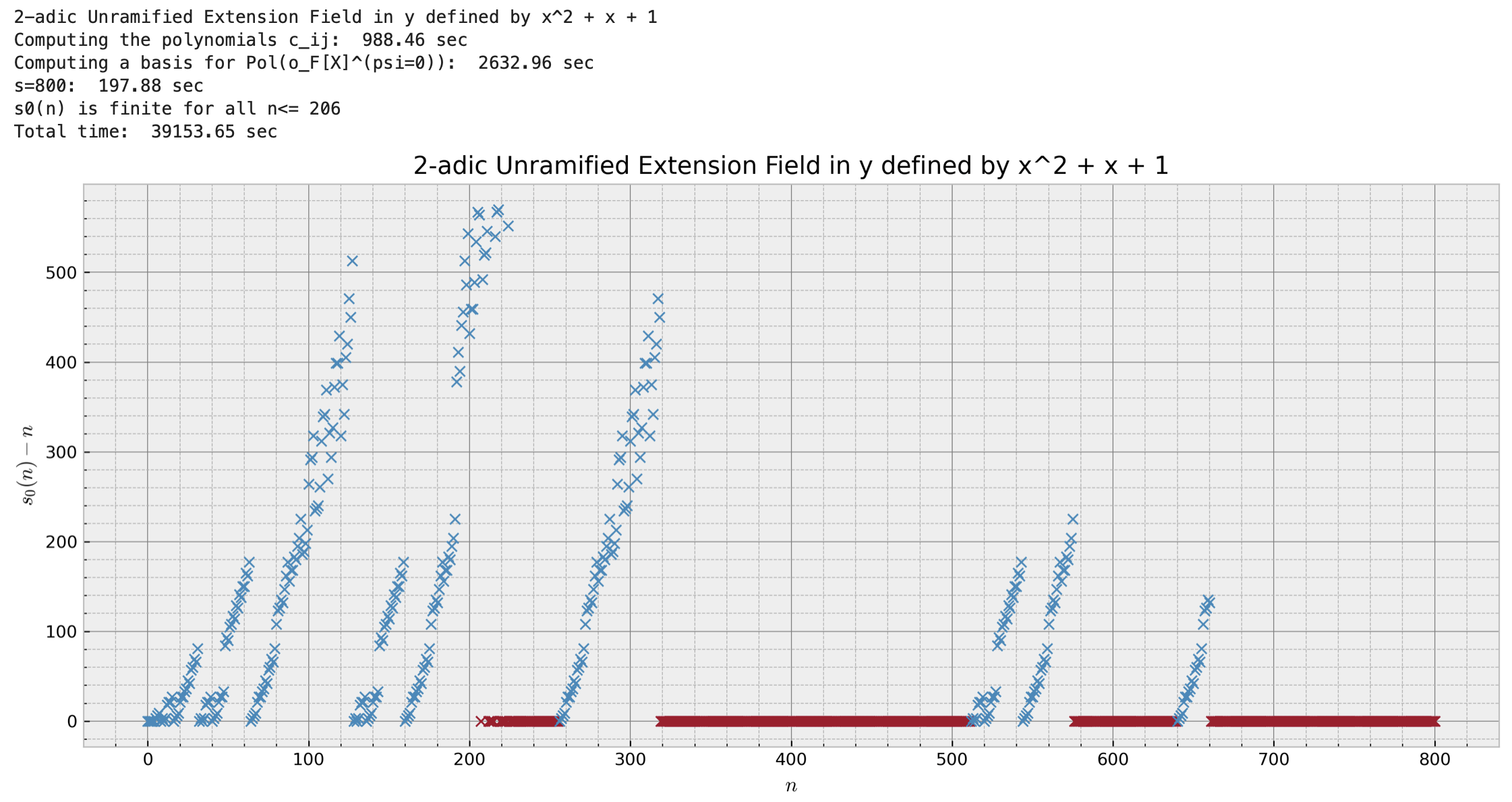
   Figure 1. Plot of $s_{0}(n)-n$ for $p=2$ and $N=800$. Red points are the $n$’s for which $s_{0}(n)=-1$.

2. For $p=3$ and $N=800$ and precision $6000$ we find that $s_{0}(n)$ is finite for $n\leq 226$

   

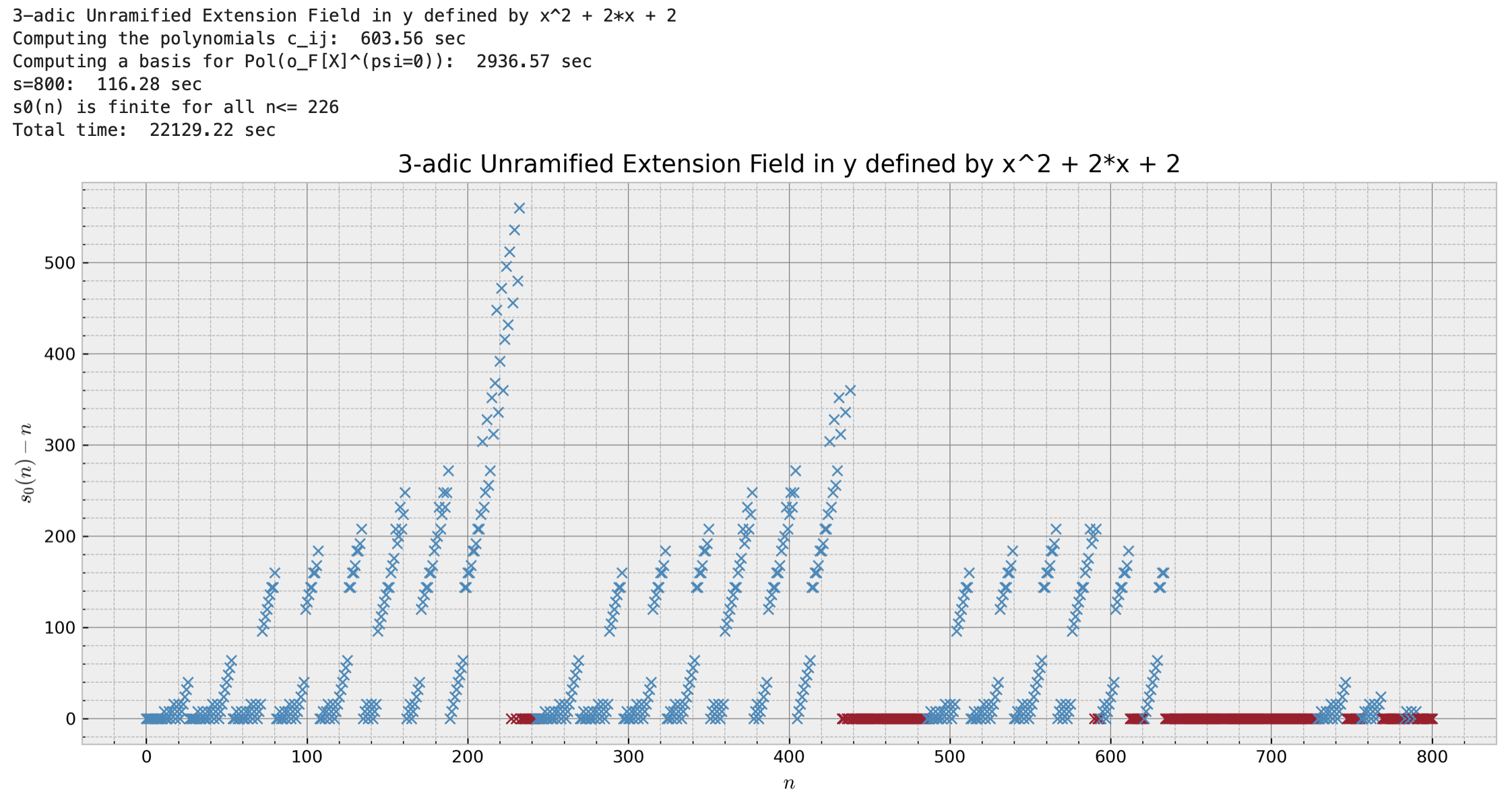
   Figure 2. Plot of $s_{0}(n)-n$ for $p=3$ and $N=800$. Red points are the $n$’s for which $s_{0}(n)=-1$.

Appendix A SageMath code

⬇

p=3 # prime number

N=120 # cutoff

precision = 1000 # p-adic precision

q=p^2 # Degree of the residue field

# Python imports

from time import process_time

import matplotlib.pyplot as plt

import numpy as np

# Definitions

import sage.rings.padics.padic_extension_generic

# Define the p-adic field, its ring of integers and the valuation function v

o_F.<y> = Zq(ZZ(q),prec=precision)

F.<y> = Qq(ZZ(q),prec=precision)

v = F.valuation()

print(F)

# Define the generator of the unique maximal ideal in o_F.

Pi = o_F(p)

# Do linear algebra over the ring of polynomials F[X]

# in one variable X with coefficients in the field F:

F_X.<X> = F[]

F_Y.<Y> = F[]

# Define the rings of power series over F and o_F and the Frobenius lift phi=pT+T^q.

F_T.<T>=PowerSeriesRing(F,default_prec=N)

phi_F=Pi*T+T^q

o_F_tt.<t>=PowerSeriesRing(o_F,default_prec=N)

phi=o_F_tt(phi_F(t))

def LogLT(N):

# Computes the logarithm of the Lubin-Tate formal group law with phi(T)=Pi*T+T^q up to precision O(T^(N+1))

h=[0,1]

for n in range(2,N+1):

h.append(sum([F(h[n-q*i+i]*binomial(n-q*i+i,i)*p^(n-q*i)) for i in range(1,floor((n)/q)+1)])/(p-p^n))

log_LT= sum([h[n]*T^n for n in range(1,N)])+O(T^(N+1))

return log_LT

def LogCarlemanMatrix(N):

# Computes the Carleman matrix of log_LT which is used for computing c_(i,j)

CMat = matrix(F,N+1,N+1)

# Compute the logarithm of the Lubin-Tate formal group law

log_LT=LogLT(N)

log_LT_j=F_T(1)

for j in range(0,N+1):

# Stores the coefficients of the power series log_LT(T)^j in row j of the matrix CMat

log_LT_dict_j=log_LT_j.dict()

l=[0 for _ in range(0,N+1)]

for key in log_LT_dict_j.keys():

l[key]=log_LT_dict_j[key]

for i in range(0,len(l)):

CMat[j,i]=l[i]

log_LT_j=log_LT_j*log_LT+O(T^(N+1))

return CMat

def BMatrix(N):

# BMatrix returns a square matrix B of size (N+1)x(N+1)

# such that B[i,0]+X*B[i,1]+...+X^N*B[i,N] for i=0...N forms

# an o_F-basis of the degree <=N part of o_F[X]^(psi=0)

# Create a list (genList) of all generators of o_F[X]^(psi=0) of degree at most N

genList=[]

for i in range(0,q-1):

phi_j=o_F_tt(1)

for j in range(0,N-i+1):

if i==0:

genList.append((Pi*t^(q-1)-(1-q))*phi_j+O(t^(N+1)))

else:

genList.append(t^i*phi_j+O(t^(N+1)))

phi_j=phi_j*phi

# Store the coefficients of the polynomials in genList in the matrix B

B=matrix(F,len(genList),N+1)

i=0

for gen in genList:

l=gen.list()

for j in range(0,len(l)):

B[i,j]=l[j]

i=i+1

# Perform Gaussian elimination

i0 = 0

for k in range(B.ncols()):

valuation_row_pairs = [

(v(B[i,k]), i) for i in range(i0, B.nrows()) if B[i,k] != 0]

if not valuation_row_pairs:

raise ValueError("B␣is␣not␣full-rank")

minv, i_minv = min(valuation_row_pairs)

# Swap the row of minimum valuation with the first bad row

B[i0, :], B[i_minv, :] = B[i_minv, :], B[i0, :]

# Divide the top row by a unit in o_F

u = B[i0, k] / Pi^int(v(B[i0, k]))

B[i0, :] /= u

# Cleave through the other rows

for i in range(i0 + 1, B.nrows()):

if v(B[i, k]) >= v(B[i0, k]):

B[i, :] -= B[i, k]/B[i0, k] * B[i0, :]

i0 += 1

# Return the first B.ncols() rows of the matrix B

return B[0:B.ncols(), :]

def CMatrix(N, D=None):

# Computes a matrix containing the polynomials c_(ij) using the Carleman matrix of log_LT

if D is None:

D = LogCarlemanMatrix(N)

# Define a diagonal matrix:

Diag = matrix(F_X, N+1,N+1, lambda x,y: kronecker_delta(x,y) * X^x)

# Compute the inverse of D:

S = D.inverse()

# Compute the matrix C:

C = S * Diag * D

return C

def w_q(n):

return (n - sum(n.digits(base=q))) / (q-1)

def compute_s(N, filename=None):

t_start = process_time()

D = LogCarlemanMatrix(N)

C = CMatrix(N, D)

t_end = process_time()

print(f"Computing␣the␣polynomials␣c_ij:␣{t_end-t_start␣:␣.2f}␣sec")

t_start = process_time()

# BPsi contains a basis of o_F[X]^(psi=0)_{<=N} of degree <=N

BPsi=BMatrix(N)

# Tau contains a basis of Pol(o_F[X]^{psi=0}_{<=N})

Tau=BPsi*C

t_end = process_time()

print(f"Computing␣a␣basis␣for␣Pol(o_F[X]^(psi=0)):␣{t_end-t_start␣:␣.2f}␣sec")

# s0_s[n] will store the minimal degree such that Int_n is contained in Pol(o_F[X]^{psi=0}_{<=s0_s[n]})

s0_s = [-1 for _ in range(N+1)]

B_old = Matrix(0,0)

d = 0

for s in range(N+1):

t_start = process_time()

# 1. Use the non-zero rows from previous calculations

# 2. Add a 0 column to its left

# 3. Add rows corresponding to entries from the j_th column of Tau_a

B = Matrix(F, 2*s-d+1, s-d+1)

B[0,0] = 1

B[1:s-d+1, 1:] = B_old

for i in [0 .. s-1]:

coeffs = Tau[i, s].list()

B[s-d+1+i, B.ncols()-len(coeffs)+d:] = vector(F, reversed(coeffs[d:]))

# Perform Gaussian elimination

i0 = 0

ks = []

for k in range(B.ncols()):

valuation_row_pairs = [

(v(B[i,k]), i) for i in range(i0, B.nrows()) if B[i,k] != 0]

if not valuation_row_pairs:

raise ValueError("B␣is␣not␣full-rank")

minv, i_minv = min(valuation_row_pairs)

ks.append(k)

# Swap the row of minimum valuation with the first bad row

B[i0, :], B[i_minv, :] = B[i_minv, :], B[i0, :]

# Divide the top row by a unit in o_F

u = B[i0, k] / Pi^int(v(B[i0, k]))

B[i0, :] /= u

# Cleave through the other rows

for i in range(i0 + 1, B.nrows()):

if v(B[i, k]) >= v(B[i0, k]):

B[i, :] -= B[i, k]/B[i0, k] * B[i0, :]

i0 += 1

d_is_updated = False

for b in [d .. s]:

n=b

# if the valuation of the leading coefficient is for the first time -w_q then store s in s0_s

if v(B[s-b, s-b]) == -w_q(n):

if s0_s[b] == -1:

s0_s[b] = s

else:

if not d_is_updated:

d = b

d_is_updated = True

B_old = B[:s-d+1, :s-d+1]

t_end = process_time()

print(f"s={s}:␣{t_end-t_start␣:␣.2f}␣sec", end=’\r’)

if filename is not None:

with open(filename, ’w’) as f:

f.write("n,s0\n")

for n, s0 in enumerate(s0_s):

f.write(f"{n},{s0}\n")

print()

# plot the result

plt.style.use(’bmh’)

fig = plt.figure(figsize=(15,6), dpi=300)

for n, s0 in enumerate(s0_s):

if s0 != -1:

plt.plot(n, s0-n, ’x’, c=’C0’)

else:

plt.plot(n, 0, ’x’, c=’C1’)

plt.xlabel(r"$n$")

plt.ylabel("$s_0(n)␣-␣n$")

plt.title(str(F))

plt.minorticks_on()

plt.grid(which=’both’)

plt.grid(which=’major’, linestyle=’-’, c=’grey’)

return s0_s, fig

t_start_tot = process_time()

s0_s = compute_s(N);

print("s0(n)␣is␣finite␣for␣all␣n<=",(s0_s[0]+[-1]).index(-1)-1)

t_end_tot = process_time()

print(f"Total␣time:␣{t_end_tot-t_start_tot␣:␣.2f}␣sec")

References

- [APZ98] V. Alexandru, N. Popescu and A. Zaharescu, On the closed subfields of , J. Number Theory 68 (1998), no. 2, 131–150.
- [Ard12] K. Ardakov, Prime ideals in nilpotent Iwasawa algebras, Invent. Math. 190 (2012), no. 2, 439–503.
- [AB24] K. Ardakov and L. Berger, Bounded functions on the character variety, Münster J. Math. (2024), to appear.
- [FX13] L. Fourquaux and B. Xie, Triangulable -analytic -modules of rank 2, Algebra Number Theory 7 (2013), no. 10, 2545–2592.
- [HMS14] Y. Hu, S. Morra and B. Schraen. Sur la fidélité de certaines représentations de sous une algèbre d’Iwasawa. Rend. Semin. Mat. Univ. Padova 131 (2014), 49–65.
- [Kap69] I. Kaplansky. Infinite abelian groups. Revised edition. University of Michigan Press, Ann Arbor, MI, 1969.
- [Kat77] N. M. Katz, Formal groups and -adic interpolation, Journées Arithmétiques de Caen (Univ. Caen, Caen, 1976), Astérisque No. 41–42, Soc. Math. France, Paris, 1977, pp. 55–65.
- [Kat81] N. M. Katz, Divisibilities, congruences, and Cartier duality, J. Fac. Sci. Univ. Tokyo Sect. IA Math. 28 (1981), no. 3, 667–678 (1982).
- [LT65] J. Lubin and J. Tate, Formal complex multiplication in local fields, Ann. of Math. (2) 81 (1965), 380–387.
- [ST01] P. Schneider and J. Teitelbaum, -adic Fourier theory, Doc. Math. 6 (2001), 447–481.
- [SI09] E. de Shalit and E. Iceland, Integer valued polynomials and Lubin-Tate formal groups, J. Number Theory 129 (2009), no. 3, 632–639.