Golden Ratio Mixing of Real and Synthetic Data for Stabilizing Generative Model Training

Abstract

Recent studies identified an intriguing phenomenon in recursive generative model training known as model collapse, where models trained on data generated by previous models exhibit severe performance degradation. Addressing this issue and developing more effective training strategies have become central challenges in generative model research. In this paper, we investigate this phenomenon theoretically within a novel framework, where generative models are iteratively trained on a combination of newly collected real data and synthetic data from the previous training step. To develop an optimal training strategy for integrating real and synthetic data, we evaluate the performance of a weighted training scheme in various scenarios, including Gaussian distribution estimation and linear regression. We theoretically characterize the impact of the mixing proportion and weighting scheme of synthetic data on the final model’s performance. Our key finding is that, across different settings, the optimal weighting scheme under different proportions of synthetic data asymptotically follows a unified expression, revealing a fundamental trade-off between leveraging synthetic data and generative model performance. Notably, in some cases, the optimal weight assigned to real data corresponds precisely to the reciprocal of the golden ratio. Finally, we validate our theoretical results on extensive simulated datasets and a real tabular dataset.

Keywords: Optimal Mixing, Generative Model, Golden Ratio, Model Collapse, Synthetic Data

1 Introduction

In recent years, synthetic data have been widely used to train generative models, especially in the domain of large language models (Meng et al.,, 2022; Shumailov et al.,, 2023; Dohmatob et al., 2024c, ) and computer vision (Man and Chahl,, 2022; Mishra et al.,, 2022). This trend is mainly motivated by the limited availability of data to train larger models due to neural scaling laws (Bansal et al.,, 2022; Villalobos et al.,, 2024). However, several critical issues arise regarding the utility of synthetic data for training purposes. For instance, because synthetic data do not perfectly align with the real data distribution, models trained on synthetic data are prone to have degraded performance. This phenomenon has been extensively validated in the literature (Xu et al.,, 2023; Wong et al.,, 2016; Dohmatob et al., 2024b, ).

A recent study by Shumailov et al., (2024) reveals that AI models may collapse when trained on recursively generated data. The recursive training framework is illustrated in Figure 1, where generative models are trained on synthetic data produced by earlier generative models. Over successive training iterations, these models gradually lose information about the real data distribution, a phenomenon known as model collapse. For example, Shumailov et al., (2024) use Gaussian distribution estimation to demonstrate how repeated estimation over iterations causes the estimated covariance matrix to almost surely collapse to zero, while the sample mean diverges. Similar results in a linear regression context are validated by Dohmatob et al., 2024a . In this paper, we refer to this framework (illustrated in Figure 1) as the fully synthetic framework.

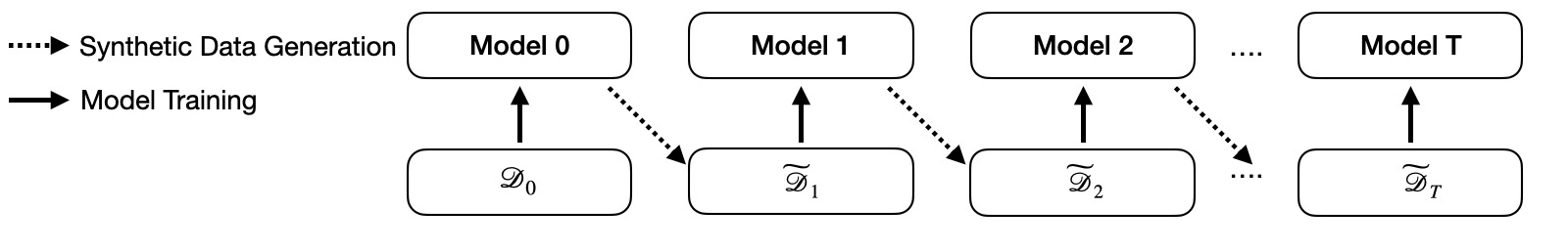
Figure 1: The general framework of model collapse phenomenon during recursive training (Shumailov et al.,, 2024). In this framework, $\mathcal{D}_{0}$ denotes the initial real dataset and $\widetilde{\mathcal{D}}_{t}$ denotes the synthetic dataset generated by the $(t-1)$-th generative model, which is then used to train the $t$-th generative model.

Subsequently, Gerstgrasser et al., (2024) and Kazdan et al., (2024) explore model collapse in a new scenario, illustrated in Figure 2, in which a model is trained iteratively, with each training step leveraging the original real training dataset $\mathcal{D}_{0}$ and all synthetic data in previous steps. Theoretically, they demonstrate that in both regression and Gaussian distribution estimation settings, the phenomenon of model collapse is avoided, showing that the expected test error remains bounded even as the number of iterations increases. In other words, model collapse is prevented by integrating all the data from previous steps into the training process. Furthermore, they demonstrate through experiments that data accumulation effectively prevents model collapse across various models, including LLMs and diffusion models. Later, such a data accumulation scheme is proved to be effective when the underlying generative models belong to exponential families (Dey and Donoho,, 2024). In this paper, we refer to this framework (illustrated in Figure 2) as the synthetic accumulation framework.

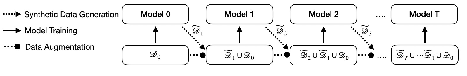
Figure 2: The general framework for mitigating the model collapse phenomenon during recursive training involves accumulating data (Gerstgrasser et al.,, 2024; Kazdan et al.,, 2024). In this framework, the training dataset is progressively expanded at each step $t$ by incorporating synthetic data from last generative model.

A key result of the synthetic accumulation framework is that it incorporates excessive synthetic data during training, leading to poorer performance in the final model compared to one trained purely on real data (Kazdan et al.,, 2024). In contrast, Bertrand et al., (2024) consider a data augmentation approach that utilizes only synthetic data generated by the most recent generative model, as shown in Figure 3. In this approach, the $t$-th generative model is trained on a combination of a fixed real dataset $\mathcal{D}_{0}$ and the synthetic dataset $\widetilde{\mathcal{D}}_{t-1}$ produced by the $(t-1)$-th generative model. Bertrand et al., (2024) show that this framework (Figure 3) can effectively avoid the model collapse phenomenon if the proportion of synthetic data is small. In this paper, we refer to this framework (illustrated in Figure 3) as the synthetic augmentation framework.

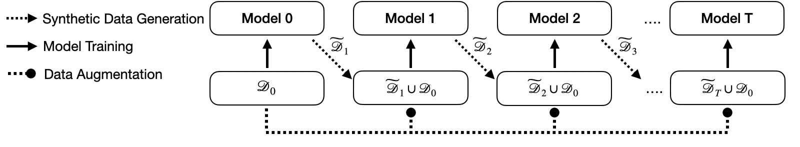
Figure 3: The general framework for avoiding the model collapse phenomenon during recursive training by augmenting only real data (Bertrand et al.,, 2024). In this framework, at the $t$-th training step, the generative model is trained based on $\widetilde{\mathcal{D}}_{t}\cup\mathcal{D}_{0}$.

The frameworks illustrated in Figures 1–3 all highlight a frustrating result: synthetic data fail to improve the performance of the final generative model, also empirically validated in this paper. Recently, Alemohammad et al., (2024) investigate the phenomenon of model collapse in a new scenario, where real data is continuously collected at each step for model estimation, as shown in Figure 4. In this work, the authors present empirical evidence demonstrating that a modest amount of synthetic data can enhance the performance of the final generative model. However, model performance declines when the amount of synthetic data exceeds a critical threshold. While Alemohammad et al., (2024) provide empirical evidence for the effectiveness of synthetic data within the framework illustrated in Figure 4, the underlying theoretical foundation remains unexplored. In this paper, we refer to this framework (illustrated in Figure 3) as the fresh data augmentation framework.

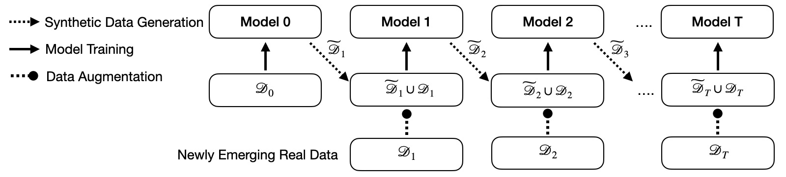
Figure 4: The general framework considered in this paper involves mixing newly collected real and synthetic data to address model collapse. In this framework, at the $t$-th training step, a newly collected dataset $\mathcal{D}_{t}$ is augmented with $\widetilde{\mathcal{D}}_{t}$ to train the $t$-th generative model.

In this paper, we theoretically investigate the phenomenon of model collapse within the new framework considered by Alemohammad et al., (2024). There are two primary practical reasons for studying the framework depicted in Figure 4. The first relates to privacy concerns. For instance, the California Consumer Privacy Act (CCPA) grants users the right to request that platforms retain their personal information only for a limited time. Consequently, in practical applications, the real dataset $\mathcal{D}_{0}$ may not always be available for future training as shown in the frameworks of Figures 1-3. Second, in a realistic setting, real data is continuously collected, enabling the training of new models using both synthetic data generated by prior models and newly collected real data. Despite its importance, the practice of training a model on a combination of newly collected real data and synthetic data from previous models remains theoretically underexplored. This naturally raises several critical questions:

• : Can mixing newly collected real data with synthetic data during training help prevent model collapse?

• : What is the optimal ratio of real to synthetic data when training a new generative model with data from the previous model?

• : To what extent can synthetic data enhance estimation efficiency?

To address these questions, we first introduce our definition of model collapse in parametric generative modeling (see Definition 1): statistical inconsistency of parameter estimation caused by the recursive training process. To mitigate this issue, we propose a weighted training scheme for generative models that integrates newly collected real data with varying amounts of synthetic data. We explore several scenarios involving recursive parameter estimation for Gaussian distributions and linear regression, building on previous research (Gerstgrasser et al.,, 2024; Kazdan et al.,, 2024; Bertrand et al.,, 2024). Our analysis demonstrates that the fresh data augmentation framework not only effectively prevents model collapse but also improves estimation efficiency. A comparison of different frameworks is provided in Table 1.

Table 1: The utility of synthetic data in different frameworks illustrated in Figures 1-4

Framework	Model collapse?	Synthetic data enhance estimation?
Fully Synthetic	✓	✗
Synthetic Accumulation	✗	✗
Synthetic Augmentation	✗	✗
Fresh Data Augmentation	✗	✓

In this paper, we summarize our contributions to the study of the model collapse phenomenon under the framework illustrated in Figure 4 as follows:

• Optimal Weight of Real and Synthetic Data: We explicate the optimal weights for real and synthetic data when training a new generative model using different amount of synthetic data across different regimes. Our findings reveal that while different regimes exhibit distinct model behaviors, the optimal weight asymptotically converges to a unified expression across all regimes. Interestingly, we find that regardless of the amount of real and synthetic data available in each round, simply mixing them without proper weighting is always suboptimal. In certain scenarios, we identify critical thresholds for the proportion of real and synthetic data in the mixture. As long as the weight of newly collected real data exceeds this threshold, model collapse can be effectively prevented.

• Surprising Connection to the Golden Ratio: When the amounts of real and synthetic data remain the same in each training iteration, we make a striking discovery: the optimal weight of real data is the reciprocal of the golden ratio.

• Threshold for Beneficial Synthetic Data: We demonstrate that as long as the weight of synthetic data in each iteration remains below a certain threshold, incorporating synthetic data enhances estimation efficiency in our fresh data augmentation setting compared to using only real data, highlighting the effectiveness of incorporating synthetic data for training.

The rest of this paper is organized as follows. In Section 2, we introduce the necessary notations and provide background on model collapse within a parametric setting. In Section 3, we explore the model collapse phenomenon within the fresh data augmentation framework, focusing on Gaussian estimation, and develop optimal training schemes to avoid model collapse and enhance estimation efficiency. In Section 4, we extend the analysis in Section 3 to linear regression. In Section 5, we discuss the selection of the optimal ratio between real and synthetic data from a practical perspective, taking into account the cost of data acquisition. In Section 6, we conduct extensive simulations and a real application to validate our theoretical findings. In Section 7, we explore potential future extensions of this work. Additional contents and all proofs are deferred to the Appendix.

2 Preliminaries

In this section, we first introduce the necessary notations in Section 2.1. To formalize our analysis, we then provide a mathematical definition of model collapse within the framework of parametric model estimation in Section 2.2. While model collapse was originally observed in the training of AI models (Shumailov et al.,, 2024), a formal mathematical definition within the broader context of estimating parametric generative models remains absent.

2.1 Notations

In this paper, we use bold notation to represent multivariate quantities and unbolded notation for univariate quantities. For any positive integer $M$, we define $[M]$ as the set $[M]=\{1,2,\ldots,M\}$. For example, $\bm{x}\in\mathbb{R}^{p}$ represents a $p$-dimensional vector, while $x$ represents a real value. For a vector $\bm{x}\in\mathbb{R}^{p}$, we denote its $l_{2}$-norm as $\|\bm{x}\|_{2}=\big{(}\sum_{i=1}^{p}|x_{i}|^{2}\big{)}^{1/2}$. For a continuous random variable $X$, we let $P_{X}(x)$ denote its probability density function at $x$ and $\mathbb{P}_{X}$ denote the associated probability measure. We use $\mathbb{E}_{X}$ to denote the expectation taken with respect to the randomness of $X$. For a sequence of random variables $\{X_{n}\}_{n\in\mathbb{N}}$, we write $X_{n}=o_{p}(1)$ to indicate that $X_{n}$ converges to zero in probability. For a matrix $\bm{A}=(A_{ij})_{i,j\in[n]}$, we define its trace as $\text{tr}(\bm{A})=\sum_{i=1}^{n}A_{ii}$. Finally, we use $\mathcal{F}_{t}$ to represent the $\sigma$-algebra generated by all events occurring up to the $t$-th training step.

2.2 Model Collapse in Parametric Generative Models

In this section, we present a general definition of model collapse for parametric generative models within the framework of recursive model estimation as illustrated in Figure 5. Consider a family of generative models parameterized by $\bm{\theta}\in\bm{\Theta}$, denoted as $\{\mathbb{P}(\cdot\mid\bm{\theta})\mid\bm{\theta}\in\bm{\Theta}\}$. Let $\bm{\theta}^{\star}$ be the ground truth parameter. The goal is to estimate $\bm{\theta}^{\star}$ after successive iterations.

Figure 5: The general framework of recursive model estimation.

In the framework of Figure 5, an estimation scheme $\mathcal{M}:\mathcal{X}^{\mathbb{N}}\to\bm{\Theta}$ is applied consistently at each estimation step, i.e., $\widehat{\bm{\theta}}_{t}=\mathcal{M}(D_{t})$ for $t\geq 0$, where $\mathcal{X}$ represents the data support, $\bm{\Theta}$ denotes the parameter space, and $D_{t}=\{\bm{x}_{t,i}\}_{i=1}^{N_{t}}$ is the dataset used at step $t$. Aligning with the frameworks in Figure 1-4, we define $D_{0}=\{\bm{x}_{0,i}\}_{i=1}^{N_{0}}$ as a real dataset drawn from $\mathbb{P}(\bm{x}\mid\bm{\theta}^{\star})$. For $t\geq 1$, $D_{t}$ may consist of either real data or synthetic data generated by previous generative models $\{\mathbb{P}(\bm{x}\mid\widehat{\bm{\theta}}_{i}):0\leq i\leq t-1\}$. Without loss of generality, we assume that the sample sizes $\{N_{t}\}_{t=0}^{\infty}$ follow the pattern $N_{t}=N_{0}\times c_{t}$ for $t\geq 1$. In other words, given a fixed initial real sample size $N_{0}$, the sequence $\{c_{t}\}_{t=1}^{\infty}$ determines the trend of the training datasets throughout the training process.

We denote by $\mathbb{P}_{t}(\bm{x})$ the underlying distribution of $D_{t}=\{\bm{x}_{t,i}\}_{i=1}^{N_{t}}$. Since $D_{t}$ consists of both real data and synthetic data generated by previous models, $\mathbb{P}_{t}(\bm{x})$ is a mixture of the real data distribution $\mathbb{P}(\bm{x}\mid\bm{\theta}^{\star})$ and the synthetic data distributions $\{\mathbb{P}(\bm{x}\mid\widehat{\bm{\theta}}_{i}):0\leq i\leq t-1\}$ prior to the $t$-th step. In other words, the dependence of $\mathbb{P}_{t}(\bm{x})$ on $\mathbb{P}(\bm{x}\mid\bm{\theta}^{\star})$ and $\{\mathbb{P}(\bm{x}\mid\widehat{\bm{\theta}}_{i}):0\leq i\leq t-1\}$ is determined by the strategy used to integrate synthetic and real data for training. For example, in a fully synthetic framework, the distribution simplifies to $\mathbb{P}_{t}(\bm{x})=\mathbb{P}(\bm{x}\mid\widehat{\bm{\theta}}_{t-1})$. In contrast, under a synthetic data augmentation framework, it follows $\mathbb{P}_{t}(\bm{x})=\frac{1}{2}\mathbb{P}(\bm{x}\mid\widehat{\bm{\theta}}_{t-1})+\frac{1}{2}\mathbb{P}(\bm{x}\mid\bm{\theta}^{\star})$.

Notably, the framework in Figure 5 generalizes those in Figures 1-4 as special cases. Particularly, the framework in Figure 5 simplifies to the fully-synthetic case in Figure 1 when $N_{i}=N_{j}$ for all $i,j\geq 0$, and $\{\bm{x}_{t,i}\}_{i=1}^{N_{t}}$ is entirely sampled from $\mathbb{P}(\bm{x}\mid\widehat{\bm{\theta}}_{t-1})$, i.e., $\mathbb{P}_{t}(\bm{x})=\mathbb{P}(\bm{x}\mid\widehat{\bm{\theta}}_{t-1})$ for $t\geq 1$.

The key challenge in Figure 5 is to assess the performance of the final generative model $\mathbb{P}(\cdot\mid\widehat{\bm{\theta}}_{T})$ when $T$ is large, which can be quantified by the estimation error $\mathbb{E}\|\widehat{\bm{\theta}}_{T}-\bm{\theta}^{\star}\|_{2}^{2}$. Here, the expectation is taken with respect to the randomness of all previous training datasets. If $N_{0}$ is fixed, the performance of $\widehat{\bm{\theta}}_{T}$ in estimating $\bm{\theta}^{\star}$ as $T\to\infty$ is influenced by three key factors: (1) the estimation scheme $\mathcal{M}(\cdot)$, (2) the pattern of sample sizes $\{c_{t}\}_{t=1}^{\infty}$, and (3) the underlying distribution $\mathbb{P}_{t}$ at each step. In other words, once $(\mathcal{M},\{c_{t}\}_{t=1}^{\infty},\{\mathbb{P}_{t}\}_{t=1}^{\infty})$ is specified, the training strategy for recursive estimation is uniquely determined.

In statistical learning theory, if $(\mathcal{M},\{c_{t}\}_{t=1}^{\infty},\{\mathbb{P}_{t}\}_{t=1}^{\infty})$ is fixed with an appropriate estimation scheme $\mathcal{M}$, the error $\mathbb{E}\|\widehat{\bm{\theta}}_{T}-\bm{\theta}^{\star}\|_{2}^{2}$ for a fixed $T$ should converge to zero as $N_{0}$ increases to infinity. However, existing literature (Shumailov et al.,, 2024; Kazdan et al.,, 2024) shows that, as $T$ increases, $\widehat{\bm{\theta}}_{T}$ gradually loses information about $\mathbb{P}(\cdot|\bm{\theta}^{\star})$ and finally fails to converge to $\bm{\theta}^{\star}$ regardless of the size of data during recursive training process. Therefore, preventing model collapse should focus on designing appropriate data integration and training schemes to ensure that the estimation error $\mathbb{E}\|\widehat{\bm{\theta}}_{T}-\bm{\theta}^{\star}\|_{2}^{2}$ remains stable as $T$ grows to infinity and decreases as more data is used for training. Based on this rationale, we formally define model collapse in the context of parametric generative models in Definition 1.

Definition 1 (Model Collapse in Parametric Generative Models).

For a recursive training scheme $(\mathcal{M},\{c_{t}\}_{t=1}^{\infty},\{\mathbb{P}_{t}\}_{t=1}^{\infty})$, we say that model collapse occurs if there exists a constant $\delta>0$ such that $\lim\limits_{T\to\infty}\mathbb{E}\|\widehat{\bm{\theta}}_{T}-\bm{\theta}^{\star}\|_{2}^{2}\geq\delta$ for any value of $N_{0}$.

In Definition 1, model collapse refers to the phenomenon where the estimator $\widehat{\bm{\theta}}$ progressively loses information about the true data distribution $\mathbb{P}(\cdot|\bm{\theta}^{\star})$ as $T$ increases, causing $\widehat{\bm{\theta}}$ to fail to converge to $\bm{\theta}^{\star}$ regardless of the samples used throughout the training process. We characterize this failure by the estimator’s inconsistency, independent of the sample sizes used at each estimation step. Specifically, the limiting error $\lim_{T\rightarrow\infty}\mathbb{E}\|\widehat{\bm{\theta}}_{T}-\bm{\theta}^{\star}\|_{2}^{2}$ remains bounded away from zero, no matter how large the sample sizes are at any step.

3 Gaussian Distribution Estimation

In this section, we investigate the phenomenon of model collapse within the fresh data augmentation framework, using recursive Gaussian distribution estimation as a case study. We analyze the univariate case in this section, which is subsequently extended to the multivariate case in Appendix A.1.

Within the fresh data augmentation framework, the process begins with a real dataset $\mathcal{D}_{0}=\{x_{0,i}\}_{i=1}^{n}$ sampled from $N(\mu,\sigma^{2})$. At the $t$-th training step for $t\geq 1$, a newly collected real dataset $\mathcal{D}_{t}=\{x_{t,i}\}_{i=1}^{n}$ is drawn from $N(\mu,\sigma^{2})$, and a synthetic dataset $\widetilde{\mathcal{D}}_{t}=\{\widetilde{x}_{t,i}\}_{i=1}^{m}$ is generated based on the $(t-1)$-th Gaussian distribution. As a result, the training dataset at step $t$ is $D_{t}=\mathcal{D}_{t}\cup\widetilde{\mathcal{D}}_{t}$. As illustrated in Figure 4, $\mathcal{D}_{t}$ and $\widetilde{\mathcal{D}}_{t}$ are used to estimate the parameters of a univariate Gaussian distribution at the $t$-th step. Although the most straightforward approach might be to simply combine the two datasets for training, we show in Remark 1 that at least in the case of mean estimation, this method is strictly suboptimal. Instead, we adopt a weighted estimation scheme as follows:

Mean Estimation: $$\mu_{t}(w,k)=\mathop{\mathrm{argmin}}_{\mu\in\mathbb{R}}\frac{w}{n}\sum_{i=1}^{n}(\mu-x_{t,i})^{2}+\frac{1-w}{m}\sum_{i=1}^{m}(\mu-\widetilde{x}_{t,i})^{2},$$ (1)

Variance Estimation: $$\sigma_{t}^{2}(w,k)=\mathop{\mathrm{argmin}}_{\sigma^{2}\in\mathbb{R}}w(\sigma^{2}-\widehat{S}_{t})^{2}+(1-w)(\sigma^{2}-\widetilde{S}_{t})^{2},$$ (2)

where $k=\frac{n}{m}$ represents the ratio of real data size to synthetic data size, and $\widehat{S}_{t}=\frac{1}{n-1}\sum_{i=1}^{n}(x_{t,i}-\widehat{\mu}_{t})^{2}$ and $\widetilde{S}_{t}=\frac{1}{m-1}\sum_{i=1}^{m}(\widetilde{x}_{t,i}-\widetilde{\mu}_{t})^{2}$ denote the sample variances of the real and synthetic data at the $t$-th step, respectively. Here, $\widehat{\mu}_{t}=\frac{1}{n}\sum_{i=1}^{n}x_{t,i}$ and $\widetilde{\mu}_{t}=\frac{1}{m}\sum_{i=1}^{m}\widetilde{x}_{t,i}$ are the sample means of the real and synthetic data, respectively.

The overall recursive estimation process for a univariate Gaussian distribution, obtained by solving (1), is summarized in Fresh Data Augmentation Case 1. In this process, $w$ is a weighting parameter that controls the emphasis placed on the real data in the optimization process. We assume that $w$ is fixed throughout the entire recursive training process. Specifically, $w=0$ corresponds to the fully synthetic framework depicted in Figure 1, while $w=1$ refers to the scenario that only utilizes real data at the $t$-th step. Additionally, $k$ is a parameter controlling the size of synthetic data used for estimation. In practice, $k$ can be extremely small, indicating that a large amount of synthetic data is used for training. From a statistical viewpoint, assuming $n$ is fixed, the resulting estimators in the case of $k=0$ are optimal in terms of estimation efficiency. However, the choice of $k$ usually depends on the tradeoff between the cost of computational resources and estimation improvement in some real generative modeling scenarios.

Algorithm 1 - Univariate Gaussian Estimation

 Initialization: Compute $\mu_{0}=\frac{1}{n}\sum_{i=1}^{n}x_{0,i}$ and $\sigma_{0}^{2}=\frac{1}{n-1}\sum_{i=1}^{n}(x_{0,i}-\mu_{0})^{2}$ based on $\mathcal{D}_{0}=\{x_{0,i}\}_{i=1}^{n}$ from $N(\mu,\sigma^{2})$;

 for $t=1,2,\ldots,T$ do

  1. Data Collection: Sample $\widetilde{\mathcal{D}}_{t}=\{\widetilde{x}_{t,i}\}_{i=1}^{m}$ from $N(\mu_{t-1},\sigma_{t-1}^{2})$ and collect a new real dataset $\mathcal{D}_{t}=\{x_{t,i}\}_{i=1}^{n}$ from $N(\mu,\sigma^{2})$;

  2. Mean Estimation: Compute the mean of the Gaussian distribution at the $t$-th training step:

$$\mu_{t}(w,k)=w\widehat{\mu}_{t}+(1-w)\widetilde{\mu}_{t},$$

where $\widehat{\mu}_{t}=\frac{1}{n}\sum_{i=1}^{n}x_{t,i}$ and $\widetilde{\mu}_{t}=\frac{1}{m}\sum_{i=1}^{m}\widetilde{x}_{t,i}$.

  3. Variance Estimation: Compute the variance of the Gaussian distribution at the $t$-th training step:

$$\sigma_{t}^{2}(w,k)=w\widehat{S}_{t}+(1-w)\widetilde{S}_{t},$$

where $\widehat{S}_{t}=\frac{1}{n-1}\sum_{i=1}^{n}(x_{t,i}-\widehat{\mu}_{t})^{2}$ and $\widetilde{S}_{t}=\frac{1}{m-1}\sum_{i=1}^{m}(\widetilde{x}_{t,i}-\widetilde{\mu}_{t})^{2}$.

 end for

 return  $\mu_{T}$ and $\sigma_{T}^{2}$.

To analyze the behavior of $\mu_{t}(w,k)$ and $\sigma_{t}^{2}(w,k)$ as $t\to\infty$ with $k\triangleq n/m$ being the mixing ratio, we define the following metrics:

$$\text{Err}(\mu_{t}(w,k))=\mathbb{E}\big{[}(\mu_{t}(w,k)-\mu)^{2}\big{]}\mbox{ and }\text{Err}(\sigma_{t}^{2}(w,k))=\mathbb{E}\big{[}(\sigma_{t}^{2}(w,k)-\sigma^{2})^{2}\big{]},$$

where $\text{Err}(\mu_{t}(w,k))$ and $\text{Err}(\sigma_{t}^{2}(w,k))$ represent the expected squared errors of $\mu_{t}(w,k)$ and $\sigma_{t}^{2}(w,k)$, measuring the estimation errors for $\mu_{t}(w,k)$ and $\sigma_{t}^{2}(w,k)$, respectively. It is important to note that these expectations are taken with respect to the randomness inherent in all real and synthetic datasets generated during the first $t$ steps. Essentially, $\{\mu_{t}(w,k)\}_{t=1}^{T}$ and $\{\sigma_{t}^{2}(w,k)\}_{t=1}^{T}$ can be regarded as two time series, where the randomness of $(t-1)$-th element is contained within that of $t$-th element. A key problem is analyzing the behavior of $\mu_{t}(w,k)$ and $\sigma_{t}^{2}(w,k)$ as $t$ approaches infinity. Therefore, we consider the following metrics for the case where $t=\infty$:

$$\mathrm{Err}(\mu_{\infty}(w,k))\triangleq\lim_{t\rightarrow\infty}\mathrm{Err}\left(\mu_{t}(w,k)\right)\mbox{ and }\mathrm{Err}(\sigma_{\infty}^{2}(w,k))\triangleq\lim_{t\rightarrow\infty}\mathrm{Err}\left(\sigma_{t}^{2}(w,k)\right).$$

In the following, we investigate the behavior of $\mathrm{Err}(\mu_{\infty}(w,k))$ and $\mathrm{Err}(\sigma_{\infty}^{2}(w,k))$ in a finite-sample setting, aiming to shed light on the impact of $w$ and $k$.

Theorem 1.

For any $w\in(0,1]$ and $n,m\geq 1$ with $k=\frac{n}{m}$. It holds that

$$\mathrm{Err}(\mu_{\infty}(w,k))=\lim_{t\rightarrow\infty}\mathrm{Err}(\mu_{t}(w,k))=\frac{C(w,k)\sigma^{2}}{n},$$

where $C(w,k)=\frac{w^{2}+(1-w)^{2}k}{2w-w^{2}}$. Using the optimal weighting parameter $w^{\star}=\frac{\sqrt{k^{2}+4k}-k}{2}$ with $w^{\star}=\mathop{\mathrm{argmin}}\limits_{w\in(0,1]}C(w,k)$, the estimation improvement for estimating $\mu$ is given by

$$\frac{\mathrm{Err}(\mu_{\infty}(w^{\star},k))}{\mathrm{Err}(\mu_{\infty}(1,k))}=w^{\star}=\frac{\sqrt{k^{2}+4k}-k}{2}<1.$$

Particularly, when $k=1$ (n=m), we have $\mathrm{Err}(\mu_{\infty}(w,1))<\mathrm{Err}(\mu_{\infty}(1,1))$ for any $w\in(\frac{1}{3},1)$.

In Theorem 1, we derive explicit expressions for $\mathrm{Err}(\mu_{\infty}(w,k))$ under different values of the weighting parameter $w$ and the mixing ratio $k$. Specifically, we show that the finite sample $l_{2}$-error of $\mu_{t}(w,k)$ in estimating $\mu$ is given by $\frac{C(w,k)\sigma^{2}}{n}$ when $t$ approaches infinity, where $C(w,k)$ depends on $w$ and $k\triangleq\frac{n}{m}$, the ratio of real to synthetic data generated in each round. Furthermore, we compare the estimation errors of our proposed estimator with optimal weight $w^{\star}$ and the estimator based solely on newly emerging real samples in each round. Interestingly, we find that the ratio of their estimation errors is exactly $w^{\star}$, which is always less than 1, as shown in Figure 6. Clearly, as more synthetic data is integrated during the estimation process (i.e., smaller values of $k$), the estimation accuracy improves. In particular, as $k$ approaches 0 (representing an infinite number of synthetic samples), $\mathrm{Err}(\mu_{\infty}(w^{\star},k))$ converges to zero, implying that the proposed estimator converges to $\mu$ after recursive estimation. Additionally, we demonstrate the existence of a phase transition phenomenon in $\mathrm{Err}(\mu_{\infty}(w,k))$ depending on the choice of $w$. In particular, when $n=m$ (see Left Panel of Figure 6), $\mathrm{Err}(\mu_{\infty}(w,k))$ is smaller than the estimation error $\mathrm{Err}(\mu_{\infty}(1,1))$ that relies solely on newly collected real data, provided that $w$ is chosen to be greater than $1/3$. Conversely, when $w$ is smaller than $1/3$, $\mu_{\infty}(w,1)$ performs worse than $\mu_{\infty}(1,1)$ in estimating $\mu$.

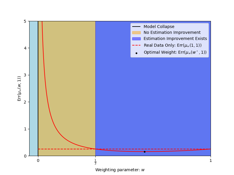
(a) Phase Transition of $\mathrm{Err}(\mu_{\infty}(w,1))$

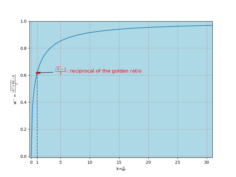
(b) The Optimal Weighting $w^{\star}$ for Varying $k$

Figure 6: The left panel illustrates the quantitative behavior of $\mathrm{Err}(\mu_{\infty}(w,k))$ with $n=m=4$ across three phases: (1) the model collapse phase, (2) the phase with no estimation improvement, and (3) the phase with estimation improvement. The right panel demonstrates the quantitative relationship between the optimal weight $w^{\star}$ and the mixing ratio $k$ is presented. Particularly, when $n=m$ (i.e., $k=1$), $w^{\star}$ is the reciprocal of the golden ratio.

Corollary 1.

$\mathrm{Err}(\mu_{\infty}(1,k))$ exhibits the following special cases:

• Fully Synthetic - Model Collapse: $\lim_{w\rightarrow 0^{+}}\mathrm{Err}(\mu_{\infty}(w,k))=\infty$ for any $k>0$,

• Real Data Only: $\mathrm{Err}(\mu_{\infty}(1,k))=\frac{\sigma^{2}}{n}$ for any $k>0$,

• Optimal Weight: $\mathrm{Err}(\mu_{\infty}(w^{\star},k))=\frac{w^{\star}\sigma^{2}}{n}$ for any $k>0$,

where $w^{\star}=\frac{\sqrt{k^{2}+4k}-k}{2}$ is the optimal weight as defined in Theorem 1.

In Corollary 1, we present several special cases of Theorem 1. Notably, when $w=0$ (corresponding to the fully synthetic case), the estimation error $\mathrm{Err}(\mu_{\infty}(w,k))$ diverges to infinity. This finding aligns with existing literature on model collapse in Gaussian mean estimation (Kazdan et al.,, 2024; Shumailov et al.,, 2024). Interestingly, when $m=n$, the minimal estimation error occurs at $w=w^{\star}=\frac{-1+\sqrt{5}}{2}$, the reciprocal of the golden ratio $\frac{1+\sqrt{5}}{2}$. Using this optimal weight, the estimation error $\mathrm{Err}(\mu_{\infty}(w,k))$ improves compared to using only real data, as evidenced by $\frac{\sqrt{k^{2}+4k}-k}{2}<1$ for any $k>0$. Specifically, when $k=1$ ($n=m$), the improvement is given by $\frac{\mathrm{Err}(\mu_{\infty}(w^{\star},1))}{\mathrm{Err}(\mu_{\infty}(1,1))}=w^{\star}=\frac{\sqrt{5}-1}{2}$.

In Theorem 1, we consider a special case where each synthetic sample is assigned the same weight internally, so does each real sample. However, in a more general setting, where each synthetic sample $\widetilde{x}_{t,i}$ has an associated weight $\widetilde{w}_{i}$ and each real sample ${x}_{t,i}$ has a weight $w_{i}$, we can extend the proof technique of Theorem 1 to show that the proposed weighted combination in Theorem 1 remains the Best Linear Unbiased Estimator (BLUE), as stated in the following proposition.

Proposition 1.

Consider a more general update rule for mean estimation given by:

$${\mu}_{t}(\{w_{i}\}_{i=1}^{n},\{\widetilde{w}_{j}\}_{j=1}^{m},k)=\frac{1}{n}\sum_{i=1}^{n}w_{i}{x}_{t,i}+\frac{1}{m}\sum_{j=1}^{m}\widetilde{w}_{j}{x}_{t,i},$$ (3)

where $w_{i}$ and $\widetilde{w}_{j}$ are the weights assigned to the $i$-th real and the $j$-th synthetic data points, respectively, satisfying that $\sum_{i=1}^{n}w_{i}/n+\sum_{j=1}^{m}\widetilde{w}_{j}/m=1$. Consider the limiting estimation error defined as

$$\mathrm{Err}({\mu}_{\infty}(\{w_{i}\}_{i=1}^{n},\{\widetilde{w}_{j}\}_{j=1}^{m},k))=\lim_{t\rightarrow\infty}\mathbb{E}\big{[}\|{\mu}_{t}(\{w_{i}\}_{i=1}^{n},\{\widetilde{w}_{j}\}_{j=1}^{m},k)-{\mu}\|_{2}^{2}\big{]}.$$

It holds true that $\mathrm{Err}(\bm{\mu}_{\infty}(\{w_{i}\}_{i=1}^{n},\{\widetilde{w}_{j}\}_{j=1}^{m},k))$ is minimized by $w_{i}=w^{\star}$ for $i\in[n]$ and $\widetilde{w}_{j}=1-w^{\star}$ for $j\in[m]$, where $w^{\star}=\frac{\sqrt{k^{2}+4k}-k}{2}$ as defined in Theorem 1.

Remark 1 (The Advantage of Weighted Training Over Direct Mixing).

The primary reason for adopting a weighted training scheme over direct mixing is that simply combining the data without explicit weighting can be strictly suboptimal. For example, consider the mean estimation step. If we directly merge the datasets $\mathcal{D}_{t}$ and $\widetilde{\mathcal{D}}_{t}$ and minimize the empirical loss on them:

$${\mu}_{t}(w,k)=\mathop{\mathrm{argmin}}_{{\mu}\in\mathbb{R}^{p}}\frac{1}{n+m}\left\{\sum_{i=1}^{n}\|{\mu}-{x}_{t,i}\|_{2}^{2}+\sum_{i=1}^{m}\|{\mu}-\widetilde{{x}}_{t,i}\|_{2}^{2}\right\},$$

then the resulting estimate can be written as ${\mu}_{t}(w_{0},k)=w_{0}\widehat{{\mu}}_{t}+(1-w_{0})\widetilde{{\mu}}_{t}$, where the implicit weight $w_{0}$ is given by:

$$w_{0}=\frac{n}{n+m}=\frac{2k}{k+2+k}=\frac{2k}{\sqrt{k^{2}+4k+4}+k}<w^{\star}=\frac{\sqrt{k^{2}+4k}-k}{2}=\frac{2k}{\sqrt{k^{2}+4k}+k}.$$

A detailed derivation is provided in Appendix. A.2. This inequality shows that directly mixing the data results in a strictly suboptimal weight for mean estimation for any value of $k$. The proposed weighted training scheme achieves a better balance between real and synthetic data.

Theorem 2.

For any $w\in(0,1]$, $n,m\geq 2$, and $k>0$, it holds that

$$\mathrm{Err}(\sigma_{\infty}^{2}(w,k))=\begin{cases}\infty,&0<w\leq 1-\sqrt{\frac{m-1}{m+1}},\\[10.0pt] C_{1}(w,m,n)\sigma^{4},&1-\sqrt{\frac{m-1}{m+1}}<w\leq 1,\end{cases}$$

where $C_{1}(w,m,n)=\frac{w^{2}\left(1+\frac{2}{n-1}\right)+2w(1-w)}{1-(1-w)^{2}\left(1+\frac{2}{m-1}\right)}-1$. The optimal weight $w^{\star}=\mathop{\mathrm{argmin}}_{w\in(0,1]}C_{1}(w,m,n)$ is given as

$$w^{\star}=\frac{\sqrt{n^{2}+\left(4m-2\right)n-4m+5}-n+3}{2m+2}.$$

Particularly, when $m,n\rightarrow\infty$ with $\frac{n}{m}=k$, $w^{\star}\rightarrow\frac{\sqrt{k^{2}+4k}-k}{2}$. The estimation improvement exists in the following cases:

$$\frac{\mathrm{Err}\big{(}\sigma_{\infty}^{2}(w,k)\big{)}}{\mathrm{Err}(\sigma_{\infty}^{2}(1,k))}<1,\text{ for any }w\in\left(\frac{n+1}{n+2m-1},1\right),$$

$$\lim_{n,m\rightarrow\infty,\frac{n}{m}\rightarrow k} \frac{\mathrm{Err}\big{(}\sigma_{\infty}^{2}(w^{\star},k)\big{)}}{\mathrm{Err}(\sigma_{\infty}^{2}(1,k))}=\frac{\sqrt{k^{2}+4k}-k}{2}<1,\text{ for any }k\in\mathbb{R}_{\geq 0},$$

$$\lim_{m\rightarrow\infty} \frac{\mathrm{Err}\big{(}\sigma_{\infty}^{2}(w,k)\big{)}}{\mathrm{Err}(\sigma_{\infty}^{2}(1,k))}=\frac{w^{2}}{2w-w^{2}}<1,\text{ for any }w\in\left(1-\sqrt{\frac{m-1}{m+1}},1\right].$$

In Theorem 2, we derive the explicit form of $\mathrm{Err}(\sigma_{\infty}^{2}(w,k))$ for different values of the weighting parameter $w$ and the mixing ratio $k$. Notably, $\mathrm{Err}(\sigma_{\infty}^{2}(w,k))$ exhibits distinct behavior compared to $\mathrm{Err}(\mu_{\infty}(w,k))$. Specifically, our proposed estimator $\sigma_{t}^{2}(w,k)$ undergoes a phase transition in estimating $\sigma^{2}$. When $w\leq 1-\sqrt{\frac{m-1}{m+1}}$, the estimation error $\mathrm{Err}(\sigma_{\infty}^{2}(w,k))$ diverges to infinity, indicating that the estimator is inconsistent, regardless of the number of real and synthetic samples used. This result suggests that model collapse persists when $w$ is too small, demonstrating that it can occur even when real data is incorporated into training. In contrast, when $w>1-\sqrt{\frac{m-1}{m+1}}$, the estimation error remains finite and depends on the real and synthetic sample sizes. To achieve better estimation performance than using only newly emerging real data, $w$ should be set higher than $\frac{n+1}{n+2m-1}$. Furthermore, as $n$ and $m$ approach infinity with $n/m=k$, the optimal weight $w^{\star}$ aligns with that for $\mathrm{Err}(\mu_{\infty}(w,k))$, and $\mathrm{Err}(\sigma_{\infty}^{2}(w,k))$ achieves the same estimation improvement as $\mathrm{Err}(\mu_{\infty}(w,k))$ compared to the estimator based solely on newly emerging real samples.

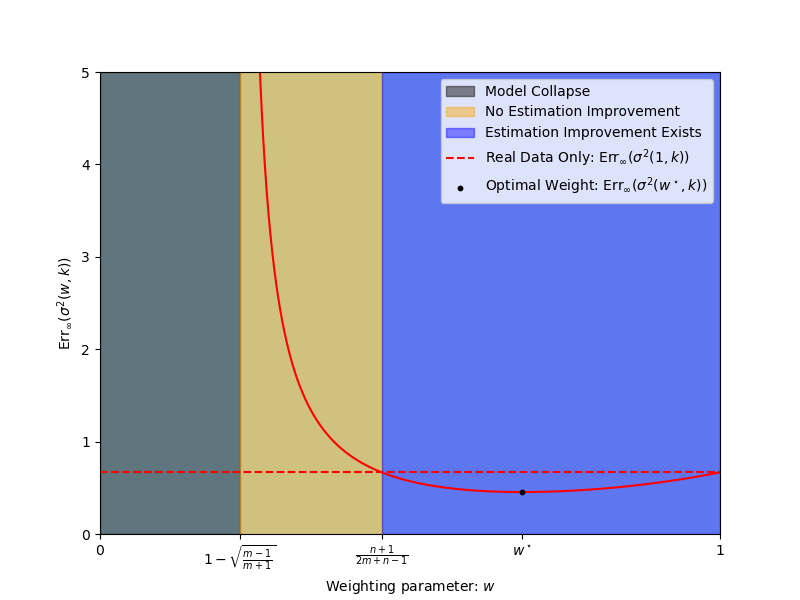
(a) Phase Transition of $\mathrm{Err}(\sigma_{\infty}^{2}(w,k))$

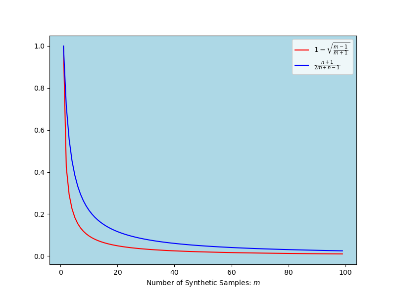
(b) Phase Vanishing of $\mathrm{Err}(\sigma_{\infty}^{2}(w,k))$

Figure 7: The left panel illustrates the quantitative behavior of $\mathrm{Err}(\sigma_{\infty}^{2}(w,k))$ with $n=m=4$ across three phases: (1) the model collapse phase, (2) the phase with no estimation improvement, and (3) the phase with estimation improvement. The right panel shows that the first two phases vanish as more synthetic samples are used for estimation with $n=4$.

An intriguing finding from Theorem 2 is the presence of a phase transition in the estimation error $\mathrm{Err}(\sigma_{\infty}^{2}(w,k))$ as shown in Figure 7. Specifically, for finite values of $m$ and $n$, the error $\mathrm{Err}(\sigma_{\infty}^{2}(w,k))$ diverges to infinity whenever $w\leq 1-\sqrt{\frac{m-1}{m+1}}$, a phenomenon we refer to as the model collapse phase. In contrast, when $w$ falls within the interval $\left(1-\sqrt{\frac{m-1}{m+1}},\frac{n+1}{2m+n-1}\right]$, the estimation error remains finite but is still worse than $\mathrm{Err}(\sigma_{\infty}^{2}(1,k))$. This indicates that incorporating synthetic data in recursive training does not outperform estimation based solely on newly emerging data. We term this region the phase of estimation without improvement. Finally, when $w>\frac{n+1}{2m+n-1}$, we obtain $\frac{\mathrm{Err}(\sigma_{\infty}^{2}(w,k))}{\mathrm{Err}(\sigma_{\infty}^{2}(1,k))}<1$, signifying the existence of estimation improvement. In this regime, optimal estimation efficiency is achieved at $w^{\star}$, as defined in Theorem 2.

Building on the analysis above, we now examine an asymptotic regime where $n=m\to\infty$. In this setting, the threshold simplifies to $w=\frac{1}{3}$, providing a clear criterion for assessing the impact of synthetic data incorporation. Specifically, synthetic data remains beneficial for estimation as long as its weight does not exceed $1-\frac{1}{3}=\frac{2}{3}$. This conclusion also holds for the mean estimation. Specifically, by Theorem 1, when $n=m$, the error ratio satisfies

$$\frac{\mathrm{Err}(\mu_{\infty}(w^{\star},k))}{\mathrm{Err}(\mu_{\infty}(1,k))}=\frac{w^{2}+(1-w)^{2}}{2w-w^{2}}<1\quad\text{if and only if}\quad\tfrac{1}{3}<w<1.$$

Hence, when $w$ exceeds $\tfrac{1}{3}$, or equivalently, the synthetic-data weight is below $\tfrac{2}{3}$, the combined estimator outperforms the estimator based solely on real data.

Corollary 2.

$\mathrm{Err}(\sigma_{\infty}^{2}(w,k))$ exhibits the following special cases

• Fully Synthetic - Model Collapse: $\lim_{w\rightarrow 0^{+}}\mathrm{Err}(\sigma_{\infty}^{2}(w,k))=\infty$,

• Real Data Only: $\mathrm{Err}(\sigma_{\infty}^{2}(1,k))=\frac{2\sigma^{4}}{n-1}$,

• Asymptotic Optimal Weight: $\mathrm{Err}\big{(}\sigma_{\infty}^{2}(w^{\star},k)\big{)}=\frac{2}{n-1}\left(\frac{\sqrt{k^{2}+4k}-k}{2}\right)\sigma^{4}+o(n^{-1})$ as $m\to\infty,n\to\infty,\frac{n}{m}\to k$, for any $k\in\mathbb{R}_{\geq 0}$,

where $w^{\star}=\frac{\sqrt{n^{2}+\left(4m-2\right)n-4m+5}-n+3}{2m+2}$ is the optimal weight as defined in Theorem 2, which converges to $\frac{\sqrt{5}-1}{2}$, the reciprocal of golden ratio, as $n=m\to\infty$.

In Corollary 2, we present several special cases of Theorem 2. As $w$ approaches zero, the estimation error $\mathrm{Err}(\sigma_{\infty}^{2}(w,k))$ diverges to infinity. However, as noted earlier, model collapse does not occur solely in the fully synthetic case. For instance, when $m=3$, the estimation error $\mathrm{Err}(\sigma_{\infty}^{2}(w,k))$ always diverges for any $w\leq 1-\sqrt{2}/2$. If estimation relies exclusively on newly emerging real data, the error is given by $\mathrm{Err}(\sigma_{\infty}^{2}(1,k))=\frac{2\sigma^{4}}{n-1}$. By using the optimal weight $w^{\star}$ defined in Theorem 2, the proposed estimator $\mathrm{Err}\big{(}\sigma_{\infty}^{2}(w^{\star},k)\big{)}$ achieves a faster convergence rate compared to estimation based solely on real data, demonstrating the utility of synthetic data.

The results of univariate Gaussian estimation are extended to the multivariate setting in Appendix A.1. Compared to the univariate case, new complexities arise due to the nontrivial analysis of correlations among the variables. In particular, while the results for mean estimation remain similar to those in the univariate case, variance estimation becomes substantially more complicated. Nevertheless, it is surprising that the multivariate case exhibits the same phase transition and, asymptotically, the same optimal weight as the univariate case.

4 Linear Regression Model

In this section, we explore the phenomenon of model collapse under the fresh data augmentation framework in linear regression. Specifically, we follow the setting in Gerstgrasser et al., (2024), where $\bm{X}=(\bm{X}_{1},\ldots,\bm{X}_{n})^{T}\in\mathbb{R}^{n\times p}$ is fixed at every step. In the initial stage, a real dataset $\mathcal{D}_{0}=\{(\bm{X}_{i},Y_{0,i})\}_{i=1}^{n}$ is generated as follows:

$$Y_{0,i}=\bm{X}_{i}^{T}\bm{\beta}+\epsilon_{0,i},\quad\text{for }i=1,\ldots,n,$$

where $\bm{\beta}$ is the true parameter, and $\epsilon_{0,i}\sim N(0,\sigma^{2})$. Subsequently, at the $t$-th step, a synthetic dataset $\mathcal{D}_{t}=\{(\bm{X}_{i},\widetilde{Y}_{t,i})\}_{i=1}^{n}$ and a new real dataset $\mathcal{D}_{t}=\{(\bm{X}_{i},Y_{t,i})\}_{i=1}^{n}$ emerge and are generated as follows:

Newly Emerging Real Data at the $$t Y_{t,i}=\bm{X}_{i}^{T}\bm{\beta}+\epsilon_{t,i},\quad\text{for }i=1,\ldots,n,$$-th Step:

Synthetic Data at the $$t \widetilde{Y}_{t,i}=\bm{X}_{i}^{T}\widehat{\bm{\beta}}_{t}(w)+\widetilde{\epsilon}_{t,i},\quad\text{for }i=1,\ldots,n,$$-th Step:

where $\widehat{\bm{\beta}}(w)$ represents the fitted regression coefficient in the $t$-th generative model and $w$ represents the weighting parameter.

The estimation scheme for $\widehat{\bm{\beta}}_{t}(w)$ follows a similar approach as before, and the overall procedure is summarized in Fresh Data Augmentation Framework 2. Specifically, we propose minimizing a weighted squared error at each step of the recursive estimation procedure. Specifically, at the $t$-th step, $\widehat{\bm{\beta}}_{t}(w)$ is obtained by solving the following optimization task:

$$\widehat{\bm{\beta}}_{t}(w)=\arg\min_{\bm{\beta}}\left\{w\|\bm{Y}_{t}-\bm{X}\bm{\beta}\|_{2}^{2}+(1-w)\|\widetilde{\bm{Y}}_{t}-\bm{X}\bm{\beta}\|_{2}^{2}\right\},$$ (4)

where $\bm{Y}_{t}=(Y_{t,1},\ldots,Y_{t,n})^{T}$ and $\widetilde{\bm{Y}}_{t}=(\widetilde{Y}_{t,1},\ldots,\widetilde{Y}_{t,n})^{T}$. The weighting parameter $w$ determines the emphasis placed on the real data emerging at $t$-th step, controlling the balance between real and synthetic data in the optimization process.

Algorithm 2 - Linear Regression with Fixed Design

 Initialization: Compute the initial estimate of $\widehat{\bm{\beta}}_{0}(w)$ based on the dataset $\mathcal{D}_{0}=\{(\bm{X}_{i},Y_{0,i})\}_{i=1}^{n}$, where $Y_{0,i}=\bm{X}_{i}\bm{\beta}+\epsilon_{0,i}$ and $\epsilon_{0,i}\sim N(0,\sigma^{2})$:

$$\widehat{\bm{\beta}}_{0}(w)=(\bm{X}^{\top}\bm{X})^{-1}\bm{X}^{\top}\bm{Y}_{0}.$$ (5)

 for $t=1,2,\ldots,T$ do

  1. Data Collection: Collect two datasets:

• A new synthetic dataset $\widetilde{\mathcal{D}}_{t}=\{(\bm{X}_{i},\widetilde{Y}_{t,i})\}_{i=1}^{n}$, where $\widetilde{Y}_{t,i}=\bm{X}_{i}^{T}\widehat{\bm{\beta}}_{t-1}(w)+\widetilde{\epsilon}_{t,i}$ and $\widetilde{\epsilon}_{t,i}\sim N(0,\sigma^{2})$.

• A new real dataset $\mathcal{D}_{t}=\{(\bm{X}_{i},Y_{t,i})\}_{i=1}^{n}$, where $Y_{t,i}=\bm{X}_{i}^{T}\bm{\beta}+\epsilon_{t,i}$ and $\epsilon_{t,i}\sim N(0,\sigma^{2})$.

  2. Parameter Estimation: Compute the regression coefficients at the $t$-th step by the following closed-form solution:

$$\widehat{\bm{\beta}}_{t}(w)=(\bm{X}^{T}\bm{X})^{-1}\bm{X}^{T}\left(w\bm{Y}_{t}+(1-w)\widetilde{\bm{Y}}_{t}\right).$$

 end for

 return  $\widehat{\bm{\beta}}_{T}(w)$.

Similarly, we examine the testing performance of the resulting estimator $\widehat{\bm{\beta}}_{T}(w)$. Following the framework of Gerstgrasser et al., (2024), we assess the quality of $\widehat{\bm{\beta}}_{T}(w)$ using the metric:

$$\mathrm{Err}(\widehat{\bm{\beta}}_{T}(w))=\mathbb{E}\left[\|\widehat{\bm{\beta}}_{T}(w)-\bm{\beta}\|_{2}^{2}\right],$$

where the expectation is taken over the design matrix $\bm{X}$ and the noise terms $\bm{\epsilon}_{t}=(\epsilon_{t,1},\ldots,\epsilon_{t,n})$ and $\widetilde{\bm{\epsilon}}_{t}=(\widetilde{\epsilon}_{t,1},\ldots,\widetilde{\epsilon}_{t,n})$ for $t\geq 1$.

Similar to the previous results, we are interested in the behavior of $\mathrm{Err}_{T}(w)$ as $T$ approaches infinity. Under the normality assumption of $\bm{\epsilon}_{t}$ and $\widetilde{\bm{\epsilon}}_{t}$, the expression for $\mathrm{Err}(\widehat{\bm{\beta}}_{T}(w))$ can be readily derived using the results from Theorem 4 in Appendix A.1. A key distinction in the Fresh Data Augmentation Framework 2, compared to the previous results, is the assumption that $n=m$. This assumption stems from the fact that $\bm{X}$ remains fixed throughout the recursive training process, with only the labels being synthetic.

Theorem 3.

For any $n\geq 2$, it holds that

$$\mathrm{Err}(\widehat{\bm{\beta}}_{\infty}(w))\triangleq\lim_{T\to\infty}\mathrm{Err}(\widehat{\bm{\beta}}_{T}(w))=\sigma^{2}\frac{2w^{2}-2w+1}{2w-w^{2}}\mathbb{E}_{\bm{X}}\left[\mathrm{tr}\left\{(\bm{X^{T}X})^{-1}\right\}\right],$$ (6)

and the optimal $w^{\star}=\frac{\sqrt{5}-1}{2}$, which is the reciprocal of the golden ratio. The estimation error improves compared to using only real data, i.e. $\mathrm{Err}(\widehat{\bm{\beta}}_{\infty}(w))<\mathrm{Err}(\widehat{\bm{\beta}}_{\infty}(1))$, if and only if $w\in(\frac{1}{3},1)$.

In Theorem 3, we analyze the limiting estimation error $\mathrm{Err}(\widehat{\bm{\beta}}_{\infty}(w))$ in the context of linear regression. Specifically, we derive the exact form of $\mathrm{Err}(\widehat{\bm{\beta}}_{\infty}(w))$ in (6), which allows us to identify several interesting scenarios. Notably, to achieves the fastest convergence rate, the optimal weight $w^{\star}$ for our proposed estimator corresponds to the reciprocal of the golden ratio. Additionally, our result also aligns with existing results regarding the model collapse in the context of linear regression (Gerstgrasser et al.,, 2024). Specifically, by letting $w$ approach zero, the estimation error $\mathrm{Err}(\widehat{\bm{\beta}}_{\infty}(w))$ diverges to infinity, leading to model collapse.

5 Discussion on the Optimal Ratio of Real to Synthetic Data

In this section, we discuss the selection of the mixing proportion between real and synthetic data from a practical perspective. Through Theorems 1-3, we observe that, within the fresh data augmentation framework, different generative modeling scenarios exhibit varying estimation errors in the finite sample setting. However, their asymptotic estimation errors conform to a unified mathematical form:

$$\text{Estimation Error}\propto\frac{C(w,k)}{n}+o\left(\frac{1}{n}\right),$$ (7)

where $C(w,k)=\frac{w^{2}+(1-w)^{2}k}{2w-w^{2}}$ and $k=n/m$. For a fixed $k$, $C(w,k)$ is minimized at $w^{\star}=\frac{\sqrt{k^{2}+4k}-k}{2}$, and the corresponding minimum value is

$$C(w^{\star},k)=\frac{\sqrt{k^{2}+4k}-k}{2}=w^{\star}.$$ (8)

Interestingly, the minimizer is also a fixed point of the function.

Synthetic Data Improves Estimation. The result in (8) offers practical insights for selecting the weight $w$ and the proportion $k$. If the amount of real data $n$ is fixed, we observe that choosing the optimal weight $w^{\star}$ results in a smaller value of $C(w,k)$. Note that $C(w^{\star},k)=\frac{\sqrt{k^{2}+4k}-k}{2}$ will decrease as $k$ decreases. This implies that, if the number of real data points per iteration is fixed, increasing the number of synthetic data points improves performance during iterative training. In fact, through further verification, we can prove that this result holds not only when $T\to\infty$, but also for any finite number of iterations, and even for an arbitrary fixed weight $w$. Intuitively, a larger amount of synthetic data ensures that the information inherited from previous iterations remains cleaner, leading to better overall performance.

Cost of Using Synthetic Data. Even though utilizing more synthetic data can always improve estimation efficiency in our setting, in practice, obtaining a large amount of synthetic data may incur some cost. Therefore, one must consider the tradeoff between cost and estimation error. Consider a specific scenario in which the total budget per iteration constrains the combined amount of real and synthetic data. Specifically, we assume that acquiring one unit of synthetic data costs a fraction $r$ (where $0<r<1$) of the cost of collecting one unit of real data. This assumption implies that obtaining a synthetic data point is cheaper than obtaining a real data point for training. Under this budgeted setting, the total data per iteration must satisfy $n+rm=S$, where $n$ and $m$ denote the size of real and synthetic data, respectively, and $S$ represents the fixed total budget allocated for data collection in each iteration. Then we can rewrite the estimation error in (7) as follows

$$\text{Estimation Error}\propto\underbrace{\frac{1}{S}\frac{k+r}{k}\frac{\sqrt{k^{2}+4k}-k}{2}}_{\text{Dominant Term}}+o(S^{-1}).$$ (9)

Here, it can be proved that the dominant term is minimized at $k=\frac{r^{\frac{3}{2}}+r}{1-r}$. A detailed derivation is provided in Appendix A.3.

The result in (9) indicates that, given a fixed budget $S$ each step and the relative cost $r$ of synthetic data compared to real data, the optimal data ratio of real to synthetic data should be $k=\frac{r^{\frac{3}{2}}+r}{1-r}$. From this result, we can derive several special cases that provide insights into how synthetic data should be used in a cost-effective way:

• When $r=\left(\frac{\sqrt{5}-1}{2}\right)^{2}$ (the squared inverse golden ratio): The optimal proportion simplifies to $k=\frac{n}{m}=1$, meaning real and synthetic data should be used in equal proportions. Interestingly, at this point, the optimal weight $w^{\star}$ aligns with the reciprocal of the golden ratio, as discussed earlier.

• When $r=0$ (i.e., synthetic data is free): The optimal strategy is to use as much synthetic data as possible, as increasing its quantity improves performance without additional cost. This suggests that in cases where generating synthetic data incurs no expense, it should be leveraged extensively to enhance model training.

• As $r\to 1$ (i.e., the cost of synthetic data approaches that of real data): The optimal ratio $k\to\infty$, meaning synthetic data becomes less cost-effective. In this case, relying on synthetic data is no longer advantageous in terms of budgeting, and real data should be prioritized.

6 Experiments

In this section, we present a series of simulations and a real-world application to validate our theoretical findings. Our objectives are three-fold. First, we demonstrate the existence of an optimal weight for weighted training, particularly when real and synthetic data are present in equal amounts. Second, we illustrate that the fresh data augmentation framework improves estimation efficiency compared to other frameworks. Third, we highlight the phase transition phenomenon in the usefulness of synthetic data, which depends on variations in synthetic sample size and weighting.

6.1 Simulations

Scenario 1 (Model Collapse in Fully Synthetic Case): In this scenario, we aim to validate our results on Gaussian distribution estimation and linear regression. For the experimental setup, we consider the following configurations: (1) In Gaussian estimation, the parameters are set as $\bm{\mu}=(0,0,0,0)$ and $\bm{\Sigma}=\bm{I}_{4}$. (2) In linear regression, we use $\bm{\beta}=(1,1,1,1)$, with noise modeled by a standard normal distribution. The sample size is fixed at 100 for all experiments, with each experiment involving $1,000$ recursive estimation steps. To estimate the values of $\mathrm{Err}(\bm{\mu}_{t}(w,k))$, $\mathrm{Err}(\bm{\Sigma}_{t}(w,k))$, and$\mathrm{Err}(\widehat{\bm{\beta}}_{t}(w))$ for $t\in\{1,2,\ldots,10^{3}\}$, each experimental setup is replicated $1,000$ times.

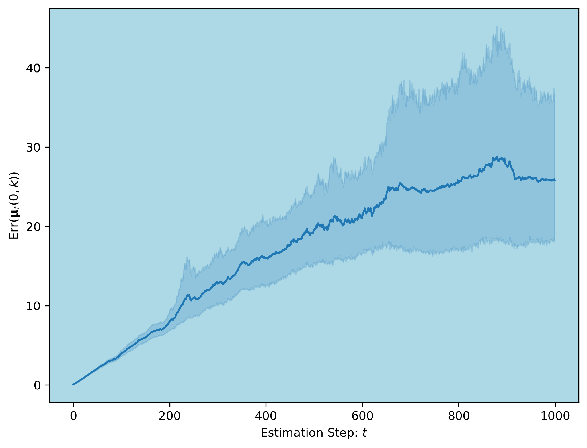
(a) Gaussian Mean

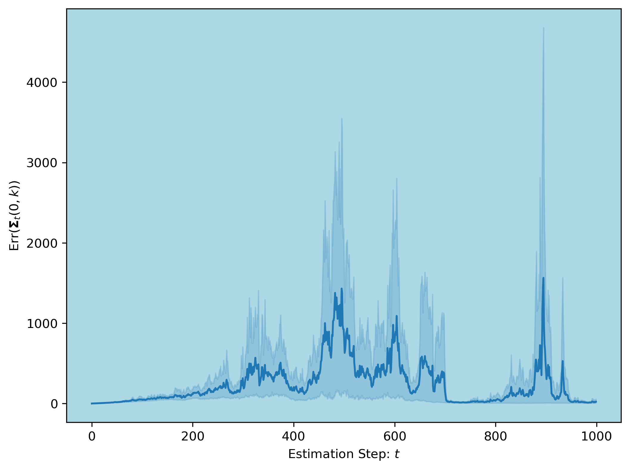
(b) Gaussian Variance

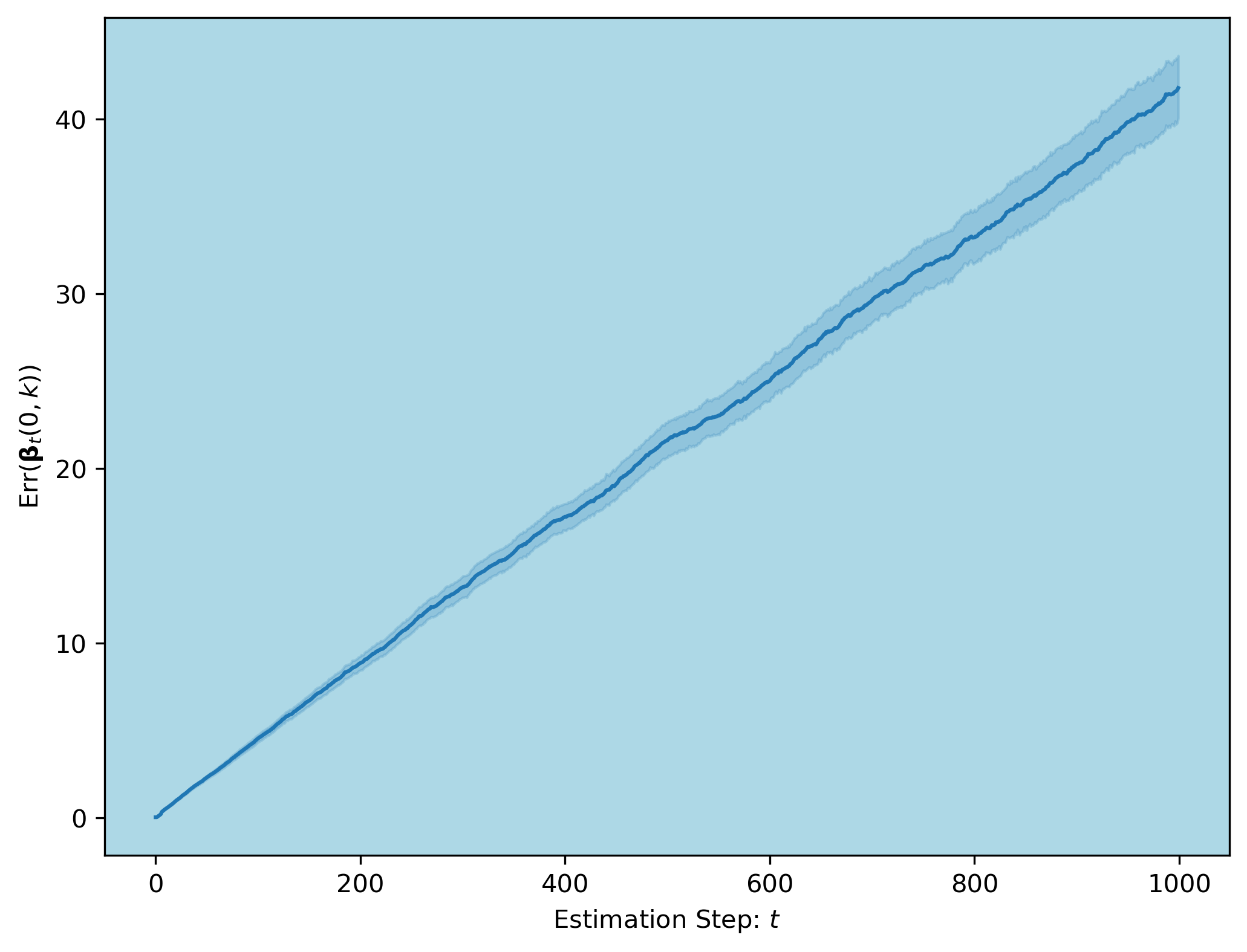
(c) Linear Regression

Figure 8: The averaged values of estimation errors $\mathrm{Err}(\bm{\mu}_{t}(w,k))$, $\mathrm{Err}(\bm{\Sigma}_{t}(w,k))$, and $\mathrm{Err}(\widehat{\bm{\beta}}_{t}(w))$ over $1,000$ replications during the first $1,000$ steps in the fully synthetic case $(w=0)$ are reported for Scenario I (Fully Synthetic Case).

Figure 8 presents the averaged estimation errors in Gaussian estimation and linear regression, estimated over $1,000$ replications for each $t\in\{1,2,\ldots,10^{3}\}$. For the multivariate Gaussian distribution, $\mathrm{Err}(\bm{\mu}_{t}(0,k))$ increases gradually with $t$, and the 95% confidence intervals for $\|\bm{\mu}_{t}(0,k)-\bm{\mu}\|_{2}^{2}$ widen as $t$ grows. Consistently, as $t$ approaches infinity, $\mathrm{Err}(\bm{\mu}_{t}(w,k))$ diverges to infinity, corroborating our result in Corollary 3. Moreover, for covariance matrix estimation, the estimation error $\mathrm{Err}(\bm{\Sigma}_{t}(w,k))$ diverges more significantly as $t$ increases, indicating that the estimation of the true covariance matrix $\bm{\Sigma}$ becomes highly inaccurate. This result also aligns with Corollary 4. For linear regression, $\mathrm{Err}(\widehat{\bm{\beta}}_{t}(w))$ increases linearly with $t$ when $w=0$. As expected, $\mathrm{Err}(\widehat{\bm{\beta}}_{\infty}(w))$ becomes infinite, in line with Theorem 3.

Scenario 2 (Golden Ratio Verification): In this scenario, we aim to validate our theoretical findings, which suggest that when $n=m$, the optimal proportion of synthetic data corresponds to the reciprocal of the golden ratio. To achieve this, we adopt the same experimental setup for simulated data generation as outlined in Scenario 1, with $w\in\{0.2+0.02\times i\mid i\in[30]\}$ and $(n,T,k)=(100,10^{3},1)$. To estimate the limiting estimation errors, we use the average of the last 100 estimation errors as an approximation. For instance, in Gaussian mean estimation, we approximate $\mathrm{Err}(\bm{\mu}_{\infty}(w,k))$ using

$$\mathrm{Err}(\bm{\mu}_{\infty}(w,k))\approx\frac{1}{100}\sum_{t=900}^{1,000}\mathrm{Err}(\bm{\mu}_{t}(w,k)).$$ (10)

Each case is repeated 10,000 times, and the average estimated limiting errors, along with their 95% confidence intervals, are reported in Figure 9.

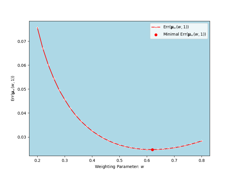
(a) Gaussian Mean

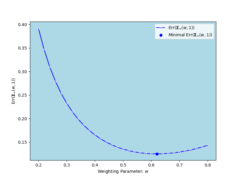
(b) Gaussian Variance

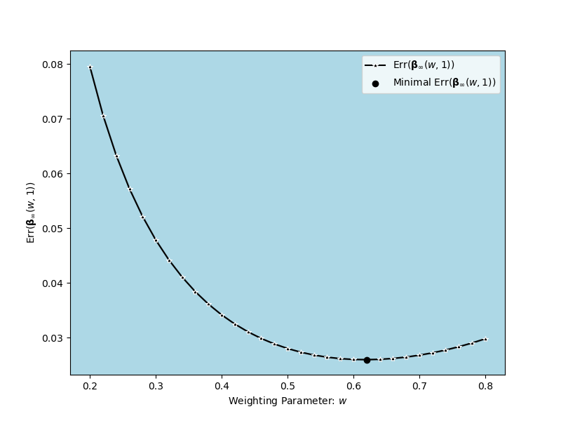
(c) Linear Regression

Figure 9: The averaged values of estimation errors under different values of $w$ with $(n,T,k)=(100,10^{3},1)$ over 10,000 replications. The minimum values of estimated $\mathrm{Err}(\bm{\mu}_{\infty}(w,k))$, $\mathrm{Err}(\bm{\Sigma}_{\infty}^{2}(w,k))$, and $\mathrm{Err}(\widehat{\bm{\beta}}_{\infty}(w))$ are highlighted

The results in Figure 9 align with our theoretical findings. Specifically, when $n=m$ ($k=1$), the optimal weighting parameter that minimizes all estimation errors is approximately 0.62, as shown in Figure 9. Notably, this value is the closest, within the experimental range $w\in\{0.2+0.02\times i\mid i\in[30]\}$, to the reciprocal of the golden ratio, i.e., $\frac{\sqrt{5}-1}{2}$.

Scenario 3 (Synthetic Data Helps Reduce Error using Optimal Weighting): In this scenario, we aim to demonstrate that synthetic data can effectively reduce estimation errors using the optimal mixing proportion within the fresh data augmentation framework. To illustrate this, we consider Gaussian distribution estimation and fix $(n,T)=(100,10^{3})$, following the same experimental setup for simulated data generation as described in Scenario 1. We vary the number of synthetic data points per round, considering $m\in\{100\times i\mid i\in[10]\}$.

For our method, we set $w$ as the optimal weight, given by $w^{\star}=\frac{\sqrt{k^{2}+4k}-k}{2}$, where $k=n/m$. For comparison, we also report the estimation errors of the data accumulation framework (Figure 2) and the data augmentation framework (Figure 3). As a baseline, we include the estimation error of the estimator based solely on first-round real data, $\mathcal{D}_{0}$.

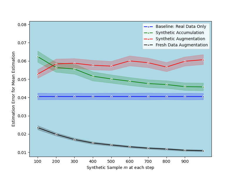
(a) Gaussian Mean Estimation

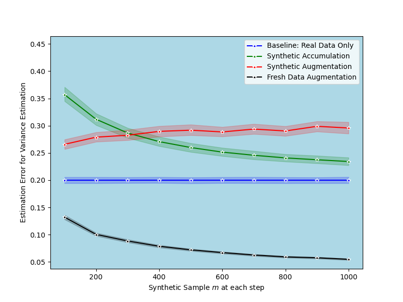
(b) Gaussian Variance Matrix Estimation

Figure 10: The averaged estimation errors for estimating the Gaussian mean and covariance matrix under the synthetic accumulation, synthetic augmentation, and fresh data augmentation frameworks, with varying synthetic sample sizes $m\in\{100,200,\dots,10^{3}\}$ and $n=100$.

Figure 10 shows that, under the synthetic accumulation and synthetic augmentation frameworks, the estimation errors for the Gaussian mean and covariance matrix are higher than those obtained using only real data. This result suggests that synthetic data in these two frameworks degrades estimation performance and conveys little useful information for learning the true distribution. In contrast, under the fresh data augmentation framework, synthetic data effectively reduces estimation errors compared to the real data-only case, regardless of synthetic sample size. This indicates that synthetic data provides useful information for learning the true distribution. As expected, as $m$ increases, estimation errors decrease. This result aligns with our theoretical results in Theorems 4 and 5.

Scenario 4 (Phase Transition Phenomenon Induced by Weighting):In this scenario, we aim to demonstrate the existence of a phase transition phenomenon in the helpfulness of synthetic data, which depends on the value of $w$, as illustrated in Figure 7. To illustrate this, we consider the case where $n=m=100$ and $T=1,000$. As demonstrated by Theorems 1 and 2, synthetic data contributes to reducing estimation errors for both the mean and the variance matrix in a Gaussian distribution when $w>1/3$, which indicates that the weight assigned to real data in the weighted training scheme should be higher than $1/3$. To this end, we consider $w\in\{0.1+0.01\times i\mid i\in[90]\}$ and replicate each experimental setting 1,000 times. The corresponding limiting errors are estimated via (10).

(a) Mean Estimation: $p=1$

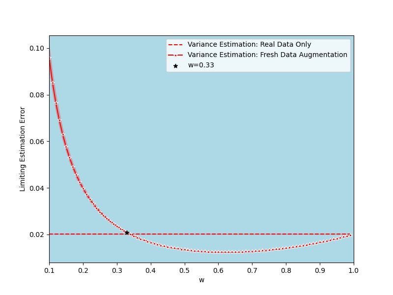
(b) Variance Estimation: $p=1$

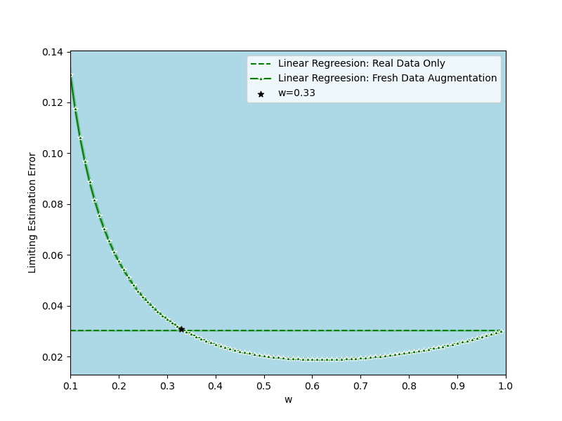
(c) Linear Regression: $p=1$

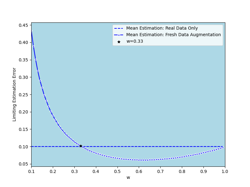
(d) Mean Estimation: $p=10$

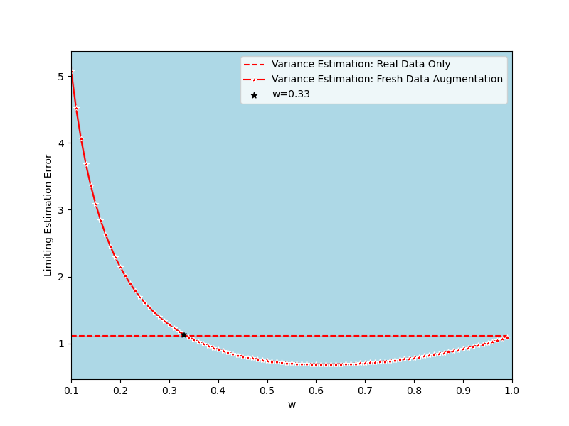
(e) Variance Estimation: $p=10$

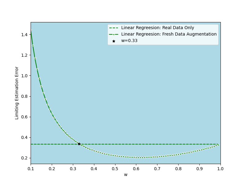
(f) Linear Regression: $p=10$

Figure 11: The averaged limiting estimation errors for Gaussian mean and variance estimation in cases $p=1$ (Top) and $p=10$ (Bottom) under varying values of $w$.

6.2 Real Application-Adult Dataset

In this section, we use the Adult dataset (Becker and Kohavi,, 1996) to empirically validate our theoretical findings on model collapse. The dataset consists of 48,842 instances, each with 14 features used to predict whether an individual’s annual income exceeds $50K$. These features include continuous variables such as capital-gain, age, and hours-per-week, which, although rounded to integers, maintain their continuous nature. Additionally, the dataset contains categorical variables, including education level, race, and others.

In this application, we pursue two main objectives. First, we demonstrate that the fresh data augmentation framework achieves superior estimation efficiency compared to other framework. Second, we seek to validate our theoretical findings on the optimal choice of weighting parameters. Our analysis primarily focuses on estimating the means and variances of age and hours-per-week.

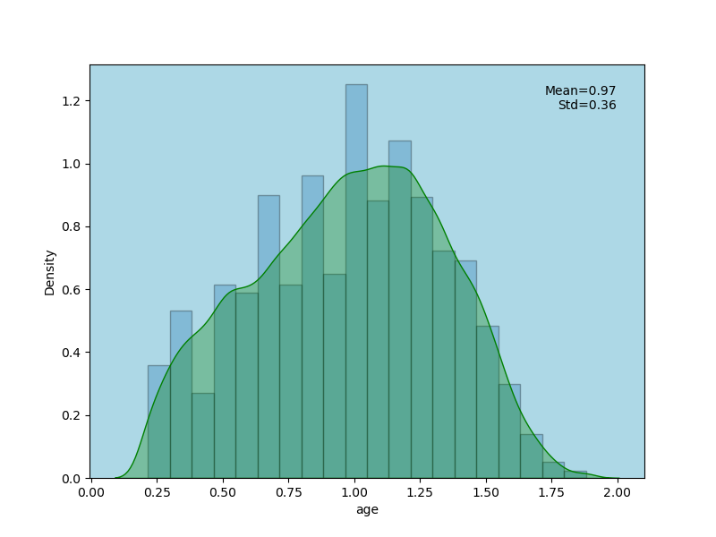
(a) Logarithm of Age

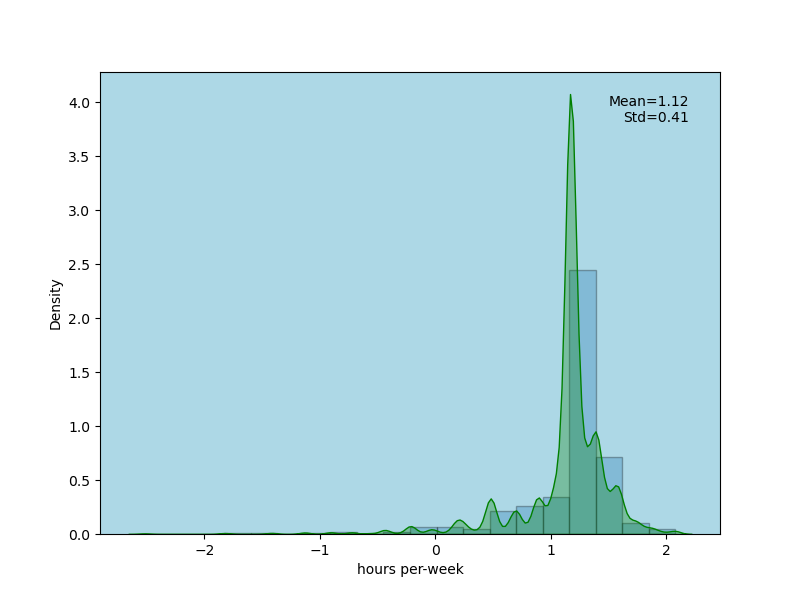
(b) Logarithm of Hours Per-week

Figure 12: The empirical distributions and densities of the logarithms of age (left) and weekly working hours (right).

We begin by applying a log transformation to both variables and visualizing their histograms along with their density estimates in Figure 12. This transformation makes the distributions of both variables more closely resemble normal distributions. In the first experiment, we consider the same experimental setting as in Scenario 3, with a fixed sample size of $n=200$ and a varying synthetic sample size each round, given by $m\in\{100\times i\mid i\in[10]\}$. For our framework, we utilize the optimal weight, defined as $w^{\star}=\frac{\sqrt{k^{2}+4k}-k}{2}$, where $k=n/m$. In the second experiment, we aim to demonstrate that synthetic data can help reduce estimation errors under appropriate choices of weights. Specifically, we consider $n=m=200$ and vary the weights as $w\in\{0.1+0.01\times i\mid i\in[90]\}$. Each case is replicated 1,000 times and the averaged limiting estimation errors of all cases are reported in Figure 13.

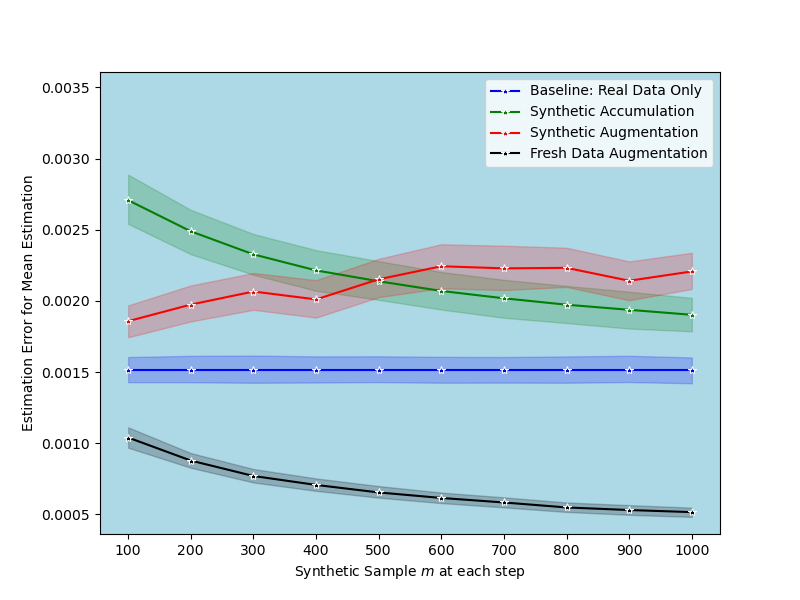
(a) Varying $m$: Mean Estimation

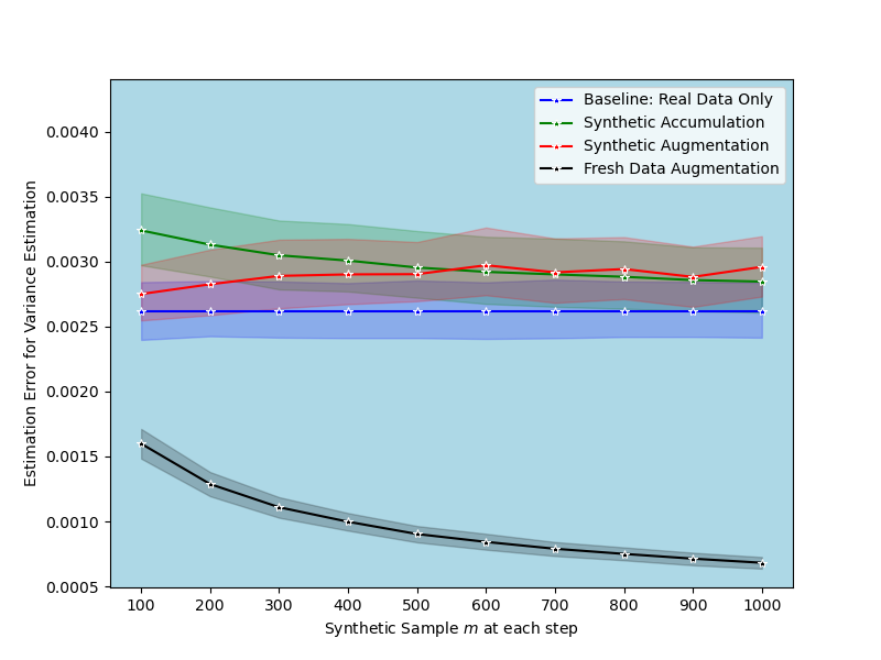
(b) Varying $m$: Variance Estimation

(c) Varying $w$: Mean Estimation

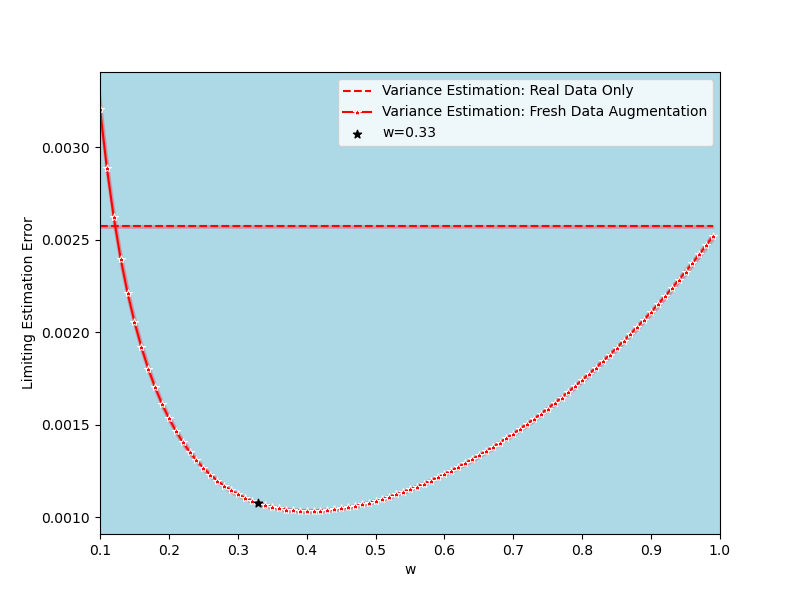
(d) Varying $m$: Variance Estimation

Figure 13: The averaged limiting estimation errors over 1,000 replications for comparing different frameworks (Top) and varying weight $w$ under the proposed framework (Bottom).

The experimental results presented in Figure 13 convey several key messages. First, compared to other frameworks, the fresh data augmentation framework highlights the utility of synthetic data in reducing estimation errors. Notably, as the size of the synthetic dataset increases, the estimation of both the mean and variance matrix improves beyond what is achievable using real data alone. Second, in mean estimation, we observe that when the real and synthetic datasets have equal sample sizes in each round, the optimal weight for the mean estimator aligns with the reciporal of the golden ratio. However, this phenomenon does not extend to variance estimation. The underlying discrepancy primarily to model misspecification. In other words, the real data is not normally distributed. In our theoretical results, we assume a normal distribution for the generative model, which provides an unbiased estimate of the second moment of the true distribution. This property leads to the emergence of the golden ratio in mean estimation. However, the generative model fails to accurately capture the fourth moment of the real data, preventing a similar result for variance estimation. The key message is that to achieve a golden-ratio outcome for a general generative model, the model must be able to approximate the real distribution. Since this condition is not met in variance estimation when applied to real data analysis, the golden ratio does not emerge as the optimal weight.

7 Discussion and Future Work

In this paper, we investigate the phenomenon of model collapse within a data augmentation framework, where each training round incorporates both newly collected real data and synthetic data generated by the model from the previous iteration. Our theoretical analysis considers a fixed mixing proportion and weighting scheme throughout the recursive training process, examining how these factors influence the final model’s performance. Notably, in the setting where the ratio of synthetic to real data is 1:1, we uncover a striking connection to the golden ratio: in the large-sample regime, the optimal training weight for real data is given by the reciprocal of the golden ratio. These findings underscore a fundamental trade-off between leveraging synthetic data for efficiency gains and maintaining model performance across multiple iterations.

Despite these insights, several open questions remain. A key assumption in our analysis is that the weights assigned to real and synthetic data remain fixed throughout training. A natural extension is to explore an adaptive weighting scheme, where these weights evolve dynamically at each iteration. Investigating such adaptive strategies could provide deeper insights into optimal training dynamics and further clarify the role of synthetic data in long-term learning stability. Another critical direction is the statistical properties of our estimation method. In this paper, we establish that our approach yields the Best Linear Unbiased Estimator (BLUE) under the assumption that the estimation scheme remains fixed in each round. However, an important open question is whether it remains the best unbiased estimator in a more general sense. Conventional techniques, such as the Cramér-Rao Lower Bound, do not directly apply to iterative estimation procedures, making it challenging to derive general optimality results. Developing novel theoretical tools to analyze model collapse from an information-theoretic perspective will offer deeper insights into the statistical behavior of iterative learning processes.

Appendix A.1 Additional Results on Multivariate Gaussian Estimation

In this part, we extend our results from Section 3 to a multivariate setting. Specifically, we assume the real data distribution follows $N(\bm{\mu},\bm{\Sigma})$, where $\bm{\mu}\in\mathbb{R}^{p}$ is the mean vector and $\bm{\Sigma}\in\mathbb{R}^{p\times p}$ is the covariance matrix. The goal of recursive estimation is to estimate $\bm{\mu}$ and $\bm{\Sigma}$ simultaneously. Compared to the univariate case, new complexities arise due to the nontrivial analysis in the correlation among variables.

Let $\mathcal{D}_{t}=\{\bm{x}_{t,i}\}_{i=1}^{n}$ denote the real dataset collected at the $t$-th training step, and let $\widetilde{\mathcal{D}}_{t}=\{\widetilde{\bm{x}}_{t,i}\}_{i=1}^{n}$ represent the synthetic dataset generated at the $(t-1)$-th generation step. The estimation scheme follows a similar approach to the univariate case, and the overall procedure is summarized in Fresh Data Augmentation Case 3. Specifically, we consider the following weighted estimation scheme at the $t$-th training step:

Mean Estimation: $$\bm{\mu}_{t}(w,k)=\mathop{\mathrm{argmin}}_{\bm{\mu}\in\mathbb{R}^{p}}\frac{w}{n}\sum_{i=1}^{n}\|\bm{\mu}-\bm{x}_{t,i}\|_{2}^{2}+\frac{1-w}{m}\sum_{i=1}^{m}\|\bm{\mu}-\widetilde{\bm{x}}_{t,i}\|_{2}^{2},$$ (1)

Variance Estimation: $$\bm{\Sigma}_{t}(w,k)=\mathop{\mathrm{argmin}}_{\bm{\Sigma}\in\mathbb{R}^{p\times p}}w\|\bm{\Sigma}-\widehat{\bm{S}}_{t}\|_{F}^{2}+(1-w)\|\bm{\Sigma}-\widetilde{\bm{S}}_{t}\|_{F}^{2},$$ (2)

where $\widehat{\bm{S}}_{t}=\frac{1}{n-1}\sum_{i=1}^{n}(\bm{x}_{t,i}-\widehat{\bm{\mu}}_{t})(\bm{x}_{t,i}-\widehat{\bm{\mu}}_{t})^{T}$ and $\widetilde{\bm{S}}_{t}=\frac{1}{m-1}\sum_{i=1}^{m}(\widetilde{\bm{x}}_{t,i}-\widetilde{\bm{\mu}}_{t})(\widetilde{\bm{x}}_{t,i}-\widetilde{\bm{\mu}}_{t})^{T}$ with with $\widehat{\bm{\mu}}_{t}=\frac{1}{n}\sum_{i=1}^{n}\bm{x}_{t,i}$ and $\widetilde{\bm{\mu}}_{t}=\frac{1}{m}\sum_{i=1}^{m}\widetilde{\bm{x}}_{t,i}$.

Similarly, we define the following metrics to analyze the quantitative behavior of $\bm{\mu}_{t}(w,k)$ and $\bm{\Sigma}_{t}(w,k)$ especially when $t$ increases to infinity:

$$\text{Err}(\bm{\mu}_{t}(w,k))=\mathbb{E}\big{[}\|\bm{\mu}_{t}(w,k)-\bm{\mu}\|_{2}^{2}\big{]}\mbox{ and }\text{Err}(\bm{\Sigma}_{t}(w,k))=\mathbb{E}\big{[}\|\bm{\Sigma}_{t}(w,k)-\bm{\Sigma}\|_{F}^{2}\big{]},$$

where $\|\cdot\|_{2}$ is the $l_{2}$-norm and $\|\cdot\|_{F}$ is the Frobenius norm. Here, $\text{Err}(\bm{\mu}_{t}(w,k))$ and $\text{Err}(\bm{\Sigma}_{t}(w,k))$ quantify the estimation errors of $\bm{\mu}_{t}(w,k)$ and $\bm{\Sigma}_{t}(w,k)$, respectively. The expectation is taken with respect to the randomness inherent in all real and synthetic datasets generated during the first $t$ steps.

Algorithm 3 - Multivariate Gaussian Estimation

 Initialization: Compute $\bm{\mu}_{0}=\frac{1}{n}\sum_{i=1}^{n}\bm{x}_{0,i}$ and $\bm{\Sigma}_{0}=\frac{1}{n-1}\sum_{i=1}^{n}(\bm{x}_{0,i}-\bm{\mu}_{0})(\bm{x}_{0,i}-\bm{\mu}_{0})^{T}$ based on $\mathcal{D}_{0}=\{\bm{x}_{0,i}\}_{i=1}^{n}$ from $N(\bm{\mu},\bm{\Sigma})$;

 for $t=1,2,\ldots,T$ do

  1. Data Collection: Sample $\widetilde{\mathcal{D}}_{t}=\{\widetilde{\bm{x}}_{t,i}\}_{i=1}^{m}$ from $N(\bm{\mu}_{t-1},\bm{\Sigma}_{t-1})$ and collect a new real dataset $\mathcal{D}_{t}=\{\bm{x}_{t,i}\}_{i=1}^{n}$ from $N(\bm{\mu},\bm{\Sigma})$;

  2. Mean Estimation: Compute the mean of the Gaussian distribution at the $t$-th training step:

$$\bm{\mu}_{t}(w,k)=w\widehat{\bm{\mu}}_{t}+(1-w)\widetilde{\bm{\mu}}_{t},$$ (3)

where $\widehat{\bm{\mu}}_{t}=\frac{1}{n}\sum_{i=1}^{n}\bm{x}_{t,i}$, $\widetilde{\bm{\mu}}_{t}=\frac{1}{m}\sum_{i=1}^{m}\widetilde{\bm{x}}_{t,i}$, and $k=n/m$.

  3. Covariance Estimation: Compute the covariance of the Gaussian distribution at the $t$-th training step:

$$\bm{\Sigma}_{t}(w,k)=w\widehat{\bm{S}}_{t}+(1-w)\widetilde{\bm{S}}_{t}.,$$ (4)

where $\widehat{\bm{S}}_{t}=\frac{1}{n-1}\sum_{i=1}^{n}(\bm{x}_{t,i}-\widehat{\bm{\mu}}_{t})(\bm{x}_{t,i}-\widehat{\bm{\mu}}_{t})^{T}$ and $\widetilde{\bm{S}}_{t}=\frac{1}{m-1}\sum_{i=1}^{m}(\widetilde{\bm{x}}_{t,i}-\widetilde{\bm{\mu}}_{t})(\widetilde{\bm{x}}_{t,i}-\widetilde{\bm{\mu}}_{t})^{T}$.

 end for

 return  $\bm{\mu}_{T}(w,k)$ and $\bm{\Sigma}_{T}(w,k)$.

The central problem is analyzing the behavior of $\bm{\mu}_{t}(w,k)$ and $\bm{\Sigma}_{t}(w,k)$ as $t$ approaches infinity. Therefore, we also consider the following metrics for the case where $t=\infty$:

$$\mathrm{Err}(\bm{\mu}_{\infty}(w,k))\triangleq\lim_{t\rightarrow\infty}\mathrm{Err}\left(\bm{\mu}_{t}(w,k)\right)\mbox{ and }\mathrm{Err}(\bm{\Sigma}_{\infty}(w,k))\triangleq\lim_{t\rightarrow\infty}\mathrm{Err}\left(\bm{\Sigma}_{t}(w,k)\right).$$

In the following, we present the theoretical results on the quantitative behavior of $\mathrm{Err}(\bm{\mu}_{\infty}(w,k))$ and $\mathrm{Err}(\bm{\Sigma}_{\infty}(w,k))$ in a finite-sample setting, aiming to elucidate the impact of $w$ and $k$. Particularly, we show that while the analysis of the mean estimation closely parallels the univariate case, the analysis for variance matrix estimation introduces new complexities. Specifically, the potential correlations among variables of a multivariate normal distribution, cause the variance estimation errors across different time points to no longer follow a straightforward iterative relationship, in contrast with the one-dimensional case. Despite these technical hurdles, we find that $\mathrm{Err}(\bm{\Sigma}_{\infty}(w,k))$ can be succinctly characterized by two key quantities: $\mathrm{tr}(\mathbf{\Sigma}^{2})$ and $\left[\mathrm{tr}(\mathbf{\Sigma})\right]^{2}$, as these two terms, especially $\left[\mathrm{tr}(\mathbf{\Sigma})\right]^{2}$, can increase with dimensionality, further highlighting the necessity of appropriately choosing $w$ to reduce error.

Theorem 4.

For any $w\in(0,1]$ and $n,m\geq 1$ with $k=\frac{n}{m}$. It holds that

$$\mathrm{Err}(\bm{\mu}_{\infty}(w,k))=\lim_{t\rightarrow\infty}\mathrm{Err}(\bm{\mu}_{t}(w,k))=\frac{C(w,k)\mathrm{tr}(\bm{\Sigma})}{n},$$

where $C(w,k)=\frac{w^{2}+(1-w)^{2}k}{2w-w^{2}}$ and $\mathrm{tr}(\cdot)$ is the trace of a matrix. Using the optimal weight $w^{\star}=\frac{\sqrt{k^{2}+4k}-k}{2}$, the estimation improvement for estimating $\bm{\mu}$ is given by

$$\frac{\mathrm{Err}(\bm{\mu}_{\infty}(w^{\star},k))}{\mathrm{Err}(\bm{\mu}_{\infty}(1,k))}=w^{\star}=\frac{\sqrt{k^{2}+4k}-k}{2}<1.$$

In Theorem 4, we derive the exact expression for $\mathrm{Err}(\bm{\mu}_{\infty}(w,k))$ under different values of the weighting parameter $w$ and the mixing ratio $k$. Notably, the result in Theorem 4 simplifies to that in Theorem 1 when the data is one-dimensional. Thus, Theorem 4 can be regarded as the multivariate extension of Theorem 1.

Theorem 4 shows that $\mathrm{Err}(\bm{\mu}_{\infty}(w,k))=\frac{C(w,k)\,\mathrm{tr}(\bm{\Sigma})}{n}$ for any values of $(n,m,w)$, where $C(w,k)$ is the same as in Theorem 1. Consequently, we draw the same conclusions as in Theorem 1 regarding the choice of the optimal weight and the improvement in estimation compared to the estimator based solely on newly emerging real data. For any values of $(m,n)$ with $n/m=k$, the optimal weight is given by $w^{\star}=\frac{\sqrt{k^{2}+4k}-k}{2}$. In particular, when $k=1$ (i.e., $m=n$), the optimal weight for multivariate mean estimation is $\frac{\sqrt{5}-1}{2}$, which is the reciprocal of the golden ratio.

Similar to Proposition 1, the proposed weighted combination in Theorem 4 remains the Best Linear Unbiased Estimator (BLUE), as stated in the following proposition.

Proposition 2.

Consider a more general update rule for mean estimation given by:

$$\bm{\mu}_{t}(\{w_{i}\}_{i=1}^{n},\{\widetilde{w}_{j}\}_{j=1}^{m},k)=\frac{1}{n}\sum_{i=1}^{n}w_{i}\bm{x}_{t,i}+\frac{1}{m}\sum_{j=1}^{m}\widetilde{w}_{j}\widetilde{\bm{x}}_{t,i},$$ (5)

where $w_{i}$ and $\widetilde{w}_{j}$ are the weights assigned to the $i$-th real and the $j$-th synthetic data points, respectively, satisfying that $\sum_{i=1}^{n}w_{i}/n+\sum_{j=1}^{m}\widetilde{w}_{j}/m=1$. Consider the limiting estimation error defined as

$$\mathrm{Err}(\bm{\mu}_{\infty}(\{w_{i}\}_{i=1}^{n},\{\widetilde{w}_{j}\}_{j=1}^{m},k))=\lim_{t\rightarrow\infty}\mathbb{E}\big{[}\|\bm{\mu}_{t}(\{w_{i}\}_{i=1}^{n},\{\widetilde{w}_{j}\}_{j=1}^{m},k)-\bm{\mu}\|_{2}^{2}\big{]}.$$

It holds true that $\mathrm{Err}(\bm{\mu}_{\infty}(\{w_{i}\}_{i=1}^{n},\{\widetilde{w}_{j}\}_{j=1}^{m},k))$ is minimized by $w_{i}=w^{\star}$ for $i\in[n]$ and $\widetilde{w}_{j}=1-w^{\star}$ for $j\in[m]$, where $w^{\star}=\frac{\sqrt{k^{2}+4k}-k}{2}$ as defined in Theorem 4.

Remark 2 (The Advantage of Weighted Training Over Direct Mixing).

Similar to Remark 1, if we directly merge the datasets $\mathcal{D}_{t}$ and $\widetilde{\mathcal{D}}_{t}$ and minimize the empirical loss on them:

$$\bm{\mu}_{t}(w,k)=\mathop{\mathrm{argmin}}_{\bm{\mu}\in\mathbb{R}^{p}}\frac{1}{n+m}\left\{\sum_{i=1}^{n}\|\bm{\mu}-\bm{x}_{t,i}\|_{2}^{2}+\sum_{i=1}^{m}\|\bm{\mu}-\widetilde{\bm{x}}_{t,i}\|_{2}^{2}\right\},$$

then the resulting estimate can be written as $\bm{\mu}_{t}(w_{0},k)=w_{0}\widehat{\bm{\mu}}_{t}+(1-w_{0})\widetilde{\bm{\mu}}_{t}$, where the implicit weight $w_{0}$ is given by:

$$w_{0}=\frac{n}{n+m}=\frac{\frac{n}{m}}{\frac{n}{m}+1}=\frac{k}{k+1}=\frac{2k}{\sqrt{k^{2}+4k+4}+k}<w^{\star}=\frac{\sqrt{k^{2}+4k}-k}{2}=\frac{2k}{\sqrt{k^{2}+4k}+k}.$$

A detailed derivation is provided in Appendix A.2. This inequality demonstrates that, similar to Remark 1, directly mixing the data again results in a strictly suboptimal weight for mean estimation for any value of $k$ in the context of multivariate Gaussian estimation.

Corollary 3.

$\mathrm{Err}(\bm{\mu}_{\infty}(w,k))$ exhibits the following special cases:

• Fully Synthetic - Model Collapse: $\lim_{w\rightarrow 0^{+}}\mathrm{Err}(\bm{\mu}_{\infty}(w,k))=\infty$,

• Real Data Only: $\mathrm{Err}(\bm{\mu}_{\infty}(1,k))=\frac{\mathrm{tr}(\bm{\Sigma})}{n}$ for any $k>0$,

• Optimal Weight: $\mathrm{Err}(\bm{\mu}_{\infty}(w^{\star},k))=\frac{w^{\star}\mathrm{tr}(\bm{\Sigma})}{n}$ for any $k>0$,

where $w^{\star}=\frac{\sqrt{k^{2}+4k}-k}{2}$ is the optimal weight as defined in Theorem 4.

In Corollary 3, we present several special cases of Theorem 4. These three special cases are the multivariate extensions of those in Corollary 1. Notably, when $w=0$ (corresponding to the fully synthetic case), the estimation error $\mathrm{Err}(\bm{\mu}_{\infty}(w,k))$ diverges to infinity, which mirrors the result in the univariate case. When $m=n$, the minimal estimation error occurs at $w=w^{\star}=\frac{\sqrt{5}-1}{2}$. Using this optimal mixing weight, the estimation error $\mathrm{Err}(\bm{\mu}_{\infty}(w,k))$ improves compared to using only real data, as evidenced by the inequality $\frac{\sqrt{k^{2}+4k}-k}{2}<1$ for any $k>0$. Specifically, when $k=1$ ($n=m$), the improvement is also given by $\frac{\mathrm{Err}(\bm{\mu}_{\infty}(w^{\star},1))}{\mathrm{Err}(\bm{\mu}_{\infty}(1,1))}=w^{\star}=\frac{\sqrt{5}-1}{2}$ as in Corollary 1.

Theorem 5.

For any $w\in(0,1]$, $n,m\geq 2$, and $k>0$, it holds that

$$\mathrm{Err}(\bm{\Sigma}_{\infty}(w,k))=\begin{cases}\infty,&0<w\leq 1-\sqrt{\frac{m-1}{m+1}},\\ \frac{N}{D}-\mathrm{tr}(\bm{\Sigma}^{2}),&1-\sqrt{\frac{m-1}{m+1}}<w\leq 1,\end{cases}$$

where $N$ and $D$ are defined as

$$N=(2w-w^{2})\mathrm{tr}(\bm{\Sigma}^{2})+\underbrace{\frac{(w-1)^{2}\left[\mathrm{tr}^{2}(\bm{\Sigma})(2w-w^{2})+\frac{2w^{2}\mathrm{tr}(\bm{\Sigma}^{2})}{n-1}\right]}{(m-1)(2w-w^{2})}}_{\text{Convergence to 0 as }m\rightarrow\infty}+\frac{w^{2}[\mathrm{tr}^{2}(\bm{\Sigma})+\mathrm{tr}(\bm{\Sigma}^{2})]}{n-1},$$

$$D=2w-w^{2}-\underbrace{\frac{2(w-1)^{4}}{(m-1)^{2}[2w-w^{2}]}-\frac{(w-1)^{2}}{m-1}}_{\text{Convergence to 0 as }m\rightarrow\infty}.$$

In Theorem 5, we derive the exact expression for $\mathrm{Err}(\bm{\Sigma}_{\infty}(w,k))$ under various values of the weighting parameter $w$ and the mixing ratio $k$. Similar to Theorem 2, we demonstrate that $\mathrm{Err}(\bm{\Sigma}_{\infty}(w,k))$ exhibits two main situations. Specifically, when $w\leq 1-\sqrt{\frac{m-1}{m+1}}$, meaning that the estimator based on real samples is assigned a small weight, the estimation error $\mathrm{Err}(\bm{\Sigma}_{\infty}(w,k))$ diverges to infinity, leading to model collapse. When $w>1-\sqrt{\frac{m-1}{m+1}}$, $\mathrm{Err}(\bm{\Sigma}_{\infty}(w,k))$ remains finite for any values of $(n,m)$. As $n,m$ approach infinity, $\mathrm{Err}(\bm{\Sigma}_{\infty}(w,k))$ converges to zero. This result indicates that the proposed estimator effectively utilizes all the information from previous real data contained in the synthetic data.

Corollary 4.

For any $k\in\mathbb{R}_{\geq 0}$, assume that $n,m\to\infty$ while maintaining the ratio $\frac{n}{m}=k$. Then, it holds that

$$\mathrm{Err}(\bm{\Sigma}_{\infty}(w,k))=\begin{cases}\infty,&\text{if }w\leq 1-\sqrt{\frac{m-1}{m+1}},\\ [\mathrm{tr}(\bm{\Sigma}^{2})+\mathrm{tr}^{2}(\bm{\Sigma})]\frac{C(w,k)}{n-1}+o(n^{-1}),&\text{if }w>1-\sqrt{\frac{m-1}{m+1}},\end{cases}$$

Furthermore, $\mathrm{Err}(\bm{\Sigma}_{\infty}(w,k))$ exhibits the following special cases:

• Fully Synthetic - Model Collapse: $\lim_{w\rightarrow 0^{+}}\mathrm{Err}(\bm{\Sigma}_{\infty}(w,k))=\infty$ for any $k>0$,

• Real Data Only: $\mathrm{Err}(\bm{\Sigma}_{\infty}(1,k))=\frac{\mathrm{tr}(\bm{\Sigma}^{2})+\mathrm{tr}^{2}(\bm{\Sigma})}{n-1}$ for any $k>0$,

• Asymptotic Optimal Weight: $\mathrm{Err}(\bm{\Sigma}_{\infty}(w^{\star},k))=\frac{w^{\star}[\mathrm{tr}(\bm{\Sigma}^{2})+\mathrm{tr}^{2}(\bm{\Sigma})]}{n-1}+o(n^{-1})$ as $m\to\infty,n\to\infty,\frac{n}{m}\to k$ for any $k>0$,

where $w^{\star}=\frac{\sqrt{k^{2}+4k}-k}{2}$ is the asymptotic optimal weight for estimating $\bm{\Sigma}$. Particularly, when $k=1$, $w^{\star}$ becomes the reciprocal of the golden ratio, given by $\frac{\sqrt{5}-1}{2}$. Using $w=w^{\star}$, for any $k\in\mathbb{R}_{\geq 0}$, we have

$$\lim_{m,n\rightarrow\infty,\frac{n}{m}\rightarrow k}\frac{\mathrm{Err}(\bm{\Sigma}_{\infty}(w^{\star},k))}{\mathrm{Err}(\bm{\Sigma}_{\infty}(1,k))}=\frac{\sqrt{k^{2}+4k}-k}{2}<1.$$

In Corollary 4, we analyze the asymptotic behavior of $\mathrm{Err}(\bm{\Sigma}_{\infty}(w,k))$ as $m$ and $n$ diverge while maintaining the ratio $\frac{n}{m}=k$. Notably, in the asymptotic regime, $\mathrm{Err}(\bm{\Sigma}_{\infty}(w,k))$ is primarily determined by $\left[\mathrm{tr}(\bm{\Sigma}^{2})+\mathrm{tr}^{2}(\bm{\Sigma})\right]\frac{C(w,k)}{n-1}$, where the optimal weight for minimizing $C(w,k)$ is given by $w^{\star}=\frac{\sqrt{k^{4}+4k}-k}{2}$. Furthermore, consistent with previous results, we present several special cases of $\mathrm{Err}(\bm{\Sigma}_{\infty}(w,k))$. In particular, when $w=0$, the estimation error diverges to infinity, leading to model collapse. When $w=1$, the estimation error simplifies to $\frac{\mathrm{tr}(\bm{\Sigma}^{2})+\mathrm{tr}^{2}(\bm{\Sigma})}{n-1}$. Clearly, in the asymptotic regime where $m,n$ approach infinity with $k=\frac{n}{m}$, the proposed estimator outperforms one that relies solely on newly emerging real data whenever $w$ is chosen such that $\mathrm{Err}(\bm{\Sigma}_{\infty}(w,k))<\mathrm{Err}(\bm{\Sigma}_{\infty}(1,k))$.

Appendix A.2 Additional Discussion and Results for Remark 1 and 2

If we directly merge the datasets $\mathcal{D}_{t}$ and $\widetilde{\mathcal{D}}_{t}$ and minimize the empirical loss on them:

$$\bm{\mu}_{t}(w,k)=\mathop{\mathrm{argmin}}_{\bm{\mu}\in\mathbb{R}^{p}}\frac{1}{n+m}\left\{\sum_{i=1}^{n}\|\bm{\mu}-\bm{x}_{t,i}\|_{2}^{2}+\sum_{i=1}^{m}\|\bm{\mu}-\widetilde{\bm{x}}_{t,i}\|_{2}^{2}\right\},$$

by taking the derivative and setting it equal to zero, we obtain

$$\bm{\mu}_{t}(w,k) =\frac{1}{m+n}\left(\sum_{i=1}^{n}\bm{x}_{t,i}+\sum_{i=1}^{m}\widetilde{\bm{x}}_{t,i}\right)$$

$$=\frac{n}{m+n}\frac{\sum_{i=1}^{n}\bm{x}_{t,i}}{n}+\frac{m}{m+n}\frac{\sum_{i=1}^{m}\widetilde{\bm{x}}_{t,i}}{m}$$

$$=\mathop{\mathrm{argmin}}_{\bm{\mu}\in\mathbb{R}^{p}}\frac{n}{m+n}\frac{\sum_{i=1}^{n}\|\bm{\mu}-\bm{x}_{t,i}\|_{2}^{2}}{n}+(1-\frac{n}{m+n})\frac{\sum_{i=1}^{m}\|\bm{\mu}-\widetilde{\bm{x}}_{t,i}\|_{2}^{2}}{m},$$

where the last equality is obtained by taking the derivative and setting it to zero again.

Appendix A.3 Additional Discussion and Results for Section 5

Consider the dominant term in Equation $\eqref{Res:FInal}$:

$$g(k)=\frac{1}{S}\frac{k+r}{k}\frac{\sqrt{k^{2}+4k}-k}{2}.$$

Taking the derivative with respect to $k$ gives

$$\frac{\partial g(k)}{\partial k}=-\frac{k\sqrt{k^{2}+4k}-k^{2}-2k+2r}{2Sk\sqrt{k^{2}+4k}},$$ (6)

so that the sign of $\frac{\partial g(k)}{\partial k}$ is determined by

$$h(k)=-\Bigl{(}k\sqrt{k^{2}+4k}-k^{2}-2k+2r\Bigr{)}.$$ (7)

Next, we analyze the condition $h(k)\geq 0$:

$$h(k)\geq 0 \iff k\sqrt{k^{2}+4k}\leq k^{2}+2k-2r$$

$$\iff k^{2}(k^{2}+4k)\leq k^{4}+4k^{3}+4k^{2}-4r(k^{2}+2k)+4r^{2},\quad\text{with }k^{2}+2k-2r\geq 0$$

$$\iff(1-r)k^{2}-2rk+r^{2}\geq 0,\quad k^{2}+2k-2r\geq 0.$$ (8)

Case 1: $r>1$: When $r>1$, the inequality $k^{2}+2k-2r\geq 0$ is equivalent to

$$k\geq\sqrt{2r+1}-1.$$

On the other hand, the inequality

$$(1-r)k^{2}-2rk+r^{2}\geq 0$$

is equivalent to

$$k\leq\frac{r^{1.5}-r}{r-1}.$$

However, since for all $r>0$ it holds that

$$\sqrt{2r+1}-1\geq\frac{r^{1.5}-r}{r-1},$$

there is no $k$ that satisfies both conditions simultaneously. A similar verification for $r=1$ also yields no solution. In other words, for these cases, we have $h(k)<0$ for all $k\geq 0$, meaning that $g(k)$ is a decreasing function on $k\geq 0$. Therefore, the optimal (i.e., minimizing) value is obtained as $k\to\infty$.

Case 2: When $r<1$, the conditions

$$(1-r)k^{2}-2rk+r^{2}\geq 0,\quad k^{2}+2k-2r\geq 0$$

are equivalent to

$$k\in\Bigl{(}0,\frac{r^{\frac{3}{2}}-r}{r-1}\Bigr{)}\cap\Bigl{(}-\frac{r^{\frac{3}{2}}+r}{r-1},\infty\Bigr{)}\cap\Bigl{(}\sqrt{2r+1}-1,\infty\Bigr{)}.$$

After simplification, it can be shown that the above conditions reduce to

$$k>-\frac{r^{\frac{3}{2}}+r}{r-1}.$$

Thus, in this case, the optimal value that minimizes $g(k)$ is given by

$$k=-\frac{r^{\frac{3}{2}}+r}{r-1}.$$

Appendix A.4 Supporting Lemmas

Lemma A1 (Lemma 1.1 of Vervaat, (1979)).

Consider the stochastic difference equation $Y_{n}=A_{n}Y_{n-1}+B_{n}$ for $n\geq 1$, where the pairs $(A_{n},B_{n})$ are independent and identically distributed (i.i.d.) random variables. If $Y_{n}\xrightarrow{d}Y$ for some $\mathbb{R}$-valued random variable $Y$, then the distribution of $Y$ satisfies the following stochastic fixed-point equation: $Y=AY+B$, where $Y$ and $(A,B)$ are independent, and $(A,B)$ follows the same distribution as $(A_{n},B_{n})$.

Lemma A2 (Theorem 5.1 of Vervaat, (1979)).

Consider the stochastic difference equation $Y_{n}=A_{n}Y_{n-1}+B_{n}$, where $(A_{n},B_{n})$ are i.i.d. and $(A_{n},B_{n})\sim(A,B)$. If $\mathbb{E}|A|^{p}<1$ and $\mathbb{E}|B|^{p}<\infty$, then $Y=AY+B$ has a unique solution $Y$ with $\mathbb{E}|Y|^{p}<\infty$. The moments $\mathbb{E}Y^{j}$ for $j\in[p]$ are uniquely determined by the equations

$$\mathbb{E}Y^{j}=\sum_{k=0}^{j}\binom{j}{k}\mathbb{E}\left(A^{k}B^{j-k}\right)\mathbb{E}Y^{k}\quad\text{ for }\quad j\in[p].$$

If $\mathbb{E}|Y_{0}|^{p}<\infty$, then $\mathbb{E}Y_{n}^{p}\to\mathbb{E}Y^{p}$ as $n\to\infty$.

Lemma A3 (Monotone Convergence Theorem; Durrett,, 2019).

Assume we have a series of non-negative random variables $\{X_{1},X_{2},\cdots,X_{n}\}$ and $X$ satisfying $X_{n}\uparrow andX$ a.s. Then $\mathbb{E}X_{n}\to\mathbb{E}X$.

Lemma A4 (Theorem 2.1 (ii) of Billingsley, (2013)).

Assume $\{X_{n}\}$ is a series of random variables and $X_{n}\xrightarrow{d}X$, then for a bounded continuous function $f$, we have $\mathbb{E}f(X_{n})\to\mathbb{E}f(X)$.

Lemma A5 ((9.3.6.l) of Holgersson and Pielaszkiewicz, (2020)).

Assume $\bm{W}\sim W\left(\bm{\Sigma},n\right)$, then

$$\mathbb{E}\left[\mathrm{tr}\left\{\bm{W}^{2}\right\}\right]=\left(n+n^{2}\right)\mathrm{tr}\left\{\Sigma^{2}\right\}+n(\mathrm{tr}\{\Sigma\})^{2}$$ (9)

Lemma A6 ((9.3.6.j) of Holgersson and Pielaszkiewicz, (2020)).

If $\bm{W}\sim W\left(\bm{\Sigma},n\right)$, then

$$\mathbb{E}[\mathrm{tr}(\bm{A}\bm{W})\mathrm{tr}(\bm{B}\bm{W})]=n\mathrm{tr}\left(\bm{A}\bm{\Sigma}\bm{B}\bm{\Sigma}\right)+n\mathrm{tr}(\bm{A}^{\prime}\bm{\Sigma}\bm{B}\bm{\Sigma})+n^{2}\mathrm{tr}(\bm{A}\bm{\Sigma})\mathrm{tr}(\bm{B}\bm{\Sigma})$$

for any matrices $\bm{A}$ and $\bm{B}$, where $\mathrm{tr}(\cdot)$ denotes the trace of matrices.

Appendix A.5 Our Lemmas and Their Proofs

Lemma A7.

Define $\widetilde{z}_{t}=\sqrt{m}\frac{\widetilde{\mu}_{t}-\mu_{t-1}(w,k)}{\sigma_{t-1}(w,k)}$ and $\widehat{z}_{t}=\sqrt{n}\frac{\widehat{\mu}_{t}-\mu}{\sigma}$ in Fresh Data Augmentation Case 1, then both $\widetilde{z}_{t}$ and $\widehat{z}_{t}$ are independent of $\mathcal{F}_{t-1}$ and follow $\mathcal{N}(0,1)$.

Proof of Lemma A7: Notice that according to the Change of Variables Formula for the probability density function,

$$\mathbb{P} (\widetilde{z}_{t}=a|\mathcal{F}_{t-1})=\frac{\sigma_{t-1}(w,k)}{\sqrt{m}}\mathbb{P}(\widetilde{\mu}_{t}=\frac{1}{\sqrt{m}}\sigma_{t-1}(w,k)a+\mu_{t-1}(w,k)|\mathcal{F}_{t-1})$$

$$=\frac{\sigma_{t-1}(w,k)}{\sqrt{m}}\mathbb{P}(\widetilde{\mu}_{t}=\frac{1}{\sqrt{m}}\sigma_{t-1}(w,k)a+\mu_{t-1}(w,k)|\mu_{t-1}(w,k),\sigma_{t-1}(w,k))$$

$$=\frac{\sigma_{t-1}(w,k)}{\sqrt{m}}\frac{1}{\sqrt{2\pi\frac{\sigma^{2}_{t-1}(w,k)}{m}}}e^{-\frac{1}{2\frac{\sigma_{t-1}^{2}(w,k)}{m}}(\frac{1}{\sqrt{m}}\sigma_{t-1}(w,k)a+\mu_{t-1}(w,k)-\mu_{t-1}(w,k))^{2}}$$

$$=\frac{1}{\sqrt{2\pi}}e^{-\frac{1}{2}a^{2}},$$

we then know

$$\mathbb{P}(\widetilde{z}_{t}=a)=\mathbb{E}_{\mathcal{F}_{t-1}}\mathbb{P}(\widetilde{z}_{t}=a|\mathcal{F}_{t-1})=\mathbb{E}_{\mathcal{F}_{t-1}}\frac{1}{\sqrt{2\pi}}e^{-\frac{1}{2}a^{2}}=\frac{1}{\sqrt{2\pi}}e^{-\frac{1}{2}a^{2}},$$ (10)

which implies $\mathbb{P}(\widetilde{z}_{t}=a)=\mathbb{P}(\widetilde{z}_{t}=a|\mathcal{F}_{t-1}),$ $\forall a\in\mathbb{R}$. This shows that $\widetilde{z}_{t}$ is independent of $\mathcal{F}_{t-1}$ and follows $\mathcal{N}(0,1)$. Similary, we could show that $\widehat{z}_{t}$ is also independent of $\mathcal{F}_{t-1}$ and follows $\mathcal{N}(0,1)$. ∎

Lemma A8.

Define $\widetilde{\bm{z}}_{t}=\sqrt{m}\bm{\Sigma}^{-\frac{1}{2}}_{t-1}(w,k)(\widetilde{\bm{\mu}}_{t}-\bm{\mu_{t-1}}(w,k))$ and $\widehat{\bm{z}}_{t}=\sqrt{n}\bm{\Sigma}^{-\frac{1}{2}}({\widehat{\bm{\mu}}_{t}-\bm{\mu}})$ in Fresh Data Augmentation Case 3, then both $\widetilde{\bm{z}}_{t}$ and $\widehat{\bm{z}}_{t}$ are independent of $\mathcal{F}_{t-1}$ and follow $N(0,\mathbf{I})$.

Proof of Lemma A8: Notice that according to the Change of Variables Formula for the probability density function,

$$\mathbb{P} (\widetilde{\bm{z}}_{t}=\bm{a}|\mathcal{F}_{t-1})=\text{det}\left(\frac{\bm{\Sigma}^{\frac{1}{2}}_{t-1}(w,k)}{\sqrt{m}}\right)\mathbb{P}\left(\widetilde{\bm{\mu}}_{t}=\frac{1}{\sqrt{m}}\bm{\Sigma}^{\frac{1}{2}}_{t-1}(w,k)a+\bm{\mu}_{t-1}(w,k)|\mathcal{F}_{t-1}\right)$$

$$=\text{det}\left(\frac{\bm{\Sigma}^{\frac{1}{2}}_{t-1}(w,k)}{\sqrt{m}}\right)\mathbb{P}\left(\widetilde{\bm{\mu}}_{t}=\frac{1}{\sqrt{m}}\bm{\Sigma}^{\frac{1}{2}}_{t-1}(w,k)\bm{a}+\bm{\mu}_{t-1}(w,k)|\bm{\mu}_{t-1}(w,k),\bm{\Sigma}_{t-1}(w,k)\right)$$

$$=\text{det}\left(\frac{\bm{\Sigma}^{\frac{1}{2}}_{t-1}(w,k)}{\sqrt{m}}\right)\frac{1}{\sqrt{{(2\pi)}^{p}\text{det}\left(\frac{\bm{\Sigma}_{t-1}(w,k)}{m}\right)}}$$

$$\times e^{-\frac{1}{2}(\frac{1}{\sqrt{m}}\bm{\Sigma}^{\frac{1}{2}}_{t-1}(w,k)\bm{a}+\bm{\mu}_{t-1}(w,k)-\bm{\mu}_{t-1}(w,k))^{T}{(\frac{\bm{\Sigma}_{t-1}(w,k)}{m})}^{-1}(\frac{1}{\sqrt{m}}\bm{\Sigma}^{\frac{1}{2}}_{t-1}(w,k)\bm{a}+\bm{\mu}_{t-1}(w,k)-\bm{\mu}_{t-1}(w,k))}$$

$$=\frac{1}{\sqrt{{(2\pi)}^{p}}}e^{-\frac{1}{2}\|\bm{a}\|^{2}},$$

we then know

$$\mathbb{P}(\widetilde{\bm{z}}_{t}=\bm{a})=\mathbb{E}_{\mathcal{F}_{t-1}}\left[\mathbb{P}(\widetilde{\bm{z}}_{t}=\bm{a}|\mathcal{F}_{t-1})\right]=\mathbb{E}_{\mathcal{F}_{t-1}}\left[\frac{1}{\sqrt{{(2\pi)}^{p}}}e^{-\frac{1}{2}\|\bm{a}\|^{2}}\right]=\frac{1}{\sqrt{{(2\pi)}^{p}}}e^{-\frac{1}{2}\|\bm{a}\|^{2}},$$ (11)

which implies $\mathbb{P}(\widetilde{\bm{z}}_{t}=\bm{a})=\mathbb{P}(\widetilde{\bm{z}}_{t}=\bm{a}|\mathcal{F}_{t-1}),$ $\forall a\in\mathbb{R}$. This shows that $\widetilde{\bm{z}}_{t}$ is independent of $\mathcal{F}_{t-1}$ and follows $N(\bm{0},\mathbf{I})$. Similarly, we can show that $\widehat{\bm{z}}_{t}$ is also independent of $\mathcal{F}_{t-1}$ and follows $N(\bm{0},\mathbf{I})$. ∎

Lemma A9.

Recall that $\widehat{S}_{t}=\frac{1}{n-1}\sum_{i=1}^{n}(x_{t,i}-\widehat{\mu}_{t})^{2}$ and $\widetilde{S}_{t}=\frac{1}{m-1}\sum_{i=1}^{m}(\widetilde{x}_{t,i}-\widetilde{\mu}_{t})^{2}$. We define $M_{t}=\frac{\widetilde{S}_{t}}{\sigma_{t-1}^{2}}$. Then, $\{(M_{t},\widehat{S}_{t})\}_{t=1}^{\infty}$ are i.i.d. $\mathbb{R}^{2}_{>0}$-valued random variables. Furthermore, $M_{t}$ and $\widehat{S}_{t}$ are independent, following the distributions

$$M_{t}\sim\frac{\chi^{2}(m-1)}{m-1}\mbox{ and }\widehat{S}_{t}\sim\sigma^{2}\frac{\chi^{2}(n-1)}{n-1}.$$

Proof of Lemma A9: The proof of Lemma A9 is structured into two steps, as outlined below. Step 1: Independence between $\mathcal{F}_{t-1}$ and $(M_{t},\widehat{S}_{t})$. The proof approach in this step closely follows that of Lemma A7. Observe that in the Fresh Data Augmentation Case 1, conditional on $\mathcal{F}_{t-1}$, we have:

$$\mathbb{P}\big{(}(\widetilde{S}_{t},\widehat{S}_{t})\in A\mid\mathcal{F}_{t-1}\big{)}=\mathbb{P}\Bigg{(}\frac{\sigma_{t-1}^{2}}{m-1}\chi^{2}(m-1)\otimes\frac{\sigma^{2}}{n-1}\chi^{2}(n-1)\in A\Bigg{)},$$

for any event $A\subset\mathbb{R}_{>0}^{2}$. Applying the linear transformation $(x,y)\mapsto\big{(}\frac{x}{\sigma_{t-1}^{2}},{y}\big{)}$ to the expression above, we obtain:

$$\mathbb{P}\big{(}(M_{t},\widehat{S}_{t})\in B\mid\mathcal{F}_{t-1}\big{)}=\mathbb{P}\Bigg{(}\Big{(}\frac{\widetilde{S}_{t}}{\sigma_{t-1}^{2}},{\widehat{S}_{t}}\Big{)}\in B\mid\mathcal{F}_{t-1}\Bigg{)}=\mathbb{P}\Bigg{(}\Big{(}\frac{\chi^{2}(m-1)}{m-1},\sigma^{2}\frac{\chi^{2}(n-1)}{n-1}\Big{)}\in B\Bigg{)},$$

for any event $B\subset\mathbb{R}>0^{2})$. This implies that

$$\mathbb{P}\big{(}(M_{t},\widehat{S}_{t})\in B\big{)} =\mathbb{E}_{\mathcal{F}_{t-1}}\Big{[}\mathbb{P}\big{(}(M_{t},\widehat{S}_{t})\in B\mid\mathcal{F}_{t-1}\big{)}\Big{]}$$

$$=\mathbb{E}_{\mathcal{F}_{t-1}}\Big{[}\mathbb{P}\Big{(}\Big{(}\frac{\chi^{2}(m-1)}{m-1},\sigma^{2}\frac{\chi^{2}(n-1)}{n-1}\Big{)}\in B\Big{)}\Big{]}$$

$$=\mathbb{P}\Big{(}\Big{(}\frac{\chi^{2}(m-1)}{m-1},\sigma^{2}\frac{\chi^{2}(n-1)}{n-1}\Big{)}\in B\Big{)}.$$

Thus, we have

$$\mathbb{P}\big{(}(M_{t},\widehat{S}_{t})\in B\big{)}=\mathbb{P}\big{(}(M_{t},\widehat{S}_{t})\in B\mid\mathcal{F}_{t-1}\big{)},$$

which implies that $(M_{t},\widehat{S}_{t})$ is independent of $\mathcal{F}_{t-1}$. Moreover, the distribution of $(M_{t},\widehat{S}_{t})$ is given as

$$(M_{t},\widehat{S}_{t})\sim\left(\frac{\chi^{2}(m-1)}{m-1},\sigma^{2}\frac{\chi^{2}(n-1)}{n-1}\right).$$

Step 2: Show $\{(M_{t},\widehat{S}_{t})\}_{t=1}^{\infty}$ are i.i.d. random variables. We proceed to establish that the sequence $\{(M_{t},\widehat{S}_{t})\}$ consists of i.i.d. random variables.

In the first step, we have already shown that

$$(M_{t},\widehat{S}_{t})\sim\left(\frac{\chi^{2}(m-1)}{m-1},\sigma^{2}\frac{\chi^{2}(n-1)}{n-1}\right).$$

Thus, by Kolmogorov’s Consistency Theorem (Khoshnevisan,, 2006), it suffices to prove that for any $k\geq 1$ and any indices $i_{1},i_{2},\ldots,i_{k}$, the random variables

$$(M_{i_{1}},Q_{i_{1}}),(M_{i_{2}},Q_{i_{2}}),\ldots,(M_{i_{k}},Q_{i_{k}})$$

are mutually independent.

To this end, we use mathematical induction. When $k=1$, the conclusion is trivially true. Assume the conclusion holds for $k=m$, i.e., for any $m$ indices $i_{1},i_{2},\ldots,i_{m}$, the random variables

$$(M_{i_{1}},Q_{i_{1}}),(M_{i_{2}},Q_{i_{2}}),\ldots,(M_{i_{m}},Q_{i_{m}})$$

are mutually independent.

We now prove that the conclusion also holds for $k=m+1$. Consider $m+1$ indices $i_{1},i_{2},\ldots,i_{m},i_{m+1}$. Without loss of generality, assume $i_{1}<i_{2}<\cdots<i_{m}<i_{m+1}$. By the inductive hypothesis, the random variables

$$(M_{i_{1}},Q_{i_{1}}),(M_{i_{2}},Q_{i_{2}}),\ldots,(M_{i_{m}},Q_{i_{m}})$$

are mutually independent. Moreover, note that

$$\{(M_{i_{1}},Q_{i_{1}}),(M_{i_{2}},Q_{i_{2}}),\ldots,(M_{i_{m}},Q_{i_{m}})\}\in\mathcal{F}_{i_{m}},$$

where $\mathcal{F}_{i_{m}}\subseteq\mathcal{F}_{i_{m+1}-1}$, and $(M_{i_{m+1}},Q_{i_{m+1}})$ is independent of $\mathcal{F}_{i_{m+1}-1}$. Therefore, $(M_{i_{m+1}},Q_{i_{m+1}})$ is independent of

$$\{(M_{i_{1}},Q_{i_{1}}),(M_{i_{2}},Q_{i_{2}}),\ldots,(M_{i_{m}},Q_{i_{m}})\}.$$

This completes the proof of independence for $k=m+1$. By the principle of mathematical induction, the sequence $\{(M_{t},\widehat{S}_{t})\}$ is i.i.d. This completes the proof. ∎

Lemma A10.

For any $k>0$, it holds that

$$\mathrm{Err}(\sigma_{\infty}^{2}(w,k))=\infty,$$

provided that $w\leq 1-\sqrt{\frac{1}{1+\frac{2}{m-1}}}$.

Proof of Lemma A10: According to Lemma A9, we have

$$\sigma_{t}^{2}(w,k)=w\widehat{S}_{t}+(1-w)\sigma_{t-1}^{2}(w,k)M_{t}.$$

Taking the square of both sides and then the expectation, we obtain

$$\mathbb{E}\sigma_{t}^{4}(w,k)=\mathbb{E}\{w^{2}{\widehat{S}_{t}}^{2}+(1-w)^{2}\sigma_{t-1}^{4}(w,k)M_{t}^{2}+2w(1-w)\widehat{S}_{t}\sigma_{t-1}^{2}(w,k)M_{t}\}$$

$$=w^{2}\sigma^{4}\left(1+\frac{2}{n-1}\right)+(1-w)^{2}\mathbb{E}\sigma_{t-1}^{4}(w,k)\mathbb{E}M_{t}^{2}+2w(1-w)\mathbb{E}\widehat{S}_{t}\mathbb{E}\sigma_{t-1}^{2}(w,k)\mathbb{E}M_{t}$$

$$=w^{2}\sigma^{4}\left(1+\frac{2}{n-1}\right)+(1-w)^{2}\left(1+\frac{2}{m-1}\right)\mathbb{E}\sigma_{t-1}^{4}(w,k)+2w(1-w)\sigma^{4}.$$

Here we use a fact that the second order moment of a $\chi^{2}_{k}$ distribution is $k^{2}+2k$ and the fact that $\widehat{S}_{t},\sigma_{t-1}^{2}(w,k),M_{t}$ are independent from Lemma A9.

If $w\leq 1-\sqrt{\frac{1}{1+\frac{2}{m-1}}}$, we have $(1-w)^{2}(1+\frac{2}{m-1})\geq 1$. This then implies that

$$\begin{split}\mathbb{E}\sigma_{t}^{4}(w,k)\geq&\mathbb{E}\sigma_{t-1}^{4}(w,k)+w^{2}\sigma^{4}\left(1+\frac{2}{n-1}\right)+2w(1-w)\sigma^{4}\\ \geq&\mathbb{E}\sigma_{0}^{4}+t\left[w^{2}\sigma^{4}\left(1+\frac{2}{n-1}\right)+2w(1-w)\sigma^{4}\right].\end{split}$$ (12)

Let $t$ go to infinity, we have $\lim_{t\to\infty}\mathbb{E}\sigma_{t}^{4}(w,k)=\infty$. Therefore, if $w\leq 1-\sqrt{\frac{1}{1+\frac{2}{m-1}}}$, it holds that

$$\mathrm{Err}(\sigma_{\infty}^{2}(w,k))=\lim_{t\to\infty}\mathbb{E}[\sigma_{t}^{2}(w,k)-\sigma^{2}]^{2}=\infty,$$ (13)

for any $k>0$. This completes the proof. ∎

Lemma A11.

Let $\bm{\Sigma}_{t}(w,k)$ be the covariance matrix defined in Fresh Data Augmentation Case 3 and define a 2-dimensional vector $\bm{v}_{t}(w,k)=\left(\mathbb{E}[\mathrm{tr}^{2}(\bm{\Sigma}_{t}(w,k))],\mathbb{E}[\mathrm{tr}(\bm{\Sigma}_{t}^{2}(w,k))]\right)^{T}$. Then we have

$$\bm{v}_{t}(w,k)=\bm{A}\bm{v}_{t-1}(w,k)+\bm{b},$$ (14)

where the coefficient matrix $\bm{A}$ and the constant vector $\bm{b}$ are defined respectively as follows:

$$\bm{A}=\begin{bmatrix}(w-1)^{2}&\frac{2(w-1)^{2}}{m-1}\\ \frac{(w-1)^{2}}{m-1}&\frac{(m)(w-1)^{2}}{m-1}\end{bmatrix}\mbox{ and }\bm{b}=\begin{bmatrix}\mathrm{tr}^{2}(\bm{\Sigma})(2w-w^{2})+\frac{2w^{2}}{n-1}\mathrm{tr}(\bm{\Sigma}^{2})\\ \mathrm{tr}^{2}(\bm{\Sigma})\frac{w^{2}}{n-1}+(2w-w^{2}+w^{2}\frac{1}{n-1})\mathrm{tr}(\bm{\Sigma}^{2})\end{bmatrix}.$$

Proof of Lemma A11 The proof of Lemma A11 is structured into four steps, as outlined below.

Step 1: Calculating $\mathbb{E}\bigl{[}\bm{\Sigma}_{t}(w,k)\bigr{]}$. Similar to the step 2 in the proof of Theorem 2, we can prove $\mathbb{E}[\bm{\Sigma}_{t}(w,k)]=\bm{\Sigma}$ for values of $(w,k,t)$ by mathematical induction. According to Case 3, $\mathbb{E}[\bm{\Sigma}_{0}]=\mathbb{E}[\frac{1}{n-1}\sum_{i=1}^{n}(\bm{x}_{0,i}-\bm{\mu}_{0})(\bm{x}_{0,i}-\bm{\mu}_{0})^{T}]=\bm{\Sigma}$. We first suppose that $\mathbb{E}[\bm{\Sigma}_{t}(w,k)]=\bm{\Sigma}$ for any value of $(w,k)$, then we have

$$\mathbb{E}[\bm{\Sigma}_{t+1}(w,k)] =\mathbb{E}[w\widehat{\bm{S}}_{t+1}+(1-w)\widetilde{\bm{S}}_{t+1}]=w\mathbb{E}[\widehat{\bm{S}}_{t+1}]+(1-w)\mathbb{E}[\widetilde{\bm{S}}_{t+1}]$$

$$=w\bm{\Sigma}+(1-w)\mathbb{E}[\widetilde{\bm{S}}_{t+1}]=w\bm{\Sigma}+(1-w)\mathbb{E}_{\mathcal{F}_{t}}[\mathbb{E}[\widetilde{\bm{S}}_{t+1}|\mathcal{F}_{t}]]$$

$$=w\bm{\Sigma}+(1-w)\mathbb{E}_{\mathcal{F}_{t}}[\bm{\Sigma}_{t}(w,k)]=w\bm{\Sigma}+(1-w)\bm{\Sigma}=\bm{\Sigma}.$$

Then by mathematical induction, we know $\mathbb{E}[\bm{\Sigma}_{t}(w,k)]=\bm{\Sigma}$ indeed holds for any values of $k$, $w$, and $t\geq 0$.

Step 2: Calculating $\mathbb{E}\bigl{[}\mathrm{tr}^{2}(\bm{\Sigma}_{t}(w,k))\bigr{]}$. Recall that

$$\bm{\Sigma}_{t}(w,k)=w\widehat{\bm{S}}_{t}+(1-w)\widetilde{\bm{S}}_{t}.$$ (15)

With this, we have

$$\begin{split}\mathbb{E}&\bigl{[}\mathrm{tr}^{2}(\bm{\Sigma}_{t}(w,k))\bigr{]}=\mathbb{E}[\mathrm{tr}(w\widehat{\bm{S}}_{t}+(1-w)\widetilde{\bm{S}}_{t})\mathrm{tr}(w\widehat{\bm{S}}_{t}+(1-w)\widetilde{\bm{S}}_{t})]\\ &=w^{2}\mathbb{E}[\mathrm{tr}^{2}(\widehat{\bm{S}_{t}})]+(1-w)^{2}\mathbb{E}[\mathrm{tr}^{2}(\widetilde{\bm{S}_{t}})]+2w(1-w)\mathbb{E}[\mathrm{tr}(\widehat{\bm{S}}_{t})\mathrm{tr}(\widetilde{\bm{S}}_{t})]\\ &=w^{2}\mathbb{E}[\mathrm{tr}^{2}(\widehat{\bm{S}_{t}})]+(1-w)^{2}\mathbb{E}[\mathrm{tr}^{2}(\widetilde{\bm{S}_{t}})]+2w(1-w)\mathbb{E}[\mathrm{tr}(\widehat{\bm{S}}_{t})]\mathbb{E}[\mathrm{tr}(\widetilde{\bm{S}}_{t})]\\ &=w^{2}\mathbb{E}[\mathrm{tr}^{2}(\widehat{\bm{S}_{t}})]+(1-w)^{2}\mathbb{E}[\mathrm{tr}^{2}(\widetilde{\bm{S}_{t}})]+2w(1-w)\mathbb{E}[\mathrm{tr}(\widehat{\bm{S}}_{t})]\mathbb{E}[\mathrm{tr}(\widetilde{\bm{S}}_{t})]\\ &=w^{2}\mathbb{E}[\mathrm{tr}^{2}(\widehat{\bm{S}_{t}})]+(1-w)^{2}\mathbb{E}_{\mathcal{F}_{t-1}}\mathbb{E}[\mathrm{tr}^{2}(\widetilde{\bm{S}_{t}})|\mathcal{F}_{t-1}]+2w(1-w)\mathbb{E}[\mathrm{tr}(\widehat{\bm{S}}_{t})]\mathbb{E}[\mathrm{tr}(\widetilde{\bm{S}}_{t})].\end{split}$$ (16)

where the last equality follows from the fact that ${\widehat{\bm{S}}_{t}}$ and $\widetilde{\bm{S}}_{t}$ are independent.

Next, conditioned on $\mathcal{F}_{t-1}$, we have

$$(n-1)\widehat{\bm{S}}_{t}\sim W(\bm{\Sigma},n-1)\mbox{ and }(m-1)\widetilde{\bm{S}}_{t}\sim W(\bm{\Sigma}_{t-1},m-1),$$

where $W(\cdot,\cdot)$ represents the Wishart distribution. Therefore, using the properties of Wishart distributions, we further have

$$\mathbb{E}[\mathrm{tr}(\widehat{\bm{S}}_{t})]=\mathrm{tr}(\mathbb{E}[\widehat{\bm{S}}_{t}])=\mathrm{tr}(\bm{\Sigma})\mbox{ and }\mathbb{E}[\mathrm{tr}(\widetilde{\bm{S}}_{t})]=\mathrm{tr}(\mathbb{E}_{\mathcal{F}_{t-1}}[\mathbb{E}[\widetilde{\bm{S}}_{t}]\mid\mathcal{F}_{t-1}])=\mathrm{tr}(\bm{\Sigma}).$$

Using Lemma A6 with $\bm{A}=\bm{B}=\bm{I}$ (the identity matrices), we obtain

$$\mathbb{E}[\mathrm{tr}^{2}(\widehat{\bm{S}_{t}})|\mathcal{F}_{t-1}]=\frac{2}{(n-1)}\mathrm{tr}\bigl{(}\bm{\Sigma}^{2}\bigr{)}+\mathrm{tr}^{2}(\bm{\Sigma}).$$

Applying a similar argument yields that

$$\mathbb{E}[\mathrm{tr}^{2}(\widetilde{\bm{S}_{t}})|\mathcal{F}_{t-1}]=\frac{2}{(m-1)}\mathrm{tr}\bigl{(}\bm{\Sigma}_{t-1}^{2}(w,k)\bigr{)}+\mathrm{tr}^{2}(\bm{\Sigma}_{t-1}(w,k)).$$

Therefore, we can express $\mathbb{E}\bigl{[}\mathrm{tr}^{2}(\bm{\Sigma}_{t}(w,k))\bigr{]}$ as

$$\mathbb{E} \bigl{[}\mathrm{tr}^{2}(\bm{\Sigma}_{t}(w,k))\bigr{]}=w^{2}\mathbb{E}[\mathrm{tr}^{2}(\widehat{\bm{S}_{t}})]+(1-w)^{2}\mathbb{E}_{\mathcal{F}_{t-1}}\mathbb{E}[\mathrm{tr}^{2}(\widetilde{\bm{S}_{t}})|\mathcal{F}_{t-1}]+2w(1-w)\mathbb{E}[\mathrm{tr}(\widehat{\bm{S}}_{t})]\mathbb{E}[\mathrm{tr}(\widetilde{\bm{S}}_{t})]$$

$$= \frac{2w^{2}}{(n-1)}\mathrm{tr}\bigl{(}\bm{\Sigma}^{2}\bigr{)}+{w^{2}}\mathrm{tr}^{2}(\bm{\Sigma})+(1-w)^{2}\frac{2}{(m-1)}\mathbb{E}\Bigl{[}\mathrm{tr}\bigl{(}\bm{\Sigma}_{t-1}^{2}(w,k)\bigr{)}\Bigr{]}$$

$$+(1-w)^{2}\mathbb{E}\bigl{[}\mathrm{tr}^{2}(\bm{\Sigma}_{t-1}(w,k))\bigr{]}+2w(1-w)\mathrm{tr}^{2}\bigl{(}\bm{\Sigma}\bigr{)}.$$ (17)

Step 3: Calculating $\mathbb{E}\bigl{[}\mathrm{tr}\bigl{(}\bm{\Sigma}_{t}^{2}(w,k)\bigr{)}\bigr{]}$. Next, by Lemma A5, we have

$$\mathbb{E}\bigl{[}\mathrm{tr}(\widehat{\bm{S}}_{t}^{2})\bigr{]}=\frac{(n-1)+(n-1)^{2}}{(n-1)^{2}}\mathrm{tr}\bigl{(}\bm{\Sigma}^{2}\bigr{)}+\frac{1}{n-1}\mathrm{tr}^{2}(\bm{\Sigma}),$$

and

$$\mathbb{E}[\mathrm{tr}(\widetilde{\bm{S}}_{t}^{2})|\mathcal{F}_{t-1}]=\frac{(m-1)+(m-1)^{2}}{(m-1)^{2}}\mathrm{tr}\bigl{(}\bm{\Sigma}_{t-1}^{2}(w,k)\bigr{)}+\frac{1}{m-1}\mathrm{tr}^{2}(\bm{\Sigma}_{t-1}(w,k)).$$

Therefore, we can express $\mathbb{E}\bigl{[}\mathrm{tr}\bigl{(}\bm{\Sigma}_{t}^{2}(w,k)\bigr{)}\bigr{]}$ as

$$\mathbb{E} \bigl{[}\mathrm{tr}\bigl{(}\bm{\Sigma}_{t}^{2}(w,k)\bigr{)}\bigr{]}=w^{2}\mathbb{E}\bigl{[}\mathrm{tr}(\widehat{\bm{S}}_{t}^{2})\bigr{]}+(1-w)^{2}\mathbb{E}_{\mathcal{F}_{t-1}}\mathbb{E}[\mathrm{tr}(\widetilde{\bm{S}}_{t}^{2})|\mathcal{F}_{t-1}]$$

$$=w^{2}\frac{(n-1)+(n-1)^{2}}{(n-1)^{2}}\mathrm{tr}\bigl{(}\bm{\Sigma}^{2}\bigr{)}+\frac{w^{2}}{n-1}\mathrm{tr}^{2}(\bm{\Sigma})+(1-w)^{2}\frac{(m-1)+(m-1)^{2}}{(m-1)^{2}}\mathbb{E}[\mathrm{tr}\bigl{(}\bm{\Sigma}_{t-1}^{2}(w,k)\bigr{)}]$$

$$+\frac{(1-w)^{2}}{m-1}\mathbb{E}[\mathrm{tr}^{2}(\bm{\Sigma}_{t-1}(w,k))]+2w(1-w)\mathrm{tr}(\bm{\Sigma}^{2}).$$ (18)

Step 4: Expressing the result in vector form. Combining (A.5) and (A.5) together, we have

$$\begin{bmatrix}\mathbb{E}[\mathrm{tr}^{2}(\bm{\Sigma}_{t}(w,k))]\\ \mathbb{E}[\mathrm{tr}(\bm{\Sigma}_{t}^{2}(w,k))]\end{bmatrix} =\bm{A}\begin{bmatrix}\mathbb{E}[\mathrm{tr}^{2}(\bm{\Sigma}_{t-1}(w,k))]\\ \mathbb{E}[\mathrm{tr}(\bm{\Sigma}_{t-1}^{2}(w,k))]\end{bmatrix}+\begin{bmatrix}\mathrm{tr}^{2}(\bm{\Sigma})(2w-w^{2})+\frac{2w^{2}}{n-1}\mathrm{tr}(\bm{\Sigma}^{2})\\ \mathrm{tr}^{2}(\bm{\Sigma})\frac{w^{2}}{n-1}+(2w-w^{2}+\frac{w^{2}}{n-1})\mathrm{tr}(\bm{\Sigma}^{2})\end{bmatrix},$$

where $\bm{A}$ is given as

$$\bm{A}=\begin{bmatrix}(w-1)^{2}&\frac{2(w-1)^{2}}{m-1}\\ \frac{(w-1)^{2}}{m-1}&\frac{m(w-1)^{2}}{m-1}\end{bmatrix}$$

This completes the proof. ∎

Lemma A12.

The value of $\mathrm{Err}_{\infty}(\bm{\Sigma}(w,k))$ can be analyzed in the following two cases:

$$\lim_{t\to\infty}\mathrm{Err}(\bm{\Sigma}_{t}(w,k))=\lim_{t\to\infty}\mathbb{E}\big{[}\left\|\bm{\Sigma}_{t}(w,k)-\bm{\Sigma}\right\|^{2}_{F}\big{]}=\infty,$$ (19)

if and only if $w\leq 1-\sqrt{\frac{1}{1+\frac{2}{m-1}}}$.

$$\lim_{t\to\infty}\mathrm{Err}(\bm{\Sigma}_{t}(w,k))=\lim_{t\to\infty}\mathbb{E}\big{[}\left\|\bm{\Sigma}_{t}(w,k)-\bm{\Sigma}\right\|_{F}^{2}\big{]}\ \textit{exists and}<\infty,$$ (20)

if and only if $w>1-\sqrt{\frac{1}{1+\frac{2}{m-1}}}$.

Proof of Lemma A12. Consider solving the characteristic equation

$$|\bm{A}-\lambda\bm{I}|=0,$$ (21)

where $\bm{A}$ is defined in Lemma A11, which yields the following two eigenvalues:

$$\lambda_{1}=(1-w)^{2}\frac{m-2}{m-1}\mbox{ and }\lambda_{2}=(1-w)^{2}\frac{m+1}{m-1}.$$

and the corresponding eigenvectors:

$$\bm{v}_{1}=\begin{bmatrix}2\\ -1\end{bmatrix}\mbox{ and }\bm{v}_{2}=\begin{bmatrix}1\\ 1\end{bmatrix}.$$

Then $\bm{A}$ admits the following decomposition:

$$\bm{A}=\bm{C}\begin{bmatrix}\lambda_{1}&0\\ 0&\lambda_{2}\end{bmatrix}\bm{C}^{-1}\mbox{ with }\bm{C}=\begin{bmatrix}2&1\\ -1&1\end{bmatrix}.$$ (22)

Plugging (22) into (14), we have

$$\bm{v}_{t}(w,k)=\bm{C}\begin{bmatrix}\lambda_{1}&0\\ 0&\lambda_{2}\end{bmatrix}\bm{C}^{-1}\bm{v}_{t-1}(w,k)+\bm{b},$$

which implies

$$\bm{C}^{-1}\bm{v}_{t}(w,k)=\begin{bmatrix}\lambda_{1}&0\\ 0&\lambda_{2}\end{bmatrix}\bm{C}^{-1}\bm{v}_{t-1}(w,k)+\bm{C}^{-1}\bm{b}.$$ (23)

Define $\begin{pmatrix}\bm{r}_{t}(w,k)\\ \bm{h}_{t}(w,k)\end{pmatrix}=\bm{C}^{-1}\bm{v}_{t}(w,k)$, then (23) can be re-written as

$$\bm{r}_{t}(w,k)=\lambda_{1}\bm{r}_{t-1}(w,k)+\frac{1}{3}\bm{b}_{1}-\frac{1}{3}\bm{b}_{2},$$ (24)

$$\bm{h}_{t}(w,k)=\lambda_{2}\bm{h}_{t-1}(w,k)+\frac{1}{3}\bm{b}_{1}+\frac{2}{3}\bm{b}_{2},$$ (25)

where $\bm{b}_{1}=\mathrm{tr}^{2}(\bm{\Sigma})(2w-w^{2})+\frac{2w^{2}}{n-1}\mathrm{tr}(\bm{\Sigma}^{2})$ and $\bm{b}_{2}=\mathrm{tr}^{2}(\bm{\Sigma})\frac{w^{2}}{n-1}+(2w-w^{2}+w^{2}\frac{1}{n-1})\mathrm{tr}(\bm{\Sigma}^{2})$. Besides, we have $\bm{h}_{t}(w,k)=(1/3,2/3)\bm{v}_{t}(w,k)\geq 0$ for any values of $(w,k,t)$ since the elements of $\bm{v}_{t}(w,k)$ are non-negative.

Case 1. If $w\leq 1-\sqrt{\frac{1}{1+\frac{2}{m-1}}}$, we have $\lambda_{2}=(1-w)^{2}\frac{m+1}{m-1}\geq 1$. This implies that

$$\bm{h}_{t}(w,k)=\lambda_{2}\bm{h}_{t-1}(w,k)+\frac{1}{3}\bm{b}_{1}+\frac{2}{3}\bm{b}_{2}\geq\bm{h}_{1}(w,k)+\left(\frac{1}{3}\bm{b}_{1}+\frac{2}{3}\bm{b}_{2}\right)(t-1),$$

which implies $\bm{h}_{t}(w,k)\to\infty$ as $t\to\infty$.

Then under this circumstance, we know $\left\|\begin{pmatrix}\bm{r}_{t}(w,k)\\ \bm{h}_{t}(w,k)\end{pmatrix}\right\|_{2}\to\infty$ as $t\to\infty$. Similarly, we have

$$\|\bm{v}_{t}(w,k)\|_{2}=\left\|\bm{C}\begin{pmatrix}\bm{r}_{t}(w,k)\\ \bm{h}_{t}(w,k)\end{pmatrix}\right\|_{2}\geq\sigma_{\min}(\bm{C})\left\|\begin{pmatrix}\bm{r}_{t}(w,k)\\ \bm{h}_{t}(w,k)\end{pmatrix}\right\|_{2}\to\infty,$$

where $\sigma_{\min}(\bm{C})$ is the minimum singular value of $\bm{C}$, which is greater than 0 since $\bm{C}$ is invertible.

By Lemma A11,

$$\mathbb{E}\bigl{[}\mathrm{tr}(\bm{\Sigma}_{t}^{2}(w,k))\bigr{]} =\left[\frac{(w-1)^{2}}{m-1},\frac{m(w-1)^{2}}{m-1}\right]\bm{v}_{t-1}(w,k)+\mathrm{tr}^{2}(\bm{\Sigma})\frac{w^{2}}{n-1}+(2w-w^{2}+w^{2}\frac{1}{n-1})\mathrm{tr}(\bm{\Sigma}^{2})$$

$$\geq\frac{(w-1)^{2}}{m-1}\|\bm{v}_{t-1}(w,k)\|_{2}\to\infty\mbox{ as }t\rightarrow\infty,$$

where last inequality follows from the fact that that $a+b\geq\sqrt{a^{2}+b^{2}}$ for two non negative values $a$ and $b$. Then under this circumstance,

$$\lim_{t\to\infty}\mathrm{Err}(\bm{\Sigma}_{t}(w,k))$$

$$= \lim_{t\to\infty}\mathbb{E}\big{[}\left\|\bm{\Sigma}_{t}(w,k)-\bm{\Sigma}\right\|^{2}_{F}\big{]}=\lim_{t\to\infty}\mathbb{E}\left[\mathrm{tr}(\bm{\Sigma}_{t}(w,k)-\bm{\Sigma})(\bm{\Sigma}_{t}(w,k)-\bm{\Sigma})\right]$$

$$= \lim_{t\to\infty}\mathbb{E}\left\{\mathrm{tr}(\bm{\Sigma}^{2}_{t}(w,k))-\mathrm{tr}(\bm{\Sigma}_{t}(w,k)\bm{\Sigma})-\mathrm{tr}(\bm{\Sigma}\bm{\Sigma}_{t}(w,k))+\bm{\Sigma}^{2}\right\}$$

$$= \lim_{t\to\infty}\mathbb{E}\left[\mathrm{tr}(\bm{\Sigma}^{2}_{t}(w,k))\right]-\lim_{t\to\infty}\mathrm{tr}(\mathbb{E}\left[\bm{\Sigma}_{t}(w,k)\right]\bm{\Sigma})-\lim_{t\to\infty}\mathrm{tr}(\bm{\Sigma}\mathbb{E}\left[\bm{\Sigma}_{t}(w,k)\right])+\mathrm{tr}(\bm{\Sigma}^{2})$$

$$= \lim_{t\to\infty}\mathbb{E}\left[\mathrm{tr}(\bm{\Sigma}^{2}_{t}(w,k))\right]-\mathrm{tr}(\bm{\Sigma}^{2})=\infty,$$

where the third line follows from the fact that $\mathbb{E}\left[\bm{\Sigma}_{t}(w,k)\right]=\bm{\Sigma}$.

Case 2. If $w>1-\sqrt{\frac{1}{1+\frac{2}{m-1}}}$, we have

$$\lambda_{1}=(1-w)^{2}\frac{m-2}{m-1}<1\mbox{ and }\lambda_{2}=(1-w)^{2}\frac{m+1}{m-1}<1.$$

Then using the similar arguments as in (41), we can show that $(\bm{r}_{t}(w,k),\bm{h}_{t}(w,k))$ converge. This then implies the convergence of $\bm{v}_{t}(w,k)=(\bm{r}_{t}(w,k),\bm{h}_{t}(w,k))^{T}$. It then follows that $\mathbb{E}\left[\mathrm{tr}(\bm{\Sigma}^{2}_{t}(w,k))\right]$ converges as $t$ approaches infinity. Therefore, we have

$$\lim_{t\to\infty}\mathrm{Err}(\bm{\Sigma}_{t}(w,k))=\lim_{t\to\infty}\mathbb{E}\left[\mathrm{tr}(\bm{\Sigma}^{2}_{t}(w,k))\right]-\mathrm{tr}(\bm{\Sigma}^{2})\ \textit{exists and}<\infty.$$

This completes the proof. ∎

Appendix A.6 Proofs of Theorems

Proof of Theorem 1. The proof of Theorem 1 follows directly as a special case of Theorem 4 by setting $p=1$.∎

Proof of Theorem 2. The proof of Theorem 2 is structured into four steps, as outlined below.

Step 1: Characterizing the limiting distribution of $\sigma_{t}^{2}(w,k)$. By Lemma A9, we obtain

$$\sigma_{t}^{2}(w,k)=w\widehat{S}_{t}+(1-w)\widetilde{S}_{t}=w\widehat{S}_{t}+(1-w)\sigma_{t-1}^{2}(w,k)M_{t},$$

where the pairs $\{(M_{t},\widehat{S}_{t})\}_{t=1}^{T}$ form an i.i.d. sequence, and $M_{t}$ and $\widehat{S}_{t}$ are mutually independent.

In this step, we show that $\sigma_{t}^{2}(w,k)$ converges in distribution to a stationary random variable $\sigma_{\infty}^{2}(w,k)$, which is characterized by the following stochastic equation for all $0\leq w<1$:

$$\sigma_{\infty}^{2}(w,k)=(1-w)M\sigma_{\infty}^{2}(w,k)+wQ,$$ (26)

where $(M,Q)$ follows the same distribution as $(M_{t},\widehat{S}_{t})$, and $\sigma_{\infty}^{2}(w,k)$ is independent of $(M,Q)$.

To prove (26), we proceed to verify the conditions for applying Theorem 1.5 of Vervaat, (1979). First, we have to prove the existence of solutions to (26). Observe that

$$\mathbb{E}\bigl{[}\log\left\lvert(1-w)M_{t}\right\rvert\bigr{]}<\log\big{(}\mathbb{E}(M_{t})\big{)}+\log(1-w)\leq\log 1=0,$$

where the first inequality follows from the Jensen’s inequality and the second inequality follows from the facts that $\log\bigl{(}\mathbb{E}(M_{t})\bigr{)}=1$ and $M_{t}>0$.

Next, we compute

$$\mathbb{E}[\log\left\lvert(1-w)M_{t}\right\rvert]=\log\left\lvert 1-w\right\rvert+\mathbb{E}[\log M_{t}]=\log(1-w)+\psi\!\bigl{(}\tfrac{m-1}{2}\bigr{)}-\ln\!\bigl{(}\tfrac{m-1}{2}\bigr{)},$$

where $\psi(\cdot)$ denotes the digamma function. Since $\log(1-w)+\psi\bigl{(}\tfrac{m-1}{2}\bigr{)}-\ln\bigl{(}\tfrac{m-1}{2}\bigr{)}>-\infty$, the expectation is finite (Lee,, 1989). Moreover,

$$\mathbb{E}\Bigl{[}\log^{+}\bigl{(}|w\widehat{S}_{t}|\bigr{)}\Bigr{]}\;\leq\;\mathbb{E}\Bigl{[}\log\bigl{(}\widehat{S}_{t}+1\bigr{)}\Bigr{]}\;\leq\;\mathbb{E}\bigl{[}\widehat{S}_{t}\bigr{]}<\infty,$$

where $\log^{+}(x)=\max\{\log(x),1\}$. Therefore, by Theorem 1.6 (b) of Vervaat, (1979), we conclude that the solution to (26) indeed exists, where $(M,Q)$ is an independent copy of $(M_{t},\widehat{S}_{t})$ and $\sigma_{\infty}^{2}(w,k)$ is independent of $(M,Q)$.

By the Law of Large Numbers, we have

$$\frac{1}{n}\sum_{k=1}^{n}\log\left\lvert(1-w)M_{k}\right\rvert\;\xrightarrow{a.s.}\;\mathbb{E}\bigl{[}\log\left\lvert(1-w)M\right\rvert\bigr{]}\;<\;0.$$

It follows that

$$\sum_{k=1}^{n}\log\left\lvert(1-w)M_{k}\right\rvert\;\xrightarrow{a.s.}\;-\infty,$$

and consequently,

$$\sum_{k=1}^{n}\log\left\lvert(1-w)M_{k}\right\rvert\;\xrightarrow{d}\;-\infty.$$

Thus, by Theorem 1.5 of (Vervaat,, 1979), the solution to (26) is unique and also serves as the limit in distribution for $\sigma_{t}^{2}(w,k)$ as $t$ approaches infinity.

Step 2: Analyze the moments of $\sigma_{\infty}^{2}(w,k)$ and establish moment convergence. In this step, we aim to analyze the behavior of $\mathbb{E}(\sigma_{\infty}^{2}(w,k))$ and $\mathbb{E}[(\sigma_{\infty}^{2}(w,k))^{2}]$.

Proving $\mathbb{E}[\sigma_{\infty}^{2}(w,k)]=\sigma^{2}$. Since $w>0$, we have

$$\mathbb{E}[(1-w)M]=1-w<1,$$ (27)

and, in addition,

$$\mathbb{E}[wQ]=w\sigma^{2}\leq\sigma^{2}<\infty.$$ (28)

Thus, by Lemma A2, we know

$$\mathbb{E}[\sigma_{\infty}^{2}(w,k)]<\infty.$$ (29)

Taking expectations on both sides of (26), we conclude that

$$\mathbb{E}[\sigma_{\infty}^{2}(w,k)] =\mathbb{E}[(1-w)M\sigma_{\infty}^{2}(w,k)+wQ]$$

$$=(1-w)\mathbb{E}[M]\mathbb{E}[\sigma_{\infty}^{2}(w,k)]+w\mathbb{E}[Q]=(1-w)\mathbb{E}[\sigma_{\infty}^{2}(w,k)]+w\sigma^{2}.$$

This implies $\mathbb{E}[\sigma_{\infty}^{2}(w,k)]=\sigma^{2},$ for any $w\in[0,1)$.

Analyzing $\mathbb{E}(\sigma_{\infty}^{2}(w,k))$. Next, we analyze the value of $\mathbb{E}(\sigma_{\infty}^{2}(w,k))$. If $w>1-\sqrt{\frac{1}{1+\frac{2}{m-1}}}$, we obtain

$$\mathbb{E}[(1-w)M]^{2}=(1-w)^{2}\mathbb{E}[M^{2}]=(1-w)^{2}\bigl{(}1+\frac{2}{m-1}\bigr{)}<1.$$

Note that $\mathbb{E}[(wQ)^{2}]=w^{2}\bigl{(}1+\frac{2}{n-1}\bigr{)}\sigma^{4}<\infty$. Then, applying Lemma A2 yields that

$$\mathbb{E}[(\sigma_{\infty}^{2}(w,k))^{2}]<\infty,\quad\lim_{t\to\infty}\mathbb{E}[(\sigma_{t}^{2}(w,k))^{2}]\to\mathbb{E}[(\sigma_{\infty}^{2}(w,k))^{2}].$$

Moreover, by Lemma A2

$$\mathbb{E}[(\sigma_{\infty}^{2}(w,k))^{2}]=\bigl{\{}w^{2}\bigl{(}1+\frac{2}{n-1}\bigr{)}+2w(1-w)\bigr{\}}\sigma^{4}+(1-w)^{2}\mathbb{E}[(\sigma_{\infty}^{2}(w,k))^{2}]\bigl{(}1+\frac{2}{m-1}\bigr{)}.$$

This then implies

$$\mathbb{E}[(\sigma_{\infty}^{2}(w,k))^{2}]=\frac{\sigma^{4}}{1-(1-w)^{2}\bigl{(}1+\frac{2}{m-1}\bigr{)}}\bigl{\{}w^{2}\bigl{(}1+\frac{2}{n-1}\bigr{)}+2w(1-w)\bigr{\}}.$$ (30)

Next, we consider the case when $0<w\leq 1-\sqrt{\frac{1}{1+\frac{2}{m-1}}}$. By Lemma A10, we now $\mathrm{Err}_{\infty}(\sigma^{2}(w,k))=\infty$ in this case.

Step 3: Analyze $\mathrm{Err}_{\infty}(\sigma^{2}(w,k))$. We now know

$$\begin{split}\mathrm{Err}_{\infty}(\sigma^{2}(w,k))&=\lim_{T\to\infty}\{\mathbb{E}[\sigma^{2}_{T}(w,k)]^{2}-2\mathbb{E}\sigma^{2}_{T}(w,k)\sigma^{2}+\sigma^{4}\}=\lim_{T\to\infty}\mathbb{E}[\sigma^{2}_{T}(w,k)]^{2}-\sigma^{4}\\ &=\begin{cases}\infty,&0<w\leq 1-\sqrt{\frac{1}{1+\frac{2}{m-1}}},\\[10.0pt] \left[\frac{w^{2}\left(1+\frac{2}{n-1}\right)+2w(1-w)}{1-(1-w)^{2}\left(1+\frac{2}{m-1}\right)}-1\right]\sigma^{4},&1-\sqrt{\frac{1}{1+\frac{2}{m-1}}}<w\leq 1,\end{cases}\end{split}$$ (31)

which implies $\mathrm{Err}_{\infty}(\sigma^{2}(w,k))={\widehat{C}(w,m,n)\sigma^{4}}$ with

$$C_{1}(w,m,n)=\begin{cases}\infty,&0<w\leq 1-\sqrt{\dfrac{1}{1+\dfrac{2}{m-1}}},\\[10.0pt] \left[\dfrac{w^{2}\left(1+\dfrac{2}{n-1}\right)+2w(1-w)}{1-(1-w)^{2}\left(1+\dfrac{2}{m-1}\right)}-1\right],&1-\sqrt{\dfrac{1}{1+\dfrac{2}{m-1}}}<w\leq 1.\end{cases}$$

Thus

$$\begin{split}&\frac{\mathrm{Err}\big{(}\sigma_{\infty}^{2}(w,k)\big{)}}{\mathrm{Err}(\sigma_{\infty}^{2}(1,k))}=\frac{C_{1}(w,m,n)}{C_{1}(1,m,n)}=\left[\dfrac{w^{2}\left(1+\dfrac{2}{n-1}\right)+2w(1-w)}{1-(1-w)^{2}\left(1+\dfrac{2}{m-1}\right)}-1\right]\times\frac{1}{1+\frac{2}{n-1}},\\ &1-\sqrt{\dfrac{1}{1+\dfrac{2}{m-1}}}<w\leq 1\end{split}$$ (32)

Solving (LABEL:w_1_inequality_orignal) $<1$, we have $\frac{n+1}{n+2m-1}<w<1$. Thus

$$\frac{\mathrm{Err}\big{(}\sigma_{\infty}^{2}(w,k)\big{)}}{\mathrm{Err}(\sigma_{\infty}^{2}(1,k))}<1,\text{ for any }w\in\left(\frac{n+1}{n+2m-1},1\right).$$

By (LABEL:w_1_inequality_orignal),

$$\lim_{m\rightarrow\infty} \frac{\mathrm{Err}\big{(}\sigma_{\infty}^{2}(w,k)\big{)}}{\mathrm{Err}(\sigma_{\infty}^{2}(1,k))}=\left[\dfrac{w^{2}\left(1+\dfrac{2}{n-1}\right)+2w(1-w)}{1-(1-w)^{2}\left(1+\dfrac{2}{m-1}\right)}-1\right]\times\frac{1}{1+\frac{2}{n-1}}=\frac{w^{2}}{2w-w^{2}}<1,$$

for $$\ \text{any }w\in\left(1-\sqrt{\frac{m-1}{m+1}},1\right].$$

Now we calculate the minimum of $C_{1}(w,m,n)$. The derivative of $C_{1}(w,m,n)$ with respect to $w$ is given as

$$\frac{dC_{1}(w,m,n)}{dw}=\frac{4(m-1)\left[(m+1)w^{2}+(n-3)w-n+1\right]}{(n-1)\left[(m+1)w^{2}+(-2m-2)w+2\right]^{2}}.$$

Setting the derivative equal to zero, we obtain

$$\frac{4(m-1)\left[(m+1)w^{2}+(n-3)w-n+1\right]}{(n-1)\left[(m+1)w^{2}+(-2m-2)w+2\right]^{2}}=0.$$

Simplifying further yields

$$(m+1)w^{2}+(n-3)w-n+1=0.$$

The solutions to the above equations are given as

$$w^{\star}_{+} =\frac{\sqrt{n^{2}+(4m-2)n-4m+5}-n+3}{2m+2}=\frac{2(n-1)}{\sqrt{n^{2}+(4m-2)(n-1)+3}+n-3}\in(0,1),$$

$$w^{\star}_{-} =-\frac{\sqrt{n^{2}+(4m-2)n-4m+5}+n-3}{2m+2}<0.$$

Let $c_{0}=\left(1+\frac{2}{m-1}\right)^{-\frac{1}{2}}$. Note that

$$\lim_{w\rightarrow 1-c_{0}}C_{1}(w,m,n)=\infty,$$

Therefore, we should choose $w>1-c_{0}$. Furthermore, it can be verified that

$$w^{\star}_{+}>1-c_{0}.$$

Thus, $C_{1}(w,m,n)$ is decreasing for $1-c_{0}\leq w\leq w^{\star}_{+}$ and increasing for $w\geq w^{\star}_{+}$. Therefore, $w^{\star}_{+}$ is indeed the optimal ratio. Note that

$$\lim_{m\to\infty,n\to\infty,\frac{n}{m}\to k}w^{\star}_{+}=\frac{\sqrt{k^{2}+4k}-k}{2},$$ (33)

and

$$\widehat{C}(w,m,n)= \left[\dfrac{w^{2}\left(1+\dfrac{2}{n-1}\right)+2w(1-w)}{1-(1-w)^{2}\left(1+\dfrac{2}{m-1}\right)}-1\right]=\frac{w^{2}\frac{2}{n-1}+{(1-w)^{2}}{\frac{2}{m-1}}}{1-(1-w)^{2}(1+\frac{2}{m-1})}$$

$$= \frac{2}{n-1}\big{(}C(w,k)+o(1)\big{)},$$ (34)

as $m\xrightarrow{}\infty,n\xrightarrow{}\infty,\frac{n}{m}\xrightarrow{}k$ with $C(w,k)$ being defined in Theorem 1.

Also, we could calculate that

$$C(\frac{\sqrt{k^{2}+4k}-k}{2},k)=\frac{\sqrt{k^{2}+4k}-k}{2}.$$ (35)

Combining (33),(A.6) and (35), we know

$$\mathrm{Err}_{\infty}\big{(}\sigma^{2}(w^{\star},k)\big{)}=\frac{2}{n-1}(\frac{\sqrt{k^{2}+4k}-k}{2}+o(1))\sigma^{4},$$ (36)

as $m\xrightarrow{}\infty,n\xrightarrow{}\infty,\frac{n}{m}\xrightarrow{}k$. Particularly, if $w=1$, we have

$$\mathrm{Err}_{\infty}\big{(}\sigma^{2}(1,k)\big{)}=\frac{2}{n-1}\sigma^{4},$$

To sup up, we have

$$\lim_{m\to\infty,n\to\infty,\frac{n}{m}\to k}\frac{\mathrm{Err}_{\infty}(\sigma^{2}(w^{\star},k))}{\mathrm{Err}_{\infty}(\sigma^{2}(1,k))}=\frac{\sqrt{k^{2}+4k}-k}{2},$$

for any $k>0$. This completes the proof. ∎

Proof of Theorem 4. The proof of Theorem 4 is structured into four steps, as outlined below.

Step 1: Representation of $\bm{\mu}_{t}(w,k)$. By the definition of $\bm{\mu}_{t}(w,k)$ for $t\geq 1$, we have

$$\bm{\mu}_{t}(w,k)=w\bm{\widehat{\mu}}_{t}+(1-w)\bm{\widetilde{\mu}}_{t}$$

$$=w(\bm{\widehat{\mu}}_{t}-\bm{\mu})+w\bm{\mu}+(1-w)(\bm{\widetilde{\mu}}_{t}-\bm{\mu}_{t-1}(w,k))+(1-w)\bm{\mu}_{t-1}(w,k)$$

$$=w\bm{\Sigma}^{\frac{1}{2}}\bm{\Sigma}^{-\frac{1}{2}}({\widehat{\bm{\mu}}_{t}-\bm{\mu}})+w\bm{\mu}+(1-w)\bm{\Sigma}^{\frac{1}{2}}_{t-1}(w,k)\bm{\Sigma}^{-\frac{1}{2}}_{t-1}(w,k)(\widetilde{\bm{\mu}}_{t}-\bm{\mu_{t-1}}(w,k))$$

$$+(1-w)\bm{\mu}_{t-1}(w,k).$$ (37)

Next, we define $\widetilde{\bm{z}}_{t}=\sqrt{m}\bm{\Sigma}^{-\frac{1}{2}}_{t-1}(w,k)(\widetilde{\bm{\mu}}_{t}-\bm{\mu}_{t-1}(w,k))$ and $\widehat{\bm{z}}_{t}=\sqrt{n}\bm{\Sigma}^{-\frac{1}{2}}({\widehat{\bm{\mu}}_{t}-\bm{\mu}})$. Then according to Lemma A8, both $\widetilde{\bm{z}}_{t}$ and $\widehat{\bm{z}}_{t}$ are random variables following $N(\bm{0},\bm{I})$ and are independent of $\mathcal{F}_{t-1}$. Furthermore, $\widehat{\bm{z}}_{t}$ is independent of $\widetilde{\bm{z}}_{t}$, since $\{\bm{x}_{t,i}\}_{i=1}^{n}$ are generated from the real distribution. Substituting $\widetilde{\bm{z}}_{t}$ and $\widehat{\bm{z}}_{t}$ into (A.6), we obtain

$$\bm{\mu}_{t}(w,k)=w\bm{\Sigma}^{\frac{1}{2}}\frac{1}{\sqrt{n}}\widehat{\bm{z}}_{t}+w\bm{\mu}+(1-w)\bm{\Sigma}_{t-1}^{\frac{1}{2}}(w,k)\frac{1}{\sqrt{m}}\widetilde{\bm{z}}_{t}+(1-w)\bm{\mu}_{t-1}(w,k).$$ (38)

Taking the conditional expectation of $\bm{\mu}_{t}(w,k)$, we have

$$\mathbb{E}[\bm{\mu}_{t}(w,k)|\mathcal{F}_{t-1}]=w\bm{\mu}+(1-w)\bm{\mu}_{t-1}(w,k).$$

Step 2: Calculate $\mathrm{Err}(\bm{\mu}_{t}(w,k))$. Substitute (38) into $\mathrm{Err}(\bm{\mu}_{t}(w,k))$, we have

$$\text{Err}(\bm{\mu}_{t}(w,k))=\mathbb{E}\left\{\left\|w\bm{\Sigma}^{\frac{1}{2}}\frac{1}{\sqrt{n}}\widehat{\bm{z}}_{t}+w\bm{\mu}+(1-w)\bm{\Sigma}^{\frac{1}{2}}_{t-1}(w,k)\frac{1}{\sqrt{m}}\widetilde{\bm{z}}_{t}+(1-w)\bm{\mu}_{t-1}(w,k)-\bm{\mu}\right\|_{2}^{2}\right\}$$

$$=\mathbb{E}\left\{\left\|w\bm{\Sigma}^{\frac{1}{2}}\frac{1}{\sqrt{n}}\widehat{\bm{z}}_{t}+(1-w)\bm{\Sigma}_{t-1}^{\frac{1}{2}}(w,k)\frac{1}{\sqrt{m}}\widetilde{\bm{z}}_{t}+(1-w)(\bm{\mu}_{t-1}(w,k)-\bm{\mu})\right\|_{2}^{2}\right\}$$

$$=\mathbb{E}\left[\left\|w\bm{\Sigma}^{\frac{1}{2}}\frac{1}{\sqrt{n}}\widehat{\bm{z}}_{t}+(1-w)\bm{\Sigma}_{t-1}^{\frac{1}{2}}(w,k)\frac{1}{\sqrt{m}}\widetilde{\bm{z}}_{t}\right\|^{2}\right]+(1-w)^{2}\mathbb{E}\left[\left\|\bm{\mu}_{t-1}(w,k)-\bm{\mu}\right\|_{2}^{2}\right]$$

$$+2(1-w)\mathbb{E}\left[\left(w\bm{\Sigma}^{\frac{1}{2}}\frac{1}{\sqrt{n}}\widehat{\bm{z}}_{t}+(1-w)\bm{\Sigma}_{t-1}^{\frac{1}{2}}(w,k)\frac{1}{\sqrt{m}}\widetilde{\bm{z}}_{t}\right)^{T}\Big{(}\bm{\mu}_{t-1}(w,k)-\bm{\mu}\Big{)}\right]$$

$$\triangleq A_{1}+A_{2}+A_{3}.$$ (39)

Next, we proceed to calculate $A_{1},A_{2}$ and $A_{3}$, separately.

$$A_{1}=\mathbb{E}\left[\left\|w\bm{\Sigma}^{\frac{1}{2}}\frac{1}{\sqrt{n}}\widehat{\bm{z}}_{t}+(1-w)\bm{\Sigma}_{t-1}^{\frac{1}{2}}(w,k)\frac{1}{\sqrt{m}}\widetilde{\bm{z}}_{t}\right\|_{2}^{2}\right]$$

$$= w^{2}\mathbb{E}\left[\left\|\bm{\Sigma}^{\frac{1}{2}}\frac{\widehat{\bm{z}}_{t}}{\sqrt{n}}\right\|_{2}^{2}\right]+{(1-w)^{2}}\mathbb{E}\left[\left\|\bm{\Sigma}_{t-1}^{\frac{1}{2}}(w,k)\frac{\widetilde{\bm{z}}_{t}}{\sqrt{m}}\right\|_{2}^{2}\right]+\frac{2w(1-w)}{\sqrt{n}\sqrt{m}}\mathbb{E}\left[\left<\bm{\Sigma}^{\frac{1}{2}}\widehat{\bm{z}}_{t},\bm{\Sigma}_{t-1}^{\frac{1}{2}}(w,k)\widetilde{\bm{z}}_{t}\right>\right]$$

$$= w^{2}\mathrm{tr}(\bm{\Sigma})\frac{1}{n}+\frac{(1-w)^{2}}{m}\mathbb{E}\left(\mathrm{tr}\left(\bm{\Sigma}_{t-1}(w,k)\widetilde{\bm{z}}_{t}\widetilde{\bm{z}}_{t}^{T}\right)\right)+\frac{2w(1-w)}{\sqrt{n}\sqrt{m}}\left[\left<\mathbb{E}\bm{\Sigma}^{\frac{1}{2}}\widehat{\bm{z}}_{t},\mathbb{E}\bm{\Sigma}_{t-1}^{\frac{1}{2}}(w,k)\widetilde{\bm{z}}_{t}\right>\right]$$

$$= w^{2}\mathrm{tr}(\bm{\Sigma})\frac{1}{n}+\frac{(1-w)^{2}}{m}\mathrm{tr}\left(\mathbb{E}\left[\bm{\Sigma}_{t-1}(w,k)\right]\mathbb{E}\left[\widetilde{\bm{z}}_{t}\widetilde{\bm{z}}_{t}^{T}\right]\right)+0$$

$$= w^{2}\mathrm{tr}(\bm{\Sigma})\frac{1}{n}+\frac{(1-w)^{2}}{m}\mathrm{tr}(\bm{\Sigma}),$$ (40)

where the third and the forth equalities uses the fact that $\bm{\Sigma}_{t-1}(w,k),\widehat{z}_{t},\widetilde{z}_{t}$ are independent to each other and the last equality uses the fact that $\mathbb{E}[\bm{\Sigma}_{t-1}(w,k)]=\bm{\Sigma}$, which is shown in the Step 1 of the proof of Lemma A11.

For $A_{2}$, we can verify that $A_{2}=(1-w)^{2}\mathbb{E}\left[\left\|\bm{\mu}_{t-1}(w,k)-\bm{\mu}\right\|^{2}\right]$ is exactly $(1-w)^{2}\text{Err}(\bm{\mu}_{t-1}(w,k))$. For $A_{3}$, we have

$$A_{3}= 2(1-w)\mathbb{E}\left[\left(w\bm{\Sigma}^{\frac{1}{2}}\frac{1}{\sqrt{n}}\widehat{\bm{z}}_{t}+(1-w)\bm{\Sigma}_{t-1}^{\frac{1}{2}}(w,k)\frac{1}{\sqrt{m}}\widetilde{\bm{z}}_{t}\right)^{T}\Big{(}\bm{\mu}_{t-1}(w,k)-\bm{\mu}\Big{)}\right]$$

$$= 2(1-w)\mathbb{E}_{\mathcal{F}_{t-1}}\mathbb{E}\left[\left(w\bm{\Sigma}^{\frac{1}{2}}\frac{1}{\sqrt{n}}\widehat{\bm{z}}_{t}+(1-w)\bm{\Sigma}_{t-1}^{\frac{1}{2}}(w,k)\frac{1}{\sqrt{m}}\widetilde{\bm{z}}_{t}\right)^{T}\Big{(}\bm{\mu}_{t-1}(w,k)-\bm{\mu}\Big{)}\Big{|}\mathcal{F}_{t-1}\right]$$

$$= 2\mathbb{E}_{\mathcal{F}_{t-1}}(0)=0.$$

By combining the results of $A_{1}$-$A_{3}$, and substituting them into (A.6), we obtain the following result.

$$\text{Err}(\bm{\mu}_{t}(w,k))=w^{2}\mathrm{tr}(\bm{\Sigma})\frac{1}{n}+\frac{(1-w)^{2}}{m}\mathrm{tr}(\bm{\Sigma})+(1-w)^{2}\text{Err}(\bm{\mu}_{t-1}(w,k)),$$

which implies

$$\text{Err}(\bm{\mu}_{t}(w,k))=(1-w)^{2t}\text{Err}(\bm{\mu}_{0}(w,k))+\frac{[w^{2}\mathrm{tr}(\bm{\Sigma})\frac{1}{n}+\frac{(1-w)^{2}}{m}\mathrm{tr}(\bm{\Sigma})](1-(1-w)^{2t})}{1-(1-w)^{2}}.$$ (41)

(41) implies that

$$\lim_{t\to\infty}\text{Err}(\bm{\mu}_{t}(w,k))=\frac{w^{2}\mathrm{tr}(\bm{\Sigma})\frac{1}{n}+\frac{(1-w)^{2}\mathrm{tr}(\bm{\Sigma})}{m}}{1-(1-w)^{2}}=\frac{C(w,k)\mathrm{tr}(\bm{\Sigma})}{n},$$ (42)

where $C(w,k)$ is defined as

$$C(w,k)=\frac{w^{2}+(1-w)^{2}k}{2w-w^{2}}.$$

Step 3: Find the minimum of $C(w,k)$ in [0,1]. Let $C(w,k)$ take the derivative with respect to $w$, we have

$$\frac{\mathrm{d}C(w,k)}{\mathrm{d}w}=\frac{2\left(w^{2}+kw-k\right)}{\left(w-2\right)^{2}w^{2}}.$$ (43)

Note that when $0<w<\frac{\sqrt{k^{2}+4k}-k}{2}$, $\frac{\mathrm{d}C(w,k)}{\mathrm{d}w}<0$, meaning $C(w,k)$ decreases as $w$ increases. Conversely, when $\frac{\sqrt{k^{2}+4k}-k}{2}<w<1$, $\frac{\mathrm{d}C(w,k)}{\mathrm{d}w}>0$, so $C(w,k)$ increases as $w$ increases. Therefore $w^{\star}=\frac{\sqrt{k^{2}+4k}-k}{2}$ is the optimal weight, and

$$\frac{\mathrm{Err}(\bm{\mu}_{\infty}(w^{\star},k))}{\mathrm{Err}(\bm{\mu}_{\infty}(1,k))}=\frac{C(w^{\star},k)}{C(1,k)}=\frac{C\left(\frac{\sqrt{k^{2}+4k}-k}{2},k\right)}{1}=\frac{\sqrt{k^{2}+4k}-k}{2}=\frac{2k}{\sqrt{k^{2}+4k}+k}<\frac{2k}{2k}=1.$$ (44)

This completes the proof. ∎
Proof of Theorem 5. When $w\leq 1-\sqrt{\frac{1}{1+\frac{2}{m-1}}}$, by Lemma A12, we have

$$\lim_{t\to\infty}\mathrm{Err}(\mathbf{\Sigma}_{t}(w,k))=\infty.$$

When $w>1-\sqrt{\frac{1}{1+\frac{2}{m-1}}}$, by Lemma A12, we have

$$\lim_{t\to\infty}\bm{v}_{t}(w,k)\ \textit{exists}.$$

Define $\bm{v}_{\infty}(w,k)=\lim_{t\to\infty}\bm{v}_{t}(w,k)$, then taking the limit in both sides of (14), we have

$$\bm{v}_{\infty}(w,k)=\mathbf{A}\bm{v}_{\infty}(w,k)+\bm{b}.$$ (45)

Namely

$$\begin{bmatrix}\lim_{t\to\infty}\mathbb{E}[\mathrm{tr}^{2}(\bm{\Sigma}_{t}(w,k))]\\ \lim_{t\to\infty}\mathbb{E}[\mathrm{tr}(\bm{\Sigma}_{t}^{2}(w,k))]\end{bmatrix} =\begin{bmatrix}(w-1)^{2}&\frac{2(w-1)^{2}}{m-1}\\ \frac{(w-1)^{2}}{m-1}&\frac{(m)(w-1)^{2}}{m-1}\end{bmatrix}\begin{bmatrix}\lim_{t\to\infty}\mathbb{E}[\mathrm{tr}^{2}(\bm{\Sigma}_{t-1}(w,k))]\\ \lim_{t\to\infty}\mathbb{E}[\mathrm{tr}(\bm{\Sigma}_{t-1}^{2}(w,k))]\end{bmatrix}$$

$$+\begin{bmatrix}\mathrm{tr}^{2}(\bm{\Sigma})(2w-w^{2})+\frac{2w^{2}}{n-1}\mathrm{tr}(\bm{\Sigma}^{2})\\ \mathrm{tr}^{2}(\bm{\Sigma})\frac{w^{2}}{n-1}+(2w-w^{2}+w^{2}\frac{1}{n-1})\mathrm{tr}(\bm{\Sigma}^{2})\end{bmatrix}.$$

Solving this, we have

$$\lim_{t\to\infty}\mathbb{E}[\mathrm{tr}(\bm{\Sigma}_{t}^{2}(w,k))]=\frac{N}{D},$$

where $N$ and $D$ are defined as

$$N =\frac{(w-1)^{2}}{(m-1)(1-(w-1)^{2})}\left[\mathrm{tr}^{2}(\mathbf{\Sigma})(2w-w^{2})+\frac{2w^{2}}{n-1}\mathrm{tr}(\mathbf{\Sigma}^{2})\right]$$

$$+\mathrm{tr}^{2}(\mathbf{\Sigma})\frac{w^{2}}{n-1}+\left(2w-w^{2}+w^{2}\frac{1}{n-1}\right)\mathrm{tr}(\mathbf{\Sigma}^{2}),$$

$$D =1-\frac{(w-1)^{2}}{(m-1)[1-(w-1)^{2}]}\frac{2(w-1)^{2}}{m-1}-\frac{m}{m-1}(w-1)^{2}.$$

Then plugging these two results into $\lim_{t\to\infty}\mathrm{Err}(\mathbf{\Sigma}_{t}(w,k))=\lim_{t\to\infty}\mathbb{E}\left[\mathrm{tr}(\bm{\Sigma}^{2}_{t}(w,k))\right]-\mathrm{tr}(\mathbf{\Sigma}^{2})$ as shown in the proof of Lemma A12, and this completes the proof. ∎

Proof of Theorem 3. Conditioned on $\mathbf{X}$, solving (4), we have

$$\begin{split}\widehat{\bm{\beta}}_{t}(w)&=(\mathbf{X}^{T}\mathbf{X})^{-1}[w\mathbf{X}^{T}\mathbf{X}\bm{\beta}+w\mathbf{X}^{T}\bm{\epsilon}_{t}+(1-w)\mathbf{X}^{T}\mathbf{X}\widehat{\bm{\beta}}_{t-1}(w)+(1-w)\mathbf{X}^{T}\widetilde{\bm{\epsilon}_{t}}]\\ &=w(\bm{\beta}+(\mathbf{X}^{T}\mathbf{X})^{-1}\mathbf{X}^{T}\bm{\epsilon}_{t})+(1-w)(\widehat{\bm{\beta}}_{t-1}(w)+(\mathbf{X}^{T}\mathbf{X})^{-1}\mathbf{X}^{T}\widetilde{\bm{\epsilon}}_{t}),\end{split}$$ (46)

then we could see Case 2 is essentially Case 3, with $n=m=1$, the underlying ground truth Gaussian distribution being $N(\bm{\beta},\sigma^{2}(\mathbf{X^{T}X})^{-1})$. The result then follows by taking the expectation with regard to $\mathbf{X}$ and utilizing the result from Theorem 4. ∎

Appendix A.7 Proofs of Corollaries

Proof of Corollary 1. The proof of Corollary 1 follows directly as a special case of Corollary 3 by setting $p=1$.∎

Proof of Corollary 2. By Theorem 2, $\mathrm{Err}_{\infty}(\sigma^{2}(w,k))={\widehat{C}(w,m,n)\sigma^{4}}$ with

$$C_{1}(w,m,n)=\begin{cases}\infty,&0<w\leq 1-\sqrt{\dfrac{1}{1+\dfrac{2}{m-1}}},\\[10.0pt] \left[\dfrac{w^{2}\left(1+\dfrac{2}{n-1}\right)+2w(1-w)}{1-(1-w)^{2}\left(1+\dfrac{2}{m-1}\right)}-1\right],&1-\sqrt{\dfrac{1}{1+\dfrac{2}{m-1}}}<w\leq 1,\end{cases}$$

where the optimal weight $w^{\star}=\mathop{\mathrm{argmin}}_{w\in(0,1]}C_{1}(w,m,n)$ is given as

$$w^{\star}=\frac{\sqrt{n^{2}+\left(4m-2\right)n-4m+5}-n+3}{2m+2}.$$

Since $\lim_{w\to 0^{+}}C_{1}(w,m,n)=\infty$, we have $\lim_{w\rightarrow 0^{+}}\mathrm{Err}(\sigma_{\infty}^{2}(w,k))=\infty$.
We have already shown

$$\mathrm{Err}_{\infty}\big{(}\sigma^{2}(w^{\star},k)\big{)}=\frac{2}{n-1}(\frac{\sqrt{k^{2}+4k}-k}{2}+o(1))\sigma^{4}=\frac{2}{n-1}\left(\frac{\sqrt{k^{2}+4k}-k}{2}\right)\sigma^{4}+o(n^{-1}),$$

as $m\xrightarrow{}\infty,n\xrightarrow{}\infty,\frac{n}{m}\xrightarrow{}k$ and if $w=1$,

$$\mathrm{Err}_{\infty}\big{(}\sigma^{2}(1,k)\big{)}=\frac{2}{n-1}\sigma^{4}$$

in the proof of Theorem 2. This completes the proof. ∎

Proof of Corollary 3. By Theorem 4, it holds that

$$\mathrm{Err}(\bm{\mu}_{\infty}(w,k))=\lim_{t\rightarrow\infty}\mathrm{Err}(\bm{\mu}_{t}(w,k))=\frac{C(w,k)\mathrm{tr}(\bm{\Sigma})}{n},$$

where $C(w,k)=\frac{w^{2}+(1-w)^{2}k}{2w-w^{2}}$ and $\mathrm{tr}(\cdot)$ is the trace of a matrix. Additionally, we have the following limits and values

$$\lim_{w\to 0^{+}}C(w,k)=\infty,\quad\lim_{w\to 1^{-}}C(w,k)=C(1,k)=1,\quad\text{and}\quad C(w^{\star},k)=\frac{\sqrt{k^{2}+4k}-k}{2},$$

where $w^{\star}=\frac{\sqrt{k^{2}+4k}-k}{2}$ is the optimal weight as defined in Theorem 4. This completes the proof.∎

Proof of Corollary 4. We use the same notations as in Theorem 5. Using first order taylor expansion, we have

$$\begin{split}\frac{1}{D}=&\frac{1}{1-\frac{(w-1)^{2}}{(m-1)[1-(w-1)^{2}]}\frac{2(w-1)^{2}}{m-1}-\frac{m}{m-1}(w-1)^{2}}=\frac{1}{1-(w-1)^{2}-\frac{(w-1)^{2}}{m-1}-O(\frac{1}{m^{2}})}\\ &=\frac{1}{1-(w-1)^{2}}-\frac{1}{[1-(w-1)^{2}]^{2}}(-\frac{(w-1)^{2}}{m-1}-O(\frac{1}{m^{2}}))+o(-\frac{(w-1)^{2}}{m-1}-O(\frac{1}{m^{2}}))\\ =&\frac{1}{1-(w-1)^{2}}+\frac{(w-1)^{2}}{[1-(w-1)^{2}]^{2}}\frac{1}{m}+o(\frac{1}{m}).\end{split}$$ (47)

We also have

$$\begin{split}N&=\frac{(w-1)^{2}}{(m-1)(1-(w-1)^{2})}\left[\mathrm{tr}^{2}(\mathbf{\Sigma})(2w-w^{2})+\frac{2w^{2}}{n-1}\mathrm{tr}(\mathbf{\Sigma}^{2})\right]\\ &+\mathrm{tr}^{2}(\mathbf{\Sigma})\frac{w^{2}}{n-1}+\left(2w-w^{2}+w^{2}\frac{1}{n-1}\right)\mathrm{tr}(\mathbf{\Sigma}^{2})\\ &=\mathrm{tr}^{2}(\mathbf{\Sigma})[\frac{(w-1)^{2}}{m-1}+\frac{w^{2}}{n-1}]+(2w-w^{2}+\frac{w^{2}}{n-1})\mathrm{tr}(\mathbf{\Sigma}^{2})+O(\frac{1}{mn})\end{split}$$ (48)

Combining (48) and (47) together, we could calculate that

$$\begin{split}\frac{N}{D}&=\mathrm{tr}(\mathbf{\Sigma}^{2})[1+\frac{1}{m}\frac{(w-1)^{2}}{1-(1-w)^{2}}+\frac{1}{n-1}\frac{w^{2}}{1-(w-1)^{2}}]+\mathrm{tr}^{2}(\mathbf{\Sigma})[\frac{(w-1)^{2}}{m-1}+\frac{w^{2}}{n-1}]\frac{1}{1-(w-1)^{2}}\\ &+o(\max{(\frac{1}{m},\frac{1}{n})})\\ &=[\mathrm{tr}(\mathbf{\Sigma}^{2})+\mathrm{tr}^{2}(\mathbf{\Sigma})][\frac{1}{m}\frac{(w-1)^{2}}{1-(1-w)^{2}}+\frac{1}{n}\frac{w^{2}}{1-(w-1)^{2}}]+\mathrm{tr}(\mathbf{\Sigma^{2}})+o(\max(\frac{1}{m},\frac{1}{n})).\end{split}$$ (49)

Therefore, when $w>1-\sqrt{\frac{1}{1+\frac{2}{m-1}}}$

$$\begin{split}&\lim_{t\to\infty}\mathrm{Err}(\mathbf{\Sigma}_{t}(w,k))=\frac{N}{D}-\mathrm{tr}(\mathbf{\Sigma}^{2})\\ &=[\mathrm{tr}(\mathbf{\Sigma}^{2})+\mathrm{tr}^{2}(\mathbf{\Sigma})][\frac{1}{m}\frac{(w-1)^{2}}{1-(1-w)^{2}}+\frac{1}{n}\frac{w^{2}}{1-(w-1)^{2}}]+o(\max(\frac{1}{m},\frac{1}{n}))\\ &=[\mathrm{tr}(\mathbf{\Sigma}^{2})+\mathrm{tr}^{2}(\mathbf{\Sigma})][\frac{k}{n}\frac{(w-1)^{2}}{1-(1-w)^{2}}+\frac{1}{n}\frac{w^{2}}{1-(w-1)^{2}}]+o(\max(\frac{1}{m},\frac{1}{n}))\\ &=[\mathrm{tr}(\mathbf{\Sigma}^{2})+\mathrm{tr}^{2}(\mathbf{\Sigma})]\frac{1}{n}\frac{k(w-1)^{2}+w^{2}}{1-(1-w)^{2}}+o(\max{(\frac{1}{m},\frac{1}{n})})\\ &=[\mathrm{tr}(\mathbf{\Sigma}^{2})+\mathrm{tr}^{2}(\mathbf{\Sigma})]\frac{C(w,k)+o(1)}{n}.\end{split}$$ (50)

When $w\leq 1-\sqrt{\frac{1}{1+\frac{2}{m-1}}}$, from Theorem 5, we know

$$\lim_{t\to\infty}\mathrm{Err}(\mathbf{\Sigma}_{t}(w,k))=\infty.$$ (51)

The remainder of the proof follows by analyzing the function $C(w,k)$, as detailed in the proofs of Theorem 4 and Corollary 3. ∎

Appendix A.8 Proofs of Proportions

Proof of Proportion 1 The proof of Proportion 1 follows directly as a special case of Proportion 2 by setting $p=1$.∎

Proof of Proportion 2. Define

$$\bm{z}_{t,i}=\bm{x}_{t,i}-\bm{\mu},$$

and

$$\widetilde{\bm{z}}_{t,i}=\widetilde{\bm{x}}_{t,i}-\bm{\mu}_{t}(\{w_{i},\widetilde{w}_{i}\},k).$$

Under the data generation mechanism specified in Case 3, $\bm{z}_{t,i}\sim N(0,\mathbf{\Sigma})$ $,\widetilde{\bm{z}}_{t,i}\sim N(0,\mathbf{\Sigma}_{t}(w,k)),$ independently conditioned on $\mathcal{F}_{t}$. Solving (3), we obtain

$$\bm{\mu}_{t+1}(\{w_{i},\widetilde{w}_{i}\},k)=\sum_{i=1}^{n}\frac{w_{i}}{n}\bm{x}_{t,i}+\sum_{j=1}^{m}\frac{\widetilde{w}_{j}}{m}\widetilde{\bm{x}}_{t,j}.$$ (52)

Taking the expectation on both sides of (52) and utilizing the assumption that the estimation is unbiased at each step, we derive

$$\bm{\mu}=\sum_{i=1}^{n}\frac{w_{i}}{n}\bm{\mu}+\sum_{j=1}^{m}\frac{\widetilde{w}_{j}}{m}\bm{\mu}=(\sum_{i=1}^{n}\frac{w_{i}}{n}+\sum_{j=1}^{m}\frac{\widetilde{w}_{j}}{m})\bm{\mu},$$

which implies

$$\sum_{i=1}^{n}\frac{w_{i}}{n}+\sum_{j=1}^{m}\frac{\widetilde{w}_{j}}{m}=1$$ (53)

. Then

$$\begin{split}&\mathbb{E}[(\bm{\mu}_{t+1}(\{{w}_{i},\widetilde{w}_{i}\},k)-\bm{\mu})^{2}|\mathcal{F}_{t}]=\mathbb{E}[(\sum_{i=1}^{n}\frac{w_{i}}{n}\bm{x}_{t,i}+\sum_{j=1}^{m}\frac{\widetilde{w}_{j}}{m}\widetilde{\bm{x}}_{t,j}-\bm{\mu})^{2}|\mathcal{F}_{t}]\\ =&\mathbb{E}[(\sum_{i=1}^{n}\frac{w_{i}}{n}\bm{\mu}+\sum_{i=1}^{n}\frac{w_{i}}{n}\bm{z}_{i}+\sum_{j=1}^{m}\frac{\widetilde{w}_{j}}{m}{\bm{\mu}}_{t}(\{w_{i},\widetilde{w}_{i}\},k)+\sum_{j=1}^{m}\frac{\widetilde{w}_{j}}{m}\widetilde{z}_{j}-\bm{\mu})^{2}|\mathcal{F}_{t}]\\ =&\mathbb{E}[(\sum_{i=1}^{n}\frac{w_{i}}{n}\bm{z}_{i}+\sum_{j=1}^{m}\frac{\widetilde{w}_{j}}{m}{\bm{\mu}}_{t}(\{w_{i},\widetilde{w}_{i}\},k)+\sum_{j=1}^{m}\frac{\widetilde{w}_{j}}{m}\widetilde{z}_{j}-\sum_{j=1}^{m}\frac{\widetilde{w}_{j}}{m}\bm{\mu})^{2}|\mathcal{F}_{t}]\\ =&\mathbb{E}[(\sum_{i=1}^{n}\frac{w_{i}}{n}\bm{z}_{i}+\sum_{j=1}^{m}\frac{\widetilde{w}_{j}}{m}\widetilde{z}_{j})^{2}|\mathcal{F}_{t}]+\mathbb{E}[(\sum_{j=1}^{m}\frac{\widetilde{w}_{j}}{m}{\bm{\mu}}_{t}(\{w_{i},\widetilde{w}_{i}\},k)-\sum_{j=1}^{m}\frac{\widetilde{w}_{j}}{m}{\bm{\mu}})^{2}|\mathcal{F}_{t}]\\ +&2\mathbb{E}[(\sum_{i=1}^{n}\frac{w_{i}}{n}\bm{z}_{i}+\sum_{j=1}^{m}\frac{\widetilde{w}_{j}}{m}\widetilde{z}_{j})(\sum_{j=1}^{m}\frac{\widetilde{w}_{j}}{m}{\bm{\mu}}_{t}(\{w_{i},\widetilde{w}_{i}\},k)-\sum_{j=1}^{m}\frac{\widetilde{w}_{j}}{m}{\bm{\mu}})|\mathcal{F}_{t}]\\ =&\frac{1}{n^{2}}\sum_{i=1}^{n}w_{i}^{2}\mathrm{tr}(\mathbf{\Sigma})+\frac{1}{m^{2}}\sum_{j=1}^{m}\widetilde{w}_{j}^{2}\mathbb{E}[\mathrm{tr}(\mathbf{\Sigma}_{t}(w,k))|\mathcal{F}_{t}]+\frac{1}{m^{2}}(\sum_{j=1}^{m}\widetilde{w}_{j})^{2}\mathbb{E}[(\bm{\mu}_{t}(\{{w}_{i},\widetilde{w}_{i}\},k)-\bm{\mu})^{2}|\mathcal{F}_{t}],\end{split}$$ (54)

where in the second equation, we use

$$\sum_{i=1}^{n}\frac{w_{i}}{n}\bm{\mu}-\bm{\mu}=\sum_{i=1}^{n}\frac{w_{i}}{n}\bm{\mu}-(\sum_{i=1}^{n}\frac{w_{i}}{n}+\sum_{j=1}^{m}\frac{\widetilde{w}_{j}}{m})\bm{\mu}=-\sum_{j=1}^{m}\frac{\widetilde{w}_{j}}{m}\bm{\mu}.$$

Take expectation in both sides of (54), and note that

$$\mathbb{E}\left\{\mathbb{E}[(\bm{\mu}_{t}(\{{w}_{i},\widetilde{w}_{i}\},k)-\bm{\mu})^{2}|\mathcal{F}_{t}]\right\}=\mathbb{E}[(\bm{\mu}_{t}(\{{w}_{i},\widetilde{w}_{i}\},k)-\bm{\mu})^{2}]=\mathrm{Err}(\bm{\mu}_{t}(\{w_{i},\widetilde{w}_{i}\},k)),$$

and

$$\mathbb{E}\left\{\mathbb{E}[\mathrm{tr}(\mathbf{\Sigma}_{t}(w,k))|\mathcal{F}_{t}]\right\}=\mathrm{tr}\left(\mathbb{E}[\mathbf{\Sigma}_{t}(w,k)]=\mathrm{tr}(\mathbf{\Sigma}\right),$$

since the estimation of the covariance matrix is also unbiased by Step 1 in the proof of Lemma A11, we have

$$\mathrm{Err}(\bm{\mu}_{t+1}(\{w_{i},\widetilde{w}_{i}\},k))=\left(\sum_{i=1}^{m}\widetilde{w}_{i}\right)^{2}\mathrm{Err}(\bm{\mu}_{t}(\{w_{i},\widetilde{w}_{i}\},k))+\left(\frac{1}{n^{2}}\sum_{i=1}^{n}w_{i}^{2}+\frac{1}{m^{2}}\sum_{i=1}^{m}\widetilde{w}_{i}^{2}\right)\mathrm{tr}(\bm{\Sigma}).$$

Applying the Cauchy-Schwarz inequality, we have:

$$\sum_{i=1}^{m}\widetilde{w}_{i}^{2}\geq m\left(\frac{1}{m}\sum_{i=1}^{m}\widetilde{w}_{i}\right)^{2},\quad\sum_{i=1}^{n}w_{i}^{2}\geq n\left(\frac{1}{n}\sum_{i=1}^{n}w_{i}\right)^{2},$$ (55)

which gives the lower bound:

$$\mathrm{Err}(\bm{\mu}_{t+1}(\{w_{i},\widetilde{w}_{i}\},k))\geq\left(\sum_{i=1}^{m}\widetilde{w}_{i}\right)^{2}\mathrm{Err}(\bm{\mu}_{t}(\{w_{i},\widetilde{w}_{i}\},k))+\left\{\frac{1}{n}\left(\frac{1}{n}\sum_{i=1}^{n}w_{i}\right)^{2}+\frac{1}{m}\left(\frac{1}{m}\sum_{i=1}^{m}\widetilde{w}_{i}\right)^{2}\right\}\mathrm{tr}(\bm{\Sigma}).$$

By (53),

$$\frac{1}{n}\sum_{i=1}^{n}w_{i}+\frac{1}{m}\sum_{i=1}^{m}\widetilde{w}_{i}=1.$$

Setting

$$\frac{1}{n}\sum_{i=1}^{n}w_{i}=w,\quad\frac{1}{m}\sum_{i=1}^{m}\widetilde{w}_{i}=1-w,$$

we obtain:

$$\mathrm{Err}(\bm{\mu}_{t+1}(\{w_{i},\widetilde{w}_{i}\},k))\geq\left(1-w\right)^{2}\mathrm{Err}(\bm{\mu}_{t}(\{w_{i},\widetilde{w}_{i}\},k))+\left\{\frac{1}{n}\left(w\right)^{2}+\frac{1}{m}\left(1-w\right)^{2}\right\}\mathrm{tr}(\bm{\Sigma}).$$ (56)

When $w\leq 0\ \text{or}\ w\geq 2$, $(1-w)^{2}\geq 1$, and (56) implies that $\lim_{t\to\infty}\mathrm{Err}(\bm{\mu}_{t}(\{w_{i},\widetilde{w}_{i}\},k))=\infty$. When $w\in(0,2)$, (56) implies

$$\mathrm{Err}(\bm{\mu}_{\infty}(\{w_{i},\widetilde{w}_{i}\},k))=\lim_{t\rightarrow\infty}\mathrm{Err}(\bm{\mu}_{t}(\{w_{i},\widetilde{w}_{i}\},k))\geq\frac{C(w,k)\mathrm{tr}(\bm{\Sigma})}{n},$$ (57)

where $C(w,k)$ is defined in Theorem 4, and the equality holds if and only if $w_{i}=w_{j},\forall i\neq j$ and $\widetilde{w}_{i}=\widetilde{w}_{j},\forall i\neq j$, which is the original Case 3. From the gradient analysis for $C(w,k)$, we see that $w^{\star}$ is in fact the global minimum of $C(w,k)$ in $(0,2)$. Then we know $\frac{C(w^{\star},k)\mathrm{tr}(\bm{\Sigma})}{n}$ is in fact the lower bound for $\mathrm{Err}(\bm{\mu}_{\infty}(\{w_{i},\widetilde{w}_{i}\},k))$. This confirms that the mixture using the optimal weight $w^{\star}$ remains the BLUE estimator in a more general case. ∎

References

- Alemohammad et al., (2024) Alemohammad, S., Casco-Rodriguez, J., Luzi, L., Humayun, A. I., Babaei, H., LeJeune, D., Siahkoohi, A., and Baraniuk, R. (2024). Self-consuming generative models go MAD. In The Twelfth International Conference on Learning Representations.
- Bansal et al., (2022) Bansal, M. A., Sharma, D. R., and Kathuria, D. M. (2022). A systematic review on data scarcity problem in deep learning: solution and applications. ACM Computing Surveys (Csur), 54(10s):1–29.
- Becker and Kohavi, (1996) Becker, B. and Kohavi, R. (1996). Adult. UCI Machine Learning Repository. DOI: https://doi.org/10.24432/C5XW20.
- Bertrand et al., (2024) Bertrand, Q., Bose, J., Duplessis, A., Jiralerspong, M., and Gidel, G. (2024). On the stability of iterative retraining of generative models on their own data. In The Twelfth International Conference on Learning Representations.
- Billingsley, (2013) Billingsley, P. (2013). Convergence of probability measures. John Wiley & Sons.
- Dey and Donoho, (2024) Dey, A. and Donoho, D. (2024). Universality of the pathway in avoiding model collapse. arXiv preprint arXiv:2410.22812.
- (7) Dohmatob, E., Feng, Y., and Kempe, J. (2024a). Model collapse demystified: The case of regression. In The Thirty-eighth Annual Conference on Neural Information Processing Systems.
- (8) Dohmatob, E., Feng, Y., Subramonian, A., and Kempe, J. (2024b). Strong model collapse. arXiv preprint arXiv:2410.04840.
- (9) Dohmatob, E., Feng, Y., Yang, P., Charton, F., and Kempe, J. (2024c). A tale of tails: Model collapse as a change of scaling laws. In Forty-first International Conference on Machine Learning.
- Durrett, (2019) Durrett, R. (2019). Probability: theory and examples, volume 49. Cambridge university press.
- Gerstgrasser et al., (2024) Gerstgrasser, M., Schaeffer, R., Dey, A., Rafailov, R., Korbak, T., Sleight, H., Agrawal, R., Hughes, J., Pai, D. B., Gromov, A., Roberts, D., Yang, D., Donoho, D. L., and Koyejo, S. (2024). Is model collapse inevitable? breaking the curse of recursion by accumulating real and synthetic data. In First Conference on Language Modeling.
- Holgersson and Pielaszkiewicz, (2020) Holgersson, T. and Pielaszkiewicz, J. (2020). A collection of moments of the wishart distribution. Recent Developments in Multivariate and Random Matrix Analysis: Festschrift in Honour of Dietrich von Rosen, pages 147–162.
- Kazdan et al., (2024) Kazdan, J., Schaeffer, R., Dey, A., Gerstgrasser, M., Rafailov, R., Donoho, D. L., and Koyejo, S. (2024). Collapse or thrive? perils and promises of synthetic data in a self-generating world. arXiv preprint arXiv:2410.16713.
- Khoshnevisan, (2006) Khoshnevisan, D. (2006). Multiparameter processes: an introduction to random fields. Springer Science & Business Media.
- Lee, (1989) Lee, P. M. (1989). Bayesian statistics. Oxford University Press London:.
- Man and Chahl, (2022) Man, K. and Chahl, J. (2022). A review of synthetic image data and its use in computer vision. Journal of Imaging, 8(11):310.
- Meng et al., (2022) Meng, Y., Huang, J., Zhang, Y., and Han, J. (2022). Generating training data with language models: Towards zero-shot language understanding. Advances in Neural Information Processing Systems, 35:462–477.
- Mishra et al., (2022) Mishra, S., Panda, R., Phoo, C. P., Chen, C.-F. R., Karlinsky, L., Saenko, K., Saligrama, V., and Feris, R. S. (2022). Task2sim: Towards effective pre-training and transfer from synthetic data. In Proceedings of the IEEE/CVF conference on computer vision and pattern recognition, pages 9194–9204.
- Shumailov et al., (2023) Shumailov, I., Shumaylov, Z., Zhao, Y., Gal, Y., Papernot, N., and Anderson, R. (2023). The curse of recursion: Training on generated data makes models forget. arXiv preprint arXiv:2305.17493.
- Shumailov et al., (2024) Shumailov, I., Shumaylov, Z., Zhao, Y., Papernot, N., Anderson, R., and Gal, Y. (2024). Ai models collapse when trained on recursively generated data. Nature, 631(8022):755–759.
- Vervaat, (1979) Vervaat, W. (1979). On a stochastic difference equation and a representation of non–negative infinitely divisible random variables. Advances in Applied Probability, 11(4):750–783.
- Villalobos et al., (2024) Villalobos, P., Ho, A., Sevilla, J., Besiroglu, T., Heim, L., and Hobbhahn, M. (2024). Position: Will we run out of data? limits of LLM scaling based on human-generated data. In Forty-first International Conference on Machine Learning.
- Wong et al., (2016) Wong, S. C., Gatt, A., Stamatescu, V., and McDonnell, M. D. (2016). Understanding data augmentation for classification: when to warp? In 2016 international conference on digital image computing: techniques and applications (DICTA), pages 1–6. IEEE.
- Xu et al., (2023) Xu, S., Sun, W. W., and Cheng, G. (2023). Utility theory of synthetic data generation. arXiv preprint arXiv:2305.10015.
Supplementary Materials