Multi-Cell Coordinated Beamforming for Integrate Communication and Multi-TMT Localization
Abstract
This paper investigates integrated localization and communication in a multi-cell system, and proposes a coordinated beamforming algorithm to enhance target localization accuracy while preserving communication performance. Within this integrated sensing and communication (ISAC) system, the Cramér-Rao lower bound (CRLB) is adopted to quantify the accuracy of target localization, with its closed-form expression derived for the first time. It is shown that the nuisance parameters can be disregarded without impacting the CRLB of time of arrival (TOA)-based target localization. Capitalizing on the derived CRLB, we formulate a nonconvex coordinated beamforming problem to minimize the CRLB while satisfying signal-to-interference-plus-noise ratio (SINR) constraints in communication. To facilitate the development of solution, we reformulate the original problem into a more tractable form and solve it through semi-definite programming (SDP). Notably, we show that the proposed algorithm can always obtain rank-one global optimal solutions under mild conditions. Finally, numerical results demonstrate the superiority of the proposed algorithm over benchmark algorithms and reveal the performance trade-off between localization accuracy and communication SINR.
Index Terms:
Integrated sensing and communication, coordinated beamforming, multi-cell, target localization.I Introduction
In recent years, emerging applications have necessitated the next-generation wireless communication systems to be more flexible and intelligent than current offerings [1, 2, 3]. One promising paradigm for achieving these goals in next-generation wireless systems is integrated sensing and communication (ISAC) [4]. Compared to deploying separate sensing and communication, an integration of sensing and communication functionalities enables the system to share resources such as antennas and power, which significantly reduces deployment costs and improves system efficiency [5, 6].
To unleash its potential, intensive studies have been conducted on ISAC systems with a single base station (BS). A key area of research focuses on transmission design aimed at enhancing both communication-related and sensing-related metrics. For instance, beampattern matching error and signal-to-interference-plus-noise ratio (SINR) are the key design criterions in [7], striving to achieve desired sensing performance while guaranteeing communication quality of service (QoS). The authors in [8] investigate an ISAC system based on full-duplex communication. They demonstrate that optimal beamforming design can simultaneously achieve the desired sensing SINR and improve the communication rate. Furthermore, a perceptive mobile network (PMN) architecture with target monitoring terminals (TMTs) is proposed in [9], where the reception of sensing signals is delegated to the TMTs.
Despite the fruitful research results in literature, single-BS ISAC systems often face challenges in terms of capacity and accuracy. To overcome these challenges, multi-BS ISAC systems have attracted increasing attention. One promising framework for these systems is the multi-cell MIMO with interference coordination. In particular, existing researches on multi-cell ISAC systems mainly focus on the scenarios of target detection [10] and parameter estimation [11]. When it comes to the target localization, there is limited research. The authors in [12] and [13] consider the target localization scenario in multi-cell ISAC systems, but they all investigate the power control problem and focus on single-antenna BS configuration. This restriction hampers both sensing accuracy and communication capacity.
Compared to power control in single-antenna systems, beamforming design in multi-antenna networks is more challenging. On the one hand, the presence of more nuisance parameters (e.g., the angles) makes the derivation of Cramér-Rao lower bound (CRLB) for location estimation more intricate. It is noteworthy that alternative metrics, such as the beampattern matching error and the sensing SINR, can also be adopted as design metrics for target localization, but they are not directly related to target localization accuracy in the same way as the CRLB is. On the other hand, the more complex expression of CRLB for location estimation also makes the beamforming design problem harder to solve. To the best of our knowledge, these challenges have not been fully investigated in the multi-cell integrated localization and communication systems with multi-antenna BS configuration.
In this paper, a multi-cell integrated localization and communication system is considered. We derive the closed-form expression of CRLB for location estimation in this system and then formulate a coordinated beamforming optimization problem to minimize the CRLB while satisfying communication SINR constraints. We first transform the fractional structure of the problem into two matrix inequalities and then solve it by semi-definite programming (SDP). Simulation results verify the effectiveness of the proposed algorithm in enhancing the localization accuracy compared to benchmark algorithms.
Notations
In this paper, we use , , , , and to represent the Euclidean norm, the trace operation, the transpose, the Hermitian transpose, and the complex conjugate of matrices or vectors, respectively. denotes the diagonal matrix operator. and represent the set of complex numbers and the imaginary unit, respectively. represents the partial derivative. represents the set of all elements for and . denotes the element in the -th row and -th column of matrix . denotes the span of a set of vectors, while denotes the union of sets. Furthermore, is used to denote the real parts of a complex scalar.
II System Model and Problem Formulation
As shown in Fig. 1, we consider a multi-cell ISAC system including BSs, TMTs, a central controller (CC), single-antenna communication users (CUs) per BS, and a target to be sensed, where each BS is equipped with transmit antennas and each TMT possesses a receiving antenna. The BSs are connected to the CC via backhaul links and transmit the ISAC signals to their associated CUs and the target. The TMTs are deployed in the target area and are responsible for collecting and transferring the received signals to the CC for further processing. The CC is responsible for coordinating the ISAC signal transmission and for processing the sensing signals to estimate the target location.

II-A Transmit Model
The signal sent by the -th BS to its -th CU is expressed as
| (1) |
Here, , , and denotes the number of sensing snapshots, the duration of each symbol, and the transmitted symbol of the -th BS for serving the -th user at the -th snapshot, respectively. Also, denotes the real-valued baseband pulse signal which satisfying
| (2) |
where is the Fourier transform of . Assume that is sufficiently large, then the transmitted signals are unit-power and orthogonal to each other, i.e.,
| (3a) | ||||
| (3b) | ||||
Let denotes the -th beamforming vector associated with the -th BS. In this work, we operate under the assumption that the transmit power of each BS is constrained by a predefined limit, denoted by . Mathematically, this constraint is expressed as
| (4) |
II-B Communication Model
Let us denote the channel from the -th BS to the -th user served by the -th BS as . Then, the signal that the -th user served by the -th BS receives at time instance is given by
| (5) | ||||
where is the circularly symmetric complex Gaussian (CSCG) noise, characterized by a zero mean and a variance denoted by . Without loss of generality, the SINR is chosen as the performance metric for communication. From , the SINR of the -th user served by the -th BS is given by at the top of next page.
| (6) |
II-C Sensing Model
At a given time instance , the ISAC signal received by the -th TMT can be mathematically expressed as follows
| (7) |
Herein, represents the propagation delay of the ISAC signal from the -th BS to the -th TMT. Meanwhile, refers to the channel coefficient, incorporating both the large-scale channel fading coefficient and the radar cross section (RCS). represents the angle of departure (AoD) from the -th BS to the target. denotes the array response vector. and represent the useful signal and CSCG noise, respectively. Notably, we neglect the direct path between the BSs and the TMTs in the considered signal model for sensing, because the CC is assumed to have prior knowledge of the ISAC signals, enabling the estimation and removal of the direct path before estimating the target’s location.
The aggregation of signals at the CC can be mathematically represented as
| (8) |
where denotes the CSCG noise, which is characterized by a zero mean and an autocorrelation function . and denote the power spectral density (PSD) of noise and the Dirac delta function, respectively. Thanks to the orthogonality among the transmitted signals, the CC estimates the time delay from variations in the envelope of the transmitted signals. Employing the well-known time of arrival (ToA) localization method, the location of target is determined by a set of equations if the time delays are estimated [14], which are expressed as
| (9) | ||||
where represents the speed of light, and denote the x-coordinate and the y-coordinate of the -th BS, and signify the corresponding coordinate of the -th TMT, and and correspond to the coordinate of the target, respectively.
To assess the accuracy of target localization, the CRLB is adopted as the performance metric, as it provides the lower bound on the variance that unbiased estimators can achieve [14]. In the following, we derive the CRLB for the estimation of target location.
Lemma 1
The sum of CRLB for the ToA-based estimation of target location is given by
| (10) |
where
| (11) |
denotes the Jacobian sub-matrix which is composed of the partial derivatives and , and
| (12) |
signifies the Fisher information sub-matrix related to the time delays parameters. denotes the element with respect to time delay , expressible as
| (13) | ||||
where is the effective bandwidth of the pulse signal .
Proof:
Let represent the parameter vector. Here, , while and respectively represent the real and imaginary parts of . The parameters , , and are considered as nuisance parameters, which are not directly related to the ToA-based target localization. Then, the CRLB with respect to is defined as [14]
| (14) |
where denotes the Fisher information matrix (FIM) pertaining to the parameter vector . In this context of ToA-based localization, it is more straightforward to calculate the FIM when done for an alternative parameter vector . Specifically, we define the parameter vector , with . By the chain rule [14], we have
| (15) |
where denotes the FIM relative to , and denotes the Jacobian matrix.
By selectively focusing on the components that affect the CRLB of target localization, the Jacobian matrix can be represented in the following structured form
| (16) |
where is of paramount interest and can be calculated based on . Nevertheless, represents a Jacobian sub-matrix of no interest for our current analysis, as it is related to the nuisance parameters and does not affect the CRLB of target localization.
Lemma 2
The analytical derivation of the FIM is expressed in the structured form
| (17) |
where is described in and , while is the Fisher information sub-matrix with respect to nuisance parameters, which exerts no influence on the CRLB of ToA localization.
Proof:
The proof is provided in Appendix A. ∎
The Lemma 2 reveals that the nuisance parameters and the time delay parameters are uncorrelated. That is, the presence of nuisance parameters does not affect the CRLB of ToA-based target localization.
According to the equations , and , we can easily derive the sum of CRLB for the ToA-based target localization, as shown in . ∎
II-D Problem Formulation
Adopting the derived communication and sensing performance metrics in (6) and (10), our primary task is to optimize the beamforming vectors to maximize the localization accuracy while maintaining the communication performance. Mathematically, the optimization problem is formulated as
| (18a) | ||||
| subject to | (18b) | |||
| (18c) | ||||
where is the SINR threshold. It is imperative to note that the optimization problem in (18) exhibits highly nonconvex characteristics, especially due to the mixture of fractional structure and quadratic terms in the objective function, which renders the problem challenging to solve by conventional methods.
III Coordinated ISAC Beamforming
In this section, we propose a generally global optimal solution to the optimization problem in (18). The non-convex nature of with respect to , stemming from its fractional structure and the presence of quadratic terms, complicates the resolution of problem (18). To tackle this challenge, we initially transform the fractional structure into two matrix inequalities, followed by employing the semi-definite relaxation (SDR) strategy.
Bearing this approach in mind, we initially introduce two auxiliary optimization variables, namely and . Subsequently, by Schur’s complement theorem, we reformulate the problem in (18) into following equivalent form
| (19a) | ||||
| subject to | (19b) | |||
| (19e) | ||||
where denotes the -th column vector of the identity matrix of dimension 2.
Although problem (19) remains nonconvex owing to the constraints in (18c) and (19e), employing the SDR strategy allows for its relaxation into a convex formulation. Specifically, by defining , the equation (13) can be reformulated as
| (20) | ||||
Through this reformulation, constraint (19e) is transformed into a linear matrix inequality (LMI), establishing a convex constraint for . Nonetheless, the requirement for to be of rank one introduces a new nonconvex constraint. To address this issue, we omit the rank-one constraint for , thereby relaxing the problem (19) to a more tractable form as
| (21a) | ||||
| subject to | (21b) | |||
| (21c) | ||||
| (21f) | ||||
| (21g) | ||||
This is a convex SDP problem and can be solved in polynomial time.
The relaxation of rank-one constraint for may lead to solutions that are not rank-one, which may result in sub-optimal solutions for the original problem (18). Fortunately, the optimal solutions of problem (21) are always rank-one under mild conditions. This is stated in the following Theorem.
Theorem 1
Proof:
Owing to the page limit, the proof is omitted. ∎
The condition that is almost always satisfied when due to the random nature of the channel vectors. If encountering a special case that the optimal solutions are not rank-one, then the Gaussian randomization method [15] can be employed to extract the beamforming vectors from .
IV Numerical Simulations
IV-A Simulation Setup and Benchmark Algorithms
In the simulations, we consider a multi-cell ISAC system comprising BSs, TMTs, and users per cell. The multi-cell ISAC system is deployed in a m2 area. The BSs are positioned at coordinates m and m, respectively. The target is located at the origin. The TMTs are positioned at m, m, m, and m, respectively. The coordinates of CUs within the area are generated randomly.
In the simulations, the channel coefficient is defined as , where signifies the large-scale channel fading coefficient between the -th BS and the -th TMT. The parameters and denote the distances from the -th BS and the -th TMT to the target, respectively. Moreover, represents the carrier frequency. indicates the RCS related to the -th BS and the -th TMT, which is assumed to be a random variable following a Gaussian distribution with zero mean and variance of 1 in the simulations. The SINR threshold is set to 20 dB, and the transmit power is set to 30 dBm. Additional simulation parameters are detailed in Table I.
IV-B Performance Evaluation
We firstly evaluate the CRLB performance versus the SINR threshold , as illustrated in Fig. 2. The results reveal that, irrespective of the SINR threshold, the proposed beamforming algorithm exhibit superior performance compared to both the ZF and beampattern approximation algorithms. Moreover, an increase in the SINR threshold leads to a corresponding rise in the CRLB for the proposed algorithm. This trend indicates the inherent performance trade-off between target localization accuracy and communication rate.
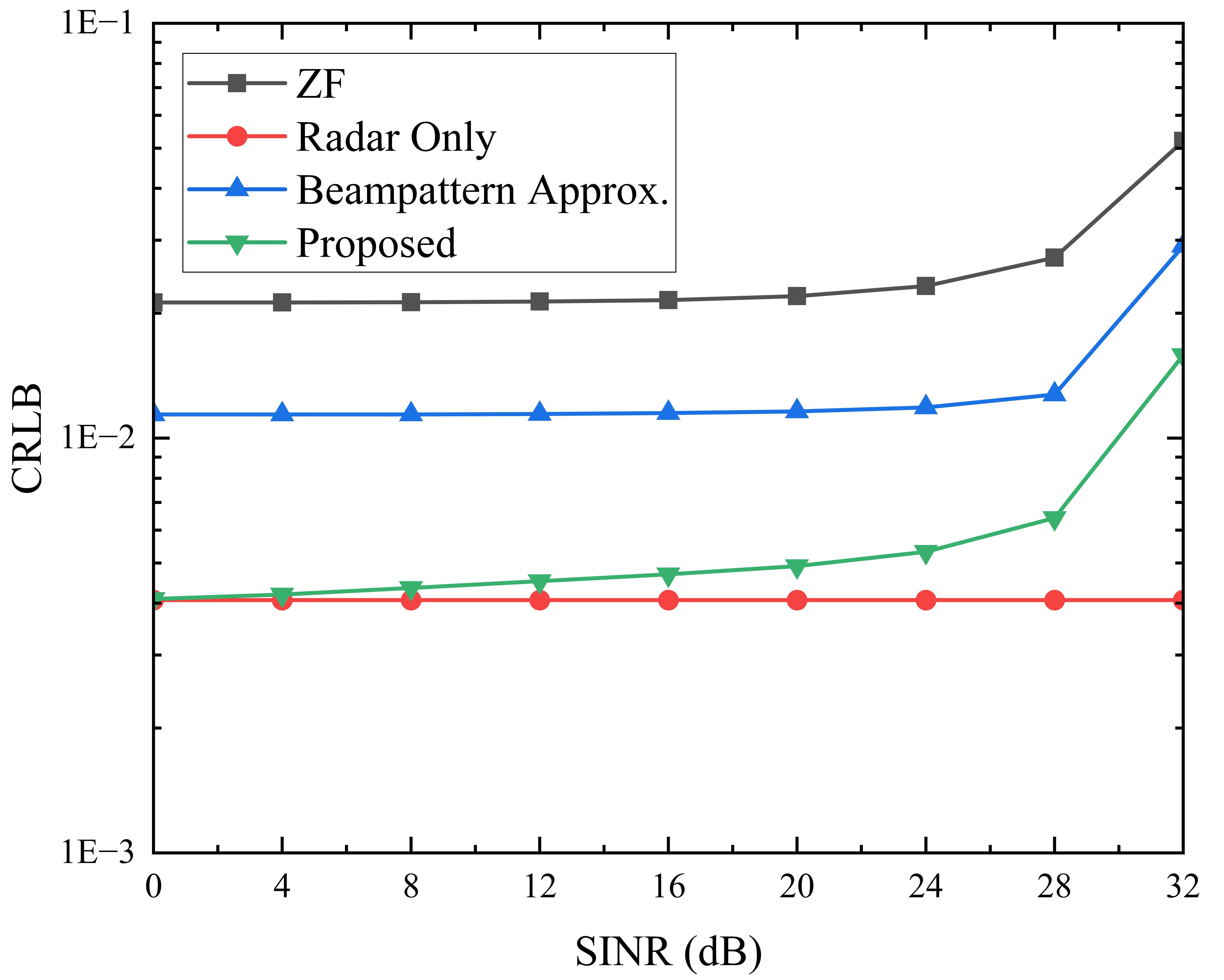
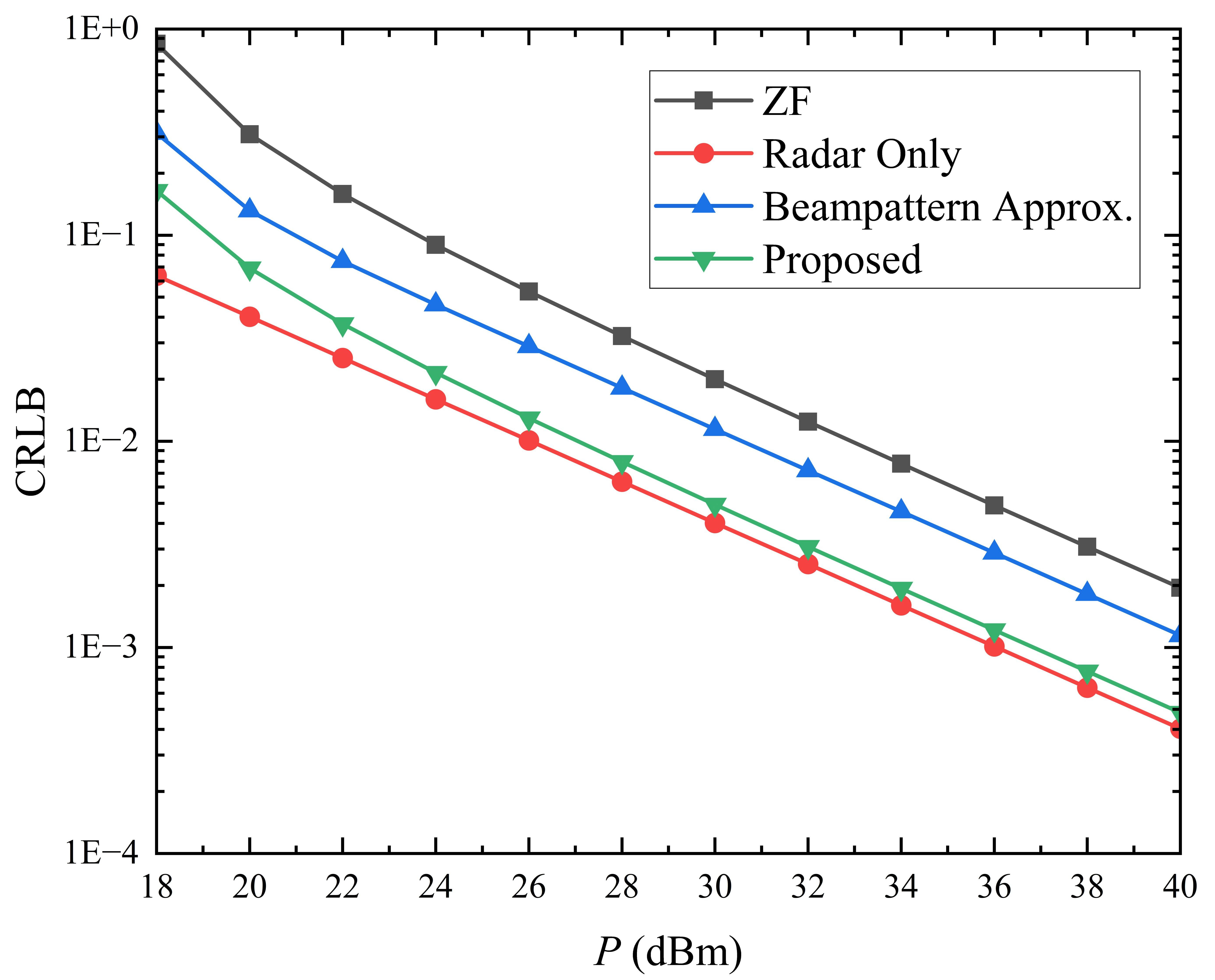
Fig. 3 compares the CRLB performance versus the transmit power . The proposed algorithm consistently surpasses the performance of both the ZF and beampattern approximation algorithms, irrespective of the magnitude of . Furthermore, an intriguing trend is observed regarding the performance disparity between the proposed algorithm and the radar only beamforming algorithm. Specifically, this gap widens as diminishes. The underlying reason is that the ISAC system must allocate a sufficient portion of the transmit power to communication to ensure the maintenance of the communication rate. Consequently, this necessitates a reduction in the power allocated to the sensing when is constrained, highlighting the critical trade-off between target localization accuracy and communication SINR.
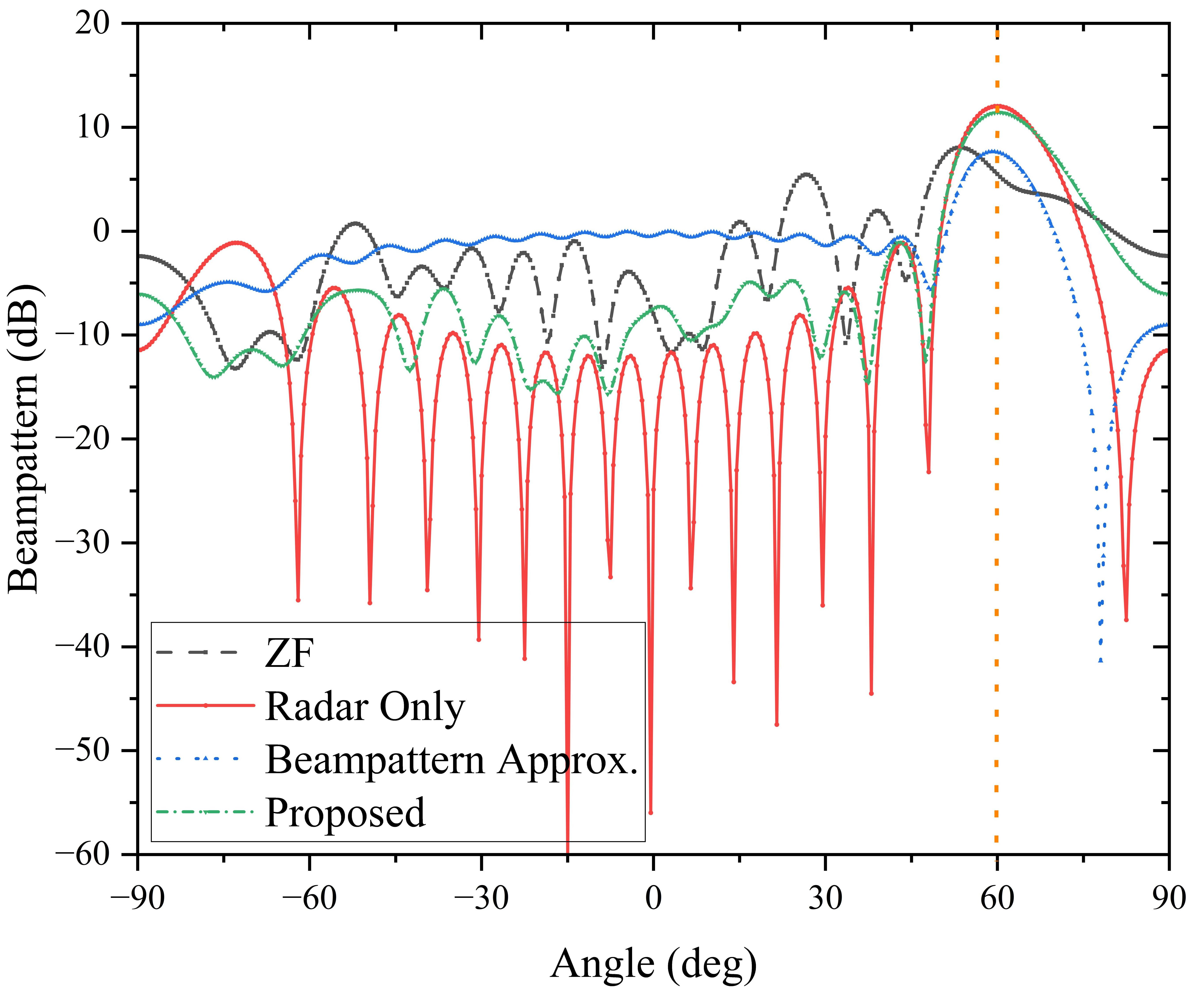
The resultant beampatterns for all considered algorithms in BS 1 are depicted in Fig. 4. Within this simulation, the target is positioned at angle of relative to the BS. Observations reveal that the proposed beamforming algorithm successfully generate the desired beampattern, with its main lobe aligned at , mirroring the performance of the radar only beamforming algorithm. However, the beampattern approximation algorithm does not achieve the similar level of sharpness in the main lobe as the proposed algorithm. Moreover, the ZF algorithm fails to form directional beams towards the target direction, underscoring its inadequacy for radar sensing applications. These simulation outcomes align with the CRLB performance results presented in Fig. 2 and Fig. 3, further validating the efficiency and suitability of the proposed beamforming algorithm for multi-cell integrated localization and communication systems.
V Conclusion
In this paper, we studied the integrated localization and communication problem in a multi-cell system. We derived two key performance indicators: the SINR for communication and the CRLB for target localization. Exploiting the established performance metrics, we formulated a nonconvex optimization problem to minimize the CRLB while maintaining the communication SINR. We proposed a coordinated beamforming algorithm to solve this problem based on the SDR strategy, and show that the SDR is always tight under mild conditions. Through numerical simulations, we verified the effectiveness of the proposed algorithm, and show the trade-off between communication SINR and the CRLB of target localization, providing valuable insights for the design of future multi-cell ISAC systems.
Appendix A Proof of Lemma 2
References
- [1] W. Xu, Y. Huang, W. Wang et al., “Toward ubiquitous and intelligent 6G networks: From architecture to technology,” Sci. China Inf. Sci., vol. 66, no. 3, pp. 130 300:1–2, Mar. 2023.
- [2] W. Xu, Z. Yang, D. W. K. Ng et al., “Edge learning for B5G networks with distributed signal processing: Semantic communication, edge computing, and wireless sensing,” IEEE J. Sel. Topics Signal Process., vol. 17, no. 1, pp. 9–39, Jan. 2023.
- [3] W. Xu, J. Wu, S. Jin et al., “Disentangled representation learning empowered CSI feedback using implicit channel reciprocity in FDD massive MIMO,” IEEE Trans. Wireless Commun., vol. 23, no. 10, pp. 15169-15184, Oct. 2024.
- [4] G. Chen, R. Zhang, H. Ren et al., “Joint beamforming design for dual-functional radar-communication systems under beampattern gain constraints,” ZTE Commun., vol. 22, no. 3, pp. 13–20, Sep. 2024.
- [5] F. Liu, Y. Cui, C. Masouros et al., “Integrated sensing and communications: Toward dual-functional wireless networks for 6G and beyond,” IEEE J. Sel. Areas Commun., vol. 40, no. 6, pp. 1728–1767, Jun. 2022.
- [6] C. Sturm and W. Wiesbeck, “Waveform design and signal processing aspects for fusion of wireless communications and radar sensing,” Proc. IEEE, vol. 99, no. 7, pp. 1236–1259, Jul. 2011.
- [7] X. Liu, T. Huang, N. Shlezinger et al., “Joint transmit beamforming for multiuser MIMO communications and MIMO radar,” IEEE Trans. Signal Process., vol. 68, pp. 3929–3944, Jun. 2020.
- [8] Z. He, W. Xu, H. Shen et al., “Full-duplex communication for ISAC: Joint beamforming and power optimization,” IEEE J. Sel. Areas Commun., vol. 41, no. 9, pp. 2920–2936, Sep. 2023.
- [9] L. Xie, P. Wang, S. Song et al., “Perceptive mobile network with distributed target monitoring terminals: Leaking communication energy for sensing,” IEEE Trans. Wireless Commun., vol. 21, no. 12, pp. 10193–10207, Dec. 2022.
- [10] G. Cheng, Y. Fang, J. Xu et al., “Optimal coordinated transmit beamforming for networked integrated sensing and communications,” IEEE Trans. Wireless Commun., vol. 23, no. 8, pp. 8200-8214, Jan. 2024.
- [11] Y. Chen, L. Zhao, and K. Shen, “Fast fractional programming for multi-cell integrated sensing and communications,” 2024, arXiv:2406.10910.
- [12] X. Wang, Z. Fei, J. A. Zhang et al., “Constrained utility maximization in dual-functional radar-communication multi-UAV networks,” IEEE Trans. Commun., vol. 69, no. 4, pp. 2660–2672, Apr. 2021.
- [13] Y. Huang, Y. Fang, X. Li et al., “Coordinated power control for network integrated sensing and communication,” IEEE Trans. Veh. Technol., vol. 71, no. 12, pp. 13361–13365, Dec. 2022.
- [14] H. Godrich, A. M. Haimovich, and R. S. Blum, “Target localization accuracy gain in MIMO radar-based systems,” IEEE Trans. Inf. Theory, vol. 56, no. 6, pp. 2783–2803, Jun. 2010.
- [15] Z. Q. Luo, W. K. Ma, A. M. C. So et al., “Semidefinite relaxation of quadratic optimization problems,” IEEE Signal Process. Mag., vol. 27, no. 3, pp. 20–34, May 2010.
- [16] P. G. Stoica and R. Moses, Spectral Analysis of Signals. Upper Saddle River, NJ: Pearson, Prentice Hall, 2005.
- [17] N. H. Lehmann, A. M. Haimovich, R. S. Blum et al., “High resolution capabilities of MIMO radar,” in Proc. Asilomar Conf. Signals, Syst., Comput. (ACSSC), Pacific Grove, CA, USA, Oct. 2006, pp. 25–30.