Existence and stability of ground states for the defocusing Nonlinear Schrödinger equation on Quantum Graphs

Abstract.

We study the existence and stability of ground states for the defocusing nonlinear Schrödinger equation on non-compact metric graphs. We establish a sharp criterion for the existence of action ground states, linking it to the spectral properties of the Hamiltonian operator. In particular, we show that ground states exist if and only if the bottom of the spectrum of the Hamiltonian is negative and the frequency lies in a suitable range. Furthermore, we investigate the relationship between action and energy ground states, proving that while every action minimizer is an energy minimizer, the converse may not hold and the energy minimizer may not exist for all masses. To illustrate this phenomenon, we analyze explicit solutions on star graphs with $\delta$ and $\delta^{\prime}$-couplings, showing that for mass subcritical exponents of the nonlinearity, there exists a large interval of masses for which no energy ground state exists while in the opposite case, they exist for all masses.

1. Introduction

Quantum graphs, which model wave propagation in networks, have gained significant attention in mathematical physics and nonlinear analysis. In particular, the nonlinear Schrödinger equation (NLS) on quantum graphs provides a fundamental framework for studying nonlinear wave phenomena in branched structures, which arise naturally in diverse fields such as optics [6, 35] and condensed matter physics [10, 12, 13].

In this work, we investigate the defocusing nonlinear Schrödinger equation on a metric graphs, where the underlying differential operator $\operatorname{H}$ is given by a Laplacian, incorporating generic vertex conditions, discussed in [8, Chapter $1$] and Section 2 below. More specifically, we analyze the defocusing nonlinear Schrödinger equation on a non-compact metric graph $\mathcal{G}$. We define as non-compact graph, a graph which consists of a finite set of edges $\mathcal{E}$ and vertices $\mathcal{V}$, where at least one edge has an infinite length.

We consider the operator $\operatorname{H}$ acting as the usual Laplacian on each edge

$$\operatorname{H}\psi=(-\psi_{e}^{\prime\prime})_{e\in\mathcal{E}}$$

and endowed with proper vertex conditions on each vertex $v\in\mathcal{V}$ as in [8, Chapter $1$] coming from the Shapiro-Lopatinski theory [36]. In order to present the problem, we also introduce the associated quadratic form

$$Q_{\operatorname{H}}(\psi)=\langle\operatorname{H}\psi,\psi\rangle_{L^{2}(\mathcal{G})}$$

and denote by $D(Q_{\operatorname{H}})$ its domain. In general, depending on the vertex conditions, the domain $D(Q_{\operatorname{H}})$ is a subset of $H^{1}(\mathcal{G})$, see the discussion in Section 2, where we give the precise definition of the operator $\operatorname{H}$ as well as Lebesgue and Sobolev spaces for $\mathcal{G}$.

We consider the defocusing nonlinear Schrödinger equation

(1) $$\begin{cases}i\partial_{t}u=\operatorname{H}u+|u|^{p-1}u,\\ u(t=0)=u_{0}\in D(Q_{\operatorname{H}})\end{cases}$$

for $u:\mathbb{R}\times\mathcal{G}\to\mathbb{C}$ and $p>1$. The initial datum $u_{0}$ belongs to the energy space $D(Q_{\operatorname{H}})$ ensuring well-posedness of (1) by the classical contraction principle argument [14]. Global well-posedness follows from the conservation of the two functionals $E,M:D(Q_{\operatorname{H}})\to\mathbb{R}$ called respectively the energy and the mass and given by

(2) $$E(\psi)=\frac{1}{2}Q_{\operatorname{H}}(\psi)+\frac{1}{p+1}\|\psi\|_{L^{p+1}(\mathcal{G})}^{p+1},\quad\quad M(\psi)=\frac{1}{2}\|\psi\|_{L^{2}(\mathcal{G})}^{2}$$

We will primarily focus on the associated stationary problem, which arises by making the standard ansatz

$$u(t)=e^{i\omega t}\psi,$$

where $\omega\in\mathbb{R}$ represents the frequency parameter, and $\psi$ is a time-independent function belonging to $D(Q_{\operatorname{H}})$. Substituting this ansatz into the time-dependent equation (1) reduces the problem to the stationary defocusing nonlinear Schrödinger equation

(3) $$\operatorname{H}\psi+\omega\psi+|\psi|^{p-1}\psi=0.$$

This equation governs the standing wave solutions of the system. Solutions to this equation can be seen as critical points of the action functional $S_{\omega}:D(Q_{\operatorname{H}})\to\mathbb{R}$ defined by

$$S_{\omega}(\psi) =E(\psi)+\omega M(\psi)$$

We consider the variational problem

(4) $$s_{\omega}=\inf\left\{S_{\omega}(\psi):\psi\in D(Q_{\operatorname{H}})\setminus\{0\}\right\}.$$

If a minimizer exists it will be a solution to $S^{\prime}_{\omega}(u)=0$, that is, as said before, the equation (3). We denote the set of all minimizers to (4) as

(5) $$\mathcal{A}_{\omega}=\{\psi\in D(Q_{\operatorname{H}}):S_{\omega}(\psi)=s_{\omega}\}$$

and we refer to them as action ground states. Another classical way to obtain solutions to (3) is to consider, for $m>0$, the minimization problem

(6) $$e_{m}=\inf\{E(\psi):\psi\in D(Q_{\operatorname{H}}),\,M(\psi)=m\}.$$

In this case, the parameter $\omega$ in (3) arises as a Lagrangian multiplier. A natural question is whether the infimum $e_{m}$ is attained, i.e., whether there exists a function $\psi\in D(Q_{\operatorname{H}})$ such that $M(\psi)=m$ and $E(\psi)=e_{m}$. We will refer to these functions as energy ground states and denote the set by $\mathcal{B}_{m}$, so

(7) $$\mathcal{B}_{m}=\{\psi\in D(Q_{\operatorname{H}}):E(\psi)=e_{m},\ M(\psi)=m\}.$$

Our primary objective in this work is to establish a necessary and sufficient condition for the existence of action ground states. Before proceeding with our analysis, we first review the relevant literature on the subject.

Quantum graphs provide a simplified one-dimensional model for studying wave propagation in fiber-like structures. Their effectiveness in approximating higher-dimensional counterparts has been investigated in [31, 32]. In [42], a connection was established between energy/mass minimizers on product spaces and ground states on $\mathbb{R}^{d}\times\mathcal{M}$ where $\mathcal{M}$ is a compact manifold. The Gross-Pitaevskii equation on $\mathbb{R}\times\mathbb{T}$ with a general nonlinearity was recently studied in [18, 38], where it was shown that energy/momentum minimizers become effectively one-dimensional as the torus $\mathbb{T}$ shrinks to zero. The bifurcation between a one-dimensional line soliton and a fully two-dimensional soliton on the cylinder $\mathbb{R}\times\mathbb{T}$ was analyzed in [7, 44, 45] More recently in [34] a line with a $\delta$ -potential was obtained as the limiting case of a fractured strip $\mathbb{R}\times[0,L]$ with Neumann boundary conditions.

The study of the nonlinear Schrödinger equation on quantum graphs has gained significant attention over the past two decades, particularly in the case of the focusing nonlinearity (where the nonlinear term appears with a minus sign). In this setting, numerous works have investigated the existence of standing waves and their stability. The first contribution can be reconnected to the case of the line with a delta potential, as an example of a star-graph with two edges. In this case, the works [21, 22, 24] establish the existence of action ground states and their stability, and in [33] the full picture of stability and instability is provided for different choice of parameters in the equation. For the energy minimizers, the existence of energy ground states is proven in [3] on the line with a quadratic form which includes those considered here.

Similar results were later obtained in more general graphs. Notably, the classical concentration compactness principle of Lions [37] is slightly modified for the graphs. Specifically, in addition to the three standard behaviors of vanishing, compactness, and dichotomy, an additional possible behavior must be accounted for, the run-away, where mass escapes to infinity on one infinite edge, see [1]. This gives rise to a general criterion of existence for both energy and action ground states on graphs. Roughly speaking, if the energy (or the action) of the line ground state is superior to one of possible candidates for the minimization problem, then a ground state exists as the run-away behavior can be ruled out. Then vanishing and dichotomy are ruled out due the convexity of the energy. Due to this criterion, existence of energy ground states is proven in [1, 2, 4, 5, 11, 17]. For a general recent review on the focusing NLS on quantum graphs, we refer to [28].

In contrast, the defocusing case has received significantly less attention, despite its mathematical and physical relevance [41]. The present work aims to contribute to bridging this gap.

In $\mathbb{R}$, it is well known that for $\operatorname{H}=-\partial_{xx}$, $H^{1}(\mathbb{R})$ solutions to (3) do not exist. However, in bounded domains, solutions to the defocusing stationary equation do exist under various boundary conditions. This follows from the compact Sobolev embedding $H^{1}(I)\hookrightarrow L^{p}(I)$ for any $p\in[2,\infty]$ and classical variational methods, which will be discussed later in this work (see for example [26]).

Quantum graphs lie at the interface of these two settings, combining features of both bounded and unbounded domains. This makes them an interesting framework to investigate. To our knowledge, the defocusing stationary NLS on graphs has been addressed in only two works. In [29], the case of the real line with a negative delta potential was analyzed, leading to the proof of existence and uniqueness (up to a phase shift) of solutions to (3). This result was later extended in [40] to star graphs.

Given the scarcity of results in the defocusing case, our goal is to further develop the theory by considering a general non-compact quantum graph with arbitrary vertex conditions discussed in Section 2. We will then consider two specific cases in Section 4, that is the cases of a star graph with $\delta$ or $\delta^{\prime}$ condition on the vertex.

The defocusing case differs from the focusing case in several ways. In particular, minimizing the action functional does not require additional constraints, such as working on the Nehari manifold. As a result, searching for action minimizers is more straightforward than identifying energy ground states.

Moreover, due to the local nature of the vertex conditions, the problem of finding an action ground state primarily reduces to preventing vanishing by scaling. Consequently, the existence criterion in this setting simplifies to the condition $s_{\omega}<0$.

Since the only possible negative contribution to the action comes from the quadratic form, the criterion implies that the choice of vertex conditions and $\omega$ must be carefully made. In particular, defining $l_{\operatorname{H}}$ as the bottom of the spectrum of $\operatorname{H}$,

(8) $$l_{\operatorname{H}}=\inf\left\{\left\langle\operatorname{H}\psi,\psi\right\rangle_{L^{2}(\mathcal{G})}:\psi\in D(Q_{\operatorname{H}}),\|\psi\|_{L^{2}(\mathcal{G})}=1\right\},$$

a necessary condition for the existence of an action minimizer is $l_{\operatorname{H}}<0$. In our main result, we will show that, as long as one chooses $\omega\in(0,-l_{\operatorname{H}})$, this becomes also a sufficient condition for existence on the ground states.

Theorem 1.1.

Let $\mathcal{G}$ be a non-compact metric graph. An action ground state exists if and only if $l_{\operatorname{H}}<0$ and $\omega\in(0,-l_{\operatorname{H}})$.

Thus, the existence of action ground states for the nonlinear model reduces to analyzing the spectral properties of the Hamiltonian operator $\operatorname{H}$. For star graphs, a criterion for the existence of a negative eigenvalue of the Hamiltonian is provided in [30, Theorem 3.7]. In the case of graphs containing at least one compact edge, [30, Theorem 3.2] establishes a criterion for determining whether a given scalar $l\in\mathbb{C}$ is an eigenvalue of $\operatorname{H}$.

As a consequence of the conservation of the action, we will also obtain the stability of the set $\mathcal{A}_{\omega}$ for the equation (1). A set $\mathcal{A}$ is said to be stable if for any $\varepsilon>0$, there exists $\eta>0$ such that if $u_{0}\in D(Q_{\operatorname{H}})$ satisfies

$$\inf_{\psi\in\mathcal{A}}\|u_{0}-\psi\|_{H^{1}(\mathcal{G})}<\eta,$$

then the corresponding solution $u$ to (1) satisfies

$$\sup_{t\geq 0}\inf_{\psi\in\mathcal{A}}\|u(t,\cdot)-\psi\|_{H^{1}(\mathcal{G})}<\varepsilon.$$

Finally, we will also show that the function $\omega\mapsto s_{\omega}$, defined for $\omega\in(0,-l_{\operatorname{H}})$ is continuous and strictly increasing.

Corollary 1.2.

Let $l_{\operatorname{H}}<0$ and $\omega\in(0,-l_{\operatorname{H}})$. Then the function $\omega\mapsto s_{\omega}$ is continuous and strictly increasing and the set $\mathcal{A}_{\omega}$ is stable.

In contrast to action ground states, the existence of energy ground states for the defocusing NLS is significantly more challenging. Notably, the energy functional is no longer convex for all masses. In some cases, the minimization problem (6) satisfies $e_{m}>-\infty$, yet no minimizer exists due to the possibility of dichotomy in the concentration-compactness argument. In other words, an energy minimizer may not exist for a given mass $m>0$, as its existence depends on the structure of the graph and the parameters in equation (3). A concrete example illustrating this phenomenon will be presented in Section 4.

Another key difference from the focusing case lies in the relationship between action and energy ground states. In the focusing case, energy minimizers typically also minimize the action. However, the conditions under which the reverse holds remain unclear. For further discussion on this, we refer to [16, 19, 27].

In our setting, the situation is reversed: every action ground state is also an energy ground state. However, the converse is more difficult to establish, as the relationship between the parameter $\omega$ and the mass of action ground states remains unclear. As a first step in addressing this issue, we demonstrate that this question is linked to the uniqueness of energy minimizers. Specifically, we prove that if two distinct energy minimizers exist and have two different associated Lagrangian multipliers, then at least one of them cannot be an action minimizer.

Theorem 1.3.

Let $\omega\in(0,-l_{\operatorname{H}})$ and $\phi\in\mathcal{A}_{\omega}$ with $m=M(\phi)$ . Then $\phi\in\mathcal{B}_{m}$.

Moreover, if for some $m>0$, there exist two distinct functions $\psi\neq\phi$ such that $\psi,\phi\in\mathcal{B}_{m}$ and their associated Lagrange multipliers satisfy $\omega_{\psi}\neq\omega_{\phi}$, then either $\psi\notin\mathcal{A}_{\omega_{\psi}}$ or $\phi\notin\mathcal{A}_{\omega_{\phi}}$.

In Section 3, we will prove Theorems 1.1 and 1.3, along with additional properties of ground states. Section 4 then focuses on the specific case of a star graph with $\delta$- or $\delta^{\prime}$ -couplings. Section 4 serves two main purposes.

First, in this setting, explicit solutions to (3) are available and are unique up to a phase shift. The explicit solution for the $\delta$ -coupling was derived in [40], while we will compute the solution for the $\delta^{\prime}$ -coupling.

Second, exploiting these explicit solutions, we will demonstrate that for $p<5$ , there exists a large interval of masses for which no energy ground state exists. Specifically, we will show that there exists a threshold $m_{p}$ with $m_{p}=\infty$ for $p\geq 5$ and $m_{p}<\infty$ for $p\in(1,5)$ such that energy ground states exist only for $m\in(0,m_{p})$. This is shown in Proposition 4.4.

The remainder of this paper is organized as follows. In Section 2, we introduce the necessary notation and preliminaries, including the spectral properties of the operator $\operatorname{H}$ and the well-posedness of problem (1). In Section 3, we establish the proof of Theorem 1.1, providing a rigorous criterion for the existence of ground states. Finally, in Section 4, we focus on the specific case of the star graph with $\delta$ and $\delta^{\prime}$ coupling at the vertex, which is of particular interest as it allows for the construction of explicit solutions, providing deeper insights into the analytical properties of ground states.

2. Preliminaries

2.1. Metric graphs

In this paper, we consider a metric graph $\mathcal{G}=(\mathcal{E},\mathcal{V})$, with $\mathcal{E}$ the set of edges and $\mathcal{V}$ the set of vertices. The sets $\mathcal{E}$ and $\mathcal{V}$ will always be supposed of finite cardinality. For $v\in\mathcal{V}$, we denote by $J_{v}$ the set of edges adjacent to $v$ and by $d_{v}$ the cardinal of $J_{v}$. An edge $e\in\mathcal{E}$ has a length $L_{e}$ that can be finite or infinite. The coordinate system on the metric graph is largely arbitrary. When the length $L_{e}$ is finite, the edge $e\in\mathcal{E}$ can be identified with a different choice for an interval $I_{e}\subset\mathbb{R}$, as for example $I_{e}=[0,L_{e}]$. When the length $L_{e}$ is infinite, the edge can be identified with any half-line $I_{e}=[a,\infty)$, where $a\in\mathbb{R}$ can be chosen freely. We highlight that throughout this work, every graph $\mathcal{G}$ considered has at least one infinite edge. For a later convenience, we define as $L$ as the minimum between half of the minimum length between every edge and $1/2$

(9) $$L=\frac{1}{2}\min\left(\min_{e\in\mathcal{E}}L_{e},1\right).$$

This quantity is well defined and $L>0$ since $|\mathcal{E}|<\infty$. A point $\tilde{x}\in\mathcal{G}$ on the graph can be identified by giving the edge $e\in\mathcal{E}$ and the coordinate $x$ on the edge: $\tilde{x}=(e,x)$. With slight abuse of notation we will use $x$ for both a point on the graph and a coordinate on one edge when there is no ambiguity.

A function on the metric graph is defined component-wise, giving its value on any edge. Assigning $\psi$ on $\mathcal{G}$ corresponds to specifying its edge components $\{\psi_{e}\}_{e\in E}$, where each $\psi_{e}$ is a function $\psi_{e}:I_{e}\to\mathbb{C}$. Equivalently, for a point $\tilde{x}=(e,x)$ on the graph, we define $\psi(\tilde{x})=\psi_{e}(x)$. Since a general metric graph $\mathcal{G}$ is described by a collection of points and intervals, a natural choice of metric structure on $\mathcal{G}$ is given by the Lebesgue spaces defined on these intervals. In particular, if a function $\psi$ is integrable, then every component $\psi_{e}$ on the edge is integrable on $I_{e}$ and

$$\int_{\mathcal{G}}\psi(x)dx=\sum_{e\in\mathcal{E}}\int_{I_{e}}\psi_{e}(x)dx.$$

For $p\geq 2$ and $k\in\mathbb{N}$, this allows to define the Lebesgue and Sobolev spaces

$$L^{p}(\mathcal{G})=\bigoplus_{e\in\mathcal{E}}L^{p}(I_{e}),\quad H^{k}(\mathcal{G})=\bigoplus_{e\in\mathcal{E}}H^{k}(I_{e})$$

endowed with the norms given by

$$\left\|\psi\right\|_{L^{p}(\mathcal{G})}^{p}=\sum_{e\in\mathcal{E}}\left\|\psi_{e}\right\|_{L^{p}(I_{e})}^{p},\quad\left\|\psi\right\|_{H^{k}(\mathcal{G})}^{2}=\sum_{e\in\mathcal{E}}\left\|\psi_{e}\right\|_{H^{k}(I_{e})}^{2},$$

and the scalar product on $L^{2}(\mathcal{G})$ as

$$\langle\psi,\phi\rangle_{L^{2}(\mathcal{G})}=\operatorname{Re}\left(\int_{\mathcal{G}}\psi(x)\overline{\phi(x)}dx\right)=\sum_{e\in\mathcal{E}}\operatorname{Re}\left(\int_{I_{e}}\psi_{e}(x)\overline{\phi_{e}(x)}dx\right).$$

For $\psi\in H^{1}(\mathcal{G}),v\in\mathcal{V}$ and $e\in J_{v}$, we denote by $\psi_{e}(v)$ the value of $\psi_{e}$ at the vertex $v$ and by $\Psi(v)\in\mathbb{C}^{d_{v}}$ the vector given by

$$\Psi(v)=(\psi_{e_{1}}(v),\ldots,\psi_{e_{d_{v}}}(v)),$$

where $\{e_{1},\dots,e_{d_{v}}\}=J_{v}$. For $q\in[2,\infty]$ and $\psi\in H^{1}(\mathcal{G})$, the Gagliardo–Nirenberg inequality

(10) $$\|\psi\|_{L^{q}(\mathcal{G})}\leq C\|\psi^{\prime}\|_{L^{2}(\mathcal{G})}^{\frac{1}{2}-\frac{1}{q}}\|\psi\|_{L^{2}(\mathcal{G})}^{\frac{1}{2}+\frac{1}{q}}$$

holds for some $C>0$ [23, 39]. Furthermore, the standard Sobolev inequalities hold on $\mathcal{G}$ in the same form as in the classical case.

2.2. Hamiltonian operator

A comprehensive introduction of the Hamiltonian operator is given in [8, Chapter 1]. We equip the metric graph $\mathcal{G}$ with the operator $\operatorname{H}:L^{2}(\mathcal{G})\to L^{2}(\mathcal{G})$, called the Hamiltonian operator, acting as

$$\operatorname{H}\psi=(-\psi_{e}^{\prime\prime})_{e\in\mathcal{E}}$$

and defined on a subdomain of $H^{2}(\mathcal{G})$ including local vertex conditions of the form

$$A_{v}\Psi(v)+B_{v}\Psi^{\prime}(v)=0$$

for all $v\in\mathcal{V}$, where $A_{v}$ and $B_{v}$ are $(d_{v}\times d_{v})$-matrices. The domain of $\operatorname{H}$ is given by

$$D(\operatorname{H})=\left\{\psi\in H^{2}(\mathcal{G}):A_{v}\Psi(v)+B_{v}\Psi^{\prime}(v)=0\text{ for all }v\in\mathcal{V}\right\}.$$

A self-adjointness criterion for $\operatorname{H}$ is the following.

Proposition 2.1.

The following assertions are equivalent:

1. The operator $\operatorname{H}$ is self-adjoint.

2. For every $v\in\mathcal{V}$, the matrices $A_{v}$ and $B_{v}$ satisfy the following conditions: the $(d_{v}\times 2d_{v})$-matrix $(A_{v},B_{v})$ has maximal rank and the matrix $A_{v}B_{v}$ is symmetric.

3. For every $v\in\mathcal{V}$, there are three orthogonal and mutually orthogonal projectors $P_{D,v},P_{N,v}$ and $P_{R,v}=I_{d_{v}}-P_{D,v}-P_{N,v}$ acting on $\mathbb{C}^{d_{v}}$ and an invertible symmetric matrix $\Lambda_{v}$ acting on the subspace $P_{R,v}\mathbb{C}^{d_{v}}$ such that, for $\psi\in D(\operatorname{H})$,

   $$P_{D,v}\Psi(v)=0,\quad P_{N,v}\Psi^{\prime}(v)=0,\quad P_{R,v}\Psi^{\prime}(v)=\Lambda_{v}P_{R,v}\Psi(v).$$

In what follows, the operator $\operatorname{H}$ is always supposed to be self-adjoint. Its quadratic form $Q_{\operatorname{H}}$ is given by

(11) $$Q_{\operatorname{H}}(\psi) =\langle\operatorname{H}\psi,\psi\rangle_{L^{2}(\mathcal{G})}=\|\psi^{\prime}\|_{L^{2}(\mathcal{G})}^{2}+\sum_{v\in\mathcal{V}}\langle\Lambda_{v}P_{R,v}\Psi(v),P_{R,v}\Psi(v)\rangle_{\mathbb{C}^{d_{v}}}.$$

It is defined on the domain

(12) $$D(Q_{\operatorname{H}})=\left\{\psi\in H^{1}(\mathcal{G}):P_{D,v}\Psi(v)=0\text{ for all }v\in\mathcal{V}\right\},$$

called the energy space. We denote by $D(Q_{\operatorname{H}})^{\star}$ its topological dual. Observe that the quadratic form comprises two parts: the $L^{2}(\mathcal{G})$-norm of the derivative of the function and a quadratic part coming from the vertex conditions. The following lemma holds.

Lemma 2.2.

Let $(\psi_{n})_{n\in\mathbb{N}}\subset D(Q_{\operatorname{H}})$ be a sequence bounded in $H^{1}(\mathcal{G})$. Then, there exists $\psi\in D(Q_{\operatorname{H}})$ such that $\psi_{n}\rightharpoonup\psi$ as $n\to\infty$ weakly in $H^{1}(\mathcal{G})$ up to a subsequence. Furthermore, for $v\in\mathcal{V}$, we have

(13) $$\sum_{v\in\mathcal{V}}\langle\Lambda_{v}P_{R,v}\Psi_{n}(v),P_{R,v}\Psi_{n}(v)\rangle_{\mathbb{C}^{d_{v}}}\to\sum_{v\in\mathcal{V}}\langle\Lambda_{v}P_{R,v}\Psi(v),P_{R,v}\Psi(v)\rangle_{\mathbb{C}^{d_{v}}}\text{ as $n\to\infty$}$$

up to a subsequence.

Proof.

Let $\psi\in H^{1}(\mathcal{G})$ be such that $\psi_{n}\rightharpoonup\psi$ as $n\to\infty$ weakly in $H^{1}(\mathcal{G})$ up to a subsequence. Let $v\in\mathcal{V}$ and $e\in J_{v}$. The compact embedding $H^{1}(v,L)\subset C\left([v,L]\right)$ holds, where $L$ has been defined in (9). Therefore, we have $\psi_{n,e}(v)\to\psi_{e}(v)$ as $n\to\infty$ up to a subsequence, so that $\Psi_{n}(v)\to\Psi(v)$ as $n\to\infty$. In particular, $P_{D,v}\Psi(v)=0$, so $\psi\in D(Q_{\operatorname{H}})$. As

$$\left|\langle\Lambda_{v}P_{R,v}\Psi(v),P_{R,v}\Psi(v)\rangle_{\mathbb{C}^{d_{v}}}\right|\lesssim\sum_{v\in\mathcal{V}}\sum_{e,e^{\prime}\in J_{v}}|\psi_{e}(v)||\psi_{e^{\prime}}(v)|,$$

we obtain (13), and this concludes the proof. ∎

We also show that the essential spectrum of $\operatorname{H}$ is given by $[0,\infty)$. This result can be proven by the classical Weyl’s theorem [43, Theorem $6.19$] and has been shown under several different settings, as for example for star-graphs in [25, Proposition $3.2$]. We present a slightly alternative proof which covers all the relevant settings in our work. The idea of the proof is to compute first the essential spectrum of the Hamiltonian operator with Dirichlet-vertex conditions and then to deduce the essential spectrum of $\operatorname{H}$ through the computation of a Weyl’s sequence.

Proposition 2.3.

The essential spectrum of $\operatorname{H}$ is given by $\sigma_{ess}(\operatorname{H})=[0,\infty)$.

Proof.

Step 1: We introduce the Hamiltonian operator $\operatorname{H}_{D}$ with Dirichlet-vertex conditions, defined on the domain

$$D(\operatorname{H}_{D})=\left\{\psi\in H^{2}(\mathcal{G}):\psi_{e}(v)=0\text{ for all }v\in\mathcal{V},e\in J_{v}\right\}.$$

This operator is self-adjoint (see [8, Chapter $1$]) and, for $\psi\in D(\operatorname{H}_{D})$, we have

$$\langle\operatorname{H}_{D}\psi,\psi\rangle_{L^{2}(\mathcal{G})}=\operatorname{Re}\left(\int_{\mathcal{G}}|\psi^{\prime}(x)|^{2}dx\right)\geq 0.$$

Thus, $\sigma(\operatorname{H}_{D})\subset[0,\infty).$ To show the reverse inclusion, we consider $\lambda\in\rho(\operatorname{H}_{D})$, where $\rho(\operatorname{H}_{D})$ denotes the resolvent set of $\operatorname{H}_{D}$. For all $\psi\in L^{2}(\mathcal{G})$, there exists a unique $\phi\in D(\operatorname{H}_{D})$ such that, for all $e\in\mathcal{E}$,

$$(-\partial_{xx}-\lambda)^{-1}\psi_{e}(x)=\phi_{e}(x),\quad x\in I_{e}.$$

Let $e\in\mathcal{E}$ such that $L_{e}=\infty$. We extend $\psi_{e}$ (respectively $\phi_{e}$) by central symmetry on $\mathbb{R}$, and we denote its extension by $\tilde{\psi}_{e}$ (respectively $\tilde{\phi}_{e}$), that is

(14) $$\tilde{\psi}_{e}(x)=\begin{cases}\psi_{e}(x)\quad\ \ \,x\geq 0,\\ \psi_{e}(-x)\quad x<0,\end{cases}$$

and the same for $\tilde{\phi}_{e}$ so that $\tilde{\psi}_{e}\in L^{2}(\mathbb{R})$ and $\tilde{\phi}_{e}\in H^{2}(\mathbb{R})$. Then, $\tilde{\phi}_{e}$ is the only function in $H^{2}(\mathbb{R})$ (up by multiplication by a constant) which satisfies

$$(-\partial_{xx}-\lambda)^{-1}\tilde{\psi}_{e}(x)=\tilde{\phi}_{e}(x),\quad x\in\mathbb{R},$$

otherwise this would contradict the fact that $\phi$ is the unique preimage of $\psi$ under the operator $(\operatorname{H}_{D}-\lambda)^{-1}$. In particular, the unbounded operator $(-\partial_{xx}-\lambda)$ defined on the domain $\left\{\psi\in H^{2}(\mathbb{R}):f(0)=0\right\}\subset L^{2}(\mathbb{R})$ is invertible. This operator has no discrete spectrum and its essential spectrum is given by $[0,\infty)$. Therefore, $\lambda\in\mathbb{C}\setminus[0,\infty)$ and finally

(15) $$\sigma_{ess}(\operatorname{H}_{D})=[0,\infty).$$

Step 2: Let $\lambda\in\sigma_{ess}(\operatorname{H})$. From [20, Chapter $9$], there exists a Weyl’s sequence $(\phi_{n})_{n\in\mathbb{N}}\subset D(\operatorname{H})$, i.e. the sequence satisfies the following conditions:

(16) $$\|\phi_{n}\|_{L^{2}(\mathcal{G})}=1\text{ for all }n\in\mathbb{N},$$

(17) $$\phi_{n}\rightharpoonup 0\text{ weakly in }L^{2}(\mathcal{G})\text{ as }n\to\infty,$$

(18) $$(\operatorname{H}-\lambda)\phi_{n}\to 0\text{ in }L^{2}(\mathcal{G})\text{ as }n\to\infty.$$

As (16) holds, observe that

$$\|\operatorname{H}\phi_{n}\|_{L^{2}(\mathcal{G})}^{2}=\|\lambda\phi_{n}\|_{L^{2}(\mathcal{G})}^{2}+o(1)=|\lambda|^{2}+o(1),$$

so $(\phi_{n})_{n\in\mathbb{N}}$ is bounded in $H^{2}(\mathcal{G})$. Consider a function $\eta\in C^{\infty}(\mathcal{G})$ such that, for $e\in\mathcal{E}$,

$$\eta_{e}(x) =1\text{ for }x\in(0,L_{e}) \text{ if }L_{e}<\infty,$$

$$\eta_{e}(x) =\begin{cases}1\text{ for }x\in(0,L)\\ 0\text{ for }x\in(2L,\infty)\end{cases} \text{ if }L_{e}=\infty,$$

where $L$ is defined in (9). Observe that $\eta$ is compactly supported in $\mathcal{G}$. The sequence $(\eta\phi_{n})_{n\in\mathbb{N}}$ is bounded in $H^{2}(\mathcal{G})$, thus is bounded in $L^{\infty}(\mathcal{G})$ by Sobolev embeddings. We have

$$\|\eta\phi_{n}\|_{L^{2}(\mathcal{G})}^{2}\leq\|\eta\phi_{n}\|_{L^{\infty}(\mathcal{G})}\langle\eta,\phi_{n}\rangle_{L^{2}(\mathcal{G})}\to 0\text{ as }n\to\infty.$$

by (17), which implies that

(19) $$\|(1-\eta)\phi_{n}\|_{L^{2}(\mathcal{G})}^{2}\to 1\text{ as }n\to\infty.$$

Furthermore, for any $\psi\in L^{2}(\mathcal{G})$, we have

$$|\langle(1-\eta)\phi_{n},\psi\rangle_{L^{2}(\mathcal{G})}|\leq\|\psi\|_{L^{2}(\mathcal{G})}^{2}\|\eta\phi_{n}\|_{L^{2}(\mathcal{G})}^{2}+|\langle\phi_{n},\psi\rangle_{L^{2}(\mathcal{G})}|\to 0\text{ as }n\to\infty,$$

so

(20) $$(1-\eta)\phi_{n}\rightharpoonup 0\text{ weakly in }L^{2}(\mathcal{G})\text{ as }n\to\infty.$$

On each edge $e\in\mathcal{E}$, we have

(21) $$(\partial_{xx}+\lambda)(\eta_{e}\phi_{n,e}) =\partial_{xx}\eta_{e}\phi_{n,e}+2\partial_{x}\eta_{e}\partial_{x}\phi_{n,e}+\eta_{e}\partial_{xx}\phi_{n,e}+\lambda\eta_{e}\phi_{n,e}$$

$$=\eta_{e}(\partial_{xx}+\lambda)\phi_{n,e}+[\partial_{xx}+\lambda,\eta_{e}]\phi_{n,e}.$$

Since $\phi_{n,e}$ is uniformly bounded in $H^{2}(I_{e})$ and $\phi_{n,e}\rightharpoonup 0$ as $n\to\infty$ in $L^{2}(I_{e})$, then, up to extracting a subsequence, it follows that $\phi_{n,e}\rightharpoonup 0$ in $H^{2}(I_{e})$. Since $\partial_{xx}\eta_{e},\partial_{x}\eta_{e}$ are smooth and supported in bounded domains, from (17), (18) and (21), we obtain that

$$\|(\partial_{xx}+\lambda)(\eta_{e}\phi_{n,e})\|_{L^{2}(\mathcal{G})}\leq\|\eta_{e}(\partial_{xx}+\lambda)\phi_{n,e})\|_{L^{2}(\mathcal{G})}+\|[\partial_{xx}+\lambda,\eta_{e}]\phi_{n,e}\|_{L^{2}(\mathcal{G})}\to 0$$

as $n\to\infty$. This implies that

$$\|(\operatorname{H}-\lambda)(\eta\phi_{n})\|_{L^{2}(\mathcal{G})}^{2}\to 0\ \mbox{ as }\ n\to\infty.$$

Using (18), we have

(22) $$\|(\operatorname{H}-\lambda)(1-\eta)\phi_{n}\|_{L^{2}(\mathcal{G})}^{2} \lesssim\|(\operatorname{H}-\lambda)\phi_{n}\|_{L^{2}(\mathcal{G})}^{2}+\|(\operatorname{H}-\lambda)(\eta\phi_{n})\|_{L^{2}(\mathcal{G})}^{2}\to 0\text{ as }n\to\infty.$$

Let $(\varphi_{n})_{n\in\mathbb{N}}\subset D(\operatorname{H})$ be given by

$$\varphi_{n}\coloneqq\frac{(1-\eta)\varphi_{n}}{\|(1-\eta)\varphi_{n}\|_{L^{2}(\mathcal{G})}},\quad n\in\mathbb{N}.$$

By (19), (20) and (22), $(\varphi_{n})_{n\in\mathbb{N}}$ is a Weyl’s sequence for $\operatorname{H}$. For $v\in\mathcal{V}$, we have $\varphi_{n,e}=0$ on the neighborhood of $v$ for each $e\in J_{v}$. Thus $(\phi_{n})\subset D(\operatorname{H}_{D})$ and

$$(\operatorname{H}_{D}-\lambda)\varphi_{n} =(\operatorname{H}-\lambda)\varphi_{n}\to 0\text{ in }L^{2}(\mathcal{G})\text{ as }n\to\infty.$$

Hence, $(\varphi_{n})_{n\in\mathbb{N}}$ is also a Weyl’s sequence for $\operatorname{H}_{D}$. In particular, $\lambda\in\sigma_{ess}(\operatorname{H}_{D})\subset[0,\infty)$ by (15). We may show the reverse inclusion by switching the role $\operatorname{H}$ and $\operatorname{H}_{D}$. Therefore

$$\sigma_{ess}(\operatorname{H})=\sigma_{ess}(\operatorname{H}_{D})=[0,\infty)$$

and this concludes the proof. ∎

We also remark that the operator $\operatorname{H}$ can have at most a finite number of negative eigenvalues, as established in [30, Theorem 3.7]. Each of these eigenvalues belongs to the discrete spectrum $\sigma_{\text{dis}}(\operatorname{H})$, since $\operatorname{H}$ can be viewed as the Laplacian perturbed by a finite-rank operator determined by the vertex conditions.

2.3. Well-posedness

The Cauchy problem (1) is globally well-posed on the energy space, and conserves mass and energy, as stated in the following proposition.

Proposition 2.4.

For $u_{0}\in D(Q_{\operatorname{H}})$, there exists $T\in(0,\infty]$ such that equation (1) has an unique global solution $u\in C([0,\infty),D(Q_{\operatorname{H}}))\cap C^{1}([0,T),D(Q_{\operatorname{H}})^{\star})$. Furthermore, the solution $u$ satisfies the conservation of mass and energy, i.e.

$$M(u(t,\cdot))=M(u_{0}),\quad E(u(t,\cdot))=E(u_{0})$$

for all $t\in[0,\infty)$.

The proof of this result follows standard arguments; see [11, Chapter 4] for reference. Using the conservation of mass and energy, along with the defocusing nature of the nonlinearity, we deduce that the unique solution to the Cauchy problem exists globally.

3. Existence of ground states

3.1. Action ground states

To enhance clarity, we structure the proof of Theorem 1.1 through a series of intermediate lemmas. We begin by proving that if $\omega\geq 0$, then $s_{\omega}>-\infty$. Moreover, on non-compact graphs, this condition is in fact equivalent: $s_{\omega}>-\infty$ necessarily implies $\omega\geq 0$. Next, we establish that $\omega<-l_{H}$ if and only if $s_{\omega}<0$, leading to the conclusion that on non-compact graphs, the condition $s_{\omega}\in(-\infty,0)$ holds if and only if $l_{H}<0$ and $\omega\in(0,-l_{H})$. We then demonstrate that an action ground state exists if and only if $s_{\omega}\in(-\infty,0)$, which directly proves Theorem 1.1.

Finally, applying the classical Cazenave-Lions argument [15], we establish the orbital stability of the set of ground states. We will also show some properties of $s_{\omega}$.

We start with the lower bound on $s_{\omega}$.

Lemma 3.1.

If $\omega\geq 0$, then $s_{\omega}>-\infty$.

Proof.

Let $v\in\mathcal{V}$ and $e\in J_{v}$. Let us first fix an edge $I_{e}$. We identify it with $I_{e}\subseteq[v,w_{e})$ with $v\in\mathbb{R}$ and $w_{e}\in(v,\infty]$. By the definition of $L$ in (9), it follows that $[v,v+L]\subset I_{e}$. Then for any $\psi\in D(Q_{\operatorname{H}})$ and any $x\in[v,v+L]$, we have

$$|\psi_{e}(v)|^{2}=|\psi_{e}(x)|^{2}+\int_{v}^{x}\partial_{y}|\psi_{e}(y)|^{2}dy\leq|\psi_{e}(x)|^{2}+2\int_{v}^{x}|\psi_{e}^{\prime}(y)\psi_{e}(y)|dy.$$

It follows by Young inequality that for any $\varepsilon>0$ we get

$$|\psi_{e}(v)|^{2}=\frac{1}{L}\int_{v}^{v+L}|\psi_{e}(v)|^{2}dx\leq\frac{C}{\varepsilon}\|\psi_{e}\|_{L^{2}(v,v+L)}^{2}+\varepsilon\|\psi_{e}^{\prime}\|_{L^{2}(v,v+L)}^{2}.$$

where $C>0$ depends only on $v$ and $L$. Then the triangular inequality implies that

$$\langle\Lambda_{v}P_{R,v}\Psi(v),P_{R,v}\Psi(v)\rangle_{\mathbb{C}^{d_{v}}} \lesssim\sum_{v\in\mathcal{V}}\sum_{e,e^{\prime}\in J_{v}}|\psi_{e}(v)||\psi_{e^{\prime}}(v)|$$

$$\lesssim\sum_{v\in\mathcal{V}}\sum_{e\in J_{v}}|\psi_{e}(v)|^{2}\leq\sum_{v\in\mathcal{V}}\sum_{e\in J_{v}}\frac{C}{\varepsilon}\|\psi_{e}\|_{L^{2}(v,v+L)}^{2}+\varepsilon\|\psi_{e}^{\prime}\|_{L^{2}(v,v+L)}^{2}.$$

Now we use Hölder’s and Young inequality to obtain that there exists $R=R(L)>0$ such that

$$\frac{C}{\varepsilon}\|\psi_{e}\|_{L^{2}(v,v+L)}^{2}\leq\frac{1}{p+1}\|\psi_{e}\|_{L^{p+1}(v,v+L)}^{p+1}+\frac{R}{\varepsilon}.$$

Since $|\mathcal{V}|<\infty$ and $|\mathcal{E}|<\infty$, there exists $C=C(|\mathcal{V}|,|\mathcal{E}|)>0$ such that we obtain the lower bound on the action

$$S_{\omega}(\psi)\geq\left(\frac{1}{2}-\varepsilon\right)\|\psi^{\prime}\|_{L^{2}(\mathcal{G})}^{2}+\frac{\omega}{2}\|\psi\|_{L^{2}}^{2}-\frac{CR}{\varepsilon}$$

which yields the result for $\varepsilon\in(0,1/2).$ For example, we choose $\varepsilon=\frac{1}{4}$ and obtain that there exists $K=K(|\mathcal{V}|,|\mathcal{E}|,L)>0$ such that

(23) $$S_{\omega}(\psi)\geq\frac{1}{4}\|\psi^{\prime}\|_{L^{2}(\mathcal{G})}^{2}+\frac{\omega}{2}\|\psi\|_{L^{2}}^{2}-K.$$

This concludes the proof. ∎

We show the opposite implication for non-compact graphs.

Lemma 3.2.

Suppose that $\mathcal{G}$ is non-compact. If $\omega<0$, then $s_{\omega}=-\infty$.

Proof.

Let $e$ be one of the infinite edges, identified with $e\cong[0,\infty)$. Let $\psi\in D(Q_{\operatorname{H}})$ be such that $\psi\not\equiv 0$ on $e$, $\psi(0)=0$ and $\psi\equiv 0$ any other edge of the graph. Then for any $\lambda>0$,

$$2S_{\omega}\left(\lambda^{1/2}\psi\left(\lambda^{\frac{p+1}{2}}x\right)\right)=\lambda^{\frac{p+3}{2}}\|\partial_{x}\psi\|_{L^{2}(\mathcal{G})}^{2}+\omega\lambda^{\frac{1-p}{2}}\|\psi\|_{L^{2}(\mathcal{G})}^{2}+\frac{2}{p+1}\|\psi\|_{L^{p+1}(\mathcal{G})}^{p+1}\to-\infty$$

as $\lambda\to 0$, since $p>1$. ∎

We proceed by obtaining an upper bound for $s_{\omega}$.

Lemma 3.3.

We have $\omega<-l_{\operatorname{H}}$ if and only if $s_{\omega}<0$.

Proof.

Suppose $\omega<-l_{\operatorname{H}}$. We consider first the case $l_{\operatorname{H}}\in\sigma_{dis}(\operatorname{H})$. Let $\psi$ be such that $\|\psi\|_{L^{2}(\mathcal{G})}^{2}=1$ and

$$\operatorname{H}\psi=l_{\operatorname{H}}\psi.$$

Then for any $\mu\in\mathbb{R}$

$$S_{\omega}(\mu\psi)=\mu^{2}(Q_{\operatorname{H}}(\psi)-l_{\operatorname{H}}\|\psi\|_{L^{2}(\mathcal{G})}^{2})+\mu^{2}(\omega+l_{\operatorname{H}})\|\psi\|_{L^{2}(\mathcal{G})}^{2}+\frac{\mu^{p+1}}{p+1}\|\psi\|_{L^{p+1}(\mathcal{G})}^{p+1}\\ =\mu^{2}(\omega+l_{\operatorname{H}})\|\psi\|_{L^{2}(\mathcal{G})}^{2}+\frac{\mu^{p+1}}{p+1}\|\psi\|_{L^{p+1}(\mathcal{G})}^{p+1}\to 0^{-}$$

as $\mu\to 0$ since $\omega+l_{\operatorname{H}}<0$ and $p>1$. Thus $s_{\omega}<0$.

On the other hand, if $l_{\operatorname{H}}\in\sigma_{ess}(\operatorname{H})$, then let $(\psi_{n})_{n\in\mathbb{N}}$ be a minimizing sequence for $l_{\operatorname{H}}$. Since $Q(\psi_{n})\to l_{\operatorname{H}}$ as $n\to\infty$, one can repeat the same proof by take $\psi_{n}$ with $n$ big enough.

For the opposite implication, suppose $s_{\omega}<0$. Then there exists $\psi$ such that $S_{\omega}(\psi)<0$. Then

$$Q_{\operatorname{H}}(\psi)-l_{\operatorname{H}}\|\psi\|_{L^{2}(\mathcal{G})}^{2}+(\omega+l_{\operatorname{H}})\|\psi\|_{L^{2}(\mathcal{G})}^{2}<0.$$

By definition of $l_{\operatorname{H}}$, $Q_{\operatorname{H}}(\psi)-l_{\operatorname{H}}\|\psi\|_{L^{2}(\mathcal{G})}^{2}\geq 0$. Thus $\omega<-l_{\operatorname{H}}$. ∎

Finally, we are ready to prove the criterion.

Lemma 3.4.

Let $\mathcal{G}$ be a non-compact graph. Then an action ground state exists if and only if $s_{\omega}\in(-\infty,0)$.

Proof.

First, suppose that $s_{\omega}\in(-\infty,0)$. This implies $\omega\in(0,-l_{H})$ by Lemmas 3.2 and 3.3. Let $(\psi_{n})_{n\in\mathbb{N}}\subset D(Q_{\operatorname{H}})$ be a minimizing sequence for $s_{\omega}<0$. Then from (23) we get

$$s_{\omega}+C\geq\frac{1}{4}\|\psi_{n}^{\prime}\|_{L^{2}(\mathcal{G})}^{2}+\frac{\omega}{2}\|\psi_{n}\|_{L^{2}(\mathcal{G})}^{2},$$

that is there exists $C>0$ such that $\|\psi_{n}\|_{H^{1}(\mathcal{G})}\leq C$ for all $n\in\mathbb{N}$. By Lemma 2.2, there exists $\psi\in D(Q_{\operatorname{H}})$ such that, up to a subsequence, $\psi_{n}\rightharpoonup\psi$ in $H^{1}(\mathcal{G})$ as $n\to\infty$. In particular (13) holds for any $v\in\mathcal{V}$, which implies that

$$S_{\omega}(\psi)\leq s_{\omega}=\liminf_{n\to\infty}S_{\omega}(\psi_{n})<0$$

by weak lower semi-continuity. In particular $\psi\not\equiv 0$ and, by the definition of $s_{\omega}$, $S_{\omega}(\psi)\geq s_{\omega}$. Thus $S_{\omega}(\psi)=s_{\omega}$ and $\psi_{n}\to\psi$ strongly in $H^{1}(\mathcal{G})$ as $n\to\infty$ by lower semi-continuity.

Now we do the opposite implication. Let $\psi$ be a ground state. By contradiction, suppose first that $s_{\omega}>0$. Observe that for any $\mu>0$,

$$S_{\omega}(\mu\psi)=\frac{\mu^{2}}{2}Q_{\operatorname{H}}(\psi)+\frac{\omega\mu^{2}}{2}\|\psi\|_{L^{2}(\mathcal{G})}^{2}+\frac{\mu^{p+1}}{p+1}\|\psi\|_{L^{p+1}(\mathcal{G})}^{p+1}\to 0$$

as $\mu\to 0$. This contradicts the definition of $s_{\omega}$. Therefore $s_{\omega}<0$.

Now suppose instead $s_{\omega}=0$ and $\psi\not\equiv 0$. Then observe that

$$S_{\omega}(\mu\psi)=\frac{\mu^{2}}{2}S_{\omega}(\psi)-\frac{\mu^{2}-\mu^{p+1}}{p+1}\|\psi\|_{L^{p+1}(\mathcal{G})}^{p+1}=-\frac{\mu^{2}-\mu^{p+1}}{p+1}\|\psi\|_{L^{p+1}(\mathcal{G})}^{p+1}$$

Then either $\psi\equiv 0$ which is excluded from the definition of $s_{\omega}$ or there exists $\mu^{*}>0$ such that for any $0<\mu<\mu^{*}$, $S_{\omega}(\mu\psi)<0$. The second case leads to a contradiction with the definition of $s_{\omega}$. ∎

Finally, we prove our main result.

Proof of Theorem 1.1.

The proof is a combination of Lemmas 3.1, 3.2, 3.3 and 3.4. ∎

As the action ground states are unconstrained minimizers of the action, which is preserved along the flow of equation (1), we can deduce the stability of the set of actions ground states.

Lemma 3.5.

The set of action ground states $\mathcal{A}_{\omega}$ is stable.

Proof.

It is a standard result, in the spirit of the orbital stability obtained in [15]. We report the short proof. Suppose, by contradiction, that the set of grounds states is not stable. Thus there exists $\varepsilon>0$ and $(u_{0}^{(n)})_{n\in\mathbb{N}}\subset D(Q_{\operatorname{H}})$ a set of initial condition such that

$$\inf_{\phi_{\omega}\in\mathcal{A}_{\omega}}\|u_{0}^{(n)}-\phi_{\omega}\|_{H^{1}(\mathcal{G})}\to 0\text{ as }n\to\infty$$

while there exists $(t_{n})\subset\mathbb{R}$ such that

(24) $$\inf_{\phi_{\omega}\in\mathcal{A}_{\omega}}\|u_{n}(t_{n})-\phi_{\omega}\|_{H^{1}(\mathcal{G})}\geq\varepsilon\text{ for all }n\in\mathbb{N},$$

where $(u_{n})_{n\in\mathbb{N}}$ are solutions of (1) stemming from $u_{0}^{(n)}$. Due to the conservation of the action, we get $S_{\omega}(u_{n}(t_{n}))=S_{\omega}(u_{0}^{(n)})\to s_{\omega}$ as $n\to\infty$. Thus $(u_{n}(t_{n}))_{n\in\mathbb{N}}$ is a minimizing sequence for $s_{\omega}$. Then with the same argument as in the proof of Lemma 3.4, one gets that $u_{n}(t_{n})$ converges strongly to one action ground state up to a subsequence, which violates (24). ∎

Next, we study the function $\omega\mapsto s_{\omega}$.

Lemma 3.6.

Assume $l_{\operatorname{H}}<0$ and $\omega\in(0,-l_{\operatorname{H}})$. The function $\omega\mapsto s_{\omega}$ is continuous and strictly increasing. Moreover, for any $\phi_{\omega}\in\mathcal{A}_{\omega}$, we have

(25) $$s_{\omega}=-\frac{p-1}{2(p+1)}\|\phi_{\omega}\|_{L^{p+1}(\mathcal{G})}^{p+1}=\frac{p-1}{2(p+1)}\left(Q_{\operatorname{H}}(\phi_{\omega})+\omega\|\phi_{\omega}\|_{L^{2}(\mathcal{G})}^{2}\right).$$

In particular for $\omega_{1}<\omega_{2}$, $\phi_{\omega_{1}}\in\mathcal{A}_{\omega_{1}}$, $\phi_{\omega_{2}}\in\mathcal{A}_{\omega_{2}}$, we get $\|\phi_{\omega_{1}}\|_{L^{p+1}(\mathcal{G})}>\|\phi_{\omega_{2}}\|_{L^{p+1}(\mathcal{G})}$.

Proof.

Let $\omega_{1},\omega_{2}\in(0,-l_{H})$ such that $\omega_{1}<\omega_{2}$, and $\phi_{\omega_{1}}\in\mathcal{A}_{\omega_{1}}$, $\phi_{\omega_{2}}\in\mathcal{A}_{\omega_{2}}$. Then observe that

(26) $$S_{\omega_{1}}(\phi_{\omega_{1}})<S_{\omega_{1}}(\phi_{\omega_{2}})<S_{\omega_{2}}(\phi_{\omega_{2}})<S_{\omega_{2}}(\phi_{\omega_{1}}).$$

The equalities are excluded since one of the profiles would otherwise satisfy the stationary equation (3) for both $\omega_{1}$ and $\omega_{2}$. This implies that $s_{\omega_{2}}>s_{\omega_{1}}$.

Moreover, we have

(27) $$|S_{\omega_{2}}(\phi_{\omega_{2}})-S_{\omega_{1}}(\phi_{\omega_{1}})|<|S_{\omega_{2}}(\phi_{\omega_{1}})-S_{\omega_{1}}(\phi_{\omega_{1}})|=|\omega_{2}-\omega_{1}|\|\phi_{\omega_{1}}\|_{L^{2}(\mathcal{G})}^{2}\to 0$$

as $\omega_{2}\to\omega_{1}$.

We observe that, for any $\omega\in(0,-l_{\operatorname{H}})$, we have

(28) $$s_{\omega}=\inf_{\psi\in D(Q_{\operatorname{H}})}S_{\omega}(\psi) =\inf_{\psi\in D(Q_{\operatorname{H}}),I_{\omega}(\psi)=0}S_{\omega}(\psi)$$

$$=\inf_{\psi\in D(Q_{\operatorname{H}}),I_{\omega}(\psi)=0}-\frac{p-1}{2(p+1)}\|\psi\|_{L^{p+1}(\mathcal{G})}^{p+1}$$

$$=\inf_{\psi\in D(Q_{\operatorname{H}}),I_{\omega}(\psi)=0}\frac{p-1}{2(p+1)}\left(Q_{\operatorname{H}}(\psi)+\omega\|\psi\|_{L^{2}(\mathcal{G})}^{2}\right),$$

where

$$I_{\omega}(u)=Q_{\operatorname{H}}(\psi)+\|\psi\|_{L^{p+1}(\mathcal{G})}^{p+1}+\omega\|\psi\|_{L^{2}(\mathcal{G})}^{2}.$$

Indeed, the second equality in (28) follows from the fact that any $\psi\in\mathcal{A}_{\omega}$ satisfies $I_{\omega}(\psi)=0$. The other inequalities follow from combining $S_{\omega}(\psi)$ with $I_{\omega}(\psi)$. ∎

Proof of Corollary 1.2.

The proof is a combination of Lemmas 3.5 and 3.6. ∎

3.2. Energy ground states

We turn our attention to the set of energy ground states. We show first that action ground states are also energy ground states.

Lemma 3.7.

Let $\phi_{\omega}\in\mathcal{A}_{\omega}$, and $m=M(\phi_{\omega})$. Then $\phi_{\omega}\in\mathcal{B}_{m}$,

Proof.

Let $\phi_{\omega}$ be an action ground state for some $\omega\in\mathbb{R}$. Suppose by contradiction that there exist $\psi\in D(Q_{\operatorname{H}})$ such that $\|\psi\|_{L^{2}}=\|\phi_{\omega}\|_{L^{2}}$ and $E(\psi)<E(\phi_{\omega})$. As an immediate consequence, we get

$$S_{\omega}(\psi)<S_{\omega}(\phi_{\omega})$$

which contradicts the definition of $\phi_{\omega}$ as an action minimizer. ∎

Lemma 3.8.

Let $\phi_{1},\phi_{2}\in\mathcal{A}_{\omega}$. If $\|\phi_{1}\|_{L^{2}(\mathcal{G})}^{2}=m_{1}<m_{2}=\|\phi_{2}\|_{L^{2}(\mathcal{G})}^{2}$, then $e_{m_{1}}>e_{m_{2}}$. Moreover, suppose that for some $m>0$, there exist $\psi_{1}\neq\psi_{2}$, $\psi_{1},\psi_{2}\in\mathcal{B}_{m}$ and the associated Lagrange multipliers $\omega_{1}\neq\omega_{2}$. Then either $\psi_{1}\notin\mathcal{A}_{\omega_{1}}$ or $\psi_{2}\notin\mathcal{A}_{\omega_{2}}$.

Proof.

Suppose that $\phi_{1},\phi_{2}\in\mathcal{A}_{\omega}$ are such that $\|\phi_{1}\|_{L^{2}(\mathcal{G})}^{2}=m_{1}<m_{2}=\|\phi_{2}\|_{L^{2}(\mathcal{G})}^{2}$. Observe that from (25) we directly obtain that $Q_{\operatorname{H}}(\phi_{1})>Q_{\operatorname{H}}(\phi_{2})$. Since, by Lemma 3.7, $\phi_{1}\in\mathcal{B}_{m_{1}},\phi_{2}\in\mathcal{B}_{m_{2}}$, we get

$$2e_{m_{1}}=Q_{\operatorname{H}}(\phi_{1})+\frac{2}{p+1}\|\phi_{1}\|_{L^{p+1}(\mathcal{G})}^{p+1}>Q_{\operatorname{H}}(\phi_{2})+\frac{2}{p+1}\|\phi_{2}\|_{L^{p+1}(\mathcal{G})}^{p+1}=2e_{m_{2}}.$$

Now, suppose that for some $m>0$, there exists $\psi_{1}\neq\psi_{2}$, $\psi_{1},\psi_{2}\in\mathcal{B}_{m}$ and the associated Lagrange multipliers $\omega_{1}\neq\omega_{2}$. Without loss of generality, suppose $\omega_{1}<\omega_{2}$. We get

$$2(S_{\omega_{2}}(\psi_{2})-S_{\omega_{1}}(\psi_{1}))=(\omega_{2}-\omega_{1})m.$$

But if both $\psi_{1}\in\mathcal{A}_{\omega_{1}}$ and $\psi_{2}\in\mathcal{A}_{\omega_{2}}$ then by (26), we obtain

$$2(s_{\omega_{2}}-s_{\omega_{1}})<2\left(S_{\omega_{2}}(\phi_{\omega_{1}})-s_{\omega_{1}}\right)=(\omega_{2}-\omega_{1})\|\phi_{\omega_{1}}\|_{L^{2}(\mathcal{G})}^{2}=(\omega_{2}-\omega_{1})m$$

which is a contradiction. ∎

Proof of Theorem 1.3.

The proof is given by combining Lemmas 3.7 and 3.8. ∎

Remark 3.9.

We highlight the following observations:

1. If there exists a unique non-negative profile satisfying (3), then the function $\omega\mapsto M(\phi_{\omega})$, where $\phi_{\omega}\in\mathcal{A}_{\omega}$, is injective and continuous, and thus admits a continuous inverse. Indeed, for any $\omega\in(0,-l_{H})$ and any sequence $(\omega_{n})\subset(0,-l_{H})$ such that $\omega_{n}\to\omega$ as $n\to 0$, the corresponding real-valued action minimizers $\phi_{\omega_{n}}$ form a minimizing sequence for $s_{\omega}$ by (26). By compactness, up to a subsequence, they converge strongly in $H^{1}(\mathcal{G})$ to a real-valued ground state $\phi_{\omega}\in\mathcal{A}_{\omega}$. Uniqueness then ensures that $\|\phi_{\omega_{n}}\|_{L^{2}(\mathcal{G})}\to\|\phi_{\omega}\|_{L^{2}(\mathcal{G})}$, proving continuity and invertibility.

2. In this case, the inverse of Theorem 1.3 holds, meaning that every energy ground state is also an action ground state.

3. Conversely, if the function $m\mapsto\omega_{m}$, which associates a given mass to its corresponding Lagrange multiplier, is not injective, then by Lemma 3.8, there exist energy minimizers that are not action minimizers. This contrasts, in general, with the focusing case. Moreover, non-injectivity of $m\mapsto\omega_{m}$ implies also that the existence of multiple non-negative solutions to (3), even when accounting for symmetries of the graph.

4. Star graph with Delta and Delta Prime-vertex condition

In this section, we consider the example of the star graph $\mathcal{G}$, i.e. a metric graph with $K\in\mathbb{N}$ infinite edges $(e_{k})_{k=1,\dots,K}$ identified to $(0,\infty)$ and connected at a common vertex $v$ identified with $0$. Let $\gamma\in\mathbb{R}$ be fixed. We define the Hamiltonian operator $\operatorname{H}_{\delta}$ with $\delta$-vertex conditions, i.e. defined on the domain

$$D(\operatorname{H}_{\delta})=\left\{\psi\in H^{2}(\mathcal{G}):\psi_{e_{1}}(0)=\ldots=\psi_{e_{K}}(0)\text{ and }\sum_{k=1}^{K}\psi_{e_{k}}^{\prime}(0)=\gamma\psi(0)\right\},$$

where $\psi(0)$ denotes the common value of $\psi$ at the vertex $v$. Observe that, for $\psi\in D(\operatorname{H}_{\delta})$, the $\delta$-vertex condition can be written as

$$A\Psi(0)+B\Psi^{\prime}(0)=0$$

with $A,B$ are the $(K\times K)$-matrices given by

(29) $$A=\begin{pmatrix}1&-1&0&\cdots&\cdots&0\\ 0&1&-1&\ddots&&\vdots\\ \vdots&\ddots&\ddots&\ddots&\ddots&\vdots\\ \vdots&&\ddots&\ddots&\ddots&0\\ 0&&&\ddots&1&-1\\ -\gamma&0&\cdots&\cdots&0&0\end{pmatrix},\quad B=\begin{pmatrix}0&0&\cdots&0\\ \vdots&\vdots&&\vdots\\ 0&0&\cdots&0\\ 1&1&\cdots&1\end{pmatrix}.$$

This operator is self-adjoint (see [8, Chapter $1$]). Its quadratic form $Q_{\operatorname{H}_{\delta}}$ is given by

$$Q_{\operatorname{H}_{\delta}}(\psi)=\|\psi^{\prime}\|_{L^{2}(\mathcal{G})}^{2}+\gamma|\psi(0)|^{2}$$

and is defined on the energy domain

$$D(Q_{\operatorname{H}_{\delta}})=\left\{\psi\in H^{1}(\mathcal{G}):\psi_{e_{1}}(0)=\ldots=\psi_{e_{K}}(0)\right\}.$$

We also define the Hamiltonian operator $\operatorname{H}_{\delta^{\prime}}$ with $\delta^{\prime}$-vertex conditions defined on the domain

$$D(\operatorname{H}_{\delta^{\prime}})=\left\{\psi\in H^{2}(\mathcal{G}):\psi_{e_{1}}^{\prime}(0)=\ldots=\psi_{e_{K}}^{\prime}(0)\text{ and }\sum_{k=1}^{K}\psi_{e_{k}}(0)=\gamma\psi^{\prime}(0)\right\},$$

where $\psi^{\prime}(0)$ denotes the common value of $\psi^{\prime}$ at the vertex. The $\delta^{\prime}$-vertex condition can be written in the form

$$B\Psi(0)+A\Psi^{\prime}(0)=0$$

where $A$ and $B$ are given in (29). Its quadratic form $Q(\operatorname{H}_{\delta^{\prime}})$ is given by

$$Q_{\operatorname{H}_{\delta^{\prime}}}(\psi)=\|\psi^{\prime}\|_{L^{2}(\mathcal{G})}^{2}+\frac{1}{\gamma}\sum_{k=1}^{K}\left|\psi_{e_{k}}(0)\right|^{2}$$

on the domain

$$D(Q_{\operatorname{H}_{\delta^{\prime}}})=H^{1}(\mathcal{G}).$$

The operators $\operatorname{H}_{\delta}$ and $\operatorname{H}_{\delta^{\prime}}$ are self-adjoint and their essential spectrum is given by $\sigma_{ess}(\operatorname{H}_{\delta})=\sigma_{ess}(\operatorname{H}_{\delta^{\prime}})=[0,\infty)$ by Lemma 2.3. We proceed to compute explicitly the bottom of spectrum of those operators in the following lemma.

Lemma 4.1.

If $\gamma<0$, the discrete spectrum of $\operatorname{H}_{\delta}$ and $\operatorname{H}_{\delta^{\prime}}$ are given by

(30) $$\sigma_{dis}(\operatorname{H}_{\delta})=\left\{-\frac{\gamma^{2}}{K^{2}}\right\},\quad\sigma_{dis}(\operatorname{H}_{\delta^{\prime}})=\left\{-\frac{K^{2}}{\gamma^{2}}\right\}.$$

In particular, the bottom of the spectrum is given by $l_{\operatorname{H}_{\delta}}=-\gamma^{2}/K^{2}$ and $l_{\operatorname{H}_{\delta^{\prime}}}=-K^{2}/\gamma^{2}$.

If $\gamma\geq 0$, then $\sigma_{dis}(\operatorname{H}_{\delta})=\sigma_{dis}(\operatorname{H}_{\delta^{\prime}})=\emptyset$.

Proof.

We start by computing the discrete spectrum of $\operatorname{H}_{\delta}$. By self-adjointness of $\operatorname{H}_{\delta}$ and Lemma 2.3, we only have to consider the interval $(-\infty,0)$ to seek for eigenvalues. Let $\lambda\in(-\infty,0)$. A solution $\phi\in H^{2}(\mathcal{G})$ of the equation

(31) $$-\partial_{xx}\phi_{e_{k}}-\lambda\phi_{e_{k}}=0$$

for all $k=1,\ldots,K$ is of the form

$$\phi_{e_{k}}(x)=e^{-\sqrt{|\lambda|}x},\quad x\in(0,\infty)$$

for some $C_{k}\in\mathbb{R}$. However, such a $\phi$ satisfies the $\delta$-vertex conditions if and only if $\lambda=-\gamma^{2}/K^{2}$ and $C_{1}=\ldots=C_{K}$ for all $k=1,\ldots,K$. Thus, the only negative eigenvalue of $\operatorname{H}_{\delta}$ is given by

$$\lambda=-\frac{\gamma^{2}}{K^{2}}$$

and is associated to the eigenvector

$$\phi_{e_{k}}(x)=e^{\frac{\gamma}{N}x},\quad x\in(0,\infty).$$

Therefore, $-\gamma^{2}/K^{2}$ is an isolated eigenvalue of multiplicity 1 of $\operatorname{H}_{\delta}$ and we have

$$\sigma_{dis}(\operatorname{H}_{\delta})=\left\{-\frac{\gamma^{2}}{K^{2}}\right\}.$$

The computation of the discrete spectrum of $\operatorname{H}_{\delta^{\prime}}$ follows the same way, with the exception of the eigenvalue being $\lambda=-K^{2}/\gamma^{2}$. This concludes the proof. ∎

Notice that by Theorem 1.1, for $\gamma\geq 0$, a ground state does not exist as $\operatorname{H}_{\delta}$ and $\operatorname{H}_{\delta^{\prime}}$ are positive operators. Thus from now until the end of this section we will consider only the case $\gamma<0$.

We now compute the stationary state of (3) for $\operatorname{H}_{\delta}$ and $\operatorname{H}_{\delta^{\prime}}$.

Proposition 4.2.

Let $p>1$, $\omega\in(0,-l_{\operatorname{H}_{i}})$, $\gamma<0$ and $i\in\{\delta,\delta^{\prime}\}$ be fixed. The unique non-trivial solution to the equation

(32) $$\operatorname{H}_{i}\phi+\omega\phi+|\phi|^{p-1}\phi=0$$

up to a phase shift is given by $\phi_{\omega}=\phi_{\omega}(i)\in D(\operatorname{H}_{i})$ such that

(33) $${\phi_{\omega}}_{e_{k}}(x)=\left(\frac{(p+1)\omega}{2}\right)^{1/(p-1)}\sinh{\left(\frac{(p-1)\sqrt{\omega}}{2}x+b_{\omega}\right)}^{-2/(p-1)}$$

for $x\in(0,\infty)$, $k=1,\ldots,K$ and $b_{\omega}=b_{\omega}(i)=\operatorname{arctanh}\left(\sqrt{-\omega/l_{\operatorname{H}_{i}}}\right)$.

Proof.

Let $p>1$, $\omega\in(0,-l_{\operatorname{H}_{i}})$ and $\gamma<0$ be fixed. For $i=\delta$, it follows from [29, Theorem $1$], [40, Theorem $4.1.$] that the unique solution to (32) is given by (33) up to a phase shift. We then proceed to compute the stationary state for $i=\delta^{\prime}$. The equation (32) can be written on every edge as

$$-\phi_{e_{k}}^{\prime\prime}+\omega\phi_{e_{k}}+|\phi_{e_{k}}|^{p-1}\phi_{e_{k}}=0,$$

so that, for $k=1,\ldots,K$, we have

$$\phi_{e_{k}}(x)=\sigma_{k}\left(\frac{(p+1)\omega}{2}\right)^{1/(p-1)}\sinh{\left(\frac{(p-1)\sqrt{\omega}}{2}x+b_{k}\right)}^{-2/(p-1)}$$

where $|\sigma_{k}|=1$ and $b_{k}>0$ is a translation parameter. By continuity of $\phi^{\prime}$ at the vertex, we immediately have $\sigma_{1}=\ldots=\sigma_{K}$ and

$$\cosh(b_{1})\sinh(b_{1})^{-\frac{2}{p-1}-1}=\ldots=\cosh(b_{K})\sinh(b_{K})^{-\frac{2}{p-1}-1},$$

so by monotonicity, it follows that $b_{1}=\ldots=b_{K}=b$. Furthermore, the jump of the function imposes that

$$K\sinh(b)^{-\frac{2}{p-1}}=-\gamma\sqrt{\omega}\cosh(b)\sinh(b)^{-\frac{2}{p-1}-1},$$

so by (30) we get

(34) $$b=b_{\omega}=\operatorname{arctanh}\left(\sqrt{-\frac{\omega}{l_{\operatorname{H}_{i}}}}\right).$$

This concludes the proof. ∎

Proposition 4.2 is illustrated in Figure 1. We used the Python library Grafidi presented in [9] in order to represent the ground state on a star graph.

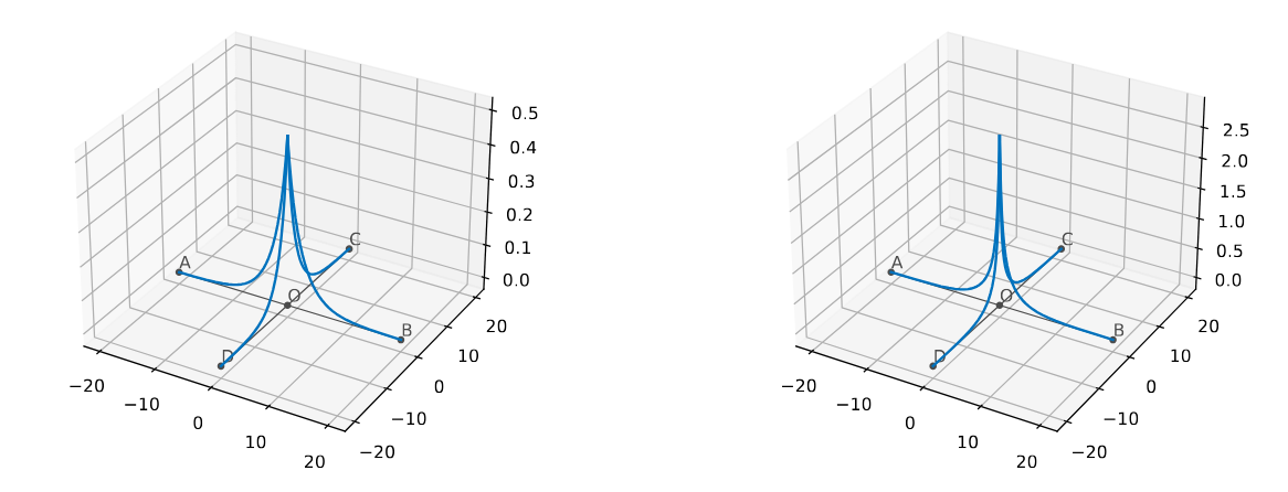
Figure 1. Action ground state for $\delta$-type condition (left) and $\delta^{\prime}$-type condition (right) for $p=3$, $K=4$, $\gamma=-2$, $\omega=1/8$.

We immediately deduce the following corollary from Lemma 4.1 and Theorem 1.1.

Corollary 4.3.

Let $p>1$, $\omega\in(0,-l_{\operatorname{H}_{i}})$, $\gamma<0$ and $i\in\{\delta,\delta^{\prime}\}$ be fixed. The set of action ground states on the star graph $\mathcal{G}$ is given by $\mathcal{A}_{\omega}=\{e^{i\theta}\phi_{\omega}:\theta\in[0,2\pi)\}$, where $\phi_{\omega}$ is given by (33), and is stable.

As it is unique up to phase shifts, we will now refer to $\phi_{\omega}$ given by (33) as the action ground state of $S_{\omega}$. We study the relation between the parameter $\omega$ and the mass of the action ground state for different values of $p$. The following proposition states that for $1<p<5$, the mass of the action ground state belongs to a finite interval, whereas for $p>5$, the mass of the action ground state belongs to $\mathbb{R}^{+}$.

Proposition 4.4.

Let $\omega\in(0,-l_{\operatorname{H}_{i}})$, $\gamma<0$ and $i\in\{\delta,\delta^{\prime}\}$ be fixed. The following properties hold:

1. For $1<p<5$, there exists $\mu=\mu(p)<\infty$ such that the function $\omega\in(0,-l_{\operatorname{H}_{i}})\mapsto M(\phi_{\omega})$ takes values in $(0,\mu)$ and is strictly decreasing.

2. For $p\geq 5$, the function $\omega\in(0,-l_{\operatorname{H}_{i}})\mapsto M(\phi_{\omega})$ takes values in $(0,\infty)$ and is strictly decreasing.

Proof.

Let be $i\in\{\delta,\delta^{\prime}\}$ be fixed. We first consider $p\in(1,\infty)\setminus\{5\}$. Applying the change of variable $y=(p-1)\sqrt{\omega}x/2+b_{\omega}$, we have

$$M(\phi_{\omega})=K\left(\frac{p+1}{2}\right)^{\frac{2}{p-1}}\omega^{\frac{5-p}{2(p-1)}}\int_{b_{\omega}}^{\infty}\sinh(y)^{-\frac{4}{p-1}}dy,$$

with

$$b_{\omega}\to\begin{cases}0\text{ as }\omega\to 0,\\ \infty\text{ as }\omega\to-l_{\operatorname{H}_{i}}.\end{cases}$$

We immediately have

(35) $$M(\phi_{\omega})\to 0\text{ as }\omega\to-l_{\operatorname{H}_{i}}$$

by dominated convergence theorem. We consider now the case where $\omega$ is asymptotically close to $0$. We separate the integral in two terms: an integral between $b_{\omega}$ and $b_{\omega}+1$, and an integral between $b_{\omega}+1$ and $\infty$. Observe that

$$\omega^{\frac{5-p}{2(p-1)}}\int_{b_{\omega}+1}^{\infty}\sinh(y)^{-\frac{4}{p-1}}dy\to 0\text{ as }\omega\to 0.$$

Furthermore, by Taylor expansion of $\sinh$, we have

$$\int_{b_{\omega}}^{b_{\omega}+1}(2\sinh(y))^{-\frac{4}{p-1}}dy=\int_{b_{\omega}}^{b_{\omega}+1}y^{-\frac{4}{p-1}}(1+\epsilon(y))^{-\frac{4}{p-1}}dy$$

where $\epsilon(y)=o_{y\to 0}(1)$. Furthermore, we have

(36) $$\int_{b_{\omega}}^{b_{\omega}+1}y^{-\frac{4}{p-1}}dy=C\left((b_{\omega}+1)^{\frac{p-5}{p-1}}-b_{\omega}^{\frac{p-5}{p-4}}\right),$$

where $C>0$. For $1<p<5$, the order of convergence of $M(\phi_{\omega})$ as $\omega\to 0$ is given by

$$\omega^{\frac{5-p}{2(p-1)}}b_{\omega}^{\frac{p-5}{p-4}}=\omega^{\frac{5-p}{2(p-1)}}\left(\omega^{\frac{p-5}{2(p-1)}}+o_{\omega\to 0}\left(\omega^{\frac{p-5}{2(p-1)}}\right)\right)=1+o_{\omega\to 0}(1)$$

by using (36), removing the term $(b_{\omega}+1)^{(p-5)/(p-1)}$ and doing a Taylor expansion of $b_{\omega}$. Thus, there exists $\mu>0$ such that

(37) $$M(\phi_{\omega})\to\mu\text{ as }\omega\to\infty.$$

For $p>5$, we have

$$\omega^{\frac{5-p}{2(p-1)}}(b_{\omega}+1)^{\frac{p-5}{p-1}}\to\infty\text{ as }\omega\to 0$$

so

(38) $$M(\phi_{\omega})\to\infty\text{ as }\omega\to 0.$$

As $\omega\mapsto M(\phi_{\omega})$ is injective and continuous by Remark 3.9, we obtain that it is strictly decreasing and taking values in $(0,\mu)$ if $p<5$ by (35)-(37), and on $(0,\infty)$ if $p>5$ by (35)-(38).

For $p=5$, we have

(39) $$M(\phi_{\omega}) =K\sqrt{3}\int_{b_{\omega}}^{\infty}\sinh(y)^{-1}dy=K\sqrt{3}\left(\ln(e^{b_{\omega}}+1)-\ln(e^{b_{\omega}}-1)\right)$$

$$=K\sqrt{3}\ln\left(\sqrt{-\frac{l_{\operatorname{H}_{i}}}{\omega}}\right).$$

We deduce from this explicit formulation all the the properties mentioned in the statement of the proposition, and this concludes the proof. ∎

Remark 4.5.

By (33), for $p=3$, we get on each edge $e\in\mathcal{E}$

$$\|\phi_{e}\|_{L^{2}{(\mathbb{R}^{+})}}^{2}=2\omega\int_{0}^{\infty}\sinh\left(\sqrt{\omega}x+b_{\omega}\right)^{-2}dx=2\sqrt{\omega}\left(\frac{1}{\tanh(b_{\omega})}-1\right)$$

By (34), we obtain

$$\|\phi_{e}\|_{L^{2}{(\mathbb{R}^{+})}}^{2}=2(\sqrt{-l_{\operatorname{H}_{i}}}-\sqrt{\omega}).$$

Consequently, for $|\mathcal{E}|=K$, we obtain

$$\|\phi_{\omega}\|_{L^{2}(\mathcal{G})}^{2}=K\|\phi_{e}\|_{L^{2}{(\mathbb{R}^{+})}}^{2}=2K\left(\frac{|\gamma|}{K}-\sqrt{\omega}\right)$$

for the $\delta$- coupling and, in the same way,

$$\|\phi_{\omega}\|_{L^{2}(\mathcal{G})}^{2}=2K\left(\frac{K}{|\gamma|}-\sqrt{\omega}\right)$$

for the $\delta^{\prime}$- coupling. Thus, for the $\delta$-coupling, the maximum mass allowed is $2|\gamma|$, and is independent on the number of edges. In contrast, for the $\delta^{\prime}$- coupling, the maximum mass is given by $2K^{2}/|\gamma|$, which increases as the number of the edges grows.

Furthermore, we explicitly computed the masses for $p=5$ for both $\delta$ and $\delta^{\prime}$ couplings in (39). Figure 2 illustrates the different behaviors for $p=3,5,7$, where $p=7$ is computed numerically.

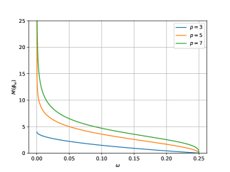
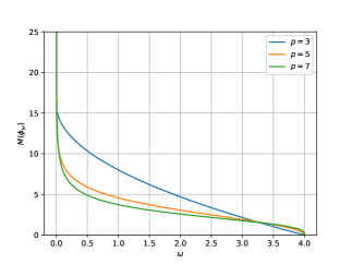
Figure 2. Mass of the ground state for $\delta$-type condition (left) and $\delta^{\prime}$-type condition (right) for $p=3,5,7$, $K=4$, $\gamma=-2$.

References

- [1] R. Adami, C. Cacciapuoti, D. Finco, and D. Noja. Constrained energy minimization and orbital stability for the NLS equation on a star graph. Ann. Inst. Henri Poincaré, Anal. Non Linéaire, 31(6):1289–1310, 2014.
- [2] R. Adami, C. Cacciapuoti, D. Finco, and D. Noja. Variational properties and orbital stability of standing waves for NLS equation on a star graph. J. Differ. Equations, 257(10):3738–3777, 2014.
- [3] R. Adami, D. Noja, and N. Visciglia. Constrained energy minimization and ground states for NLS with point defects. Discrete Contin. Dyn. Syst., Ser. B, 18(5):1155–1188, 2013.
- [4] R. Adami, E. Serra, and P. Tilli. NLS ground states on graphs. Calc. Var. Partial Differ. Equ., 54(1):743–761, 2015.
- [5] R. Adami, E. Serra, and P. Tilli. Negative energy ground states for the -critical NLSE on metric graphs. Commun. Math. Phys., 352(1):387–406, 2017.
- [6] G. P. Agrawal. Nonlinear fiber optics. In Nonlinear science at the dawn of the 21st century, pages 195–211. Berlin: Springer, 2000.
- [7] T. Akahori, Y. Bahri, S. Ibrahim, and H. Kikuchi. Pitchfork bifurcation at line solitons for nonlinear Schrödinger equations on the product space . Ann. Henri Poincaré, 25(7):3467–3497, 2024.
- [8] G. Berkolaiko and P. Kuchment. Introduction to quantum graphs, volume 186 of Mathematical Surveys and Monographs. American Mathematical Society, Providence, RI, 2013.
- [9] C. Besse, R. Duboscq, and S. Le Coz. Numerical Simulations on Nonlinear Quantum Graphs with the GraFiDi Library. The SMAI Journal of computational mathematics, 8:1–47, 2022.
- [10] G. Bianconi and A.-L. Barabási. Bose-einstein condensation in complex networks. Phys. Rev. Lett., 86:5632–5635, Jun 2001.
- [11] F. Boni and R. Carlone. NLS ground states on the half-line with point interactions. NoDEA, Nonlinear Differ. Equ. Appl., 30(4):23, 2023. Id/No 51.
- [12] I. Brunelli, G. Giusiano, F. P. Mancini, P. Sodano, and A. Trombettoni. Topology-induced spatial bose–einstein condensation for bosons on star-shaped optical networks. Journal of Physics B: Atomic, Molecular and Optical Physics, 37(7):S275, 2004.
- [13] R. Burioni, D. Cassi, M. Rasetti, P. Sodano, and A. Vezzani. Bose-einstein condensation on inhomogeneous complex networks. Journal of Physics B: Atomic, Molecular and Optical Physics, 34(23):4697, 2001.
- [14] T. Cazenave. Semilinear Schrödinger equations, volume 10 of Courant Lecture Notes in Mathematics. New York University / Courant Institute of Mathematical Sciences, New York, 2003.
- [15] T. Cazenave and P.-L. Lions. Orbital stability of standing waves for some nonlinear Schrödinger equations. Commun. Math. Phys., 85:549–561, 1982.
- [16] C. De Coster, S. Dovetta, D. Galant, and E. Serra. On the notion of ground state for nonlinear Schrödinger equations on metric graphs. Calc. Var. Partial Differ. Equ., 62(5):28, 2023. Id/No 159.
- [17] C. De Coster, S. Dovetta, D. Galant, E. Serra, and C. Troestler. Constant sign and sign changing nls ground states on noncompact metric graphs. Preprint, arXiv: 2306.12121[math.AP] (2023), 2023.
- [18] A. de Laire, P. Gravejat, and D. Smets. Minimizing travelling waves for the Gross-Pitaevskii equation on . Annales de la Faculté des Sciences de Toulouse. Mathématiques., to appear, 2024.
- [19] S. Dovetta, E. Serra, and P. Tilli. Action versus energy ground states in nonlinear Schrödinger equations. Math. Ann., 385(3-4):1545–1576, 2023.
- [20] D. Edmunds and D. Evans. Spectral theory and differential operators. Oxford: Oxford University Press, 2nd revised edition edition, 2018.
- [21] R. Fukuizumi and L. Jeanjean. Stability of standing waves for a nonlinear Schrodinger equation with a repulsive Dirac delta potential. Discrete and Continuous Dynamical Systems, 21(1):121, 2008.
- [22] R. Fukuizumi, M. Ohta, and T. Ozawa. Nonlinear schrödinger equation with a point defect. In Annales de l’Institut Henri Poincaré C, Analyse non linéaire, volume 25,5, pages 837–845. Elsevier, 2008.
- [23] E. Gagliardo. Ulteriori proprieta di alcune classi di funzioni in piu variabili. Ric. Mat., 8:24–51, 1959.
- [24] R. H. Goodman, P. J. Holmes, and M. I. Weinstein. Strong NLS soliton–defect interactions. Phys. D: Nonlinear Phenomena, 192(3-4):215–248, 2004.
- [25] A. Grecu and L. I. Ignat. The Schrödinger equation on a star-shaped graph under general coupling conditions. J. Phys. A, Math. Theor., 52(3):26, 2019. Id/No 035202.
- [26] S. Gustafson, S. Le Coz, and T.-P. Tsai. Stability of periodic waves of 1d cubic nonlinear Schrödinger equations. AMRX, Appl. Math. Res. Express, 2017(2):431–487, 2017.
- [27] L. Jeanjean and S.-S. Lu. On global minimizers for a mass-constrained problem. Calc. Var. Partial Differ. Equ., 61(6):18, 2022.
- [28] A. Kairzhan, D. Noja, and D. E. Pelinovsky. Standing waves on quantum graphs. J. Phys. A, Math. Theor., 55(24):51, 2022. Id/No 243001.
- [29] M. Kaminaga and M. Ohta. Stability of standing waves for nonlinear Schrödinger equation with attractive delta potential and repulsive nonlinearity. Saitama Math. J., 26:39–48, 2009.
- [30] V. Kostrykin and R. Schrader. Laplacians on metric graphs: eigenvalues, resolvents and semigroups. In Quantum graphs and their applications. Proceedings of an AMS-IMS-SIAM joint summer research conference on quantum graphs and their applications, Snowbird, UT, USA, June 19–23, 2005, pages 201–225. Providence, RI: American Mathematical Society (AMS), 2006.
- [31] S. Kosugi. A semilinear elliptic equation in a thin network-shaped domain. Journal of the Mathematical Society of Japan, 52(3):673–697, 2000.
- [32] S. Kosugi. Semilinear elliptic equations on thin network-shaped domains with variable thickness. J. Differ. Equations, 183(1):165–188, 2002.
- [33] S. Le Coz, R. Fukuizumi, G. Fibich, B. Ksherim, and Y. Sivan. Instability of bound states of a nonlinear Schrödinger equation with a Dirac potential. Phys. D, 237(8):1103–1128, 2008.
- [34] S. Le Coz and B. Shakarov. Ground states on a fractured strip and one dimensional reduction. Preprint, arXiv:2411.18187 [math.AP] (2024), 2024.
- [35] G. Leo and G. Assanto. Multiple branching of vectorial spatial solitary waves in quadratic media. Optics communications, 146(1-6):356–362, 1998.
- [36] J. L. Lions and E. Magenes. Non-homogeneous boundary value problems and applications. Vol. I. Translated from the French by P. Kenneth, volume 181 of Grundlehren Math. Wiss. Springer, Cham, 1972.
- [37] P.-L. Lions. The concentration-compactness principle in the calculus of variations. The limit case. I. Rev. Mat. Iberoam., 1(1):145–201, 1985.
- [38] M. Mariş and A. Mur. Periodic traveling waves for nonlinear schrödinger equations with non-zero conditions at infinity in . Preprint, arXiv:2404.11772 [math.AP] (2024), 2024.
- [39] L. Nirenberg. On elliptic partial differential equations. Ann. Sc. Norm. Super. Pisa, Sci. Fis. Mat., III. Ser., 13:115–162, 1959.
- [40] J. A. Pava and N. Goloshchapova. On the orbital instability of excited states for the NLS equation with the -interaction on a star graph. Discrete Contin. Dyn. Syst., 38(10):5039–5066, 2018.
- [41] L. Pitaevskii and S. Stringari. Bose-Einstein condensation and superfluidity, volume 164 of Int. Ser. Monogr. Phys. Oxford: Oxford University Press, 2016.
- [42] S. Terracini, N. Tzvetkov, and N. Visciglia. The nonlinear Schrödinger equation ground states on product spaces. Analysis & PDE, 7(1):73–96, 2014.
- [43] G. Teschl. Mathematical methods in quantum mechanics, volume 157. American Mathematical Soc., 2014.
- [44] Y. Yamazaki. Transverse instability for a system of nonlinear Schrödinger equations. Discrete Contin. Dyn. Syst., Ser. B, 19(2):565–588, 2014.
- [45] Y. Yamazaki. Stability of line standing waves near the bifurcation point for nonlinear Schrödinger equations. Kodai Math. J., 38(1):65–96, 2015.