Radon–Nikodým Derivative: Re-imagining Anomaly Detection from a Measure Theoretic Perspective

Abstract

Which principle underpins the design of an effective anomaly detection loss function? The answer lies in the concept of Radon–Nikodým theorem, a fundamental concept in measure theory. The key insight is – Multiplying the vanilla loss function with the Radon–Nikodým derivative improves the performance across the board. We refer to this as RN-Loss.

This is established using PAC learnability of anomaly detection. We further show that the Radon–Nikodým derivative offers important insights into unsupervised clustering based anomaly detections as well.

We evaluate our algorithm on 96 datasets, including univariate and multivariate data from diverse domains, including healthcare, cybersecurity, and finance. We show that RN-Derivative algorithms outperform state-of-the-art methods on 68% of Multivariate datasets (based on F-1 scores) and also achieves peak F1-scores on 72% of time series (Univariate) datasets.

1 Introduction

Anomaly detection, the process of identifying rare yet significant deviations from normal patterns, has become essential in various domains such as finance, healthcare, and cybersecurity, where undetected anomalies can lead to catastrophic consequences. Researchers have explored supervised and unsupervised approaches for anomaly detection. Although unsupervised approaches work well when labeled anomalies are scarce and often not found in training data, shallow unsupervised anomaly detection methods like One-Class SVM Manevitz and Yousef [2002], Isolation Forest Liu et al. [2008] are limited in their scalability to large datasets Ruff et al. [2020]. Tree-based algorithms such as Isolation Forest, Random Cut Forest Guha et al. [2016], d-BTAI Sarkar et al. [2021b], and MGBTAI Sarkar et al. [2023], report a comparatively better performance. Supervised learning needs to use labeled data and has difficulty identifying unseen anomaliesKawachi et al. [2018],Chandola et al. [2009]; it also offers several advantages that make them a favorable choice. For example, supervised algorithms can leverage domain knowledge to recognize complex patterns indicative of anomalies by training on labeled examples of both normal and anomalous instances. This results in improved accuracy and precision compared to unsupervised methods, which rely on more generalized patterns and assumptions Görnitz et al. [2012], Ruff et al. [2020]. Supervised algorithms suffer from the class imbalance issue because loss functions used in these algorithms assume equally distributed datasets across multiple classes.

Motivation of the present work:

Anomaly detection has been a long-standing focus of research, addressing diverse applications such as fraud detection, network security, and medical diagnostics Chandola et al. [2009], Hilal et al. [2022], Bhattacharyya and Kalita [2013]. Numerous approaches have achieved state-of-the-art performance, supported by robust empirical studies Shen et al. [2020b], Hojjati et al. [2024]. However, to the best of our knowledge, no prior work has derived a generic principle for designing the loss function leaving a critical gap in the theoretical understanding of anomaly detection. This work aims to bridge this gap by deriving such a loss function and providing foundational insights into its properties and implications for anomaly detection tasks.

Significant efforts have been devoted to the principled study of the related problem of out-of-distribution (OOD) detection, as detailed in prior work (See Fang et al. [2024] and references therein). While these studies provide valuable insights, OOD detection fundamentally differs in it’s objectives and assumptions compared to anomaly detection. Specifically, OOD detection focuses on identifying inputs not represented by the training data distribution, whereas anomaly detection typically involves identifying rare or unexpected patterns within the data itself (See Salehi et al. [2022] for comparison). For a comprehensive review of the literature addressing both paradigms, please refer to Appendix E.

Contributions/Insights

The key contribution of this paper is the rethinking of anomaly detection from first principles (PAC learnability) and the introduction of a weighted loss function based on the Radon–Nikodým derivative (termed “RN-Loss” in this paper), tailored for anomaly detection.

Theoretical Insights:

In Section 2 we introduce the problem of (PAC-)learnability of anomaly detection problem. In Section 3 we show that anomaly detection is indeed learnable under some mild conditions (see informal summary) of (PAC-)learnability. The main insight from this derivation is – The generic loss function for learning anomaly detection is the product of the original loss function and the Radon–Nikodým derivative of the two respective distributions. An operator (Radon–Nikodým derivative) is able to calibrate the two different measures i.e. distributions. This enables identifying anomalies in the data distribution. Further we also show that, this divergence in distributions can be quantified using the anomaly contamination ratio. This interpretation and formal proof also turned out to be performant when tested on diverse datasets. Specifically, if one has samples and used the empirical estimate, then the ideal (generic) loss function tailored for anomaly detection becomes a (appropriately) weighted loss. In other cases (unsupervised), it reduces to the ratio of kernel density estimates.

Empirical Insights:

RN-Loss maintains computational efficiency by building on base loss functions like Binary Cross-Entropy, enabling integration with architectures such as Feedforward ReLU and LSTM models. Further unsupervised methods like dBTAI Sarkar et al. [2021b] can benefit from an adapted version of RN-Loss thus making it capable of identifying anomalies even when the model is trained solely on normal data. This ability to detect previously unseen anomalies demonstrates its robustness and effectiveness in scenarios where anomalous data is not present during training. It supports operational simplicity with automated hyperparameter tuning via AUC ROC, removing the need for manual thresholding (Appendix F, Table 15).

The loss function demonstrates flexibility, fitting varied data distributions such as Weibull and Log-normal without requiring structural changes (Appendix F, Table 13). These properties make RN-Loss a robust and adaptable approach for anomaly detection, combining improved metrics, efficiency, and versatility, making it suitable for diverse applications in real-world scenarios.

Consequences:

The RN-Loss function introduces improvements in anomaly detection, achieving enhanced performance and broad adaptability. It outperforms prior SoTA methods, improving F-1 Scores in 68% and Recall in 46% of the multivariate datasets, with similar trends in time-series (Univariate) data (F-1: 72%, Recall: 83%). These results demonstrate its consistent performance across diverse benchmarks.
Our experiments demonstrate that RN-Loss significantly improves the performance of unsupervised anomaly detection methods, specifically vanilla implementation of CBLOF and ECBLOF Sarkar et al. [2021a], when combined with clustering algorithms like K-Means Gao [2009] and dBTAI Sarkar et al. [2021b]. The enhanced KMeans-CBLOF algorithm achieved superior performance on 93% of univariate datasets (27 out of 29) and 48% of multivariate datasets (32 out of 67) in comparison to the original KMeans-CBLOF algorithm. While dBTAI previously achieved state-of-the-art results, its metrics—particularly precision—were inflated. RN-Loss helped normalize these metrics and the modified dBTAI further maintained or improved its overall performance across 59 multivariate datasets and demonstrated increased recall values across nearly all univariate datasets. Detailed experimental results are presented in Table 41, Table 42, Table 43 and Table 44 in the Appendix F. For the mathematical foundations of adapting CBLOF and ECBLOF to RN-Loss, please refer to Appendices Appendix C and Appendix D, respectively.

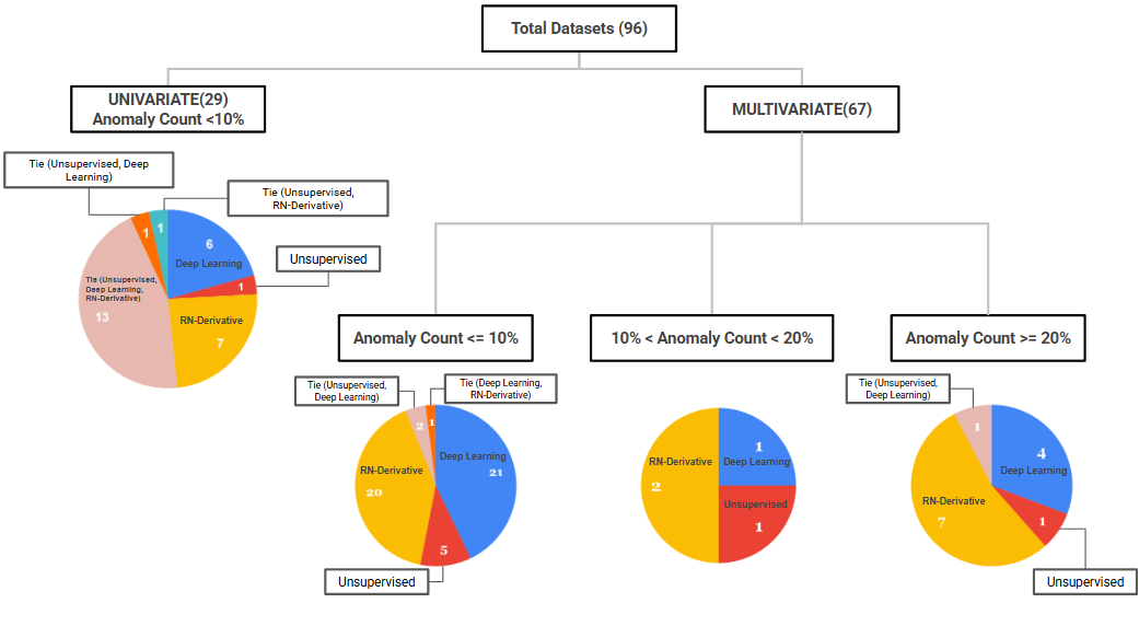
Figure 1: Comparative Analysis of Anomaly Detection Algorithms. Performance evaluation prioritizes recall, with precision as the secondary metric for tied cases. The comparison spans three algorithm categories: (1) Deep Learning approaches (AutoEncoders, DAGMM, DevNet, GAN, DeepSAD, FTTransformer (current state-of-the-art), and PReNet), (2) Unsupervised methods (LOF, Elliptic Envelope, Isolation Forest, dBTAI, MGBTAI, and quantile-based approaches including q-LSTM variants and QReg), and (3) RN-Derivative algorithms (RN-Net and RN-LSTM). RN-Net outperforms state-of-the-art methods on 68% of Multivariate datasets (based on F-1 scores), while the RN-LSTM + RN-Net combination achieves peak F1-scores on 72% of time series (Univariate) datasets. For detailed numerical comparisons, refer to Tables 2, 3, 3 and 3 in Appendix F.

2 Problem Setup and Notation

Let ${\mathcal{X}}\subset\mathbb{R}^{d}$ denote the feature space and ${\mathcal{Y}}\in\{1,\dots,K\}$ denote the label space. The base distribution is denoted by a joint distribution $D_{X_{B}Y_{B}}$ over ${\mathcal{X}}\times{\mathcal{Y}}$, where $X_{B}\in{\mathcal{X}}$ and $Y_{B}\in{\mathcal{Y}}$. The anomaly distribution is denoted by $D_{X_{A}Y_{A}}$ over the same ${\mathcal{X}}\times{\mathcal{Y}}$ and $X_{A}\in{\mathcal{X}}$. However, $Y_{A}$ does not belong to ${\mathcal{Y}}$ for simplicity we assume $Y_{A}=K+1$. We also often use the mapping $\phi$ which is a function which maps the labels $\{1,\dots,K\}\to 0$ and label $\{K+1\}\to 1$.

We assume that the distribution we sample from is a mixture of the base-distribution and the anomaly distribution, i.e $D_{XY}^{\alpha}=(1-\alpha)D_{X_{B}Y_{B}}+\alpha D_{X_{A}Y_{A}}$ where $\alpha\in[0,1)$ is unknown. $\alpha$ is referred to as anomaly contamination ratio. We sometimes omit the $\alpha$ when we imply that $\alpha$ can be any unknown value.

Anomaly detection can either be supervised and unsupervised. For completeness, we state both these problems below.

Supervised Anomaly Detection:

Given a sample of points $S\coloneqq\{({\bm{x}}^{i},y^{i})\}$ drawn i.i.d from $D_{XY}$, the aim is to obtain a classifier $f$ such that, for any sample ${\bm{x}}$ from marginal $D_{X}$ : (i) if ${\bm{x}}$ is sampled from $D_{X_{A}}$ then identify it as anomaly and (ii) if ${\bm{x}}$ is sampled from $D_{X_{B}}$ identify it as non-anomaly. Note that we have at our disposal the labels – $\phi\circ{\mathcal{Y}}\in\{0,1\}$, making this a binary classification problem.

Unsupervised Anomaly Detection:

Given a sample of points $S\coloneqq\{({\bm{x}}^{i},y^{i})\}$ drawn i.i.d from $D_{X_{B}Y_{B}}$, the aim is to obtain a classifier $f$ such that, for any sample ${\bm{x}}$ from marginal $D_{X}$ : (i) if ${\bm{x}}$ is sampled from $D_{X_{A}}$ then identify it as anomaly and (ii) if ${\bm{x}}$ is sampled from $D_{X_{B}}$ identify it as non-anomaly.

Remark:

Supervised and unsupervised cases differ by the sampling distribution $D_{XY}$ vs $D_{X_{B}Y_{B}}$ and whether we have “some” labels to identify the classifier $f$.

Space of Distributions:

Clearly, if there is no restriction on the set of possible distributions $D_{XY}$, no-free-lunch theorem Wolpert [1996] suggests that anomaly detection is impossible. So, we restrict the set of distributions to a set $\mathscr{D}_{XY}$.

Hypothesis Space, Loss function and Risks :

Let ${\mathcal{H}}\subset\{h:{\mathcal{X}}\to\{0,1\}\}$ denote the set of functions from which we choose our classifier $f$. Any specific $h\in{\mathcal{H}}$ is referred to as hypothesis function or simply function if the context is clear. We consider 0-1 loss function – $\ell:{\mathcal{Y}}\times{\mathcal{Y}}\to\{0,1\}$ where $\ell(y_{1},y_{2})=0$ if $y_{1}=y_{2}$ and $\ell(y_{1},y_{2})=1$ otherwise.

The risk of a hypothesis is defined as the expected loss when the hypothesis is used for identifying anomalies.

$$R_{D}(h)=E_{D_{XY}}[\ell(h({\bm{x}}),y)]$$ (1)

We also define $\alpha-$risk to quantify the expected loss when anomaly contamination ratio is $\alpha\in[0,1)$. That is, $D=(1-\alpha)D_{X_{B}Y_{B}}+\alpha D_{X_{A}Y_{A}}$

$$R_{D}^{\alpha}(h)=(1-\alpha)R_{D_{X_{B}Y_{B}}}(h)+\alpha R_{D_{X_{A}Y_{A}}}(h)$$ (2)

PAC Learning and Anomaly Detection:

We use the following equivalent definition of PAC learning Ratsaby [2008] in this article. A hypothesis class ${\mathcal{H}}$ is (agnostic-)PAC learnable if there exists (i) an algorithm $\mathbf{A}:\cup_{n=1}^{\infty}({\mathcal{X}}\times{\mathcal{Y}})^{n}\to{\mathcal{H}}$, (ii) a decreasing sequence $\epsilon(n)\to 0$, and (iii) for all $D_{XY}\in\mathscr{D}_{XY}$

$$E_{S\sim D_{XY}^{n}}[R_{D_{XY}}(\mathbf{A}(S))-\inf_{h\in{\mathcal{H}}}R_{D_{XY}}(h)]\leq\epsilon(n)$$ (3)

Existing results Vapnik and Chervonenkis [1971] show that if ${\mathcal{H}}$ has finite VC dimension, then it is learnable for all possible distributions $\mathscr{D}_{XY}$. Specifically, neural networks are PAC learnable.

Note that we are interested in the anomaly detection. Which means, while learning may be done with specific $\alpha$, the test distribution is always fixed at $\alpha=0.5$. Formally, we sample from $D_{XY}^{\alpha}$, but the risk we are interested is when base-distribution and anomalies are equally possible, i.e $\alpha=0.5$. Thus, we need to show that

$$E_{S\sim D_{XY}^{\alpha,n}}[R_{D_{XY}}^{0.5}(\mathbf{A}(S))-\inf_{h\in{\mathcal{H}}}R_{D_{XY}}^{0.5}(h)]\leq\epsilon(n)\\$$ (4)

where $\epsilon(n)\to 0$ as $n\to\infty$.

3 RNLoss : Derivation from first principles

The aim of this article is to obtain the algorithm $\mathbf{A}$ for solving the anomaly detection problem. We achieve this in 2 stages - (i) Assume that $\alpha$ is known and design a loss using the Radon–Nikodým(RN) derivative, (ii) Design the loss function which approximates $\alpha$.

We begin by recalling the established Radon–Nikodým theorem from measure theory.

Theorem 3.1 (Radon–Nikodým Konstantopoulos et al. [2011]).

Let $(\Omega,\mathcal{A})$ be a measurable space with $\mathcal{A}$ as the $\sigma$ algebra and $\mu,\nu$ denote two $\sigma-$finite measures such that $\nu<<\mu$ ($\nu$ is absolutely continuous with respect to $\mu$). Then, there exists a function $f$ such that,

$$\nu(A)=\int_{A}fd\mu\quad(or)\quad d\nu=fd\mu$$ (5)

where A $\in\mathcal{A}$.

Absolute Continuity and bounded Assumption:

For any fixed $\alpha$, let $\nu$ denote the measure induced by $D_{XY}^{0.5}$ and $\mu$ denote the measure induced by $D_{XY}^{\alpha}$. We assume that $\nu$ is absolutely continuous with respect to $\mu$. We further assume that the density $f$ relating these distributions is bounded, i.e $1/b<f<b$ for some $b$ on the support of $\mu$.

We then have the following theorem:

Theorem 3.2.

Let $\nu$ denote the measure induced by $D_{XY}^{0.5}$ and $\mu$ denote the measure induced by $D_{XY}^{\alpha}$. Also, let $d\nu=fd\mu$ (absolutely continuous) where $1/b<f<b$ for some $b<\infty$ on the support of $\mu$. For all $h\in{\mathcal{H}}$, there exists a $\Delta_{\mu,\nu}$ such that,

$$\frac{1}{\Delta_{\mu,\nu}}\leq\frac{R_{D_{XY}^{0.5}}(h)}{R_{D_{XY}^{\alpha}}(h)}\leq\Delta_{\mu,\nu}$$ (6)

The proof is given in Appendix A.

Using Theorem 3.2, we have

$$R_{D_{XY}^{0.5}}(\mathbf{A}(S))\leq R_{D_{XY}^{\alpha}}(\mathbf{A}(S))\times\Delta_{\mu,\nu}$$ (7)

and,

$$\inf_{h\in{\mathcal{H}}}R_{D_{XY}^{0.5}}(h)\geq\frac{1}{\Delta_{\mu,\nu}}\inf_{h\in{\mathcal{H}}}R_{D_{XY}^{\alpha}}(h)$$ (8)

Hence,

$$R_{D_{XY}^{0.5}}(\mathbf{A}(S))-\inf_{h\in{\mathcal{H}}}R_{D_{XY}^{0.5}}(h)$$ (9)

$$\leq R_{D_{XY}^{\alpha}}(\mathbf{A}(S))\times\Delta_{\mu,\nu}-\frac{1}{\Delta_{\mu,\nu}}\inf_{h\in{\mathcal{H}}}R_{D_{XY}^{\alpha}}(h)$$

$$\leq\Delta_{\mu,\nu}\left[R_{D_{XY}^{\alpha}}(\mathbf{A}(S))-\inf_{h\in{\mathcal{H}}}R_{D_{XY}^{\alpha}}(h)\right]$$

$$+\inf_{h\in{\mathcal{H}}}R_{D_{XY}^{\alpha}}(h)\left[-\frac{1}{\Delta_{\mu,\nu}}+\Delta_{\mu,\nu}\right]$$

Taking expectations on both sides,

$$E_{S\sim D_{XY}^{\alpha,n}}[R_{D_{XY}^{0.5}}(\mathbf{A}(S))-\inf_{h\in{\mathcal{H}}}R_{D_{XY}^{0.5}}(h)]$$ (10)

$$\leq\Delta_{\mu,\nu}E_{S\sim D_{XY}^{\alpha,n}}[R_{D_{XY}^{\alpha}}(\mathbf{A}(S))-\inf_{h\in{\mathcal{H}}}R_{D_{XY}^{\alpha}}(h)]$$

$$+\left[-\frac{1}{\Delta_{\mu,\nu}}+\Delta_{\mu,\nu}\right]E_{S\sim D_{XY}^{\alpha,n}}\left[\inf_{h\in{\mathcal{H}}}R_{D_{XY}^{\alpha}}(h)\right]$$

Using the Realizability Assumption of the PAC learning framework, we have that

$$E_{S\sim D_{XY}^{\alpha,n}}\left[\inf_{h\in{\mathcal{H}}}R_{D_{XY}^{\alpha}}(h)\right]=0.$$ (11)

Assuming that ${\mathcal{H}}$ is PAC learnable, we have that

$$E_{S\sim D_{XY}^{\alpha,n}}[R_{D_{XY}^{0.5}}(\mathbf{A}(S))-\inf_{h\in{\mathcal{H}}}R_{D_{XY}^{0.5}}(h)]\leq\epsilon(n)$$ (12)

where $\epsilon(n)\to 0$ as $n\to\infty$.

Summary (informal):

To summarize, if $\alpha$ is known, the distribution space $\mathscr{D}_{XY}$ is such that (i) absolute continuity holds, (ii) relation between the measures is bounded, and if the ${\mathcal{H}}$ is such that realizability assumption holds then the anomaly detection problem is learnable.

Estimating empirical distribution function of $f$ to get the loss function:

It is easy to see that, if $\alpha$ is known the loss function to be minimized is $\ell(h(x),y)f(x)$, where $f$ is the RN derivative above. (See proof in Appendix A for details). So, in the supervised case we can estimate $f\approx\hat{f}$ using the empirical distribution function.

If we let the weight of the anomalous class $D_{X_{A}Y_{A}}$ to be $1$, then the samples from the majority class $D_{X_{B}Y_{B}}$ are reweighted by

$$\omega=\frac{\alpha}{1-\alpha}\approx\frac{\#\text{samples in Minority}}{\#\text{samples in Majority}}$$ (13)

In the experiments we use $\omega$ as tuning hyper-parameter to the loss. See Appendix B for detailed derivation.

Important Remarks:

• Note that the assumptions made in the above section are reasonable for any practical situation. This is evidenced by the experiments in Section 4, where we validate the loss in a variety of settings.

• Note that the loss function $\ell(.,.)$ can be supervised/unsupervised. The RN-Loss is a generic loss function which mandates multiplying the base loss function with the Radon–Nikodým derivative. One can in theory use any suitable approximation to $f$. However, as we see in Section 4, Equation 13 works well when the relevant information is available.

• Generalization: The RN-Loss can be easily adapted to the unsupervised anomaly detection framework, as demonstrated in the CBLOF and ECBLOF examples. The key insight is addressing the discrepancy between the empirical imbalanced distribution ($D_{XY}^{\alpha}$ - with cluster size bias) and the desired balanced distribution ($D_{XY}^{0.5}$). In clustering-based anomaly detection methods, the data is assumed to come from a mixture of distributions, where each cluster represents a component. The RN-Loss framework corrects the inherent bias introduced by cluster sizes by applying a derivative function that accounts for the density ratio between these distributions. For instance, in CBLOF, this correction leads to an adjusted anomaly score that incorporates both the distance-based rarity and the cluster size, while in ECBLOF, it helps justify the removal of cluster size scaling to achieve unbiased detection. Detailed mathematical proofs can be found in Appendix C and Appendix D.

4 Experiments - Anomaly Detection

Datasets:

A total of 96 datasets (29 Univariate and 67 Multivariate) with anomalous instances in varying degrees were considered for evaluation from AD-Bench, SWaT, etc., with the notable inclusion of ESA-ADB, a recently published time series data set (Appendix F, Table 17). Our datasets cover multiple domains such as finance, healthcare, e-commerce, industrial systems, telecommunications, astronautics, computer vision, forensics, botany, sociology, linguistics, etc. The data volume ranges from 80 to 61,936, and the anomaly percentages range from 0.03% to 43.51%. We further split the datasets over three anomaly contamination ranges: i) less than 1% (critically imbalanced datasets), ii) between 1% to 10%, and iii) greater than 10% (moderately imbalanced datasets).

• Anomaly $<1$%: In this, we primarily focus on detecting extreme outliers or rare events as they deviate significantly from the normal, also being highly indicative of critical issues such as fraud or system failures. This set consists of 22 univariate and 4 multivariate datasets from different distributions such as Weibull and log-normal other than Gaussian.(Appendix F, Table 13)

• Anomaly between $1-10$%: This set also indicates outliers that are less frequent than the normal data but occur often enough to be noticeable. It consists of 47 datasets (40 multivariate and 7 univariate) with distributions such as Exponential, Weibull, Gamma, and Log-normal. Extensive research has been performed on these datasets over the past few years and is simultaneously documented in the form of surveys compiling all the methodologies presented to date, Samariya and Thakkar [2023], Cao et al. [2024].

• Anomaly $>10$%: These datasets comprise clusters of sample points that lie away from the general distribution and are termed outliers, such as in some cases of collective anomalies or contextual anomaly groups. This set has 16 multivariate datasets, including time series, with various domains covered in the Appendix.

A separate subsection of analysis has been done targeting Time Series anomaly detection in particular, where we use 29 univariate time-dependent and 7 multivariate time-dependent datasets, along with the newly proposed ESA-ADB dataset Kotowski et al. [2024] along with six other SWaT datasets Wang et al. [2019] and a BATADAL dataset.

Network Architecture:

We used two architecture in our study. First, RN-Net is a ReLU feedforward network with RN-Loss, comprising 64 hidden units in a binary classification setting. We train for 50 epochs using the Adam optimizer. Additionally, we use batch normalization Ioffe and Szegedy [2015], dropout Srivastava et al. [2014], and early stopping with a threshold of 10 epochs. We reduce our learning rate by half every 5 epochs until it reaches $10^{-6}$. Parallel to this, we integrated L2 regularisation with RN-Net and noticed a further step-up in performance across datasets (Results are in Appendix F, Tables 37 and 38).

Similarly, to demonstrate the flexibility and adaptability of RN-Loss, we create RN-LSTM: A LSTM with 32 hidden units coupled with the RN-Loss function.

Evaluation:

We adopt a modified approach to the traditional 70-30 data splitting technique. We allocate 70% of the normal data for training, while only 15% of the anomalous data is used for training. The remaining data, comprising 30% of the normal data and 85% of the anomalous data, is reserved for testing. This strategy is designed to evaluate the robustness of the model, particularly given that anomalies typically constitute less than 10% of the dataset. By using only 15% of these rare anomalies for training, the exposure to anomalous content is zero or minimal, encasing both scenarios of the model being trained on a completely normal dataset or with some anomaly contamination. The results from both setups are identical, which further eliminates the need for training on anomalous data, as in most supervised learning algorithms for optimal performance, like DevNet Gan et al. [2015], DAGMM Zong et al. [2018], etc.

Model-specific Threshold Tuning:

In the domain of anomaly detection, determining optimal threshold values is crucial due to the inherently rare and imbalanced nature of anomalies. Setting the threshold too low may lead to a high number of false positives, reducing the model’s significance, and setting it too high may cause the model to miss critical anomalies, which could be disastrous in fields like cybersecurity, fraud detection, etc. Therefore, aiming at the most optimal model performance, we set the following thresholds in accordance with the suggestions from the literature: For Autoencoders, the lower threshold is set at the $0.75$th percentile, and the upper threshold is at the $99.25$th percentile of Mean Squared Error(MSE) values. All the data points with discriminator scores less than $10$th percentile were considered anomalies for GANs. DAGMM had a dual threshold setting with high and low thresholds, with two standard deviations above and below the mean. For the tree-based approaches, MGBTAI was set to a minimum clustering threshold of 20% of the dataset size and leaf level threshold of 4, while for d-BTAI, the minimum clustering threshold was set to 10% of the dataset size. For deep quantile regression, the lower threshold was at $0.9$th percentile and the upper at $99.1$st percentile of the predicted values. The above settings help us in achieving State-of-The-Art results over the AD-Bench and Time series datasets, however, as observed this process becomes extremely meticulous and takes up most of the experimental time. Hence, for RN-NET and RN-LSTM, we automate our threshold calculation process by maximizing the difference in True positive and False positive rates, which are very important metrics obtained from the AUC-ROC curve. This helps us get the best optimal threshold, and SoTA results across datasets and overall algorithms. The thresholds range from 0.001 to 0.999 and can be found for all the respective datasets in Appendix F, Table 15.

Statistical Tests:

Each experiment was performed 5 times, after which mean and standard deviations for the repeats were calculated. We use Cohen’s $d$ effect size test, with the “medium” effect size popularized by Sawilowsky [2009] to declare wins, ties, and losses. A detailed comparison can be observed in Table 2 (Appendix F).

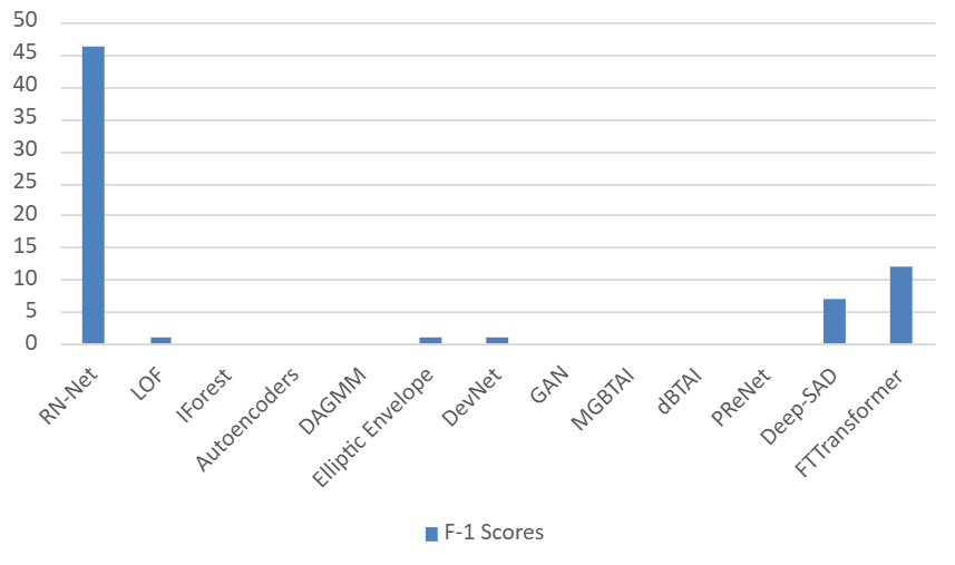
(a) F1 Scores of algorithms on 60 Multivariate Datasets

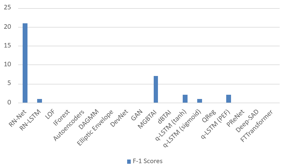
(b) F1 Scores of algorithms on 29 Univariate datasets

Figure 2: Comparison of algorithm performance on different datasets based on F1 Scores for 60 Multivariate and 29 Univariate Time Series datasets.(Excluding 7 Multivariate Datasets and ESA-ADB dataset). For other metrics (Precision, Recall and AUC-ROC) refer Figure 3 in Appendix F.

Baselines and SoTA:

The current SoTA algorithms used for comparison include Local Outlier Factor(LOF), Isolation Forest (IForest), One-class SVM (OCSVM), Autoencoders (IEEE TSMC, 2022) Deep Autoencoding Gaussian Mixture Model (DAGMM, ICLR, 2018), Quantile LSTM(q-LSTM, TAI, 2024), Deep Quantile Regression Tambuwal and Neagu [2021], GNN Deng and Hooi [2021](AAAI, 2021), GAN (NeurIps, 2020), DevNet(CVPR, 2015), MGBTAI and d-BTAI (2023) as covered in Table 4 in Appendix F. Above is a mix of supervised and unsupervised methods, forming our baselines for comparison on anomalous datasets. Some observations on the above algorithms are as follows: GAN performed well and achieved perfect recall on 14 datasets overall, however it classified all datapoints as anomalies in 13 datasets (including 6 SWaT datasets). This observation stemmed from the uniform discriminator score equal to 1, i.e. the algorithm classified all data points as anomalous. Deng and Hooi [2021] proposed an approach based on GNN (GDN) to detect anomalies in multivariate time series datasets. GDN, being a SoTA algorithm in this field, offers competition to RN-Net and RN-LSTM but still lags behind, as seen from table 39. Some datasets have more than 10% anomalies and hence make more of a classification problem rather than an anomaly detection problem, so a Linear SVM is used to quantify its performance and compared with RN-Net (Appendix F, Table 18). Further, to study univariate datasets in particular, we have included 4 quantile-based algorithms, 3 qLSTM with sigmoid, PEF, and tanh activation functions, and a deep quantile regression algorithm (Appendix F, Tables 9, 10, 11 and 12). Other important algorithms that have been tested along with the above are ECOD Li et al. [2023], COPOD Li et al. [2020], KNN, LUNAR Bergman and Hoshen [2020], PCA, DSVDD (Appendix F, Tables 27, 28, 29, 30, 31, 32, 33 and 34).

Dataset	LOF	Iforest	AutoEncoders	DAGMM	Elliptic Envelope	DevNet	GAN	MGBTAI	dBTAI	Deep-SAD	FTTransformer	PReNet	RN-Net	RN-LSTM
BATADAL 04	0.26	0.10	0.12	0.25	0.34	0.07	0.14	0.10	0.18	0.22	0.12	0.22	0.23	0.57
SWaT 1	0.09	0.24	0.14	0.53	0.20	0.22	0.16	0.24	0.30	0.55	0.29	0.22	0.40	0.90
SWaT 2	0.08	0.15	0.13	0.15	0.18	0.16	0.04	0.15	0.11	0.13	0.40	0.11	0.30	0.25
SWaT 3	0.06	0.02	0.20	0.34	0.13	0.23	0.04	0.02	NA	NA	NA	NA	0.69	0.72
SWaT 4	0.17	0.18	0.03	0.37	0.10	0.89	0.44	0.18	0.17	0.94	0.99	0.37	0.08	0.96
SWaT 5	0.03	0.22	0.15	0.15	0.20	0.17	0.02	0.22	0.12	0.22	0.29	0.04	0.43	0.21
SWaT 6	0.09	0.57	0.46	0.33	0.32	0.20	0.06	0.57	0.22	0.46	0.96	0.41	0.32	0.73

Table 1: Comparative analysis of F1 scores across 14 anomaly detection methods on multivariate time series datasets, including traditional approaches and recent state-of-the-art models (FTTransformer, PReNet). The analysis spans 7 datasets from the BATADAL and SWaT collections. Missing values (NA) in SWaT 3 are attributed to different constraints: d-BTAI reached maximum depth limitations, while FTTransformer, DeepSAD, and PReNet exceeded the 3-hour computational threshold. Results demonstrate the superior performance of RN-LSTM in most scenarios, achieving the highest F1 scores in several test cases. Best F1 scores for each dataset are highlighted in bold.

Results:

The following results summarize and include a comprehensive overview of all tables and figures from both the main text and the Appendix F.

Multivariate Datasets

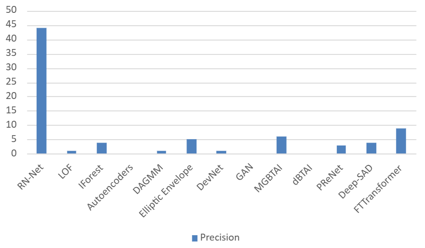
(a) Precision of algorithms on 60 Multivariate Datasets

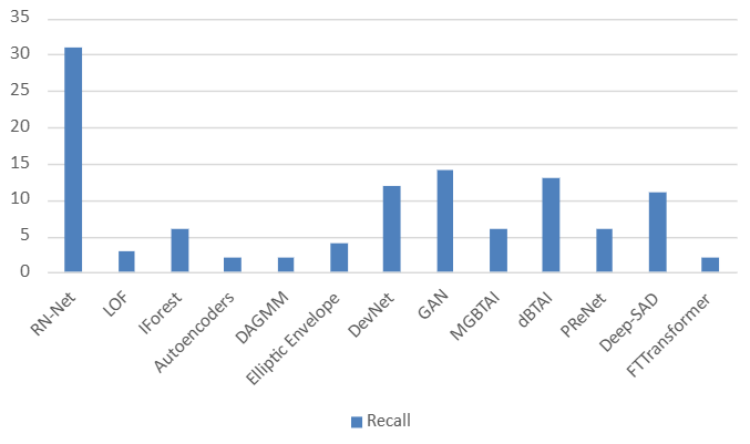
(b) Recall of algorithms on 60 Multivariate Datasets

(c) F1 Scores of algorithms on 60 Multivariate Datasets

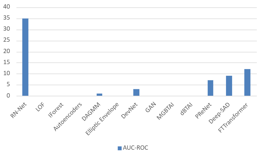
(d) AUC ROC values of algorithms on 60 Multivariate Datasets

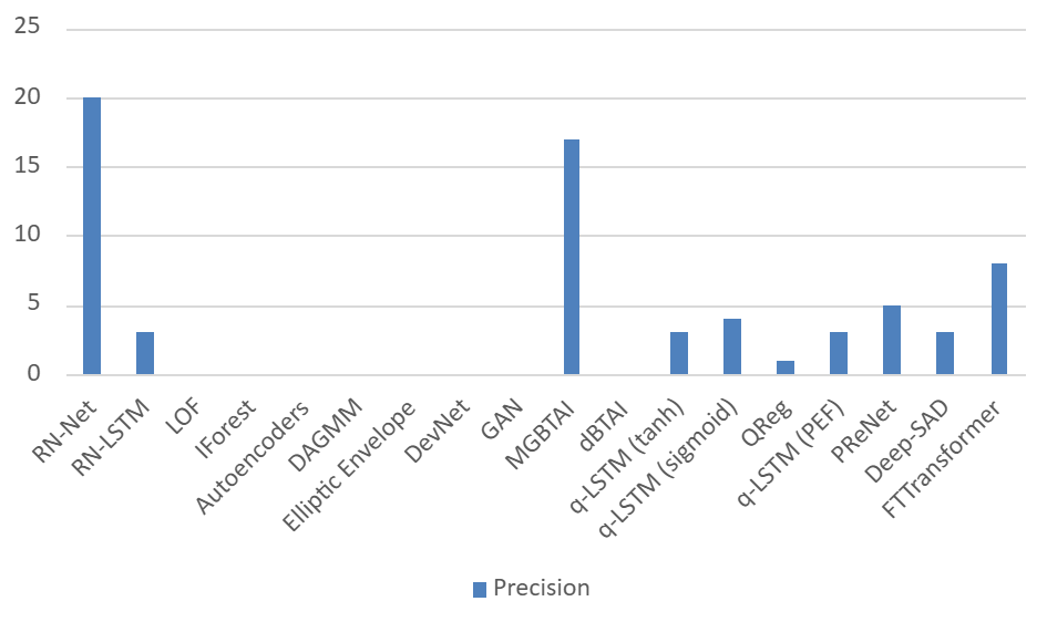
(e) Precision of algorithms on 29 Univariate Time series datasets

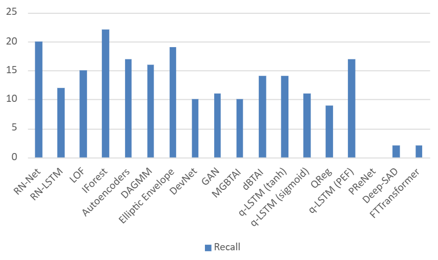
(f) Recall of algorithms on 29 Univariate Time series datasets

(g) F1 Scores of algorithms on 29 Univariate Time series datasets

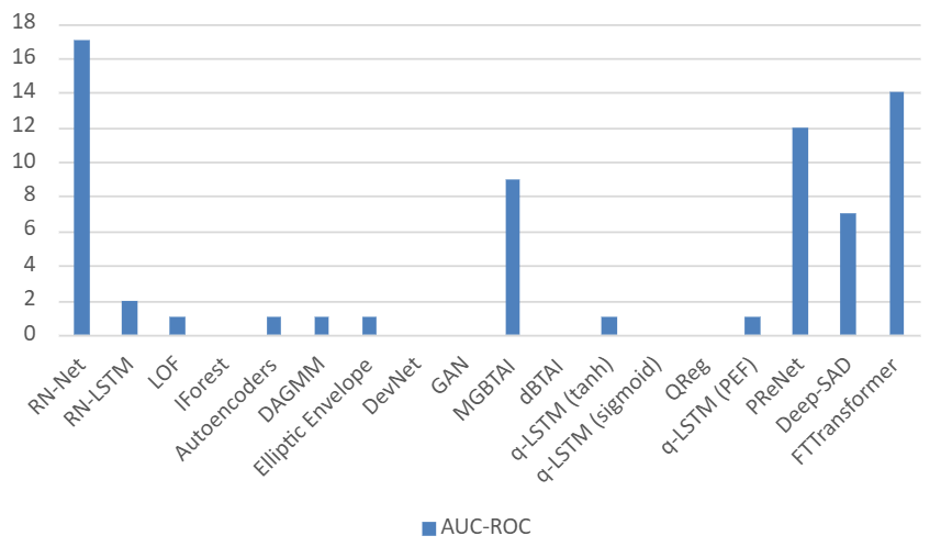
(h) AUC ROC values of algorithms on 29 Univariate Time series datasets

Figure 3: Comparison of algorithm performance on different datasets: (a) Precision, (b) Recall, (c) F1 Scores, and (d) AUC ROC for 60 Multivariate and 29 Univariate Time Series datasets.(Excluding 7 Multivariate Datasets and ESA-ADB dataset)

We trained and tested RN-Net on a total of 60 multivariate datasets(non-timeseries) spanning across various domains. Figures 3(a) through 3(d) present a summary of our results, where we use 9 of the 14 SoTA algorithms; we defer the full results to the Appendix F.

Precision: As deciphered from the figures, RN-Net leads by a significant margin and achieves peak performance in more than 43 datasets out of 60 across all metrics. The proposed algorithm achieves a perfect precision on 8 datasets and hence correctly identifies all outliers.

Recall: As seen in Fig 3(b), Appendix F, the RN-Net model shows exceptional performance by achieving peak recall values in 31 out of 60 datasets, again leaving tree-based approaches and other algorithms lagging behind. The proposed algorithm achieved a perfect recall on 15 datasets, implying no false positives and correctly identifying all outliers.

F-1 Score: As expected from previous results, Fig 3(c), Appendix F, shows that the proposed model attains the maximum F1 score on $44$ datasets because the F1 score is dependent on precision and recall values. The tree-based and other unsupervised algorithms fall short in F1 Scores, demonstrating their under-performance in this metric.

AUC-ROC: We clearly see that RN-Net outperforms every other algorithm by a significant margin (Fig. 3(d), Appendix F. This showcases that it is able to clearly differentiate between the two classes, one of which is less than 10% in some cases. The d-BTAI/MGBTAI algorithms and Elliptic Envelope manages to perform highest in 2 datasets.

The recent state-of-the-art (SoTA) algorithms demonstrate varying performance across multiple datasets. FTTransformer achieves the best results on 8 datasets in terms of precision, 2 datasets for recall, 9 datasets for F1-score, and 7 datasets for AUC-ROC. DeepSAD shows superior performance on 3 datasets for precision, 10 for recall, 9 for F1-score, and 8 for AUC-ROC. Meanwhile, PReNet achieves top performance on 2 datasets in terms of precision, 6 for recall, none for F1-score, and 7 for AUC-ROC. Detailed results can be found in Appendix F.

Time Series - Univariate Datasets

This study considers 29 univariate datasets, varying in size from about 544 to 2500 datapoints with anomaly percentages ranging from 0.04% to 1.47%. These may be single data instances (point anomalies) or a few data points scattered at a reasonable distance from the norm. The varied distributions of these datasets were identified based on chi-square (Appendix F, Table 13).

Precision: As seen from Figure 3(e), Appendix F, RN-Net shows peak precision in 20 datasets. This signifies the capability of correctly identifying many true anomalies out of the total flagged instances, considering the datasets are also critically imbalanced. This is followed by dBTAI/MGBTAI peaking in 17 datasets.

Recall: As seen from the above Figure 3(f), Appendix F, all models show a considerable recall performance in the univariate datasets with a least group minimum of highest in 10 datasets(DevNet). The RN-Net model tops the chart with the best recall in 20 out of 29 datasets, followed by Isolation Forest, qLSTM, dBTAI/MGBTAI, and RN-LSTM, respectively.

F-1 Score: The above-mentioned results give an indication of the results obtained from Figure 3(g), Appendix F, RN-Net outperforms all algorithms in 21/29 datasets based on the F1 score. In the case of tree-based algorithms, the peak is recorded in 7 datasets.

AUC-ROC: RN-Net achieves the highest performance in terms of AUC-ROC values in 17 datasets, closely followed by dBTAI/MGBTAI at 9 datasets, as observed from Figure 3(h), Appendix F.

The recent state-of-the-art (SoTA) algorithms demonstrate varying performance across multiple datasets. FTTransformer achieves the best results on 8 datasets in terms of precision, 2 datasets for recall, none for F1-score, and 14 datasets for AUC-ROC. DeepSAD shows superior performance on 3 datasets for precision, 2 for recall, none for F1-score, and 7 for AUC-ROC. Meanwhile, PReNet achieves top performance on 5 datasets in terms of precision, none for recall, none for F1-score, and 12 for AUC-ROC. Detailed results can be found in Appendix F. Overall, RN-Net has SoTA performance, whereas, though better than most of the algorithms, RN-LSTM struggles a bit, perhaps because of a fixed number of timesteps, extremely low number of anomalies in some datasets, etc., reasons which can be addressed when dealing with the intricacies of an LSTM. However, it satisfies the motive of showcasing RN-loss adaptability and records SoTA performance on some univariate datasets (with less than 1% anomalies).

Time Series - Multivariate Datasets

We propose the RN-LSTM model for Anomaly detection in time series data, which also emphasizes on the flexibility and adaptability of the RN-loss function. The datasets used are SWaT, BATADAL, and ESA-ADB. The Secure Water Treatment (SWaT) plant is a testbed at the Singapore University of Technology and Design Wang et al. [2019][SWaT: A Water Treatment Testbed for Research and Training on ICS Security], and is considered as a world class dataset. Some of the major challenges faced while working with this dataset are covered in the paper, Ahmed et al. [2020]. The results obtained from LOF, IForest, OCSVM, AutoEncoder, DAGMM, Envelope, DevNet, GDNDeng and Hooi [2021](a modified version of GNN specifically created for Multivariate Time series anomaly detection), GAN, MGBTAI, d-BTAI, RN-Net and RN-LSTM in the form of Recall, F1 score and AUC-ROC are recorded in the table Table 39, Appendix F. These algorithms were chosen because of their dominance over others across datasets.

As shown in the table, GAN has perfect recall performance on almost every dataset but has low precision in each of them, as can be seen from the previous table, indicating that it classifies almost every sample as an anomaly, which may lead to increased false alarms. Excluding GAN, Tree-based algorithms like MGBTAI show the highest performance on 4 datasets based on Recall, and GDN shows the best performance on two datasets based on AUC-ROC. OCSVM also performs well, with peak performance in two of the datasets. GDN, specifically designed for the task of anomaly detection in multivariate time series datasets, falls short when compared with RN-LSTM. RN-Net and RN-LSTM perform best on all datasets based on F1 scores and showcase decent performance individually.

The recent state-of-the-art (SoTA) algorithms demonstrate varying performance across multiple datasets. FTTransformer achieves the best results on 1 dataset in terms of precision, none for recall, 3 for F1-score, and 5 datasets for AUC-ROC. DeepSAD shows superior performance on 1 dataset for precision, 1 for recall, 1 for F1-score, and 1 for AUC-ROC. Meanwhile, PReNet achieves top performance on 1 dataset in terms of precision, none for recall, F1-score or AUC-ROC. Detailed results can be found in Appendix F.

5 Conclusion

Anomaly detection is a fundamental problem across multiple domains. Formally, an anomaly is any sample that does not belong to the underlying data distribution. However, identifying anomalies is challenging, particularly when the data distribution exhibits high variability. Despite its importance, the theoretical foundations of anomaly detection remain underexplored.

What is the right principle to design loss function for anomaly detection? We show that the right principle should correct the discrepancies between the distributions. This is easily achieved by weighing the generic loss function with Radon–Nikodým derivative. We prove this by establishing the PAC learnability of anomaly detection. We refer to this approach as RN-Loss. Notably, we show that (supervised) weight-adjusted loss functions and unsupervised Cluster-Based Local Outlier Factor (CBLOF) naturally emerge as performant and conceptual instances of this correction mechanism.

Empirical evaluations across 96 datasets demonstrate that weighting a standard loss function by the Radon–Nikodým derivative enhances performance, making RN-Loss a robust, efficient, and adaptable solution that outperforms state-of-the-art methods under varying anomaly contamination levels.

The integral representation of the weighted loss function via Radon–Nikodým derivative can be used for imbalanced class boundaries. An interesting regularization interpretation can also be handy in future. The sparsity of the derivative implies a sparsity-inducing regularization; conversely, if it is dense, it might be interpreted as a smoothing regularizer.

RN-Loss: A New Measure Theoretic Loss Function for a Generalized, Adaptable Anomaly Detector
(Supplementary Material)

Appendix A Proofs

Statement (Theorem 3.2):

Let $\nu$ denote the measure induced by $D_{XY}^{0.5}$ and $\mu$ denote the measure induced by $D_{XY}^{\alpha}$. Also, let $d\nu=fd\mu$ (absolutely continuous) where $1/b<f<b$ for some $b<\infty$ on the support of $\mu$. Then, there exists a constant $\Delta_{\mu,\nu}$ such that

$$\frac{1}{\Delta_{\mu,\nu}}\leq\frac{R_{D_{XY}^{0.5}}(h)}{R_{D_{XY}^{\alpha}}(h)}\leq\Delta_{\mu,\nu}\quad\text{for all }h,$$ (14)

where $R_{D_{XY}^{\alpha}}(h)=\mathbb{E}_{(\mathbf{x},y)\sim D_{XY}^{\alpha}}\bigl{[}\ell(h(\mathbf{x}),y)\bigr{]}$ and similarly for $R_{D_{XY}^{0.5}}(h)$.

Proof.

Recall, that

$$R_{D_{XY}^{0.5}}(h)=\int\ell(h({\bm{x}},y))d\nu=\int\ell(h({\bm{x}},y))fd\mu\quad and\quad R_{D_{XY}^{\alpha}}=\int\ell(h({\bm{x}},y))d\mu$$ (15)

So, we have

$$\frac{R_{D_{XY}^{0.5}}(h)}{R_{D_{XY}^{\alpha}}(h)}=\frac{\int\ell(h({\bm{x}},y))fd\mu}{\int\ell(h({\bm{x}},y))d\mu}$$ (16)

Now, observe that $\ell$ is taken to be 0-1 loss, $f$ is bounded by $1/b$ and $b$ on the support of $\mu$, and $\int d\mu=1$ (probability measure). Note that the bound $b$ depends on the distributions $\mu,\nu$. Hence, we have

$$\frac{1}{\Delta_{\mu,\nu}}\leq\frac{R_{D_{XY}^{0.5}}(h)}{R_{D_{XY}^{\alpha}}(h)}\leq\Delta_{\mu,\nu}$$ (17)

for some constant $\Delta_{\mu,\nu}$

∎

Appendix B Deriving the Loss function:

Recall,

$D_{X_{B}Y_{B}}$ and $D_{X_{A}Y_{A}}$ be two probability distributions on a measurable space $\mathcal{X}\times\mathcal{Y}$. Denote their respective densities by $p_{B}(x,y)$ and $p_{A}(x,y)$.For any fixed $\alpha\in[0,1]$, we define $D_{XY}^{\alpha}$ by $(1-\alpha)D_{X_{B}Y_{B}}+\alpha D_{X_{A}Y_{A}}$. Denote by $\mu$ the probability measure induced by $D_{XY}^{\alpha}$. Equivalently, $\mu$ has density

$$\mu(x,y)=(1-\alpha)p_{B}(x,y)+\alpha p_{A}(x,y).$$ (18)

We also consider distribution $D_{XY}^{0.5}$, whose induced measure is denoted $\nu$, with density

$$\nu(x,y)=0.5p_{B}(x,y)+0.5p_{A}(x,y)$$ (19)

Assume that $\nu$ is absolutely continuous with respect to $\mu$ $\nu<<\mu$. By the Radon–Nikodým theorem, there is a function $f(x,y)$ such that

$$d\nu=fd\mu\quad\text{or}\quad\frac{d\nu}{d\mu}(x,y)=f(x,y).$$ (20)

Under the usual condition that $\mu(x,y)>0$, we obtain

$$f(x,y)=\frac{\nu(x,y)}{\mu(x,y)}=\frac{0.5p_{B}(x,y)+0.5p_{A}(x,y)}{(1-\alpha)p_{B}(x,y)+\alpha p_{A}(x,y)}.$$ (21)

Using empirical distribution function to estimate $f$:

Let us now assume we have a sample $\{{\bm{x}}^{i},y^{i}\}$ from $D_{XY}^{\alpha}$ where $y^{i}=1$ if it belongs to $D_{X_{B}Y_{B}}$ and $y^{i}=0$ if it belongs to $D_{X_{A}Y_{A}}$. From above we have,

$$f({\bm{x}},+1)=\frac{0.5}{1-\alpha}\quad and\quad f({\bm{x}},0)=\frac{0.5}{\alpha}$$ (22)

If we let the weight of the anomalous class $D_{X_{A}Y_{A}}$ to be $1$, samples from the majority class $D_{X_{B}Y_{B}}$ are reweighted by

$$\omega=\frac{\alpha}{1-\alpha}$$ (23)

Appendix C CBLOF as Radon–Nikodým derivative:

CBLOF (Cluster-Based Local Outlier Factor) is a widely known measure for obtaining anomaly scores which are known to work well empirically. In this section, we provide an explanation of CBLOF using the Radon–Nikodým framework in this article.
Let $\mathcal{X}\subset\mathbb{R}^{d}$ be the data space. Given a sample $S=\{x_{i}\}_{i=1}^{n}$ drawn from a mixture distribution $D_{XY}^{\alpha}$, we aim to assign an anomaly score to each $x\in\mathcal{X}$.

Naive definition of anomaly:

Any point can be considered an anomaly if it lies far-away from the center. A standard assumption which works well in practice is to assume that the base distribution is a mixture of Gaussians. Thus, we have the following anomaly score

$$h^{*}(x)=\operatorname*{arg\,min}_{i}\|x-\mu_{i}\|$$ (24)

where $\mu_{i}$ denotes the centroid of the $i$th Gaussian. In words, if the point is far-away from the closest center, then it would be considered an anomaly.

Using the naive approach for anomaly detection:

The naive definition applied to identify the outliers within this sample is -

• Cluster the sample into clusters $\{C_{1},C_{2},\cdots,C_{m}\}$, obtain the $m$ corresponding means $\mu_{k}$

• Consider only the largest $k<m$ clusters to estimate the density $p_{B}$. This filtering step allows us to estimate $p_{B}$.

• Obtain the scores $h^{*}(x)$ using Equation 24 and the cluster centroids.

Distribution assumption of $h^{*}$:

Let $p_{C_{i}}(x)$ denote the distribution of each cluster $C_{i}$. Implicit in the above formulation is the distribution assumption

$$D_{XY}^{\alpha}=\frac{1}{m}\sum_{i=1}^{m}\frac{1}{|C_{i}|}p_{C_{i}}(x)$$ (25)

The above distribution can be inferred from the assumption made by CBLOF Gao [2009] - the size of the cluster should not matter for anomalies. Remark: As we shall shortly see, this becomes equivalent to having more anomalies in the small cluster.
Furthermore, we assume that each $p_{C_{i}}(x)$ has a distinct support ${S}_{i}$, ensuring that samples do not overlap across clusters,i.e.

$$\mathcal{S}_{i}\cap\mathcal{S}_{j}=\emptyset,\quad\forall i\neq j.$$ (26)

This assumption ensures that each point $x$ belongs uniquely to a single cluster, simplifying density estimation and anomaly detection.

Discrepancy caused by $D_{XY}^{\alpha}$ vs $D_{XY}^{0.5}$:

Following the reasoning from Appendix B, we correct the discrepancy using the Radon–Nikodým derivative. Note that,

$$D_{XY}^{0.5}\equiv\frac{1}{m}\sum_{i=1}^{m}p_{C_{i}}(x)$$ (27)

Then, the Radon–Nikodým derivative can be computed to be

$$f(x)=\sum_{i=1}^{m}|C_{i}|I[x\in C_{i}]$$ (28)

Accordingly, the anomaly score is adjusted to be

$$h^{\dagger}(x)=\begin{cases}|C_{i}|d(x,C_{i}),&\text{if }x\in C_{i},C_{i}\text{ is large}\\ |C_{i}|d(x,C_{L}),&\text{if }x\in C_{i},C_{L}\text{ is the nearest large cluster}\end{cases}$$ (29)

where $C_{L}$ is the closest large cluster. This ensures anomaly scores reflect both distance-based rarity and density ratio correction.

Appendix D ECBLOF as Radon–Nikodým derivative:

ECBLOF (Enhanced Cluster-Based Local Outlier Factor)Sarkar et al. [2021a] is a modified version of CBLOF designed to avoid the bias caused by multiplying the anomaly score with the cluster size. In CBLOF, points in smaller clusters are assigned higher anomaly scores due to this scaling factor, which can lead to biased detection favoring large clusters. In ECBLOF we assume, $D_{XY}^{0.5}=D_{XY}^{\alpha}=\frac{1}{m}\sum_{i=1}^{m}p_{C_{i}}(x)$ implying that both enforce cluster-size invariance, ensuring anomaly scores depend solely on distances, not cluster populations.

Let $\mathcal{X}\subset\mathbb{R}^{d}$ represent the data space. Given a sample $S=\{x_{i}\}_{i=1}^{n}$ drawn from a mixture distribution $D_{XY}^{\alpha}$, the objective is to assign an unbiased anomaly score to each $x\in\mathcal{X}$.

Modifications in ECBLOF compared to CBLOF:

• Elimination of cluster size scaling: In CBLOF, the anomaly score is scaled by the size of the cluster $|C_{i}|$, which biases the score towards larger clusters.

  $$h(x)=|C_{i}|\cdot d(x,C_{i})$$ (30)

  ECBLOF removes this scaling, ensuring that the anomaly score is based purely on the distance from the point to the nearest cluster centroid.

  $$h^{\dagger}(x)=d(x,C_{i})$$ (31)

• Unbiased scoring: By eliminating the cluster size multiplication, ECBLOF avoids favoring larger clusters and provides a more balanced detection of anomalies.

• Handling small clusters: Similar to CBLOF, ECBLOF still identifies small clusters as potential anomaly sources. However, if a point belongs to a small cluster, the distance to the nearest large cluster $C_{L}$ is used to compute its anomaly score:

  $$h^{\dagger}(x)=\begin{cases}d(x,C_{i}),&\text{if }x\in C_{i},C_{i}\text{ is large}\\ d(x,C_{L}),&\text{if }x\in C_{i},C_{L}\text{ is the nearest large cluster}\end{cases}$$ (32)

Distribution assumption in ECBLOF:

Each cluster $C_{i}$ is assumed to be governed by a distinct distribution $p_{C_{i}}(x)$, with disjoint support sets $\mathcal{S}_{i}$ such that:

$$\mathcal{S}_{i}\cap\mathcal{S}_{j}=\emptyset,\quad\forall i\neq j.$$ (33)

The mixture distribution $D_{XY}^{\alpha}$ is given by:

$$D_{XY}^{\alpha}=\frac{1}{m}\sum_{i=1}^{m}p_{C_{i}}(x)$$ (34)

For unbiased anomaly detection, we need the distribution $D_{XY}^{0.5}$:

$$D_{XY}^{0.5}=\frac{1}{m}\sum_{i=1}^{m}p_{C_{i}}(x)$$ (35)

By assuming $D_{XY}^{\alpha}=D_{XY}^{0.5}$, ECBLOF treats all clusters equally in the mixture distribution, removing the bias that favors large clusters in CBLOF; this ensures that anomaly scores depend only on a point’s distance from its cluster centroid, making detection fairer and unbiased.

Thus the Radon–Nikodým derivative reduces to:

$$f(x)=1$$ (36)

Hence, the corrected anomaly score for ECBLOF is given by:

$$h^{\dagger}(x)=d(x,C_{i})$$ (37)

Remark: Unlike in CBLOF, we do not multiply by $|C_{i}|$. This ensures that the score is purely distance-based, without being influenced by cluster size. This ensures a fair and unbiased detection of anomalies.

Appendix E Literature Review

Throughout the years, much research has been conducted in anomaly detection with a multitude of explored methods such as in Sultani et al. [2018], Liu et al. [2023], Shen et al. [2020a], Schmidl et al. [2022a], Farshchi et al. [2018], Maru and Kobayashi [2020], Yoo et al. [2019], Chhabra et al. [2008]. Since then, this interest has increased significantly as various domains such as cybersecurity Ashiku and Dagli [2021], Wenig et al. [2022], fraud detection, and healthcare Roy et al. [2023], Gupta et al. [2014] became more relevant. The work on learning from imbalanced datasets was proposed in AAAI 2000 workshop and highlighted research on two major problems, types of imbalance that hinder the performance of standard classifiers and the suitable approaches for the same. Japkowicz and Stephen [2002] also showed that the class imbalance problem affects not only standard classifiers like decision trees but also Neural Networks and SVMs. The work by Chawla et al. [2003, 2004] gave a further boost to research in imbalanced data classification. Extensive research was done on unsupervised learning methods to address issues such as relying on static thresholds, in turn struggling to adapt to dynamic data, resulting in high false positives and missed anomalies. However, the work by Kiran et al. [2018] observed that unsupervised anomaly detection can be computationally intensive, especially in high-dimensional datasets. Jacob and Tatbul Jacob et al. [2021] delved into explainable anomaly detection in time series using real-world data, yet deep learning-based time-series anomaly detection models were not thoroughly explored well enough. With significant growth in applying various ML algorithms to detect anomalies, there has been an avalanche of anomaly benchmarking data Han et al. [2022], Wenig et al. [2022], Paparrizos et al. [2022], as well as empirical studies of the performances of existing algorithms Huet et al. [2022], Schmidl et al. [2022b] on different benchmark data. Due to the importance of the problem, there have also been efforts to produce benchmarks such as AD-Bench Han et al. [2022] and ESA-ADB Kotowski et al. [2024]. Researchers have critically examined the suitability of evaluation metrics for machine learning methods in anomaly detection. Kim et al. Kim et al. [2022] exposed the limitations of the F1-score with point adjustment, both theoretically and experimentally.

To conclude, recent benchmarking studies, concentrated on deep-learning-based anomaly detection techniques mostly, have not examined the performance across varying types of anomalies, such as singleton/point, small, and significantly large numbers, nor across different data types, including univariate, multivariate, temporal, and non-temporal data. Additionally, there has been a lack of exploration into how anomalies should be identified when their frequency is high. These observations prompt several critical questions. Is the current SoTA algorithm the most effective? Are we reaching the peak in anomaly detection using Deep Learning approaches? Are unsupervised learning algorithms truly better than supervised learning algorithms?

Appendix F Experimental Results and Data

Table 2: Percentage of wins, ties, and losses on F-1 score across all datasets (96). For brevity, other methods that have no wins or ties are not shown. Wins and ties are determined via a Cohen’s d effect size test.

	(RN-Net/LSTM)	LOF	IForest	Ell. Env.	DevNet	GAN	MGBTAI	d-BTAI
wins	76	5	3	0	3	2	2	5
ties	6	0	0	2	0	0	2	0
losses	18	95	97	98	97	98	96	95

Table 3: Percentage of wins, ties, and losses on F-1 score across datasets with different anomaly ratios.For brevity, other methods (such as OCSVM, DevNet and newer methods like PReNet) that have no wins or ties are not shown.

Anomalies $<1\%$ (26)

	(RN-Net/LSTM)	MGBTAI	d-BTAI	FTTransformer
wins	46	14	9	4
ties	45	23	36	0
losses	9	63	55	96

Anomalies $>10\%$ (16)

	(RN-Net/LSTM)	d-BTAI	FTTransformer	DeepSAD
wins	94	6	19	13
ties	6	0	6	0
losses	0	94	75	87

Algorithm	Anomaly Detection Approach
LOF	Uses data point densities to identify an anomaly by measuring how isolated a point is relative to its nearest neighbors in the feature space. Implemented using the Python Outlier Detection (PyOD) library with default parameters. Trained on 70% of data and tested on the entire dataset.
Iforest	Ensemble-based algorithm that isolates anomalies by constructing decision trees. Reported to perform well in high-dimensional data. The algorithm efficiently separates outliers by requiring fewer splits in the decision tree compared to normal data points. Implemented using scikit-learn with default parameters. Trained on 70% of data and tested on the entire dataset.
OCSVM	Constructs a hyperplane in a high-dimensional space to separate normal data from anomalies. Implemented using scikit-learn with default parameters. Trained on 70% normal data, or whatever normal data was available.
AutoEncoder	Anomalies are identified based on the reconstruction errors generated during the encoding-decoding process. Requires training on normal data. Implemented using Keras. Lower threshold set at the 0.75th percentile, and upper threshold at the 99.25th percentile of the Mean Squared Error (MSE) values. Trained on 70% normal data, or whatever normal data was available. Anomalies are detected by comparing the reconstruction error with the predefined thresholds.
DAGMM	Combines .autoencoder and Gaussian mixture models to model the data distribution and identify anomalies. It has a compression network to process low-dimensional representations, and the Gaussian mixture model helps capture data complexity. This algorithm requires at least 2 anomalies to be effective. It is trained on 70% normal data, or whatever normal data was available. Anomalies are detected by calculating anomaly scores, with thresholds set at two standard deviations above and below the mean anomaly score.
LSTM	Trained on a normal time-series data sequence. Acts as a predictor, and the prediction error, drawn from a multivariate Gaussian distribution, detects the likelihood of anomalous behavior. Implemented using Keras. Lower threshold set at the 5th percentile, and upper threshold at the 95th percentile of the Mean Squared Error (MSE) values. Trained on 70% normal data, or whatever normal data was available. Anomalies are detected when the prediction error lies outside the defined thresholds.
qLSTM	Augments LSTM with quantile thresholds to define the range of normal behavior within the data. Implementation follows the methodology described in the authors’ paper, which applies quantile thresholds to LSTM predictions. Anomalies are detected when the prediction error falls outside the defined quantile range.
QREG	A multilayered LSTM-based RNN forecasts quantiles of the target distribution to detect anomalies. The core mathematical principle involves modeling the target variable’s distribution using multiple quantile functions. Lower threshold set at the 0.9th percentile, and upper threshold at the 99.1st percentile of the predicted values. Anomalies are detected when the predicted value lies outside these quantile thresholds. Trained on 70% data and tested on the entire dataset.
Elliptic Envelope	Fits an ellipse around the central multivariate data points, isolating outliers. It needs a contamination parameter of 0.1 by default, with a support fraction of 0.75, and uses Mahalanobis distance for multivariate outlier detection. Implemented using default parameters from the sklearn package. Trained on 70% of data and tested on the entire dataset. Anomalies are detected when data points fall outside the fitted ellipse.
DevNet	A Deep Learning-based model designed specifically for anomaly detection tasks. Implemented using the Deep Learning-based Outlier Detection (DeepOD) library. Anomalies are detected based on the deviation score, with a threshold defined according to the model’s performance and expected anomaly rate. Trained on 70% data and tested on the entire dataset; it requires atleast 2 anomalies in its training set to function, and for optimal performance, it is recommended to include at least 2% anomalies in the training data.
GAN	Creates data distributions and detects anomalies by identifying data points that deviate from the generated distribution. It consists of generator and discriminator networks trained adversarially. Implemented using Keras. All data points whose discriminator score lies in the lowest 10th percentile are considered anomalies. Trained on 70% normal data.
GNN	GDN, which is based on graph neural networks, learns a graph of relationships between parameters and detects deviations from the patterns. Implementation follows the methodology described in the authors’ paper.
MGBTAI	An unsupervised approach that leverages a multi-generational binary tree structure to identify anomalies in data. Minimum clustering threshold set to 20% of the dataset size and leaf level threshold set to 4. Used k-means clustering function. No training data required.
dBTAI	Like MGBTAI, it does not rely on training data. It adapts dynamically as data environments change.The small cluster threshold is set to 2% of the data size. The leaf level threshold is set to 3. The minimum cluster threshold is set to 10% of the data size and the number of clusters are 2 (for KMeans clustering at each split). The split threshold is 0.9 (used in the binary tree function). The anomaly threshold is determined dynamically using the knee/elbow method on the cumulative sum of sorted anomaly scores. The kernel density uses a gaussian kernel with default bandwidth and uses imbalance ratio to weight the density ratios. Used k-means clustering function. No training data required.
FTTransformer	It is a sample adaptation of the original transformer architecture for tabular data. The model transforms all features (categorical and numerical) to embeddings and applies a stack of Transformer layers to the embeddings. However, as stated in the original paper’s Gorishniy et al. [2021] limitations: FTTransformer requires more resources (both hardware and time) for training than simple models such as ResNet and may not be easily scaled to datasets when the number of features is “too large”.
DeepSAD	It is a generalization of the unsupervised Deep SVDD method to the semi-supervised anomaly detection setting and thus needs labeled data for training. It is also considered as an information-theoretic framework for deep anomaly detection.
PReNet	It has a basic ResNet with input and output convolution layers, several residual blocks (ResBlocks) and a recurrent layer implemented using a LSTM. It is particularly created for the task of image deraining as mentioned in Ren et al. [2019].

Table 4: Descriptions and hyperparameter settings of SOTA algorithms benchmarked in this study

Dataset	LOF	IForest	AutoEncoders	DAGMM	Elliptic Envelope	DevNet	GAN	MGBTAI	dBTAI	Deep-Sad	FTT	PReNet	RN-Net
ALOI	0.10	0.04	0.05	0.03	0.03	0.03	0.04	0.04	0.04	0.04	0.04	0.03	0.29
annthyroid	0.26	0.25	0.15	0.24	0.40	0.12	0.09	0.07	0.10	0.46	0.53	0.06	0.73
backdoor	0.11	0.03	0.20	0.21	0.21	0.21	0.21	0.01	NA	NA	NA	NA	0.65
breastw	0.39	0.98	0.27	1.00	1.00	0.86	0.00	0.85	0.89	0.88	0.94	0.97	0.97
campaign	0.07	0.33	0.22	0.30	0.34	0.42	0.21	0.17	0.17	0.23	0.22	0.17	0.76
cardio	0.17	0.48	0.34	0.13	0.40	0.50	0.07	0.48	0.20	0.40	0.39	0.34	0.90
Cardiotocography	0.32	0.48	0.31	0.36	0.48	0.40	0.24	0.80	0.35	0.34	0.66	0.72	0.88
celeba	0.01	0.07	0.02	0.07	0.09	0.19	0.03	0.08	0.03	0.08	0.12	0.13	0.26
cover	0.02	0.05	0.09	0.02	0.01	0.10	0.01	0.00	0.02	0.05	0.03	0.00	1.00
donors	0.21	0.10	0.14	0.50	0.20	0.44	0.04	0.00	NA	1.00	NA	0.59	0.90
fault	0.32	0.49	0.19	0.36	0.24	0.36	0.47	0.42	0.50	0.57	0.45	0.69	0.89
fraud	0.00	0.02	0.02	0.01	0.02	0.02	NA	0.01	0.01	0.05	0.36	0.01	0.19
glass	0.18	0.10	0.09	0.00	0.12	0.00	0.06	0.08	0.11	0.08	0.14	0.05	0.80
Hepatitis	0.25	0.18	0.13	0.25	0.33	0.25	0.20	0.00	0.17	0.57	0.41	0.63	0.71
http	0.00	0.03	0.04	0.04	0.04	0.04	NA	0.05	0.00	0.00	NA	0.04	0.92
InternetAds	0.48	0.64	0.53	0.20	0.63	0.32	0.11	0.98	NA	0.52	NA	0.65	0.84
Ionosphere	0.94	0.96	0.50	0.69	1.00	0.58	0.58	0.44	0.73	0.78	0.63	0.83	0.96
landsat	0.31	0.15	0.19	0.18	0.04	0.24	0.38	0.01	0.25	0.56	0.68	0.78	0.76
letter	0.36	0.08	0.05	0.06	0.17	0.07	0.06	0.11	NA	NA	NA		0.30
Lymphography	0.33	0.40	0.13	0.07	0.38	0.11	0.13	0.43	0.15	0.31	0.56	0.33	0.67
magic.gamma	0.62	0.78	0.55	0.56	0.91	0.78	0.76	0.77	0.60	0.72	0.68	0.62	0.91
mammography	0.08	0.12	0.05	0.15	0.03	0.19	0.01	0.00	NA	0.03	0.06	0.00	0.44
mnist	0.23	0.32	0.19	0.16	0.16	0.47	0.09	0.02	0.17	0.28	0.54	0.35	0.89
musk	0.01	0.25	0.17	0.32	0.31	0.29	0.03	0.23	0.08	0.27	1.00	0.03	0.91
optdigits	0.07	0.05	0.04	0.05	0.00	0.26	0.03	0.33	0.02	0.53	1.00	0.28	1.00
PageBlocks	0.39	0.41	0.29	0.27	0.56	0.17	0.31	0.67	0.17	0.11	0.22	0.17	1.00
pendigits	0.04	0.16	0.13	0.00	0.06	0.23	0.06	0.00	0.04	0.33	0.71	0.22	0.84
Pima	0.32	0.59	0.35	0.45	0.51	0.68	0.15	0.28	0.42	0.51	0.48	0.57	0.40
satellite	0.48	0.93	0.39	0.77	0.96	0.59	0.32	1.00	0.51	0.62	0.91	0.80	0.84
satimage-2	0.03	0.10	0.00	0.08	0.12	0.12	0.01	0.14	0.03	0.77	0.73	0.11	0.95
shuttle	0.00	0.98	0.47	0.51	1.00	0.48	0.07	0.49	0.45	0.80	0.91	0.67	0.64
skin	0.24	0.06	0.08	0.57	0.30	0.76	0.10	0.62	0.33	0.99	0.94	0.89	1.00
smtp	0.00	0.00	0.00	0.00	0.00	0.00	0.00	0.00	0.00	1.00	0.53	0.00	1.00
SpamBase	0.32	0.41	0.41	0.63	0.31	0.76	0.08	0.73	0.66	0.92	0.86	0.81	1.00
speech	0.02	0.02	0.03	0.01	0.02	0.13	0.08	0.01	0.02	0.12	0.02	0.04	0.93
Stamps	0.15	0.23	0.14	0.03	0.11	0.15	0.45	0.13	0.20	0.39	0.81	0.71	0.06
thyroid	0.10	0.19	0.15	0.17	0.23	0.18	0.17	0.13	0.07	0.29	0.36	0.25	0.70
vertebral	0.04	0.03	0.00	0.08	0.00	0.10	0.04	0.00	0.09	0.14	0.21	0.58	0.75
vowels	0.26	0.09	0.11	0.01	0.05	0.19	0.03	0.67	0.08	0.30	0.24	0.31	0.82
Waveform	0.09	0.06	0.11	0.09	0.04	0.07	0.21	0.00	0.04	0.14	0.07	0.08	0.67
WBC	0.09	0.32	0.38	0.35	0.38	0.31	0.06	0.42	0.19	0.30	0.50	0.43	0.36
WDBC	0.27	0.21	0.26	0.24	0.26	0.26	0.01	0.21	0.13	0.83	0.90	0.27	0.56
Wilt	0.10	0.01	0.05	0.10	0.10	0.00	0.05	0.00	0.04	0.08	0.09	0.14	1.00
wine	0.77	0.18	0.50	0.31	0.36	0.45	0.51	0.53	0.25	0.90	0.90	0.69	0.47
WPBC	0.10	0.14	0.25	0.15	0.15	0.18	0.20	0.12	0.26	0.40	0.57	0.55	1.00
yeast	0.27	0.30	0.35	0.36	0.26	0.35	0.49	0.10	0.30	0.36	0.46	0.34	0.82
CIFAR10	0.14	0.13	0.07	0.05	0.13	0.17	0.18	0.04	0.08	0.10	0.08	0.06	0.81
FashionMNIST	0.15	0.19	0.12	0.11	0.18	0.29	0.21	0.06	0.10	0.22	0.15	0.12	0.33
MNIST-C	0.13	0.08	0.04	0.08	0.08	0.38	0.09	0.05	0.10	0.49	0.31	0.27	0.97
MVTec-AD	0.87	1.00	0.50	0.40	0.12	0.26	0.97	1.00	0.77	0.93	1.00	1.00	0.96
SVHN	0.11	0.06	0.04	0.05	0.09	0.38	0.10	0.06	0.07	0.14	0.07	0.09	0.49
Agnews	0.11	0.06	0.05	0.06	0.07	0.07	0.10	0.05	0.06	0.09	0.05	0.16	0.33
Amazon	0.06	0.06	0.05	0.05	0.06	0.06	0.06	0.05	0.06	0.01	0.06	0.18	0.23
Imdb	0.04	0.04	0.05	0.05	0.03	0.07	0.00	0.02	0.05	0.09	0.00	0.09	0.36
Yelp	0.10	0.09	0.03	0.06	0.07	0.06	0.04	0.04	0.07	0.13	0.11	0.08	0.36
20newsgroups	0.18	0.07	0.05	0.06	0.10	0.05	0.04	0.00	0.08	0.08	0.05	0.14	0.41
BATADAL 04	0.20	0.10	0.09	0.19	0.26	0.05	0.10	0.10	0.10	0.13	0.07	0.17	0.17
SWaT 1	0.08	0.63	0.13	0.50	0.19	0.22	0.09	0.63	0.19	0.51	0.17	0.21	0.40
SWaT 2	0.06	0.71	0.10	0.11	0.13	0.12	0.05	0.71	0.06	0.07	0.25	0.08	0.33
SWaT 3	0.04	0.02	0.13	0.23	0.09	0.15	0.04	0.02	NA	NA	NA	NA	0.66
SWaT 4	0.45	0.34	0.08	0.99	0.27	0.88	0.44	0.34	0.19	1.00	1.00	1.00	0.85
SWaT 5	0.02	0.22	0.09	0.10	0.12	0.12	0.03	0.22	0.06	0.15	0.17	0.03	0.36
SWaT 6	0.07	0.97	0.37	0.26	0.26	0.17	0.06	0.97	0.13	0.32	0.92	0.33	0.21
ecoli	0.21	0.19	0.20	0.22	0.21	0.06	0.00	0.14	0.04	0.12	0.21	0.21	0.44
cmc	0.01	0.00	0.03	0.01	0.01	0.00	0.05	0.00	0.01	0.03	0.02	0.03	0.15
lympho h	0.33	0.32	0.12	0.00	0.21	0.06	0.05	0.00	0.10	0.43	0.33	0.40	0.64
wbc h	0.37	0.34	0.27	0.32	0.35	0.40	0.04	0.61	0.15	0.06	0.38	0.37	0.85

Table 5: Precision value comparison on Multivariate datasets

Dataset	LOF	Iforest	AutoEncoders	DAGMM	Elliptic Envelope	DevNet	GAN	MGBTAI	dBTAI	Deep-Sad	FTT	PReNet	RN-Net
ALOI	0.34	0.15	0.12	0.11	0.09	0.08	0.14	0.13	0.41	0.16	0.18	0.11	0.57
annthyroid	0.35	0.41	0.20	0.32	0.52	0.17	0.12	0.18	0.49	0.62	0.09	0.08	0.83
backdoor	0.45	0.16	0.19	0.87	0.84	0.91	0.86	0.02	NA	NA	NA	NA	0.98
breastw	1.00	0.41	0.13	0.29	0.32	1.00	0.00	0.33	0.85	0.95	0.98	0.28	0.95
campaign	0.06	0.35	0.19	0.27	0.31	0.52	0.19	0.16	0.64	0.57	0.19	0.15	0.51
cardio	0.18	0.61	0.36	0.14	0.42	0.79	0.07	0.32	0.76	0.78	0.41	0.36	0.89
Cardiotocography	0.15	0.26	0.13	0.16	0.21	0.23	0.32	0.20	0.47	0.05	0.29	0.33	0.70
celeba	0.05	0.38	0.10	0.29	0.38	0.88	0.15	0.70	0.37	0.74	0.52	0.58	0.90
cover	0.22	0.57	0.37	0.24	0.13	0.97	1.00	0.00	0.69	0.25	0.91	0.04	1.00
donors	0.33	0.20	0.24	0.86	0.33	1.00	0.10	0.00	NA	0.99	NA	1.00	1.00
fault	0.09	0.18	0.24	0.10	0.07	0.11	0.14	0.07	0.63	0.62	0.59	0.20	0.44
fraud	0.11	0.89	0.88	0.62	0.85	0.92	NA	0.62	0.85	0.84	0.80	0.83	0.83
glass	0.44	0.33	0.22	0.00	0.33	0.00	0.13	0.11	0.78	0.67	0.67	0.11	1.00
Hepatitis	0.15	0.15	0.08	0.15	0.31	0.15	0.12	0.00	0.31	1.00	0.69	0.38	0.83
http	0.03	1.00	1.00	1.00	1.00	1.00	NA	1.00	0.02	1.00	NA	1.00	0.95
InternetAds	0.26	0.42	0.29	0.11	0.36	0.17	0.04	0.23	NA	0.85	NA	0.35	0.86
Ionosphere	0.26	0.35	0.14	0.20	0.25	0.25	0.16	0.03	0.78	0.91	0.84	0.24	0.89
landsat	0.15	0.09	0.09	0.09	0.02	0.12	0.19	0.00	0.44	0.78	0.46	0.38	0.80
letter	0.57	0.16	0.08	0.09	0.28	0.12	0.10	0.18	NA	NA	NA	NA	0.80
Lymphography	0.83	1.00	0.33	0.17	0.83	0.33	0.33	1.00	1.00	0.83	0.83	0.83	0.67
magic.gamma	0.18	0.26	0.16	0.16	0.26	0.57	0.22	0.21	0.49	0.79	0.73	0.18	0.45
mammography	0.37	0.64	0.42	0.64	0.13	0.80	0.04	0.00	NA	0.55	0.25	0.01	0.71
mnist	0.25	0.42	0.21	0.18	0.18	0.71	1.00	0.02	0.85	0.85	0.88	0.38	0.94
musk	0.04	1.00	0.53	1.00	1.00	1.00	1.00	0.79	1.00	0.97	0.99	1.00	0.90
optdigits	0.26	0.21	0.15	0.16	0.01	0.99	0.12	0.81	0.34	0.97	0.98	0.99	1.00
PageBlocks	0.41	0.52	0.30	0.29	0.61	0.20	0.33	0.06	0.21	0.89	0.80	0.18	1.00
pendigits	0.17	0.88	0.56	0.01	0.28	0.98	0.25	0.03	0.71	0.99	0.97	0.97	0.64
Pima	0.09	0.23	0.10	0.13	0.16	0.36	0.04	0.05	0.44	0.73	0.63	0.16	0.98
satellite	0.15	0.34	0.12	0.24	0.29	0.31	1.00	0.30	0.59	0.56	0.64	0.25	0.48
satimage-2	0.28	0.99	0.01	0.65	1.00	0.97	1.00	1.00	1.00	0.93	0.92	0.93	0.90
shuttle	0.00	0.41	0.65	0.72	0.31	0.98	1.00	0.01	0.89	0.48	0.97	0.94	1.00
skin	0.12	0.03	0.04	0.28	0.14	1.00	0.05	0.15	0.33	0.99	0.45	0.43	1.00
smtp	0.70	0.77	0.70	0.87	0.77	0.70	1.00	0.33	0.87	0.57	0.63	0.67	0.62
SpamBase	0.08	0.12	0.10	0.16	0.07	0.45	0.02	0.18	0.27	0.06	0.21	0.20	0.72
speech	0.15	0.15	0.18	0.03	0.11	0.75	0.12	0.11	0.51	0.97	0.57	0.25	0.78
Stamps	0.16	0.32	0.15	0.03	0.13	0.16	0.49	0.06	0.84	0.77	0.81	0.77	0.71
thyroid	0.39	0.97	0.62	0.71	0.96	0.72	0.71	0.25	0.92	0.91	0.99	1.00	0.96
vertebral	0.03	0.03	0.00	0.07	0.00	0.07	0.03	0.00	0.24	0.93	0.53	0.47	1.00
vowels	0.76	0.30	0.33	0.02	0.14	0.62	0.08	0.16	1.00	0.78	0.74	0.90	0.69
Waveform	0.31	0.25	0.37	0.32	0.16	0.24	0.72	0.00	0.71	0.51	0.13	0.27	1.00
WBC	0.20	1.00	0.90	0.80	1.00	1.00	0.13	1.00	1.00	0.90	0.90	1.00	0.58
WDBC	1.00	1.00	1.00	0.90	0.90	1.00	0.33	1.00	1.00	1.00	0.90	1.00	1.00
Wilt	0.19	0.02	0.10	0.18	0.20	0.00	1.00	0.00	0.17	0.51	0.86	0.26	1.00
wine	1.00	0.30	0.70	0.40	0.40	1.00	0.67	1.00	1.00	0.90	0.90	0.90	0.78
WPBC	0.04	0.09	0.11	0.06	0.06	0.06	0.09	0.04	0.45	0.72	0.26	0.23	1.00
yeast	0.08	0.10	0.10	0.11	0.08	0.10	0.14	0.00	0.30	0.82	0.50	0.10	0.80
CIFAR10	0.27	0.31	0.14	0.10	0.26	0.37	0.37	0.07	0.70	0.61	0.36	0.13	0.74
FashionMNIST	0.30	0.47	0.24	0.22	0.36	0.71	0.42	0.12	0.93	0.80	0.59	0.24	0.63
MNIST-C	0.27	0.18	0.08	0.15	0.15	0.97	0.18	0.12	0.88	0.88	0.83	0.54	0.99
MVTec-AD	0.41	0.51	0.24	0.19	0.21	0.13	0.46	0.22	0.90	0.62	0.48	0.48	0.91
SVHN	0.22	0.13	0.08	0.10	0.20	0.96	0.20	0.06	0.62	0.50	0.46	0.18	0.59
Agnews	0.22	0.15	0.09	0.12	0.14	0.14	0.21	0.02	0.47	0.59	1.00	0.33	0.73
Amazon	0.12	0.14	0.10	0.11	0.12	0.12	0.11	0.12	0.46	0.21	0.35	0.36	0.54
Imdb	0.08	0.08	0.10	0.10	0.06	0.13	0.00	0.02	0.33	0.19	0.00	0.19	0.64
Yelp	0.20	0.21	0.07	0.11	0.14	0.11	0.08	0.04	0.57	0.25	0.09	0.17	0.51
20newsgroups	0.37	0.17	0.11	0.13	0.19	0.10	0.08	0.00	0.60	0.71	0.95	0.27	0.54
BATADAL 04	0.38	0.10	0.17	0.36	0.50	0.10	0.23	0.10	0.75	0.76	0.42	0.32	0.37
SWaT 1	0.09	0.15	0.15	0.57	0.21	0.23	1.00	0.15	0.79	0.59	0.91	0.24	0.40
SWaT 2	0.13	0.08	0.20	0.23	0.27	0.26	1.00	0.08	0.43	0.75	0.92	0.17	0.31
SWaT 3	0.12	0.03	0.38	0.65	0.24	0.42	1.00	0.03	NA	NA	NA	NA	0.79
SWaT 4	0.10	0.12	0.02	0.23	0.06	0.89	1.00	0.12	0.15	0.90	0.98	0.23	0.04
SWaT 5	0.08	0.22	0.36	0.38	0.51	0.50	1.00	0.22	0.85	0.40	0.94	0.11	0.55
SWaT 6	0.12	0.40	0.63	0.44	0.44	0.30	1.00	0.40	0.80	0.79	1.00	0.56	0.72
ecoli	0.78	0.78	0.78	0.78	0.78	0.22	0.00	0.78	0.56	0.67	0.78	0.78	1.00
cmc	0.06	0.00	0.24	0.06	0.12	0.00	0.47	0.00	0.18	0.94	0.65	0.29	1.00
lympho h	0.83	1.00	0.33	0.00	0.67	0.17	0.11	0.00	1.00	1.00	0.67	1.00	0.80
wbc h	0.67	0.71	0.48	0.57	0.67	1.00	0.08	0.52	0.95	1.00	0.86	0.67	1.00

Table 6: Recall value comparison on Multivariate datasets

Dataset	LOF	Iforest	AutoEncoders	DAGMM	Elliptic Envelope	DevNet	GAN	MGBTAI	dBTAI	Deep-Sad	FTT	PReNet	RN-Net
ALOI	0.16	0.06	0.06	0.05	0.04	0.04	0.06	0.07	0.07	0.07	0.06	0.05	0.39
annthyroid	0.30	0.31	0.17	0.28	0.45	0.14	0.10	0.10	0.17	0.39	0.53	0.07	0.78
backdoor	0.18	0.05	0.26	0.34	0.33	0.35	0.34	0.02	NA	NA	NA	NA	0.78
breastw	0.56	0.57	0.26	0.45	0.49	0.92	0.00	0.48	0.87	0.92	0.96	0.44	0.96
campaign	0.06	0.34	0.20	0.28	0.32	0.47	0.20	0.16	0.27	0.33	0.20	0.16	0.61
cardio	0.18	0.54	0.35	0.13	0.41	0.61	0.07	0.38	0.32	0.53	0.40	0.35	0.90
Cardiotocography	0.20	0.34	0.19	0.22	0.29	0.29	0.22	0.32	0.40	0.09	0.41	0.45	0.78
celeba	0.02	0.12	0.04	0.11	0.14	0.32	0.05	0.14	0.06	0.15	0.19	0.21	0.41
cover	0.04	0.09	0.17	0.04	0.02	0.17	0.02	0.00	0.04	0.08	0.06	0.01	1.00
donors	0.26	0.13	0.19	0.63	0.25	0.61	0.06	0.00	NA	0.99	NA	0.74	0.95
fault	0.15	0.26	0.38	0.16	0.11	0.16	0.21	0.12	0.56	0.59	0.52	0.31	0.59
fraud	0.00	0.03	0.03	0.02	0.04	0.03	NA	0.02	0.01	0.09	0.49	0.03	0.31
glass	0.26	0.16	0.13	0.00	0.18	0.00	0.08	0.09	0.20	0.15	0.23	0.06	0.89
Hepatitis	0.19	0.17	0.10	0.19	0.32	0.19	0.15	0.00	0.22	0.72	0.51	0.48	0.77
http	0.00	0.06	0.07	0.07	0.07	0.08	NA	0.08	0.00	0.01	NA	0.07	0.94
InternetAds	0.33	0.42	0.37	0.14	0.46	0.22	0.16	0.38	NA	0.65	NA	0.45	0.85
Ionosphere	0.41	0.51	0.22	0.31	0.39	0.35	0.25	0.06	0.75	0.84	0.72	0.37	0.92
landsat	0.20	0.11	0.13	0.12	0.02	0.16	0.25	0.00	0.32	0.65	0.55	0.51	0.78
letter	0.57	0.11	0.06	0.07	0.22	0.09	0.07	0.13	NA	NA	NA	NA	0.32
Lymphography	0.48	0.57	0.18	0.10	0.53	0.17	0.19	0.60	0.26	0.45	0.67	0.48	0.67
magic.gamma	0.27	0.39	0.24	0.25	0.40	0.66	0.34	0.33	0.54	0.75	0.70	0.27	0.60
mammography	0.14	0.21	0.09	0.24	0.05	0.30	0.02	0.00	NA	0.12	0.09	0.00	0.54
mnist	0.24	0.37	0.20	0.17	0.17	0.56	0.17	0.02	0.28	0.42	0.67	0.36	0.91
musk	0.02	0.39	0.25	0.48	0.47	0.45	0.06	0.35	0.15	0.42	0.99	0.06	0.91
optdigits	0.12	0.08	0.07	0.07	0.00	0.42	0.05	0.47	0.04	0.68	0.99	0.44	1.00
PageBlocks	0.40	0.46	0.30	0.28	0.58	0.18	0.32	0.11	0.19	0.20	0.34	0.17	1.00
pendigits	0.06	0.28	0.21	0.00	0.11	0.37	0.09	0.00	0.07	0.49	0.82	0.36	0.73
Pima	0.14	0.33	0.16	0.20	0.24	0.47	0.07	0.09	0.43	0.60	0.54	0.26	0.57
satellite	0.23	0.50	0.19	0.37	0.45	0.41	0.48	0.46	0.55	0.59	0.75	0.39	0.61
satimage-2	0.28	0.18	0.00	0.14	0.21	0.22	0.02	0.25	0.07	0.84	0.81	0.20	0.92
shuttle	0.00	0.57	0.54	0.60	0.48	0.64	0.13	0.01	0.59	0.59	0.94	0.79	0.78
skin	0.16	0.04	0.05	0.37	0.19	0.86	0.07	0.24	0.33	0.99	0.61	0.58	1.00
smtp	0.00	0.00	0.00	0.01	0.01	0.00	0.00	0.00	0.00	0.72	0.58	0.00	0.76
SpamBase	0.13	0.18	0.16	0.25	0.12	0.57	0.03	0.29	0.38	0.11	0.34	0.32	0.84
speech	0.04	0.04	0.05	0.01	0.03	0.23	0.03	0.03	0.03	0.21	0.04	0.07	0.85
Stamps	0.15	0.27	0.14	0.03	0.12	0.15	0.47	0.09	0.32	0.52	0.81	0.74	0.10
thyroid	0.15	0.32	0.24	0.28	0.37	0.29	0.28	0.17	0.12	0.43	0.53	0.39	0.81
vertebral	0.04	0.03	0.00	0.07	0.00	0.08	0.04	0.00	0.13	0.24	0.30	0.52	0.86
vowels	0.39	0.14	0.17	0.01	0.07	0.30	0.04	0.26	0.14	0.43	0.37	0.46	0.75
Waveform	0.14	0.09	0.17	0.14	0.07	0.11	0.32	0.00	0.08	0.22	0.09	0.12	0.80
WBC	0.12	0.49	0.53	0.48	0.56	0.48	0.08	0.57	0.31	0.45	0.64	0.61	0.45
WDBC	0.43	0.35	0.42	0.38	0.40	0.41	0.02	0.34	0.23	0.91	0.90	0.43	0.72
Wilt	0.14	0.01	0.07	0.12	0.13	0.00	0.10	0.00	0.07	0.14	0.17	0.18	1.00
wine	0.87	0.22	0.58	0.35	0.38	0.55	0.58	0.69	0.40	0.90	0.90	0.78	0.59
WPBC	0.06	0.11	0.15	0.09	0.09	0.09	0.12	0.06	0.33	0.52	0.35	0.33	1.00
yeast	0.12	0.16	0.16	0.16	0.12	0.16	0.22	0.01	0.30	0.50	0.48	0.16	0.81
CIFAR10	0.18	0.18	0.09	0.07	0.18	0.23	0.25	0.05	0.14	0.18	0.13	0.09	0.77
FashionMNIST	0.20	0.27	0.16	0.15	0.24	0.41	0.28	0.08	0.19	0.34	0.24	0.16	0.43
MNIST-C	0.18	0.11	0.06	0.10	0.10	0.55	0.12	0.07	0.18	0.63	0.45	0.36	0.98
MVTec-AD	0.56	0.67	0.32	0.26	0.15	0.17	0.62	0.36	0.83	0.74	0.65	0.65	0.93
SVHN	0.15	0.08	0.06	0.06	0.13	0.55	0.12	0.06	0.13	0.22	0.12	0.12	0.53
Agnews	0.15	0.09	0.06	0.08	0.09	0.09	0.14	0.03	0.11	0.16	0.10	0.22	0.46
Amazon	0.08	0.08	0.07	0.07	0.08	0.08	0.07	0.07	0.11	0.14	0.10	0.24	0.32
Imdb	0.06	0.05	0.07	0.07	0.04	0.09	0.00	0.02	0.08	0.12	0.00	0.12	0.46
Yelp	0.13	0.12	0.06	0.07	0.10	0.07	0.06	0.04	0.13	0.17	0.10	0.11	0.42
20newsgroups	0.25	0.10	0.09	0.09	0.13	0.06	0.06	0.00	0.14	0.15	0.09	0.18	0.46
BATADAL 04	0.26	0.10	0.12	0.25	0.34	0.07	0.14	0.10	0.18	0.22	0.12	0.22	0.23
SWaT 1	0.09	0.24	0.14	0.53	0.20	0.22	0.16	0.24	0.30	0.55	0.29	0.22	0.40
SWaT 2	0.08	0.15	0.13	0.15	0.18	0.16	0.04	0.15	0.11	0.13	0.40	0.11	0.30
SWaT 3	0.06	0.02	0.20	0.34	0.13	0.23	0.04	0.02	NA	NA	NA	NA	0.69
SWaT 4	0.17	0.18	0.03	0.37	0.10	0.89	0.44	0.18	0.17	0.94	0.99	0.37	0.08
SWaT 5	0.03	0.22	0.15	0.15	0.20	0.17	0.02	0.22	0.12	0.22	0.29	0.04	0.43
SWaT 6	0.09	0.57	0.46	0.33	0.32	0.20	0.06	0.57	0.22	0.46	0.96	0.41	0.32
ecoli	0.33	0.30	0.31	0.33	0.21	0.10	0.00	0.23	0.07	0.19	0.33	0.33	0.60
cmc	0.01	0.00	0.06	0.01	0.03	0.00	0.10	0.00	0.01	0.06	0.04	0.06	0.27
lympho h	0.48	0.48	0.18	0.00	0.32	0.09	0.07	0.00	0.19	0.60	0.44	0.57	0.64
wbc h	0.47	0.46	0.35	0.41	0.46	0.57	0.06	0.56	0.25	0.11	0.52	0.47	0.92

Table 7: F1 Scores comparison on Multivariate datasets

Dataset	LOF	Iforest	AutoEncoders	DAGMM	Elliptic Envelope	DevNet	GAN	MGBTAI	dBTAI	Deep-Sad	FTT	PReNet	RN-Net
ALOI	0.63	0.51	0.51	0.51	0.49	0.49	0.52	0.52	0.53	0.57	0.50	0.51	0.71
annthyroid	0.63	0.66	0.55	0.62	0.73	0.54	0.51	0.50	0.57	0.90	0.51	0.47	0.93
backdoor	0.68	0.52	0.53	0.89	0.88	0.91	0.89	0.49	NA	NA	NA	NA	0.99
breastw	0.57	0.70	0.63	0.64	0.66	0.95	0.41	0.65	0.90	0.97	0.99	0.83	0.98
campaign	0.48	0.63	0.55	0.59	0.62	0.72	0.55	0.53	0.62	0.71	0.68	0.65	0.71
cardio	0.55	0.77	0.64	0.52	0.68	0.85	0.40	0.64	0.72	0.89	0.81	0.82	0.96
Cardiotocography	0.53	0.59	0.55	0.54	0.57	0.67	0.50	0.59	0.61	0.38	0.69	0.77	0.84
celeba	0.47	0.63	0.50	0.60	0.64	0.90	0.52	0.75	0.55	0.87	0.76	0.81	0.89
cover	0.56	0.73	0.91	0.57	0.52	0.94	0.50	0.50	0.68	0.39	0.89	0.66	1.00
donors	0.63	0.54	0.60	0.90	0.62	0.96	0.47	0.50	NA	1.00	NA	0.99	0.98
fault	0.50	0.54	0.68	0.50	0.48	0.50	0.53	0.51	0.65	0.75	0.63	0.53	0.68
fraud	0.51	0.88	0.89	0.77	0.88	0.91	NA	0.75	0.72	0.93	0.92	0.93	0.92
glass	0.68	0.60	0.56	0.50	0.61	0.50	0.52	0.53	0.75	0.73	0.82	0.83	0.99
Hepatitis	0.53	0.51	0.49	0.53	0.59	0.53	0.51	0.44	0.51	0.97	0.77	0.65	0.83
http	0.47	0.94	0.95	0.95	0.95	0.95	NA	0.95	0.34	0.01	NA	1.00	0.95
InternetAds	0.60	0.68	0.61	0.50	0.66	0.54	0.47	0.62	NA	0.91	NA	0.51	0.93
Ionosphere	0.63	0.67	0.53	0.57	0.62	0.57	0.55	0.50	0.81	0.94	0.84	0.41	0.97
landsat	0.53	0.48	0.50	0.49	0.45	0.51	0.55	0.44	0.55	0.88	0.76	0.61	0.88
letter	0.75	0.52	0.49	0.49	0.60	0.51	0.50	0.54	NA	NA	NA	NA	0.84
Lymphography	0.88	0.97	0.62	0.53	0.89	0.61	0.62	0.97	0.88	0.92	1.00	0.83	0.74
magic.gamma	0.56	0.61	0.54	0.55	0.62	0.74	0.59	0.59	0.66	0.88	0.85	0.59	0.63
mammography	0.64	0.77	0.58	0.78	0.52	0.86	0.47	0.50	NA	0.67	0.77	0.31	0.89
mnist	0.58	0.67	0.56	0.54	0.54	0.82	0.50	0.46	0.71	0.89	0.96	0.43	0.98
musk	0.47	0.95	0.72	0.96	0.96	0.96	0.50	0.85	0.81	0.98	1.00	0.50	0.97
optdigits	0.58	0.55	0.52	0.53	0.45	0.96	0.51	0.88	0.44	0.99	1.00	0.99	1.00
PageBlocks	0.67	0.72	0.61	0.60	0.78	0.55	0.62	0.53	0.55	0.49	0.82	0.40	1.00
pendigits	0.53	0.89	0.74	0.46	0.59	0.95	0.58	0.41	0.65	0.99	0.99	0.99	0.79
Pima	0.49	0.57	0.50	0.52	0.54	0.64	0.46	0.49	0.56	0.73	0.65	0.52	0.99
satellite	0.54	0.66	0.52	0.60	0.64	0.61	0.50	0.65	0.67	0.73	0.80	0.61	0.70
satimage-2	0.59	0.94	0.46	0.78	0.95	0.94	0.50	0.92	0.83	0.99	0.99	0.97	0.97
shuttle	0.43	0.70	0.80	0.83	0.66	0.95	0.50	0.50	0.90	0.76	0.99	0.97	1.00
skin	0.51	0.45	0.46	0.61	0.53	0.96	0.47	0.56	0.58	0.99	0.84	0.97	1.00
smtp	0.80	0.82	0.80	0.88	0.83	0.80	0.50	0.64	0.79	0.81	0.77	0.79	0.76
SpamBase	0.48	0.50	0.50	0.55	0.48	0.68	0.43	0.57	0.59	0.41	0.74	0.69	0.84
speech	0.52	0.51	0.54	0.47	0.51	0.84	0.51	0.49	0.48	0.98	0.52	0.51	0.91
Stamps	0.53	0.61	0.53	0.46	0.51	0.53	0.72	0.51	0.75	0.90	0.93	0.94	0.57
thyroid	0.65	0.93	0.76	0.81	0.94	0.82	0.81	0.60	0.80	0.98	1.00	1.00	0.94
vertebral	0.46	0.44	0.44	0.48	0.44	0.49	0.31	0.49	0.44	0.42	0.65	0.75	1.00
vowels	0.84	0.60	0.62	0.46	0.52	0.76	0.49	0.58	0.79	0.94	0.91	0.96	0.89
Waveform	0.61	0.56	0.64	0.61	0.53	0.57	0.82	0.50	0.61	0.77	0.51	0.65	0.99
WBC	0.55	0.95	0.91	0.86	0.96	0.95	0.52	0.97	0.90	0.98	0.99	0.98	0.82
WDBC	0.96	0.95	0.96	0.91	0.91	0.96	0.46	0.95	0.91	1.00	1.00	1.00	0.97
Wilt	0.55	0.44	0.50	0.54	0.55	0.45	0.50	0.48	0.48	0.58	0.73	0.65	1.00
wine	0.99	0.59	0.82	0.66	0.67	0.95	0.81	0.96	0.87	0.98	1.00	1.00	0.88
WPBC	0.46	0.46	0.50	0.48	0.48	0.49	0.49	0.47	0.52	0.75	0.58	0.66	1.00
yeast	0.48	0.49	0.50	0.50	0.48	0.50	0.53	0.49	0.47	0.53	0.61	0.49	0.87
CIFAR10	0.59	0.60	0.52	0.50	0.59	0.68	0.64	0.49	0.64	0.72	0.58	0.52	0.77
FashionMNIST	0.60	0.68	0.58	0.56	0.64	0.81	0.67	0.51	0.76	0.90	0.73	0.60	0.72
MNIST-C	0.59	0.53	0.49	0.53	0.53	0.94	0.54	0.50	0.73	0.97	0.93	0.76	1.00
MVTec-AD	0.70	0.75	0.59	0.56	0.39	0.51	0.73	0.61	0.92	0.86	0.90	0.95	0.97
SVHN	0.56	0.51	0.49	0.50	0.55	0.94	0.58	0.51	0.59	0.72	0.59	0.58	0.81
Agnews	0.56	0.51	0.50	0.51	0.52	0.51	0.56	0.50	0.55	0.68	0.42	0.73	0.81
Amazon	0.51	0.51	0.50	0.50	0.51	0.51	0.51	0.50	0.55	0.63	0.51	0.75	0.67
Imdb	0.49	0.48	0.50	0.50	0.48	0.52	0.50	0.48	0.48	0.59	0.45	0.58	0.79
Yelp	0.55	0.55	0.48	0.51	0.52	0.51	0.49	0.50	0.59	0.66	0.44	0.58	0.68
20newsgroups	0.64	0.53	0.51	0.52	0.55	0.50	0.49	0.50	0.62	0.69	0.43	0.71	0.75
BATADAL 04	0.65	0.52	0.54	0.64	0.71	0.50	0.55	0.52	0.69	0.80	0.56	0.64	0.57
SWaT 1	0.50	0.57	0.53	0.76	0.56	0.57	0.50	0.57	0.73	0.76	0.78	0.49	0.54
SWaT 2	0.51	0.54	0.55	0.57	0.59	0.58	0.50	0.54	0.55	0.64	0.96	0.44	0.56
SWaT 3	0.51	0.48	0.64	0.79	0.57	0.66	0.50	0.48	NA	NA	NA	NA	0.81
SWaT 4	0.50	0.47	0.43	0.61	0.47	0.90	0.50	0.47	0.32	0.96	1.00	0.95	0.07
SWaT 5	0.49	0.60	0.63	0.65	0.71	0.70	0.50	0.60	0.76	0.60	0.96	0.49	0.64
SWaT 6	0.51	0.70	0.78	0.68	0.68	0.60	0.50	0.70	0.73	0.89	1.00	0.84	0.82
ecoli	0.85	0.84	0.83	0.85	0.85	0.57	0.50	0.82	0.59	0.86	0.90	0.92	0.99
cmc	0.48	0.44	0.59	0.48	0.51	0.45	0.69	0.46	0.43	0.85	0.70	0.56	0.97
lympho h	0.88	0.95	0.62	0.45	0.78	0.53	0.50	0.44	0.82	0.99	0.95	0.99	0.87
wbc h	0.80	0.82	0.71	0.75	0.80	0.96	0.49	0.75	0.81	0.04	0.94	0.92	0.99

Table 8: AUC-ROC value comparison on Multivariate datasets

Dataset	LOF	Iforest	Autoencoders	DAGMM	Envelope	DevNet	GAN	MGBTAI	q-LSTM (tanh)	q-LSTM (sigmoid)	QReg	q-LSTM (PEF)	dBTAI	Deep-Sad	FTT	PReNet	RN-Net	RN-LSTM
yahoo1	0.01	0.01	0.01	0.01	0.01	0.01	0.01	1.00	0.08	0.02	0.00	0.05	NA	1.00	1.00	1.00	1.00	0.02
yahoo2	0.06	0.04	0.05	0.05	0.05	0.06	0.00	1.00	0.02	0.22	0.18	1.00	0.02	0.88	0.88	0.88	0.88	0.05
yahoo3	0.06	0.04	0.05	0.05	0.05	0.06	0.00	0.50	0.25	0.78	0.15	0.28	0.28	0.00	1.00	0.07	1.00	0.00
yahoo5	0.02	0.03	0.04	0.04	0.04	0.00	0.00	1.00	0.02	0.01	0.00	0.02	0.01	0.00	0.01	0.00	0.08	0.03
yahoo6	0.03	0.02	0.03	0.03	0.03	0.03	0.00	1.00	0.03	0.01	0.00	0.03	0.01	0.00	0.50	0.00	1.00	0.09
yahoo7	0.02	0.03	0.00	0.03	0.03	0.01	0.01	0.50	0.07	0.07	0.00	0.07	0.01	0.01	0.02	0.01	0.06	0.15
yahoo8	0.01	0.01	0.01	0.01	0.01	0.01	0.01	1.00	0.03	0.03	0.00	0.03	0.01	0.00	0.01	0.01	1.00	0.13
yahoo9	0.01	0.01	0.05	0.05	0.01	0.02	0.00	1.00	0.02	1.00	0.00	0.02	0.01	0.00	1.00	1.00	1.00	0.09
Speed 6005	0.01	0.00	0.00	0.00	0.00	0.00	0.00	0.20	0.01	0.01	0.00	0.01	0.03	NA	NA	NA	0.50	0.00
Speed 7578	0.03	0.03	0.03	0.04	0.03	0.00	0.04	0.09	0.50	0.50	0.50	0.09	NA	0.12	0.12	0.12	0.17	0.01
Speed t4013	0.02	0.01	0.01	0.00	0.01	0.00	0.01	0.29	0.01	0.03	0.04	0.05	NA	0.00	1.00	0.50	1.00	0.02
TravelTime 387	0.01	0.01	0.01	0.01	0.01	0.01	0.00	0.05	0.01	0.00	0.00	0.01	0.01	0.00	0.05	0.05	0.16	0.04
TravelTime 451	0.01	0.00	0.01	0.01	0.01	NA	0.00	0.04	0.00	0.01	0.00	0.01	0.01	NA	NA	NA	1.00	0.00
Occupancy 6005	0.00	0.00	0.00	0.00	0.00	NA	0.00	0.06	0.01	0.01	0.00	0.03	0.01	NA	NA	NA	1.00	0.01
Occupancy t4013	0.01	0.01	0.01	0.00	0.01	NA	0.00	0.33	0.09	0.01	0.00	0.06	0.03	1.00	1.00	1.00	1.00	0.01
yahoo syn1	0.08	0.06	0.08	0.08	0.08	0.08	0.00	1.00	0.09	0.08	0.03	0.38	NA	1.00	1.00	1.00	1.00	0.04
yahoo syn2	0.13	0.10	0.12	0.12	0.13	0.14	0.00	1.00	1.00	0.02	0.00	1.00	0.25	0.94	0.94	0.94	0.94	1.00
yahoo syn3	0.10	0.10	0.11	0.11	0.11	0.14	0.00	0.81	0.06	1.00	0.08	0.60	0.81	0.00	0.94	0.19	1.00	1.00
yahoo syn5	0.08	0.09	0.11	0.11	0.11	0.00	0.01	1.00	0.06	0.04	0.00	0.06	0.02	0.00	0.31	0.28	0.26	0.07
yahoo syn6	0.03	0.08	0.03	0.03	0.03	0.03	0.01	1.00	0.04	0.06	0.01	0.76	0.02	0.00	0.05	0.04	1.00	0.14
yahoo syn7	0.04	0.07	0.05	0.07	0.08	0.10	0.01	0.56	0.20	0.26	0.01	0.41	0.02	0.01	0.03	0.01	0.12	0.15
yahoo syn8	0.03	0.02	0.02	0.00	0.02	0.02	0.01	1.00	0.07	0.07	0.20	0.20	0.01	0.00	0.00	0.00	1.00	0.14
yahoo syn9	0.11	0.08	0.11	0.03	0.10	0.11	0.00	1.00	0.12	1.00	0.01	1.00	0.04	0.00	1.00	1.00	1.00	0.43
aws1	0.01	0.01	0.01	0.01	0.01	NA	0.00	1.00	0.04	0.03	0.02	0.04	0.00	NA	NA	NA	1.00	0.00
aws2	0.09	0.01	0.00	0.00	0.04	0.01	0.00	1.00	0.01	0.01	0.00	0.00	NA	0.10	0.10	0.10	1.00	0.01
aws3	0.01	0.01	0.01	0.01	0.01	NA	0.00	0.50	0.01	0.01	0.01	0.02	0.00	NA	NA	NA	1.00	0.00
aws syn1	0.10	0.03	0.00	0.08	0.06	0.03	0.00	0.90	0.22	0.08	0.02	0.08	0.04	0.00	0.90	0.82	0.90	0.50
aws syn2	0.02	0.07	0.00	0.08	0.08	0.00	0.01	0.67	0.05	0.04	0.00	0.00	NA	0.66	0.66	0.66	0.81	0.94
aws syn3	0.07	0.05	0.01	0.07	0.06	0.02	0.00	0.90	1.00	0.06	0.01	0.06	0.02	0.00	0.90	0.82	0.90	0.88

Table 9: Precision value comparison on Univariate datasets

Dataset	LOF	Iforest	Autoencoders	DAGMM	Envelope	DevNet	GAN	MGBTAI	q-LSTM (tanh)	q-LSTM (sigmoid)	QReg	q-LSTM (PEF)	dBTAI	Deep-Sad	FTT	PReNet	RN-Net	RN-LSTM
yahoo1	1.00	1.00	1.00	1.00	1.00	1.00	0.50	1.00	1.00	1.00	0.00	1.00	NA	0.50	0.50	0.50	1.00	1.00
yahoo2	1.00	1.00	1.00	1.00	1.00	1.00	0.00	0.25	0.25	0.63	0.63	0.38	1.00	0.88	0.88	0.88	1.00	0.29
yahoo3	1.00	1.00	1.00	0.88	0.88	1.00	0.00	0.88	1.00	0.88	0.75	1.00	0.88	0.00	0.75	0.88	1.00	0.00
yahoo5	0.33	0.67	0.67	0.67	0.67	0.00	0.00	0.33	0.67	0.33	0.00	0.66	1.00	0.00	0.67	0.22	0.67	1.00
yahoo6	1.00	1.00	1.00	1.00	1.00	1.00	1.00	1.00	1.00	1.00	1.00	1.00	1.00	0.00	0.50	0.00	1.00	1.00
yahoo7	0.36	0.55	0.00	0.45	0.45	0.09	1.00	0.36	0.36	0.55	0.00	0.54	0.73	0.91	0.82	0.55	0.80	0.30
yahoo8	0.20	0.20	0.10	0.20	0.20	0.20	1.00	0.01	0.30	0.30	0.00	0.30	0.60	0.00	0.80	0.80	0.89	0.11
yahoo9	0.20	0.20	1.00	1.00	0.20	0.38	0.00	0.62	0.63	0.75	0.88	0.75	1.00	0.00	0.88	0.50	1.00	0.86
Speed 6005	1.00	1.00	1.00	1.00	1.00	NA	1.00	1.00	1.00	1.00	0.00	1.00	1.00	NA	NA	NA	1.00	1.00
Speed 7578	0.75	1.00	1.00	1.00	1.00	0.00	1.00	0.75	0.25	0.25	0.24	1.00	NA	1.00	1.00	0.00	0.75	1.00
Speed t4013	1.00	1.00	1.00	1.00	1.00	0.00	1.00	1.00	1.00	1.00	1.00	1.00	NA	1.00	1.00	0.00	1.00	0.50
TravelTime 387	0.67	0.67	0.67	0.67	0.67	0.67	0.00	0.67	0.33	0.33	0.33	0.67	0.67	0.67	0.67	0.33	0.67	1.00
TravelTime 451	1.00	1.00	1.00	1.00	1.00	NA	0.00	1.00	0.00	1.00	0.00	1.00	1.00	NA	NA	NA	1.00	1.00
Occupancy 6005	1.00	1.00	1.00	1.00	1.00	1.00	0.00	1.00	1.00	1.00	0.00	1.00	1.00	NA	NA	NA	1.00	1.00
Occupancy t4013	1.00	1.00	1.00	0.00	1.00	NA	0.00	1.00	1.00	1.00	1.00	1.00	1.00	0.50	0.50	0.50	1.00	1.00
yahoo syn1	1.00	1.00	1.00	1.00	1.00	1.00	0.00	0.17	1.00	1.00	0.08	1.00	NA	0.92	0.92	0.92	1.00	0.91
yahoo syn2	1.00	1.00	1.00	1.00	1.00	1.00	0.00	0.28	0.50	0.61	0.00	0.61	0.78	0.94	0.94	0.94	1.00	0.81
yahoo syn3	0.83	1.00	0.94	0.94	1.00	1.00	0.00	0.72	0.61	0.44	0.39	1.00	0.95	0.00	0.89	0.94	1.00	0.94
yahoo syn5	0.58	0.84	0.84	0.84	0.84	0.00	1.00	0.42	0.74	0.74	0.00	0.58	0.58	0.00	0.79	0.79	1.00	0.65
yahoo syn6	0.29	1.00	0.29	0.29	0.29	0.29	1.00	0.29	0.86	0.86	1.00	0.93	1.00	0.00	0.64	0.64	0.91	0.42
yahoo syn7	0.33	0.71	0.43	0.52	0.67	0.71	1.00	0.24	0.62	0.62	0.19	0.66	0.76	0.95	0.90	0.19	0.78	0.94
yahoo syn8	0.25	0.20	0.15	0.00	0.15	0.20	1.00	0.05	0.40	0.40	1.00	0.70	0.60	0.00	0.00	0.00	0.94	0.18
yahoo syn9	1.00	1.00	1.00	0.25	1.00	1.00	0.00	0.06	0.28	0.72	0.89	0.94	1.00	0.00	0.94	0.78	1.00	0.94
aws1	1.00	1.00	1.00	1.00	1.00	NA	0.00	1.00	1.00	1.00	1.00	1.00	1.00	NA	NA	NA	1.00	1.00
aws2	1.00	1.00	1.00	1.00	1.00	1.00	0.00	0.50	1.00	1.00	0.00	1.00	NA	0.50	0.50	0.50	0.50	1.00
aws3	1.00	1.00	1.00	1.00	1.00	NA	0.00	1.00	1.00	1.00	1.00	1.00	1.00	NA	NA	NA	1.00	1.00
aws syn1	0.05	1.00	0.00	0.82	1.00	0.30	0.00	0.90	1.00	0.64	1.00	1.00	1.00	0.00	0.90	0.90	1.00	0.78
aws syn2	0.02	1.00	0.00	1.00	1.00	0.05	1.00	1.00	1.00	0.86	0.00	1.00	NA	0.95	0.95	0.95	1.00	0.94
aws syn3	0.07	1.00	0.20	1.00	1.00	0.30	0.00	0.90	1.00	0.64	1.00	1.00	1.00	0.00	0.90	0.90	1.00	0.78

Table 10: Recall value comparison on Univariate datasets

Dataset	LOF	Iforest	Autoencoders	DAGMM	Envelope	DevNet	GAN	MGBTAI	q-LSTM (tanh)	q-LSTM (sigmoid)	QReg	q-LSTM (PEF)	dBTAI	Deep-Sad	FTT	PReNet	RN-Net	RN-LSTM
yahoo1	0.03	0.02	0.01	0.03	0.03	0.03	0.01	1.00	0.15	0.04	0.00	0.09	NA	0.67	0.67	0.67	1.00	0.03
yahoo2	0.11	0.08	0.10	0.10	0.10	0.12	0.00	0.40	0.03	0.33	0.28	0.55	0.04	0.88	0.88	0.88	0.94	0.09
yahoo3	0.11	0.09	0.10	0.09	0.09	0.11	0.00	0.64	0.40	0.82	0.26	0.44	0.42	0.00	0.86	0.13	1.00	0.00
yahoo5	0.04	0.06	0.08	0.08	0.08	0.00	0.00	0.50	0.04	0.02	0.00	0.04	0.03	0.00	0.01	0.01	0.15	0.05
yahoo6	0.05	0.04	0.05	0.05	0.06	0.05	0.01	1.00	0.05	0.03	0.01	0.05	0.01	0.00	0.50	0.00	1.00	0.16
yahoo7	0.04	0.05	0.00	0.06	0.05	0.01	0.01	0.42	0.12	0.13	0.00	0.12	0.02	0.01	0.03	0.01	0.11	0.20
yahoo8	0.02	0.02	0.01	0.02	0.02	0.02	0.01	0.01	0.05	0.05	0.00	0.05	0.01	0.00	0.02	0.02	0.94	0.12
yahoo9	0.02	0.02	0.09	0.09	0.02	0.03	0.00	0.77	0.04	0.86	0.01	0.04	0.03	0.00	0.93	0.67	1.00	0.16
Speed 6005	0.03	0.01	0.01	0.01	0.01	0.00	0.01	0.33	0.03	0.02	0.00	0.03	0.05	NA	NA	NA	0.67	0.01
Speed 7578	0.06	0.06	0.06	0.07	0.06	0.00	0.07	0.16	0.33	0.33	0.32	0.16	NA	0.26	0.26	0.00	0.27	0.02
Speed t4013	0.04	0.01	0.01	0.01	0.02	0.00	0.01	0.44	0.02	0.07	0.08	0.10	NA	0.80	0.80	0.00	1.00	0.04
TravelTime 387	0.02	0.01	0.02	0.02	0.02	0.02	0.00	0.09	0.01	0.01	0.00	0.02	0.02	0.00	0.08	0.08	0.26	0.07
TravelTime 451	0.01	0.01	0.01	0.01	0.01	0.00	0.00	0.08	0.00	0.01	0.00	0.01	0.02	NA	NA	NA	1.00	0.00
Occupancy 6005	0.01	0.01	0.01	0.01	0.01	0.01	0.00	0.12	0.02	0.02	0.00	0.06	0.02	NA	NA	NA	1.00	0.01
Occupancy t4013	0.02	0.01	0.02	0.00	0.02	0.02	0.00	0.50	0.16	0.02	0.01	0.11	0.05	0.67	0.67	0.67	1.00	0.01
yahoo syn1	0.16	0.12	0.16	0.16	0.14	0.16	0.00	0.29	0.16	0.15	0.04	0.55	NA	0.96	0.96	0.96	1.00	0.09
yahoo syn2	0.23	0.18	0.21	0.22	0.23	0.24	0.00	0.43	0.67	0.05	0.00	0.76	0.37	0.94	0.94	0.94	0.97	0.89
yahoo syn3	0.18	0.18	0.20	0.20	0.20	0.24	0.00	0.76	0.11	0.62	0.13	0.75	0.87	0.00	0.91	0.31	1.00	0.97
yahoo syn5	0.14	0.17	0.20	0.20	0.20	0.00	0.03	0.59	0.10	0.07	0.00	0.11	0.03	0.00	0.44	0.42	0.41	0.12
yahoo syn6	0.05	0.15	0.05	0.05	0.05	0.05	0.02	0.44	0.08	0.11	0.02	0.84	0.05	0.00	0.09	0.08	0.95	0.21
yahoo syn7	0.07	0.13	0.09	0.01	0.15	0.17	0.02	0.33	0.30	0.37	0.02	0.51	0.05	0.02	0.07	0.02	0.20	0.26
yahoo syn8	0.05	0.04	0.03	0.00	0.03	0.04	0.02	0.10	0.12	0.12	0.34	0.31	0.03	0.00	0.00	0.00	0.97	0.15
yahoo syn9	0.19	0.15	0.19	0.05	0.18	0.19	0.00	0.11	0.16	0.84	0.02	0.97	0.07	0.00	0.97	0.88	1.00	0.59
aws1	0.02	0.02	0.02	0.02	0.02	0.02	0.00	1.00	0.07	0.05	0.04	0.08	0.01	NA	NA	NA	1.00	0.01
aws2	0.17	0.02	0.00	0.01	0.08	0.02	0.00	0.67	0.01	0.03	0.00	0.01	NA	0.17	0.17	0.17	0.67	0.01
aws3	0.01	0.01	0.01	0.01	0.01	0.01	0.00	0.67	0.01	0.02	0.02	0.04	0.00	NA	NA	NA	1.00	0.01
aws syn1	0.17	0.06	0.00	0.14	0.11	0.05	0.00	0.90	0.37	0.15	0.04	0.99	0.07	0.00	0.90	0.86	0.95	0.61
aws syn2	0.05	0.13	0.00	0.15	0.15	0.01	0.02	0.80	0.09	0.08	0.00	0.90	NA	0.78	0.78	0.78	0.89	0.94
aws syn3	0.13	0.10	0.03	0.12	0.12	0.04	0.00	0.90	1.00	0.11	0.02	0.98	0.05	0.00	0.90	0.86	0.95	0.82

Table 11: F-1 Score comparison on Univariate datasets

Dataset	LOF	Iforest	Autoencoders	DAGMM	Envelope	DevNet	GAN	MGBTAI	q-LSTM (tanh)	q-LSTM (sigmoid)	QReg	q-LSTM (PEF)	dBTAI	Deep-SAD	FTT	PReNet	RN-Net	RN-LSTM
yahoo1	0.95	0.94	0.90	0.95	0.95	0.95	0.70	1.00	0.99	0.97	0.49	0.99	NA	1.00	1.00	1.00	1	0.71
yahoo2	0.95	0.94	0.95	0.95	0.95	0.96	0.45	0.62	0.58	0.84	0.80	0.69	0.85	1.00	1.00	1.00	0.99	0.39
yahoo3	0.95	0.94	0.95	0.89	0.89	0.95	0.45	0.94	0.99	0.94	0.86	0.99	0.93	0.02	0.92	0.99	1	0.1
yahoo5	0.62	0.77	0.78	0.78	0.78	0.45	0.45	0.67	0.73	0.55	0.49	0.74	0.76	0.33	0.63	0.25	0.65	0.4
yahoo6	0.95	0.94	0.95	0.95	0.95	0.95	0.50	1.00	0.95	0.90	0.50	0.95	0.80	0.00	1.00	0.00	1	0.96
yahoo7	0.63	0.71	0.45	0.68	0.68	0.50	0.50	0.68	0.67	0.75	0.49	0.74	0.67	0.17	0.84	0.53	0.82	0.49
yahoo8	0.55	0.54	0.50	0.55	0.55	0.55	0.50	0.50	0.62	0.62	0.49	0.62	0.56	0.30	0.68	0.68	0.97	0.21
yahoo9	0.55	0.54	0.95	0.95	0.55	0.63	0.45	0.81	0.73	0.88	0.51	0.79	0.81	0.00	1.00	0.63	1	0.91
Speed 6005	0.99	0.95	0.95	0.93	0.95	NA	0.94	1.00	0.99	0.98	0.46	0.97	0.99	NA	NA	NA	0.99	0.47
Speed 7578	0.83	0.94	0.95	0.95	0.95	0.45	0.95	0.86	0.62	0.62	0.61	0.98	NA	0.99	0.99	1.00	0.84	0.03
Speed t4013	0.98	0.94	0.93	0.91	0.95	0.46	0.94	1.00	0.95	0.99	0.99	0.99	NA	0.99	1.00	1.00	1	0.63
TravelTime 387	0.78	0.77	0.78	0.78	0.79	0.78	0.45	0.83	0.64	0.62	0.48	0.80	0.80	0.59	0.77	0.80	0.74	0.93
TravelTime 451	0.95	0.94	0.95	0.95	0.95	NA	0.45	0.99	0.50	0.97	0.49	0.96	0.97	NA	NA	NA	1	0.33
Occupancy 6005	0.95	0.94	0.95	0.95	0.95	0.95	0.45	1.00	0.98	0.98	0.49	0.99	0.97	NA	NA	NA	1	0.74
Occupancy t4013	0.95	0.94	0.95	0.50	0.95	NA	0.45	1.00	1.00	0.95	0.90	0.99	0.98	1.00	1.00	1.00	1	0.65
yahoo syn1	0.95	0.94	0.95	0.95	0.95	0.95	0.45	0.58	0.96	0.95	0.53	0.99	NA	1.00	1.00	1.00	1	0.57
yahoo syn2	0.96	0.94	0.95	0.95	0.96	0.96	0.45	0.64	0.75	0.65	0.49	0.81	0.87	1.00	1.00	1.00	0.99	0.94
yahoo syn3	0.87	0.94	0.93	0.93	0.95	0.96	0.45	0.86	0.75	0.72	0.67	1.00	0.97	0.01	0.99	1.00	1	0.96
yahoo syn5	0.74	0.87	0.88	0.88	0.88	0.45	0.50	0.71	0.78	0.75	0.49	0.73	0.57	0.17	0.92	0.91	0.98	0.52
yahoo syn6	0.59	0.94	0.59	0.59	0.60	0.59	0.50	0.64	0.84	0.86	0.50	0.96	0.80	0.17	0.63	0.62	0.98	0.58
yahoo syn7	0.62	0.80	0.67	0.71	0.79	0.82	0.50	0.62	0.79	0.80	0.47	0.82	0.69	0.11	0.84	0.32	0.84	0.91
yahoo syn8	0.58	0.54	0.52	0.50	0.52	0.55	0.50	0.53	0.67	0.67	0.65	0.83	0.56	0.27	0.28	0.25	0.96	0.46
yahoo syn9	0.95	0.94	0.95	0.58	0.95	0.95	0.45	0.53	0.63	0.86	0.48	0.97	0.86	0.00	1.00	0.83	1	0.99
aws1	0.95	0.94	0.95	0.95	0.95	NA	0.45	1.00	0.99	0.98	0.98	0.99	0.83	NA	NA	NA	1	0.07
aws2	1.00	0.96	0.75	0.86	0.99	0.96	0.41	0.75	0.91	0.97	0.49	0.90	NA	1.00	1.00	1.00	0.5	0.81
aws3	0.95	0.94	0.95	0.95	0.95	NA	0.45	1.00	0.95	0.96	0.97	0.98	0.83	NA	NA	NA	1	0.05
aws syn1	0.95	0.88	0.45	0.85	0.94	0.85	0.45	0.95	0.98	0.79	0.98	0.98	0.87	0.00	1.00	1.00	0.99	0.86
aws syn2	0.60	0.95	0.45	0.95	0.95	0.95	0.50	1.00	0.92	0.85	0.49	0.92	NA	1.00	1.00	1.00	0.99	0.98
aws syn3	0.95	0.94	0.55	0.95	0.95	0.95	0.45	0.95	1.00	0.79	0.97	1.00	0.86	0.00	1.00	1.00	0.99	0.88

Table 12: AUC-ROC value comparison on Univariate datasets

Dataset	Weibull	Norm	Beta	Invgauss	Uniform	Gamma	Exponential	Log-normal	Final Distribution
AWS Dataset1	5591.025091	5661.721169	5652.228399	5655.034052	5689.307921	5655.034782	5638.380250	5656.220499	Weibull
AWS Dataset2	5319.113225	5389.728432	5380.193890	5381.946270	5417.513744	5383.094070	5366.418284	5384.294951	Weibull
AWS Dataset3	8070.476950	8139.093125	8132.192685	8132.969511	8164.906759	8133.745977	8116.892347	8134.648112	Weibull
Yahoo Dataset1	7651.443083	7737.129631	7723.543031	7706.966023	7760.148795	7724.377931	7708.709458	7658.427527	Weibull
Yahoo Dataset2	7881.199898	7924.898873	7883.392124	7883.513937	7971.266962	7840.160175	7872.510695	7883.844403	Gamma
Yahoo Dataset3	7671.958692	7741.421414	7736.935681	7736.096138	7792.164635	7737.110065	7719.499659	7737.251858	Weibull
Yahoo Dataset4	7638.491386	7717.584150	7699.446572	7707.390329	7700.828675	7717.527590	7695.195926	7645.541288	Weibull
Yahoo Dataset5	7639.309120	7708.325859	7698.398611	7677.397347	7719.253407	7707.972842	7688.031197	7621.003541	Log-normal
Yahoo Dataset6	7641.909262	7710.022515	7698.491620	7681.587952	7724.924571	7709.047964	7688.655255	7707.841756	Weibull
Yahoo Dataset7	9071.477536	9131.084275	9129.783141	9110.768841	9147.926649	9130.658989	9111.417344	9074.442695	Weibull
Yahoo Dataset8	9071.761390	9132.947306	9131.890212	9107.104516	9122.839026	9132.926306	9114.783171	9068.081648	Log-normal
Yahoo Dataset9	9065.288095	9130.157411	9130.532521	9099.498715	9126.102500	9129.759400	9110.597508	9076.250600	Weibull
AWS DatasetSyn1	5652.978071	5667.713325	5744.095329	5655.130017	5710.226489	5654.119546	5639.989103	5655.305886	Exponential
AWS DatasetSyn2	4895.976572	4972.803778	4958.736535	4960.013364	5014.276263	4958.905523	4944.673665	4960.186942	Weibull
AWS DatasetSyn3	8067.686173	8139.900936	8128.827026	8129.597376	8186.742818	8047.338520	8113.957778	8129.704306	Gamma
Yahoo DatasetSyn1	5455.597358	5525.997400	5522.980127	5520.544740	5575.116569	5522.922286	5505.332316	5522.711474	Weibull
Yahoo DatasetSyn2	7896.483535	7974.411719	7903.969222	7900.691552	7986.510166	7839.850372	7896.991712	7897.013108	Gamma
Yahoo DatasetSyn3	7747.559391	7815.078808	7806.785815	7806.741422	7862.437797	7806.900378	7790.414074	7806.805442	Weibull
Yahoo DatasetSyn4	6073.974082	6146.487895	6133.485325	6135.639439	6167.233061	6144.339826	6124.086767	6086.204038	Weibull
Yahoo DatasetSyn5	7694.331153	7763.787688	7753.164635	7750.872923	7781.890925	7763.620969	7742.798984	7753.443326	Weibull
Yahoo DatasetSyn6	7696.882465	7765.339850	7753.582575	7732.150879	7780.305148	7764.001479	7743.736334	7762.738050	Weibull
Yahoo DatasetSyn7	9126.286046	9186.193694	9184.951992	9159.005746	9203.290493	9185.884697	9166.525722	9185.309681	Weibull
Yahoo DatasetSyn8	9126.738358	9188.004630	9186.863513	9162.410338	9178.064831	9187.984771	9169.762971	9123.068649	Log-normal
Yahoo DatasetSyn9	9120.263541	9184.580872	9185.626482	9168.848880	9181.311224	9183.671291	9165.448029	9131.003884	Weibull

Table 13: Distribution identification of various univariate datasets based on chi-square; Main Text(Contribution) : Agnostic to Data distribution

Dataset	Size	Dimension	# Anomalies	% Anomalies	Domain
ALOI	49534	27	1508	3.04	Image
annthyroid	7200	6	534	7.42	Healthcare
backdoor	95329	196	2329	2.44	Network
breastw	683	9	239	34.99	Healthcare
campaign	41188	62	4640	11.27	Finance
cardio	1831	21	176	9.61	Healthcare
Cardiotocography	2114	21	466	22.04	Healthcare
celeba	202599	39	4547	2.24	Image
cover	286048	10	2747	0.96	Botany
donors	619326	10	36710	5.93	Sociology
fault	1941	27	673	34.67	Physical
fraud	284807	29	492	0.17	Finance
glass	214	7	9	4.21	Forensic
Hepatitis	80	19	13	16.25	Healthcare
http	567498	3	2211	0.39	Web
InternetAds	1966	1555	368	18.72	Image
Ionosphere	351	33	126	35.9	Mineralogy
landsat	6435	36	1333	20.71	Astronautics
letter	1600	32	100	6.25	Image
Lymphography	148	18	6	4.05	Healthcare
magic.gamma	19020	6	260	1.37	Physical
mammography	11183	6	260	2.32	Healthcare
mnist	7603	100	700	9.21	Image
musk	3062	166	97	3.17	Chemistry
optdigits	5216	64	150	2.88	Image
PageBlocks	5393	10	510	9.46	Document
pendigits	6870	16	156	2.27	Image
Pima	768	8	268	34.9	Healthcare
satellite	6435	36	2036	31.64	Astronautics
satimage-2	5803	36	71	1.22	Astronautics
shuttle	49097	9	3511	7.15	Astronautics
skin	245057	3	50859	20.75	Image
smtp	95156	3	30	0.03	Web
SpamBase	4207	57	1679	39.91	Document
speech	3686	400	61	1.65	Linguistics
Stamps	340	9	31	9.12	Document
thyroid	3772	6	93	2.47	Healthcare
vertebral	240	6	30	12.5	Biology
vowels	1456	12	50	3.43	Linguistics
Waveform	3443	21	100	2.9	Physics
WBC	223	9	10	4.48	Healthcare
WDBC	367	30	10	2.72	Healthcare
Wilt	4819	5	257	5.33	Botany
wine	129	13	10	7.75	Chemistry
WPBC	198	33	47	23.74	Healthcare
yeast	1484	8	507	34.16	Biology
CIFAR10	5263	512	263	5	Image
FashionMNIST	6315	512	315	5	Image
MNIST-C	10000	512	500	5	Image
MVTec-AD	292	512	63	21.5	Image
SVHN	5208	512	260	5	Image
Agnews	10000	768	500	5	NLP
Amazon	10000	768	500	5	NLP
Imdb	10000	768	500	5	NLP
Yelp	10000	768	500	5	NLP
20newsgroups	3090	768	155	5	NLP
BATADAL 04	4177	43	219	5.24	Industrial
SWaT 1	50400	51	4466	8.86	Industrial
SWaT 2	86400	51	4216	4.88	Industrial
SWaT 3	86400	51	3075	3.56	Industrial
SWaT 4	86319	51	37559	43.51	Industrial
SWaT 5	86400	51	2167	2.51	Industrial
SWaT 6	54000	51	3138	5.81	Industrial
ecoli	336	7	9	2.68	Healthcare
cmc	1473	9	17	1.15	Healthcare
lympho h	148	18	6	4.05	Healthcare
wbc h	378	30	21	5.56	Healthcare

Table 14: Multivariate Datasets Characterisation

Dataset	Optimal Threshold	Dataset	Optimal Threshold
ALOI	0.007	yahoo1	0.130
annthyroid	0.318	yahoo2	0.594
backdoor	0.490	yahoo3	0.415
breastw	0.751	yahoo5	0.233
campaign	0.009	yahoo6	0.127
cardio	0.445	yahoo7	0.278
Cardiotocography	0.438	yahoo8	0.243
celeba	0.006	yahoo9	0.251
cover	0.0002	Speed_6005	0.483
donors	0.221	Speed_7578	0.463
fault	0.410	Speed_t4013	0.319
fraud	0.197	TravelTime_387	0.266
glass	0.502	TravelTime_451	0.151
Hepatitis	0.463	Occupancy_6005	0.217
http	0.928	Occupancy_t4013	0.363
InternetAds	0.684	yahoo_syn1	0.464
Ionosphere	0.393	yahoo_syn2	0.396
landsat	0.253	yahoo_syn3	0.534
letter	0.695	yahoo_syn5	0.449
Lymphography	0.474	yahoo_syn6	0.421
magic.gamma	0.074	yahoo_syn7	0.437
mammography	0.220	yahoo_syn8	0.335
mnist	0.319	yahoo_syn9	0.457
musk	0.999	aws1	0.125
optdigits	0.022	aws2	0.444
PageBlocks	0.398	aws3	0.238
pendigits	0.274	aws_syn1	0.387
Pima	0.455	aws_syn2	0.639
satellite	0.114	aws_syn3	0.398
satimage-2	0.222
shuttle	0.861
skin	0.005
smtp	0.001
SpamBase	0.409
speech	0.361
Stamps	0.487
thyroid	0.341
vertebral	0.446
vowels	0.414
Waveform	0.311
WBC	0.547
WDBC	0.837
Wilt	0.321
wine	0.436
WPBC	0.417
yeast	0.406
CIFAR10	0.325
FashionMNIST	0.409
MNIST-C	0.004
MVTec-AD	0.549
SVHN	0.504
Agnews	0.041
Amazon	0.103
Imdb	0.061
Yelp	0.170
20newsgroups	0.139
BATADAL_04	0.413
SWaT 1	0.006
SWaT 2	0.002
SWaT 3	0.003
SWaT 4	0.005
SWaT 5	0.004
SWaT 6	0.010
ecoli	0.505
cmc	0.458
lympho h	0.381
wbc h	0.348

Table 15: Optimal Thresholds for Various Datasets; Main Text(Contribution) : Automated Hyperparameter Tuning

Dataset	Size	# Anomalies	% Anomalies	Domain
yahoo1	1420	2	0.14	Industrial
yahoo2	1461	8	0.55	Industrial
yahoo3	1439	8	0.56	Industrial
yahoo5	1421	9	0.63	Industrial
yahoo6	1421	4	0.28	Industrial
yahoo7	1680	11	0.65	Industrial
yahoo8	1680	10	0.60	Industrial
yahoo9	1680	8	0.48	Industrial
Speed 6005	2500	1	0.04	Non-Industrial
Speed 7578	1127	4	0.35	Non-Industrial
Speed t4013	2495	2	0.08	Non-Industrial
TravelTime 387	2500	3	0.12	Non-Industrial
TravelTime 451	2162	1	0.05	Non-Industrial
Occupancy 6005	2380	1	0.04	Non-Industrial
Occupancy t4013	2500	2	0.08	Non-Industrial
yahoo syn1	1420	12	0.85	Industrial
yahoo syn2	1461	18	1.23	Industrial
yahoo syn3	1449	18	1.24	Industrial
yahoo syn5	1431	19	1.33	Industrial
yahoo syn6	1431	14	0.98	Industrial
yahoo syn7	1690	21	1.24	Industrial
yahoo syn8	1690	20	1.18	Industrial
yahoo syn9	1690	18	1.07	Industrial
aws1	1049	1	0.10	Industrial
aws2	2486	2	0.08	Industrial
aws3	1499	1	0.07	Industrial
aws syn1	1049	10	1.05	Industrial
aws syn2	2486	20	0.88	Industrial
aws syn3	1499	10	0.73	Industrial

Table 16: Univariate Datasets Characterisation

Dataset	OCSVM	RN-Net
yahoo1	1	1
yahoo2	1	1
yahoo3	1	1
yahoo5	1	1
yahoo6	1	1
yahoo7	0.91	0.87
yahoo8	0.4	0.86
yahoo9	1	1
Speed_6005	1	1
Speed_7578	1	1
Speedt_4013	1	1
TravelTime_387	0.67	1
TravelTime_451	1	1
Occupancy_6005	1	1
Occupancy_t4013	1	1
yahoo_syn1	1	1
yahoo_syn2	1	1
yahoo_syn3	1	1
yahoo_syn5	1	1
yahoo_syn6	1	1
yahoo_syn7	0.95	0.90
yahoo_syn8	0.5	0.93
yahoo_syn9	0.5	1
aws1	1	1
aws2	1	1
aws3	1	1
aws_syn1	1	1
aws_syn2	1	1
aws_syn3	1	1

Table 17: OCSVM and Custom Neural Network Recall Values comparison on 29 Univariate datasets

Dataset	% Anomaly	Precision	Recall	F1 Score	AUC-ROC
breastw	34.99	0.95	0.96	0.96	0.97
campaign	11.27	0.65	0.31	0.42	0.65
Cardiotocography	22.04	0.82	0.77	0.80	0.86
fault	34.67	0.75	0.35	0.47	0.64
Hepatitis	16.25	0.91	0.77	0.83	0.88
InternetAds	18.72	0.98	0.91	0.94	0.95
Ionosphere	35.9	0.92	0.74	0.82	0.85
landsat	20.71	0	0	0	0.50
Pima	34.9	0.70	0.59	0.64	0.73
satellite	31.64	0.94	0.66	0.77	0.82
skin	20.75	0	0	0	0.50
SpamBase	39.91	0.92	0.89	0.91	0.92
vertebral	12.5	0.82	0.47	0.60	0.73
WPBC	23.74	0.78	0.15	0.25	0.57
yeast	34.16	0	0	0	0.50
MVTec-AD	21.5	0.98	0.89	0.93	0.94
SWaT4	43.51	0.99	0.97	0.98	0.98

Table 18: Performance Metrics of Linear SVM; Main Text(SoTA Algorithm Landscape)

Dataset	Deep-Sad	FTT	PReNet	RN-Net	RN-LSTM
yahoo1	1.00	1.00	1.00	1.00	0.02
yahoo2	0.88	0.88	0.88	0.88	0.05
yahoo3	0.00	1.00	0.07	1.00	0.00
yahoo5	0.00	0.01	0.00	0.08	0.03
yahoo6	0.00	0.50	0.00	1.00	0.09
yahoo7	0.01	0.02	0.01	0.06	0.15
yahoo8	0.00	0.01	0.01	1.00	0.13
yahoo9	0.00	1.00	1.00	1.00	0.09
Speed 6005	NA	NA	NA	0.50	0.00
Speed 7578	0.12	0.12	0.12	0.17	0.01
Speed t4013	0.00	1.00	0.50	1.00	0.02
TravelTime 387	0.00	0.05	0.05	0.16	0.04
TravelTime 451	NA	NA	NA	1.00	0.00
Occupancy 6005	NA	NA	NA	1.00	0.01
Occupancy t4013	1.00	1.00	1.00	1.00	0.01
yahoo syn1	1.00	1.00	1.00	1.00	0.04
yahoo syn2	0.94	0.94	0.94	0.94	1.00
yahoo syn3	0.00	0.94	0.19	1.00	1.00
yahoo syn5	0.00	0.31	0.28	0.26	0.07
yahoo syn6	0.00	0.05	0.04	1.00	0.14
yahoo syn7	0.01	0.03	0.01	0.12	0.15
yahoo syn8	0.00	0.00	0.00	1.00	0.14
yahoo syn9	0.00	1.00	1.00	1.00	0.43
aws1	NA	NA	NA	1.00	0.00
aws2	0.10	0.10	0.10	1.00	0.01
aws3	NA	NA	NA	1.00	0.00
aws syn1	0.00	0.90	0.82	0.90	0.50
aws syn2	0.66	0.66	0.66	0.81	0.94
aws syn3	0.00	0.90	0.82	0.90	0.88

Table 19: Precision comparison of RN-Net with recent models such as on Univariate datasets

Dataset	Deep-Sad	FTT	PReNet	RN-Net	RN-LSTM
yahoo1	0.50	0.50	0.50	1.00	1.00
yahoo2	0.88	0.88	0.88	1.00	0.29
yahoo3	0.00	0.75	0.88	1.00	0.00
yahoo5	0.00	0.67	0.22	0.67	1.00
yahoo6	0.00	0.50	0.00	1.00	1.00
yahoo7	0.91	0.82	0.55	0.80	0.30
yahoo8	0.00	0.80	0.80	0.89	0.11
yahoo9	0.00	0.88	0.50	1.00	0.86
Speed 6005	NA	NA	NA	1.00	1.00
Speed 7578	1.00	1.00	0.00	0.75	1.00
Speed t4013	1.00	1.00	0.00	1.00	0.50
TravelTime 387	0.67	0.67	0.33	0.67	1.00
TravelTime 451	NA	NA	NA	1.00	1.00
Occupancy 6005	NA	NA	NA	1.00	1.00
Occupancy t4013	0.50	0.50	0.50	1.00	1.00
yahoo syn1	0.92	0.92	0.92	1.00	0.91
yahoo syn2	0.94	0.94	0.94	1.00	0.81
yahoo syn3	0.00	0.89	0.94	1.00	0.94
yahoo syn5	0.00	0.79	0.79	1.00	0.65
yahoo syn6	0.00	0.64	0.64	0.91	0.42
yahoo syn7	0.95	0.90	0.19	0.78	0.94
yahoo syn8	0.00	0.00	0.00	0.94	0.18
yahoo syn9	0.00	0.94	0.78	1.00	0.94
aws1	NA	NA	NA	1.00	1.00
aws2	0.50	0.50	0.50	0.50	1.00
aws3	NA	NA	NA	1.00	1.00
aws syn1	0.00	0.90	0.90	1.00	0.78
aws syn2	0.95	0.95	0.95	1.00	0.94
aws syn3	0.00	0.90	0.90	1.00	0.78

Table 20: Recall comparison of RN-Net with recent models such as on Univariate datasets

Dataset	Deep-Sad	FTT	PReNet	RN-Net	RN-LSTM
yahoo1	0.67	0.67	0.67	1.00	0.03
yahoo2	0.88	0.88	0.88	0.94	0.09
yahoo3	0.00	0.86	0.13	1.00	0.00
yahoo5	0.00	0.01	0.01	0.15	0.05
yahoo6	0.00	0.50	0.00	1.00	0.16
yahoo7	0.01	0.03	0.01	0.11	0.20
yahoo8	0.00	0.02	0.02	0.94	0.12
yahoo9	0.00	0.93	0.67	1.00	0.16
Speed 6005	NA	NA	NA	0.67	0.01
Speed 7578	0.26	0.26	0.00	0.27	0.02
Speed t4013	0.80	0.80	0.00	1.00	0.04
TravelTime 387	0.00	0.08	0.08	0.26	0.07
TravelTime 451	NA	NA	NA	1.00	0.00
Occupancy 6005	NA	NA	NA	1.00	0.01
Occupancy t4013	0.67	0.67	0.67	1.00	0.01
yahoo syn1	0.96	0.96	0.96	1.00	0.09
yahoo syn2	0.94	0.94	0.94	0.97	0.89
yahoo syn3	0.00	0.91	0.31	1.00	0.97
yahoo syn5	0.00	0.44	0.42	0.41	0.12
yahoo syn6	0.00	0.09	0.08	0.95	0.21
yahoo syn7	0.02	0.07	0.02	0.20	0.26
yahoo syn8	0.00	0.00	0.00	0.97	0.15
yahoo syn9	0.00	0.97	0.88	1.00	0.59
aws1	NA	NA	NA	1.00	0.01
aws2	0.17	0.17	0.17	0.67	0.01
aws3	NA	NA	NA	1.00	0.01
aws syn1	0.00	0.90	0.86	0.95	0.61
aws syn2	0.78	0.78	0.78	0.89	0.94
aws syn3	0.00	0.90	0.86	0.95	0.82

Table 21: F-1 Score comparison of RN-Net with recent models such as on Univariate datasets

Dataset	Deep-Sad	FTT	PReNet	RN-Net	RN-LSTM
yahoo1	1.00	1.00	1.00	1	0.71
yahoo2	1.00	1.00	1.00	0.99	0.39
yahoo3	0.02	0.92	0.99	1	0.1
yahoo5	0.33	0.63	0.25	0.65	0.4
yahoo6	0.00	1.00	0.00	1	0.96
yahoo7	0.17	0.84	0.53	0.82	0.49
yahoo8	0.30	0.68	0.68	0.97	0.21
yahoo9	0.00	1.00	0.63	1	0.91
Speed 6005	NA	NA	NA	0.99	0.47
Speed 7578	0.99	0.99	1.00	0.84	0.03
Speed t4013	0.99	1.00	1.00	1	0.63
TravelTime 387	0.59	0.77	0.80	0.74	0.93
TravelTime 451	NA	NA	NA	1	0.33
Occupancy 6005	NA	NA	NA	1	0.74
Occupancy t4013	1.00	1.00	1.00	1	0.65
yahoo syn1	1.00	1.00	1.00	1	0.57
yahoo syn2	1.00	1.00	1.00	0.99	0.94
yahoo syn3	0.01	0.99	1.00	1	0.96
yahoo syn5	0.17	0.92	0.91	0.98	0.52
yahoo syn6	0.17	0.63	0.62	0.98	0.58
yahoo syn7	0.11	0.84	0.32	0.84	0.91
yahoo syn8	0.27	0.28	0.25	0.96	0.46
yahoo syn9	0.00	1.00	0.83	1	0.99
aws1	NA	NA	NA	1	0.07
aws2	1.00	1.00	1.00	0.5	0.81
aws3	NA	NA	NA	1	0.05
aws syn1	0.00	1.00	1.00	0.99	0.86
aws syn2	1.00	1.00	1.00	0.99	0.98
aws syn3	0.00	1.00	1.00	0.99	0.88

Table 22: AUC-ROC comparison of RN-Net with recent models such as on Univariate datasets

Dataset	Deep-Sad	FTT	PReNet	RN-Net
ALOI	0.04	0.04	0.03	0.29
annthyroid	0.46	0.53	0.06	0.73
backdoor	NA	NA	NA	0.65
breastw	0.88	0.94	0.97	0.97
campaign	0.23	0.22	0.17	0.76
cardio	0.40	0.39	0.34	0.90
Cardiotocography	0.34	0.66	0.72	0.88
celeba	0.08	0.12	0.13	0.26
cover	0.05	0.03	0.00	1.00
donors	1.00	NA	0.59	0.90
fault	0.57	0.45	0.69	0.89
fraud	0.05	0.36	0.01	0.19
glass	0.08	0.14	0.05	0.80
Hepatitis	0.57	0.41	0.63	0.71
http	0.00	NA	0.04	0.92
InternetAds	0.52	NA	0.65	0.84
Ionosphere	0.78	0.63	0.83	0.96
landsat	0.56	0.68	0.78	0.76
letter	NA	NA		0.30
Lymphography	0.31	0.56	0.33	0.67
magic.gamma	0.72	0.68	0.62	0.91
mammography	0.03	0.06	0.00	0.44
mnist	0.28	0.54	0.35	0.89
musk	0.27	1.00	0.03	0.91
optdigits	0.53	1.00	0.28	1.00
PageBlocks	0.11	0.22	0.17	1.00
pendigits	0.33	0.71	0.22	0.84
Pima	0.51	0.48	0.57	0.40
satellite	0.62	0.91	0.80	0.84
satimage-2	0.77	0.73	0.11	0.95
shuttle	0.80	0.91	0.67	0.64
skin	0.99	0.94	0.89	1.00
smtp	1.00	0.53	0.00	1.00
SpamBase	0.92	0.86	0.81	1.00
speech	0.12	0.02	0.04	0.93
Stamps	0.39	0.81	0.71	0.06
thyroid	0.29	0.36	0.25	0.70
vertebral	0.14	0.21	0.58	0.75
vowels	0.30	0.24	0.31	0.82
Waveform	0.14	0.07	0.08	0.67
WBC	0.30	0.50	0.43	0.36
WDBC	0.83	0.90	0.27	0.56
Wilt	0.08	0.09	0.14	1.00
wine	0.90	0.90	0.69	0.47
WPBC	0.40	0.57	0.55	1.00
yeast	0.36	0.46	0.34	0.82
CIFAR10	0.10	0.08	0.06	0.81
FashionMNIST	0.22	0.15	0.12	0.33
MNIST-C	0.49	0.31	0.27	0.97
MVTec-AD	0.93	1.00	1.00	0.96
SVHN	0.14	0.07	0.09	0.49
Agnews	0.09	0.05	0.16	0.33
Amazon	0.01	0.06	0.18	0.23
Imdb	0.09	0.00	0.09	0.36
Yelp	0.13	0.11	0.08	0.36
20newsgroups	0.08	0.05	0.14	0.41
BATADAL 04	0.13	0.07	0.17	0.17
SWaT 1	0.51	0.17	0.21	0.40
SWaT 2	0.07	0.25	0.08	0.33
SWaT 3	NA	NA	NA	0.66
SWaT 4	1.00	1.00	1.00	0.85
SWaT 5	0.15	0.17	0.03	0.36
SWaT 6	0.32	0.92	0.33	0.21
ecoli	0.12	0.21	0.21	0.44
cmc	0.03	0.02	0.03	0.15
lympho h	0.43	0.33	0.40	0.64
wbc h	0.06	0.38	0.37	0.85

Table 23: Precision comparison of RN-Net with recent models such as on Multivariate datasets

Dataset	Deep-Sad	FTT	PReNet	RN-Net
ALOI	0.16	0.18	0.11	0.57
annthyroid	0.62	0.09	0.08	0.83
backdoor	NA	NA	NA	0.98
breastw	0.95	0.98	0.28	0.95
campaign	0.57	0.19	0.15	0.51
cardio	0.78	0.41	0.36	0.89
Cardiotocography	0.05	0.29	0.33	0.70
celeba	0.74	0.52	0.58	0.90
cover	0.25	0.91	0.04	1.00
donors	0.99	NA	1.00	1.00
fault	0.62	0.59	0.20	0.44
fraud	0.84	0.80	0.83	0.83
glass	0.67	0.67	0.11	1.00
Hepatitis	1.00	0.69	0.38	0.83
http	1.00	NA	1.00	0.95
InternetAds	0.85	NA	0.35	0.86
Ionosphere	0.91	0.84	0.24	0.89
landsat	0.78	0.46	0.38	0.80
letter	NA	NA	NA	0.80
Lymphography	0.83	0.83	0.83	0.67
magic.gamma	0.79	0.73	0.18	0.45
mammography	0.55	0.25	0.01	0.71
mnist	0.85	0.88	0.38	0.94
musk	0.97	0.99	1.00	0.90
optdigits	0.97	0.98	0.99	1.00
PageBlocks	0.89	0.80	0.18	1.00
pendigits	0.99	0.97	0.97	0.64
Pima	0.73	0.63	0.16	0.98
satellite	0.56	0.64	0.25	0.48
satimage-2	0.93	0.92	0.93	0.90
shuttle	0.48	0.97	0.94	1.00
skin	0.99	0.45	0.43	1.00
smtp	0.57	0.63	0.67	0.62
SpamBase	0.06	0.21	0.20	0.72
speech	0.97	0.57	0.25	0.78
Stamps	0.77	0.81	0.77	0.71
thyroid	0.91	0.99	1.00	0.96
vertebral	0.93	0.53	0.47	1.00
vowels	0.78	0.74	0.90	0.69
Waveform	0.51	0.13	0.27	1.00
WBC	0.90	0.90	1.00	0.58
WDBC	1.00	0.90	1.00	1.00
Wilt	0.51	0.86	0.26	1.00
wine	0.90	0.90	0.90	0.78
WPBC	0.72	0.26	0.23	1.00
yeast	0.82	0.50	0.10	0.80
CIFAR10	0.61	0.36	0.13	0.74
FashionMNIST	0.80	0.59	0.24	0.63
MNIST-C	0.88	0.83	0.54	0.99
MVTec-AD	0.62	0.48	0.48	0.91
SVHN	0.50	0.46	0.18	0.59
Agnews	0.59	1.00	0.33	0.73
Amazon	0.21	0.35	0.36	0.54
Imdb	0.19	0.00	0.19	0.64
Yelp	0.25	0.09	0.17	0.51
20newsgroups	0.71	0.95	0.27	0.54
BATADAL 04	0.76	0.42	0.32	0.37
SWaT 1	0.59	0.91	0.24	0.40
SWaT 2	0.75	0.92	0.17	0.31
SWaT 3	NA	NA	NA	0.79
SWaT 4	0.90	0.98	0.23	0.04
SWaT 5	0.40	0.94	0.11	0.55
SWaT 6	0.79	1.00	0.56	0.72
ecoli	0.67	0.78	0.78	1.00
cmc	0.94	0.65	0.29	1.00
lympho h	1.00	0.67	1.00	0.80
wbc h	1.00	0.86	0.67	1.00

Table 24: Recall comparison of RN-Net with recent models such as on Multivariate datasets

Dataset	Deep-Sad	FTT	PReNet	RN-Net
ALOI	0.07	0.06	0.05	0.39
annthyroid	0.39	0.53	0.07	0.78
backdoor	NA	NA	NA	0.78
breastw	0.92	0.96	0.44	0.96
campaign	0.33	0.20	0.16	0.61
cardio	0.53	0.40	0.35	0.90
Cardiotocography	0.09	0.41	0.45	0.78
celeba	0.15	0.19	0.21	0.41
cover	0.08	0.06	0.01	1.00
donors	0.99	NA	0.74	0.95
fault	0.59	0.52	0.31	0.59
fraud	0.09	0.49	0.03	0.31
glass	0.15	0.23	0.06	0.89
Hepatitis	0.72	0.51	0.48	0.77
http	0.01	NA	0.07	0.94
InternetAds	0.65	NA	0.45	0.85
Ionosphere	0.84	0.72	0.37	0.92
landsat	0.65	0.55	0.51	0.78
letter	NA	NA	NA	0.32
Lymphography	0.45	0.67	0.48	0.67
magic.gamma	0.75	0.70	0.27	0.60
mammography	0.12	0.09	0.00	0.54
mnist	0.42	0.67	0.36	0.91
musk	0.42	0.99	0.06	0.91
optdigits	0.68	0.99	0.44	1.00
PageBlocks	0.20	0.34	0.17	1.00
pendigits	0.49	0.82	0.36	0.73
Pima	0.60	0.54	0.26	0.57
satellite	0.59	0.75	0.39	0.61
satimage-2	0.84	0.81	0.20	0.92
shuttle	0.59	0.94	0.79	0.78
skin	0.99	0.61	0.58	1.00
smtp	0.72	0.58	0.00	0.76
SpamBase	0.11	0.34	0.32	0.84
speech	0.21	0.04	0.07	0.85
Stamps	0.52	0.81	0.74	0.10
thyroid	0.43	0.53	0.39	0.81
vertebral	0.24	0.30	0.52	0.86
vowels	0.43	0.37	0.46	0.75
Waveform	0.22	0.09	0.12	0.80
WBC	0.45	0.64	0.61	0.45
WDBC	0.91	0.90	0.43	0.72
Wilt	0.14	0.17	0.18	1.00
wine	0.90	0.90	0.78	0.59
WPBC	0.52	0.35	0.33	1.00
yeast	0.50	0.48	0.16	0.81
CIFAR10	0.18	0.13	0.09	0.77
FashionMNIST	0.34	0.24	0.16	0.43
MNIST-C	0.63	0.45	0.36	0.98
MVTec-AD	0.74	0.65	0.65	0.93
SVHN	0.22	0.12	0.12	0.53
Agnews	0.16	0.10	0.22	0.46
Amazon	0.14	0.10	0.24	0.32
Imdb	0.12	0.00	0.12	0.46
Yelp	0.17	0.10	0.11	0.42
20newsgroups	0.15	0.09	0.18	0.46
BATADAL 04	0.22	0.12	0.22	0.23
SWaT 1	0.55	0.29	0.22	0.40
SWaT 2	0.13	0.40	0.11	0.30
SWaT 3	NA	NA	NA	0.69
SWaT 4	0.94	0.99	0.37	0.08
SWaT 5	0.22	0.29	0.04	0.43
SWaT 6	0.46	0.96	0.41	0.32
ecoli	0.19	0.33	0.33	0.60
cmc	0.06	0.04	0.06	0.27
lympho h	0.60	0.44	0.57	0.64
wbc h	0.11	0.52	0.47	0.92

Table 25: F-1 Score comparison of RN-Net with recent models such as on Multivariate datasets

Dataset	Deep-Sad	FTT	PReNet	RN-Net
ALOI	0.57	0.50	0.51	0.71
annthyroid	0.90	0.51	0.47	0.93
backdoor	NA	NA	NA	0.99
breastw	0.97	0.99	0.83	0.98
campaign	0.71	0.68	0.65	0.71
cardio	0.89	0.81	0.82	0.96
Cardiotocography	0.38	0.69	0.77	0.84
celeba	0.87	0.76	0.81	0.89
cover	0.39	0.89	0.66	1.00
donors	1.00	NA	0.99	0.98
fault	0.75	0.63	0.53	0.68
fraud	0.93	0.92	0.93	0.92
glass	0.73	0.82	0.83	0.99
Hepatitis	0.97	0.77	0.65	0.83
http	0.01	NA	1.00	0.95
InternetAds	0.91	NA	0.51	0.93
Ionosphere	0.94	0.84	0.41	0.97
landsat	0.88	0.76	0.61	0.88
letter	NA	NA	NA	0.84
Lymphography	0.92	1.00	0.83	0.74
magic.gamma	0.88	0.85	0.59	0.63
mammography	0.67	0.77	0.31	0.89
mnist	0.89	0.96	0.43	0.98
musk	0.98	1.00	0.50	0.97
optdigits	0.99	1.00	0.99	1.00
PageBlocks	0.49	0.82	0.40	1.00
pendigits	0.99	0.99	0.99	0.79
Pima	0.73	0.65	0.52	0.99
satellite	0.73	0.80	0.61	0.70
satimage-2	0.99	0.99	0.97	0.97
shuttle	0.76	0.99	0.97	1.00
skin	0.99	0.84	0.97	1.00
smtp	0.81	0.77	0.79	0.76
SpamBase	0.41	0.74	0.69	0.84
speech	0.98	0.52	0.51	0.91
Stamps	0.90	0.93	0.94	0.57
thyroid	0.98	1.00	1.00	0.94
vertebral	0.42	0.65	0.75	1.00
vowels	0.94	0.91	0.96	0.89
Waveform	0.77	0.51	0.65	0.99
WBC	0.98	0.99	0.98	0.82
WDBC	1.00	1.00	1.00	0.97
Wilt	0.58	0.73	0.65	1.00
wine	0.98	1.00	1.00	0.88
WPBC	0.75	0.58	0.66	1.00
yeast	0.53	0.61	0.49	0.87
CIFAR10	0.72	0.58	0.52	0.77
FashionMNIST	0.90	0.73	0.60	0.72
MNIST-C	0.97	0.93	0.76	1.00
MVTec-AD	0.86	0.90	0.95	0.97
SVHN	0.72	0.59	0.58	0.81
Agnews	0.68	0.42	0.73	0.81
Amazon	0.63	0.51	0.75	0.67
Imdb	0.59	0.45	0.58	0.79
Yelp	0.66	0.44	0.58	0.68
20newsgroups	0.69	0.43	0.71	0.75
BATADAL 04	0.80	0.56	0.64	0.57
SWaT 1	0.76	0.78	0.49	0.54
SWaT 2	0.64	0.96	0.44	0.56
SWaT 3	NA	NA	NA	0.81
SWaT 4	0.96	1.00	0.95	0.07
SWaT 5	0.60	0.96	0.49	0.64
SWaT 6	0.89	1.00	0.84	0.82
ecoli	0.86	0.90	0.92	0.99
cmc	0.85	0.70	0.56	0.97
lympho h	0.99	0.95	0.99	0.87
wbc h	0.04	0.94	0.92	0.99

Table 26: AUC-ROC comparison of RN-Net with recent models such as on Multivariate datasets

Dataset	ECOD	COPOD	KNN	LUNAR	GOAD	PCA	DSVDD	RN-Net
ALOI	0.0308	0.030474	0.065813	0.059108	0.0431	0.04	0.0351	0.29
annthyroid	0.2649	0.218905	0.252955	0.333793	0.1199	0.2063	0.1271	0.65
backdoor	0.0897	0.107135	0.1962	0.125095		0.2092	0.0959	0.64
breastw	1	0.933071	0.853571	0.840989	0.8399	1	0.8364	0.96
campaign	0.417	0.38463	0.330381	0.329897	0.3204	0.3613	0.2371	0.76
cardio	0.5185	0.528889	0.439169	0.40048	0.165	0.6096	0.2787	0.74
Cardiotocography	0.5792	0.547619	0.591981	0.538462	0.5865	0.5567	0.3640	0.79
celeba	0.0975	0.094133	0.0526	0.045133		0.1113	0.0083	0.26
cover	0.0653	0.052908	0.1428	0.0316		0.0735	0.0049	0.96
donors	0.2902	0.278359				0.1505	0.2218	0.91
fault	0.3383	0.293103	0.7435	0.738683		0.3789	0.4686	0.82
fraud	0.0153	0.015491	0.0147	0.0078		0.0264	0.0104	0.99
glass	0.0909	0.130435	0.1429	0.125	0.12	0.0909	0.1935	0.22
Hepatitis	0.25	0.5	0.2	0.222222	0.125	0.3333	0.4333	0.61
http	0.0389	0.037072	0.036934			0.0388	0.0008	0.46
InternetAds	0.6634	0.484848	0.726644	0.602941	0.2796	0.4574	0.5720	0.67
Ionosphere	0.8889	1	0.863636	0.82963	0.7767	1	0.8380	0.97
landsat	0.1611	0.202643	0.588717	0.511535	0.2161	0.0989	0.4570	0.84
letter	0.0755	0.0474	0.1962	0.2788	0.0741	0.0795	0.1708	0.2
Lymphography	0.4286	0.3	0.2857	0.1875	0.2727	0.4615	0.1765	0.6
magic.gamma	0.702	0.748404	0.790922	0.758181		0.8217	0.6479	0.85
mammography	0.1776	0.173725	0.15324	0.133459	0.4286	0.1346	0.1145	0.27
mnist	0.1812	0.266819	0.484211	0.458438	0.438	0.3831	0.2513	0.79
musk	0.2492	0.21164	0.164129	0.143068	0.1219	0.3089	0.2343	1
optdigits	0.0222	0.027174	0.253378	0.259965	0.0333	0.0019	0.0038	0.99
PageBlocks	0.4328	0.350291	0.21709	0.312119	0.3411	0.476	0.3004	0.82
pendigits	0.1484	0.127507	0.208278	0.219718	0.1581	0.148	0.0750	0.37
Pima	0.5517	0.69	0.666667	0.80315	0.4949	0.8311	0.3827	0.75
satellite	0.8152	0.831579	0.785133	0.753225	0.7538	0.8421	0.7187	0.89
satimage-2	0.1098	0.135699	0.117162	0.124561	0.1056	0.1121	0.0889	0.89
shuttle	0.7001	0.657735	0.484276	0.389938	0.4336	0.6788	0.4185	1
skin	0.0719	0.051742	0.724642	0.693724		0.0004	0.3841	0.95
smtp	0.0022	0.002209	0.00251	0.001578		0.0023	0.0029	0.27
SpamBase	0.5465	0.660266	0.752242	0.739979	0.4144	0.4103	0.7186	0.89
speech	0.0183	0.01766	0.0199	0.033403	0.0261	0.019	0.0305	0.06
Stamps	0.2941	0.55102	0.491525	0.454545	0.4561	0.2703	0.2429	0.58
thyroid	0.2348	0.191344	0.201422	0.203271	0.1636	0.1969	0.1547	0.59
vertebral	0.1333	0	0.04	0.041667	0.0769	0	0.0455	0.69
vowels	0.0839	0.033557	0.1	0.092764	0.0928	0.0556	0.0686	0.17
Waveform	0.0368	0.045627	0.145511	0.11244	0.0587	0.0409	0.0833	0.13
WBC	0.3846	0.37037	0.344828	0.3125	0.3226	0.3704	0.2941	0.55
WDBC	0.2439	0.227273	0.217391	0.185185	0.2174	0.2564	0.1493	1
Wilt	0.0305	0.01004	0.156347	0.013208	0.0616	0.0081	0.0165	0.36
wine	0.1875	0.363636	0.5	0.428571	0.5882	0.1818	0.2632	1
WPBC	0.1304	0.210526	0.263158	0.117647	0.1667	0.1667	0.4167	0.63
yeast	0.3581	0.322368	0.356061	0.216	0.5248	0.368	0.2899	0.74
CIFAR10	0.1338	0.130275	0.166038	0.136015	0.1918	0.1477	0.1034	0.19
FashionMNIST	0.1884	0.174298	0.32732	0.303797	0.2043	0.2274	0.1823	0.36
MNIST-C	0.0788	0.077375	0.306224	0.290671	0.0944	0.0999	0.1298	0.94
MVTec-AD	0.9375	0.943396	0.776316	0.725	0.6905	1	0.6237	0.97
SVHN	0.0569	0.055028	0.131115	0.082645	0.0722	0.0806	0.0848	0.21
Agnews	0.048	0.053785	0.09889	0.07841	0.0466	0.05	0.0506	0.37
Amazon	0.0499	0.062992	0.062967	0.101427	0.0654	0.0588	0.0364	0.24
Imdb	0.0279	0.033697	0.028169	0.107234	0.0367	0.0297	0.0333	0.29
Yelp	0.0729	0.088235	0.098712	0.076327	0.0856	0.0855	0.0481	0.22
20newsgroups	0.0721	0.064103	0.146497	0.116041	0.0737	0.0741	0.0601	0.28
ecoli	0.1111	0.111111	0	0	0.0946	0.2333	0.1321	0.06
cmc	0.0068	0.006579	0.090909	0.111111	0.0194	0	0.0068	0.39
lympho_h	0.375	0.26087	0.285714	0.25	0.25	0.3529	0.1613	0.29
wbc_h	0.3684	0.34	0.3	0.253012	0.2881	0.4054	0.2286	0.83

Table 27: Precision values of the 8 algorithms on the 60 multivariate datasets. The highest value(s) is marked in bold. The empty spaces denote that the algorithm exceeded a runtime of three hours without successfully generating results; Main Text (SoTA Algorithm Landscape)

Dataset	ECOD	COPOD	KNN	LUNAR	GOAD	PCA	DSVDD	RN-Net
yahoo1	0.014	0.011628	0.010753	0.007519	0.01	0.017	0.0119	1
yahoo2	0.0548	0.057143	0.121212	0.044444	0.0533	0.0205	0.0465	0.7
yahoo3	0.0548	0.058824	0.189189	0.029412	0.0282	0.0455	0.0648	1
yahoo5	0.0414	0.022727	0.046154	0.017544	0.0204	0	0.0214	0.82
yahoo6	0.0278	0.017094	0.009926	0.008386	0.0201	0.0076	0.0192	1
yahoo7	0.0289	0.024896	0.019231	0.018717	0.049	0.0172	0.0201	0.8
yahoo8	0.0058	0.010909	0.009579	0.013356	0.0079	0	0.0058	1
yahoo9	0.0473	0.046512	0.072072	0.034043	0.0449	0.0395	0.0440	1
Speed_6005	0.0042	0.004082	0.025641	0.028571	0.0035	0.005	0.0038	1
Speed_7578	0.0367	0.032787	0.051282	0.061538	0.0219	0.04	0.1143	1
Speed_t4013	0.0081	0.008299	0.034483	0.04	0.0089	0.0135	0.0417	1
TravelTime_387	0.008	0.008772	0.011696	0.008621	0.0027	0.0085	0.0051	0.13
TravelTime_451	0.0047	0.005181	0.006757	0.004484	0.0057	0.0047	0.0000	0.01
Occupancy_6005	0.0039	0.004525	0.005682	0.006803	0.003	0.0046	0.0051	1
Occupancy_t4013	0.0079	0.007663	0.011494	0.006494	0.0072	0.0078	0.0075	1
yahoo_syn1	0.0816	0.068966	0.063158	0.041667	0.0571	0.48	0.0698	1
yahoo_syn2	0.1208	0.12766	0.236842	0.097297	0.1132	0.0728	0.0994	0.94
yahoo_syn3	0.1141	0.133333	0.361702	0.072034	0.0656	0.1074	0.1393	1
yahoo_syn5	0.1111	0.082707	0.112676	0.036398	0.0645	0	0.0685	0.16
yahoo_syn6	0.0286	0.017021	0.023873	0.021322	0.019	0	0.0122	1
yahoo_syn7	0.0819	0.061728	0.04908	0.0401	0.0515	0.0667	0.0532	0.74
yahoo_syn8	0.0175	0.025271	0.025145	0.032051	0.0159	0	0.0144	1
yahoo_syn9	0.1011	0.102273	0.15	0.068702	0.0942	0.0747	0.0933	1
aws1	0.0095	0.009804	0.014925	0.006993	0.0088	0.0097	0.0097	1
aws2	0.0099	0.00304	0.090909	0.090909	0.125	0.1818	0.0769	1
aws3	0.0065	0.006711	0.010638	0.0025	0.0068	0.0062	0.0072	1
aws_syn1	0.0926	0.093458	0.12987	0.034247	0.0833	0.0849	0.0394	0.86
aws_syn2	0.0922	0.025413	0.47619	0.47619	0.5556	0.6452	0.0127	0.88
aws_syn3	0.0671	0.066667	0.097087	0.024938	0.0629	0.06	0.0264	1

Table 28: Precision values of the 8 algorithms on the 29 univariate datasets. The highest value(s) is marked in bold.

Dataset	ECOD	COPOD	KNN	LUNAR	PCA	DSVDD	GOAD	RN-Net
ALOI	0.1028	0.096817	0.31366	0.291777	0.1313	0.1154	0.132	0.36
annthyroid	0.3502	0.329588	0.400749	0.906367	0.2715	0.1854	0.1704	0.72
backdoor	0.3658	0.424216	0.9128	0.923572	0.8385	0.9057		0.98
breastw	0.3013	0.991632	1	0.995816	0.3974	0.9414	0.9874	0.98
campaign	0.3705	0.441164	0.34569	0.551724	0.3211	0.2446	0.3709	0.72
cardio	0.5568	0.676136	0.840909	0.948864	0.6477	0.3864	0.1875	0.76
Cardiotocography	0.2511	0.296137	0.538627	0.540773	0.2425	0.2124	0.5021	0.64
celeba	0.433	0.439631	0.1746	0.207829	0.4935	0.0363		0.76
cover	0.6826	0.553695	0.3333	0.9731	0.7659	0.0626		0.99
donors	0.4886	0.505884			0.2518	0.4531		0.99
fault	0.101	0.10104	0.4264	0.533432	0.2998	0.1664		0.45
fraud	0.8862	0.876016	0.9085	0.9736	0.9592	0.6687		0.76
glass	0.2222	0.333333	0.3333	0.333333	0.2222	0.6667	0.3333	1
Hepatitis	0.1538	0.461538	0.076923	0.153846	0.2308	1.0000	0.0769	0.58
http	1	1	0.999548		1	0.0199		1
InternetAds	0.3641	0.478261	0.570652	0.668478	0.2772	0.7446	0.1603	0.51
Ionosphere	0.254	0.103175	0.904762	0.888889	0.2821	0.9444	0.6349	0.91
landsat	0.0765	0.069017	0.485371	0.382596	0.0465	0.3631	0.1185	0.6
letter		0.09	0.72	0.58	0.12	0.4100	0.12	0.81
Lymphography	1	1	1	1	1	1.0000	1	0.6
magic.gamma	0.2001	0.262859	0.601824	0.578499	0.2304	0.3396		0.39
mammography	0.75	0.773077	0.673077	0.546154	0.5923	0.5500	1	0.56
mnist	0.1957	0.334286	0.788571	0.78	0.4143	0.3471	0.7571	0.84
musk	0.7938	0.824742	1	1	1	1.0000	0.3505	1
optdigits	0.08	0.1	1	1	0.0067	0.0133	0.12	1
PageBlocks	0.4608	0.472549	0.368627	0.903922	0.5059	0.5784	0.5765	0.62
pendigits	0.6603	0.570513	1	1	0.6603	0.3590	0.8077	0.71
Pima	0.1791	0.257463	0.30597	0.761194	0.6219	0.1157	0.1828	0.62
satellite	0.2534	0.349214	0.710707	0.659627	0.3921	0.5521	0.6616	0.88
satimage-2	0.9014	0.915493	1	1	0.9296	0.9577	0.9859	0.95
shuttle	0.9806	0.985759	1	1	0.9644	0.9274	0.9983	0.99
skin	0.0347	0.021058	1	1	0.0002	0.2340		0.51
smtp	0.7	0.7	0.733333	1	0.7333	0.8667		0.86
SpamBase	0.1364	0.26623	0.399643	0.428827	0.0904	0.3848	0.1269	0.73
speech	0.1148	0.131148	0.196721	0.262295	0.1148	0.3607	0.2951	0.65
Stamps	0.3226	0.870968	0.935484	0.806452	0.3226	0.5484	0.8387	0.88
thyroid	0.957	0.903226	0.913978	0.935484	0.828	0.7849	0.7742	0.85
vertebral	0.1333	0	0.033333	0.033333	0	0.0333	0.0667	0.89
vowels	0.24	0.1	0.98	1	0.111	0.4200	0.98	0.74
Waveform	0.13	0.12	0.47	0.47	0.15	0.3400	0.21	0.72
WBC	1	1	1	1	1	1.0000	1	1
WDBC	1	1	1	1	1	1.0000	1	1
Wilt	0.0584	0.019455	0.392996	0.027237	0.0156	0.0389	0.1595	0.77
wine	0.3	0.8	1	0.9	0.2	1.0000	1	1
WPBC	0.0638	0.085106	0.106383	0.042553	0.0851	0.3191	0.0638	0.83
yeast	0.1045	0.096647	0.092702	0.053254	0.09167	0.0789	0.2091	0.67
CIFAR10	0.2738	0.269962	0.334601	0.269962	0.3004	0.2319	0.4449	0.56
FashionMNIST	0.381	0.374603	0.806349	0.761905	0.4635	0.4825	0.4794	0.53
MNIST-C	0.16	0.158	0.738	0.754	0.202	0.3000	0.202	0.96
MVTec-AD	0.4762	0.793651	0.936508	0.920635	0.3968	0.9206	0.9206	0.89
SVHN	0.1154	0.111538	0.257692	0.153846	0.1692	0.1885	0.1462	0.49
Agnews	0.096	0.108	0.196	0.146	0.102	0.1020	0.094	0.67
Amazon	0.1	0.128	0.118	0.27	0.118	0.0720	0.134	0.51
Imdb	0.056	0.068	0.052	0.418	0.06	0.0660	0.074	0.69
Yelp	0.144	0.18	0.184	0.138	0.168	0.0940	0.174	0.39
20newsgroups	0.1429	0.12987	0.298701	0.220779	0.1429	0.1429	0.1494	0.7
ecoli	0.4444	0.555556	0	0	0.7778	0.7778	0.7778	0.57
cmc	0.0588	0.058824	0.888889	0.888889	0	0.0588	0.1765	0.88
lympho h	1	1	1	0.666667	1	0.8333	0.8333	1
wbc h	0.6667	0.809524	0.857143	1	0.7143	0.7619	0.8095	0.88

Table 29: Recall values of the 8 algorithms on the 60 multivariate datasets. The highest value(s) is marked in bold. The empty spaces denote that the algorithm exceeded a runtime of three hours without successfully generating results.

Dataset	ECOD	COPOD	KNN	LUNAR	PCA	DSVDD	GOAD	RN-Net
yahoo1	1	1	1	1	1	1	1	1
yahoo2	1	1	1	1	0.375	1	1	1
yahoo3	1	1	0.875	0.875	0.875	0.8750	0.875	1
yahoo5	0.6667	0.333333	0.666667	1	0	0.3333	0.3333	0.4
yahoo6	1	1	1	1	1	1	1	1
yahoo7	0.4545	0.545455	0.545455	0.636364	0.2727	0.3636	0.4545	0.67
yahoo8	0.1	0.3	0.5	0.8	0	0.2000	0.1	0.89
yahoo9	1	1	1	1	0.875	1	1	1
Speed_6005	1	1	1	1	1	1	1	1
Speed_7578	1	1	1	1	1	1	1	1
Speed_t4013	1	1	1	1	1	1	1	1
TravelTime_387	0.6667	0.666667	0.666667	0.666667	0.6667	0.3333	0.3333	1
TravelTime_451	1	1	1	1	1	0.0000	1	1
Occupancy_6005	1	1	1	1	1	1	1	1
Occupancy_t4013	1	1	1	1	1	1	1	1
yahoo_syn1	1	1	1	1	1	1	1	1
yahoo_syn2	1	1	1	1	0.6111	1	1	1
yahoo_syn3	0.9444	1	0.944444	0.944444	0.8889	0.9444	0.8889	1
yahoo_syn5	0.8421	0.578947	0.842105	1	0	0.5263	0.5263	1
yahoo_syn6	0.2857	0.285714	0.642857	0.714286	0	0.2857	0.2857	0.82
yahoo_syn7	0.6667	0.714286	0.761905	0.761905	0.5238	0.4762	0.3333	0.84
yahoo_syn8	0.15	0.35	0.65	1	0	0.2500	0.1	0.94
yahoo_syn9	1	1	1	1	0.7222	1	1	1
aws1	1	1	1	1	1	1	1	1
aws2	1	1	1	1	1	0.5000	1	0.5
aws3	1	1	1	1	1	1	1	1
aws_syn1	1	1	1	1	0.9	1	1	1
aws_syn2	1	1	1	1	1	0.3500	1	0.41
aws_syn3	1	1	1	1	0.9	1	1	1

Table 30: Recall values of the 8 algorithms on the 29 univariate datasets. The highest value(s) is marked in bold.

Dataset	ECOD	COPOD	KNN	LUNAR	GOAD	PCA	DSVDD	RN-Net
ALOI	0.0474	0.046357	0.10879	0.098302	0.0649	0.0613	0.0538	0.29
annthyroid	0.3016	0.263079	0.310145	0.487903	0.1408	0.2344	0.1508	0.68
backdoor	0.144	0.171067	0.323	0.220344		0.3348	0.1735	0.78
breastw	0.463	0.96146	0.921002	0.911877	0.9077	0.5688	0.8858	0.97
campaign	0.3924	0.410962	0.337862	0.412903	0.3438	0.34	0.2408	0.74
cardio	0.537	0.593516	0.576998	0.563238	0.1755	0.6281	0.3238	0.74
Cardiotocography	0.3503	0.384401	0.564045	0.539615	0.541	0.3378	0.2683	0.7
celeba	0.1592	0.155063	0.0808	0.074161		0.1816	0.0135	0.39
cover	0.1193	0.096587	0.2	0.0612		0.1341	0.0091	0.98
donors	0.3642	0.359117				0.1884	0.2978	0.95
fault	0.1556	0.150276	0.542	0.6195		0.2567	0.2456	0.54
fraud	0.0301	0.030444	0.0289	0.0154		0.0513	0.0205	0.86
glass	0.129	0.1875	0.2	0.181818	0.1765	0.129	0.3000	0.32
Hepatitis	0.1905	0.48	0.111111	0.181818	0.0952	0.2727	0.6047	0.59
http	0.0749	0.071494	0.071236			0.0748	0.0015	0.52
InternetAds	0.4702	0.481532	0.639269	0.634021	0.2038	0.3452	0.6470	0.56
Ionosphere	0.3951	0.18705	0.883721	0.858238	0.6987	0.44	0.8881	0.94
landsat	0.1038	0.102966	0.532072	0.437768	0.1531	0.0633	0.4047	0.64
letter	0.0927	0.0621	0.3084	0.3766	0.0916	0.0956	0.2412	0.32
Lymphography	0.6	0.461538	0.4444	0.315789	0.4286	0.6316	0.3000	0.58
magic.gamma	0.3114	0.389067	0.683536	0.656263		0.3599	0.4456	0.55
mammography	0.2872	0.283698	0.249643	0.214502	0.6	0.2194	0.1895	0.35
mnist	0.1882	0.296766	0.6	0.577472	0.555	0.3981	0.2915	0.81
musk	0.3793	0.336842	0.281977	0.250323	0.1809	0.472	0.3796	1
optdigits	0.0347	0.042735	0.404313	0.412655	0.0522	0.0029	0.0060	1
PageBlocks	0.4463	0.402337	0.273256	0.464016	0.4286	0.4905	0.3954	0.69
pendigits	0.2424	0.208431	0.344751	0.360277	0.2644	0.2418	0.1240	0.46
Pima	0.2704	0.375	0.419437	0.781609	0.267	0.7181	0.1777	0.66
satellite	0.3867	0.491871	0.746069	0.703325	0.7047	0.4591	0.6244	0.89
satimage-2	0.1957	0.236364	0.209749	0.221529	0.1907	0.2	0.1627	0.92
shuttle	0.8169	0.789012	0.652542	0.561087	0.6046	0.7968	0.5767	0.99
skin	0.0469	0.029934	0.840339	0.81917		0.0002	0.2909	0.65
smtp	0.0044	0.004404	0.005002	0.00315		0.0046	0.0058	0.33
SpamBase	0.2183	0.379457	0.521976	0.542986	0.1943	0.1418	0.5012	0.8
speech	0.0316	0.031128	0.036145	0.059259	0.048	0.0326	0.0562	0.11
Stamps	0.3077	0.675	0.644444	0.581395	0.5909	0.2941	0.3366	0.68
thyroid	0.3771	0.315789	0.330097	0.333973	0.2702	0.3182	0.2584	0.69
vertebral	0.1333	0	0.036364	0.037037	0.0714	0	0.0385	0.75
vowels	0.1244	0.050251	0.181481	0.169779	0.1696	0.0741	0.1180	0.26
Waveform	0.0574	0.066116	0.222222	0.181467	0.0917	0.0642	0.1339	0.21
WBC	0.5556	0.540541	0.512821	0.47619	0.4878	0.5405	0.4545	0.7
WDBC	0.3922	0.37037	0.357143	0.3125	0.3571	0.4082	0.2597	1
Wilt	0.0401	0.013245	0.223699	0.017789	0.0888	0.0106	0.0232	0.46
wine	0.2308	0.5	0.666667	0.580645	0.7407	0.1905	0.4167	1
WPBC	0.0857	0.121212	0.151515	0.0625	0.0923	0.1127	0.3614	0.7
yeast	0.1618	0.14871	0.147105	0.085443	0.299	0.1572	0.1240	0.69
CIFAR10	0.1798	0.175743	0.221942	0.180892	0.268	0.198	0.1430	0.28
FashionMNIST	0.2521	0.237903	0.465628	0.434389	0.2865	0.3051	0.2646	0.42
MNIST-C	0.1056	0.103879	0.432845	0.419588	0.1287	0.1337	0.1812	0.95
MVTec-AD	0.6316	0.862069	0.848921	0.811189	0.7891	0.5682	0.7436	0.93
SVHN	0.0762	0.073698	0.1738	0.107527	0.0967	0.1092	0.1169	0.21
Agnews	0.064	0.071809	0.131455	0.102027	0.0623	0.0671	0.0676	0.44
Amazon	0.0665	0.084433	0.082116	0.14746	0.0879	0.0785	0.0484	0.32
Imdb	0.0373	0.045063	0.036543	0.170682	0.0491	0.0398	0.0442	0.39
Yelp	0.0968	0.118421	0.128492	0.098291	0.1148	0.1134	0.0636	0.24
20newsgroups	0.0959	0.085837	0.196581	0.152125	0.0987	0.0976	0.0846	0.36
ecoli	0.1778	0.185185	0	0	0.1687	0.359	0.2258	0.1
cmc	0.0123	0.011834	0.164948	0.197531	0.0349	0	0.0122	0.54
lympho h	0.5455	0.413793	0.444444	0.363636	0.3846	0.5217	0.2703	0.45
wbc h	0.4746	0.478873	0.444444	0.403846	0.425	0.5172	0.3516	0.86

Table 31: F1 Score values of the 8 algorithms on the 60 multivariate datasets. The highest value(s) is marked in bold. The empty spaces denote that the algorithm exceeded a runtime of three hours without successfully generating results.

Dataset	ECOD	COPOD	KNN	LUNAR	GOAD	PCA	DSVDD	RN-Net
yahoo1	0.0276	0.022989	0.021277	0.014925	0.0197	0.0281	0.0235	1
yahoo2	0.1039	0.108108	0.216216	0.085106	0.1013	0.039	0.0889	0.94
yahoo3	0.1039	0.111111	0.311111	0.056911	0.0547	0.0864	0.1207	1
yahoo5	0.0779	0.042553	0.086331	0.034483	0.0385	0	0.0403	0.41
yahoo6	0.0541	0.033613	0.019656	0.016632	0.0394	0.0151	0.0377	1
yahoo7	0.0543	0.047619	0.037152	0.036364	0.0885	0.0324	0.0381	0.42
yahoo8	0.011	0.021053	0.018797	0.026273	0.0147	0	0.0112	0.01
yahoo9	0.0904	0.088889	0.134454	0.065844	0.086	0.0757	0.0842	0.77
Speed_6005	0.0083	0.00813	0.05	0.055556	0.007	0.01	0.0075	0.33
Speed_7578	0.0708	0.063492	0.097561	0.115942	0.0428	0.0769	0.2051	0.16
Speed_t4013	0.0161	0.016461	0.066667	0.076923	0.0176	0.0267	0.0800	0.44
TravelTime_387	0.0158	0.017316	0.022989	0.017021	0.0054	0.0168	0.0101	0.09
TravelTime_451	0.0093	0.010309	0.013423	0.008929	0.0114	0.0093	0.0000	0.08
Occupancy_6005	0.0078	0.009009	0.011299	0.013514	0.006	0.0091	0.0102	0.12
Occupancy_t4013	0.0156	0.015209	0.022727	0.012903	0.0144	0.0155	0.0148	0.5
yahoo_syn1	0.1509	0.129032	0.118812	0.08	0.1081	0.6486	0.1304	0.29
yahoo_syn2	0.2156	0.226415	0.382979	0.17734	0.2034	0.1302	0.1809	0.43
yahoo_syn3	0.2036	0.235294	0.523077	0.133858	0.1221	0.1916	0.2429	0.76
yahoo_syn5	0.1963	0.144737	0.198758	0.07024	0.1149	0	0.1212	0.59
yahoo_syn6	0.0519	0.032129	0.046036	0.041408	0.0357	0	0.0235	0.44
yahoo_syn7	0.1458	0.113636	0.092219	0.07619	0.0892	0.1183	0.0957	0.33
yahoo_syn8	0.0314	0.047138	0.048417	0.062112	0.0274	0	0.0272	0.1
yahoo_syn9	0.1837	0.185567	0.26087	0.128571	0.1722	0.1354	0.1706	0.11
aws1	0.0189	0.019417	0.029412	0.013889	0.0175	0.0192	0.0192	1
aws2	0.0196	0.006061	0.166667	0.166667	0.2222	0.3077	0.1333	0.67
aws3	0.0128	0.013333	0.021053	0.004988	0.0135	0.0123	0.0143	0.67
aws_syn1	0.1695	0.17094	0.229885	0.066225	0.1538	0.1552	0.0758	0.9
aws_syn2	0.1688	0.049566	0.645161	0.645161	0.7143	0.7843	0.0245	0.8
aws_syn3	0.1258	0.125	0.176991	0.048662	0.1183	0.1125	0.0514	0.9

Table 32: F1 Score values of the 8 algorithms on the 29 univariate datasets. The highest value(s) is marked in bold.

Dataset	ECOD	COPOD	KNN	LUNAR	GOAD	PCA	DSVDD	RN-Net
ALOI	0.5006	0.500049	0.586931	0.57297	0.5199	0.5162	0.5079	0.58
annthyroid	0.6362	0.617689	0.65297	0.880726	0.5351	0.5939	0.5417	0.86
backdoor	0.6364	0.667839	0.9096	0.880904		0.8788	0.8921	0.99
breastw	0.6506	0.976672	0.953829	0.947232	0.943	0.6987	0.9212	0.98
campaign	0.6524	0.675778	0.628369	0.704723	0.6355	0.6245	0.5723	0.84
cardio	0.7509	0.806044	0.863355	0.898903	0.5433	0.8018	0.6400	0.89
Cardiotocography	0.5997	0.613481	0.716825	0.704852	0.701	0.5939	0.5537	0.81
celeba	0.6705	0.67125	0.5512	0.553441		0.7015	0.4683	0.85
cover	0.794	0.728794	0.6227	0.842		0.8361	0.4696	1
donors	0.7067	0.711624				0.5811	0.6765	0.99
fault	0.4981	0.485851	0.6742	0.716637		0.5431	0.5331	0.66
fraud	0.8938	0.889838	0.9015	0.8793		0.9281	0.7794	0.8
glass	0.5623	0.617886	0.6228	0.615447	0.613	0.5623	0.7724	0.57
Hepatitis	0.5321	0.685993	0.508611	0.524684	0.4862	0.5706	0.8731	0.63
http	0.9517	0.949204	0.948803			0.9516	0.4587	0.97
InternetAds	0.6608	0.68062	0.760608	0.783551	0.5326	0.6007	0.8081	0.69
Ionosphere	0.6181	0.551587	0.912381	0.893333	0.7663	0.641	0.9211	0.97
landsat	0.4862	0.499032	0.698389	0.643571	0.5031	0.4679	0.6252	0.72
letter	0.511	0.4847	0.7617	0.74	0.51	0.5137	0.6387	0.84
Lymphography	0.9718	0.950704	0.9472	0.908451	0.9437	0.9754	0.9014	0.67
magic.gamma	0.577	0.607467	0.757772	0.739217		0.6017	0.6197	0.56
mammography	0.8337	0.842778	0.792274	0.730872	0.9718	0.7508	0.7244	0.68
mnist	0.553	0.620569	0.851696	0.843281	0.8293	0.6733	0.6211	0.94
musk	0.8578	0.862118	0.916695	0.902024	0.6339	0.9634	0.9465	1
optdigits	0.4878	0.497	0.956376	0.957856	0.5085	0.4508	1	0.88
PageBlocks	0.6989	0.690503	0.614889	0.847926	0.7301	0.7239	0.7189	0.73
pendigits	0.7861	0.739903	0.955839	0.958743	0.8539	0.786	0.6280	0.86
Pima	0.5506	0.597731	0.611985	0.830597	0.5414	0.8503	0.5078	0.63
satellite	0.6134	0.65824	0.810343	0.779802	0.7808	0.6892	0.7260	0.94
satimage-2	0.9054	0.921633	0.953332	0.956472	0.9412	0.9192	0.9181	0.99
shuttle	0.9741	0.973126	0.95899	0.939751	0.9489	0.9646	0.9141	0.99
skin	0.4587	0.459993	0.950242	0.942188		0.4373	0.5679	0.7
smtp	0.7997	0.80014	0.820707	0.900206		0.8164	0.8867	0.91
SpamBase	0.5306	0.587624	0.656111	0.664374	0.5039	0.4981	0.6423	0.84
speech	0.5057	0.504194	0.516843	0.567285	0.555	0.5074	0.5838	0.53
Stamps	0.6225	0.899885	0.919198	0.854682	0.8692	0.6176	0.6884	0.84
thyroid	0.9391	0.903366	0.911189	0.921398	0.8371	0.8713	0.8382	0.94
vertebral	0.5048	0.435714	0.459524	0.461905	0.4762	0.4405	0.4667	0.79
vowels	0.5734	0.498791	0.833172	0.826102	0.8197	0.515	0.6086	0.51
Waveform	0.5141	0.522459	0.69372	0.679511	0.5546	0.5224	0.6141	0.62
WBC	0.9624	0.960094	0.955399	0.948357	0.9507	0.9601	0.9437	0.95
WDBC	0.9566	0.952381	0.94958	0.938375	0.9496	0.9594	0.9202	1
Wilt	0.477	0.455694	0.636765	0.456297	0.5113	0.454	0.4541	0.75
wine	0.5954	0.841176	0.957983	0.89958	0.9706	0.5622	0.8824	1
WPBC	0.4657	0.492884	0.506834	0.471608	0.4822	0.4763	0.5900	0.65
yeast	0.5037	0.495611	0.502851	0.476474	0.5554	0.5341	0.4893	0.69
CIFAR10	0.5903	0.587581	0.6231	0.589881	0.6731	0.6046	0.5631	0.61
FashionMNIST	0.6474	0.640718	0.859675	0.835119	0.6907	0.6904	0.6844	0.71
MNIST-C	0.5308	0.529421	0.825	0.828579	0.55	0.5531	0.5971	0.98
MVTec-AD	0.7337	0.890275	0.931136	0.912283	0.9035	0.6984	0.8839	0.96
SVHN	0.5075	0.505446	0.58398	0.532056	0.5238	0.5339	0.5408	0.45
Agnews	0.4979	0.504	0.551	0.527842	0.4964	0.4999	0.5006	0.69
Amazon	0.4998	0.513895	0.512789	0.572053	0.5166	0.5093	0.4859	0.64
Imdb	0.4767	0.482684	0.478789	0.617421	0.4859	0.4785	0.4825	0.72
Yelp	0.5238	0.541053	0.547789	0.525053	0.5381	0.5367	0.4980	0.58
20newsgroups	0.5232	0.515208	0.60371	0.566282	0.5255	0.5246	0.5128	0.64
ecoli	0.6733	0.716616	0.465659	0.454327	0.7864	0.8537	0.8186	0.54
cmc	0.4796	0.477557	0.82212	0.846585	0.536	0.4516	0.4793	0.86
lympho h	0.9648	0.940141	0.947183	0.79108	0.8638	0.9613	0.8251	0.91
wbc h	0.7997	0.858543	0.869748	0.913165	0.8459	0.8263	0.8053	0.98

Table 33: AUC-ROC values of the 8 algorithms on the 60 multivariate datasets. The highest value(s) is marked in bold. The empty spaces denote that the algorithm exceeded a runtime of three hours without successfully generating results.

Dataset	ECOD	COPOD	KNN	LUNAR	GOAD	PCA	DSVDD	RN-Net
yahoo1	0.9503	0.940056	0.93512	0.906911	0.9298	0.9403	0.9415	1
yahoo2	0.9525	0.954577	0.980041	0.940812	0.9511	0.6383	0.9436	0.99
yahoo3	0.9518	0.955276	0.927018	0.856787	0.8533	0.8861	0.9022	1
yahoo5	0.7841	0.620987	0.789424	0.82153	0.6157	0.4508	0.6182	0.41
yahoo6	0.9506	0.918843	0.85921	0.833098	0.9312	0.8155	0.9280	1
yahoo7	0.6769	0.702326	0.681056	0.708236	0.6982	0.5851	0.6234	0.39
yahoo8	0.4991	0.568563	0.59521	0.723054	0.5126	0.4512	0.4967	0.82
yahoo9	0.9519	0.950957	0.969199	0.932117	0.9492	0.8867	0.9480	0.59
Speed_6005	0.9522	0.95118	0.992397	0.993197	0.9432	0.9604	0.9470	1
Speed_7578	0.9533	0.947462	0.967053	0.972841	0.9203	0.9573	0.9862	1
Speed_t4013	0.9511	0.952066	0.988769	0.990373	0.9553	0.9797	0.9908	1
TravelTime_387	0.7837	0.788079	0.799493	0.787278	0.594	0.7867	0.6278	0.36
TravelTime_451	0.9509	0.955576	0.965988	0.948635	0.96	0.9509	0.4537	0.1
Occupancy_6005	0.9468	0.953762	0.96322	0.969315	0.9309	0.9544	0.9592	1
Occupancy_t4013	0.9496	0.948159	0.965572	0.938751	0.9452	0.9492	0.9468	1
yahoo_syn1	0.9521	0.942472	0.93679	0.901989	0.9297	0.9954	0.9432	1
yahoo_syn2	0.9546	0.95738	0.979903	0.942134	0.9511	0.757	0.9435	0.97
yahoo_syn3	0.9261	0.959119	0.96174	0.895702	0.8648	0.898	0.9355	1
yahoo_syn5	0.8757	0.746273	0.876435	0.821884	0.7118	0.4518	0.7150	0.98
yahoo_syn6	0.5949	0.561347	0.691577	0.695181	0.5702	0.4531	0.5289	0.56
yahoo_syn7	0.7863	0.788838	0.788082	0.766213	0.628	0.7158	0.6848	0.64
yahoo_syn8	0.5247	0.594162	0.674102	0.819162	0.5129	0.4518	0.5226	0.96
yahoo_syn9	0.9522	0.952751	0.969498	0.927033	0.9483	0.813	0.9477	1
aws1	0.9504	0.951813	0.968511	0.932252	0.9466	0.9513	0.9513	1
aws2	0.9597	0.867955	0.995974	0.995974	0.9972	0.9982	0.7476	0.5
aws3	0.9486	0.950601	0.968959	0.866822	0.9513	0.9463	0.9539	1
aws_syn1	0.9528	0.953321	0.967757	0.864293	0.9471	0.9033	0.8826	1
aws_syn2	0.9601	0.844485	0.995539	0.995539	0.9968	0.9978	0.5647	0.47
aws_syn3	0.9533	0.952989	0.968771	0.868704	0.95	0.9027	0.8761	1

Table 34: AUC-ROC values of the 8 algorithms on the 29 univariate datasets. The highest value(s) is marked in bold.

Datasets	Precision (RN-Net)	Precision (Feed fwd network(BCE))	Recall (RN-Net)	Recall (Feed fwd network(BCE))	F1 Score (RN-Net)	F1 Score (Feed fwd network(BCE))	AUC-ROC (RN-Net)	AUC-ROC (Feed fwd network(BCE))
yahoo1	1	0	1	0	1	0	1	0
yahoo2	1	0	1	0	1	0	1	0
yahoo3	0.7	0.4	1	0.4	0.94	0.4	0.99	0.43
yahoo5	1	0	1	0	1	0	1	0.04
yahoo6	0.82	0.15	0.4	0.7	0.5	0.24	0.41	0.65
yahoo7	1	0	1	0	1	0	1	0
yahoo8	0.8	0.12	0.67	0.7	0.34	0.2	0.39	0.74
yahoo9	1	0.09	0.89	0.45	0.85	0.15	0.82	0.65
Speed_6005	1	0.61	1	0.57	0.72	0.46	0.59	0.53
Speed_7578	1	0.001	1	1	1	0.003	1	0.001
Speed_t4013	1	0	1	0	1	0	1	0
TravelTime_387	1	0	1	0	1	0	1	0
TravelTime_451	0.13	0.006	1	0.34	0.5	0.012	0.36	0.27
Occupancy_6005	0.01	0	1	0	0.01	0	0.1	0
Occupancy_t4013	1	0	1	0	1	0	1	0
yahoo_syn1	1	0	1	0	1	0	1	0
yahoo_syn2	1	0.44	1	0.6	1	0.47	1	0.59
yahoo_syn3	0.94	1	1	0.89	0.97	0.93	0.97	0.93
yahoo_syn5	1	0.93	1	0.95	1	0.93	1	0.99
yahoo_syn6	0.16	0.34	1	0.82	0.25	0.48	0.98	0.85
yahoo_syn7	1	1	0.82	0.67	0.9	0.8	0.56	0.67
yahoo_syn8	0.74	0.31	0.84	0.28	0.66	0.26	0.64	0.38
yahoo_syn9	1	0.07	0.94	0.45	0.55	0.12	0.96	0.59
aws1	1	1	1	0.81	1	0.89	1	0.81
aws2	1	0	1	0	1	0	1	0
aws3	1	0	0.5	0	0.67	0	0.5	0
aws_syn1	1	0	1	0	1	0	1	0
aws_syn2	0.86	0.37	1	0.6	0.92	0.39	1	0.49
aws_syn3	0.88	0.81	0.41	1	0.56	0.89	0.47	0.99
	1	0.77	1	0.8	1	0.73	1	0.87

Table 35: Comparison of RN-Net and Feed forward network (BCE) across Univariate datasets; Main text(Contribution): Efficiency and Adaptability

Datasets	Precision (RN-Net)	Recall (RN-Net)	F1 Score (RN-Net)	AUC-ROC (RN-Net)	Precision (Feed fwd network(BCE))	Recall (Feed fwd network(BCE))	F1 Score (Feed fwd network(BCE))	AUC-ROC (Feed fwd network(BCE))
ALOI	0.290000	0.360000	0.290000	0.580000	0.630000	0.650000	0.640000	0.830000
annthyroid	0.650000	0.720000	0.680000	0.860000	0.640000	1	0.780000	0.930000
backdoor	0.640000	0.980000	0.780000	0.990000	0.600000	0.970000	0.760000	0.950000
breastw	0.960000	0.980000	0.970000	0.980000	0.970000	0.950000	0.960000	0.950000
campaign	0.760000	0.720000	0.740000	0.840000	0.420000	0.060000	0.100000	0.370000
cardio	0.740000	0.760000	0.740000	0.890000	0.830000	0.380000	0.490000	0.500000
Cardiotocography	0.790000	0.640000	0.700000	0.810000	0.970000	0.860000	0.910000	0.950000
celeba	0.260000	0.760000	0.390000	0.850000	0.220000	0.830000	0.340000	0.830000
cover	0.960000	0.990000	0.980000	1	0.090000	0.690000	0.160000	0.790000
donors	0.910000	0.990000	0.950000	0.990000	0.760000	0.860000	0.810000	0.860000
fault	0.820000	0.450000	0.540000	0.660000	0.860000	0.410000	0.550000	0.650000
fraud	0.990000	0.760000	0.860000	0.800000	0.260000	0.920000	0.390000	0.970000
glass	0.220000	1	0.320000	0.570000	0.340000	0.830000	0.460000	0.750000
Hepatitis	0.610000	0.580000	0.590000	0.630000	0.520000	0.620000	0.530000	0.590000
http	0.460000	1	0.520000	0.970000	0.010000	1	0.020000	0.800000
InternetAds	0.670000	0.510000	0.560000	0.690000	0.900000	0.570000	0.690000	0.790000
Ionosphere	0.970000	0.910000	0.940000	0.970000	0.960000	0.800000	0.870000	0.910000
landsat	0.840000	0.600000	0.640000	0.720000	0.860000	0.860000	0.860000	0.940000
letter	0.200000	0.810000	0.320000	0.840000	0.160000	0.800000	0.290000	0.800000
Lymphography	0.600000	0.600000	0.580000	0.670000	0.700000	0.470000	0.550000	0.490000
magic.gamma	0.850000	0.390000	0.550000	0.560000	0.960000	0.470000	0.630000	0.620000
mammography	0.270000	0.560000	0.350000	0.680000	0.860000	0.760000	0.800000	0.920000
mnist	0.790000	0.840000	0.810000	0.940000	0.910000	0.900000	0.910000	0.950000
musk	1	1	1	1	1	1	1	1
optdigits	0.990000	1	1	1	1	1	1	1
PageBlocks	0.820000	0.620000	0.690000	0.730000	0.910000	0.660000	0.770000	0.800000
pendigits	0.370000	0.710000	0.460000	0.860000	0.430000	0.880000	0.570000	0.950000
Pima	0.750000	0.620000	0.660000	0.630000	0.760000	0.240000	0.370000	0.500000
satellite	0.890000	0.880000	0.890000	0.940000	0.950000	0.820000	0.880000	0.920000
satimage-2	0.890000	0.950000	0.920000	0.990000	0.630000	0.970000	0.760000	0.990000
shuttle	1	0.990000	0.990000	0.990000	0.990000	0.980000	0.990000	0.980000
skin	0.950000	0.510000	0.650000	0.700000	0.870000	0.430000	0.570000	0.750000
smtp	0.270000	0.860000	0.330000	0.910000	0.800000	0.810000	0.710000	0.880000
SpamBase	0.890000	0.730000	0.800000	0.840000	0.830000	0.520000	0.640000	0.700000
speech	0.060000	0.650000	0.110000	0.530000	0.090000	0.630000	0.160000	0.690000
Stamps	0.580000	0.880000	0.680000	0.840000	0.710000	0.490000	0.570000	0.670000
thyroid	0.590000	0.850000	0.690000	0.940000	0.340000	1	0.510000	0.930000
vertebral	0.690000	0.890000	0.750000	0.790000	0.620000	0.880000	0.720000	0.870000
vowels	0.170000	0.740000	0.260000	0.510000	0.710000	0.870000	0.770000	0.950000
Waveform	0.130000	0.720000	0.210000	0.620000	0.630000	0.610000	0.610000	0.770000
WBC	0.550000	1	0.700000	0.950000	0.500000	0.780000	0.610000	0.820000
WDBC	1	1	1	1	0.920000	1	0.950000	0.990000
Wilt	0.360000	0.770000	0.460000	0.750000	0.790000	0.750000	0.770000	0.920000
wine	1	1	1	1	0.910000	1	0.950000	0.990000
WPBC	0.630000	0.830000	0.700000	0.650000	0.750000	0.470000	0.500000	0.590000
yeast	0.740000	0.670000	0.690000	0.690000	0.970000	0.720000	0.820000	0.840000
CIFAR10	0.190000	0.560000	0.280000	0.610000	0.270000	0.540000	0.360000	0.670000
FashionMNIST	0.360000	0.530000	0.420000	0.710000	0.470000	0.410000	0.430000	0.620000
MNIST-C	0.940000	0.960000	0.950000	0.980000	0.870000	0.970000	0.920000	0.990000
MVTec-AD	0.970000	0.890000	0.930000	0.960000	0.940000	0.740000	0.820000	0.830000
SVHN	0.210000	0.490000	0.210000	0.450000	0.450000	0.570000	0.500000	0.770000
Agnews	0.370000	0.670000	0.440000	0.690000	0.410000	0.640000	0.490000	0.790000
Amazon	0.240000	0.510000	0.320000	0.640000	0.410000	0.580000	0.470000	0.770000
Imdb	0.290000	0.690000	0.390000	0.720000	0.360000	0.620000	0.450000	0.780000
Yelp	0.220000	0.390000	0.240000	0.580000	0.440000	0.590000	0.490000	0.770000
20newsgroups	0.280000	0.700000	0.360000	0.640000	0.510000	0.700000	0.590000	0.840000

Table 36: RN-Loss vs BCE Loss on Multivariate datasets; Main text(Contribution): Efficiency and Adaptability

Dataset	W/O Regularisation				With L2 Regularisation
	Precision	Recall	F-1 Score	AUC-ROC	Precision	Recall	F-1 Score	AUC-ROC
yahoo1	1	1	1	1	1	1	1	1
yahoo2	0.7	1	0.94	0.99	0.875	1	0.94	0.99
yahoo3	1	1	1	1	1	1	1	1
yahoo5	0.82	0.4	0.5	0.41	0.08	0.67	0.15	0.65
yahoo6	1	1	1	1	1	1	1	1
yahoo7	0.8	0.67	0.34	0.39	0.06	0.8	0.11	0.82
yahoo8	1	0.89	0.85	0.82	1	0.89	0.94	0.97
yahoo9	1	1	0.72	0.59	1	1	1	1
Speed_6005	1	1	1	1	0.5	1	0.67	0.99
Speed_7578	1	1	1	1	0.17	0.75	0.27	0.84
Speed_t4013	1	1	1	1	1	1	1	1
TravelTime_387	0.13	1	0.5	0.36	0.16	0.67	0.26	0.74
TravelTime_451	0.01	1	0.01	0.1	1	1	1	1
Occupancy_6005	1	1	1	1	1	1	1	1
Occupancy_t4013	1	1	1	1	1	1	1	1
yahoo_syn1	1	1	1	1	1	1	1	1
yahoo_syn2	0.94	1	0.97	0.97	0.94	1	0.97	0.99
yahoo_syn3	1	1	1	1	1	1	1	1
yahoo_syn5	0.16	1	0.25	0.98	0.26	1	0.41	0.98
yahoo_syn6	1	0.82	0.9	0.56	1	0.91	0.95	0.98
yahoo_syn7	0.74	0.84	0.66	0.64	0.12	0.78	0.2	0.84
yahoo_syn8	1	0.94	0.55	0.96	1	0.94	0.97	0.96
yahoo_syn9	1	1	1	1	1	1	1	1
aws1	1	1	1	1	1	1	1	1
aws2	1	0.5	0.67	0.5	1	0.5	0.67	0.5
aws3	1	1	1	1	1	1	1	1
aws_syn1	0.86	1	0.92	1	0.9	1	0.95	0.99
aws_syn2	0.88	0.41	0.56	0.47	0.81	1	0.89	0.99
aws_syn3	1	1	1	1	0.9	1	0.95	0.99

Table 37: Performance comparison of Neural Networks with and without L2 Regularisation across different datasets; Main Text(Network Architecture)

Dataset	W/O Regularisation				With L2 Regularisation
	Precision	Recall	F-1 Score	AUC-ROC	Precision	Recall	F-1 Score	AUC-ROC
ALOI	0.290000	0.360000	0.290000	0.580000	0.290000	0.570000	0.390000	0.710000
annthyroid	0.650000	0.720000	0.680000	0.860000	0.730000	0.830000	0.780000	0.930000
backdoor	0.640000	0.980000	0.780000	0.990000	0.650000	0.980000	0.780000	0.990000
breastw	0.960000	0.980000	0.970000	0.980000	0.969388	0.945274	0.957179	0.979478
campaign	0.760000	0.720000	0.740000	0.840000	0.760563	0.506592	0.608127	0.710631
cardio	0.740000	0.760000	0.740000	0.890000	0.904762	0.892617	0.898649	0.963514
Cardiotocography	0.790000	0.640000	0.700000	0.810000	0.884615	0.695214	0.778561	0.841557
celeba	0.260000	0.760000	0.390000	0.850000	0.263705	0.896664	0.407551	0.892697
cover	0.960000	0.990000	0.980000	1	1	1	1	1
donors	0.910000	0.990000	0.950000	0.990000	0.897987	0.999540	0.946046	0.981765
fault	0.820000	0.450000	0.540000	0.660000	0.890459	0.439791	0.588785	0.676121
fraud	0.990000	0.760000	0.860000	0.800000	0.187430	0.828784	0.305721	0.921894
glass	0.220000	1	0.320000	0.570000	0.800000	1	0.888889	0.985887
Hepatitis	0.610000	0.580000	0.590000	0.630000	0.714286	0.833333	0.769231	0.825397
http	0.460000	1	0.520000	0.970000	0.921875	0.951613	0.936508	0.951602
InternetAds	0.670000	0.510000	0.560000	0.690000	0.841121	0.862620	0.851735	0.931283
Ionosphere	0.970000	0.910000	0.940000	0.970000	0.959596	0.887850	0.922330	0.970038
landsat	0.840000	0.600000	0.640000	0.720000	0.761307	0.801587	0.780928	0.884916
letter	0.200000	0.810000	0.320000	0.840000	0.300000	0.800000	0.320000	0.840000
Lymphography	0.600000	0.600000	0.580000	0.670000	0.666667	0.666667	0.666667	0.740310
magic.gamma	0.850000	0.390000	0.550000	0.560000	0.907664	0.445061	0.597262	0.634999
mammography	0.270000	0.560000	0.350000	0.680000	0.438395	0.708333	0.541593	0.888436
mnist	0.790000	0.840000	0.810000	0.940000	0.886943	0.936134	0.910875	0.980081
musk	1	1	1	1	0.908784	0.904202	0.906487	0.970605
optdigits	0.990000	1	1	1	1	1	1	1
PageBlocks	0.820000	0.620000	0.690000	0.730000	1	1	1	1
pendigits	0.370000	0.710000	0.460000	0.860000	0.839879	0.640553	0.726797	0.789426
Pima	0.750000	0.620000	0.660000	0.630000	0.403077	0.984962	0.572052	0.990586
satellite	0.890000	0.880000	0.890000	0.940000	0.838462	0.478070	0.608939	0.700175
satimage-2	0.890000	0.950000	0.920000	0.990000	0.948328	0.901213	0.924171	0.967862
shuttle	1	0.990000	0.990000	0.990000	0.641304	1	0.781457	0.999606
skin	0.950000	0.510000	0.650000	0.700000	0.999665	0.998995	0.999330	0.998995
smtp	0.270000	0.860000	0.330000	0.910000	0.998447	0.619380	0.764505	0.755790
SpamBase	0.890000	0.730000	0.800000	0.840000	1	0.722222	0.838710	0.843474
speech	0.060000	0.650000	0.110000	0.530000	0.934837	0.783613	0.852571	0.905548
Stamps	0.580000	0.880000	0.680000	0.840000	0.056231	0.711538	0.104225	0.568951
thyroid	0.590000	0.850000	0.690000	0.940000	0.702703	0.962963	0.812500	0.943847
vertebral	0.690000	0.890000	0.750000	0.790000	0.754717	1	0.860215	0.998433
vowels	0.170000	0.740000	0.260000	0.510000	0.818182	0.692308	0.750000	0.887668
Waveform	0.130000	0.720000	0.210000	0.620000	0.666667	1	0.800000	0.992891
WBC	0.550000	1	0.700000	0.950000	0.362963	0.576471	0.445455	0.823178
WDBC	1	1	1	1	0.562500	1	0.720000	0.972222
Wilt	0.360000	0.770000	0.460000	0.750000	1	1	1	1
wine	1	1	1	1	0.472376	0.780822	0.588640	0.877530
WPBC	0.630000	0.830000	0.700000	0.650000	1	1	1	1
yeast	0.740000	0.670000	0.690000	0.690000	0.820513	0.800000	0.810127	0.866304
CIFAR10	0.190000	0.560000	0.280000	0.610000	0.810160	0.740831	0.773946	0.771540
FashionMNIST	0.360000	0.530000	0.420000	0.710000	0.326214	0.626866	0.429119	0.719415
MNIST-C	0.940000	0.960000	0.950000	0.980000	0.967816	0.990588	0.979070	0.998420
MVTec-AD	0.970000	0.890000	0.930000	0.960000	0.960784	0.907407	0.933333	0.968062
SVHN	0.210000	0.490000	0.210000	0.450000	0.485075	0.588235	0.531697	0.807800
Agnews	0.370000	0.670000	0.440000	0.690000	0.330508	0.734118	0.455807	0.809369
Amazon	0.240000	0.510000	0.320000	0.640000	0.231388	0.541176	0.324172	0.666956
Imdb	0.290000	0.690000	0.390000	0.720000	0.356771	0.644706	0.459346	0.791407
Yelp	0.220000	0.390000	0.240000	0.580000	0.359143	0.512941	0.422481	0.683945
20newsgroups	0.280000	0.700000	0.360000	0.640000	0.405882	0.539062	0.463087	0.749506

Table 38: Performance comparison of Neural Networks with and without L2 Regularisation across different Multivariate datasets.

Dataset	LOF	IForest	OCSVM	AutoEncoders	DAGMM	Envelope	DevNet	GDN	GAN	MGBTAI	d-BTAI	RN-Net	RN-LSTM
BATADAL04	(0.38, 0.26, 0.65)	(0.10, 0.10, 0.52)	(0.84, 0.16, 0.67)	(0.17, 0.12, 0.54)	(0.36, 0.25, 0.64)	(0.50, 0.34, 0.71)	(0.10, 0.07, 0.50)	(0.50, 0.58, 0.74)	(0.23, 0.14, 0.55)	(0.84, 0.11, 0.55)	(0.45, 0.10, 0.53)	(0.57$\pm$0.08, 0.44$\pm$0.02, 0.75$\pm$0.03)	(0.57$\pm$0.19, 0.71$\pm$0.14, 0.79$\pm$0.12)
SWaT 1	(0.09, 0.09, 0.50)	(0.15, 0.24, 0.57)	(0.74, 0.22, 0.63)	(0.15, 0.14, 0.53)	(0.57, 0.53, 0.76)	(0.21, 0.20, 0.56)	(0.23, 0.22, 0.57)	(0.89, 0.39, 0.82)	(1, 0.16, 0.50)	(1, 0.16, 0.50)	(0.53, 0.19, 0.57)	(0.82$\pm$0.01, 0.88$\pm$0.004, 0.87$\pm$0.01)	(0.91$\pm$0.07, 0.95$\pm$0.08, 0.94$\pm$0.06)
SWaT 2	(0.13, 0.08, 0.51)	(0.08, 0.15, 0.54)	(0.48, 0.08, 0.48)	(0.20, 0.13, 0.55)	(0.23, 0.15, 0.57)	(0.27, 0.18, 0.59)	(0.26, 0.16, 0.58)	(0.17, 0.22, 0.58)	(1, 0.04, 0.50)	(1, 0.15, 0.54)	(0.34, 0.07, 0.47)	(0.19$\pm$0.11, 0.25$\pm$0.06, 0.53$\pm$0.09)	(0.21$\pm$0.03, 0.26$\pm$0.05, 0.48$\pm$0.06)
SWaT 3	(0.12, 0.06, 0.51)	(0.03, 0.02, 0.48)	(0.78, 0.10, 0.64)	(0.38, 0.20, 0.64)	(0.65, 0.34, 0.79)	(0.24, 0.13, 0.57)	(0.42, 0.23, 0.66)	(0.57, 0.19, 0.70)	(1, 0.04, 0.50)	(1, 0.07, 0.50)	(0.69, 0.13, 0.68)	(0.63$\pm$0.07, 0.76$\pm$0.06, 0.73$\pm$0.05)	(0.66$\pm$0.05, 0.68$\pm$0.06, 0.88$\pm$0.05)
SWaT 4	(0.10, 0.17, 0.50)	(0.12, 0.18, 0.47)	(0.95, 0.73, 0.72)	(0.02, 0.03, 0.43)	(0.23, 0.37, 0.61)	(0.06, 0.10, 0.47)	(0.89, 0.89, 0.90)	(0.94, 0.67, 0.63)	(1, 0.44, 0.50)	(0.98, 0.18, 0.47)	(0.25, 0.26, 0.36)	(0.91$\pm$0.003, 0.95$\pm$0.001, 0.97$\pm$0.005)	(0.91$\pm$0.15, 0.95$\pm$0.1, 0.96$\pm$0.09)
SWaT 5	(0.08, 0.03, 0.49)	(0.22, 0.22, 0.60)	(0.72, 0.07, 0.61)	(0.36, 0.15, 0.63)	(0.38, 0.15, 0.65)	(0.51, 0.20, 0.71)	(0.50, 0.17, 0.70)	(0.84, 0.12, 0.75)	(1, 0.02, 0.50)	(0.70, 0.22, 0.60)	(0.29, 0.03, 0.45)	(0.38$\pm$0.11, 0.27$\pm$0.08, 0.57$\pm$0.04)	(0.70$\pm$0.32, 0.16$\pm$0.05, 0.61$\pm$0.13)
SWaT 6	(0.12, 0.09, 0.51)	(0.40, 0.57, 0.70)	(0.92, 0.19, 0.71)	(0.63, 0.46, 0.78)	(0.44, 0.33, 0.68)	(0.44, 0.32, 0.68)	(0.30, 0.20, 0.60)	(0.76, 0.29, 0.77)	(1, 0.06, 0.50)	(0.74, 0.10, 0.47)	(0.31, 0.08, 0.45)	(0.78$\pm$0.09, 0.75$\pm$0.17, 0.86$\pm$0.12)	(0.74$\pm$0.11, 0.73$\pm$0.06, 0.90$\pm$0.1)

Table 39: Comparative Analysis of Recall, F1 Score, and AUC-ROC for Various Anomaly Detection Methods on 7 additional Multivariate Time series datasets, highlighting dominant performance of RN-LSTM

Dataset	LOF	IForest	OCSVM	AutoEncoders	DAGMM	Envelope	DevNet	GDN	GAN	MGBTAI	d-BTAI	RN-Net	RN-LSTM
BATADAL_04	0.2	0.1	0.09	0.09	0.19	0.26	0.05	0.66	0.1	0.06	0.06	0.34$\pm$0.06	0.95$\pm$0.2
SWaT 1	0.08	0.63	0.13	0.13	0.5	0.19	0.22	0.25	0.22	0.09	0.12	0.95$\pm$0.02	0.98$\pm$0.19
SWaT 2	0.06	0.71	0.05	0.1	0.11	0.13	0.12	0.33	0.05	0.71	0.04	0.36$\pm$0.11	0.34$\pm$0.29
SWaT 3	0.04	0.02	0.05	0.13	0.23	0.09	0.15	0.11	0.04	0.02	0.07	0.95$\pm$0.04	0.70$\pm$0.08
SWaT 4	0.45	0.34	0.59	0.08	0.99	0.27	0.88	0.52	0.44	0.34	0.27	0.99$\pm$0.001	1$\pm$0.03
SWaT 5	0.02	0.22	0.04	0.09	0.1	0.12	0.12	0.06	0.03	0.22	0.02	0.2$\pm$0.03	0.09$\pm$0.43
SWaT 6	0.07	0.97	0.1	0.37	0.26	0.26	0.17	0.18	0.06	0.05	0.05	0.72$\pm$0.32	0.72$\pm$0.07

Table 40: PRECISION Comparison: Highlighting superior performance of RN-LSTM on 7 additional Multivariate Time series datasets

	CBLOF (K-Means)				Modified CBLOF (K-Means)
Dataset	Precision	Recall	F1-score	AUC-ROC	Precision	Recall	F1-score	AUC-ROC
ALOI	0.04	0.07	0.05	0.56	0.05	0.08	0.06	0.54
annthyroid	0.36	0.24	0.29	0.67	0.31	0.21	0.25	0.65
breastw	0.89	0.13	0.23	0.96	0.26	0.04	0.07	0.70
campaign	0.41	0.18	0.25	0.73	0.19	0.08	0.12	0.65
cardio	0.51	0.27	0.35	0.82	0.15	0.08	0.10	0.42
Cardiotocography	0.41	0.09	0.15	0.57	0.48	0.11	0.18	0.58
celeba	0.08	0.17	0.11	0.73	0.02	0.04	0.02	0.59
cover	0.14	0.72	0.23	0.96	0.05	0.24	0.08	0.83
donors	0.13	0.11	0.11	0.76	0.13	0.11	0.11	0.76
fault	0.58	0.08	0.15	0.64	0.57	0.08	0.15	0.66
fraud	0.03	0.87	0.06	0.94	0.03	0.87	0.06	0.94
glass	0.09	0.11	0.10	0.85	0.09	0.11	0.10	0.77
Hepatitis	0.00	0.00	0.00	0.68	0.00	0.00	0.00	0.37
http	0.08	1.00	0.14	0.99	0.08	1.00	0.14	0.99
InternetAds	0.32	0.09	0.14	0.61	0.97	0.26	0.41	0.72
Ionosphere	1.00	0.14	0.25	0.88	1.00	0.14	0.25	0.94
landsat	0.19	0.05	0.07	0.50	0.26	0.06	0.10	0.59
Lymphography	0.63	0.83	0.71	0.98	0.25	0.33	0.29	0.69
magic.gamma	0.95	0.13	0.24	0.73	0.86	0.12	0.21	0.78
mammography	0.14	0.30	0.19	0.77	0.14	0.30	0.19	0.78
mnist	0.48	0.26	0.34	0.84	0.43	0.23	0.30	0.80
musk	0.18	0.28	0.22	0.63	0.00	0.00	0.00	0.26
optdigits	0.00	0.01	0.00	0.73	0.23	0.39	0.29	0.73
PageBlocks	0.75	0.40	0.52	0.93	0.20	0.11	0.14	0.73
pendigits	0.15	0.34	0.21	0.90	0.18	0.39	0.24	0.95
Pima	0.54	0.08	0.14	0.64	0.56	0.08	0.14	0.52
satellite	0.84	0.13	0.23	0.59	0.20	0.03	0.05	0.38
satimage-2	0.24	0.97	0.38	1.00	0.02	0.07	0.03	0.10
shuttle	0.19	0.14	0.16	0.71	0.90	0.63	0.74	0.99
skin	0.00	0.00	0.00	0.56	0.00	0.00	0.00	0.62
smtp	0.00	0.77	0.01	0.94	0.00	0.70	0.01	0.84
SpamBase	0.28	0.04	0.06	0.55	0.53	0.07	0.12	0.40
speech	0.02	0.07	0.03	0.47	0.03	0.08	0.04	0.47
Stamps	0.18	0.10	0.13	0.72	0.18	0.10	0.13	0.82
thyroid	0.40	0.81	0.53	0.98	0.29	0.58	0.38	0.95
vertebral	0.00	0.00	0.00	0.42	0.00	0.00	0.00	0.60
vowels	0.27	0.40	0.33	0.90	0.30	0.44	0.36	0.92
Waveform	0.14	0.25	0.18	0.70	0.12	0.20	0.15	0.65
WBC	0.42	0.50	0.45	0.96	0.00	0.00	0.00	0.19
WDBC	0.11	0.20	0.14	0.84	0.47	0.90	0.62	0.98
Wilt	0.00	0.00	0.00	0.37	0.02	0.02	0.02	0.51
wine	0.43	0.30	0.35	0.92	0.00	0.00	0.00	0.30
WPBC	0.20	0.04	0.07	0.50	0.10	0.02	0.04	0.50
yeast	0.25	0.04	0.07	0.44	0.20	0.03	0.05	0.42
CIFAR10	0.17	0.17	0.17	0.72	0.16	0.16	0.16	0.68
FashionMNIST	0.25	0.25	0.25	0.87	0.34	0.35	0.35	0.88
MNIST-C	0.12	0.12	0.12	0.73	0.18	0.18	0.18	0.78
MVTec-AD	1.00	0.24	0.38	0.94	1.00	0.24	0.38	0.85
SVHN	0.10	0.10	0.10	0.60	0.10	0.10	0.10	0.62
Agnews	0.07	0.07	0.07	0.57	0.06	0.06	0.06	0.55
Amazon	0.06	0.06	0.06	0.57	0.06	0.06	0.06	0.57
Imdb	0.03	0.03	0.03	0.49	0.03	0.03	0.03	0.50
Yelp	0.11	0.11	0.11	0.63	0.08	0.08	0.08	0.60
20newsgroups	0.08	0.08	0.08	0.65	0.08	0.08	0.08	0.64

Table 41: Comparison of original CBLOF(K-Means) and CBLOF(K-Means) with RN-Loss on Multivariate datasets

	CBLOF (K-Means)				Modified CBLOF (K-Means)
Dataset	Precision	Recall	F1-score	AUC-ROC	Precision	Recall	F1-score	AUC-ROC
Occupancy_6005	0.01	1.00	0.02	1.00	0.01	1.00	0.02	1.00
Occupancy_t4013	0.02	1.00	0.03	1.00	0.02	1.00	0.03	1.00
Speed_6005	0.01	1.00	0.02	1.00	0.01	1.00	0.02	1.00
Speed_7578	0.07	1.00	0.12	0.99	0.04	0.50	0.07	0.95
Speed_t4013	0.01	1.00	0.03	1.00	0.02	1.00	0.03	1.00
TravelTime_387	0.02	0.67	0.03	0.68	0.02	0.67	0.03	0.68
TravelTime_451	0.01	1.00	0.02	1.00	0.01	1.00	0.02	1.00
aws1	0.02	1.00	0.04	1.00	0.02	1.00	0.04	1.00
aws2	0.00	0.50	0.01	0.50	0.02	1.00	0.03	1.00
aws3	0.01	1.00	0.03	1.00	0.01	1.00	0.03	1.00
aws_syn1	0.19	1.00	0.32	1.00	0.19	1.00	0.32	1.00
aws_syn2	0.16	1.00	0.28	1.00	0.16	1.00	0.28	1.00
aws_syn3	0.13	1.00	0.23	1.00	0.13	1.00	0.24	1.00
yahoo1	0.03	1.00	0.05	1.00	0.03	1.00	0.05	1.00
yahoo2	0.05	0.50	0.09	0.57	0.11	1.00	0.20	1.00
yahoo3	0.09	0.88	0.17	0.92	0.10	0.88	0.18	0.95
yahoo5	0.04	0.33	0.07	0.62	0.04	0.33	0.07	0.42
yahoo6	0.06	1.00	0.11	1.00	0.06	1.00	0.11	1.00
yahoo7	0.05	0.36	0.08	0.63	0.05	0.36	0.08	0.58
yahoo8	0.02	0.20	0.04	0.50	0.02	0.20	0.04	0.55
yahoo9	0.10	1.00	0.17	1.00	0.10	1.00	0.17	1.00
yahoo_syn1	0.17	1.00	0.29	1.00	0.17	1.00	0.29	1.00
yahoo_syn2	0.24	1.00	0.39	1.00	0.24	1.00	0.39	1.00
yahoo_syn3	0.22	0.94	0.35	0.97	0.23	0.94	0.37	0.98
yahoo_syn5	0.15	0.58	0.24	0.78	0.15	0.58	0.24	0.68
yahoo_syn6	0.06	0.29	0.09	0.35	0.06	0.29	0.09	0.38
yahoo_syn7	0.08	0.33	0.13	0.69	0.06	0.24	0.09	0.64
yahoo_syn8	0.04	0.15	0.06	0.52	0.04	0.15	0.06	0.54
yahoo_syn9	0.19	0.89	0.31	0.96	0.21	1.00	0.35	1.00

Table 42: Comparison of original CBLOF(K-Means) and CBLOF(K-Means) with RN-Loss on Univariate datasets

	d-BTAI				Modified-dBTAI
Dataset	Precision	Recall	F-1 Score	AUC-ROC	Precision	Recall	F-1 Score	AUC-ROC
ALOI	0.04	0.4	0.06	0.53	0.04	0.41	0.07	0.53
annthyroid	0.11	0.51	0.19	0.6	0.10	0.49	0.17	0.57
backdoor	0.06	0.87	0.11	0.76	NA	NA	NA	NA
breastw	0.89	0.87	0.88	0.91	0.89	0.85	0.87	0.90
campaign	0.16	0.66	0.26	0.61	0.17	0.64	0.27	0.62
cardio	0.2	0.76	0.32	0.72	0.20	0.76	0.32	0.72
Cardiotocography	0.35	0.47	0.4	0.61	0.35	0.47	0.40	0.61
celeba	0.03	0.38	0.06	0.55	0.03	0.37	0.06	0.55
cover	0.02	0.7	0.04	0.68	0.02	0.69	0.04	0.68
donors	0.13	0.47	0.2	0.63	NA	NA	NA	NA
fault	0.49	0.6	0.54	0.63	0.50	0.63	0.56	0.65
fraud	0	0.96	0.01	0.78	0.01	0.85	0.01	0.72
glass	0.17	1	0.29	0.89	0.11	0.78	0.20	0.75
Hepatitis	0.14	0.23	0.18	0.48	0.17	0.31	0.22	0.51
http	0.03	1	0.06	0.94	0.00	0.02	0.00	0.34
InternetAds	0.28	0.6	0.39	0.63	NA	NA	NA	NA
Ionosphere	0.82	0.84	0.83	0.87	0.73	0.78	0.75	0.81
landsat	0.26	0.46	0.33	0.56	0.25	0.44	0.32	0.55
letter	0.12	0.86	0.21	0.72	NA	NA	NA	NA
Lymphography	0.15	1	0.26	0.88	0.15	1.00	0.26	0.88
magic.gamma	0.53	0.59	0.56	0.65	0.60	0.49	0.54	0.66
mammography	0.07	0.84	0.13	0.8	NA	NA	NA	NA
mnist	0.17	0.85	0.28	0.71	0.17	0.85	0.28	0.71
musk	0.36	1	0.53	0.82	0.08	1.00	0.15	0.81
optdigits	0.02	0.27	0.03	0.42	0.02	0.34	0.04	0.44
PageBlocks	0.17	0.21	0.19	0.55	0.17	0.21	0.19	0.55
pendigits	0.04	0.72	0.08	0.67	0.04	0.71	0.07	0.65
Pima	0.44	0.43	0.43	0.57	0.42	0.44	0.43	0.56
satellite	0.54	0.59	0.57	0.68	0.51	0.59	0.55	0.67
satimage-2	0.04	1	0.07	0.83	0.03	1.00	0.07	0.83
shuttle	0.44	0.88	0.59	0.9	0.45	0.89	0.59	0.90
skin	0.27	0.22	0.24	0.53	0.33	0.33	0.33	0.58
smtp	0.001	0.87	0.002	0.81	0.00	0.87	0.00	0.79
SpamBase	0.66	0.26	0.37	0.58	0.66	0.27	0.38	0.59
speech	0.02	0.8	0.03	0.48	0.02	0.51	0.03	0.48
Stamps	0.15	0.61	0.24	0.63	0.20	0.84	0.32	0.75
thyroid	0.08	1	0.14	0.84	0.07	0.92	0.12	0.80
vertebral	0.05	0.13	0.07	0.39	0.09	0.24	0.13	0.44
vowels	0.08	1	0.14	0.79	0.08	1.00	0.14	0.79
Waveform	0.05	0.76	0.09	0.64	0.04	0.71	0.08	0.61
WBC	0.19	1	0.31	0.9	0.19	1.00	0.31	0.90
WDBC	0.19	1	0.32	0.94	0.13	1.00	0.23	0.91
Wilt	0.05	0.18	0.07	0.48	0.04	0.17	0.07	0.48
wine	0.26	1	0.42	0.88	0.25	1.00	0.40	0.87
WPBC	0.25	0.4	0.31	0.51	0.26	0.45	0.33	0.52
yeast	0.3	0.27	0.28	0.47	0.30	0.30	0.30	0.47
CIFAR10	0.08	0.71	0.14	0.64	0.08	0.70	0.14	0.64
FashionMNIST	0.1	0.93	0.18	0.76	0.10	0.93	0.19	0.76
MNIST-C	0.17	0.85	0.28	0.71	0.10	0.88	0.18	0.73
MVTec-AD	0.9	0.87	0.89	0.92	0.77	0.90	0.83	0.92
SVHN	0.1	0.88	0.18	0.73	0.07	0.62	0.13	0.59
Agnews	0.06	0.47	0.11	0.55	0.06	0.47	0.11	0.55
Amazon	0.05	0.47	0.1	0.5	0.06	0.46	0.11	0.55
Imdb	0.05	0.43	0.5	0.5	0.05	0.33	0.40	0.48
Yelp	0.06	0.54	0.11	0.56	0.07	0.57	0.13	0.59
20newsgroups	0.04	0.29	0.07	0.47	0.08	0.60	0.14	0.62
BATADAL_04	0.09	0.75	0.17	0.68	0.10	0.75	0.18	0.69
SWaT 1	0.63	0.81	0.71	0.74	0.19	0.79	0.30	0.73
SWaT 2	0.08	0.53	0.14	0.61	0.06	0.43	0.11	0.55
SWaT 3	0.07	0.69	0.13	0.68	NA	NA	NA	NA
SWaT 4	0.18	0.15	0.16	0.31	0.19	0.15	0.17	0.32
SWaT 5	0.06	0.83	0.12	0.75	0.06	0.85	0.12	0.76
SWaT 6	0.13	0.81	0.22	0.74	0.13	0.80	0.22	0.73
ecoli	0.06	0.78	0.1	0.71	0.04	0.56	0.07	0.59
cmc	0.02	0.47	0.03	0.57	0.01	0.18	0.01	0.43
lympho h	0.11	1	0.2	0.83	0.10	1.00	0.19	0.82
wbc h	0.17	1	0.29	0.86	0.15	0.95	0.25	0.81

Table 43: Comparison of original dBTAI algorithm and dBTAI with RN-Loss on Multivariate datasets

Dataset	dBTAI	Modified-dBTAI
yahoo1	1	NA
yahoo2	1	1.00
yahoo3	0.88	0.88
yahoo5	0.33	1.00
yahoo6	1	1.00
yahoo7	0.36	0.73
yahoo8	0.1	0.60
yahoo9	1	1.00
Speed_6005	1	1.00
Speed_7578	0.5	NA
Speed_t4013	1	NA
TravelTime_387	0.33	0.67
TravelTime_451	1	1.00
Occupancy_6005	1	1.00
Occupancy_t4013	1	1.00
yahoo_syn1	1	NA
yahoo_syn2	0.94	0.78
yahoo_syn3	0.94	0.95
yahoo_syn5	0.53	0.58
yahoo_syn6	0.29	1.00
yahoo_syn7	0.24	0.76
yahoo_syn8	0.1	0.60
yahoo_syn9	1	1.00
aws1	1	1.00
aws2	1	NA
aws3	1	1.00
aws_syn1	1	1.00
aws_syn2	0.55	NA
aws_syn3	0.9	1.00

Table 44: Recall comparison of original dBTAI algorithm and dBTAI with RN-Loss on Univariate datasets

References

- Ahmed et al. [2020] Chuadhry Mujeeb Ahmed, Gauthama Raman M R, and Aditya P. Mathur. Challenges in machine learning based approaches for real-time anomaly detection in industrial control systems. In Proceedings of the 6th ACM on Cyber-Physical System Security Workshop, CPSS ’20, page 23–29, New York, NY, USA, 2020. Association for Computing Machinery. ISBN 9781450376082. doi: 10.1145/3384941.3409588. URL https://doi.org/10.1145/3384941.3409588.
- Ashiku and Dagli [2021] Lirim Ashiku and Cihan Dagli. Network intrusion detection system using deep learning. Procedia Computer Science, 185:239–247, 2021. ISSN 1877-0509. doi: https://doi.org/10.1016/j.procs.2021.05.025. URL https://www.sciencedirect.com/science/article/pii/S1877050921011078. Big Data, IoT, and AI for a Smarter Future.
- Bergman and Hoshen [2020] Liron Bergman and Yedid Hoshen. Classification-based anomaly detection for general data. ArXiv, abs/2005.02359, 2020. URL https://api.semanticscholar.org/CorpusID:211549689.
- Bhattacharyya and Kalita [2013] Dhruba K Bhattacharyya and Jugal Kalita. Network Anomaly Detection: A Machine Learning Perspective. 04 2013. ISBN 9781466582088 - CAT# K18917. doi: 10.1201/b15088.
- Cao et al. [2024] Yang Cao, Haolong Xiang, Hang Zhang, Ye Zhu, and Kai Ming Ting. Anomaly detection based on isolation mechanisms: A survey, 2024. URL https://arxiv.org/abs/2403.10802.
- Chandola et al. [2009] Varun Chandola, Arindam Banerjee, and Vipin Kumar. Anomaly detection: A survey. ACM Comput. Surv., 41(3), jul 2009. ISSN 0360-0300. doi: 10.1145/1541880.1541882. URL https://doi.org/10.1145/1541880.1541882.
- Chawla et al. [2003] Nitesh Chawla, Natalie Japkowicz, and Alesia Kolcz, editors. Proceedings of the ICML’2003 Workshop on Learning from Imbalanced Data Sets. August 2003. URL http://www.site.uottawa.ca/ nat/Workshop2003/workshop2003.html. Workshop held in August 2003.
- Chawla et al. [2004] Nitesh V. Chawla, Nathalie Japkowicz, and Aleksander Kotcz. Editorial: special issue on learning from imbalanced data sets. SIGKDD Explor. Newsl., 6(1):1–6, jun 2004. ISSN 1931-0145. doi: 10.1145/1007730.1007733. URL https://doi.org/10.1145/1007730.1007733.
- Chhabra et al. [2008] P. Chhabra, C. Scott, E. D. Kolaczyk, and M. Crovella. Distributed spatial anomaly detection. In IEEE INFOCOM 2008 - The 27th Conference on Computer Communications, pages 1705–1713, 2008. doi: 10.1109/INFOCOM.2008.232.
- Deng and Hooi [2021] Ailin Deng and Bryan Hooi. Graph neural network-based anomaly detection in multivariate time series. Proceedings of the AAAI Conference on Artificial Intelligence, 35(5):4027–4035, May 2021. doi: 10.1609/aaai.v35i5.16523. URL https://ojs.aaai.org/index.php/AAAI/article/view/16523.
- Fang et al. [2024] Zhen Fang, Yixuan Li, Feng Liu, Bo Han, and Jie Lu. On the learnability of out-of-distribution detection. J. Mach. Learn. Res., 2024.
- Farshchi et al. [2018] Mostafa Farshchi, Ingo Weber, Raffaele Della Corte, Antonio Pecchia, Marcello Cinque, Jean-Guy Schneider, and John Grundy. Contextual anomaly detection for a critical industrial system based on logs and metrics. In 2018 14th European Dependable Computing Conference (EDCC), pages 140–143, 2018. doi: 10.1109/EDCC.2018.00033.
- Gan et al. [2015] Chuang Gan, Naiyan Wang, Yi Yang, Dit-Yan Yeung, and Alexander G. Hauptmann. Devnet: A deep event network for multimedia event detection and evidence recounting. In 2015 IEEE Conference on Computer Vision and Pattern Recognition (CVPR), pages 2568–2577, 2015. doi: 10.1109/CVPR.2015.7298872.
- Gao [2009] Zengan Gao. Application of cluster-based local outlier factor algorithm in anti-money laundering. In 2009 International Conference on Management and Service Science, pages 1–4, 2009. doi: 10.1109/ICMSS.2009.5302396.
- Gorishniy et al. [2021] Yury Gorishniy, Ivan Rubachev, Valentin Khrulkov, and Artem Babenko. Revisiting deep learning models for tabular data. In A. Beygelzimer, Y. Dauphin, P. Liang, and J. Wortman Vaughan, editors, Advances in Neural Information Processing Systems, 2021. URL https://openreview.net/forum?id=i_Q1yrOegLY.
- Guha et al. [2016] Sudipto Guha, Nina Mishra, Gourav Roy, and Okke Schrijvers. Robust random cut forest based anomaly detection on streams. In ICML 2016, 2016. URL https://www.amazon.science/publications/robust-random-cut-forest-based-anomaly-detection-on-streams.
- Gupta et al. [2014] M. Gupta, J. Gao, Charu Aggarwal, and Jiawei Han. Outlier detection for temporal data. Synthesis Lectures on Data Mining and Knowledge Discovery, 5:1–129, 01 2014. doi: 10.2200/S00573ED1V01Y201403DMK008.
- Görnitz et al. [2012] Nico Görnitz, Marius Kloft, Konrad Rieck, and Ulf Brefeld. Toward supervised anomaly detection. Journal of Artificial Intelligence Research (JAIR), 45, 11 2012. doi: 10.1613/jair.3623.
- Han et al. [2022] Songqiao Han, Xiyang Hu, Hailiang Huang, Mingqi Jiang, and Yue Zhao. Adbench: Anomaly detection benchmark, 2022. URL https://arxiv.org/abs/2206.09426.
- Hilal et al. [2022] Waleed Hilal, S. Andrew Gadsden, and John Yawney. Financial fraud: A review of anomaly detection techniques and recent advances. Expert Systems with Applications, 193:116429, 2022. ISSN 0957-4174. doi: https://doi.org/10.1016/j.eswa.2021.116429. URL https://www.sciencedirect.com/science/article/pii/S0957417421017164.
- Hojjati et al. [2024] Hadi Hojjati, Thi Kieu Khanh Ho, and Narges Armanfard. Self-supervised anomaly detection in computer vision and beyond: A survey and outlook. Neural Networks, 172:106106, 2024. ISSN 0893-6080. doi: https://doi.org/10.1016/j.neunet.2024.106106. URL https://www.sciencedirect.com/science/article/pii/S0893608024000200.
- Huet et al. [2022] Alexis Huet, Jose Manuel Navarro, and Dario Rossi. Local evaluation of time series anomaly detection algorithms. In Proceedings of the 28th ACM SIGKDD Conference on Knowledge Discovery and Data Mining, KDD ’22, page 635–645, New York, NY, USA, 2022. Association for Computing Machinery. ISBN 9781450393850. doi: 10.1145/3534678.3539339. URL https://doi.org/10.1145/3534678.3539339.
- Ioffe and Szegedy [2015] Sergey Ioffe and Christian Szegedy. Batch normalization: Accelerating deep network training by reducing internal covariate shift. 02 2015.
- Jacob et al. [2021] Vincent Jacob, Fei Song, Arnaud Stiegler, Bijan Rad, Yanlei Diao, and Nesime Tatbul. Exathlon: a benchmark for explainable anomaly detection over time series. Proc. VLDB Endow., 14(11):2613–2626, jul 2021. ISSN 2150-8097. doi: 10.14778/3476249.3476307. URL https://doi.org/10.14778/3476249.3476307.
- Japkowicz and Stephen [2002] Nathalie Japkowicz and Shaju Stephen. The class imbalance problem: A systematic study. Intell. Data Anal., 6:429–449, 2002. URL https://api.semanticscholar.org/CorpusID:39321012.
- Kawachi et al. [2018] Yuta Kawachi, Yuma Koizumi, and Noboru Harada. Complementary set variational autoencoder for supervised anomaly detection. In 2018 IEEE International Conference on Acoustics, Speech and Signal Processing (ICASSP), pages 2366–2370, 2018. doi: 10.1109/ICASSP.2018.8462181.
- Kim et al. [2022] Siwon Kim, Kukjin Choi, Hyun-Soo Choi, Byunghan Lee, and Sungroh Yoon. Towards a rigorous evaluation of time-series anomaly detection. Proceedings of the AAAI Conference on Artificial Intelligence, 36(7):7194–7201, Jun. 2022. doi: 10.1609/aaai.v36i7.20680. URL https://ojs.aaai.org/index.php/AAAI/article/view/20680.
- Kiran et al. [2018] B. Ravi Kiran, Dilip Mathew Thomas, and Ranjith Parakkal. An overview of deep learning based methods for unsupervised and semi-supervised anomaly detection in videos. Journal of Imaging, 4(2), 2018. ISSN 2313-433X. doi: 10.3390/jimaging4020036. URL https://www.mdpi.com/2313-433X/4/2/36.
- Konstantopoulos et al. [2011] Takis Konstantopoulos, Zurab Zerakidze, and Grigol Sokhadze. Radon–Nikodým Theorem, pages 1161–1164. Springer Berlin Heidelberg, Berlin, Heidelberg, 2011. ISBN 978-3-642-04898-2. doi: 10.1007/978-3-642-04898-2_468. URL https://doi.org/10.1007/978-3-642-04898-2_468.
- Kotowski et al. [2024] Krzysztof Kotowski, Christoph Haskamp, Jacek Andrzejewski, Bogdan Ruszczak, Jakub Nalepa, Daniel Lakey, Peter Collins, Aybike Kolmas, Mauro Bartesaghi, Jose Martinez-Heras, and Gabriele De Canio. European space agency benchmark for anomaly detection in satellite telemetry, 2024. URL https://arxiv.org/abs/2406.17826.
- Li et al. [2020] Z. Li, Y. Zhao, N. Botta, C. Ionescu, and X. Hu. Copod: Copula-based outlier detection. In 2020 IEEE International Conference on Data Mining (ICDM), pages 1118–1123, Los Alamitos, CA, USA, nov 2020. IEEE Computer Society. doi: 10.1109/ICDM50108.2020.00135. URL https://doi.ieeecomputersociety.org/10.1109/ICDM50108.2020.00135.
- Li et al. [2023] Zheng Li, Yue Zhao, Xiyang Hu, Nicola Botta, Cezar Ionescu, and George H. Chen. Ecod: Unsupervised outlier detection using empirical cumulative distribution functions. IEEE Transactions on Knowledge and Data Engineering, 35(12):12181–12193, 2023. doi: 10.1109/TKDE.2022.3159580.
- Liu et al. [2008] Fei Tony Liu, Kai Ming Ting, and Zhi-Hua Zhou. Isolation forest. In 2008 Eighth IEEE International Conference on Data Mining, pages 413–422, 2008. doi: 10.1109/ICDM.2008.17.
- Liu et al. [2023] Jiaqi Liu, Guoyang Xie, Jinbao Wang, Shangnian Li, Chengjie Wang, Feng Zheng, and Yaochu Jin. Deep Industrial Image Anomaly Detection: A Survey. ArXiV-2301, 2023. doi: 10.48550/ARXIV.2301.11514. URL https://arxiv.org/abs/2301.11514.
- Manevitz and Yousef [2002] Larry M. Manevitz and Malik Yousef. One-class svms for document classification. J. Mach. Learn. Res., 2:139–154, mar 2002. ISSN 1532-4435.
- Maru and Kobayashi [2020] Chihiro Maru and Ichiro Kobayashi. Collective anomaly detection for multivariate data using generative adversarial networks. In 2020 International Conference on Computational Science and Computational Intelligence (CSCI), pages 598–604, 2020. doi: 10.1109/CSCI51800.2020.00106.
- Paparrizos et al. [2022] John Paparrizos, Yuhao Kang, Paul Boniol, Ruey S. Tsay, Themis Palpanas, and Michael J. Franklin. Tsb-uad: an end-to-end benchmark suite for univariate time-series anomaly detection. Proc. VLDB Endow., 15(8):1697–1711, apr 2022. ISSN 2150-8097. doi: 10.14778/3529337.3529354. URL https://doi.org/10.14778/3529337.3529354.
- Ratsaby [2008] Joel Ratsaby. PAC Learning, pages 622–624. Springer US, Boston, MA, 2008. ISBN 978-0-387-30162-4. doi: 10.1007/978-0-387-30162-4_276. URL https://doi.org/10.1007/978-0-387-30162-4_276.
- Ren et al. [2019] Dongwei Ren, Wangmeng Zuo, Qinghua Hu, Pengfei Zhu, and Deyu Meng. Progressive image deraining networks: A better and simpler baseline. pages 3932–3941, 06 2019. doi: 10.1109/CVPR.2019.00406.
- Roy et al. [2023] Moumita Roy, Sukanta Majumder, Anindya Halder, and Utpal Biswas. Ecg-net: A deep lstm autoencoder for detecting anomalous ecg. Engineering Applications of Artificial Intelligence, 124:106484, 2023. ISSN 0952-1976. doi: https://doi.org/10.1016/j.engappai.2023.106484. URL https://www.sciencedirect.com/science/article/pii/S0952197623006681.
- Ruff et al. [2020] Lukas Ruff, Robert A. Vandermeulen, Nico Görnitz, Alexander Binder, Emmanuel Müller, Klaus-Robert Müller, and Marius Kloft. Deep semi-supervised anomaly detection. In International Conference on Learning Representations, 2020. URL https://openreview.net/forum?id=HkgH0TEYwH.
- Salehi et al. [2022] Mohammadreza Salehi, Hossein Mirzaei, Dan Hendrycks, Yixuan Li, Mohammad Hossein Rohban, and Mohammad Sabokrou. A unified survey on anomaly, novelty, open-set, and out of-distribution detection: Solutions and future challenges. Trans. Mach. Learn. Res., 2022, 2022. URL https://openreview.net/forum?id=aRtjVZvbpK.
- Samariya and Thakkar [2023] Durgesh Samariya and Amit Thakkar. A comprehensive survey of anomaly detection algorithms. Annals of Data Science, 10(3):829–850, June 2023. ISSN 2198-5812. doi: 10.1007/s40745-021-00362-9. URL https://doi.org/10.1007/s40745-021-00362-9.
- Sarkar et al. [2021a] Jyotirmoy Sarkar, Kartik Bhatia, Snehanshu Saha, Margarita Safonova, and Santonu Sarkar. Postulating exoplanetary habitability via a novel anomaly detection method. Monthly Notices of the Royal Astronomical Society, 510(4):6022–6032, 12 2021a. ISSN 0035-8711. doi: 10.1093/mnras/stab3556. URL https://doi.org/10.1093/mnras/stab3556.
- Sarkar et al. [2021b] Jyotirmoy Sarkar, Santonu Sarkar, Snehanshu Saha, and Swagatam Das. d-btai: The dynamic-binary tree based anomaly identification algorithm for industrial systems. In Hamido Fujita, Ali Selamat, Jerry Chun-Wei Lin, and Moonis Ali, editors, Advances and Trends in Artificial Intelligence. From Theory to Practice, pages 519–532, Cham, 2021b. Springer International Publishing. ISBN 978-3-030-79463-7.
- Sarkar et al. [2023] Jyotirmoy Sarkar, Snehanshu Saha, and Santonu Sarkar. Efficient anomaly identification in temporal and non-temporal industrial data using tree based approaches. Applied Intelligence, 53(8):8562–8595, April 2023. ISSN 0924-669X, 1573-7497. doi: 10.1007/s10489-022-03940-3. URL https://link.springer.com/10.1007/s10489-022-03940-3.
- Sawilowsky [2009] Shlomo S Sawilowsky. New effect size rules of thumb. Journal of modern applied statistical methods, 8:597–599, 2009.
- Schmidl et al. [2022a] Sebastian Schmidl, Phillip Wenig, and Thorsten Papenbrock. Anomaly detection in time series: a comprehensive evaluation. Proceedings of the VLDB Endowment, 15:1779–1797, 05 2022a. doi: 10.14778/3538598.3538602.
- Schmidl et al. [2022b] Sebastian Schmidl, Phillip Wenig, and Thorsten Papenbrock. Anomaly detection in time series: a comprehensive evaluation. Proc. VLDB Endow., 15(9):1779–1797, may 2022b. ISSN 2150-8097. doi: 10.14778/3538598.3538602. URL https://doi.org/10.14778/3538598.3538602.
- Shen et al. [2020a] Lifeng Shen, Zhuocong Li, and James Kwok. Timeseries anomaly detection using temporal hierarchical one-class network. In H. Larochelle, M. Ranzato, R. Hadsell, M.F. Balcan, and H. Lin, editors, Advances in Neural Information Processing Systems, volume 33, pages 13016–13026. Curran Associates, Inc., 2020a. URL https://proceedings.neurips.cc/paper_files/paper/2020/file/97e401a02082021fd24957f852e0e475-Paper.pdf.
- Shen et al. [2020b] Lifeng Shen, Zhuocong Li, and James Kwok. Timeseries anomaly detection using temporal hierarchical one-class network. In H. Larochelle, M. Ranzato, R. Hadsell, M.F. Balcan, and H. Lin, editors, Advances in Neural Information Processing Systems, volume 33, pages 13016–13026. Curran Associates, Inc., 2020b. URL https://proceedings.neurips.cc/paper_files/paper/2020/file/97e401a02082021fd24957f852e0e475-Paper.pdf.
- Srivastava et al. [2014] Nitish Srivastava, Geoffrey Hinton, Alex Krizhevsky, Ilya Sutskever, and Ruslan Salakhutdinov. Dropout: A simple way to prevent neural networks from overfitting. Journal of Machine Learning Research, 15(56):1929–1958, 2014. URL http://jmlr.org/papers/v15/srivastava14a.html.
- Sultani et al. [2018] Waqas Sultani, Chen Chen, and Mubarak Shah. Real-world anomaly detection in surveillance videos. In 2018 IEEE/CVF Conference on Computer Vision and Pattern Recognition, pages 6479–6488, 2018. doi: 10.1109/CVPR.2018.00678.
- Tambuwal and Neagu [2021] Ahmad Tambuwal and Daniel Neagu. Deep quantile regression for unsupervised anomaly detection in time-series. SN Computer Science, 2, 11 2021. doi: 10.1007/s42979-021-00866-4.
- Vapnik and Chervonenkis [1971] V. N. Vapnik and A. Ya. Chervonenkis. On the uniform convergence of relative frequencies of events to their probabilities. Theory of Probability & Its Applications, 16(2):264–280, 1971. doi: 10.1137/1116025.
- Wang et al. [2019] Yinping Wang, Rengui Jiang, Jiancang Xie, Yong Zhao, Dongfei Yan, and Siyu Yang. Soil and water assessment tool (swat) model: A systemic review. Journal of Coastal Research, 93:22, 09 2019. doi: 10.2112/SI93-004.1.
- Wenig et al. [2022] Phillip Wenig, Sebastian Schmidl, and Thorsten Papenbrock. Timeeval: a benchmarking toolkit for time series anomaly detection algorithms. Proc. VLDB Endow., 15(12):3678–3681, aug 2022. ISSN 2150-8097. doi: 10.14778/3554821.3554873. URL https://doi.org/10.14778/3554821.3554873.
- Wolpert [1996] David H. Wolpert. The lack of a priori distinctions between learning algorithms. Neural Computation, 8(7):1341–1390, 1996. doi: 10.1162/neco.1996.8.7.1341.
- Yoo et al. [2019] Yong-Ho Yoo, Ue-Hwan Kim, and Jong-Hwan Kim. Recurrent reconstructive network for sequential anomaly detection. IEEE Transactions on Cybernetics, PP:1–12, 08 2019. doi: 10.1109/TCYB.2019.2933548.
- Zong et al. [2018] Bo Zong, Qi Song, Martin Renqiang Min, Wei Cheng, Cristian Lumezanu, Daeki Cho, and Haifeng Chen. Deep autoencoding gaussian mixture model for unsupervised anomaly detection. In International Conference on Learning Representations, 2018. URL https://openreview.net/forum?id=BJJLHbb0-.