Kinetic variable-sample methods for stochastic optimization problems

Abstract.

We discuss variable-sample strategies and consensus- and kinetic-based particle optimization methods for problems where the cost function represents the expected value of a random mapping. Variable-sample strategies replace the expected value by an approximation at each iteration of the optimization algorithm. We introduce a novel variable-sample-inspired time-discrete consensus-type algorithm and demonstrate its computational efficiency. Subsequently, we present an alternative time-continuous kinetic-based description of the algorithm, which allows us to exploit tools of kinetic theory to conduct a comprehensive theoretical analysis. Finally, we test the consistency of the proposed modelling approaches through several numerical experiments.

1. Introduction

Techniques for solving optimization problems that incorporate uncertain information have become crucial tools in fields such as engineering, business, computer science, and statistics [47]. One approach to formulating such problems is to represent uncertain information using random variables of known probability distribution and considering objective functions involving quantities such as the expected cost, the probability of violation of some constraint, and variance metrics [44]. The set of problems resulting from this methodology is commonly known as stochastic optimization problems (SOPs), and, if the optimization effort is undertaken prior to the occurrence of the random event, as static SOPs (sSOPs) [6]. In the following, we consider settings in which the objective function involves the expected cost of a random vector $\mathbf{Y}$ defined on the probability space $(\Omega,\mathcal{A},\mathbb{P})$ and taking values in a set $E\subset\mathbb{R}^{k},k\geq 1$:

$$\min_{x\in\mathbb{R}^{d}}\{f(x):=\mathbb{E}_{\mathbb{P}}[F(x,\mathbf{Y})]\}.$$ (1)

Here $d\geq 1$, $F:\mathbb{R}^{d}\times E\to\mathbb{R}$ is some nonlinear, non-differentiable, non-convex objective function and, denoting by $\mathcal{B}(E)$ the Borel set of $E$ and $\nu^{\mathbf{Y}}:\mathcal{B}(E)\to[0,1]$ the law of $\mathbf{Y}$, $\mathbb{E}_{\mathbb{P}}$ indicates the mathematical expectation with respect to $\mathbb{P}$, that is, for any $x\in\mathbb{R}^{d}$,

$$\mathbb{E}_{\mathbb{P}}[F(x,\mathbf{Y})]=\int_{\Omega}F(x,\mathbf{Y}(\omega))d\mathbb{P}(\omega)=\int_{E}F(x,\mathbf{y})d\nu^{\mathbf{Y}}(\mathbf{y}).$$

We assume that, for any $x\in\mathbb{R}^{d}$, $\mathbf{y}\mapsto F(x,\mathbf{y})$ is measurable and positive, $\mathbb{E}_{\mathbb{P}}[F(x,\mathbf{Y})]$ is finite, and that $f:\mathbb{R}^{d}\to\mathbb{R}$ admits a global minimizer $x_{\textnormal{min}}\in\mathbb{R}^{d}$. These are standard assumptions in the context of SOPs. We will also refer to (1) as the true or original problem.

In recent years, meta-heuristics have become effective alternatives to traditional methods for solving sSOPs [8, 7]. Indeed, although the latter are able to find optimal solutions, they are generally only suitable for small problems and require significant computational effort; in contrast, the former can tackle the complexity and challenges associated with optimization problems under uncertainty, and find good and occasionally optimal solutions.

Among the meta-heuristic-based approaches, the class of Consensus-Based Optimization (CBO) algorithms stands out because of its amenability to a rigorous mathematical convergence analysis [43, 15, 17, 25, 24, 49] and its applicability to non-smooth functions as a consequence of its derivative-free nature. CBO methods consider interacting particle systems that explore the search space $\mathbb{R}^{d}$ with some degree of randomness while exploiting a consensus mechanism aimed at an estimated minimum. Their analysis can be performed in the finite particle regime (also referred to as microscopic level), see e.g. [31, 32, 39, 4], or in the mean-field regime, as done for instance in [43, 15, 17, 25, 24], where a statistical description of the dynamics of the interacting particle system is considered rather than the analysis of the individual particles. They are applied to a variety of optimization problems, including, e.g. constrained optimization [12, 19, 26, 18], multi-objective optimization [10, 11], sampling [16], min-max problems [14, 37], bi-level optimization [28, 27] and problems whose objective is a stochastic estimator at a given point [4].
Recently, they have also been employed to address sSOP (1) [9]. Several CBO-type methods that rely on the approximation of the expected cost $f$ were proposed and mathematically analyzed through a mean-field approximation. Specifically, consistency with the mean-field formulation recovered from (1) was proven in the limit of a large sample size.

In this manuscript, we build on a method of [9] and propose new procedures to solve sSOP (1) through consensus-based algorithms and their generalization. The main idea of the method is to fix a sample $\overrightarrow{\mathbf{y}}:=(\mathbf{y}^{(1)},\ldots,\mathbf{y}^{(M)})\in E^{M}$ of $M\in\mathbb{N}$ realizations of the random vector $\mathbf{Y}$, to approximate $f(x)$ with the Monte Carlo type estimator

$$\hat{f}_{M}(x,\overrightarrow{\mathbf{y}}):=\frac{1}{M}\sum_{j=1}^{M}F(x,\mathbf{y}^{(j)})\quad\textnormal{for}\;x\in\mathbb{R}^{d},$$ (2)

also known in the literature as Sample Average Approximation (SAA) [45, 46], and solve the corresponding optimization problem

$$\min_{x\in\mathbb{R}^{d}}\hat{f}_{M}(x,\overrightarrow{\mathbf{y}})$$

by means of a CBO-type algorithm. We indicate this algorithm as CBO-FFS, with FS standing for fixed sample scheme and F standing for fixed sample size. A sketch of CBO-FFS is given in Algorithm 1 of Section 2.

The two procedures that we propose in the following pages are inspired by a variation of the SAA method known as variable-sample technique [36]. In variable-sample techniques, a new sample $\overrightarrow{\mathbf{y}}$ is drawn at each iteration of the algorithm used to solve the minimization problem. This new sample is used to define $\hat{f}_{M}$ in the iteration. We remark that this is in contrast to the classical SAA, where a sample is fixed at the beginning and then the resulting deterministic function is optimized. Over the last decades, variable-sample techniques have been combined with various meta-heuristics to solve (1), see for instance [29, 30], [35, 36] and [41] for the combination with Ant Colony Optimization, Simulated Annealing and Branch and Bound respectively.

In this work, we use the idea of drawing different samples in conjunction with consensus-based algorithms and develop, in the first place, the method CBO-FVSe in Algorithm 2 of Section 2. We compare the method with CBO-FFS and demonstrate, through numerical experiments, that it is computationally more efficient in the sense specified in Section 2.

It is evident from the nature of variable-sample strategies that they yield procedures defined in the time-discrete setting. However, CBO-type algorithms, and similarly for a multitude of other swarm-based optimization methods, admit a continuous-in-time approximation of their update rule [43, 15, 49, 13]. The continuous-in-time approximation for CBO-type algorithms usually results in a system of time-continuous Stochastic Differential Equations (SDEs), with the number of equations equal to the number of particles employed in the microscopic setting. Such description has also been used in [9] to perform the theoretical analysis on sSOP (1).

Since it is currently unclear how an SDEs description to the method CBO-FVSe may be formulated, we propose a second procedure to solve (1) by Kinetic theory-Based Optimization (KBO) methods [5]. These methods employ a binary interaction dynamics between the particles, and provide an estimate of the minimizer of the problem by a combination of a local interaction and a global alignment process. These models have also been recently integrated with ideas of survival-of-the-fittest and mutation strategies, bridging a gap between consensus/kinetic-based algorithms and genetic metaheuristics [1, 23]. We construct the algorithm KBO-FVSe in Section 3 and prove that the particle distribution satisfies a time-continuous Boltzmann-type equation, under the molecular chaos assumption [20, 21]. The weak formulation of the aforementioned equation allows for a theoretical analysis of the model by examining the evolution of observable macroscopic quantities described by a system of ordinary differential equations (ODEs). We investigate the stability of the solution involving the first two moments of the particle distribution, namely mean position and energy, and prove convergence to the global minimum $x_{\textnormal{min}}$ of the true problem.

The rest of the paper is organized as follows. In Section 2, we introduce CBO-FVSe, a variable-sample-inspired time-discrete algorithm, and highlight its enhanced computational efficiency with respect to CBO-FFS. Then, in Section 3, we present KBO-FVSe, a time-continuous version of CBO-FVSe based on a binary interaction dynamics; we derive the associated Boltzmann-type equation, use it to analyze the evolution of the macroscopic observable quantities and assess that the method is able to capture the global minimum of the true problem. Ultimately, in Section 4, we validate the outlined algorithms and test the consistency of the proposed modeling approaches through several numerical experiments. We summarize our main conclusions in Section 5 and provide an overview of possible directions for further research.

2. An efficient method based on variable-sample strategies: CBO-FVSe

In this section, we introduce a CBO-type algorithm inspired by variable-sample strategies [36] and show its computationally efficiency compared to CBO-FFS of [9].

Consistently with the notation introduced in [9], we indicate a random sample of $M\in\mathbb{N}$ entries of $\mathbf{Y}$ by $\overrightarrow{\mathbf{Y}}(\cdot):=(\mathbf{Y}^{(1)}(\cdot),\ldots,\mathbf{Y}^{(M)}(\cdot))$ (compactly by $\overrightarrow{\mathbf{Y}}$: the parentheses $(\cdot)$ aim at highlighting that $\overrightarrow{\mathbf{Y}}:\Omega\to E^{M}$) and its realization, for a fixed $\omega\in\Omega$, with lower case letters as $\overrightarrow{\mathbf{y}}=(\mathbf{y}^{(1)},\ldots,\mathbf{y}^{(M)}):=(\mathbf{Y}^{(1)}(\omega),\ldots,\mathbf{Y}^{(M)}(\omega))\in E^{M}$. As mentioned in the Introduction, the method is based on three steps: sampling $\overrightarrow{\mathbf{Y}}$, approximating $f(x)$ by $\hat{f}_{M}(x,\overrightarrow{\mathbf{Y}})$ (2), and solving the corresponding approximated minimization problem by a CBO-type algorithm. Denoting by $X^{i}_{t}(\overrightarrow{\mathbf{Y}})\in\mathbb{R}^{d}$ the position vectors of the $N\in\mathbb{N}$ particles interacting and by $T>0$ the time horizon, the algorithm’s update rule at time $t\in[0,T]$ consists of a balance between a drift term, governed by the constant $\lambda>0$, that pulls the particles toward a temporary consensus point $x^{\alpha,\hat{f}_{M}(\overrightarrow{\mathbf{Y}})}_{t}$, and a diffusion term, driven by the constant $\sigma>0$, that encourages exploration of the search space:

$$dX^{i}_{t}(\overrightarrow{\mathbf{Y}}) =-\lambda(X^{i}_{t}(\overrightarrow{\mathbf{Y}})-x^{\alpha,\hat{f}_{M}(\overrightarrow{\mathbf{Y}})}_{t})dt+\sigma D^{i}_{t}(\overrightarrow{\mathbf{Y}})dB^{i}_{t}\quad\textnormal{for}\;i=1,\ldots,N,$$ (3a)

$$x^{\alpha,\hat{f}_{M}(\overrightarrow{\mathbf{Y}})}_{t} =\frac{\sum_{i=1}^{N}X^{i}_{t}(\overrightarrow{\mathbf{Y}})\exp(-\alpha\hat{f}_{M}(X^{i}_{t}(\overrightarrow{\mathbf{Y}}),\overrightarrow{\mathbf{Y}}))}{\sum_{i=1}^{N}\exp(-\alpha\hat{f}_{M}(X^{i}_{t}(\overrightarrow{\mathbf{Y}}),\overrightarrow{\mathbf{Y}}))}.$$ (3b)

Here, $\{B^{i}_{t}\}^{i}$ are $d$-dimensional independent Brownian processes and $\alpha>0$ is a hyper-parameter that, if large, guarantees that the consensus point is a good estimate for the global minimizer (Laplace principle [22], see also [43, 15, 17, 25, 24]). $D^{i}_{t}(\overrightarrow{\mathbf{Y}})$ is a matrix in $\mathbb{R}^{d}\times\mathbb{R}^{d}$ that represents the random exploration process, that can be of isotropic (all dimensions $l=1,\ldots,d$ are equally explored, $D^{i}_{t}(\overrightarrow{\mathbf{Y}})=D^{i}_{t,\textnormal{iso}}(\overrightarrow{\mathbf{Y}})$) or anisotropic type ($D^{i}_{t}(\overrightarrow{\mathbf{Y}})=D^{i}_{t,\textnormal{aniso}}(\overrightarrow{\mathbf{Y}})$), with

$$D^{i}_{t,\textnormal{iso}}(\overrightarrow{\mathbf{Y}})=|X^{i}_{t}(\overrightarrow{\mathbf{Y}})-x^{\alpha,\hat{f}_{M}(\overrightarrow{\mathbf{Y}})}_{t}|I_{d},\quad D^{i}_{t,\textnormal{aniso}}(\overrightarrow{\mathbf{Y}})=\textnormal{diag}(X^{i}_{t}(\overrightarrow{\mathbf{Y}})-x^{\alpha,\hat{f}_{M}(\overrightarrow{\mathbf{Y}})}_{t}).$$

The system is supplemented with initial conditions $X^{i}_{0},i=1,\ldots,N$, independent and identically distributed (i.i.d.) with law $\rho_{0}\in\mathcal{P}(\mathbb{R}^{d})$.

The time-discrete counterpart of (3) can be derived by an explicit Euler-Maruyama scheme, see e.g. [33]. Here, the time interval $[0,T]$ is divided into subintervals of width $\Delta t$ and, denoting by $h$ the time iterate and $t_{h}$ the endpoints of the subintervals, $X^{i}_{h}(\overrightarrow{\mathbf{y}})$ indicates the approximation of $X^{i}_{t_{h}}(\overrightarrow{\mathbf{y}})$ for a given realization $\overrightarrow{\mathbf{y}}$ of the sample $\overrightarrow{\mathbf{Y}}$. The scheme is described by Algorithm 1. Its output strongly depends on the initially fixed sample $\overrightarrow{\mathbf{y}}$. To address this dependency and thus obtain a candidate minimizer that is independent of $\overrightarrow{\mathbf{y}}$, the authors in [9] performed multiple ($n_{\textnormal{sY}}$) iterations of the algorithm and subsequently averaged the results.

set parameters: $\lambda,\sigma,\alpha,\Delta t$, $N,M$;

initialize the positions: $\{x^{i}_{0}\}^{i=1,\ldots,N}$, with $x^{i}_{0}\sim\rho_{0}$;

draw one sample: $\overrightarrow{\mathbf{y}}=(\mathbf{y}^{(1)},\ldots,\mathbf{y}^{(M)})$, with $\mathbf{y}^{(j)}\sim\nu^{\mathbf{Y}}$;

${\color[rgb]{.75,0,.25}h}\leftarrow 0$;

while stopping criterion on ${\color[rgb]{.75,0,.25}h}$ is not satisfied do

    compute $\hat{f}_{M}(x^{i}_{{\color[rgb]{.75,0,.25}h}}(\overrightarrow{\mathbf{y}}),\overrightarrow{\mathbf{y}})$ according to (2);

    compute $x^{\alpha,\hat{f}_{M}(\overrightarrow{\mathbf{y}})}_{{\color[rgb]{.75,0,.25}h}}$ according to (3b);

    for $i=1,\ldots,N$ do

       sample $z^{i}_{{\color[rgb]{.75,0,.25}h}}\sim\mathcal{N}_{d}(0,I_{d})$ (normally distributed with zero mean and identity covariance);

       update $x^{i}_{{\color[rgb]{.75,0,.25}h}+1}(\overrightarrow{\mathbf{y}})$: $x^{i}_{{\color[rgb]{.75,0,.25}h}+1}(\overrightarrow{\mathbf{y}})=x^{i}_{{\color[rgb]{.75,0,.25}h}}(\overrightarrow{\mathbf{y}})-\lambda(x^{i}_{{\color[rgb]{.75,0,.25}h}}(\overrightarrow{\mathbf{y}})-x^{\alpha,\hat{f}_{M}(\overrightarrow{\mathbf{y}})}_{{\color[rgb]{.75,0,.25}h}})\Delta t+\sigma D^{i}_{{\color[rgb]{.75,0,.25}h}}(\overrightarrow{\mathbf{y}})\sqrt{\Delta t}z^{i}_{{\color[rgb]{.75,0,.25}h}}$;

    end for

   ${\color[rgb]{.75,0,.25}h}\leftarrow{\color[rgb]{.75,0,.25}h}+1$;

end while

return: $\{x^{i}_{{\color[rgb]{.75,0,.25}h}}(\overrightarrow{\mathbf{y}})\}^{i}_{{\color[rgb]{.75,0,.25}h}}$

Algorithm 1 CBO-FFS [9]

In this section, we present a novel CBO-type algorithm that we claim eliminates the need for these iterations, resulting in a more efficient result.
We delineate the method in Algorithm 2. The new method draws a sample of $M$ entries of $\mathbf{Y}$ at each iteration $h$ of the optimization procedure. As in [36], we assume that

Assumption 2.1.

At any given iteration $h$,

1. the components $\mathbf{Y}^{(1)}_{h},\ldots,\mathbf{Y}^{(M)}_{h}$ of $\overrightarrow{\mathbf{Y}}_{h}$ are i.i.d.,

2. $\overrightarrow{\mathbf{Y}}_{h}$ is independent of the previous iterates.

Recalling that $\mathbf{Y}$ and, thus, any component $\mathbf{Y}^{(j)}_{h}$, $j=1,\ldots,M$, has law $\nu^{\mathbf{Y}}$, Assumption 2.1 (i) implies that the distribution $\nu^{\overrightarrow{\mathbf{Y}}_{h}}$ of $\overrightarrow{\mathbf{Y}}_{h}$ is a product of $M$ copies of $\nu^{\mathbf{Y}}$, i.e. $(\nu^{\mathbf{Y}})^{\otimes M}$. In the following, we will write

$$\nu^{\overrightarrow{\mathbf{Y}}_{h}}=(\nu^{\mathbf{Y}})^{\otimes M}=:\nu^{\overrightarrow{\mathbf{Y}}}.$$ (4)

Consistently with the nomenclature introduced in [36], we call Algorithm 2 CBO-FVSe. VS stands for variable-sample scheme, F, as in CBO-FFS, for fixed sample size ($M$) and e for equal distribution, as we construct $\overrightarrow{\mathbf{Y}}_{h}$ so to have the same law $\nu^{\overrightarrow{\mathbf{Y}}}$ at all iterates $h$. In Remark 2.2 we comment on possible extensions of CBO-FVSe.

set parameters: $\lambda,\sigma,\alpha,\Delta t$, $N$, $M$;

initialize the positions: $\{x^{i}_{0}\}^{i=1,\ldots,N}$, with $x^{i}_{0}\sim\rho_{0}$;

${\color[rgb]{.75,0,.25}h}\leftarrow 0$;

while stopping criterion on ${\color[rgb]{.75,0,.25}h}$ is not satisfied do

    draw one sample: $\overrightarrow{\mathbf{y}}_{{\color[rgb]{.75,0,.25}h}}=(\mathbf{y}^{(1)}_{{\color[rgb]{.75,0,.25}h}},\ldots,\mathbf{y}^{(M)}_{{\color[rgb]{.75,0,.25}h}})\sim\nu^{\overrightarrow{\mathbf{Y}}}$, with $\nu^{\overrightarrow{\mathbf{Y}}}$ defined in (4);

    compute $\hat{f}_{M}(x^{i}_{h}(\overrightarrow{\mathbf{y}}_{{\color[rgb]{.75,0,.25}h}}),\overrightarrow{\mathbf{y}}_{{\color[rgb]{.75,0,.25}h}})$ according to (2);

    compute $x^{\alpha,\hat{f}_{M}(\overrightarrow{\mathbf{y}}_{{\color[rgb]{.75,0,.25}h}})}_{{\color[rgb]{.75,0,.25}h}}$ according to (3b);

    for $i=1,\ldots,N$ do

      update $x^{i}_{{\color[rgb]{.75,0,.25}h}+1}(\overrightarrow{\mathbf{y}}_{{\color[rgb]{.75,0,.25}h}})$ as in Algorithm 1 with $x^{\alpha,\hat{f}_{M}(\overrightarrow{\mathbf{y}}_{{\color[rgb]{.75,0,.25}h}})}_{{\color[rgb]{.75,0,.25}h}}$;

    end for

   ${\color[rgb]{.75,0,.25}h}\leftarrow{\color[rgb]{.75,0,.25}h}+1$;

end while

return: $\{x^{i}_{{\color[rgb]{.75,0,.25}h}}(\overrightarrow{\mathbf{y}}_{{\color[rgb]{.75,0,.25}h}})\}^{i}_{{\color[rgb]{.75,0,.25}h}}$

Algorithm 2 CBO-FVSe

As remarked in [9], the convergence of CBO-FFS is guaranteed by established convergence results of the CBO theory (see e.g. [43, 15, 17, 25, 24]), provided that the objective $F$, the parameters $\lambda,\sigma,\alpha$ and the initial condition $\rho_{0}$ satisfy the appropriate requirements. Indeed, once $\overrightarrow{\mathbf{y}}$ is fixed, $\hat{f}_{M}(\cdot,\overrightarrow{\mathbf{y}})$ is a deterministic function to which the standard algorithm can be applied. This is not the case for CBO-FVSe in the presence of a fluctuating sample. We validate numerically, in Subsection 4.1.1, that the method is able to find the global minimizer $x_{\textnormal{min}}$ of the true problem for several choices of the sample size $M$ and the law $\nu^{\mathbf{Y}}$ of $\mathbf{Y}$.

The main feature of CBO-FVSe of generating independent estimates of the objective function at different iterations (Assumption 2.1 (ii)) prevents obtaining a candidate minimizer that is strongly dependent on the realization. In particular, this suggests that it is not necessary to run the algorithm $n_{\textnormal{sY}}$ times as required for CBO-FFS: in Subsection 4.1.2, we verify this numerically. In addition, we remark that the changing at every iteration of the objective function being optimized leads to an analysis performed in terms of sample paths (namely, for a fixed $\omega\in\Omega$) [35, 36] .

Last, we observe that CBO-FFS could be either given a time-continuous SDEs (see Equation (3)) or a time-discrete Euler-Maruyama description (see Algorithm 1). In contrast, it is unclear how to pass from the time-discrete expression of CBO-FVSe (see Algorithm 2) to an SDEs definition for it. Motivated by this, in the next section, we propose a modification of CBO-FVSe that allows to recover a time-continuous representation.

Remark 2.2.

The original variable-sample scheme proposed in [36] involves the usage of different sample sizes and sampling distributions along the algorithm. As observed in the paper mentioned, considering a so-called “schedule of sample sizes” $\{M_{h}\}_{h}$ enables a reduction in computational complexity. For example, it allows the user to select a small sample at the initial iterations of the algorithm or to let the algorithm automatically decide what a “good” sample size is based on statistical tests. The algorithm resulting from this extension is indicated by the acronym VVS, with VS standing for variable-sample scheme and V for variable sample size. Subsequently, changing the sampling distribution $\nu^{\overrightarrow{\mathbf{Y}}_{h}}$ as the algorithm progresses through the computations permits, for instance, to use sampling methods that reduce the variance of the resulting estimators.
Although a definition of CBO-VVS and CBO-FVS, namely of CBO-type algorithm with the above modifications, is straightforward, we leave the exploration of these variants to future work.

Remark 2.3.

We investigate the convergence of CBO-FVSe numerically. An analytical proof could be constructed for instance based on the suggestions of [36]. The author of the aforementioned paper carries out the analysis for the stochastic version of a pure random search algorithm [2] and suggests that the results can be adapted to show convergence of stochastic counterparts of derivative-free optimization algorithms. In particular, the proof of convergence should either exploit the consistency of the estimators $\{\hat{f}_{M}(x,\overrightarrow{\mathbf{Y}}(\cdot))\}_{M}$ (for a precise definition of consistent estimator we refer to Section 3.1 of [36]), or aim at bounding the stochastic error $|\hat{f}_{M}(x,\overrightarrow{\mathbf{Y}}(\omega))-f(x)|$, for a given $\omega\in\Omega$ and $x\in\mathbb{R}^{d}$. Here, and specifically in Section 3, we prove convergence for a variable-sample consensus-based alternative based on its interpretation with kinetic theory.

3. A kinetic description of CBO-FVSe: KBO-FVSe

In this section, we introduce the kinetic variant of CBO-FVSe, hereafter referred to as KBO-FVSe. In more detail, in Subsection 3.1, we modify the binary interaction process of [5] to the variable-sample strategy. Subsequently, we derive the corresponding Boltzmann-type equation and, in Subsection 3.2, derive the ODEs describing the evolution of its first two moments. We then conduct a stability analysis of the system in Subsection 3.3 and prove the convergence to the global minimum $x_{\textnormal{min}}$ in Subsection 3.4.

3.1. The kinetic model

The main difference between the KBO and CBO methods lies in their respective descriptions of the microscopic level. The KBO approach utilizes binary collisions: given a minimization problem on $\mathbb{R}^{d}$, binary collisions involve considering two agents endowed with positions $x,x_{\star}\in\mathbb{R}^{d}$ respectively. The associated particle distribution is some non negative function $g$ defined on $[0,\infty)\times\mathbb{R}^{d}$. The update rule for $(x,x_{\star})$ of [5] is based on a balance between a drift, a diffusion process (consistent with the standard CBO algorithm [43, 15]), and a weighted best position of the two agents (in this regard, the KBO methods generalize the CBO ones). We denote the positions of the two agents before the interaction by $x,x_{\star}\in\mathbb{R}^{d}$ and after the collision by $x^{\prime},x^{\prime}_{\star}\in\mathbb{R}^{d}$ respectively.

In the setting of variable-sample strategies, the function $\hat{f}_{M}$ being optimized changes at each iteration $h$. In order to accommodate for this change, in the binary description, we extend the particle distribution to the phase space $[0,\infty)\times\mathbb{R}^{d}\times E^{M}$ and assign to both agents an attribute, $\overrightarrow{\mathbf{y}}\in E^{M}$ and $\overrightarrow{\mathbf{y}}_{\star}\in E^{M}$ respectively. The update rule for $\overrightarrow{\mathbf{y}}$ and ${\overrightarrow{\mathbf{y}}}_{\star}$ at time $t\geq 0$ is

$$\overrightarrow{\mathbf{y}}^{\prime} =\mathbf{\overrightarrow{\eta}}\quad\textnormal{with $\mathbf{\overrightarrow{\eta}}$ sampled from $\overrightarrow{\mathbf{Y}}_{t}$}$$

$${\overrightarrow{\mathbf{y}}}_{\star}^{\prime} ={\mathbf{\overrightarrow{\eta}}}_{\star}\quad\textnormal{with ${\mathbf{\overrightarrow{\eta}}}_{\star}$ sampled from $\overrightarrow{\mathbf{Y}}_{t}$}$$

with $\{\overrightarrow{\mathbf{Y}}_{t}\}_{t\geq 0}$ a random process satisfying the following properties: for any $t\geq 0$, $\overrightarrow{\mathbf{Y}}_{t}:\Omega\to E^{M}$ is a random vector with independent and identically distributed components $\mathbf{Y}^{(j)}_{t},j=1,\ldots,M,$ of law $\nu^{\mathbf{Y}}$, and independent of $\overrightarrow{\mathbf{Y}}_{s}$ for any $s<t$. We remark that the time-continuous Markov process $\{\overrightarrow{\mathbf{Y}}_{t}\}_{t\geq 0}$ is constructed with the same criterion as the time-discrete process $\{\overrightarrow{\mathbf{Y}}_{h}\}_{h=1,\ldots,n_{\textnormal{it}}}$ of CBO-FVSe (with $n_{\textnormal{it}}$ the total number of iterations of the algorithm); in particular, we can read the independence assumptions as time-continuous versions of Assumption 2.1 and similarly conclude that the law of $\overrightarrow{\mathbf{Y}}_{t}$ is $\nu^{\overrightarrow{\mathbf{Y}}}$ defined in (4). In the following, we assume that $\nu^{\overrightarrow{\mathbf{Y}}}$ is absolutely continuous with respect to the Lebesgue measure and we will call $\theta_{\overrightarrow{\mathbf{Y}}}$ its density.

Denote by $g(t,x,\overrightarrow{\mathbf{y}})\geq 0$ the probability distribution of particles in position $x\in\mathbb{R}^{d}$ with attribute $\overrightarrow{\mathbf{y}}\in E^{M}$ at time $t\geq 0$. We consider two agents endowed with states $(x,\overrightarrow{\mathbf{y}})$ and $(x_{\star},\overrightarrow{\mathbf{y}}_{\star})$ respectively. The post-interaction states of the two agents are then given by

$$\begin{split}x^{\prime}&=x+\lambda(x^{\alpha}(t,\overrightarrow{\mathbf{y}})-x)+\sigma D(t,x,\overrightarrow{\mathbf{y}})\xi\\ x^{\prime}_{\star}&=x_{\star}+\lambda(x^{\alpha}(t,{\overrightarrow{\mathbf{y}}}_{\star})-x_{\star})+\sigma D(t,x_{\star},{\overrightarrow{\mathbf{y}}}_{\star})\xi_{\star}\\ \overrightarrow{\mathbf{y}}^{\prime}&=\mathbf{\overrightarrow{\eta}}\quad\textnormal{with $\mathbf{\overrightarrow{\eta}}$ sampled from $\overrightarrow{\mathbf{Y}}_{t}$}\\ {\overrightarrow{\mathbf{y}}}_{\star}^{\prime}&={\mathbf{\overrightarrow{\eta}}}_{\star}\quad\textnormal{with ${\mathbf{\overrightarrow{\eta}}}_{\star}$ sampled from $\overrightarrow{\mathbf{Y}}_{t}$}\end{split}$$ (5)

where $x^{\alpha},\alpha>0,$ is the macroscopic global estimates of the best positions of [5] extended to the presence of the objective function $\hat{f}_{M}$ given by (2). More precisely,

$$x^{\alpha}(t,\overrightarrow{\mathbf{q}})=\frac{\int_{\mathbb{R}^{d}}x\omega^{\alpha,\hat{f}_{M}(\overrightarrow{\mathbf{q}})}(x)g(t,x,\overrightarrow{\mathbf{q}})dx}{\int_{\mathbb{R}^{d}}\omega^{\alpha,\hat{f}_{M}(\overrightarrow{\mathbf{q}})}(x)g(t,x,\overrightarrow{\mathbf{q}})dx},$$ (6)

with

$$\omega^{\gamma,\hat{f}_{M}(\overrightarrow{\mathbf{q}})}(x):=\exp(-\gamma\hat{f}_{M}(x,\overrightarrow{\mathbf{q}})).$$ (7)

$\lambda$ and $\sigma$ are non-negative constants balancing the drift and diffusion processes governing the update for the positions $(x,x_{\star})$. $\xi,\xi_{\star}$ are i.i.d. random vectors drawn from a normal distribution. $D(\cdot,\cdot)$ is a $d\times d$ diagonal matrix characterizing the exploration around the macroscopic estimate of the best position. Consistently with the algorithms of Section 2, it can be of isotropic or anisotropic type:

$$D_{\textnormal{iso}}(t,x,\overrightarrow{\mathbf{y}})=|x^{\alpha}(t,\overrightarrow{\mathbf{y}})-x|I_{d},\quad D_{\textnormal{aniso}}(t,x,\overrightarrow{\mathbf{y}})=\textnormal{diag}(x^{\alpha}(t,\overrightarrow{\mathbf{y}})-x).$$

Formally, the particle distribution $g$ satisfies a Boltzmann-type equation, written in weak form as

$$\begin{split}\frac{d}{dt}\int_{\mathbb{R}^{d}\times E^{M}}\psi(x,\overrightarrow{\mathbf{y}})g(t,x,\overrightarrow{\mathbf{y}})dxd\overrightarrow{\mathbf{y}}=\\ \int_{\mathbb{R}^{d}\times E^{2M}}\left\langle\psi(x^{\prime},\overrightarrow{\mathbf{q}})-\psi(x,\overrightarrow{\mathbf{y}})\right\rangle g(t,x,\overrightarrow{\mathbf{y}})\theta_{\overrightarrow{\mathbf{Y}}}(\overrightarrow{\mathbf{q}})dxd\overrightarrow{\mathbf{y}}d\overrightarrow{\mathbf{q}},\end{split}$$ (8)

with $\psi\in C^{\infty}(\mathbb{R}^{d}\times E^{M})$ a smooth function such that

$$\lim_{t\to 0}\int_{\mathbb{R}^{d}\times E^{M}}\psi(x,\overrightarrow{\mathbf{y}})g(t,x,\overrightarrow{\mathbf{y}})dxd\overrightarrow{\mathbf{y}}=\int_{\mathbb{R}^{d}\times E^{M}}g_{X,0}(x)\theta_{\overrightarrow{\mathbf{Y}}}(\overrightarrow{\mathbf{y}})dxd\overrightarrow{\mathbf{y}},$$ (9)

with $g_{X,0}$ satisfying $\int_{\mathbb{R}^{d}}g_{X,0}(x)dx=1$, and $\langle\cdot\rangle$ denoting the mathematical expectation with respect to the i.i.d. random variables $\xi,\xi_{\star}$ appearing in the definition of $x^{\prime}$ of (5). Specifically, the main assumption that is requested is the so-called molecular chaos assumption, under which the states of the agents involved in the collision are uncorrelated, and thus it is possible to write the joint probability distribution over the states as the product of the distributions of the individual’s (see [20, 21] for further details). By construction, at time $t$

$$\int_{\mathbb{R}^{d}}g(t,x,\overrightarrow{\mathbf{y}})dx=\theta_{\overrightarrow{\mathbf{Y}}}(\overrightarrow{\mathbf{y}})\quad\textnormal{for any $\overrightarrow{\mathbf{y}}\in E^{M}$}.$$ (10)

Remark 3.1.

In contrast to [5], we don’t let the binary interactions (5) depend on the local weighted best position of the two agents. As we will see in Subsection 3.2, this leads to simplified equations for the evolution of the moments. On top of this, in the numerical experiments of [5] it is mentioned that the convergence basin of the KBO methods increases as the case with only the local best is replaced by to the one with only the global best $x^{\alpha}$. This highlights that, while the presence of the local best only may suffice to attain the global minimum, the global best is paramount in observing global convergence for a large class of initial data. This observation further motivates our decision to consider the simplified binary interactions (5).

Remark 3.2.

As stated in the Introduction, the weak formulation of the Boltzmann equation is employed to calculate the evolution of observable quantities, thereby constructing a bridge between the microscopic/binary interactions (5) and the macroscopic/observable level. Between the two levels lies the so-called mesoscopic/kinetic level, which in our formulation corresponds to the partial differential equation obtained by writing the strong formulation of equation (8). It is well-known that a closed-form analytical derivation of the equilibrium distribution of the kinetic equation is difficult to obtain: for this reason, several asymptotics for it have been proposed to derive reduced complexity models. In this remark, we mention the quasi-invariant opinion limit [48], which has already been used in [5] to assess the consistency between the mesoscopic dynamics of the KBO algorithm and the mean-field dynamics of the standard CBO algorithm. The key idea is to introduce a scaling parameter that leaves the pre-collisional states unaffected while preserving the model’s physical properties. This involves introducing $\epsilon>0$ and considering the scaling

$$t\to\frac{t}{\epsilon},\quad\lambda\to\lambda\epsilon,\quad\sigma\to\sigma\epsilon.$$

Plugging in the above scaling in weak formulation (8) and letting $\epsilon\to 0^{+}$, we get the weak formulation of the reduced complexity model

$$\begin{split}\frac{d}{dt}\int_{\mathbb{R}^{d}\times E^{M}}\psi(x,\overrightarrow{\mathbf{y}})g(t,x,\overrightarrow{\mathbf{y}})dxd\overrightarrow{\mathbf{y}}=\\ \lambda\int_{\mathbb{R}^{d}\times E^{2M}}\nabla_{x}\psi(x,q)\cdot(x^{\alpha}(t,\overrightarrow{\mathbf{y}})-x)g(t,x,\overrightarrow{\mathbf{y}})\theta_{\overrightarrow{\mathbf{Y}}}(\overrightarrow{\mathbf{q}})dxd\overrightarrow{\mathbf{y}}d\overrightarrow{\mathbf{q}}\\ +\frac{\sigma^{2}}{2}\int_{\mathbb{R}^{d}\times E^{2M}}\sum_{r=1}^{d}D_{rr}(t,x,\overrightarrow{\mathbf{y}})^{2}\partial_{x_{r}}^{2}\psi(x,\overrightarrow{\mathbf{q}})g(t,x,\overrightarrow{\mathbf{y}})\theta_{\overrightarrow{\mathbf{Y}}}(\overrightarrow{\mathbf{q}})dxd\overrightarrow{\mathbf{y}}d\overrightarrow{\mathbf{q}}\\ +\int_{\mathbb{R}^{d}\times E^{2M}}(\psi(x,\overrightarrow{\mathbf{q}})-\psi(x,\overrightarrow{\mathbf{y}}))g(t,x,\overrightarrow{\mathbf{y}})\theta_{\overrightarrow{\mathbf{Y}}}(\overrightarrow{\mathbf{q}})dxd\overrightarrow{\mathbf{y}}d\overrightarrow{\mathbf{q}}\end{split}$$ (11)

with $D_{rr}$ the diagonal entry of the matrix $D$. We comment that the last addend reflects the fact that no scaling occurs in the binary interactions for $(\overrightarrow{\mathbf{y}},{\overrightarrow{\mathbf{y}}}_{\star})$.

3.2. Evolution of the mean position $m$ and variance $V$

Adhering to the strategy presented in [43, 15, 5, 1], convergence to the global minimum is now proven in three steps: firstly, the weak formulation of the Boltzmann equation (8) is used to derive ODEs describing the evolution of these first two moments, then, the existence of a global consensus $\tilde{x}$ and the concentration are proven under minimal conditions on the objective function $F$, finally, it is shown that $\tilde{x}$ is a good approximation of $x_{\textnormal{min}}$. We assume a sufficiently regular and integrable solution $g$ to (8) exists.

We denote the mean position at time $t\geq 0$ by

$$m(t):=\int_{\mathbb{R}^{d}\times E^{M}}xg(t,x,\overrightarrow{\mathbf{y}})dxd\overrightarrow{\mathbf{y}}.$$ (12)

Using $\psi(x,\overrightarrow{\mathbf{y}})=x$ in weak formulation (8) we obtain

$$\frac{d}{dt}m(t)=\lambda(x^{\alpha}(t)-m(t)),$$ (13)

with

$$x^{\alpha}(t)=\int_{\mathbb{R}^{d}\times E^{M}}x^{\alpha}(t,\overrightarrow{\mathbf{y}})g(t,x,\overrightarrow{\mathbf{y}})dxd\overrightarrow{\mathbf{y}}=\int_{E^{M}}x^{\alpha}(t,\overrightarrow{\mathbf{y}})\theta_{\overrightarrow{\mathbf{Y}}}(\overrightarrow{\mathbf{y}})d\overrightarrow{\mathbf{y}}.$$ (14)

Then, we introduce the mean energy at time $t\geq 0$ as

$$E(t):=\int_{\mathbb{R}^{d}\times E^{M}}|x|^{2}g(x,\overrightarrow{\mathbf{y}},t)dxd\overrightarrow{\mathbf{y}}$$ (15)

and the mean variance at time $t\geq 0$ as

$$V(t):=\frac{1}{2}\int_{\mathbb{R}^{d}\times E^{M}}|x-m(t)|^{2}g(t,x,\overrightarrow{\mathbf{y}})dvd\overrightarrow{\mathbf{y}}=\frac{1}{2}\left(E(t)-|m(t)|^{2}\right).$$ (16)

Using $\psi(x,\overrightarrow{\mathbf{y}})=|x|^{2}$ in weak formulation (8), we obtain

$$\left\langle\varphi(x^{\prime})-\varphi(x)\right\rangle=\left\langle|x^{\prime}|^{2}\right\rangle-|x|^{2}=\lambda^{2}|x^{\alpha}(t,\overrightarrow{\mathbf{y}})-x|^{2}+\sigma^{2}\sum_{r=1}^{d}D_{rr}(t,x,\overrightarrow{\mathbf{y}})^{2}+2\lambda x\cdot(x^{\alpha}(t,\overrightarrow{\mathbf{y}})-x),$$

and

$$\sum_{r=1}^{d}D_{rr}(t,x,\overrightarrow{\mathbf{y}})^{2}=\kappa|x^{\alpha}(t,\overrightarrow{\mathbf{y}})-x|^{2}$$

where

$$\kappa:=d\;\textnormal{for isotropic}\quad\textnormal{and}\quad\kappa:=1\;\textnormal{for anisotropic exploration.}$$

Then, introducing the quantity

$$m_{\overrightarrow{\mathbf{Y}}}(t,\overrightarrow{\mathbf{y}}):=\int_{\mathbb{R}^{d}}xg(t,x,\overrightarrow{\mathbf{y}})dx,$$ (17)

we obtain

$$\begin{split}\frac{d}{dt}V(t)=\frac{1}{2}(\lambda^{2}+\kappa\sigma^{2})\int_{\mathbb{R}^{d}\times E^{M}}|x^{\alpha}(t,\overrightarrow{\mathbf{y}})-x|^{2}g(t,x,\overrightarrow{\mathbf{y}})dxd\overrightarrow{\mathbf{y}}-2\lambda V(t)\\ +2\lambda\left(\int_{E^{M}}x^{\alpha}(t,\overrightarrow{\mathbf{y}})\cdot m_{\overrightarrow{\mathbf{Y}}}(t,\overrightarrow{\mathbf{y}})d\overrightarrow{\mathbf{y}}-m(t)\cdot x^{\alpha}(t)\right).\end{split}$$

It is a matter of simple calculations to observe that the last term of the right-hand side of $dV(t)/dt$ vanishes if we further assume:

Assumption 3.3.

The distribution $g(t,x,\overrightarrow{\mathbf{y}})$ of particles in position $x\in\mathbb{R}^{d}$ with attribute $\overrightarrow{\mathbf{y}}\in E^{M}$ at time $t\geq 0$ fulfills

$$g(t,x,\overrightarrow{\mathbf{y}})=g_{X}(t,x)\theta_{\overrightarrow{\mathbf{Y}}}(\overrightarrow{\mathbf{y}}),$$

with $g_{X}(t,\cdot)$ satisfying $\int_{\mathbb{R}^{d}}g_{X}(t,x)dx=1$.

Then, the dynamics of the mean variance under Assumption 3.3 is described by

$$\frac{d}{dt}V(t)=\frac{\tau}{2}\int_{\mathbb{R}^{d}\times E^{M}}|x^{\alpha}(t,\overrightarrow{\mathbf{y}})-x|^{2}g(t,x,\overrightarrow{\mathbf{y}})dxd\overrightarrow{\mathbf{y}}-2\lambda V(t)$$ (18)

for

$$\tau:=\lambda^{2}+\kappa\sigma^{2}.$$

The evolution of the mean position and variance for KBO-FVSe is given by equations (13) and (18) respectively. As in [43, 15, 5], we introduce a boundedness assumption on the objective $F$.

Assumption 3.4.

$$\underline{F}\leq F(x,\mathbf{y})\leq\overline{F}\quad\textnormal{for any $x\in\mathbb{R}^{d},\mathbf{y}\in E$}.$$ (19)

This allows us to give an upper bound for the right-hand side of (18) depending exclusively on $V(t)$, the constants of the KBO $\lambda,\sigma,\alpha,\tau$, and the bounds $\underline{F},\overline{F}$.

Proposition 3.5.

Let the particle distribution $g(t,x,\overrightarrow{\mathbf{y}})$ be a weak solution to (8) satisfying Assumption 3.3 and with binary interactions given by (5). Let $V(t)$ defined in (16) be its variance. If the objective function $F$ fulfills Assumption 3.4 and $\theta_{\overrightarrow{\mathbf{Y}}}$ of (10) is $\neq 0$ on $E^{M}$, then

$$\frac{d}{dt}V(t)\leq-\left(2\lambda-2\tau C_{\alpha}\right)V(t),$$ (20)

for all $t>0$ and for

$$C_{\alpha}=e^{\alpha(\overline{F}-\underline{F})}>0.$$ (21)

The proof of the proposition is based on the following lemma.

Lemma 3.6.

If $F$ fulfills Assumption 3.4 and $\theta_{\overrightarrow{\mathbf{Y}}}\neq 0$ on $E^{M}$, then

$$\int_{\mathbb{R}^{d}\times E^{M}}|x^{\alpha}(t,\overrightarrow{\mathbf{y}})-x|^{2}g(t,x,\overrightarrow{\mathbf{y}})dxd\overrightarrow{\mathbf{y}}\leq 4C_{\alpha}V(t),$$ (22)

for all $t>0$ and $C_{\alpha}$ defined in (21).

Proof of Lemma 3.6.

Denote the quadratic term on the left-hand side of (22) by $Q^{\alpha}(t)$. Using the definition of $x^{\alpha}(t,\overrightarrow{\mathbf{y}})$ (6) and Jensen’s inequality, we get

$$Q^{\alpha}(t)\leq\int_{\mathbb{R}^{2d}\times E^{M}}|x_{\star}-x|^{2}\frac{\omega^{\alpha,\hat{f}_{M}(\overrightarrow{\mathbf{y}})}(x_{\star})}{||\>\omega^{\alpha,\hat{f}_{M}(\overrightarrow{\mathbf{y}})}(\cdot)\>||_{L^{1}(g(t,\cdot,\overrightarrow{\mathbf{y}}))}}g(t,x_{\star},\overrightarrow{\mathbf{y}})g(t,x,\overrightarrow{\mathbf{y}})dx_{\star}dxd\overrightarrow{\mathbf{y}}$$

It is easy to see that condition (19) implies that $\underline{F}\leq\hat{f}_{M}(x_{\star},\overrightarrow{\mathbf{y}})\leq\overline{F}$ for any $x_{\star}\in\mathbb{R}^{d},\overrightarrow{\mathbf{y}}\in E^{M}$, and, subsequently, that

$$\frac{\omega^{\alpha,\hat{f}_{M}(\overrightarrow{\mathbf{y}})}(x_{\star})}{||\>\omega^{\alpha,\hat{f}_{M}(\overrightarrow{\mathbf{y}})}(\cdot)\>||_{L^{1}(g(t,\cdot,\overrightarrow{\mathbf{y}}))}}\leq C_{\alpha}\frac{1}{\theta_{\overrightarrow{\mathbf{Y}}}(\overrightarrow{\mathbf{y}})}.$$ (23)

Plugging (23) in the previous above inequality, we get

$$Q^{\alpha}(t) \leq C_{\alpha}\int_{\mathbb{R}^{2d}\times E^{M}}|x_{\star}-x|^{2}\frac{1}{\theta_{\overrightarrow{\mathbf{Y}}}(\overrightarrow{\mathbf{y}})}g(t,x_{\star},\overrightarrow{\mathbf{y}})g(t,x,\overrightarrow{\mathbf{y}})dx_{\star}dxd\overrightarrow{\mathbf{y}}$$

$$=2C_{\alpha}\int_{\mathbb{R}^{2d}\times E^{M}}|x_{\star}|^{2}\frac{1}{\theta_{\overrightarrow{\mathbf{Y}}}(\overrightarrow{\mathbf{y}})}g(t,x_{\star},\overrightarrow{\mathbf{y}})g(t,x,\overrightarrow{\mathbf{y}})dx_{\star}dxd\overrightarrow{\mathbf{y}}$$

$$\hskip 28.45274pt-2C_{\alpha}\int_{\mathbb{R}^{2d}\times E^{M}}x_{\star}\cdot x\frac{1}{\theta_{\overrightarrow{\mathbf{Y}}}(\overrightarrow{\mathbf{y}})}g(t,x_{\star},\overrightarrow{\mathbf{y}})g(t,x,\overrightarrow{\mathbf{y}})dx_{\star}dxd\overrightarrow{\mathbf{y}}$$

$$=2C_{\alpha}\underbrace{\int_{\mathbb{R}^{d}\times E^{M}}|x_{\star}|^{2}g(t,x_{\star},\overrightarrow{\mathbf{y}})dx_{\star}d\overrightarrow{\mathbf{y}}}_{E(t)}-2C_{\alpha}\int_{E^{M}}|m_{\overrightarrow{\mathbf{Y}}}(t,\overrightarrow{\mathbf{y}})|^{2}\frac{1}{\theta_{\overrightarrow{\mathbf{Y}}}(\overrightarrow{\mathbf{y}})}d\overrightarrow{\mathbf{y}}$$

where in the last equality we have used definition (17) of $m_{\overrightarrow{\mathbf{Y}}}$. Observing that $m(t)$ coincides with $\int_{E^{M}}m_{\overrightarrow{\mathbf{Y}}}(t,\overrightarrow{\mathbf{y}})d\overrightarrow{\mathbf{y}}$, another application of Jensen’s inequality gives us

$$|m(t)|^{2}\leq\int_{E^{M}}|m_{\overrightarrow{\mathbf{Y}}}(t,\overrightarrow{\mathbf{y}})|^{2}\frac{1}{\theta_{\overrightarrow{\mathbf{Y}}}(\overrightarrow{\mathbf{y}})}d\overrightarrow{\mathbf{y}},$$

so that finally

$$Q^{\alpha}(t)\leq 2C_{\alpha}(E(t)-|m(t)|^{2})=4C_{\alpha}V(t).$$

∎

Proof of Proposition 3.5.

The desired estimate on $dV(t)/dt$ is obtained by applying the upper bound from equation (22) of Lemma 3.6 to equation (18). ∎

We have now all the ingredients to prove concentration and emergence of consensus. The assessment of $\tilde{x}$ being a good approximation of $x_{\textnormal{min}}$ is postponed to Subsection 3.4.

Corollary 3.7.

Under the assumptions of Proposition 3.5, if $\lambda,\sigma,\alpha$ satisfy the condition

$$2\lambda-2\tau C_{\alpha}>0,$$ (24)

then $V(t)\xrightarrow{}0$ as $t\to+\infty$. In particular, there exists $\tilde{x}\in\mathbb{R}^{d}$ for which $m(t)\xrightarrow{}\tilde{x},x^{\alpha}(t)\xrightarrow{}\tilde{x}$ as $t\to+\infty$.

Proof of Corollary 3.7.

The result follows from the proof presented in Theorem 4.1 of [15] (and its adaptation to the KBO setting of Corollary 3.1 of [5]) and Proposition 3.5. ∎

Remark 3.8.

Note that $C_{\alpha}\xrightarrow{}+\infty$ for $\alpha\to+\infty$ and hence (24) may become unfeasible. We refer to [15, 5] for a detailed discussion.

3.3. Stability analysis of the equilibrium $(m,V)=(\tilde{x},0)$

We consider (13)-(18) and investigate the stability of $(m,V)=(\tilde{x},0)$.

The dependence on $m(t)$ in the right-hand side of $dV(t)/dt$ is seen in the following equivalent system:

$$\begin{cases}\frac{d}{dt}m(t)&=\lambda(x^{\alpha}(t)-m(t)),\\ \frac{d}{dt}V(t)&=(\tau-2\lambda)V(t)+\frac{\tau}{2}|m(t)|^{2}+\frac{\tau}{2}\int_{\mathbb{R}^{d}\times E^{M}}|x^{\alpha}(t,\overrightarrow{\mathbf{y}})|^{2}g(t,x,\overrightarrow{\mathbf{y}})dxd\overrightarrow{\mathbf{y}}\\ &\hskip 11.38092pt-\tau\int_{E^{M}}x^{\alpha}(t,\overrightarrow{\mathbf{y}})\cdot m_{\overrightarrow{\mathbf{Y}}}(t,\overrightarrow{\mathbf{y}})d\overrightarrow{\mathbf{y}}.\end{cases}$$

The presence of $x^{\alpha}(t)$ in the equation for $dm(t)/dt$ and of the last two terms of the right hand-side of $dV(t)/dt$ makes the ODEs system non-linear and non-autonomous. Therefore, we consider the approximated system

$$\begin{cases}\frac{d}{dt}m(t)&=-\lambda m(t)+\lambda\tilde{x},\\ \frac{d}{dt}V(t)&=(\tau-2\lambda)V(t)+\frac{\tau}{2}|m(t)|^{2}-\frac{\tau}{2}|\tilde{x}|^{2}.\end{cases}$$ (25)

The above approximation is justified by the following observations. For large times, $x^{\alpha}(t)$ converges to $\tilde{x}$ thanks to Corollary 3.7. We have already seen in Subsection 3.2 that, under Assumption 3.3, $\int_{E^{M}}x^{\alpha}(t,\overrightarrow{\mathbf{y}})\cdot m_{\overrightarrow{\mathbf{Y}}}(t,\overrightarrow{\mathbf{y}})d\overrightarrow{\mathbf{y}}=m(t)\cdot x^{\alpha}(t)$ and, thus, in view of the above convergence result, it holds that

$$\int_{E^{M}}x^{\alpha}(t,\overrightarrow{\mathbf{y}})\cdot m_{\overrightarrow{\mathbf{Y}}}(t,\overrightarrow{\mathbf{y}})d\overrightarrow{\mathbf{y}}=m(t)\cdot x^{\alpha}(t)\xrightarrow{t\to\infty}|\tilde{x}|^{2}.$$

Lastly,

$$\hskip-2.84544pt\int_{\mathbb{R}^{d}\times E^{M}}|x^{\alpha}(t,\overrightarrow{\mathbf{y}})|^{2}g(t,x,\overrightarrow{\mathbf{y}})dxd\overrightarrow{\mathbf{y}}$$

$$=\underbrace{\int_{\mathbb{R}^{d}\times E^{M}}|x^{\alpha}(t,\overrightarrow{\mathbf{y}})-x|^{2}g(t,x,\overrightarrow{\mathbf{y}})dxd\overrightarrow{\mathbf{y}}}_{\textnormal{$\to 0$ (Lemma \ref{lemma:quadratic upper V})}}+\underbrace{3E(t)}_{\textnormal{$\to 3|\tilde{x}|^{2}$ (def $V(t)$ \eqref{def:V})}}-\underbrace{2\int_{E^{M}}x^{\alpha}(t,\overrightarrow{\mathbf{y}})\cdot m_{\overrightarrow{\mathbf{Y}}}(t,\overrightarrow{\mathbf{y}})d\overrightarrow{\mathbf{y}}}_{\textnormal{$\to 2|x|^{2}$ (previous step)}}$$

$$\xrightarrow{t\to\infty}|\tilde{x}|^{2}$$

We point out that we also numerically verify the consistency of the replacement of the system (13)-(18) with (25) in Subsection 4.2.1.

We have as initial conditions

$$m(0)=\int_{\mathbb{R}^{d}}xg_{X,0}(x)dx,\quad V(0)=\frac{1}{2}\int_{\mathbb{R}^{d}}|x-m(0)|^{2}g_{X,0}(x)dx.$$

Then, if we complement (25) with the above, the classical theory of existence and uniqueness of solutions to Cauchy problems for ODEs systems (see e.g. [34, 50]) guarantees that there exists, for all times $t>0$, a unique solution to (25): in view of the calculations carried out in Subsection 3.2, the unique solution must be $(m,V)=(\tilde{x},0)$.
In order to investigate the stability of such equilibrium, we compute the Jacobian $(d+1)\times(d+1)$ of the right-hand side of (25) at $(\tilde{x},0)$:

$$DJ(\tilde{x},0)=\begin{pmatrix}-\lambda&&0&0\\ &\ddots&&\vdots\\ 0&&-\lambda&0\\ &\tau\tilde{x}^{T}&&\tau-2\lambda\end{pmatrix}$$

Its eigenvalues are $-\lambda$ with multiplicity $d$ and $\tau-2\lambda$ with multiplicity $1$. By construction $\lambda>0$. Furthermore, $C_{\alpha}$ defined in (21) is by construction greater than $1$, and it holds that $2\lambda-2\tau C_{\alpha}\leq 2\lambda-\tau$, so that condition (24) implies that $\tau-2\lambda<0$. Then, all eigenvalues of $DJ(\tilde{x},0)$ are strictly negative.

Corollary 3.9.

Under the assumptions of Corollary 3.7, $(\tilde{x},0)$ is the unique asymptotically stable equilibrium to (25) with initial conditions $(m(0),V(0))$. In other words,

• for every neighborhood $\mathcal{O}$ of $(\tilde{x},0)$, there is a neighborhood $\mathcal{O}_{1}$ of $(\tilde{x},0)$ in $\mathcal{O}$ such that every solution $(m(t),V(t))$ with with initial conditions $(m(0),V(0))$ in $\mathcal{O}_{1}$ is defined and remains in $\mathcal{O}$ for all $t>0$,

• it holds that $\lim_{t\to\infty}(m(t),V(t))=(\tilde{x},0)$.

3.4. Convergence to the global minimum

We prove that the global consensus $\tilde{x}$ lies in a neighborhood of the global minimizer $x_{\textnormal{min}}$ of the true objective $f(\cdot)=\mathbb{E}_{\mathbb{P}}[F(\cdot,\mathbf{Y})]$ for appropriately chosen parameters. We follow again the strategy illustrated in [15, 5, 1], and present our modifications in Corollary 3.11.

In accordance to the aforementioned papers, we introduce an additional regularity assumption on the objective $F$.

Assumption 3.10.

For any $\mathbf{y}\in E$, $F(\cdot,\mathbf{y})\in C^{2}(\mathbb{R}^{d})$ and there exist $c_{1},c_{2}>0$ such that

1. $\sup_{x\in\mathbb{R}^{d}}|\nabla F_{x}(x,\mathbf{y})|\leq c_{1}$;

2. $\sup_{x\in\mathbb{R}^{d}}|\nabla_{x}^{2}F(x,\mathbf{y})|\leq c_{2}$, where $\nabla_{x}^{2}$ denotes the Hessian matrix computed with respect to $x$.

Corollary 3.11.

Let the particle distribution $g(t,x,\overrightarrow{\mathbf{y}})$ be a weak solution to (8) satisfying Assumption 3.3 and with binary interactions given by (5). Let $F$ fulfill Assumptions 3.4 and 3.10. If $\theta_{\overrightarrow{\mathbf{Y}}}$ of (10) is $\neq 0$ on $E^{M}$, $\lambda,\sigma,\alpha$ and the initial condition $g_{X,0}$ satisfy inequalities (24) and

$$\nu:=\frac{2}{\mu\;||\omega^{\alpha,f}(\cdot)||_{L^{1}(g_{X,0})}}\alpha e^{-\alpha\underline{F}}(2\lambda c_{1}\sqrt{C_{\alpha}}+\tau c_{2}C_{\alpha})\max\{\sqrt{V(0)},V(0)\}<\frac{1}{2},$$ (26)

with $||\omega^{\alpha,f}(\cdot)||_{L^{1}(g_{X,0})}=\int_{\mathbb{R}^{d}}e^{-\alpha f(x)}g_{X,0}(x)dx$, then there exists $\tilde{x}\in\mathbb{R}^{d}$ for which $m(t)\xrightarrow{}\tilde{x}$ as $t\to+\infty$. In addition, the following estimate on the true objective $f$ holds

$$f(\tilde{x})\leq f(x_{\textnormal{min}})+r(\alpha)+\frac{\log 2}{\alpha}$$

where $r(\alpha):=-\frac{1}{\alpha}\log||\omega^{\alpha,f}(\cdot)||_{L^{1}(g_{X,0})}-f(x_{\textnormal{min}})\xrightarrow{\alpha\to\infty}0$ thanks to the Laplace principle [22] if $x_{\textnormal{min}}\in\textnormal{supp}(g_{X,0})$.

Proof.

The first part of the statement is obtained by applying Corollary 3.7. For the second part, we follow closely [15, 1] and, in particular, Theorem 4.1 of [5], with the constants and estimates of Subsection 3.2.

We define $\omega^{\alpha,f}(x)=e^{-\alpha f(x)}$, for some $x\in\mathbb{R}^{d}$, and

$$M^{\alpha,f}(t):=\int_{\mathbb{R}^{d}\times E^{M}}\omega^{\alpha,f}(x)g(t,x,\overrightarrow{\mathbf{y}})dxd\overrightarrow{\mathbf{y}}.$$ (27)

If we plug in the choice of test function $\psi(x,\overrightarrow{\mathbf{y}})=\omega^{\alpha,f}(x)$ in weak formulation (8), we get

$$\frac{d}{dt}M^{\alpha,f}(t)=\int_{\mathbb{R}^{d}\times E^{M}}\left\langle\omega^{\alpha,f}(x^{\prime})-\omega^{\alpha,f}(x)\right\rangle g(t,x,\overrightarrow{\mathbf{y}})dxd\overrightarrow{\mathbf{y}}.$$ (28)

A Taylor expansion of $\omega^{\alpha,f}$ yields

$$\left\langle\omega^{\alpha,f}(x^{\prime})-\omega^{\alpha,f}(x)\right\rangle =\left\langle\nabla\omega^{\alpha,f}(x)\cdot(x^{\prime}-x)+\frac{1}{2}(x^{\prime}-x)\cdot\nabla^{2}\omega^{\alpha,f}(\hat{x})(x^{\prime}-x)\right\rangle$$

$$\geq-\alpha\lambda e^{-\alpha\underline{F}}c_{1}|x^{\alpha}(t,\overrightarrow{\mathbf{y}})-x|-\frac{\alpha}{2}e^{-\alpha\underline{F}}\tau c_{2}|x^{\alpha}(t,\overrightarrow{\mathbf{y}})-x|^{2}$$

for $\hat{x}=\gamma x+(1-\theta)x^{\prime}$ for some $\gamma\in(0,1)$ and where we have used the fact the assumptions on $F$ 3.4 and 3.10 imply the analogous on $f$, thanks to $\int_{E}d\nu^{\mathbf{Y}}=1$ (we refer to Theorem 4.1 of [5] for more details on the derivation of the upper estimate). Plugging in the above bound in (28) and using Jensen’s inequality, we have

$$\begin{split}\frac{d}{dt}M^{\alpha,f}(t)\geq-\alpha\lambda e^{-\alpha\underline{F}}c_{1}\left(\int_{\mathbb{R}^{d}\times E^{M}}|x^{\alpha}(t,\overrightarrow{\mathbf{y}})-x|^{2}g(t,x,\overrightarrow{\mathbf{y}})dxd\overrightarrow{\mathbf{y}}\right)^{1/2}\\ -\frac{\alpha}{2}e^{-\alpha\underline{F}}\tau c_{2}\int_{\mathbb{R}^{d}\times E^{M}}|x^{\alpha}(t,\overrightarrow{\mathbf{y}})-x|^{2}g(t,x,\overrightarrow{\mathbf{y}})dxd\overrightarrow{\mathbf{y}}.\end{split}$$

Thanks to Lemma 3.6, we bound $\int_{\mathbb{R}^{d}\times E^{M}}|x^{\alpha}(t,\overrightarrow{\mathbf{y}})-x|^{2}g(t,x,\overrightarrow{\mathbf{y}})dxd\overrightarrow{\mathbf{y}}$ by $4C_{\alpha}V(t)$ and conclude that

$$\frac{d}{dt}M^{\alpha,f}(t)\geq-\alpha e^{-\alpha\underline{F}}\left(2\lambda c_{1}\sqrt{C_{\alpha}}+\tau c_{2}C_{\alpha}\right)\max\{\sqrt{V(t)},V(t)\}.$$ (29)

If condition (24) holds, we may apply Grönwall’s inequality to (20) and conclude that $V(t)\leq V(0)e^{-\mu t}$ for any $t>0$ and for $\mu=2\lambda-2\tau C_{\alpha}$. Integrating (29) and substituting this conclusion in it, we have

$$M^{\alpha,f}(t) \geq M^{\alpha,f}(0)-\frac{2}{\mu}\alpha e^{-\alpha\underline{F}}\left(2\lambda c_{1}\sqrt{C_{\alpha}}+\tau c_{2}C_{\alpha}\right)\max\{\sqrt{V(0)},V(0)\}$$

$$=M^{\alpha,f}(0)(1-\nu)$$

$$\geq\frac{1}{2}M^{\alpha,f}(0)=\frac{1}{2}||\omega^{\alpha,f}(\cdot)||_{L^{1}(g_{X,0})}.$$

Since $m(t)\xrightarrow{}\tilde{x},V(t)\xrightarrow{}0$ for large $t$, $M^{\alpha,f}(t)\xrightarrow{t\to+\infty}\omega^{\alpha,f}(\tilde{x})$ and we conclude as in Theorem 4.1 of [5] by applying Laplace’s principle to $f$. ∎

4. Numerical results

This section is devoted to testing the consistency of the modeling approaches of Sections 2 and 3 by means of several numerical experiments. In more detail, in Subsection 4.1 we show that CBO-FVSe of Algorithm 2 is able to capture the global minimizer $x_{\textnormal{min}}$ and that it is computationally more efficient than CBO-FFS of Algorithm 1. Then, in Subsection 4.2, we discuss the implementation of KBO-FVSe and show the validity of the approximation done in Subsection 3.3 for several choices of parameters and initial data.

As in [9], we choose a cost function $F$ that admits a closed-form expression for the expected value $f$, so that the global minimizer $x_{\textnormal{min}}$ of $f$ is easily computed: we set

$$F(x,\mathbf{Y})=F(x,(Y_{1},Y_{2})^{T})=\frac{1}{d}\sum_{r=1}^{d}\left[Y_{1}(x_{r}-B)^{2}-10Y_{2}\cos(2\pi(x_{r}-B))+10\right]+C,$$ (30)

and

$$f(x)=\mathbb{E}_{\mathbb{P}}[F(x,\mathbf{Y})]=\frac{1}{d}\sum_{r=1}^{d}\left[\mathbb{E}[Y^{1}](x_{r}-B)^{2}-10\mathbb{E}[Y^{2}]\cos(2\pi(x_{r}-B))+10\right]+C,$$ (31)

for $x\in\mathbb{R}^{d}$. We assume that $\nu^{\mathbf{Y}}$ is absolutely continuous with respect to the Lebesgue measure and, denoting by $\theta_{\mathbf{Y}}$ its density, we require

$$\theta_{\mathbf{Y}}(\mathbf{y})=\hat{\theta}(y_{1})\hat{\theta}(y_{2}),\quad\textnormal{for any $\mathbf{y}=(y_{1},y_{2})^{T}\in E\subset\mathbb{R}^{2}$,}$$

for some $\hat{\theta}$ probability density function on $\mathbb{R}$. We observe that, if $\mathbb{E}_{\mathbb{P}}[Y_{1}]=\mathbb{E}_{\mathbb{P}}[Y_{2}]=1$, $f$ coincides with the well-known Rastrigin function with constant shifts $B,C\in\mathbb{R}$ (see e.g. [38]). In the following, we choose $B=C=0$, so that $x_{\textnormal{min}}=0\in\mathbb{R}^{d}$.

As can be seen from the definition of CBO-FVSe and KBO-FVSe, there are two additional parameters to fix compared to the CBO and KBO algorithms: the sample size $M$ and the density $\hat{\theta}$. Hereafter, we consider

$$M=50,150,250,\quad\hat{\theta}\sim\mathcal{U}([0.1,1.9]),\mathcal{E}(1),\mathcal{N}(1,1)$$ (32)

with $\mathcal{U},\mathcal{E},\mathcal{N}$ denoting the uniform, exponential and normal distributions respectively. For all three distributions, $\mathbb{E}_{\mathbb{P}}[Y_{1}]=\mathbb{E}_{\mathbb{P}}[Y_{2}]=1$, and $\hat{\theta}$ is supported on a bounded, semi-infinite, and infinite interval, respectively.

4.1. Numerical validation and assessment of efficiency of CBO-FVSe

4.1.1. Test 1: validation on a stochastic version of the Rastrigin function in $d=20$

We test the performance of CBO-FVSe on the $20$-dimensional stochastic Rastrigin function (30). We choose a random exploration process of anisotropic type ($D^{i}_{t,\textnormal{aniso}}$) as it has been shown to be more competitive than the isotropic one for problems with a high dimensional search space [17, 24]; we stop the evolution of the algorithm when the final iteration $n_{\textnormal{it}}$ is reached.

We use two measures for validation, namely the expected success rate and error. We define a run successful for CBO-FVSe if the candidate minimizer $x^{\alpha,\hat{f}_{M}}_{n_{\textnormal{it}}}$ is contained in the open $||\cdot||_{\infty}$-ball with radius $\textnormal{thr}=0.25$ around the true minimizer $x_{\textnormal{min}}$, and compute the first metric by averaging the successful runs over $n_{\textnormal{CBO}}=100$ realizations of the algorithm. Then, we calculate the expected error as the average of $||x^{\alpha,\hat{f}_{M}}_{n_{\textnormal{it}}}-x_{\textnormal{min}}||_{\infty}$, considering only those runs that have been classified as successful.

We select the parameters for the CBO to be

$$N=50;\lambda=1,\sigma=7,\alpha=30;\quad\Delta t=0.01,n_{\textnormal{it}}=10^{4};\quad d=20,\rho_{0}=\mathcal{U}([-3,3]^{d}).$$ (33)

We tune them so to achieve a high success rate when applying the standard CBO to the Rastrigin function (31) . Specifically, the results we obtain for this case for the two metrics are $98\%$ and $0.0084$ respectively.

Then, we choose $M$ and $\hat{\theta}$ according to (32) and present the results for CBO-FVSe in Table 1. For all choices of $M$ and $\hat{\theta}$, the algorithm yields a high expected success rate and low expected error, with values comparable to those of CBO. We conclude that CBO-FVSe on $\hat{f}_{M}$ is able to capture the global minimizer $x_{\textnormal{min}}$ with a performance similar to that of CBO on $f$.

	$\hat{\theta}\sim\mathcal{U}([0.1,1.9])$	$\hat{\theta}\sim\mathcal{E}(1)$	$\hat{\theta}\sim\mathcal{N}(1,1)$
$M=50$	$100\%,0.0085$ $(5808)$	$97\%,0.0083$ $(5563)$	$99\%,0.0082$ $(5454)$
$M=150$	$100\%,0.0082$ $(5946)$	$99\%,0.0082$ $(5907)$	$99\%,0.0082$ $(6050)$
$M=250$	$98\%,0.0083$ $(6136)$	$98\%,0.0084$ $(6211)$	$97\%,0.0086$ $(6473)$

Table 1. Expected success rates and errors at the final iterate $n_{\textnormal{it}}$ and threshold $0.25$ for CBO-FVSe with parameters (33) and (32) applied to the stochastic Rastrigin function (30). The number in parenthesis represents the iterate at which the success rate of $80\%$ is reached for the first time (this quantity will be used for Table 2). The purpose of this table is to prove the convergence of CBO-FVSe.

Now we investigate the influence of $M$ and $\hat{\theta}$ on the two metrics. We compute the two at an iterate for which an intermediate success rate is achieved. As the standard CBO reaches a success rate of $80\%$ at iterate $5962$, we display the two metrics at the iterate $6000$ in Table 2. We emphasize that Table 1 and 2 share the same initial data $\rho_{0}$. As expected, we observe a decrease of the expected success rate and an increase of the expected error as the iteration number decreases (and so by passing from Table 1 to 2). Subsequently, a close examination of Table 2 leads to the following observations. If we fix $\hat{\theta}$ and look at the two metrics for varying sample size $M$, we observe that their values remain relatively constant across the rows. This occurs because $M$ enters the algorithm through $\hat{f}_{M}$, which in turn enters through the consensus point $x^{\alpha,\hat{f}_{M}}_{h}$. As a result, variations in the parameter are also affected by the random fluctuations of consensus-type algorithms. Therefore, although $\hat{f}_{250}$ provides a better approximation of $f$ of $\hat{f}_{50},\hat{f}_{150}$, this is not displayed in the expected success rates and errors. A similar conclusion can be drawn for fixed $M$ and varying $\hat{\theta}$: the stochastic nature of the algorithm covers the fact that, in the transition from the uniform to the normal distribution, the density support increases and thus the sample $\overrightarrow{\mathbf{y}}_{h}$ is drawn from a larger interval.

	$\hat{\theta}\sim\mathcal{U}([0.1,1.9])$	$\hat{\theta}\sim\mathcal{E}(1)$	$\hat{\theta}\sim\mathcal{N}(1,1)$
$M=50$	$82\%,0.0091$	$84\%,0.0087$	$85\%,0.0087$
$M=150$	$82\%,0.0105$	$81\%,0.0096$	$78\%,0.0091$
$M=250$	$78\%,0.0087$	$75\%,0.0085$	$74\%,0.0085$

Table 2. Expected success rates and errors at the iterate $6000$ and threshold $0.25$ for CBO-FVSe with parameters (33) and (32) applied to the stochastic Rastrigin function (30). The purpose of this table is to investigate the influence of $M$ and $\hat{\theta}$ on the aforementioned metrics.

Remark 4.1.

In this subsection, we have evaluated the expected success rate and error with the threshold equal to $0.25$. We remark that similar values for the metrics may be observed if we consider the lower threshold $0.10$. This observation is further justified by the values attained by the two metrics for the standard CBO with parameters (33) applied to the Rastrigin function (31): $96\%$ and $0.0079$.

4.1.2. Test 2: removal of the costly loop of CBO-FFS

It may be argued that the candidate minimizer of CBO-FVSe and, thus the validation metrics of the previous subsection, are biased by the sample $\overrightarrow{\mathbf{y}}_{h}$ drawn at each iterate $h$. Indeed, as mentioned in Section 2, this was the case of CBO-FFS of [9] and motivated the introduction of a loop on $n_{\textnormal{sY}}$. In this subsection, we present a variant of CBO-FVSe (hereafter called CBO-FVSe-sY), which includes a loop over $n_{\textnormal{sY}}$. We demonstrate in Table 3 that this variant has a similar performance to the one of CBO-FVSe, hence the algorithm does not require the additional averaging.

We present in Algorithm 3 only the part of CBO-FVSe-sY that differs from CBO-FVSe. The idea underlying the new algorithm is simple: we construct the objective $\hat{\hat{f}}_{M}$ so that it is independent of the sample $\overrightarrow{\mathbf{y}}_{h}$ and compute the consensus point $x^{\alpha,\hat{\hat{f}}_{M}}_{h}$ with it.

set parameters: $\lambda,\sigma,\alpha,\Delta t$, $N$, $M$, ${\color[rgb]{0,0,1}n_{\textnormal{sY}}}$;

while stopping criterion on ${\color[rgb]{.75,0,.25}h}$ is not satisfied do

    for ${\color[rgb]{0,0,1}l}_{{\color[rgb]{.75,0,.25}h}}=1,\ldots,{\color[rgb]{0,0,1}n_{\textnormal{sY}}}$ do

       draw one sample: $\overrightarrow{\mathbf{y}}_{{\color[rgb]{0,0,1}l}_{{\color[rgb]{.75,0,.25}h}}}=(\mathbf{y}^{(1)}_{{\color[rgb]{0,0,1}l}_{{\color[rgb]{.75,0,.25}h}}},\ldots,\mathbf{y}^{(M)}_{{\color[rgb]{0,0,1}l}_{{\color[rgb]{.75,0,.25}h}}})\sim\nu^{\overrightarrow{\mathbf{Y}}}$, with $\nu^{\overrightarrow{\mathbf{Y}}}$ defined in (4);

       compute $\hat{f}_{M}(x^{i}_{{\color[rgb]{.75,0,.25}h}},\overrightarrow{\mathbf{y}}_{{\color[rgb]{0,0,1}l}_{{\color[rgb]{.75,0,.25}h}}})$ according to (2);

    end for

   compute $\hat{\hat{f}}_{M}(x^{i}_{{\color[rgb]{.75,0,.25}h}})=\frac{1}{{\color[rgb]{0,0,1}n_{\textnormal{sY}}}}\sum_{{\color[rgb]{0,0,1}l}_{{\color[rgb]{.75,0,.25}h}}=1}^{{\color[rgb]{0,0,1}n_{\textnormal{sY}}}}\hat{f}_{M}(x^{i}_{{\color[rgb]{.75,0,.25}h}},\overrightarrow{\mathbf{y}}_{{\color[rgb]{0,0,1}l}_{{\color[rgb]{.75,0,.25}h}}})$;

    compute $x^{\alpha,\hat{\hat{f}}_{M}}_{{\color[rgb]{.75,0,.25}h}}$ according to (3b);

   

end while

Algorithm 3 CBO-FVSe-sY (zoom of the part modified with respect to CBO-FVSe 2)

We evaluate the expected success rates and errors for CBO-FVSe-sY applied to the stochastic Rastrigin function (30), with threshold $0.25$ and parameters (33) in the second and third columns of Table 3. In view of the conclusions drawn from Table 2, we consider only $M=50$ and $\hat{\theta}\sim\mathcal{U}([0.1,1.9])$, and fix $n_{\textnormal{sY}}=50,100$. To facilitate the comparison with the values of the metrics obtained for CBO-FVSe in Tables 1 and 2, we include them in the first column of Table 3 and highlight them in yellow. We consider also the iterate $h=8000$ to appreciate how the two metrics evolve during the algorithm’s computation. Ultimately, Table 3 was computed in contemporary with the aforementioned tables and thus shares the same initial data $\rho_{0}$.

We observe that the two metrics are fairly stable across the second and third columns, and so, for varying $n_{\textnormal{sY}}$. This is likely because, for a large iterate $h$, the candidate minimizer $x^{\alpha,\hat{\hat{f}}_{M}}_{h}$ is already a good approximation of $x_{\textnormal{min}}$, which means that $n_{\textnormal{sY}}$ has minimal influence on its computation. If we compare the results for CBO-FVSe and for CBO-FVSe-sY, we assess that the metrics perform similarly for all three values of $h$, hence concluding that the loop over $n_{\textnormal{sY}}$ is not needed for CBO-FVSe.

	CBO-FVSe	CBO-FVSe-sY, $n_{\textnormal{sY}}=50$	CBO-FVSe-sY, $n_{\textnormal{sY}}=100$
$h=n_{\textnormal{it}}$	$100\%,0.0085$	$98\%,0.0084$	$100\%,0.0086$
$h=8000$	$94\%,0.0075$	$92\%,0.0086$	$94\%,0.0084$
$h=6000$	$82\%,0.0091$	$78\%,0.0086$	$78\%,0.0087$

Table 3. Expected success rates and errors at three iterates $h$ and threshold $0.25$ for CBO-FVSe and CBO-FVSe-sY with parameters (33), $M=50$, $\hat{\theta}\sim\mathcal{U}([0.1,1.9])$ applied to the stochastic Rastrigin function (30). For CBO-FVSe-sY, two values of $n_{\textnormal{sY}}$ were considered. The cells highlighted in yellow are taken from Tables 1 and 2.

4.2. Implementation and analysis of the moments of KBO-FVSe

We first discuss the implementation of KBO-FVSe. In agreement with [5, 1], we simulate the binary interaction process through a Direct Simulation Monte Carlo (DSMC) method (for a general overview of DMSC methods, we mention e.g. [42] and the references therein). We choose the Nanbu-Babvosky scheme for spatially homogeneous Boltzmann equations [40, 3].

As for the Euler-Maruyama scheme used for CBO-FVSe of Algorithm 2, a time horizon $T>0$ is fixed and the time interval $[0,T]$ is divided into subintervals of width $\Delta t$ and endpoints $t_{h}$. At each time iterate $h$, a collection of $N$ particles $\{(x^{i}_{h},\overrightarrow{\mathbf{y}}^{i}_{h})\}^{i=1,\ldots,N}$ is considered and grouped into pairs of two. Then, such pairs are distinguished between couples interacting (in total $N_{c}$) and not interacting: the former group updates its states according to binary interactions (5), while the latter leaves its states unvaried.
We summarize the scheme in Algorithm 4. In addition to the parameters already set for CBO-FVSe, we also give as input a scaling factor $\epsilon>0$: introduced in Remark 3.2, this parameter makes the code also suitable for simulating suitable asymptotics of the Bolztmann equation (8). The states are then initialized according to $g_{X,0}$ and $\theta_{\overrightarrow{\mathbf{Y}}}$ (see initial conditions (9)), and the number of collision pairs is set to $N_{c}$. $\texttt{Iround}(x)$ denotes a suitable integer rounding of a positive real number $x$, and its expression is a consequence of the probabilistic interpretation that underlies the DSMC scheme (we refer to [40, 3, 42] for more details). To prevent complicating the notation, we write $x^{i}_{h}$ instead of $x^{i}_{h}(\overrightarrow{\mathbf{y}}^{i}_{h})$ and we color in purple the pair $(l,l_{\star})$, instead of writing $(l_{h},l_{\star,h})$, to remark its dependence on the iterate $h$.

set parameters: $\lambda,\sigma,\alpha,\Delta t$, $N$, $M$, $\epsilon$;

initialize the positions: $\{x^{i}_{0}\}^{i=1,\ldots,N}$, with $x^{i}_{0}\sim g_{X,0}$;

initialize the attributes: $\{\overrightarrow{\mathbf{y}}^{i}_{0}\}^{i=1,\ldots,N}$, with $\overrightarrow{\mathbf{y}}^{i}_{0}\sim\theta_{\overrightarrow{\mathbf{Y}}}$;

$N_{c}\leftarrow\texttt{Iround}\left(\frac{N\Delta t}{2\epsilon}\right)$;

${\color[rgb]{.75,0,.25}h}\leftarrow 0$;

while stopping criterion on ${\color[rgb]{.75,0,.25}h}$ is not satisfied do

    select $N_{c}$ pairs of colliding particles uniformly among all possible pairs;

    for $(l,l_{\star})$ pair of colliding particles do

       compute $x^{\alpha}({\color[rgb]{.75,0,.25}h},\overrightarrow{\mathbf{y}}^{{\color[rgb]{.75,0,.25}l}}_{{\color[rgb]{.75,0,.25}h}})=\sum_{i=1}^{N}x^{i}_{{\color[rgb]{.75,0,.25}h}}\exp(-\alpha\hat{f}_{M}(x^{i}_{{\color[rgb]{.75,0,.25}h}},\overrightarrow{\mathbf{y}}^{{\color[rgb]{.75,0,.25}l}}_{{\color[rgb]{.75,0,.25}h}}))/\sum_{i=1}^{N}\exp(-\alpha\hat{f}_{M}(x^{i}_{{\color[rgb]{.75,0,.25}h}},\overrightarrow{\mathbf{y}}^{{\color[rgb]{.75,0,.25}l}}_{{\color[rgb]{.75,0,.25}h}}))$;

       compute $x^{\alpha}({\color[rgb]{.75,0,.25}h},\overrightarrow{\mathbf{y}}^{{\color[rgb]{.75,0,.25}l_{\star}}}_{{\color[rgb]{.75,0,.25}h}})=\sum_{i=1}^{N}x^{i}_{{\color[rgb]{.75,0,.25}h}}\exp(-\alpha\hat{f}_{M}(x^{i}_{{\color[rgb]{.75,0,.25}h}},\overrightarrow{\mathbf{y}}^{{\color[rgb]{.75,0,.25}l_{\star}}}_{{\color[rgb]{.75,0,.25}h}}))/\sum_{i=1}^{N}\exp(-\alpha\hat{f}_{M}(x^{i}_{{\color[rgb]{.75,0,.25}h}},\overrightarrow{\mathbf{y}}^{{\color[rgb]{.75,0,.25}l_{\star}}}_{{\color[rgb]{.75,0,.25}h}}))$;

       sample $z^{{\color[rgb]{.75,0,.25}l}}_{{\color[rgb]{.75,0,.25}h}},z^{{\color[rgb]{.75,0,.25}l_{\star}}}_{{\color[rgb]{.75,0,.25}h}}\sim\mathcal{N}_{d}(0,I_{d})$;

       update $x^{{\color[rgb]{.75,0,.25}l}}_{{\color[rgb]{.75,0,.25}h}+1}$: $x^{{\color[rgb]{.75,0,.25}l}}_{{\color[rgb]{.75,0,.25}h}+1}=x^{{\color[rgb]{.75,0,.25}l}}_{{\color[rgb]{.75,0,.25}h}}+\lambda\epsilon(x^{{\color[rgb]{.75,0,.25}l}}_{{\color[rgb]{.75,0,.25}h}}-x^{\alpha}({\color[rgb]{.75,0,.25}h},\overrightarrow{\mathbf{y}}^{{\color[rgb]{.75,0,.25}l}}_{{\color[rgb]{.75,0,.25}h}}))\Delta t+\sigma\sqrt{\epsilon}D({\color[rgb]{.75,0,.25}h},x^{{\color[rgb]{.75,0,.25}l}}_{{\color[rgb]{.75,0,.25}h}},\overrightarrow{\mathbf{y}}^{{\color[rgb]{.75,0,.25}l}}_{{\color[rgb]{.75,0,.25}h}})\sqrt{\Delta t}z^{{\color[rgb]{.75,0,.25}l}}_{{\color[rgb]{.75,0,.25}h}}$;

       update $x^{{\color[rgb]{.75,0,.25}l_{\star}}}_{{\color[rgb]{.75,0,.25}h}+1}$: $x^{{\color[rgb]{.75,0,.25}l_{\star}}}_{{\color[rgb]{.75,0,.25}h}+1}=x^{{\color[rgb]{.75,0,.25}l_{\star}}}_{{\color[rgb]{.75,0,.25}h}}+\lambda\epsilon(x^{{\color[rgb]{.75,0,.25}l_{\star}}}_{{\color[rgb]{.75,0,.25}h}}-x^{\alpha}({\color[rgb]{.75,0,.25}h},\overrightarrow{\mathbf{y}}^{{\color[rgb]{.75,0,.25}l_{\star}}}_{{\color[rgb]{.75,0,.25}h}}))\Delta t+\sigma\sqrt{\epsilon}D({\color[rgb]{.75,0,.25}h},x^{{\color[rgb]{.75,0,.25}l_{\star}}}_{{\color[rgb]{.75,0,.25}h}},\overrightarrow{\mathbf{y}}^{{\color[rgb]{.75,0,.25}l_{\star}}}_{{\color[rgb]{.75,0,.25}h}})\sqrt{\Delta t}z^{{\color[rgb]{.75,0,.25}l_{\star}}}_{{\color[rgb]{.75,0,.25}h}}$;

       update $\overrightarrow{\mathbf{y}}^{{\color[rgb]{.75,0,.25}l}}_{{\color[rgb]{.75,0,.25}h}+1}$: $\overrightarrow{\mathbf{y}}^{{\color[rgb]{.75,0,.25}l}}_{{\color[rgb]{.75,0,.25}h}+1}\sim\theta_{\overrightarrow{\mathbf{Y}}}$;

       update $\overrightarrow{\mathbf{y}}^{{\color[rgb]{.75,0,.25}l_{\star}}}_{{\color[rgb]{.75,0,.25}h}+1}$: $\overrightarrow{\mathbf{y}}^{{\color[rgb]{.75,0,.25}l_{\star}}}_{{\color[rgb]{.75,0,.25}h}+1}\sim\theta_{\overrightarrow{\mathbf{Y}}}$;

      

    end for

   for $r$ particle not selected (and, thus, not colliding) do

       update $x^{{\color[rgb]{.75,0,.25}r}}_{{\color[rgb]{.75,0,.25}h}+1}$: $x^{{\color[rgb]{.75,0,.25}r}}_{{\color[rgb]{.75,0,.25}h}+1}=x^{{\color[rgb]{.75,0,.25}r}}_{{\color[rgb]{.75,0,.25}h}}$;

       update $\overrightarrow{\mathbf{y}}^{{\color[rgb]{.75,0,.25}r}}_{{\color[rgb]{.75,0,.25}h}+1}$: $\overrightarrow{\mathbf{y}}^{{\color[rgb]{.75,0,.25}r}}_{{\color[rgb]{.75,0,.25}h}+1}=\overrightarrow{\mathbf{y}}^{{\color[rgb]{.75,0,.25}r}}_{{\color[rgb]{.75,0,.25}h}}$;

    end for

   ${\color[rgb]{.75,0,.25}h}\leftarrow{\color[rgb]{.75,0,.25}h}+1$;

end while

return: $\{(x^{i}_{{\color[rgb]{.75,0,.25}h}},\overrightarrow{\mathbf{y}}^{i}_{{\color[rgb]{.75,0,.25}h}})\}^{i}_{{\color[rgb]{.75,0,.25}h}}$

Algorithm 4 KBO-FVSe (binary interactions (5))

4.2.1. Test 3: consistency in the approximation used for the stability analysis of $(\tilde{x},0)$

We investigate the validity of the replacement of system (13)-(18) with (25) of Subsection 3.3. We fix the one-dimensional stochastic Rastrigin function (30) ($d=1$).

We address the numerical implementation of the two systems. We simulate the solution to the true system by replacing the particle distribution $g(t_{h},x,\overrightarrow{\mathbf{y}})$ with the empirical distribution

$$g^{N}(t_{h},x,\overrightarrow{\mathbf{y}})=\frac{1}{N}\sum_{i=1}^{N}\delta\left(x-x^{i}_{h}\right)\otimes\delta\left(\overrightarrow{\mathbf{y}}-\overrightarrow{\mathbf{y}}^{i}_{h}\right)$$

associated to the collection $\{(x^{i}_{h},\overrightarrow{\mathbf{y}}^{i}_{h})\}^{i=1,\ldots,N}$ (computed according to Algorithm 4) in the definition of the mean position $m$ (12) and variance $V$ (16). This yields:

$$m(t_{h})\approx\frac{1}{N}\sum_{i=1}^{N}x^{i}_{h},\quad V(t_{h})\approx\frac{1}{2}\left(\frac{1}{N}\sum_{i=1}^{N}|x^{i}_{h}|^{2}-|m(t_{h})|^{2}\right).$$

We observe that the approximated system depends on the numerical quantity $\tilde{x}$. Thanks to the analysis conducted in Subsection 3.4, we know that $\tilde{x}\approx x_{\textnormal{min}}$, provided that $\alpha$ is sufficiently large, and in the sense of Corollary 3.11. Then, we may substitute $\tilde{x}$ with $x_{\textnormal{min}}$ in (25) and simulate its solution trough the MATLAB ODE solver ode45.

To test the consistency of the approximation of Subsection 3.3, we plot the solution to the true and approximated systems in the phase space $(m,V)$. We present our results in Figures 1 and 2. The parameters of KBO-FVSe that are shared between the two figures are

$$N=100;\lambda= 1,\sigma=0.5;\quad\Delta t=0.1,n_{\textnormal{it}}=10^{3};\quad\epsilon=1;$$ (34a)

$$M=50,\hat{\theta}\sim\mathcal{U}([0.1,1.9]).$$ (34b)

In Figure 1, we fix the initial condition $g_{X,0}\sim\mathcal{U}([-1,1])$ and consider six values of $\alpha$ (in power of ten) for the true system. We observe that both the trajectories of the true and approximated system decay from the initial datum $(m(0),V(0))$ to the equilibrium $(x_{\textnormal{min}},0)$ in plot (a). This, in particular, is a graphical representation of the statement of Corollary 3.9. In plot (b), we zoom on a neighborhood of $(x_{\textnormal{min}},0)$ and assess that, the higher $\alpha$, the closer the end of the trajectory of the true system, namely $(\tilde{x},0)$, to the equilibrium, hence justifying the approximation done in the numerical resolution of system (25) for $\alpha\gg 1$.

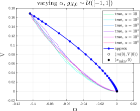
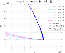
Figure 1. Plot of the solutions to systems (13)-(18) and (25) (with $\tilde{x}$ replaced by $x_{\textnormal{min}}$) in the phase space $(m,V)$ for several values of $\alpha$. On the right, zoom on a neighborhood of $(x_{\textnormal{min}},0)$.

In Figure 2, we fix $\alpha=10^{5}$ and choose two other initial conditions, in addition to $g_{X,0}\sim\mathcal{U}([-1,1])$ (identified by the color blue) of the previous figure. More precisely, we fix $g_{X,0}\sim\mathcal{U}([-0.2,0.5]),\mathcal{U}([-0.5,0.2])$, so to have $(m(0),V(0))$ spanning in both two upper quadrants. Once again, we notice a similar decay in both the true and approximated systems.

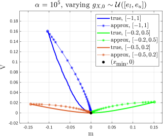
Figure 2. Plot of the solutions to systems (13)-(18) and (25) (with $\tilde{x}$ replaced by $x_{\textnormal{min}}$) in the phase space $(m,V)$ for three choices of initial data $g_{X,0}$.

Remark 4.2.

In Test 3, we couple the use of the stochastic Rastrigin function in one dimension ($d=1$) with parameters (34a). A comparison of these parameters with those used for the same objective in dimension $d=20$ from Tests 1 and 2 reveals that the values of $\sigma$ and $n_{\textnormal{it}}$ are lower. This choice reflects an interplay, already observed in previous works on CBO, between the dimension $d$ of the search space and the parameters $\sigma$ and $n_{\textnormal{it}}$. We refer to [43, 17] for more details concerning the tuning of the parameters.

5. Conclusion

We propose two procedures for solving an optimization problem where the cost function is given in the form of an expectation by a combination of variable-sample strategies and consensus-based algorithms and their kinetic generalization. We introduce CBO-FVSe, a time-discrete consensus-type algorithm in which the expected value is replaced at each time iterate by a suitable averaging. We show that its feature of generating independent estimates at different iterations leads to a reduction in the computational cost with respect to a recently introduced method for solving the same stochastic problem based on the sample average approximation theory. We assess its ability to capture the global minimizer numerically and provide a proof of convergence through a kinetic reinterpretation of the algorithm. We prove that the particle distribution satifies a time-continuous Boltzmann equation and use the evolution of its moment to prove convergence to the global minimum. We also investigate the stability of the solution involving the expected mean and variance, based on an assumption whose consistency we verify numerically.

With respect to the standard CBO and KBO, CBO-FVSe and KBO-FVSe require fixing two additional parameters, namely the sample size $M$ and the sampling distribution $\nu^{\overrightarrow{\mathbf{Y}}}$. In the sequel we plan to take up the original idea of variable-sample schemes, and extend the two procedures to the usage of a schedule of sample size $\{M_{h}\}_{h}$ and varying sampling distribution $\{\nu^{\overrightarrow{\mathbf{Y}}_{h}}\}_{h}$, so to improve the efficiency of the two methods proposed.

References

- [1] G. Albi, F. Ferrarese, and C. Totzeck. Kinetic based optimization enhanced by genetic dynamics. Preprint arXiv:2306.09199, 2023.
- [2] R. L. Anderson. Recent advances in finding best operating conditions. Journal of the American Statistical Association, 48(264):789–798, 1953.
- [3] H. Babovsky. On a simulation scheme for the Boltzmann equation. Mathematical Methods in the Applied Sciences, 8:223–233, 1986.
- [4] S. Bellavia and G. Malaspina. A discrete consensus-based global optimization method with noisy objective function. Preprint arXiv:2408.10078, 2024.
- [5] A. Benfenati, G. Borghi, and L. Pareschi. Binary interaction methods for high dimensional global optimization and machine learning. Applied Mathematics & Optimization, 86(1):9, 2022.
- [6] L. Bianchi, M. Birattari, M. Chiarandini, M. Manfrin, M. Mastrolilli, L. Paquete, O. Rossi-Doria, and T. Schiavinotto. Metaheuristics for the vehicle routing problem with stochastic demands. In Parallel Problem Solving from Nature-PPSN VIII: 8th International Conference, Birmingham, UK, September 18-22, 2004. Proceedings 8, pages 450–460. Springer, 2004.
- [7] L. Bianchi, M. Dorigo, L. M. Gambardella, and W. J. Gutjahr. A survey on metaheuristics for stochastic combinatorial optimization. Natural Computing, 8:239–287, 2009.
- [8] C. Blum and A. Roli. Metaheuristics in combinatorial optimization: overview and conceptual comparison. ACM computing surveys (CSUR), 35(3):268–308, 2003.
- [9] S. Bonandin and M. Herty. Consensus-based algorithms for stochastic optimization problems. Preprint arXiv:2404.10372, 2024.
- [10] G. Borghi, M. Herty, and L. Pareschi. A consensus-based algorithm for multi-objective optimization and its mean-field description. In 2022 IEEE 61st Conference on Decision and Control (CDC), pages 4131–4136. IEEE, 2022.
- [11] G. Borghi, M. Herty, and L. Pareschi. An adaptive consensus based method for multi-objective optimization with uniform Pareto front approximation. Applied Mathematics & Optimization, 88(2):58, 2023.
- [12] G. Borghi, M. Herty, and L. Pareschi. Constrained consensus-based optimization. SIAM Journal on Optimization, 33(1):211–236, 2023.
- [13] G. Borghi, M. Herty, and L. Pareschi. Kinetic models for optimization: a unified mathematical framework for metaheuristics. Preprint arXiv:2410.10369, 2024.
- [14] G. Borghi, H. Huang, and J. Qiu. A particle consensus approach to solving nonconvex-nonconcave min-max problems. Preprint arXiv:2407.17373, 2024.
- [15] J. A. Carrillo, Y. P. Choi, C. Totzeck, and O. Tse. An analytical framework for consensus-based global optimization method. Mathematical Models and Methods in Applied Sciences, 28(06):1037–1066, 2018.
- [16] J. A. Carrillo, F. Hoffmann, A. M. Stuart, and U. Vaes. Consensus-based sampling. Studies in Applied Mathematics, 148(3):1069–1140, 2022.
- [17] J. A. Carrillo, S. Jin, L. Li, and Y. Zhu. A consensus-based global optimization method for high dimensional machine learning problems. ESAIM: Control, Optimisation and Calculus of Variations, 27:S5, 2021.
- [18] J. A. Carrillo, S. Jin, H. Zhang, and Y. Zhu. An interacting particle consensus method for constrained global optimization. Preprint arXiv:2405.00891, 2024.
- [19] J. A. Carrillo, C. Totzeck, and U. Vaes. Consensus-based optimization and ensemble Kalman inversion for global optimization problems with constraints. In Modeling and Simulation for Collective Dynamics, pages 195–230. World Scientific, 2023.
- [20] C. Cercignani. The Boltzmann equation and its applications, volume 67. Springer Series in Applied Mathematical Sciences, 1988.
- [21] C. Cercignani, R. Illner, and M. Pulvirenti. The mathematical theory of dilute gases, volume 106. Springer Science & Business Media, 2013.
- [22] A. Dembo and O. Zeitouni. Large deviations techniques and applications, volume 38. Springer Science & Business Media, 2009.
- [23] F. Ferrarese and C. Totzeck. Localized KBO with genetic dynamics for multi-modal optimization. Preprint arXiv:2411.04840, 2024.
- [24] M. Fornasier, T. Klock, and K. Riedl. Convergence of anisotropic consensus-based optimization in mean-field law. In International Conference on the Applications of Evolutionary Computation (Part of EvoStar), pages 738–754. Springer, 2022.
- [25] M. Fornasier, T. Klock, and K. Riedl. Consensus-based optimization methods converge globally. SIAM Journal on Optimization, 4(3):973–3004, 2024.
- [26] M. Fornasier, L. Pareschi, H. Huang, and P. Suennen. Consensus-based optimization on the sphere: Convergence to global minimizers and machine learning. Journal of Machine Learning Research, 22(237):1–55, 2021.
- [27] N. García Trillos, A. Kumar Akash, S. Li, K. Riedl, and Y. Zhu. Defending against diverse attacks in federated learning through consensus-based bi-level optimization. Preprint arXiv:2412.02535, 2024.
- [28] N. García Trillos, S. Li, K. Riedl, and Y. Zhu. CB2O: Consensus-based bi-level optimization. Preprint arXiv:2411.13394, 2024.
- [29] W. J. Gutjahr. A converging ACO algorithm for stochastic combinatorial optimization. In Stochastic Algorithms: Foundations and Applications: Second International Symposium, SAGA 2003, Hatfield, UK, September 22-23, 2003. Proceedings 2, pages 10–25. Springer, 2003.
- [30] W. J. Gutjahr. S-ACO: An ant-based approach to combinatorial optimization under uncertainty. In International Workshop on Ant Colony Optimization and Swarm Intelligence, pages 238–249. Springer, 2004.
- [31] S.-Y. Ha, S. Jin, and D. Kim. Convergence of a first-order consensus-based global optimization algorithm. Mathematical Models and Methods in Applied Sciences, 30(12):2417–2444, 2020.
- [32] S.-Y. Ha, S. Jin, and D. Kim. Convergence and error estimates for time-discrete consensus-based optimization algorithms. Numerische Mathematik, 147:255–282, 2021.
- [33] D. J. Higham. An algorithmic introduction to numerical simulation of stochastic differential equations. SIAM review, 43(3):525–546, 2001.
- [34] M.W. Hirsch, S. Smale, and R. L. Devaney. Differential equations, dynamical systems, and an introduction to chaos. Academic press, 2013.
- [35] T. Homem-de Mello. Variable-sample methods and simulated annealing for discrete stochastic optimization. Stochastic Programming E-Print Series, Humboldt-Universität zu Berlin, 2000.
- [36] T. Homem-De-Mello. Variable-sample methods for stochastic optimization. ACM Transactions on Modeling and Computer Simulation (TOMACS), 13(2):108–133, 2003.
- [37] H. Huang, J. Qiu, and K. Riedl. Consensus-based optimization for saddle point problems. SIAM Journal on Control and Optimization, 62(2):1093–1121, 2024.
- [38] M. Jamil and X.S. Yang. A literature survey of benchmark functions for global optimisation problems. International Journal of Mathematical Modelling and Numerical Optimisation, 4(2):150–194, 2013.
- [39] D. Ko, S.Y. Ha, S. Jin, and D. Kim. Convergence analysis of the discrete consensus-based optimization algorithm with random batch interactions and heterogeneous noises. Mathematical Models and Methods in Applied Sciences, 32(06):1071–1107, 2022.
- [40] K. Nanbu. Direct simulation scheme derived from the Boltzmann equation. I. Monocomponent gases. Journal of the Physical Society of Japan, 49(5):2042–2049, 1980.
- [41] V. I. Norkin, Y. M. Ermoliev, and A. Ruszczyński. On optimal allocation of indivisibles under uncertainty. Operations Research, 46(3):381–395, 1998.
- [42] L. Pareschi and G. Russo. An introduction to Monte Carlo methods for the Boltzmann equation. In ESAIM: Proceedings, volume 10, pages 35–75. EDP Sciences, 2001.
- [43] R. Pinnau, C. Totzeck, O. Tse, and S. Martin. A consensus-based model for global optimization and its mean-field limit. Mathematical Models and Methods in Applied Sciences, 27(01):183–204, 2017.
- [44] J. Schneider and S. Kirkpatrick. Stochastic optimization. Springer Science & Business Media, 2006.
- [45] A. Shapiro. Monte Carlo sampling methods. Handbooks in operations research and management science, 10:353–425, 2003.
- [46] A. Shapiro, D. Dentcheva, and A. Ruszczynski. Lectures on stochastic programming: modeling and theory. SIAM, 2021.
- [47] J. C. Spall. Introduction to stochastic search and optimization: estimation, simulation, and control. John Wiley & Sons, 2005.
- [48] G. Toscani. Kinetic models of opinion formation. Communications in Mathematical Sciences, 4(3):481–496, 2006.
- [49] C. Totzeck. Trends in consensus-based optimization. In Active Particles, Volume 3: Advances in Theory, Models, and Applications, pages 201–226. Springer, 2021.
- [50] F. Verhulst. Nonlinear differential equations and dynamical systems. Springer Science & Business Media, 2012.