Model-Free Adversarial Purification via Coarse-To-Fine Tensor Network Representation

Abstract

Deep neural networks are known to be vulnerable to well-designed adversarial attacks. Although numerous defense strategies have been proposed, many are tailored to the specific attacks or tasks and often fail to generalize across diverse scenarios. In this paper, we propose Tensor Network Purification (TNP), a novel model-free adversarial purification method by a specially designed tensor network decomposition algorithm. TNP depends neither on the pre-trained generative model nor the specific dataset, resulting in strong robustness across diverse adversarial scenarios. To this end, the key challenge lies in relaxing Gaussian-noise assumptions of classical decompositions and accommodating the unknown distribution of adversarial perturbations. Unlike the low-rank representation of classical decompositions, TNP aims to reconstruct the unobserved clean examples from an adversarial example. Specifically, TNP leverages progressive downsampling and introduces a novel adversarial optimization objective to address the challenge of minimizing reconstruction error but without inadvertently restoring adversarial perturbations. Extensive experiments conducted on CIFAR-10, CIFAR-100, and ImageNet demonstrate that our method generalizes effectively across various norm threats, attack types, and tasks, providing a versatile and promising adversarial purification technique.

1 Introduction

Deep neural networks (DNNs) have achieved remarkable success across a wide range of tasks. However, DNNs have been shown to be vulnerable to adversarial examples (Szegedy et al., 2014; Goodfellow et al., 2015), which are generated by adding small, human-imperceptible perturbations to natural images but completely change the prediction results to DNNs, leading to disastrous implications. The vulnerability of DNNs to such examples highlights the significance of robust defense mechanisms to mitigate adversarial attacks effectively.

Since then, numerous methods have been proposed to defend against adversarial examples. Notably, adversarial training (AT, Goodfellow et al., 2015) typically aims to retrain DNNs using adversarial examples, achieving robustness over seen types of adversarial attacks but performing poorly against unseen perturbations (Laidlaw et al., 2021; Dolatabadi et al., 2022). Another class of defense methods is adversarial purification (AP, Yoon et al., 2021), which leverages pre-trained generative models to remove adversarial perturbations and demonstrates better generalization than AT against unseen attacks (Nie et al., 2022; Lin et al., 2024). However, AP methods rely on pre-trained models tailored to specific datasets, limiting their transferability to different data distributions and tasks. Thus, both mainstream techniques face generalization challenges: AT struggles with diverse norm threats, and AP with task generalization, restricting their applicability to broader scenarios.

To tackle these challenges, we propose a novel model-free adversarial purification method by a specially designed tensor network decomposition algorithm, termed Tensor Network Purification (TNP), which bridges the gap between low-rank tensor network representation with Gaussian noise assumption and removal of adversarial perturbations with unknown distributions. As a model-free optimization technique (Oseledets, 2011; Zhao et al., 2016), TNP depends neither on any pre-trained generative model nor specific dataset, enabling it to achieve strong robustness across diverse adversarial scenarios. Additionally, TNP can eliminate potential adversarial perturbations for both clean or adversarial examples before feeding them into the classifier (Yoon et al., 2021). As a pre-processing step, TNP can defend against adversarial attacks without retraining the classifier model or pretraining the generative model. Moreover, since our method is an algorithm applied to input examples only and has no fixed model parameters, it is more difficult to be attacked by existing black or white box adversarial attack techniques. Consequently, benefiting from the aforementioned advantages, it is evident that TN-based AP methods represent a highly promising direction, offering the transferability to be effectively applied across a wide range of adversarial scenarios.

The existing TN methods are particularly favorable for image completion and denoising when the noise is sparse or follows Gaussian distribution as long as it can be modeled explicitly. However, the distribution of well-designed adversarial perturbations fundamentally differs from such noises and often aligns with the statistics of the data (Ilyas et al., 2019; Allen-Zhu & Li, 2022). Consequently, these perturbations behave more like features than noise, making them challenging to be modeled explicitly and prone to being inadvertently reconstructed. To address this issue, we first explore the distribution changes of perturbations during the optimization process and initially mitigate the impact of perturbations by progressive downsampling. Correspondingly, we propose an algorithm for TN incremental learning in a coarse-to-fine manner. Furthermore, a novel adversarial optimization objective is proposed to address the challenge of minimizing reconstruction error but without inadvertently restoring adversarial perturbations. Unlike classical TN, given an adversarial example, TNP prevents naive low-rank representation of the input and encourages the reconstructed examples to approximate the unobserved clean examples.

We empirically evaluate the performance of our method by comparing it with AT and AP methods across attack settings using multiple classifier models on CIFAR-10, CIFAR-100, and ImageNet. The results demonstrate that our method achieves state-of-the-art performance with robust generalization across diverse adversarial scenarios. Specifically, our method achieved a 26.45% improvement in average robust accuracy over AT across different norm threats, a 9.39% improvement over AP across multiple attacks, and a 6.47% improvement over AP across different datasets. Furthermore, in denoising tasks, our method effectively removes adversarial perturbations while preserving consistency between the reconstructed clean example and the reconstructed adversarial example. These results collectively underscore the effectiveness and potential of our proposed method. In summary, our contributions are as follows:

• We introduce a model-free adversarial purification framework based on tensor network representation, which eliminates the need for training a powerful generative model or relying on specific dataset distributions, making it a general-purpose adversarial purification.

• Based on our analysis of the distribution changes of adversarial perturbations during optimization, we propose a novel adversarial optimization objective for coarse-to-fine TN representation learning to prevent the restoration of adversarial perturbations.

• We conduct extensive experiments on various datasets, demonstrating that our method achieves state-of-the-art performance, especially exhibiting robust generalization across diverse adversarial scenarios.

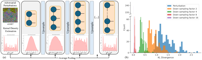
Figure 1: Compare the adversarial perturbations in the downsampled images. (a) The distribution changes of adversarial perturbations during downsampling process. More results are shown in Appendix G. (b) The KL divergence histogram of adversarial perturbations.

2 Related Works

Adversarial robustness  To defend against adversarial attacks, researchers have developed various techniques aimed at enhancing the robustness of DNNs. Goodfellow et al. (2015) propose AT technique to defend against adversarial attacks by retraining classifiers using adversarial examples. In contrast, AP methods (Shi et al., 2021; Srinivasan et al., 2021) aim to purify adversarial examples before classification without retraining the classifier. Currently, the most common AP methods (Nie et al., 2022; Bai et al., 2024) rely on pre-trained generative models as purifiers, which are trained on specific datasets and hard to generalize to data distributions outside their training domain. Lin et al. (2024) propose applying AT technique to AP, optimizing the purifier to adapt to new data distributions. Although our framework employs AP strategy, it fundamentally deviates from these works as we develop a model-free framework that relies solely on the information of the input example for adversarial purification, without requiring any additional priors from pre-trained models or training the purifiers.

Tensor network and TN-based defense methods  Tensor network (TN) is a classical tool in signal processing, with many successful applications in image completion and denoising (Kolda & Bader, 2009; Cichocki et al., 2015). Compared to traditional TN methods such as TT (Oseledets, 2011) and TR (Zhao et al., 2016), we employ the quantized technique (Khoromskij, 2011) and develop a coarse-to-fine strategy. Recently, PuTT (Loeschcke et al., 2024) also employs a coarse-to-fine strategy, aiming to achieve better initialization for faster and more efficient TT decomposition by minimizing the reconstruction error. In comparison, our method progresses from low to high resolution, explicitly targeting perturbation removal and analyzing the impact of downsampling on perturbations. Furthermore, we propose a novel optimization objective that goes beyond simply minimizing the reconstruction error, focusing instead on preventing the reappearance of adversarial perturbations.

With the growing concern over adversarial robustness, a line of work has attempted to leverage TNs as robust denoisers to defend against adversarial attacks. In particular, Yang et al. (2019) reconstruct images and retrain classifiers to adapt to the new reconstructed distribution. Entezari & Papalexakis (2022) analyze vanilla TNs and show their effectiveness in removing high-frequency perturbations. Additionally, (Bhattarai et al., 2023) extend the application of TNs beyond data to include classifiers, a concept similar to the approaches of (Rudkiewicz et al., 2024; Phan et al., 2023). Furthermore, (Song et al., 2024) employ training-free techniques while incorporating ground truth information to defend against adversarial attacks. However, the aforementioned methods rely on additional prior or are limited to specific attacks. In this paper, we aim to achieve robustness solely by optimizing TNs themselves, establishing them as a plug-and-play and promising adversarial purification technique.

3 Backgrounds

Notations  Throughout the paper, we denote scalars, vectors, matrices, and tensors as lowercase letters, bold lowercase letters, bold capital letters, and calligraphic bold capital letters, e.g., $x$, $\boldsymbol{x}$, $\boldsymbol{X}$ and $\boldsymbol{\mathcal{X}}$, respectively. A $D$-order tensor tensor is an $D$-dimensional array, e.g., a vector is a 1st-order tensor and a matrix is a 2nd-order tensor. For a $D$-order tensor $\boldsymbol{\mathcal{X}}\in\mathbb{R}^{I_{1}\times\dots\times I_{D}}$, we denote its ($i_{1},\dots,i_{D}$)-th entry as $x_{\mathbf{i}}$, where $\mathbf{i}=$ ($i_{1},\dots,i_{D}$). Following the conventions in deep learning, we treat images as vectors, e.g., input example $\boldsymbol{x}_{in}$, clean example $\boldsymbol{x}_{cln}$, adversarial example $\boldsymbol{x}_{adv}$ and reconstructed example $\boldsymbol{y}$.

Tensor network decomposition  Given a $D$-order tensor $\boldsymbol{\mathcal{X}}\in\mathbb{R}^{I_{1}\times\ldots\times I_{D}}$, tensor network decomposition factorizes $\boldsymbol{\mathcal{X}}$ into $D$ smaller latent components by using some predefined tensor contraction rules. Among tensor network decompositions, Tensor Train (TT) decomposition (Oseledets, 2011) enjoys both quasi-optimal approximation as well as the high compression rate of large and complex data tensors. In particular, a $D$-order tensor $\boldsymbol{\mathcal{X}}\in\mathbb{R}^{I_{1}\times\ldots\times I_{D}}$ has the TT format as ${x}_{\mathbf{i}}=\boldsymbol{A}^{1}_{i_{1}}\boldsymbol{A}^{2}_{i_{2}}\ldots\boldsymbol{A}^{D}_{i_{D}}\,,$ where $\boldsymbol{A}^{d}_{i_{d}}\in\mathbb{R}^{r_{d-1}\times r_{d}}$, for $d\in[D]$ and $i_{d}\in[I_{d}]$. Then, $(1,r_{1},\ldots,r_{d-1},1)$ is the TT rank of $\boldsymbol{\mathcal{X}}$. For simplicity, we denote $\boldsymbol{\mathcal{X}}=\text{TT}(\boldsymbol{\mathcal{A}}^{1},\ldots,\boldsymbol{\mathcal{A}}^{D})$. When each dimension $I_{d}$ of $\boldsymbol{\mathcal{X}}$ is large, quantized tensor train (QTT, Khoromskij, 2011) becomes highly efficient, which splits each dimension in powers of two. For example, a $2^{D}\times 2^{D}$ image can be rearranged into a more expressive and balanced $D$-order tensor. For brevity, hereafter, a $2^{D}\times 2^{D}$ image $\boldsymbol{x}_{D}$ shall be called a resolution $D$ image, whose quantized tensor is $\boldsymbol{\mathcal{X}}_{D}=\operatorname{Q}(\boldsymbol{x}_{D})$.

4 Method

Tensor network (TN) is a classical tool in signal processing, with many successful applications in image completion and denoising. By leveraging the $\ell_{2}$-norm as the primary optimization criterion, which aligns well with the statistical properties of a normal distribution, these methods (Phan et al., 2020; Loeschcke et al., 2024) have demonstrated strong capabilities in removing Gaussian noise.

However, the distribution of well-designed adversarial perturbations is essentially different from Gaussian noise and cannot be modeled explicitly (Ilyas et al., 2019; Allen-Zhu & Li, 2022), thereby challenging the conventional assumptions of TN-based denoising methods, leading to ineffectiveness on adversarial purification for $\boldsymbol{x}_{adv}$. To minimize the loss $\|\boldsymbol{x}_{adv}-\text{TN}(\boldsymbol{x}_{adv})\|_{2}$, TN decompositions fit all feature components of $\boldsymbol{x}_{adv}$, including the adversarial perturbations. However, in the presence of adversarial attacks, we aim to restore unobserved $\boldsymbol{x}_{cln}$ from the input $\boldsymbol{x}_{adv}$, that is: $\text{TN}(\boldsymbol{x}_{adv})\approx\boldsymbol{x}_{cln}$ rather than $\boldsymbol{x}_{adv}$.

Based on the above analysis, it is crucial to overcome two challenges in designing an effective TN method:

Q1. How can we transform the distribution of non-specific perturbations into well-known distributions?

Q2. How can we avoid overly constraints of reconstruction error from inadvertently restoring those perturbations?

To address these two issues, we explore how adversarial perturbations evolve when using average pooling as downsampling. Intuitively, the central limit theorem suggests that as an image is progressively downsampled, aggregated perturbations begin to resemble a normal distribution. Thus, even an $\ell_{2}$-based penalty becomes effective in suppressing the perturbations at lower resolutions.

However, while this insight helps suppress perturbations at lower resolutions, there remains the challenge of reconstructing the full-resolution image. When upsampling and further optimizing using $\|\boldsymbol{x}_{adv}-\text{TN}(\boldsymbol{x}_{adv})\|_{2}$, the perturbations will still be restored. This connects with our second question, for which we design a new optimization objective.

4.1 Downsampling using average pooling

An intuitive explanation for why downsampling aids in perturbation removal can be derived from the Central Limit Theorem (CLT, Grzenda & Zieba, 2008). When an image is downsampled by average pooling, the random components (e.g., pixel-level noise or minor adversarial perturbations) within those pooling patches are aggregated. We hypothesize that, given an adversarial example $\boldsymbol{x}_{adv}$, downsampling the $\boldsymbol{x}_{adv}$ from its original resolution $D$ to a lower resolution $D-1$ will smooth out the adversarial perturbations. As the downsampling process progresses further, the distribution of the aggregated adversarial perturbations in the low-resolution image $\boldsymbol{x}_{D-l}$ is expected to converge toward a normal distribution, as illustrated in Figure 1a.

To investigate this hypothesis in real datasets, we compute the KL divergence between the histograms of adversarial perturbations and the Gaussian distributions with the same sample mean and variance across 512 images from ImageNet. As shown in Figure 1b, the distribution of those perturbations progressively aligns with that of Gaussian noise as the downsampling process progresses. Additionally, to further support our hypothesis of using the average pooling, we compare the influence of different downsampling methods, as discussed in Appendix A.

4.2 Tensor network purification

Building upon our downsampling-based intuition, we design a coarse-to-fine process and adopt PuTT (Loeschcke et al., 2024) as our base model, which employs progressive downsampling for better initialization of QTT cores. The workflow of tensor network purification (TNP) for classification tasks is illustrated in Figure 2, where the quantized $\boldsymbol{\mathcal{X}}=\operatorname{Q}(\boldsymbol{x})$, TT decomposition $\boldsymbol{\mathcal{X}}\approx\boldsymbol{\mathcal{Y}}=\text{TT}(\boldsymbol{\mathcal{A}}^{1},\ldots,\boldsymbol{\mathcal{A}}^{D})$, and reconstruction $\boldsymbol{y}=\operatorname{Q}^{-1}(\boldsymbol{\mathcal{Y}})$ processes are depicted.

Initially, the $2^{D}\times 2^{D}$ input example $\boldsymbol{x}_{D}$ (potentially adversarial example $\boldsymbol{x}_{adv}$ or clean example $\boldsymbol{x}_{cln}$), whose quantized version is a $D$-order tensor $\boldsymbol{\mathcal{X}}_{D}$, is first downsampled to a resolution $D-l$ example $\boldsymbol{x}_{D-l}$, corresponding to a $(D-l)$-order tensor $\boldsymbol{\mathcal{X}}_{D-l}$. The QTT cores of $\boldsymbol{\mathcal{X}}_{D-l}$ are optimized by PuTT via backpropagation within a standard reconstruction error $||\boldsymbol{x}_{D-l}-\boldsymbol{y}_{D-l}||_{2}$. Once the approximation of $\boldsymbol{\mathcal{X}}_{D-l}$ is stabilized, the prolongation operator $\boldsymbol{\mathcal{P}}_{D-l+1}$ is applied to the QTT format of $\boldsymbol{\mathcal{X}}_{D-l}$, producing a $(D-l+1)$-order tensor $\boldsymbol{\mathcal{P}}_{D-l+1}\boldsymbol{\mathcal{X}}_{D-l}$. Additionally, we define the linear function $\text{P}_{d}(\cdot)$ acts on the image level, with the effect of upsampling from resolution $d-1$ to $d$, details in Section B.2. This serves as an initialization to find the optimal QTT cores of $\boldsymbol{\mathcal{X}}_{D-l+1}$ and reconstructed downsampled example $\boldsymbol{y}_{D-l}$.

Next, the input example $\boldsymbol{x}_{D}$ is once again downsampled to a resolution $D-l+1$ example $\boldsymbol{x}_{D-l+1}$. However, this time, the QTT cores of $\boldsymbol{\mathcal{X}}_{D-l+1}$ are optimized using the adversarial optimization objective within a novel loss function as shown in Eq. 1. Similarly, once the approximation of $\boldsymbol{\mathcal{X}}_{D-l+1}$ stabilizes, the upsampling operation is performed. This process is repeated iteratively until reaching the QTT approximation $\boldsymbol{\mathcal{Y}}_{D}$ of the original resolution $\boldsymbol{\mathcal{X}}_{D}$.

Finally, tensor network purification (TNP) can purify the potential adversarial examples ($\boldsymbol{x}_{cln}$ or $\boldsymbol{x}_{adv}$) before feeding them into the classifier model $f$, e.g., $f(\text{TNP}(\boldsymbol{x}_{cln}))=f(\text{TNP}(\boldsymbol{x}_{adv}))=y$, where $y$ is the ground truth. As a plug-and-play module, TNP can be integrated with any classifiers.

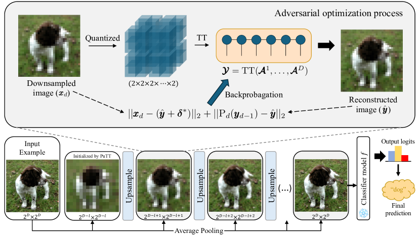
Figure 2: Illustration of tensor network purification.

4.3 Adversarial optimization process

Following the coarse-to-fine process, despite the downsampling with average pooling and subsequent PuTT at lower resolutions can mitigate adversarial perturbations, the other challenge arises upon reconstructing the example at the original resolution, where minimizing standard reconstruction error will inevitably restore those perturbations.

Algorithm 1 Adversarial optimization process.

 Input: Example $\boldsymbol{x}_{d}$, number of iterations $T$, inner maximization steps $N$, scale $\alpha$ and $\eta$, learning rate $\beta$

 Output: Reconstructed examples $\boldsymbol{y}_{d}$

 Initialize $\hat{\boldsymbol{y}}\leftarrow\text{P}_{d}(\boldsymbol{y}_{d-1})$

 for $t=1,2,\dots,T$ do

  Initialize $\boldsymbol{\delta}\leftarrow\boldsymbol{0}$

  for $n=1,2,\dots,N$ do

   $\ell\leftarrow\mathcal{L}_{adv}(\hat{\boldsymbol{y}}+\boldsymbol{\delta},\boldsymbol{x}_{d})$

   $\boldsymbol{\delta}\leftarrow\text{clip}(\boldsymbol{\delta}+\alpha\text{sign}(\nabla_{\hat{\boldsymbol{y}}}\ell),-\eta,\eta)$

  end for

  $\boldsymbol{\delta}^{*}\leftarrow\text{clip}(\hat{\boldsymbol{y}}+\boldsymbol{\delta},0,1)-\hat{\boldsymbol{y}}$

  Gradient descent based on loss in Eq. 1:

  $\hat{\boldsymbol{y}}\leftarrow\hat{\boldsymbol{y}}-\beta\nabla_{\hat{\boldsymbol{y}}}\mathcal{L}$

 end for

 return $\boldsymbol{y}_{d}\leftarrow\hat{\boldsymbol{y}}$

Unlike traditional reconstruction tasks, in the context of adversarial attacks, we can only observe the adversarial example $\boldsymbol{x}_{adv}$, while the goal is to reconstruct a “clean” version $\boldsymbol{y}$ closing to the unobserved clean example $\boldsymbol{x}_{cln}$. To bridge the gap between $\boldsymbol{x}_{adv}$ and $\boldsymbol{x}_{cln}$, we propose a new optimization objective that introduces an auxiliary variable $\boldsymbol{\delta}$ by inner maximization. Additionally, we leverage a reconstructed downsampled example as a crucial prior to guide the approximation toward $\boldsymbol{x}_{cln}$.

Here, we outline the optimization procedure for $x_{d}$, which corresponds to the gray box in Figure 2. Formally, given the resolution $d$ example $\boldsymbol{x}_{d}$, we attempt to obtain the reconstructed example $\boldsymbol{y}_{d}$ by performing gradient descent on optimization loss functions of

$$\mathcal{L}(\boldsymbol{x}_{d},\hat{\boldsymbol{y}},\boldsymbol{\delta}^{*}) =||\boldsymbol{x}_{d}-(\hat{\boldsymbol{y}}+\boldsymbol{\delta}^{*})||_{2}+||\text{P}_{d}(\boldsymbol{y}_{d-1})-\hat{\boldsymbol{y}}||_{2},$$ (1)

$$\text{s.t. }\boldsymbol{\delta}^{*} =\arg\max_{\lVert\boldsymbol{\delta}\rVert<\eta}\mathcal{L}_{adv}(\hat{\boldsymbol{y}}+\boldsymbol{\delta},\boldsymbol{x}_{d}),$$

where $d\in[D-l+1,D]$ and $\eta$ is a scale hyperparameter.

The auxiliary variable $\boldsymbol{\delta}^{*}$ is determined through an inner maximization process that utilizes a non-convex loss function $\mathcal{L}_{adv}$. We employ a perceptual metric, structural similarity index measure (SSIM, Hore & Ziou, 2010), as $\mathcal{L}_{adv}$ to explore more potential solutions and better handle complex perturbation patterns. While $\boldsymbol{\delta}^{*}$ does not exactly represent the true adversarial perturbation, bounding $\lVert\boldsymbol{\delta}\rVert<\eta$ can partially ensure that the misalignment between $\boldsymbol{y}$ and $\boldsymbol{x}_{adv}$ remains controlled, effectively ensuring that $\boldsymbol{y}$ does not simply collapse into the adversarial example $\boldsymbol{x}_{adv}$.

However, also since $\boldsymbol{\delta}^{*}$ does not represent the true perturbation, minimizing $||\boldsymbol{x}_{d}-(\hat{\boldsymbol{y}}+\boldsymbol{\delta}^{*})||_{2}$ may not yield the desired clean reconstructed example. To address this limitation, we introduce a second loss term $||\text{P}_{d}(\boldsymbol{y}_{d-1})-\hat{\boldsymbol{y}}||_{2}$. Specifically, we utilize the reconstructed downsampled example $\boldsymbol{y}_{d-1}$ as an additional prior constraint to aid in approximating the $\boldsymbol{x}_{cln})$. Building upon the observations in Figure 1, we start from the resolution $D-l$ example $\boldsymbol{x}_{D-l}$, optimized by PuTT, and then perform upsampling to the higher resolution to produce a “clean-leaning” reference, which nudges $\boldsymbol{y}$ toward a less perturbed distribution. Although the clean example $\boldsymbol{x}_{cln}$ cannot be obtained as a prior for the optimization, we devise a clever way to provide a surrogate prior and guide the optimization process. The detailed algorithm of our adversarial optimization process is shown in Algorithm 1.

5 Experiments

In this section, we conduct extensive experiments on CIFAR-10, CIFAR-100, and ImageNet across various attack settings to evaluate the performance of our method. The classification results demonstrate that the proposed method achieves state-of-the-art performance and exhibits strong generalization capabilities. Specifically, our method achieved a 26.45% improvement in average robust accuracy over AT across different norm threats, a 9.39% improvement over AP across multiple attacks, and a 6.47% improvement over AP across different datasets. Next, we investigate the effectiveness of adversarial perturbation removal in denoising tasks using the existing tensor network decomposition methods. Among these, only our method successfully removes adversarial perturbations while preserving consistency between the reconstructed clean example and the reconstructed adversarial example. These results collectively highlight the effectiveness and potential of our proposed method.

5.1 Experimental setup

Datasets and model architectures  We conduct extensive experiments on CIFAR-10, CIFAR-100 (Krizhevsky et al., 2009) and ImageNet (Deng et al., 2009) to empirically validate the effectiveness of the proposed methods against adversarial attacks. For classification tasks, we utilize the pre-trained ResNet (He et al., 2016) and WideResNet (Zagoruyko & Komodakis, 2016) models. For denoising tasks, we employ Tensor Train (TT, Oseledets, 2011), Tensor Ring (TR, Zhao et al., 2016), quantized technique (Khoromskij, 2011) and PuTT (Loeschcke et al., 2024).

Adversarial attacks  We evaluate our method against AutoAttack (Croce & Hein, 2020), a widely used benchmark that integrates both white-box and black-box attacks. Additionally, following the guidance of Lee & Kim (2023), we utilize projected gradient descent (PGD, Madry et al., 2018) with expectation over time (EOT, Athalye et al., 2018) for a more comprehensive evaluation.

Due to the high computational cost of evaluating methods with multiple attacks, following the guidance of Nie et al. (2022), we randomly select 512 images from the test set for robust evaluation. All experiments presented in the paper are conducted by NVIDIA RTX A5000 with 24GB GPU memory, CUDA v11.7 and cuDNN v8.5.0 in PyTorch v1.13.11 (Paszke et al., 2019). More details in Appendix C.

5.2 Comparison with the state-of-the-art methods

Table 1: Standard and robust accuracy against AutoAttack $l_{\infty}$ threat ($\epsilon=8/255$) on CIFAR-10. (${}^{\text{\textdagger}}$the methods use additional synthetic images. ^∗use robust classifer (Cui et al., 2024).)

Defense method	Extra	Standard	Robust
	data	Acc.	Acc.
Zhang et al. (2020)	✓	85.36	59.96
Gowal et al. (2020)	✓	89.48	62.70
Bai et al. (2023)	$\checkmark^{\text{\textdagger}}$	95.23	68.06
Rebuffi et al. (2021)	$\times^{\text{\textdagger}}$	87.33	61.72
Gowal et al. (2021)	$\times^{\text{\textdagger}}$	88.74	66.11
Wang et al. (2023)	$\times^{\text{\textdagger}}$	93.25	70.69
Peng et al. (2023)	$\times^{\text{\textdagger}}$	93.27	71.07
Cui et al. (2024)	$\times^{\text{\textdagger}}$	92.16	67.73
Nie et al. (2022)	$\times$	89.02	70.64
Wang et al. (2022)	$\times$	84.85	71.18
Zhang et al. (2024)	$\times$	90.04	73.05
Lin et al. (2024)	$\times$	90.62	72.85
Ours	$\times$	82.23	55.27
Ours∗	$\times$	91.99	72.85

Table 2: Standard and robust accuracy against AutoAttack $l_{2}$ threat ($\epsilon=0.5$) on CIFAR-10. (${}^{\text{\textdagger}}$the methods use additional synthetic images. ^∗use robust classifer (Cui et al., 2024).)

Defense method	Extra	Standard	Robust
	data	Acc.	Acc.
Augustin et al. (2020)	✓	92.23	77.93
Gowal et al. (2020)	✓	94.74	80.53
Rebuffi et al. (2021)	$\times^{\text{\textdagger}}$	91.79	78.32
Ding et al. (2019)	$\times$	88.02	67.77
Nie et al. (2022)	$\times$	91.03	78.58
Ours	$\times$	82.23	68.16
Ours∗	$\times$	91.99	79.49

Table 3: Standard and robust accuracy against AutoAttack $l_{\infty}$ threat ($\epsilon=8/255$) on CIFAR-100 using WideResNet-28-10 classifier. (${}^{\text{\textdagger}}$the methods use additional synthetic images.)

Defense method	Extra	Standard	Robust
	data	Acc.	Acc.
Hendrycks et al. (2019)	✓	59.23	28.42
Debenedetti et al. (2023)	✓	70.76	35.08
Cui et al. (2024)	$\times^{\text{\textdagger}}$	73.85	39.18
Wang et al. (2023)	$\times^{\text{\textdagger}}$	75.22	42.67
Pang et al. (2022)	$\times$	63.66	31.08
Jia et al. (2022)	$\times$	67.31	31.91
Cui et al. (2024)	$\times$	65.93	32.52
Ours	$\times$	62.30	44.34

Table 4: Standard and robust accuracy against AutoAttack $l_{\infty}$ threat ($\epsilon=4/255$) on ImageNet using ResNet-50 classifier.

Defense method	Extra	Standard	Robust
	data	Acc.	Acc.
Engstrom et al. (2019)	$\times$	62.56	31.06
Wong et al. (2020)	$\times$	55.62	26.95
Salman et al. (2020)	$\times$	64.02	37.89
Bai et al. (2021)	$\times$	67.38	35.51
Nie et al. (2022)	$\times$	67.79	40.93
Chen & Lee (2024)	$\times$	68.76	40.60
Ours	$\times$	65.43	42.77

In this section, we evaluate our method for defending against AutoAttack $l_{\infty}$ and $l_{2}$ threats (Croce & Hein, 2020; Croce et al., 2021) and compare it with the state-of-the-art methods under all adversarial settings listed in RobustBench. Tables 1, 2, 3 and 4 present the performance of various defense methods against AutoAttack $l_{\infty}$ ($\epsilon=8/255$) and $l_{2}$ ($\epsilon=0.5$) threats on CIFAR-10, CIFAR-100 and ImageNet datasets. Overall, the highest robust accuracy achievable by our method is generally on par with the current state-of-the-art methods without using extra data (the dataset introduced by Carmon et al. (2019)). Specifically, compared to the second-best method, our method improves the robust accuracy by 1.67% on CIFAR-100, by 1.84% on ImageNet, and the average robust accuracy by 0.36% on CIFAR-10.

However, due to the overfitting of WideResNet-28-10 trained on the limited data available in CIFAR-10, we observe that the results of Ours struggle to reach state-of-the-art performance, consistent with findings from other AT methods. To address this issue, these methods incorporate additional synthetic data to train a robust classifier. Following this, we conduct experiments using the robust classifier trained by Cui et al. (2024), which utilizes an additional 20M synthetic images in training. This leads to a significant improvement in the robust accuracy observed in $\text{Ours}^{*}$. Moreover, compared to the used robust classifier, our method futher improves the robust accuracy by 5.12%. These results are consistent across multiple datasets and norm threats, confirming the effectiveness of our method and its potential for defending against adversarial attacks.

5.3 Generalization comparison across various scenarios

As previously mentioned, the existing defense methods are often criticized for their lack of generalization across different norm threats, attacks, and datasets. In this section, we evaluate the performance of our method under various settings to demonstrate its generalization capability.

Table 5: Standard accuracy (SA) and robust accuracy (RA) against AutoAttack $l_{\infty}$ ($\epsilon=8/255$) threat on CIFAR-10 and CIFAR-100 with WideResNet-28-10 classifier. The pre-trained generative model used in AP is trained on CIFAR-10.

Defense method	CIFAR-10		CIFAR-100		Avg.
	SA	RA	SA	RA	SA	RA
Standard Training	94.78	0.00	81.86	0.00	88.32	0.00
AT (Cui et al., 2024)	92.16	67.73	73.85	39.18	83.01	53.46
AP (Nie et al., 2022)	89.02	70.64	38.09	33.79	63.56	52.22
Ours∗	91.99	72.85	71.48	44.53	81.74	58.69

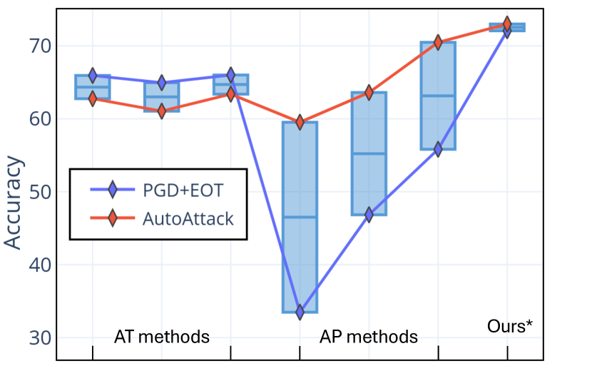
Figure 3: Comparison of robust accuracy against PGD+EOT and AutoAttack.

Results analysis on different norm-threats: Table 6 shows that AT methods (Laidlaw et al., 2021; Dolatabadi et al., 2022) are limited in defending against unseen attacks and can only effectively against the specific attacks they are trained on. The intuitive idea is to apply AT across all norm threats or develop more general constraints to obtain a robust model. However, training such a model is challenging due to the inherent differences among various attacks. In contrast, AP methods (Nie et al., 2022; Lin et al., 2024) exhibit strong generalization, effectively defending against unseen attacks. The results demonstrate that our method also possesses strong generalization capabilities against unseen attacks, achieving performance close to the state-of-the-art AP methods while significantly outperforming the existing AT methods. Specifically, compared to the best AT method, our method improves average robust accuracy by 26.45%.

Table 6: Standard accuracy and robust accuracy against AutoAttack $l_{\infty}$ ($\epsilon=8/255$) and AutoAttack $l_{2}$ ($\epsilon=1.0$) threats on CIFAR-10 with standard ResNet-50 classifier.

Type	Defense method	SA	Robust Acc.
			AA $l_{\infty}$	AA $l_{2}$
	Standard Training	94.8	0.0	0.0
AT	Training with $l_{\infty}$	86.8	49.0	19.2
	Training with $l_{2}$	85.0	39.5	47.8
	Laidlaw et al. (2021)	82.4	30.2	34.9
	Dolatabadi et al. (2022)	83.2	40.0	33.9
AP	Nie et al. (2022)	88.2	70.0	70.9
	Lin et al. (2024)	89.1	71.2	73.4
	Ours	88.3	73.2	67.0

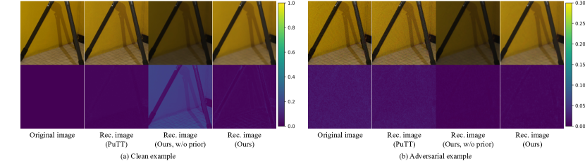
Figure 4: Visual comparison of the denoising task. Top: the original image and corresponding reconstructed image for (a) the clean example and (b) the adversarial example, using PuTT and our proposed method. Bottom: the error maps are created (a) between the rec. clean example and the original clean example, as well as (b) between the rec. adversarial example and the rec. clean example.

Table 7: Performance comparison of various methods on the denoising task. We evaluate the accuracy, NRMSE, SSIM and PSNR metrics using clean examples and adversarial examples on CIFAR-10. Additionally, we compare the differences between rec. AEs and rec. CEs.

Defense	CLN: CEs $\text{ }\&\text{ }$ rec. CEs				ADV: AEs $\text{ }\&\text{ }$ rec. AEs				REC: rec. CEs $\text{ }\&\text{ }$ rec. AEs
method	Acc.	NRMSE	SSIM	PSNR	Acc.	NRMSE	SSIM	PSNR	NRMSE	SSIM	PSNR
Standard	94.73	-	-	-	0.00	-	-	-	-	-	-
TT	87.30	0.0507	0.9526	31.14	36.13	0.065	0.8977	28.99	0.0267	0.9790	39.10
TR	94.34	0.0171	0.9938	40.58	0.98	0.0464	0.9210	31.91	0.0322	0.9598	35.51
QTT	84.57	0.0613	0.9253	29.49	51.56	0.0724	0.8808	28.06	0.0233	0.9855	39.88
QTR	83.40	0.0613	0.9254	29.49	49.41	0.0724	0.8785	28.06	0.0231	0.9853	39.96
PuTT	80.86	0.0626	0.9261	29.32	44.14	0.0742	0.8787	27.84	0.0311	0.9770	38.03
Ours	82.23	0.0644	0.9203	29.06	55.27	0.0748	0.8707	27.77	0.0218	0.9863	40.37

Results analysis on multiple attacks: Figure 3 shows the comparison of robust accuracy against PGD+EOT and AutoAttack with $l_{\infty}$ ($\epsilon=8/255$) threat on CIFAR-10 with WideResNet-28-10. When facing different attacks within the same threat, AT methods (Gowal et al., 2020, 2021; Pang et al., 2022) exhibit better generalization than AP methods (Yoon et al., 2021; Nie et al., 2022; Lee & Kim, 2023). Typically, robustness evaluation is based on the worst-case results of the robust accuracy. Under this criterion, our method outperforms all AT and AP methods. Furthermore, compared to the state-of-the-art AP method on both attacks, our method improves the average robust accuracy by 9.39%.

Results analysis on different datasets: Section 5.3 shows the generalization of the methods across different datasets. As previously mentioned, the existing AP methods typically rely on the specific datasets. When a pre-trained generative model trained on CIFAR-10 is applied to adversarial robustness evaluation on CIFAR-100, both standard accuracy and robust accuracy on CIFAR-100 drop significantly. This occurs because the pre-trained generative model can only generate the data it has learned. Although the input examples originate from CIFAR-100, the generative model attempts to output one of the ten classes from CIFAR-10, severely distorting the semantic information of the input examples and leading to low classification accuracy. In contrast, TN-based AP methods rely solely on the input examples rather than prior information learned from large datasets, allowing them generalize effectively across different datasets. The results demonstrate that our method exhibits strong generalization across different datasets, achieving comparable robust performance on CIFAR-100 as on CIFAR-10. Specifically, compared to the AP method (Nie et al., 2022), our method improves the average robust accuracy by 6.47%.

5.4 Denoising tasks

In this section, we evaluate the effectiveness of our method on non-classification tasks through visual comparisons and various quantitative metrics.

Visualization results analysis: Figure 4 shows the visual comparison of the denoising task on ImageNet. The top row in (a) displays the input clean example (CE), and its corresponding reconstructed clean examples (rec. CE) generated by PuTT and our proposed method, while (b) displays the reconstructed adversarial examples (rec. AE) for the input adversarial example (AE). Additionally, we create error maps to highlight differences, as shown at the bottom of Figure 4: (a) between the rec. CEs and the input CEs, and (b) between the rec. AEs and the rec. CEs. The results indicate that while our method does not match PuTT in reconstructing CEs, it significantly outperforms PuTT in removing adversarial perturbations from AEs.

Specifically, when processing CEs, the reconstructed examples generated by PuTT are almost identical to the original ones, whereas our method is slightly less effective in restoring some details. However, when processing AEs, the reconstructed examples from PuTT remain consistent with the original ones, leading to the preservation of adversarial perturbations, as highlighted in Figure 4b. In contrast, our method better removes those perturbations, ensuring that the rec. AEs and the rec. CEs retain similar information. Moreover, we evaluate the necessity of the second term in Eq. 1, which serves as a surrogate prior constraint to optimize the reconstructed examples toward the clean data distribution. As observed, removing this constraint eliminates prior information from the optimization process, increasing the likelihood of significant deviation in the wrong direction.

Quantitative results analysis: Table 7 shows the quantitative results of the denoising task for AEs and CEs of CIFAR-10. We compare our method with existing tensor network decomposition methods, including TT, TR, QTT, QTR, and PuTT. While our method does not achieve the best denoising performance on clean examples, it still maintains classification performance well, achieving 82.23% standard accuracy with the vanilla WideResNet-28-10 classifier. More importantly, our method outperforms others in the next two columns. Specifically, when processing AEs, our method yields the highest NRMSE and the lowest SSIM and PSNR, achieving the highest robust accuracy. This outcome is expected, as our goal is to ensure that the rec. AEs differ from the original AEs (i.e., lower SSIM and PSNR, and higher NRMSE in the “ADV” column) while rec. AEs closely resembling the rec. CEs (i.e., higher SSIM and PSNR, and lower NRMSE in the “REC” column). These results align well with the visual observations in Figure 4 and consistently demonstrate the effectiveness of our method highlighting its potential in adversarial scenarios.

Limitations  One limitation of our method is that, despite being a training-free technique, TN-based AP method requires additional optimization time during inference. This overhead stems from the inherent limitations of iterative optimization processes and impacts their practicality in real-world applications. Therefore, we leave the exploration of integrating our TN-based AP technique with more advanced and efficient optimization strategies for future research.

6 Conclusion

In this paper, we propose a novel model-free adversarial purification method based on a specially designed tensor network decomposition algorithm. We conduct extensive experiments on CIFAR-10, CIFAR-100, and ImageNet, demonstrating that our method achieves state-of-the-art performance in defending against adversarial attacks while exhibiting strong generalization across diverse adversarial scenarios. Despite these significant improvements, our method features an additional optimization cost during inference. However, further exploration of TN-based AP method remains an exciting research direction for developing a plug-and-play and effective adversarial purification technique.

Impact Statement

This paper presents work whose goal is to advance the field of Machine Learning. There are many potential societal consequences of our work, none which we feel must be specifically highlighted here.

Appendix

Appendix A Influence of different sampling methods

To support our hypothesis of using the average pooling, we test it with stride sampling, which selects pixels with constant strides. In principle, the stride sampling would not change the distribution of perturbations. Therefore, it serves as a baseline to compare the influence of distributions.

We test four types of noise distributions: (1) Gaussian $\mathcal{N}(0,0.3^{2})$, (2) Mixture of Gaussian (MoG), $0.5\cdot\mathcal{N}(-1.0,0.5^{2})+0.5\cdot\mathcal{N}(1.0,0.5^{2})$, (3) Beta distribution, $\text{Beta}(0.5,0.5)-0.5$, and (4) Uniform distribution, $\text{Uniform}(-0.5,0.5)$. For MoG, Beta and uniform noises, we scale them to have the same signal-to-noise ratio with the Gaussian distribution. We add the noises on the Girl image (Loeschcke et al., 2024) with resolution $1024\times 1024$. First, we show the noise distributions in Figure 5. As can be seen, the Avg Pooling strategy transforms the non-Gaussian noises into Gaussian-like noises, while the Stride sampling would not. Second, we run the PuTT algorithm with different sampling methods for 100 times. The violin plot of denoising results are shown in Figure 6. In Gaussian distribution, the Stride sampling is better than AvgPooling. While for non-Gaussian noises, the AvgPooling is more robust and better than Stride. The denoising results indicate that the average pooling can handle different types of noises, which is consistent with our hypothesis. However, as we introduced, this might not be enough, since we need to deal with the original image and noises in the final stage.

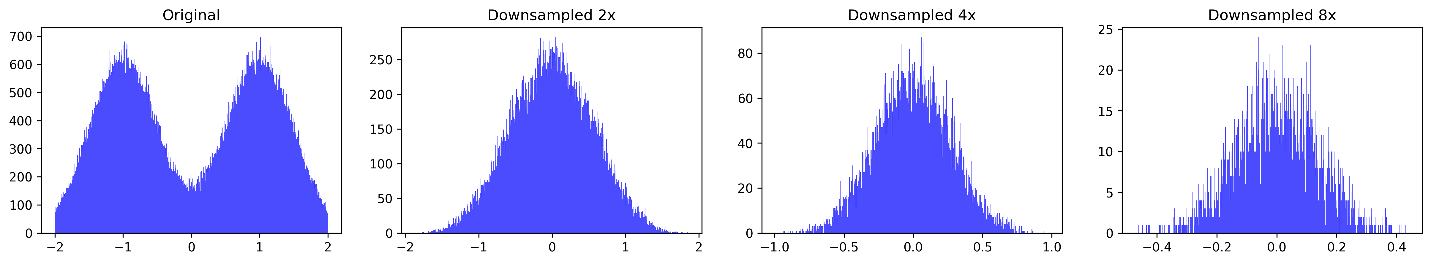
(a) MoG with Avg Pooling

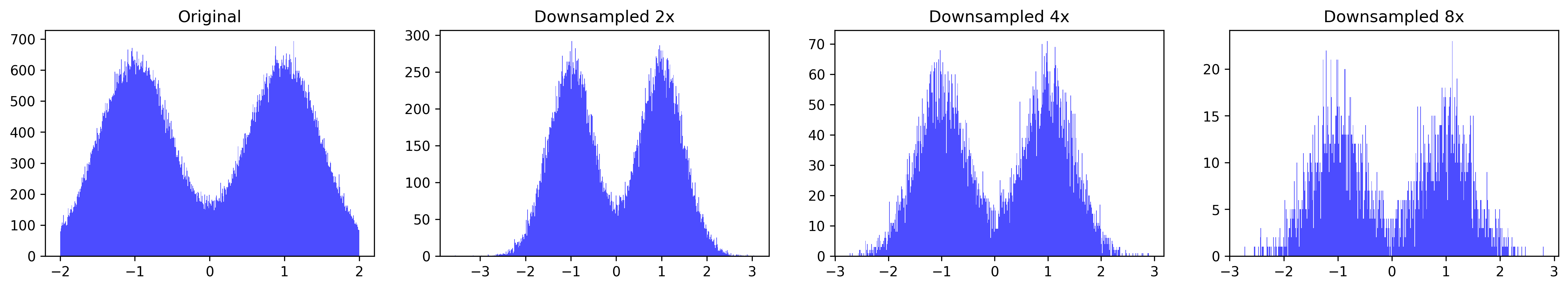
(b) MoG with Stride Sampling

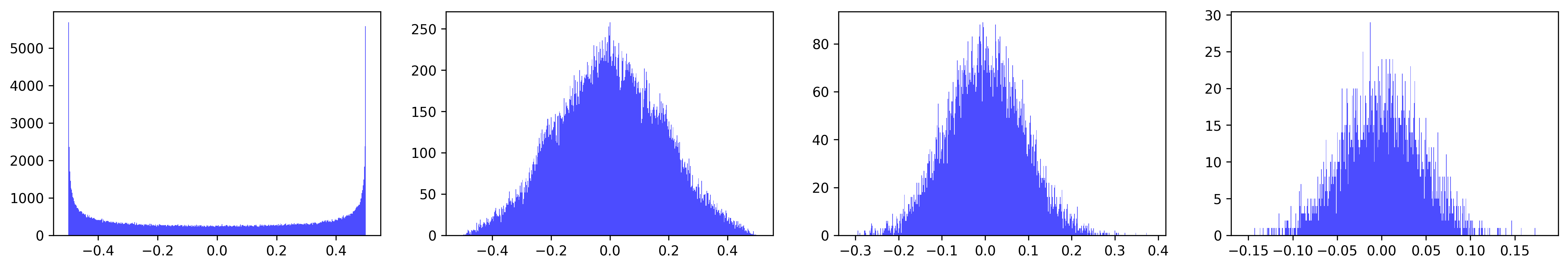
(c) Beta with Avg Pooling

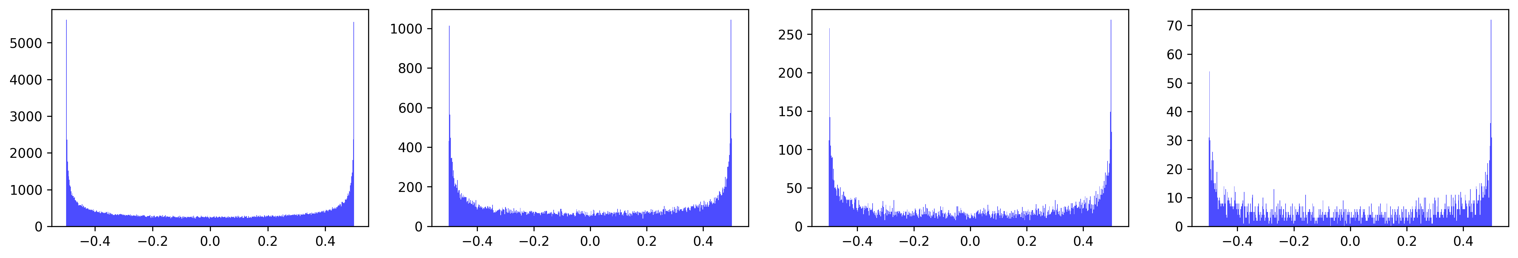
(d) Beta with Stride Sampling

(e) Uniform with Avg Pooling

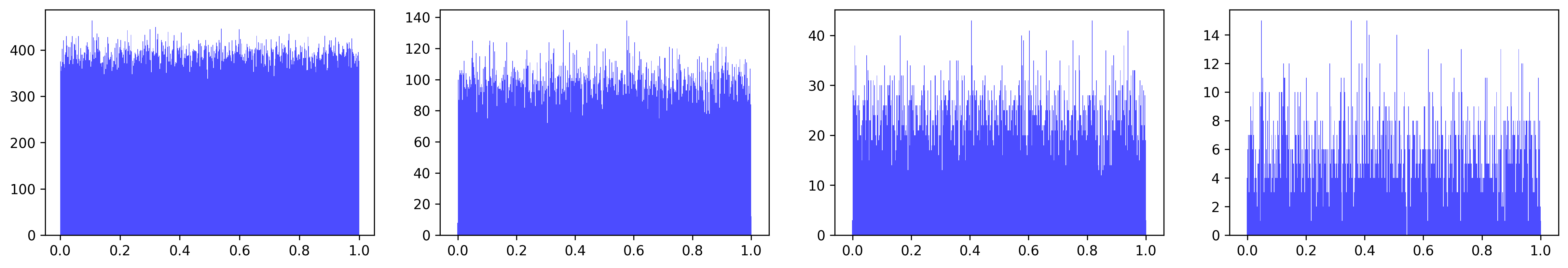
(f) Uniform with Stride Sampling

Figure 5: Histogram figures of noises under different sampling methods.

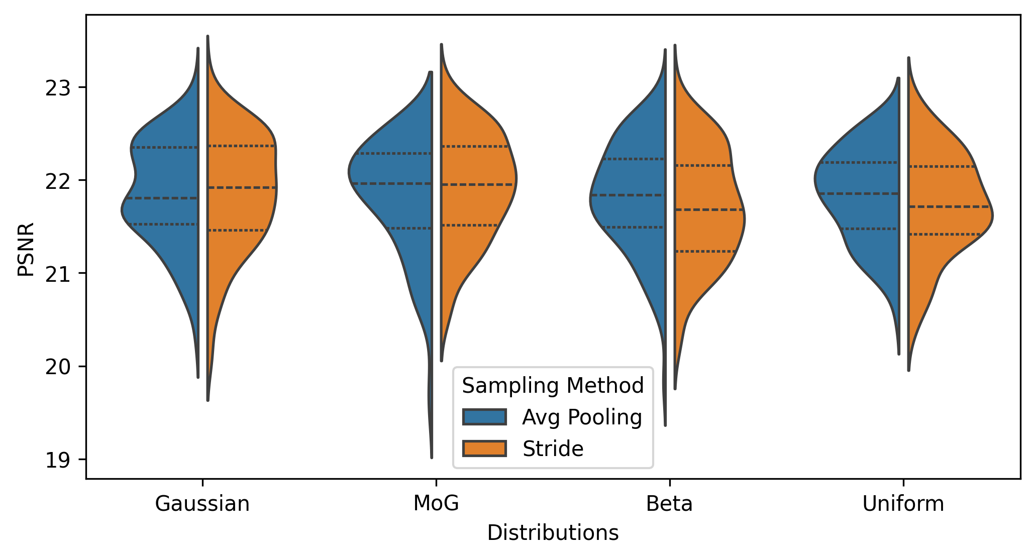
(a) PSNR

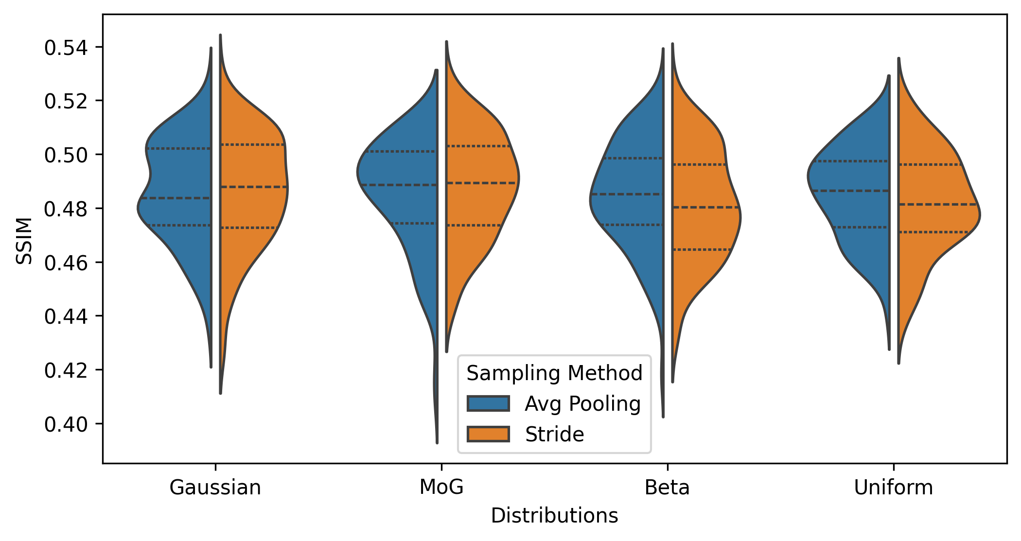
(b) SSIM

Figure 6: Violin plot of denoising results using different sampling methods. (a) PSNR results. (b) SSIM results.

Appendix B Tensor network decomposition

B.1 Matrix Product Operators

A matrix product operator (MPO) (McCulloch, 2008; Hubig et al., 2017) is the TN representation of a linear operator acting on a TT format, which makes it highly efficient to handle large operators. Namely, a linear operator $\boldsymbol{\mathcal{A}}:\mathbb{R}^{I_{1}\times\ldots\times I_{D}}\to\mathbb{R}^{J_{1}\times\ldots\times J_{D}}\,.$ Namely, if $\boldsymbol{\mathcal{Y}}=\boldsymbol{\mathcal{A}}\boldsymbol{\mathcal{X}}$, then each entry of $\boldsymbol{\mathcal{Y}}$ is given as

$${y}_{\mathbf{i}}=\sum_{i_{1}=1}^{I_{1}}\cdots\sum_{i_{D}=1}^{I_{D}}\boldsymbol{A}^{1}_{j_{1},i_{1}}\boldsymbol{A}^{2}_{j_{2},i_{2}}\ldots\boldsymbol{A}^{D}_{j_{D},i_{D}}\boldsymbol{X}^{1}_{i_{1}}\boldsymbol{X}^{2}_{i_{2}}\ldots\boldsymbol{X}^{D}_{i_{D}}\,,$$

B.2 Prolongation Operator

This work uses a specific MPO, known as the prolongation operator $\boldsymbol{\mathcal{P}}_{d}$ (Lubasch et al., 2018), to upsample a QTT format of an image from resolution $d-1$ to $d$.

Consider a one-dimensional vector $\boldsymbol{x}_{d}\in\mathbb{R}^{2^{d}}$. The matrix $\boldsymbol{P}_{2^{d}\to 2^{d+1}}$ upsamples $\boldsymbol{x}_{d}$ to $\boldsymbol{x}_{d+1}$ by linear interpolation between adjacent points. For example, for $d=2$,

$$\boldsymbol{P}_{4\to 8}=\begin{bmatrix}1&0&0&0\\ 0.5&0.5&0&0\\ 0&1&0&0\\ 0&0.5&0.5&0\\ 0&0&1&0\\ 0&0&0.5&0.5\\ 0&0&0&1\\ 0&0&0&0.5\end{bmatrix}$$

The matrix $\boldsymbol{P}_{2^{d}\to 2^{d+1}}$ can be written as an MPO $\boldsymbol{\mathcal{P}}_{d+1}$ entry-wise

$$p_{j_{1},\ldots,j_{d},i_{1},\ldots,i_{d+1}}=\boldsymbol{P}^{1}_{j_{1},i_{1}}\ldots\boldsymbol{P}^{d}_{j_{d},i_{d}}\boldsymbol{P}^{d+1}_{i_{d+1}}\,.$$

The entries are given explicitly (Lubasch et al., 2018) as

$$\boldsymbol{P}^{l}_{1,1}(1,1) =\boldsymbol{P}^{l}_{2,2}(1,1)=\boldsymbol{P}^{l}_{2,1}(1,2)=\boldsymbol{P}^{l}_{1,2}(2,2)=1,\forall l\in[d]$$

$$\boldsymbol{P}^{d+1}_{1}(1) =1\,,\boldsymbol{P}^{d+1}_{2}(1)=\boldsymbol{P}^{d+1}_{2}(2)=0.5\,,$$

and other entries are zero.

The prolongation operator described above applies to the QTT format of one-dimensional vectors. In general, this operator is the tensor product of the one-dimensional operators on each dimension: $\boldsymbol{\mathcal{P}}_{d}^{(2)}=\boldsymbol{\mathcal{P}}_{d}\otimes\boldsymbol{\mathcal{P}}_{d}$ for 2-dimensions (images) and $\boldsymbol{\mathcal{P}}_{d}^{(3)}=\boldsymbol{\mathcal{P}}_{d}\otimes\boldsymbol{\mathcal{P}}_{d}\otimes\boldsymbol{\mathcal{P}}_{d}$ for 3-dimensions (3D objects). For simplicity, since this work concerns only images, the superscript is omitted, denoting the prolongation operator as $\boldsymbol{\mathcal{P}}_{d}$.

Ultimately, for a resolution $d$ image $\boldsymbol{x}_{d}$, and $\boldsymbol{\mathcal{X}}_{d}=\operatorname{Q}(\boldsymbol{x}_{d})$, the upsampled image is resolution $d+1$, given as $\text{P}_{d}(\boldsymbol{x}_{d})=\operatorname{Q}^{-1}(\boldsymbol{\mathcal{P}}_{d}\boldsymbol{\mathcal{X}}_{d})$, where the linear function $\text{P}_{d}(\cdot)$ acts on the image level.

B.3 Recap of PuTT (Loeschcke et al., 2024)

A $2^{D}\times 2^{D}$ image, denoted as $\boldsymbol{x}_{D}$, can be quantized in to a $D$th order tensor $\boldsymbol{\mathcal{X}}_{D}=\text{Q}(\boldsymbol{x}_{D})$. Firstly, $\boldsymbol{x}_{D}$ is downsampled by average pooling to $\boldsymbol{x}_{D-l}$, correspondingly possesing a quantization $\boldsymbol{\mathcal{X}}_{D-l}$. Then, $D-l$ QTT cores of ${X}_{D-l}$ can be optimized by backpropagation, returning $\boldsymbol{\mathcal{Y}}_{D-l}$. The QTT cores of next resolution $\boldsymbol{\mathcal{X}}_{D-l+1}$ can be optimized similarly, initialized by the prologation $\boldsymbol{\mathcal{P}}_{D-l+1}(\boldsymbol{y}_{D-l})$. Repeat the process until the original resolution. (Loeschcke et al., 2024) demonstrates impressive reconstruction capability of PuTT thanks to the QTT structure and coarse-to-fine approach. The pseudocode is given in Algorithm 2.

Algorithm 2 PuTT (Loeschcke et al., 2024)

 Input: Image $\boldsymbol{x}_{D}$, number of iterations $T$, upsampling iterations $(t_{1},\ldots,t_{l})$.

 Output: TT reconstruction $\boldsymbol{y}_{D}=\text{PuTT}(\boldsymbol{x}_{D})$.

 $d\leftarrow D-l\,,\boldsymbol{x}_{d}\leftarrow\operatorname{AvgPool}(\boldsymbol{x}_{D})\,,\boldsymbol{\mathcal{X}}_{d}\leftarrow\operatorname{Q}(\boldsymbol{x}_{d})$

 for $t=1\to T$ do

  if $t\in(t_{1},\ldots,t_{l})$ then

   $d\leftarrow d+1$

   $\boldsymbol{x}_{d}\leftarrow\operatorname{AvgPool}(\boldsymbol{x}_{D})$

   $\boldsymbol{\mathcal{X}}_{d}\leftarrow\operatorname{Q}(\boldsymbol{x}_{d})$

  end if

  Loss $\ell\leftarrow\text{MSE}(\boldsymbol{\mathcal{Y}}_{d}-\boldsymbol{\mathcal{X}}_{d})$

  Update QTT cores $\boldsymbol{\mathcal{Y}}_{d}$ by backpropagation

 end for

 return $\boldsymbol{y}_{D}=\operatorname{Q}^{-1}(\boldsymbol{\mathcal{Y}}_{D})$

However, while PuTT aims to obtain better initialization by downsampling for better optimization and reconstruction, it does not account for adversarial examples or analyze the impact of downsampling on perturbations. Additionally, PuTT also minimizes the reconstruction loss on the input image, which inevitably results in the reconstruction of the perturbations. In contrast, we focus on the perturbations and propose a new optimization process introduced in the next section, aiming to reconstruct clean examples.

Appendix C More details of experimental settings

C.1 Implementation details of adversarial attacks

AutoAttack  We evaluate our method of defending against AutoAttack (Croce & Hein, 2020) and compare with the state-of-the-art methods as listed RobustBench benchmark (https://robustbench.github.io). For a comprehensive evaluation, we conduct experiments under all adversarial attack settings. Specifically, we set $\epsilon=8/255$ and $\epsilon=0.5/1.0$ for AutoAttack $l_{\inf}$ and AutoAttack $l_{2}$ threats on CIFAR-10. On CIFAR-100, we set $\epsilon=8/255$ for AutoAttack $l_{\inf}$. On ImageNet, we set $\epsilon=4/255$ for AutoAttack $l_{\inf}$.

PGD+EOT  We evaluate our method of defending against PGD+EOT (Madry et al., 2018; Athalye et al., 2018) and present the comparisons of AT methods, AP methods, and our method. Following the guidelines of Lee & Kim (2023), we set $\epsilon=8/255$ for PGD+EOT $l_{\inf}$ threats on CIFAR-10, where the update iterations of PGD is 200 with 20 EOT samples.

C.2 Implementation details of our method

For CIFAR-10, CIFAR-100 with resolution $32\times 32$ and ImageNet with resolution $224\times 224$, we first upsample them into resolution $2^{D}\times 2^{D}$ image $x_{D}$. Based on the initial experimental results, we set $D=8$, $l=1$, $\alpha=0.1$, $\eta=0.1$ and $N=1$ for the following experiments. The table results presented in the paper are conducted under these hyperparameters. This trick creates a large enough image to downsample until the perturbations are well mixed into Gaussian noise. Furthermore, without this initial step, the semantic information can become almost indistinguishable after several downsampling steps, especially for low-resolution images. For example, if a $32\times 32$ image is reduced with the factor of 8, the resolution $4\times 4$ image is of poor quality. Additionally, to more clearly observe the denoising effects in visualization results, we upsample the images to resolution $D=11$ with $\alpha=0.05$, $\eta=0.1$ and $N=3$ for the experiments in Figure 4, and comparisons in different downsampled images in Figure 1. The code will be available upon acceptance, with more details provided in the configuration files.

C.3 Implementation details of evaluation metrics

We evaluate the performance of defense methods using multiple metrics: Standard accuracy and robust accuracy (Szegedy et al., 2014) on classification tasks. For denoising tasks, we measure the Normalized Root Mean Squared Error (NRMSE, Botchkarev, 2018), Structural Similarity Index Measure (SSIM, Hore & Ziou, 2010), Peak Signal-to-Noise Ratio (PSNR) metrics between a reference image $\boldsymbol{x}$ and its reconstruction $\boldsymbol{y}$, where pixel values are in $[0,1]$. In denoising and reconstruction tasks, a lower NRMSE, a higher SSIM, and a higher PSNR generally indicate better performance.

Appendix D Inference time cost

Table 8: Inference time

Methods	CIFAR-10	CIFAR-100	ImageNet
AT	0.002 s	0.002 s	0.005 s
DM-based AP	1.49 s	1.50 s	5.11 s
Ours	12.39 s	11.81 s	14.10 s

Table 8 shows the inference time of different methods on CIFAR-10, CIFAR-100, and ImageNet, which is measured on a single image. Specifically, AP method purifies CIFAR data at a resolution of $32\times 32$ and ImageNet data at $256\times 256$, whereas our method operates at a resolution of $256\times 256$ across all datasets. As a form of Test-Time Training, our method inevitably increases inference cost. In a comparison at the same resolution of ImageNet, the AP method require 5.11 seconds, whereas our method takes 14.10 seconds. This overhead stems from the inherent limitations of iterative optimization processes and affects their practicality in real-world applications. We leave the study of integrating our TN-based AP technique with more advanced and faster optimization strategies for future research.

Appendix E Zero-shot adversarial defense

AT and AP methods depend heavily on external training dataset, overlooking the potential internal priors in the input itself. Among adversarial defense techniques, untrained neural networks such as deep image prior (DIP) (Ulyanov et al., 2018) and masked autoencoder (MAE) (He et al., 2022) have been utilized to avoid the need of extra training data (Dai et al., 2020, 2022; Lyu et al., 2023). However, although such deep learning models achieve high-quality reconstruction results, they have been shown to be susceptible to revive also the adversarial noise. This section compares two representative untrained models DIP and MAE.

Table 9: Comparison with untrained neural networks against AutoAttack $l_{\infty}$ threat ($\epsilon=8/255$) on CIFAR-10.

Defense method	Acc.	NRMSE	SSIM	PSNR
Clean examples
DIP	90.43	0.0464	0.9565	32.13
MAE	88.28	0.0847	0.8842	26.90
Ours	82.23	0.0644	0.9203	29.06
Adversarial examples
DIP	38.28	0.0451	0.9467	32.53
MAE	1.56	0.0914	0.8472	26.24
Ours	55.27	0.0748	0.8707	27.77

Table 9 shows that although DIP and MAE have achieved remarkable standard accuracy and reconstruction quality, they deteriorate significantly under attack.

Appendix F More discussion

As we all know, the adversarial challenge of attack and defense is endless. This contradiction arises from the fundamental difference between adversarial attacks and defenses. Attacks are inherently destructive, whereas defenses are protective. This adversarial relationship places the attacker in an active position, while the defender remains passive. As a result, attackers can continually explore new attack strategies against a fixed model to degrade its predictive performance, ultimately leading to the failure of conventional defenses. The introduction of TNP has the potential to address this issue. As a model-free technique, TNP generates tensor representations solely based on the input information. These representations dynamically change with each input, preventing attackers from exploiting a fixed model to generate effective adversarial examples. This defensive mechanism allows TNP to maintain a more proactive stance in the ongoing competition between adversarial attacks and defenses.

Appendix G Histogram and kernel density estimation results

Figure 7 shows the histogram and kernel density estimation of adversarial perturbations on 10 images. The distribution of those perturbations progressively aligns with that of Gaussian noise as the downsampling process progresses.

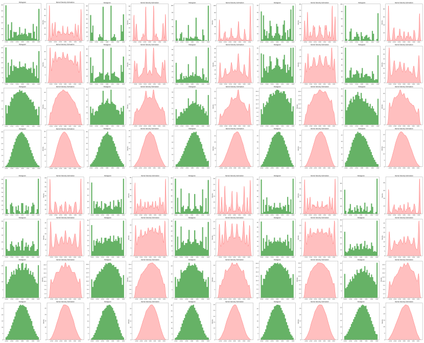
Figure 7: The histogram and kernel density estimation of adversarial perturbations in the downsampled images.

Appendix H Visualization

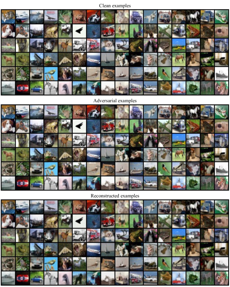
Figure 8: Clean examples (Top), adversarial examples (Middle) and reconstructed examples (Bottom) of CIFAR-10.

References

- Allen-Zhu & Li (2022) Allen-Zhu, Z. and Li, Y. Feature purification: How adversarial training performs robust deep learning. In 2021 IEEE 62nd Annual Symposium on Foundations of Computer Science (FOCS), pp. 977–988. IEEE, 2022.
- Athalye et al. (2018) Athalye, A., Engstrom, L., Ilyas, A., and Kwok, K. Synthesizing robust adversarial examples. In International conference on machine learning, pp. 284–293. PMLR, 2018.
- Augustin et al. (2020) Augustin, M., Meinke, A., and Hein, M. Adversarial robustness on in-and out-distribution improves explainability. In European Conference on Computer Vision, pp. 228–245. Springer, 2020.
- Bai et al. (2024) Bai, M., Huang, W., Li, T., Wang, A., Gao, J., Caiafa, C. F., and Zhao, Q. Diffusion models demand contrastive guidance for adversarial purification to advance. In Forty-first International Conference on Machine Learning, 2024.
- Bai et al. (2021) Bai, Y., Mei, J., Yuille, A. L., and Xie, C. Are transformers more robust than cnns? Advances in neural information processing systems, 34:26831–26843, 2021.
- Bai et al. (2023) Bai, Y., Anderson, B. G., Kim, A., and Sojoudi, S. Improving the accuracy-robustness trade-off of classifiers via adaptive smoothing. arXiv preprint arXiv:2301.12554, 2023.
- Bhattarai et al. (2023) Bhattarai, M., Kaymak, M. C., Barron, R., Nebgen, B., Rasmussen, K., and Alexandrov, B. S. Robust adversarial defense by tensor factorization. In 2023 International Conference on Machine Learning and Applications (ICMLA), pp. 308–315. IEEE, 2023.
- Botchkarev (2018) Botchkarev, A. Performance metrics (error measures) in machine learning regression, forecasting and prognostics: Properties and typology. arXiv preprint arXiv:1809.03006, 2018.
- Carmon et al. (2019) Carmon, Y., Raghunathan, A., Schmidt, L., Duchi, J. C., and Liang, P. S. Unlabeled data improves adversarial robustness. Advances in neural information processing systems, 32, 2019.
- Chen & Lee (2024) Chen, E.-C. and Lee, C.-R. Data filtering for efficient adversarial training. Pattern Recognition, 151:110394, 2024.
- Cichocki et al. (2015) Cichocki, A., Mandic, D., De Lathauwer, L., Zhou, G., Zhao, Q., Caiafa, C., and Phan, H. A. Tensor decompositions for signal processing applications: From two-way to multiway component analysis. IEEE signal processing magazine, 32(2):145–163, 2015.
- Croce & Hein (2020) Croce, F. and Hein, M. Reliable evaluation of adversarial robustness with an ensemble of diverse parameter-free attacks. In International conference on machine learning, pp. 2206–2216. PMLR, 2020.
- Croce et al. (2021) Croce, F., Andriushchenko, M., Sehwag, V., Debenedetti, E., Flammarion, N., Chiang, M., Mittal, P., and Hein, M. Robustbench: a standardized adversarial robustness benchmark. In Thirty-fifth Conference on Neural Information Processing Systems Datasets and Benchmarks Track (Round 2), 2021.
- Cui et al. (2024) Cui, J., Tian, Z., Zhong, Z., QI, X., Yu, B., and Zhang, H. Decoupled kullback-leibler divergence loss. In The Thirty-eighth Annual Conference on Neural Information Processing Systems, 2024.
- Dai et al. (2020) Dai, T., Feng, Y., Wu, D., Chen, B., Lu, J., Jiang, Y., and Xia, S.-T. Dipdefend: Deep image prior driven defense against adversarial examples. In Proceedings of the 28th ACM International Conference on Multimedia, MM ’20, pp. 1404–1412, New York, NY, USA, 2020. Association for Computing Machinery. ISBN 9781450379885. doi: 10.1145/3394171.3413898. URL https://doi.org/10.1145/3394171.3413898.
- Dai et al. (2022) Dai, T., Feng, Y., Chen, B., Lu, J., and Xia, S.-T. Deep image prior based defense against adversarial examples. Pattern Recognition, 122:108249, 2022.
- Debenedetti et al. (2023) Debenedetti, E., Sehwag, V., and Mittal, P. A light recipe to train robust vision transformers. In 2023 IEEE Conference on Secure and Trustworthy Machine Learning (SaTML), pp. 225–253. IEEE, 2023.
- Deng et al. (2009) Deng, J., Dong, W., Socher, R., Li, L.-J., Li, K., and Fei-Fei, L. Imagenet: A large-scale hierarchical image database. In 2009 IEEE conference on computer vision and pattern recognition, pp. 248–255. Ieee, 2009.
- Ding et al. (2019) Ding, G. W., Sharma, Y., Lui, K. Y. C., and Huang, R. Mma training: Direct input space margin maximization through adversarial training. In International Conference on Learning Representations, 2019.
- Dolatabadi et al. (2022) Dolatabadi, H. M., Erfani, S., and Leckie, C. l-inf robustness and beyond: Unleashing efficient adversarial training. In European Conference on Computer Vision, pp. 467–483. Springer, 2022.
- Engstrom et al. (2019) Engstrom, L., Ilyas, A., Salman, H., Santurkar, S., and Tsipras, D. Robustness (python library), 2019. URL https://github. com/MadryLab/robustness, 4(4):4–3, 2019.
- Entezari & Papalexakis (2022) Entezari, N. and Papalexakis, E. E. Tensorshield: Tensor-based defense against adversarial attacks on images. In MILCOM 2022-2022 IEEE Military Communications Conference (MILCOM), pp. 999–1004. IEEE, 2022.
- Goodfellow et al. (2015) Goodfellow, I. J., Shlens, J., and Szegedy, C. Explaining and harnessing adversarial examples. International Conference on Learning Representations, 2015.
- Gowal et al. (2020) Gowal, S., Qin, C., Uesato, J., Mann, T., and Kohli, P. Uncovering the limits of adversarial training against norm-bounded adversarial examples. arXiv preprint arXiv:2010.03593, 2020.
- Gowal et al. (2021) Gowal, S., Rebuffi, S.-A., Wiles, O., Stimberg, F., Calian, D. A., and Mann, T. A. Improving robustness using generated data. Advances in Neural Information Processing Systems, 34:4218–4233, 2021.
- Grzenda & Zieba (2008) Grzenda, W. and Zieba, W. Conditional central limit theorem. In Int. Math. Forum, volume 3, pp. 1521–1528, 2008.
- He et al. (2016) He, K., Zhang, X., Ren, S., and Sun, J. Deep residual learning for image recognition. In Proceedings of the IEEE conference on computer vision and pattern recognition, pp. 770–778, 2016.
- He et al. (2022) He, K., Chen, X., Xie, S., Li, Y., Dollár, P., and Girshick, R. Masked autoencoders are scalable vision learners. In Proceedings of the IEEE/CVF conference on computer vision and pattern recognition, pp. 16000–16009, 2022.
- Hendrycks et al. (2019) Hendrycks, D., Lee, K., and Mazeika, M. Using pre-training can improve model robustness and uncertainty. In International conference on machine learning, pp. 2712–2721. PMLR, 2019.
- Hore & Ziou (2010) Hore, A. and Ziou, D. Image quality metrics: Psnr vs. ssim. In 2010 20th international conference on pattern recognition, pp. 2366–2369. IEEE, 2010.
- Hubig et al. (2017) Hubig, C., McCulloch, I., and Schollwöck, U. Generic construction of efficient matrix product operators. Physical Review B, 95(3):035129, 2017.
- Ilyas et al. (2019) Ilyas, A., Santurkar, S., Tsipras, D., Engstrom, L., Tran, B., and Madry, A. Adversarial examples are not bugs, they are features. Advances in neural information processing systems, 32, 2019.
- Jia et al. (2022) Jia, X., Zhang, Y., Wu, B., Ma, K., Wang, J., and Cao, X. Las-at: adversarial training with learnable attack strategy. In Proceedings of the IEEE/CVF Conference on Computer Vision and Pattern Recognition, pp. 13398–13408, 2022.
- Khoromskij (2011) Khoromskij, B. N. O (d log n)-quantics approximation of n-d tensors in high-dimensional numerical modeling. Constructive Approximation, 34:257–280, 2011.
- Kolda & Bader (2009) Kolda, T. G. and Bader, B. W. Tensor decompositions and applications. SIAM review, 51(3):455–500, 2009.
- Krizhevsky et al. (2009) Krizhevsky, A., Hinton, G., et al. Learning multiple layers of features from tiny images. Technical Report, 2009.
- Laidlaw et al. (2021) Laidlaw, C., Singla, S., and Feizi, S. Perceptual adversarial robustness: Defense against unseen threat models. In International Conference on Learning Representations (ICLR), 2021.
- Lee & Kim (2023) Lee, M. and Kim, D. Robust evaluation of diffusion-based adversarial purification. In Proceedings of the IEEE/CVF International Conference on Computer Vision (ICCV), pp. 134–144, October 2023.
- Lin et al. (2024) Lin, G., Li, C., Zhang, J., Tanaka, T., and Zhao, Q. Adversarial training on purification (atop): Advancing both robustness and generalization. arXiv preprint arXiv:2401.16352, 2024.
- Loeschcke et al. (2024) Loeschcke, S. B., Wang, D., Leth-Espensen, C. M., Belongie, S., Kastoryano, M., and Benaim, S. Coarse-to-fine tensor trains for compact visual representations. In Forty-first International Conference on Machine Learning, 2024.
- Lubasch et al. (2018) Lubasch, M., Moinier, P., and Jaksch, D. Multigrid renormalization. Journal of Computational Physics, 372:587–602, 2018.
- Lyu et al. (2023) Lyu, W., Wu, M., Yin, Z., and Luo, B. Maedefense: An effective masked autoencoder defense against adversarial attacks. In 2023 Asia Pacific Signal and Information Processing Association Annual Summit and Conference (APSIPA ASC), pp. 1915–1922. IEEE, 2023.
- Madry et al. (2018) Madry, A., Makelov, A., Schmidt, L., Tsipras, D., and Vladu, A. Towards deep learning models resistant to adversarial attacks. In International Conference on Learning Representations, 2018.
- McCulloch (2008) McCulloch, I. P. Infinite size density matrix renormalization group, revisited. arXiv preprint arXiv:0804.2509, 2008.
- Nie et al. (2022) Nie, W., Guo, B., Huang, Y., Xiao, C., Vahdat, A., and Anandkumar, A. Diffusion models for adversarial purification. International Conference on Machine Learning, 2022.
- Oseledets (2011) Oseledets, I. V. Tensor-train decomposition. SIAM Journal on Scientific Computing, 33(5):2295–2317, 2011.
- Pang et al. (2022) Pang, T., Lin, M., Yang, X., Zhu, J., and Yan, S. Robustness and accuracy could be reconcilable by (proper) definition. In International Conference on Machine Learning, pp. 17258–17277. PMLR, 2022.
- Paszke et al. (2019) Paszke, A., Gross, S., Massa, F., Lerer, A., Bradbury, J., Chanan, G., Killeen, T., Lin, Z., Gimelshein, N., Antiga, L., et al. Pytorch: An imperative style, high-performance deep learning library. Advances in neural information processing systems, 32, 2019.
- Peng et al. (2023) Peng, S., Xu, W., Cornelius, C., Hull, M., Li, K., Duggal, R., Phute, M., Martin, J., and Chau, D. H. Robust principles: Architectural design principles for adversarially robust cnns. British Machine Vision Conference (BMVC), 2023.
- Phan et al. (2020) Phan, A.-H., Cichocki, A., Uschmajew, A., Tichavskỳ, P., Luta, G., and Mandic, D. P. Tensor networks for latent variable analysis: Novel algorithms for tensor train approximation. IEEE transactions on neural networks and learning systems, 31(11):4622–4636, 2020.
- Phan et al. (2023) Phan, H., Yin, M., Sui, Y., Yuan, B., and Zonouz, S. Cstar: towards compact and structured deep neural networks with adversarial robustness. In Proceedings of the AAAI Conference on Artificial Intelligence, volume 37, pp. 2065–2073, 2023.
- Rebuffi et al. (2021) Rebuffi, S.-A., Gowal, S., Calian, D. A., Stimberg, F., Wiles, O., and Mann, T. Fixing data augmentation to improve adversarial robustness. arXiv preprint arXiv:2103.01946, 2021.
- Rudkiewicz et al. (2024) Rudkiewicz, T., Ouerfelli, M., Finotello, R., Chaouai, Z., and Tamaazousti, M. Robustness of tensor decomposition-based neural network compression. In 2024 IEEE International Conference on Image Processing (ICIP), pp. 221–227. IEEE, 2024.
- Salman et al. (2020) Salman, H., Ilyas, A., Engstrom, L., Kapoor, A., and Madry, A. Do adversarially robust imagenet models transfer better? Advances in Neural Information Processing Systems, 33:3533–3545, 2020.
- Shi et al. (2021) Shi, C., Holtz, C., and Mishne, G. Online adversarial purification based on self-supervision. International Conference on Learning Representations, 2021.
- Song et al. (2024) Song, M., Choi, J., and Han, B. A training-free defense framework for robust learned image compression. arXiv preprint arXiv:2401.11902, 2024.
- Srinivasan et al. (2021) Srinivasan, V., Rohrer, C., Marban, A., Müller, K.-R., Samek, W., and Nakajima, S. Robustifying models against adversarial attacks by langevin dynamics. Neural Networks, 137:1–17, 2021.
- Szegedy et al. (2014) Szegedy, C., Zaremba, W., Sutskever, I., Bruna, J., Erhan, D., Goodfellow, I., and Fergus, R. Intriguing properties of neural networks. International Conference on Learning Representations, 2014.
- Ulyanov et al. (2018) Ulyanov, D., Vedaldi, A., and Lempitsky, V. Deep image prior. In Proceedings of the IEEE conference on computer vision and pattern recognition, pp. 9446–9454, 2018.
- Wang et al. (2022) Wang, J., Lyu, Z., Lin, D., Dai, B., and Fu, H. Guided diffusion model for adversarial purification. arXiv preprint arXiv:2205.14969, 2022.
- Wang et al. (2023) Wang, Z., Pang, T., Du, C., Lin, M., Liu, W., and Yan, S. Better diffusion models further improve adversarial training. International conference on machine learning, 2023.
- Wong et al. (2020) Wong, E., Rice, L., and Kolter, J. Z. Fast is better than free: Revisiting adversarial training. arXiv preprint arXiv:2001.03994, 2020.
- Yang et al. (2019) Yang, Y., Zhang, G., Katabi, D., and Xu, Z. Me-net: Towards effective adversarial robustness with matrix estimation. International Conference on Machine Learning, 2019.
- Yoon et al. (2021) Yoon, J., Hwang, S. J., and Lee, J. Adversarial purification with score-based generative models. In International Conference on Machine Learning, pp. 12062–12072. PMLR, 2021.
- Zagoruyko & Komodakis (2016) Zagoruyko, S. and Komodakis, N. Wide residual networks. In Procedings of the British Machine Vision Conference 2016. British Machine Vision Association, 2016.
- Zhang et al. (2020) Zhang, J., Zhu, J., Niu, G., Han, B., Sugiyama, M., and Kankanhalli, M. Geometry-aware instance-reweighted adversarial training. In International Conference on Learning Representations, 2020.
- Zhang et al. (2024) Zhang, M., Li, J., Chen, W., Guo, J., and Cheng, X. Classifier guidance enhances diffusion-based adversarial purification by preserving predictive information, 2024. URL https://openreview.net/forum?id=qvLPtx52ZR.
- Zhao et al. (2016) Zhao, Q., Zhou, G., Xie, S., Zhang, L., and Cichocki, A. Tensor ring decomposition. arXiv preprint arXiv:1606.05535, 2016.