A stochastic smoothing framework for nonconvex-nonconcave min-sum-max problems with applications to Wasserstein distributionally robust optimization

Abstract

Applications such as adversarially robust training and Wasserstein Distributionally Robust Optimization (WDRO) can be naturally formulated as min-sum-max optimization problems. While this formulation can be rewritten as an equivalent min-max problem, the summation of max terms introduces computational challenges, including increased complexity and memory demands, which must be addressed. These challenges are particularly evident in WDRO, where existing tractable algorithms often rely on restrictive assumptions on the objective function, limiting their applicability to state-of-the-art machine learning problems such as the training of deep neural networks. This study introduces a novel stochastic smoothing framework based on the log-sum-exp function, efficiently approximating the max operator in min-sum-max problems. By leveraging the Clarke regularity of the max operator, we develop an iterative smoothing algorithm that addresses these computational difficulties and guarantees almost surely convergence to a Clarke/directional stationary point. We further prove that the proposed algorithm finds an $\epsilon$-scaled Clarke stationary point of the original problem, with a worst-case iteration complexity of $\widetilde{O}(\epsilon^{-3})$. Our numerical experiments demonstrate that our approach outperforms or is competitive with state-of-the-art methods in solving the newsvendor problem, deep learning regression, and adversarially robust deep learning. The results highlight that our method yields more accurate and robust solutions in these challenging problem settings.

Keywords: stochastic method, smoothing method, nonconvex-nonconcave min-sum-max problem, minimax problems, distributionally robust optimization

Mathematics Subject Classification : 49M37, 65K05, 90C06, 90C30, 90C47

1 Introduction

The goal of this paper is to develop a novel algorithmic framework with guaranteed convergence for solving the nonconvex-nonconcave min-sum-max structured problem

$$\min_{{\mathbf{y}}\in\mathbb{R}^{m_{1}}}\left\{g({\mathbf{y}}):=\varphi({\mathbf{y}})+\mathbb{E}_{{\mathbf{x}}\sim\widehat{\mathbb{P}}_{n}}\left[\max_{{\mathbf{z}}\in\mathcal{Z}}\Psi({\mathbf{y}},{\mathbf{z}};{\mathbf{x}})\right]\right\}.$$ (P)

Here, ${\mathcal{Z}}\subseteq\mathbb{R}^{m_{2}}$ is a finite discrete set or a general continuous compact set. We refer to $g$ as the primal function with $\widehat{\mathbb{P}}_{n}$ as the uniform (empirical) distribution based on data set $\{{\mathbf{x}}_{1},{\mathbf{x}}_{2},\ldots,{\mathbf{x}}_{n}\}$. For each $i\in[n]$, we define

$$\Phi_{i}({\mathbf{y}}):=\max_{{\mathbf{z}}\in\mathcal{Z}}\Psi({\mathbf{y}},{\mathbf{z}};{\mathbf{x}}_{i}).$$ (1.1)

Throughout the paper, we make the following assumption on problem (P).

Assumption 1

The following statements hold:

$\mathrm{(i)}$ For each $i$, the function $\Psi(\cdot,\cdot;{\mathbf{x}}_{i}):\mathbb{R}^{m_{1}}\times\mathbb{R}^{m_{2}}\rightarrow\mathbb{R}$ is continuous on its domain, and its ${\mathbf{y}}$-partial gradient mapping $\nabla_{{\mathbf{y}}}\Psi(\cdot,\cdot;{\mathbf{x}}_{i})$ is also continuous.

$\mathrm{(ii)}$ The function $\varphi:\mathbb{R}^{m_{1}}\mapsto\mathbb{R}$ is proper closed convex, and its proximal mapping can be easily evaluated.

$\mathrm{(iii)}$ The sets ${\mathrm{dom}}(\varphi)$ and $\mathcal{Z}$ are compact.

Based on the above assumption, the functions $\{\Phi_{i}\}$ in (1.1) are well defined and continuous. The function $\varphi$ is any proximal-friendly convex function such as the indicator function of a convex set or the $L_{1}$-norm, often referred to as a regularizer. Notably, we do not assume smoothness of the functions $\{\Phi_{i}\}$ or $g$. The problem (P) encompasses a broad class of modern machine learning applications such as adversarially robust training goodfellow2014explaining ; huang2015learning ; madry2017towards ; liang2023optimization and distributionally robust optimization (DRO) kuhn2024distributionallyrobustoptimization ; rahimian2019distributionally . Notice that problem (P) can be equivalently written in the following minimax structured formulation

$$\min_{{\mathbf{y}}}\max_{\{{\mathbf{z}}_{1},\ldots,{\mathbf{z}}_{n}\}\subset\mathcal{Z}}\varphi({\mathbf{y}})+\frac{1}{n}\sum_{i=1}^{n}\Psi({\mathbf{y}},{\mathbf{z}}_{i};{\mathbf{x}}_{i}),$$ (1.2)

where we have used the fact that $\widehat{\mathbb{P}}_{n}$ is a uniform distribution. When solving problem (P), researchers liang2023implications often frame it as a minimax problem, as outlined in (1.2). However, directly solving (1.2) can result in computational difficulties, especially when $n$ is large in real-world applications, primarily due to the challenges in managing memory storage and tuning the step size during the optimization process.

To address this issue, some researchers deng2021local ; goodfellow2014explaining propose using a single ${\mathbf{z}}$ variable shared across all data points, and subsequently solve the corresponding problem

$$\min_{{\mathbf{y}}}\max_{{\mathbf{z}}\in\mathcal{Z}}\varphi({\mathbf{y}})+\frac{1}{n}\sum_{i=1}^{n}\Psi({\mathbf{y}},{\mathbf{z}};{\mathbf{x}}_{i}).$$ (1.3)

Nevertheless, this substitution fails to adequately capture the complexity of the original problem, resulting in solutions that deviate significantly from those of the original formulation.

Instead of maintaining $n$ ${\mathbf{z}}$-points in (1.2) or solving a deviated formulation in (1.3), we develop a framework to solve problem (P) by sequentially approximating the inner maximization problem using the Logarithm of the Expectation of Exponentials (log-sum-exp) approximation function shapiro2021lectures . By exploiting properties of this function, we directly solve the primal minimization problem $\min_{{\mathbf{y}}}g({\mathbf{y}})$ with a smoothing technique, effectively circumventing the computational challenges previously discussed. Our theoretical analysis shows that the proposed framework achieves a Clarke stationary point (see Definition 1), and importantly, we prove that this point is also a directional stationary point for the primal problem $\min_{{\mathbf{y}}}g({\mathbf{y}})$. The directional stationary point is shown to be the sharpest first-order stationary point of a nonconvex optimization problem pang2017computing ; cui2018composite ; cui2021modern . Notably, this is the first time that such a point is rigorously established for the nonconvex-nonconvave min-sum-max problem (P). The remainder of this section introduces relevant applications that have the structure of (P); we then state our technical contributions, a brief literature review, and finally list relevant notation and definitions.

1.1 Applications

Two relevant applications that have the structure of (P) are adversarially robust training and Wasserstein distributionally robust optimization (WDRO). In a classification setting, the adversarially robust training goodfellow2014explaining ; huang2015learning ; madry2017towards ; liang2023optimization problem takes the form of

$$\min_{{{\boldsymbol{\theta}}}}\frac{1}{n}\sum_{i=1}^{n}\max_{{\mathbf{z}}\in\Delta({{\mathbf{x}}}_{i})}\ell\left({\bar{{\mathbf{x}}}_{i}},f({\boldsymbol{\theta}},{\mathbf{z}})\right).$$ (1.4)

Here, $\{({\mathbf{x}}_{i},{\bar{{\mathbf{x}}}}_{i})\}_{i=1}^{n}\subset\mathbb{R}^{m_{2}}\times\mathbb{R}^{m_{3}}$ are sampled ordered pairs of data points and their corresponding labels (respectively), $\Delta({{\mathbf{x}}})=\left\{{\mathbf{z}}\in\mathbb{R}^{m_{2}}\big{|}d\left({{\mathbf{x}}},{\mathbf{z}}\right)\leq\varepsilon\right\}$ represents a set of feasible perturbations applied to a given data point ${\mathbf{x}}$ based on some distance function $d$, $f:\mathbb{R}^{m_{1}}\times\mathbb{R}^{m_{2}}\mapsto\mathbb{R}^{m_{3}}$ is a prediction function, and $\ell:\mathbb{R}^{m_{3}}\times\mathbb{R}^{m_{3}}\mapsto\mathbb{R}$ is a loss function. In the context of computer vision, this model seeks to identify the worst-case perturbations for images within a prescribed radius huang2015learning ; madry2017towards . Let $\widehat{\mathbb{P}}_{n}$ be a uniform distribution on the data samples. Then $\frac{1}{n}\sum_{i=1}^{n}\max_{{\mathbf{z}}\in\Delta({{\mathbf{x}}}_{i})}\ell\left({\bar{{\mathbf{x}}}_{i}},f({\boldsymbol{\theta}},{\mathbf{z}})\right)=\mathbb{E}_{({\mathbf{x}},\bar{\mathbf{x}})\in\widehat{\mathbb{P}}_{n}}\max_{{\mathbf{z}}\in\Delta({{\mathbf{x}}})}\ell\left({\bar{{\mathbf{x}}}},f({\boldsymbol{\theta}},{\mathbf{z}})\right)$, and thus (1.4) can be formulated into (P).

The WDRO problem kuhn2024distributionallyrobustoptimization can be formulated as

$$\min_{{\boldsymbol{\theta}}\in\Theta}\max_{\mathbb{P}\in\mathcal{B}_{\delta}(\widehat{\mathbb{P}}_{n})}\mathbb{E}_{{\mathbf{x}}\sim\mathbb{P}}\left[\ell({\boldsymbol{\theta}},{\mathbf{x}})\right],$$ (1.5)

where $\mathbb{P}$ is a probability distribution supported on ${\mathcal{Z}}$, $\ell:\mathbb{R}^{m_{1}}\times\mathbb{R}^{m_{2}}\mapsto\mathbb{R}$ is a given loss function, $\Theta$ is a closed convex set, $\mathbb{E}_{{\mathbf{x}}\sim\mathbb{P}}[\ell({\boldsymbol{\theta}},{\mathbf{x}})]=\int_{\mathcal{Z}}\ell({\boldsymbol{\theta}},{\mathbf{x}})\mathbb{P}(\mathrm{d}{\mathbf{x}})$, and the ambiguity set $\mathcal{B}_{\delta}(\widehat{\mathbb{P}}_{n})$ is defined as the $\delta$-ball in the $p$-th Wasserstein distance centered at the uniform distribution $\widehat{\mathbb{P}}_{n}$, i.e., $\mathcal{B}_{\delta}(\widehat{\mathbb{P}}_{n})=\{\mathbb{P}\in\mathcal{P}(\mathcal{Z})\mid d_{\mathcal{W}_{p}}(\mathbb{P},\widehat{\mathbb{P}}_{n})\leq\delta\}.$ Here, $\mathcal{P}(\mathcal{Z})$ is the space of probability distributions $\mathbb{P}$ supported on $\mathcal{Z}$ with $\mathbb{E}_{{\mathbf{x}}\sim\mathbb{P}}[\|{\mathbf{x}}\|]<\infty$, and the $p$-th Wasserstein distance kantorovich1958space between distributions $\mathbb{Q}_{1},\mathbb{Q}_{2}\in\mathcal{P}(\mathcal{Z})$ is defined by

$$d_{\mathcal{W}_{p}}\left(\mathbb{Q}_{1},\mathbb{Q}_{2}\right):=\inf\left\{\left(\int_{\mathcal{Z}\times\mathcal{Z}}\left\|{\mathbf{z}}_{1}-{\mathbf{z}}_{2}\right\|_{p}^{p}\mathrm{\Pi}\left(\mathrm{d}{\mathbf{z}}_{1},\mathrm{d}{\mathbf{z}}_{2}\right)\right)^{1/p}\bigg{|}\begin{array}[]{l}\mathrm{\Pi}\text{ is a joint distribution of }{\mathbf{z}}_{1}\text{ and }{\mathbf{z}}_{2}\text{ with}\\ \text{marginal distributions }\mathbb{Q}_{1}\text{ and }\mathbb{Q}_{2}\text{, respectively}\end{array}\right\}.$$

The inner maximization problem of WDRO gives the worst-case risk

$$\max_{\mathbb{P}\in\mathcal{B}_{\delta}(\widehat{\mathbb{P}}_{n})}\mathbb{E}_{{\mathbf{x}}\sim\mathbb{P}}\left[\ell({\boldsymbol{\theta}},{\mathbf{x}})\right].$$ (1.6)

Under certain assumptions on the loss function $\ell$, the optimal value of problem (1.6) is finite and attainable yue2022linear ; gao2023distributionally , and furthermore, strong duality holds. The dual problem of (1.6) is given by rahimian2019distributionally ; yue2022linear ; gao2023distributionally

$$\min_{\lambda\geq 0}\lambda\delta^{p}+\mathbb{E}_{{\mathbf{x}}\sim\widehat{\mathbb{P}}_{n}}\left[\max_{{\mathbf{z}}\in\mathcal{Z}}\{\ell({\boldsymbol{\theta}},{\mathbf{z}})-\lambda d({\mathbf{x}},{\mathbf{z}})\}\right]=\min_{\lambda\geq 0}\lambda\delta^{p}+\frac{1}{n}\sum_{i=1}^{n}\left[\max_{{\mathbf{z}}\in\mathcal{Z}}\{\ell({\boldsymbol{\theta}},{\mathbf{z}})-\lambda d({\mathbf{x}}_{i},{\mathbf{z}})\}\right].$$ (1.7)

Here, $d:\mathbb{R}^{m_{2}}\times\mathbb{R}^{m_{2}}\mapsto\mathbb{R}$ denotes the transport cost of the Wasserstein metric of order $p\in\mathbb{N}_{+}$ defined as $d({\mathbf{z}}_{1},{\mathbf{z}}_{2}):=\|{\mathbf{z}}_{1}-{\mathbf{z}}_{2}\|_{p}^{p}$ and $\lambda\in\mathbb{R}_{+}$ is the Lagrangian multiplier with respect to the inequality constraint $d_{\mathcal{W}_{p}}^{p}(\mathbb{P},\widehat{\mathbb{P}}_{n})\leq\delta^{p}$. By strongly duality, the optimal value of the aforementioned two models are the same. Therefore, by replacing (1.6) with (1.7) in problem (1.5), we arrive at the following problem

$$\min_{{\boldsymbol{\theta}}\in\Theta,\lambda\geq 0}g({\boldsymbol{\theta}},\lambda):=\lambda\delta^{p}+\mathbb{E}_{{\mathbf{x}}\sim\widehat{\mathbb{P}}_{n}}\left[\max_{{\mathbf{z}}\in\mathcal{Z}}\{\ell({\boldsymbol{\theta}},{\mathbf{z}})-\lambda d({\mathbf{x}},{\mathbf{z}})\}\right],$$ (1.8)

which is in the form of (P).

1.2 Literature Review

In this section, we briefly review existing methods for solving minimax problems and for WDRO. Also, we review the use of the log-sum-exp function.

1.2.1 Existing Methods for Solving Minimax Problems

Regardless of the dimension curse problem caused by a large $n$ in (1.2), existing algorithms for solving minimax problems can be applied there. Since the seminal work in v1928theorie , convex-concave minimax problems have been extensively studied based on the concept of saddle points (see e.g. chen2014optimal ; hamedani2021primal ; zhao2022accelerated ; daskalakis2018limit ; lan2023novel ; yan2022adaptive ; lin2020near and the references therein). Convex-nonconcave/nonconvex-concave minimax problems have also been studied; see zhang2024generalization ; xu2023unified ; lin2020gradient ; kong2021accelerated ; zhao2024primal ; rafique2022weakly ; lin2020near ; mancino2023variance ; zhang2022sapd+ ; zhang2024jointly ; xu2024decentralized and references therein. For nonconvex-nonconcave minimax structured problems, see Wang2020On ; li2022nonsmooth ; diakonikolas2021efficient ; grimmer2022landscape ; yang2022faster ; adolphs2019local ; daskalakis2018limit ; liu2021first ; fiez2021local ; mazumdar2019finding .

In cases where the minimax problem has a nonconvex-nonconcave structure, the existence of a saddle point is not guaranteed jiang2022optimality . Hence, researchers have turned to developing algorithms for finding the so-called game stationary point or Nash equilibrium point; see xu2023unified ; nouiehed2019solving ; jiang2022optimality ; liu2021first ; li2022nonsmooth for examples. However, for a game stationary point $(\bar{{\mathbf{y}}},[\bar{{\mathbf{z}}}_{i}]^{n}_{i=1})$, $\bar{{\mathbf{y}}}$ and $\bar{{\mathbf{z}}}_{i}$ may be far away from any local minimizer of problems $\min_{{\mathbf{y}}}g({\mathbf{y}})$ and $\min_{{\mathbf{z}}\in\mathcal{Z}}-\Psi(\bar{{\mathbf{y}}},{\mathbf{z}};{\mathbf{x}}_{i})$, respectively jiang2022optimality . Such a flaw occurs because a game stationary point fails to capture the order between the min-problem and the max-problem lin2020gradient .

To address the fundamental limitations of game stationary points, several works focus on minimizing the primal function $g$ to obtain stronger types of stationary points, such as the Clarke stationary point; see Definition 2 below. The Clarke stationarity has been studied for convex-concave and nonconvex-concave minimax problems lin2020gradient ; rahimian2019distributionally ; lu2020hybrid ; thekumparampil2019efficient . However, for nonconvex-nonconcave min-(sum-)max problems, computing (or even approximating) $\max_{{\mathbf{z}}}\Phi_{i}({\mathbf{y}},{\mathbf{z}};{\mathbf{x}})$ becomes intractable, making it difficult to verify the stationarity condition. In contrast, through the smoothing technique, our method can produce an iterate sequence converging to a Clarke stationary solution. Further, by establishing a Clarke regularity condition, we are able to show the convergence to a directional stationary point, which is claimed to be the sharpest first-order stationary point for nonconvex optimization problems pang2017computing ; cui2018composite ; cui2021modern .

1.2.2 Existing Methods for Solving WDRO

As introduced in rahimian2019distributionally , a broad approach in the DRO literature is to solve problem (1.8). Notably, problem (1.8) exhibits a min-sum-max structure, allowing methods for solving minimax problems to be applied to WDRO. As we have mentioned, the nonconcavity of the loss function presents significant challenges in obtaining a stationary point. Moreover, in WDRO, the function $\ell({\boldsymbol{\theta}},\cdot)-\lambda d({\mathbf{x}},\cdot)$ is often nonsmooth, further complicating the problem. To overcome these obstacles, researchers have proposed algorithms based on various reformulations of (1.8) (see e.g. in gao2023distributionally ; mohajerin2018data ; wozabal2012framework ; kuhn2019wasserstein ; liu2021discrete ), and the convergence of these methods requires somewhat stringent conditions on the loss function $\ell$ and the transport cost. When the support set $\cal{Z}$ is compact, a common approach to solve WDRO is to approximate $\cal{Z}$ using a finite, discrete grid. This method, though widely used xu2018distributionally ; chen2021decomposition ; liu2021discrete ; pflug2007ambiguity , becomes prohibitively expensive as the number of grid points grows. For WDRO with $l_{1}$ transport cost, a convex reformulation is available when the loss function can be expressed as a pointwise maximum of finitely many concave functions mohajerin2018data ; gao2023distributionally , or when the log-loss function is applied, such as in robust logistic regression li2019first ; selvi2022wasserstein ; shafieezadeh2015distributionally . Moreover, efficient first-order algorithms have been developed for specific WDRO problems where the function $\ell({\boldsymbol{\theta}},\cdot)-\lambda d(\cdot,{\mathbf{x}})$ is strongly concave blanchet2022optimal ; sinha2018certifiable . To guarantee the strong concavity, the transport cost must satisfy stringent conditions relative to the loss function. Without these conditions on the loss function or the transport cost, solving WDRO problems poses significant computational challenges. This is especially true when the structure of the problem does not lend itself to the simplifications used in previous work.

Recognizing the difficulty in solving the WDRO problem, wang2021sinkhorn innovatively proposes addressing a dual problem of Sinkhorn DRO (SDRO), which can be written as

$$\min_{{\boldsymbol{\theta}}\in\Theta,\lambda\geq 0}g_{\mathrm{s}}({\boldsymbol{\theta}},\lambda):=\lambda\delta^{p}+\lambda\eta\mathbb{E}_{{\mathbf{x}}\sim\widehat{\mathbb{P}}_{n}}\left[\log\mathbb{E}_{{\mathbf{z}}\sim\zeta}\left[e^{(\ell({\boldsymbol{\theta}},{\mathbf{z}})-\lambda d({\mathbf{x}},{\mathbf{z}}))/\lambda\eta}\right]\right]$$ (1.9)

for some $\eta>0$. The objective function in (1.9) can be viewed as a smoothing function of (1.8) by Definition 3 below with $\eta$ as the smoothing parameter. Assuming $\ell(\cdot,{\mathbf{z}})$ is convex for all feasible ${\mathbf{z}}$, the authors of wang2021sinkhorn develop a convergent triple-loop algorithm by skillfully combining a bisection method, a stochastic mirror descent method, and multilevel Monte-Carlo simulation. However, they fix $\eta>0$. In addition, in their complexity result (wang2021sinkhorn, , Theorem 3), they assume that any optimal solution $({\boldsymbol{\theta}}^{*},\lambda^{*})$ of problem (1.9) satisfies $\lambda^{*}\geq\overline{\lambda}$ for some positive scalar $\overline{\lambda}$. This assumption circumvents significant computational challenges by preventing both the Lipschitz constant and the gradient Lipschitz constant from exploding if $\lambda$ approaches 0 as the algorithm progresses, in which case, an exponential increase in the sampling complexity of their multilevel Monte-Carlo simulations would occur with respect to $\frac{1}{\lambda}$ (see the proof in (wang2021sinkhorn, , Proposition EC.4)). Hence, their algorithm does not solve the WDRO problem but rather addresses a simpler approximation.

In contrast, when applied to WDRO, our proposed method for (P) smoothes the function in (1.8) by the log-sum-exp technique and solves

$$\min_{{\boldsymbol{\theta}}\in\Theta,\lambda\geq 0}\widetilde{g}({\boldsymbol{\theta}},\lambda,\mu):=\lambda\delta^{p}+\mu\mathbb{E}_{{\mathbf{x}}\sim\widehat{\mathbb{P}}_{n}}\left[\log\mathbb{E}_{{\mathbf{z}}\sim\zeta}\left[e^{(\ell({\boldsymbol{\theta}},{\mathbf{z}})-\lambda d({\mathbf{x}},{\mathbf{z}}))/\mu}\right]\right].$$ (1.10)

Different from wang2021sinkhorn , we do not fix $\mu$ at a big number but instead push it to zero and we further treat $\lambda$ as a variable that can reach zero. The formulation in (1.10) replaces $\lambda\eta$ in (1.9) with $\mu$. However, this subtle difference in the formulation leads to a fundamentally different method from the algorithm in wang2021sinkhorn in terms of algorithmic development, methodological foundation, and theoretical analysis. First, wang2021sinkhorn solves a dual problem of SDRO with a fixed $\eta$. In contrast, we solve WDRO directly, requiring $\mu\downarrow 0$ in our algorithmic framework. This divergence alters the optimization objectives and methodological considerations. Second, the requirement of $\mu\downarrow 0$ introduces unique computational and theoretical challenges. It demands rigorous convergence analysis to prove that solving a sequence of smoothed problems approximates a WDRO solution, while also handling the ill-conditioning and increased computational complexity arising from the vanishing $\mu$. This necessitates sophisticated analysis and careful design to ensure stability and efficiency. Third, $\lambda$ is a primal variable in problem (1.9) and appears in the denominator of the exponential term. This results in both the Lipschitz constant and the gradient Lipschitz constant of $g_{s}$ with respect to $\lambda$ becoming unbounded as $\lambda$ approaches zero, which potentially yields slow convergence and high complexity. In constrast, the Lipschitz constant of $\widetilde{g}$ with respect to $\lambda$ is bounded, and the gradient Lipschitz constant of $\widetilde{g}$ with respect to $\lambda$ can be bounded by $\frac{C}{\mu}$ for some positive scalar $C$; this enables us to apply our established complexity results of our proposed method to the WDRO problem to obtain a scaled near-stationary solution; see Definition 4 below. Additionally, our proposed method applied to WDRO is a single-loop algorithm compared to the triple-loop algorithm developed in wang2021sinkhorn .

1.2.3 The Log-sum-exp Function

When $\mathcal{Z}$ is a finite discrete set, $\mu\log\frac{1}{|{\mathcal{Z}}|}\sum_{{\mathbf{z}}_{i}\in\mathcal{Z}}e^{\Phi({\mathbf{y}},{\mathbf{z}}_{i})/\mu}$ is the log-sum-exp function of $\max_{{\mathbf{z}}_{i}\in\mathcal{Z}}\Phi({\mathbf{y}},{\mathbf{z}}_{i})$. In the literature, this function is sometimes referred to as the softmax maximum lecun2015deep or the Neural Networks smoothing function chen2012smoothing ; burke2013gradient . This smoothing function has been used for solving finite minimax problems polak2003algorithms ; pee2011solving . It is useful in scenarios where a differentiable approximation for the maximum is required burke2020subdifferential ; boyd2004convex ; blanchet2020semi ; wang2023stochastic . Its optimization properties, such as convexity and gradient structure, have been studied extensively, highlighting its theoretical importance and practical utility in various fields ranging from statistics to deep learning. Notably, the gradient of the Neural Networks smoothing function can also be viewed as the softmax function lecun2015deep , which is widely used in neural networks. The authors in wang2023stochastic utilize the Neural Networks smoothing function to solve nonsmooth convex minimization problems. However, the log-sum-exp function that we will introduce in (2.2) has not yet been applied as an approximation of the max operator over a continuous compact set within any known smoothing algorithm.

1.3 Contributions

In this paper, we introduce the nonconvex-nonconcave min-sum-max problem (P), which encompasses applications such as adversarially robust training and Wasserstein distributionally robust optimization (WDRO). We design a first-order stochastic framework called SSPG (Stochastic Smoothing Proximal Gradient) to solve this problem effectively. Our key contributions are four-fold.

1. Under the assumptions that $\mathcal{Z}$ is compact and the Lipschitz continuity of $\Psi(\cdot,\cdot;{\mathbf{x}}_{i})$, we prove the Clarke regularity of $\Phi_{i}$ defined in (1.1) for each $i\in[n]$. By this property, we establish the equivalence between Clarke stationarity and directional stationarity for the primal problem in (P). This equivalence simplifies the algorithm design for the nonsmooth minimax problem and guarantees that once a Clarke stationary point is obtained, we attain a directional stationary point, which is known to represent the sharpest form of a first-order stationary point in nonsmooth nonconvex optimization problems pang2017computing ; cui2018composite ; cui2021modern . To the best of our knowledge, no prior work has identified a Clarke stationary point of a general nonconvex-nonconcave min-sum-max (or minimax) problem, even under Polyak-Łojasiewicz (PL) condition or Kurdyka-Łojasiewicz (KL) condition li2022nonsmooth ; nouiehed2019solving ; yang2020global ; yang2022faster .

2. We use the log-sum-exp function to approximate the inner maximization problem in nonconvex-nonconcave min-sum-max problems. By utilizing the properties of the log-sum-exp function, we show that when $\cal Z$ is a compact set, the resuling approximate function $\widetilde{\Phi}_{i}$ defined in (2.2) below is a smoothing function of $\Phi_{i}$ and it inherits the Lipschitz continuity of $\Psi(\cdot,\cdot;{\mathbf{x}}_{i})$ and $\nabla_{{\mathbf{y}}}\Psi(\cdot,{\mathbf{z}};{\mathbf{x}}_{i})$ for any ${\mathbf{z}}\in{\mathcal{Z}}$.

3. Using the smoothing technique, we develop SSPG as an iterative algorithmic framework for solving the nonconvex-nonconcave min-sum-max problem (P). The SSPG framework handles the sum part directly, thereby avoiding the potential memory burden associated with reformulating the original problem into (1.2). We prove that the proposed algorithm almost surely converges to a Clarke stationary point and a directionally stationary point of problem (P). We also prove that the proposed algorithm can, in expectation, find an $\epsilon$-scaled Clarke stationary point (see Definition 4 below) of the original problem, with a worst-case iteration complexity of $\widetilde{O}(\epsilon^{-3})$.

4. Our method can be directly applied to WDRO if a stochastic gradient estimator is available. We conduct extensive numerical experiments to assess the performance and effectiveness of our proposed method, yielding impressive results, particularly in terms of solution accuracy. Our evaluation encompasses three distinct problems within WDRO: newsvendor, regression, and adversarial robust deep learning. In each problem, our framework outperforms or is comparable to the state-of-the-art methods, demonstrating superior performance and robustness, highlighting the utility of our approach on real-world problems.

1.4 Definitions and Notations

Let $\|\cdot\|$ be the 2-norm of a vector. We use $[M]$ to represent $\{1,2,\ldots,M\}$ for an integer $M$. Given a compact set $\mathcal{Z}$, denote $|\mathcal{Z}|$ as the cardinality of $\cal{Z}$ if it is a finite set and volume of $\cal{Z}$ if it is a continuous set. The indicator function is denoted as $\mathbb{I}.$ The proximal mapping of a closed convex function $h$ is defined by $\operatorname{prox}_{h}({{\mathbf{x}}})=\operatorname*{arg\,min}_{\mathbf{z}}\{h({{\mathbf{z}}})+\frac{1}{2}\|{{\mathbf{z}}}-{{\mathbf{x}}}\|^{2}\}.$ We use $h^{\prime}\left(\bar{{\mathbf{y}}};{\mathbf{d}}\right)$ to denote the directional derivative of a function $h$ at $\bar{{\mathbf{y}}}$ along the direction ${\mathbf{d}}$, i.e.,

$$h^{\prime}\left(\bar{{\mathbf{y}}};{\mathbf{d}}\right)=\lim_{t\downarrow 0}\frac{1}{t}(h(\bar{{\mathbf{y}}}+t{\mathbf{d}})-h(\bar{{\mathbf{y}}})).$$ (1.11)

If the right limit in (1.11) exists, we say $h$ is directional differentiable at $\bar{{\mathbf{y}}}$ along the direction ${\mathbf{d}}$. It is known that if $h$ is piecewise differentiable and Lipschitz continuous, then it is directional differentiable mifflin .

Denote $h^{\circ}(\bar{{\mathbf{y}}};{\mathbf{d}})$ as the generalized directional derivative at $\bar{{\mathbf{y}}}$ along the direction ${\mathbf{d}}$ clarke1990optimization , by

$$h^{\circ}(\bar{{\mathbf{y}}};{\mathbf{d}}):=\limsup_{{{\mathbf{y}}\rightarrow\bar{{\mathbf{y}}}},{t\downarrow 0}}\frac{1}{t}(h({\mathbf{y}}+t{\mathbf{d}})-h({\mathbf{y}})).$$

In general, it holds $h^{\circ}(\bar{{\mathbf{y}}};{\mathbf{d}})\geq h^{\prime}\left(\bar{{\mathbf{y}}};{\mathbf{d}}\right)$ clarke1990optimization . If $h$ is differentiable, then $h^{\prime}\left(\bar{{\mathbf{y}}};{\mathbf{d}}\right)=h^{\circ}(\bar{{\mathbf{y}}};{\mathbf{d}})={\mathbf{d}}^{\top}\nabla h(\bar{{\mathbf{y}}})$. We use $\partial h$ to denote the (Clarke) subdifferential (clarke1990optimization, , Section 1.2) of a continuous function $h$, i.e.,

$$\partial h({\mathbf{y}}):=\left\{{\mathbf{z}}\in\mathbb{R}^{d}:\langle{\mathbf{z}},{\mathbf{v}}\rangle\leq h^{\circ}({\mathbf{y}};{\mathbf{v}}),\,\,\forall{\mathbf{v}}\in\mathbb{R}^{d}\right\}.$$

The normal cone of a convex set $\mathcal{Y}$ at ${\mathbf{y}}^{*}$ is defined as $\mathcal{N}_{\mathcal{Y}}({\mathbf{y}}^{*})=\{{\boldsymbol{\gamma}}:\langle{\boldsymbol{\gamma}},{\mathbf{y}}-{\mathbf{y}}^{*}\rangle\leq 0,\forall{\mathbf{y}}\in\mathcal{Y}\}.$

Definition 1 (Clarke regular (clarke1990optimization, , Definition 2.3.4))

A function $h$ is said to be Clarke regular at $\bar{{\mathbf{y}}}$ if for any direction ${\mathbf{d}}$, the directional derivative $h^{\prime}(\bar{{\mathbf{y}}};{\mathbf{d}})$ exists, and $h^{\prime}(\bar{{\mathbf{y}}};{\mathbf{d}})=h^{\circ}(\bar{{\mathbf{y}}};{\mathbf{d}})$.

From Definition 1, if $h$ is convex or differentiable, then it is Clarke regular clarke1990optimization and directional differentiable.

Definition 2 (Stationary point cui2021modern )

Let $h$ be a directional differentiable function. We say that ${\mathbf{y}}^{*}$ is a directional stationary point of problem $\min_{{\mathbf{y}}}h({\mathbf{y}})$ if $h^{\prime}({{\mathbf{y}}}^{*};{\mathbf{d}})\geq 0$ for all direction ${\mathbf{d}}$, and we say that ${\mathbf{y}}^{*}$ is a Clarke stationary point of problem $\min_{{\mathbf{y}}}h({\mathbf{y}})$ if $\mathbf{0}\in\partial h({\mathbf{y}}^{*})$.

Any directional stationary point of $h$ is also a Clarke stationary point, while it may not hold vice versa. Nevertheless, if $h$ is Clarke regular, then its Clarke stationary solution will also be a directional stationary point.

Definition 3 (Smoothing function chen2012smoothing )

Let $h:\mathbb{R}^{m}\mapsto\mathbb{R}$ be continuous. We call $\widetilde{h}:\mathbb{R}^{m}\times\mathbb{R}_{+}\mapsto\mathbb{R}$ a smoothing function of $h$, if for any fixed $\mu>0$, $\widetilde{h}(\cdot,\mu)$ is continuously differentiable, and for any $\bar{{\mathbf{y}}}$, it holds $\lim_{{\mathbf{y}}\rightarrow\bar{{\mathbf{y}}},\mu\downarrow 0}\widetilde{h}({\mathbf{y}},\mu)=h(\bar{{\mathbf{y}}})$.

1.5 Organization

The remainder of the paper is organized as follows. In Section 2, we introduce the SSPG framework for solving the problem (P). We first construct a smoothing function, then give our proposed algorithmic framework, and finally provide the convergence analysis. Numerical results are presented in Section 3. The proofs of some lemmas and theorems are given in Section 4. Finally, we conclude the paper in Section 5.

2 SSPG: A Stochastic Smoothing Proximal Gradient Framework for Solving Problem (P)

We focus on solving the primal problem $\min_{{\mathbf{y}}}g({\mathbf{y}})$ in (P). We first show that $g$ is Clarke regular under a Lipschitz condition in Section 2.1. Then we construct a smoothing function $\widetilde{\Phi}_{i}(\cdot,\mu)$ of $\Phi_{i}(\cdot)$ for each $i\in[n]$ in Section 2.2. With access to a stochastic gradient estimator, we introduce the SSPG method and establish its convergence results in Section 2.3.

2.1 Clarke Regularity of the Primal Function $g$

In this subsection, we prove that the primal function $g$ is directional differentiable and Clarke regular. We begin with a technical assumption.

Assumption 2 (Lipschitz)

There exists $l_{\Psi}>0$ such that $\|\nabla_{{\mathbf{y}}}\Psi({\mathbf{y}},{\mathbf{z}};{\mathbf{x}}_{i})\|\leq l_{\Psi}$ for all ${\mathbf{z}}\in\mathcal{Z}$ and ${\mathbf{y}}\in{\mathrm{dom}}(\varphi)$ and $\Psi({\mathbf{y}},\cdot;{\mathbf{x}}_{i})\text{ is }l_{\Psi}\text{-Lipschitz continuous on $\mathcal{Z}$}$ for all $i\in[n]$ and all ${\mathbf{y}}\in{\mathrm{dom}}(\varphi)$.

Before presenting the Clarke regularity result of $g$, we introduce two auxiliary lemmas.

Lemma 2.1 (mean-value theorem (correa1990subdifferential, , Proposition 1.1))

Let $h$ be a continuous directional differentiable function from $[a_{1},a_{2}]$ to $\mathbb{R}$. Then, there exists $\bar{a}\in(a_{1},a_{2})$ such that $h^{\prime}(\bar{a};1)\geq\frac{h(a_{1})-h(a_{2})}{a_{1}-a_{2}}.$

Lemma 2.2 ((correa1985directional, , Corollary 2.1))

Suppose Assumptions 1–2 hold. Then for each $i\in[n]$, the directional derivative $\Phi_{i}^{\prime}({\mathbf{y}};{\mathbf{d}})$ exists for all ${\mathbf{y}}$ and ${\mathbf{d}}$, and it satisfies

$$\Phi_{i}^{\prime}({\mathbf{y}};{\mathbf{d}})=\max\left\{{\mathbf{d}}^{\top}\nabla_{{\mathbf{y}}}\Psi({\mathbf{y}},\bar{{\mathbf{z}}};{\mathbf{x}}_{i})\mid\bar{{\mathbf{z}}}\in\operatorname*{arg\,max}_{{\mathbf{z}}\in\mathcal{Z}}\Psi({\mathbf{y}},{\mathbf{z}};{\mathbf{x}}_{i})\right\}.$$ (2.1)

Now, we are ready to show the key lemma of this subsection. The proof is given in Section 4.1.

Lemma 2.3 (Clarke regularity of the primal function)

Under Assumptions 1–2, the function $g$ in (P) is Clarke regular.

By Lemma 2.3, we have the following corollary.

Corollary 2.1

Under Assumptions 1–2, any Clarke stationary point of problem (P) is also a directional stationary point.

2.2 Constructing a Smoothing Function via the Log-sum-exp Function

For each $i\in[n]$, we construct a smoothing function for $\Phi_{i}$ by

$$\widetilde{\Phi}_{i}({\mathbf{y}},\mu)=\mu\log\mathbb{E}_{{\mathbf{z}}\sim\zeta}[e^{\Psi({\mathbf{y}},{\mathbf{z}};{\mathbf{x}}_{i})/\mu}],$$ (2.2)

where $\mu>0$ and the probability measure $\zeta$ satisfies the following assumption.

Assumption 3 (Measure)

$\mathrm{(i)}$ If $\mathcal{Z}$ is a finite discrete set, let $\zeta$ be a uniform distribution on $\cal{Z}$; $\mathrm{(ii)}$ If $\mathcal{Z}$ is a continuous compact set, we let ${\mathbf{z}}$ be a continuous random variable and $\mathrm{supp}(\zeta)$ be a compact subset in $\mathcal{Z}$ that contains at least one element in $\operatorname*{arg\,max}_{{\mathbf{z}}\in\mathcal{Z}}\Psi({\mathbf{y}},{\mathbf{z}};{\mathbf{x}}_{i})$.

We make the following assumption to ensure the smoothness of $\widetilde{\Phi}_{i}(\cdot,\mu)$.

Assumption 4 (Gradient Lipschitz)

There exists $L_{\Psi}>0$ such that $\nabla_{{\mathbf{y}}}{\Psi}(\cdot,{\mathbf{z}};{\mathbf{x}}_{i})$ is $L_{\Psi}$-Lipschitz continuous on ${\mathrm{dom}}(\varphi)$ for all ${\mathbf{z}}\in\mathcal{Z}$ and all $i\in[n]$.

The following lemma shows that $\widetilde{\Phi}_{i}$ is a smoothing function of $\Phi_{i}$ and establishes key properties of the smoothing function. Its proof is given in Section 4.2.

Lemma 2.4

Under Assumptions 1–4, the following statements hold:

1. $\widetilde{\Phi}_{i}$ is a smoothing function of $\Phi_{i}$ for each $i\in[n]$.

2. The ${\mathbf{y}}$ and $\mu$ partial gradients of $\widetilde{\Phi}_{i}$ are

   $$\nabla_{{\mathbf{y}}}\widetilde{\Phi}_{i}({\mathbf{y}},\mu)=\frac{\mathbb{E}_{{\mathbf{z}}\sim\zeta}[e^{\Psi({\mathbf{y}},{\mathbf{z}};{\mathbf{x}}_{i})/\mu}\nabla_{{\mathbf{y}}}\Psi({\mathbf{y}},{\mathbf{z}};{\mathbf{x}}_{i})]}{\mathbb{E}_{{\mathbf{z}}\sim\zeta}[e^{\Psi({\mathbf{y}},{\mathbf{z}};{\mathbf{x}}_{i})/\mu}]},$$

   $$\nabla_{\mu}\widetilde{\Phi}_{i}({\mathbf{y}},\mu)=\log\mathbb{E}_{{\mathbf{z}}\sim\zeta}[e^{\Psi({\mathbf{y}},{\mathbf{z}};{\mathbf{x}}_{i})/\mu}]-\frac{1}{\mu}\frac{\mathbb{E}_{{\mathbf{z}}\sim\zeta}[e^{\Psi({\mathbf{y}},{\mathbf{z}};{\mathbf{x}}_{i})/\mu}\Psi({\mathbf{y}},{\mathbf{z}};{\mathbf{x}}_{i})]}{\mathbb{E}_{{\mathbf{z}}\sim\zeta}[e^{\Psi({\mathbf{y}},{\mathbf{z}};{\mathbf{x}}_{i})/\mu}]}.$$

   Moreover, it holds that $\|\nabla_{{\mathbf{y}}}\widetilde{\Phi}_{i}({\mathbf{y}},\mu)\|\leq l_{\Psi}$ for any $\mu>0$, $\widetilde{\Phi}_{i}({\mathbf{y}},\mu_{1})\leq\widetilde{\Phi}_{i}({\mathbf{y}},\mu_{2})$ for any $\mu_{1}\geq\mu_{2}>0$, and $\lim_{\mu\downarrow 0}\mu\nabla_{\mu}\widetilde{\Phi}_{i}(\mathbf{y},\mu)=0$.

3. The ${\mathbf{y}}$ partial gradient $\nabla_{{\mathbf{y}}}\widetilde{\Phi}_{i}({\mathbf{y}},\mu)$ is $(L_{\Psi}+2l^{2}_{\Psi}/\mu)$-Lipschitz continuous with respect to ${\mathbf{y}}$ for any $\mu>0$.

For any $\mu_{1},\mu_{2}>0$ and all $i\in[n]$, we then establish upper bounds on the difference $|\widetilde{\Phi}_{i}({\mathbf{y}},\mu_{1})-\widetilde{\Phi_{i}}({\mathbf{y}},\mu_{2})|$ with respect to $|\mu_{1}-\mu_{2}|$ in the following two lemmas. Their proofs are given in Sections 4.3 and 4.4, respectively.

Lemma 2.5

Suppose Assumptions 1–4 hold, and $\mathcal{Z}$ is finite discrete. Then for any $\kappa\geq 2\log(|\cal Z|)$, ${\mathbf{y}}\in~{\mathrm{dom}}(\varphi)$, $1\geq\mu_{1}>\mu_{2}>0$, and all $i\in[n]$, it holds $|\widetilde{\Phi}_{i}({\mathbf{y}},\mu_{1})-\widetilde{\Phi}_{i}({\mathbf{y}},\mu_{2})|\leq\kappa(\mu_{1}-\mu_{2})$.

Lemma 2.6

Suppose Assumptions 1–4 hold,and $\mathcal{Z}$ is continuous compact. There exists $C_{0}\geq 2\log(|\cal{Z}|)$ such that $|\widetilde{\Phi}_{i}({\mathbf{y}},\mu_{1})-\widetilde{\Phi}_{i}({\mathbf{y}},\mu_{2})|\leq\frac{C_{0}}{\mu_{2}}(\mu_{1}-\mu_{2})$ for any ${\mathbf{y}}\in{\mathrm{dom}}(\varphi)$, $0<\mu_{1}\leq 1$, $\frac{1}{2}\mu_{1}\leq\mu_{2}\leq\mu_{1}$, and all $i\in[n]$.

Based on the smoothing function in (2.2), we introduce a “smoothing” problem of (P) as follows:

$$\min_{{\mathbf{y}}}\left\{\widetilde{g}({\mathbf{y}},\mu):=\varphi({\mathbf{y}})+\frac{1}{n}\sum_{i=1}^{n}\widetilde{\Phi}_{i}({\mathbf{y}},\mu)\right\}.$$ (2.3)

Definition 4 ($\epsilon$-scaled stationary point bian2013worst ; bian2015linearly )

We call ${\mathbf{y}}^{*}\in{\mathrm{dom}}(\varphi)$ an $\epsilon$-scaled stationary point of problem (P) in expectation, if it holds $\mathbb{E}[(\mathrm{dist}(0,\partial\widetilde{g}({\mathbf{y}}^{*},\mu)))^{2}]\leq\epsilon^{2}$, for some $0<\mu\leq\epsilon$.

Below we give our main theorem in this subsection. Its proof is given in Section 4.5.

Theorem 2.1 (Almost surely convergence to a directional stationary point)

Suppose Assumptions 1–4 hold. Let a sequence $\{\epsilon_{k}\}$ with $\sum_{k=0}^{\infty}\epsilon^{2}_{k}<+\infty$ , and $\{{\mathbf{y}}^{(k)}\}\subset{\mathrm{dom}}(\varphi)$ be given, such that ${\mathbf{y}}^{(k)}$ is an $\epsilon_{k}$-scaled stationary point of problem (P) in expectation. There exists $\{\mu_{k}\}$ such that $0<\mu_{k}\leq\epsilon_{k}$ for all $k\geq 0$, and

$$\lim_{k\rightarrow\infty}\mathrm{dist}(0,\partial\widetilde{g}({\mathbf{y}}^{{(k)}},\mu^{{(k)}}))=0,\text{ almost surely}.$$ (2.4)

Moreover, if there is a subsequence $\{{\mathbf{y}}^{(j_{k})}\}$ almost surely converging to ${\mathbf{y}}^{*}$, then ${\mathbf{y}}^{*}$ is a directioanlly stationary point of problem (P) almost surely.

Based on Theorem 2.1, we can pursue an $\epsilon$-scaled stationary point of problem (P) in expectation, in order to identify a directionally stationary point.

2.3 SSPG and Its Convergence Results

In this subsection, we present our proposed stochastic smoothing proximal gradient (SSPG) method for solving (P). When $n$ is large, accessing all $n$ samples at each iteration becomes computationally expensive. To overcome this challenge, at each iteration of SSPG, we choose $m$ samples $\{{\mathbf{x}}_{i_{1}},{\mathbf{x}}_{i_{2}},\ldots,{\mathbf{x}}_{i_{m}}\}$ uniformly at random without replacement from $\{{\mathbf{x}}_{1},{\mathbf{x}}_{2},\ldots,{\mathbf{x}}_{n}\}$. In addition, we assume the availability of stochastic gradient estimators $\{\mathcal{G}_{i}\}$ that satisfy

$$\mathbb{E}\left[\|\mathcal{G}_{i}({\mathbf{y}}^{(k)},\mu_{k})-\nabla_{{\mathbf{y}}}\widetilde{{\Phi}}_{i}({\mathbf{y}}^{(k)},\mu_{k})\|^{2}\right]\leq\widehat{\epsilon}_{k}^{2},\text{ for all }i\in[n],$$ (2.5)

for some scalar $\widehat{\epsilon}_{k}\geq 0$ and all $k\geq 0$. The $m$ sampled stochastic gradient estimates are then aggregated to form an overall estimator:

$$\mathcal{G}({\mathbf{y}}^{(k)},\mu_{k})=\frac{1}{m}\sum_{j=1}^{m}\mathcal{G}_{i_{j}}({\mathbf{y}}^{(k)},\mu_{k}).$$ (2.6)

We proceed with a proximal gradient update step, followed by updating the value of $\mu$ according to a predefined nonincreasing rule. The algorithmic framework is given in Algorithm 1.

Algorithm 1 A stochastic smoothing proximal gradient (SSPG) method for solving (P)

1:Initialization: choose ${\mathbf{y}}^{(0)}\in{\mathrm{dom}}(\varphi)$, $\mu_{0}>0$, a positive sequence $\{\widehat{\epsilon}_{k}\}_{\epsilon=0}^{K}$, and $K>0$.

2:for $k=0,1,\ldots,K$  do

3:   Let $\alpha_{k}>0$ be a stepsize, and $\mathcal{G}({\mathbf{y}}^{(k)},\mu_{k})$ is given in (2.6). Update ${\mathbf{y}}$ by

$${\mathbf{y}}^{(k+1)}=\operatorname{Prox}_{\alpha_{k}\varphi}\left({\mathbf{y}}^{(k)}-{\alpha_{k}}{}\mathcal{G}({\mathbf{y}}^{(k)},\mu_{k})\right).$$ (2.7)

4:   Choose $\mu_{k+1}\leq\mu_{k}$.

5:end for

Remark 2.1

We make a few remarks regarding the feasibility of establishing the condition in (2.5). First, if the set $\mathcal{Z}$ is finite, the exact value of $\nabla_{{\mathbf{y}}}\widetilde{\Phi}_{i}({\mathbf{y}}^{(k)},\mu_{k})$ can be calculated, ensuring $\widehat{\epsilon}_{k}=0$. This situation is common in Wasserstein distributionally robust optimization (WDRO) where a discrete grid is used to approximate the entire sample space xu2018distributionally ; chen2021decomposition ; liu2021discrete ; pflug2007ambiguity . Second, if for all $i\in[n]$, the expectation $\mathbb{E}_{{\mathbf{z}}\sim\zeta}e^{\Psi({\mathbf{y}},\cdot;{\mathbf{x}}_{i})/\mu}$ can be computed, we can generate samples to approximate the expectation $\mathbb{E}_{{\mathbf{z}}\sim\zeta}e^{\Psi({\mathbf{y}},\cdot;{\mathbf{x}}_{i})/\mu}\nabla_{{\mathbf{y}}}\Psi({\mathbf{y}},\cdot;{\mathbf{x}}_{i})$. By doing so, we can generate an unbiased stochastic gradient estimator of $\nabla_{{\mathbf{y}}}\widetilde{\Phi}_{i}({\mathbf{y}}^{(k)},\mu_{k})$. This approach is feasible in some specific cases, as detailed in Appendix A.1. Lastly, if we can obtain an approximate maximizer of problem $\max_{{\mathbf{z}}\in\mathcal{Z}}\Psi({\mathbf{y}},{\mathbf{z}};{\mathbf{x}}_{i})$ for all $i\in[n]$, we can efficiently construct such a stochastic gradient estimator, as detailed in Appendix A.2. Several conditions can ensure the computation of an approximate maximizer, such as (strong) concavity assumed in lin2020near ; thekumparampil2019efficient ; nouiehed2019solving ; kong2021accelerated , PL/KL conditions assumed in yang2020global ; yang2022faster ; li2022nonsmooth , and a subdifferential error bound condition. We emphasize that even under these conditions, our algorithm is new and our theoretical results are novel. We do not assume smoothness of $\Psi({\mathbf{y}},\cdot;{\mathbf{x}}_{i})$ which is required in lin2020near ; thekumparampil2019efficient ; nouiehed2019solving ; yang2020global ; yang2022faster ; li2022nonsmooth ; also, we guarantee convergence to a directional stationary point, a result that has not been achieved in existing works for solving nonconvex-nonconcave minimax problems.

The following lemma will be used for establishing the convergence results of Algorithm 1. Its proof is given in Section 4.6.

Lemma 2.7

Suppose Assumptions 1–4 hold. Let $\{{\mathbf{y}}^{(k)}\}$ and $\{\mu_{k}\}$ be the sequences generated by Algorithm 1 with $m=\min\{\lceil 4l_{\Psi}^{2}\widehat{\epsilon}_{k}^{-2}\rceil,n\}$ and $\alpha_{k}=\frac{\mu_{k}}{C_{2}}$ for all $k\in[K]$, where $C_{2}=L_{\Psi}\mu_{0}+2l^{2}_{\Psi}$. Then, for all $k\in[K-1]$,

1. the sequence $\left\{\widetilde{g}({\mathbf{y}}^{(k)},\mu_{k})\right\}$ satisfies

   $$\mathbb{E}\left[\widetilde{g}({\mathbf{y}}^{(k+1)},\mu_{k})-\widetilde{g}({\mathbf{y}}^{(k)},\mu_{k})\right]\leq-\frac{L^{(k)}}{4}\mathbb{E}\left[\|{\mathbf{y}}^{(k+1)}-{\mathbf{y}}^{(k)}\|^{2}\right]+\frac{4}{L^{(k)}}\widehat{\epsilon}_{k}^{2};$$ (2.8)

2. and it holds

   $$\mathbb{E}\left[\left(\mathrm{dist}\left(\mathbf{0},\partial\widetilde{g}({\mathbf{y}}^{(k+1)},\mu_{k})\right)\right)^{2}\right]\leq 18L^{(k)}\mathbb{E}\left[\widetilde{g}({\mathbf{y}}^{(k)},\mu_{k})-\widetilde{g}({\mathbf{y}}^{(k+1)},\mu_{k})\right]+{112}{}\widehat{\epsilon}_{k}^{2}.$$ (2.9)

Now we are ready to present the main convergence rate result. The proof is given in Section 4.7.

Theorem 2.2 (Stationarity violation bound)

Suppose Assumptions 1–4 hold. Let $0<\epsilon<1$, and $K>k_{1}\geq 0$ be given. Set $m=\min\{\lceil 4l_{\Psi}^{2}\widehat{\epsilon}_{k}^{-2}\rceil,n\}$, and $\alpha_{k}=\frac{\mu_{k}}{C_{2}}$ for all $k\in[K]$, where $C_{2}=L_{\Psi}\mu_{0}+2l^{2}_{\Psi}$. Let $\tau$ be randomly sampled from $\{k_{1},k_{1}+1,\ldots,K-1\}$ with probability $\operatorname{Prob}(\tau=k)=\frac{\mu_{k}}{\sum_{t=k_{1}}^{K-1}\mu_{t}}$. Then,

$$\mathbb{E}\left[\left(\mathrm{dist}\left(0,\partial\widetilde{g}({\mathbf{y}}^{(\tau+1)},\mu_{\tau})\right)\right)^{2}\right]$$

$$\leq \frac{18C_{2}\mathbb{E}\left[\widetilde{g}({\mathbf{y}}^{(k_{1})},\mu_{k_{1}})-\widetilde{g}({\mathbf{y}}^{(K)},\mu_{K-1})\right]}{\sum_{k=k_{1}}^{K-1}{\mu_{k}}}+\frac{18\sum_{k=k_{1}}^{K-2}\frac{C_{0}C_{2}}{\mu_{k+1}}\left(\mu_{k}-\mu_{k+1}\right)}{\sum_{k=k_{1}}^{K-1}{\mu_{k}}}+\frac{112\sum_{k=k_{1}}^{K-1}{\mu_{k}}{}\widehat{\epsilon}_{k}^{2}}{\sum_{k=k_{1}}^{K-1}{\mu_{k}}},$$ (2.10)

where $C_{0}$ is given in Lemma 2.6.

There are multiple strategies for selecting $\widehat{\epsilon}_{k}$ and $\mu_{k}$. Typically, we set $\widehat{\epsilon}_{k}$ in the same order as $\epsilon$. For $\mu_{k}$, it can be kept constant, decay over $k$, or be updated based on the difference between the objective function values at two consecutive iterations; see (3.4) in Section 3.1. As long as the right-hand side of (2.10) is less than $\epsilon^{2}$ and $\mu_{\tau}\leq\epsilon$, we claim that ${\mathbf{y}}^{\tau+1}$ is an $\epsilon$-scaled stationary point in expectation. Below, we present two corollaries detailing specific choices for $\widehat{\epsilon}_{k}$ and $\mu_{k}$, along with an analysis of the computational complexity required by Algorithm 1 to obtain an $\epsilon$-scaled stationary point. Their proofs are given in Section 4.8.

Corollary 2.2

Under the same assumptions of Theorem 2.2, set $k_{1}=0$, $\widehat{\epsilon}_{k}={\epsilon}/16$, and $\mu_{k}=\epsilon$ for all $k\in[K]$ with $K=\left\lceil 36C_{2}\epsilon^{-3}\widetilde{g}({\mathbf{y}}^{(0)},\epsilon)-\min_{{\mathbf{y}}}\widetilde{g}({\mathbf{y}},\epsilon)\right\rceil$. Then, Algorithm 1 outputs a point ${\mathbf{y}}^{(k)}$ satisfying $\mathbb{E}\left[\left(\mathrm{dist}\left(0,\partial\widetilde{g}({\mathbf{y}}^{(k+1)},\mu_{k})\right)\right)^{2}\right]\leq\epsilon^{2}$ with $\mu_{k}=\epsilon$ for some $0\leq k<K$. The total number of iterations required is $O(\epsilon^{-3})$.

Corollary 2.3

Under the same assumptions of Theorem 2.2, set $k_{1}=\lceil\epsilon^{-3}\rceil$, $\widehat{\epsilon}_{k}={\epsilon}/16$, and $\mu_{k}=(k+1)^{-1/3}$ for all $k\in[K].$ Starting from $k=k_{1}$, Algorithm 1 outputs ${\mathbf{y}}^{(k)}$ satisfying $\mathbb{E}\left[\left(\mathrm{dist}\left(0,\partial\widetilde{g}({\mathbf{y}}^{(k+1)},\mu_{k})\right)\right)^{2}\right]\leq\epsilon^{2}$ in no more than $O(\epsilon^{-3}\log(\epsilon^{-1}))$ iterations.

Remark 2.2

Let $\Delta=l_{\Psi}D$, where $D$ refers to the diameter of ${\mathrm{dom}}(\varphi)$. Since $\|\nabla_{{\mathbf{y}}}\widetilde{\Phi}_{i}({\mathbf{y}},\mu)\|\leq l_{\Psi}$ for all ${\mathbf{y}}\in{\mathrm{dom}}(\varphi)$ and $\mu>0$, we have $\widetilde{g}({\mathbf{y}}^{(k_{1})},\mu_{k_{1}})-\min_{{\mathbf{y}},\mu\in(0,1]}\widetilde{g}({\mathbf{y}},\mu)\leq\Delta$. By choosing $\widehat{\epsilon}_{k}=\mu_{k}/16$, we iteratively refine our approximations to the stationary point of problem (P). We construct a sequence $\{k_{t}\}$ via $k_{1}=0$, and $k_{t+1}=k_{t}+\lceil 36C_{2}t^{3}\Delta\rceil$ for all $t\geq 0$. We set $\mu_{k}=\frac{1}{t}$ for all $k_{t}\leq k<k_{t+1}$. According to Corollary 2.2, we obtain an $\epsilon_{t}=\frac{1}{t}$-scaled stationary point ${\mathbf{y}}^{(t)}$ in expectation between iterations $k_{t}$ and $k_{t+1}$. Since $\sum_{t=0}^{\infty}\epsilon^{2}_{t}=\sum_{t=0}^{\infty}\frac{1}{t^{2}}<+\infty$, Theorem 2.1 implies that any accumulation point of the sequence $\{{\mathbf{y}}^{(t)}\}$ is almost surely a directionally stationary point of problem (P).

3 Numerical Experiments

In this section, we demonstrate the utility and applicability of Algorithm 1 and compare it with two existing methods: SDRO wang2021sinkhorn and Gradient Descent with Maximization Oracle (GDMax) jin2020local . We explore three applications within the WDRO framework: the newsvendor problem, the regression problem, and the adversarial deep learning problem. All the numerical experiments are conducted using Python, with details provided in Table 1. We implement both SSPG and GDMax to solve problem (1.8), while for SDRO, we build on the code from GitHub to solve problem (1.9). The specific parameter values for each method are introduced separately in the following subsections for each application.

Problem Type	Processor Info
Newsvendor (Section 3.1) and regression problem (Section 3.2)	12th Gen Intel(R) Core(TM) i5-1240P with 8GB RAM
Adversarial robust deep learning problem (Section 3.3)	NVIDIA Ampere A100 GPU with 80 GB RAM

Table 1: Processor information

3.1 Newsvendor Problem

The newsvendor problem, which models the expected profit of a retailer under uncertain demand, takes the form of problem (1.5). In this subsection, we consider solving problems (1.8) and (1.9) with

$$\ell(\theta,x)=v\theta-u\min(\theta,x)\quad\text{and}\quad d(x,z)=\frac{1}{2}(x-z)^{2},$$ (3.1)

where $\theta\in\mathbb{R}_{+}$ represents the inventory level, $x\in\mathbb{R}$ denotes the demand, $v=5$ is the underage cost, and $u=7$ is the overage cost. To ensure that the inner maximization problem has a finite solution, we set $\lambda\geq 7$, as required in lee2021data .

Problem parameters: We synthetically generate five different demand datasets, each consisting of $n=100$ independent samples drawn from an exponential distribution with rate parameter 1. We set $\delta=1$ and $p=2$. For each dataset $X_{\mathrm{train}}$, the empirical distribution $\widehat{\mathbb{P}}_{n}$ is constructed from these $n$ samples for each dataset; the support set is given as $\mathcal{Z}=\{x:\min(X_{\mathrm{train}})\leq x\leq\max(X_{\mathrm{train}})\}$.

Algorithm parameters: For all the methods, we use the initial $\theta^{(0)}\sim\mathcal{U}(0,1)$ on all five datasets, where ${\mathcal{U}}$ denotes the uniform distribution. In addition, for GDMax and SSPG, we use the same $\lambda^{(0)}\sim\mathcal{U}(7,15)$ on all five datasets. For SSPG, we set $\mu_{0}=\lambda^{(0)}\eta$, where $\eta\sim\mathcal{U}(0.1,1)$. Following wang2021sinkhorn , we use a grid search for SDRO to fine-tune the hyperparameters $\lambda$ and $\eta$ from the sets {7, 10, 15} and {0.1, 0.5, 1}, respectively. Each method is terminated after 1000 iterations.

Implementation of the compared methods at the $k$th iteration: For each method, at iteration $k$, we solve several inner maximization problems to obtain $\{z_{i}^{(k+1)}\}_{i=1}^{n}\subset\mathbb{R}$. Specifically, for each $i\in\{1,2,\ldots,n\}$, we solve problem $\max_{z\in{\mathcal{Z}}}\ell(\theta^{(k)},z)-\lambda^{(k)}d(x_{i},z)$ using the projected gradient ascent with a fixed step size of $10^{-2}$ for 20 iterations, starting from $\mathrm{Proj}_{{\mathcal{Z}}}(x_{i}+10^{-3}s)$ where $s$ follows a standard normal distribution. After obtaining $\{z_{i}^{(k+1)}\}_{i=1}^{n}$, GDMax performs a projected gradient descent step on the primal variable $(\theta,\lambda)$ using the gradient $\nabla_{(\theta,\lambda)}\frac{1}{n}\sum_{i=1}^{n}\left[\lambda^{(k)}\delta^{p}+\ell({\boldsymbol{\theta}}^{(k)},z_{i}^{(k+1)})-\lambda^{(k)}d(x_{i},z_{i}^{(k+1)})\right]$ and a fixed learning rate of $0.1$.

For SSPG and SDRO, for all $i\in\{1,2,\ldots,n\}$, we generate sets $\Omega_{i}^{k}$ of size $M=32$, containing samples near $z_{i}^{(k+1)}$. For any $\widehat{z}\in\Omega_{i}^{k}$, we set $\widehat{z}=\mathrm{Proj}_{{\mathcal{Z}}}(z_{i}^{(k+1)}+s^{(k+1)})$ with $s^{(k+1)}\sim\mathcal{N}(0,10^{-1})$. SDRO then performs a projected gradient descent step on $\theta$ with gradient $\nabla_{\theta}{g}_{s}^{k}(\theta^{(k)},\lambda)$ and a fixed learning rate of $0.1$, where

$${g}_{s}^{k}(\theta,\lambda)=\lambda\delta^{p}+\lambda\eta\frac{1}{n}\sum_{i=1}^{n}\left[\text{log}\left(\frac{1}{M}\sum_{\widehat{z}\in\Omega_{i}^{k}}\left[e^{\frac{\ell(\theta,\widehat{z})-\lambda d(x_{i},\widehat{z})}{\lambda\eta}}\right]\right)\right].$$ (3.2)

Our SSPG method similarly conduct a projected gradient descent step on $(\theta,\lambda)$ with $\nabla_{(\theta,\lambda)}\widetilde{g}^{k}(\theta^{(k)},\lambda^{(k)},\mu_{k})$ and a fixed learning rate of $0.1$, where

$$\widetilde{g}^{k}(\theta,\lambda,\mu)=\lambda\delta^{p}+\mu\frac{1}{n}\sum_{i=1}^{n}\left[\text{log}\left(\frac{1}{M}\sum_{\widehat{z}\in\Omega_{i}^{k}}\left[e^{\frac{\ell(\theta,\widehat{z})-\lambda d(x_{i},\widehat{z})}{\mu}}\right]\right)\right].$$ (3.3)

We then update $\mu$ by

$$\mu_{k+1}=\left\{\begin{aligned} &\mu_{k},\hskip 76.82234pt\text{ if }\widetilde{g}^{k}(\theta^{(k+1)},\lambda^{(k+1)},\mu_{k})-\widetilde{g}_{k}(\theta^{(k)},\lambda^{(k)},\mu_{k})<-\mu_{k}^{2\sigma_{2}},\\ &\max\{\sigma_{1}\mu_{k},10^{-4}\mu_{0}\},\,\,\,\text{otherwise},\end{aligned}\right.$$ (3.4)

with $\sigma_{1}=0.99$, $\sigma_{2}=0.5$.

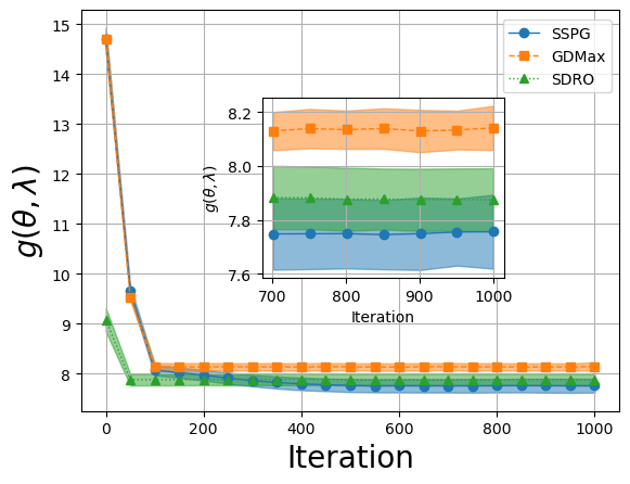
(a) $g(\theta,\lambda)$

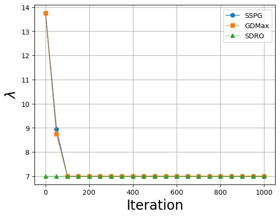
(b) $\lambda$ iterates

Figure 1: Comparison of $g(\theta,\lambda)$ and $\lambda$ among SSPG, GDMax, and SDRO for solving the newsvendor problem.

Performance comparisons: Figure 1(a) presents the mean and standard deviation of $g(\theta,\lambda)$ over iterations for SSPG, GDMax, and SDRO across the five training sets. This figure demonstrates that SSPG achieves lower values of $g(\theta,\lambda)$ compared to GDMax and SDRO, illustrating the advantage of employing a smoothing technique and dynamically updating $\lambda$ and $\mu$ for solving the newsvendor problem. Figure 1(b) shows the mean and standard deviation of $\lambda$. It reveals that SSPG and GDMax quickly converge to values of 7, while SDRO maintains a fixed $\lambda=7$. This choice arises from a grid search indicating that the pair $\lambda=7,\eta=0.1$ yields the best performance among the tested configurations for SDRO.

3.2 Regression Problem

The distributionally robust regression problem aims to find a robust solution to the standard regression problem by minimizing the worst-case risk. In this subsection, we consider problems (1.8) and (1.9) with

$$\ell({\boldsymbol{\theta}},{\mathbf{x}})=(h_{{\boldsymbol{\theta}}}({\mathbf{a}})-b)^{2},\text{ and }d({\mathbf{x}},{\mathbf{z}})=d(({\mathbf{a}},b),(\overline{{\mathbf{a}}},\overline{b}))=\frac{1}{2}\|{\mathbf{a}}-\overline{{\mathbf{a}}}\|_{2}^{2}+\infty|b-\overline{b}|,$$ (3.5)

where $h_{{\boldsymbol{\theta}}}:\mathbb{R}^{m_{2}-1}\to\mathbb{R}$ is a small neural network parameterized by ${\boldsymbol{\theta}}$, ${\mathbf{x}}=({\mathbf{a}},b)$, ${\mathbf{z}}=(\overline{{\mathbf{a}}},\overline{b})$ with ${\mathbf{a}},\overline{{\mathbf{a}}}\in\mathbb{R}^{m_{2}-1}$ representing a vector of features and $b,\overline{b}\in\mathbb{R}$ denoting a target. Specifically, we employ a neural network with a single hidden layer containing three neurons, using the ReLU activation function goodfellow2016deep . The $\infty$ before $|b-b{{}^{\prime}}|$ means that there is no uncertainty in the target variable.

Problem parameters: We set $\delta=10$ and $p=2$. For each dataset $X_{\mathrm{train}}$, the empirical distribution $\widehat{\mathbb{P}}_{n}$ is constructed from these $n$ samples for each dataset; the support set is given as $\mathcal{Z}=\widetilde{\mathcal{Z}}\times\mathbb{R}$ with $\widetilde{\mathcal{Z}}~=~\prod_{j=1}^{m_{2}-1}[\min([X_{\text{train}}]_{\cdot,j}),\max([X_{\text{train}}]_{\cdot,j})]$.

Datasets: We consider three real-world datasets, Space GA, BodyFat, and MG, from the LIBSVM repository. Each dataset, containing $n$ data points, is randomly partitioned into training (80%) and testing (20%) sets using train_test_split from Scikit-learn, ensuring that the original data distribution is preserved. The resulting training sets and test sets are $X_{\text{train}}\in\mathbb{R}^{\lfloor 0.8\times n\rfloor\times(m_{2}-1)}$ and $X_{\text{test}}\in\mathbb{R}^{\lceil 0.2\times n\rceil\times(m_{2}-1)}$, respectively. The testing set is further normalized using StandardScaler. To ensure fair comparisons, we employ five distinct random seeds for data preparation, including splitting, scaling, and initialization, ensuring identical dataset configurations across all three methods.

Algorithm parameters: For all the methods, we initialize $\theta^{(0)}$ by the default setting of pytorch. In addition, for GDMax and SSPG, we let $\lambda^{(0)}\sim\mathcal{U}(1,10)$. For SSPG, we set $\mu_{0}=\lambda^{(0)}\eta$, where $\eta\sim\mathcal{U}(0.1,1)$. Following wang2021sinkhorn , we utilize a grid search for SDRO to fine-tune the hyperparameters $\lambda$ and $\eta$ from the sets {1, 5,10} and {0.1, 0.5, 1}, respectively. For each comparison method, the training is terminated after 500 epochs.

Implementation of the compared methods at the $k$th iteration: For each method, at iteration $k$, we conduct an inner maximization step to obtain $\{{\mathbf{z}}_{i}^{(k+1)}=(\overline{{\mathbf{a}}}_{i}^{(k+1)},\overline{b}_{i}^{(k+1)})\}_{i=1}^{\lfloor 0.8\times n\rfloor}\subset\mathbb{R}^{m_{2}}$. Specifically, for each $i\in\{1,2,\ldots,\lfloor 0.8\times n\rfloor\}$, we solve problem $\max_{{\mathbf{z}}\in{\mathcal{Z}}}\ell({\boldsymbol{\theta}}^{(k)},{\mathbf{z}})-\lambda^{(k)}d({\mathbf{x}}_{i},{\mathbf{z}})$ using the projected gradient ascent with a fixed step size of $10^{-2}$ for five iterations, starting from ${\mathbf{x}}_{i}+10^{-3}{\mathbf{s}}$ where ${\mathbf{s}}$ follows the standard Gaussian distribution. Notice that by the definition of $d$ in (3.5), we actually fix the last component of ${\mathbf{z}}_{i}$ as the label corresponding to ${\mathbf{x}}_{i}$.

After obtaining $\{{\mathbf{z}}_{i}^{(k+1)}\}_{i=1}^{\lfloor 0.8\times n\rfloor}$, GDMax updates the the primal variable $({\boldsymbol{\theta}},\lambda)$ via a projected gradient descent step with the gradient $\nabla_{({\boldsymbol{\theta}},\lambda)}\mathbb{E}_{{\mathbf{x}}\sim\widehat{\mathbb{P}}_{n}}\left[\lambda^{(k)}\delta^{p}+\ell({\boldsymbol{\theta}}^{(k)},{\mathbf{z}}^{(k+1)})-\lambda^{(k)}d({\mathbf{x}},{\mathbf{z}}^{(k+1)})\right]$ and a fixed learning rate $\alpha>0$. For SSPG and SDRO, we generate, for each $i\in\{1,2,\ldots,\lfloor 0.8\times n\rfloor\}$, a set $\Omega_{i}^{k}$ of size $M=32$, containing samples near ${\mathbf{z}}_{i}^{(k+1)}$. Specifically, for any $\widehat{{\mathbf{z}}}\in\Omega_{i}^{k}$, we let $\widehat{{\mathbf{z}}}=\mathrm{Proj}_{{\mathcal{Z}}}({\mathbf{z}}_{i}^{(k+1)}+{\mathbf{s}}^{(k+1)}),$ where it holds that ${\mathbf{s}}^{(k+1)}\sim[\mathcal{N}(0,10^{-1})]^{m_{2}-1}\times\{0\}.$ SDRO then performs a projected gradient descent step on ${\boldsymbol{\theta}}$ with gradient $\nabla_{{\boldsymbol{\theta}}}{g}_{s}^{k}({\boldsymbol{\theta}}^{(k)},\lambda)$ and a fixed learning rate of $\alpha$, where ${g}_{s}^{k}$ is given in (3.2) with $\widehat{z}$ replaced by $\widehat{{\mathbf{z}}}$. Our SSPG method similarly applies a projected gradient descent step on $({\boldsymbol{\theta}},\lambda)$ with gradient $\nabla_{({\boldsymbol{\theta}},\lambda)}\widetilde{g}^{k}({\boldsymbol{\theta}}^{(k)},\lambda^{(k)},\mu_{k})$ and a fixed learning rate $\alpha$, where $\widetilde{g}^{k}$ is given in (3.3) with $\widehat{z}$ replaced by $\widehat{{\mathbf{z}}}$. We then update $\mu$ by

$$\mu_{k+1}:=\max\left\{10^{-4}\mu_{0},\left(k+1\right)^{-\frac{1}{3}}\mu_{0}\right\}.$$ (3.6)

For all compared methods, we select the learning rate $\alpha$ from the set $\{10^{-1},5\times 10^{-1},10^{-2},5\times 10^{-2},10^{-3}\}$.

Performance comparisons: We measure model performance using the root mean square error (RMSE) and overall training time. Each model is evaluated on a modified version of the test set. Specifically, for each data point ${\mathbf{x}}=({\mathbf{a}},b)$ in the test set, the feature vector ${\mathbf{a}}$ is perturbed according to ${\mathbf{a}}+\upsilon\boldsymbol{\omega}\|{\mathbf{a}}\|_{2}$, where $\upsilon=2$ and $\boldsymbol{\omega}\sim[\text{Laplace}(0,1)]^{q}$ goodfellow2016deep . For each random seed, we select the best learning rate $\alpha$ for SSPG and GDMax based on the lowest RMSE. For SDRO, we report results corresponding to the best-performing parameters $\alpha$, $\lambda$ and $\eta$. Finally, we report the mean value and standard deviation of RMSE and training time across five distinct random seeds for all compared methods, as shown in Table 2. From this table, we observe that SSPG achieves the lowest RMSE on two of the three datasets while also exhibiting smaller standard deviations, indicating superior error minimization and robust performance. SDRO, although it achieves the best performance on the MG dataset, requires significantly longer runtime, limiting its practical advantage. Overall, SSPG is an effective method for minimizing prediction errors and ensuring consistent performance, rendering it a good choice for robust regression tasks across diverse data environments.

Dataset	SSPG		GDMax		SDRO
	RMSE	Time (s)	RMSE	Time (s)	RMSE	Time (s)
Space GA	0.41 $\pm$ 0.20	79.45	0.87 $\pm$ 0.84	51.31	0.50 $\pm$ 0.26	655.66
MG	0.38 $\pm$ 0.28	44.56	0.50 $\pm$ 0.53	21.14	0.24 $\pm$ 0.03	370.69
BodyFat	0.05 $\pm$ 0.03	20.02	0.10 $\pm$ 0.10	6.93	0.08 $\pm$ 0.06	161.25

Table 2: RMSE (mean $\pm$ standard deviation) and time (mean) for the distributionally robust regression problem on noisy test sets.

3.3 Adversarial Robust Deep Learning Problem

The adversarial deep learning image classification problem aims to develop a model that is robust to adversarial attacks on images madry2018towards . Given an image belonging to one of $m_{3}$ classes, we use a neural network prediction function $h_{{\boldsymbol{\theta}}}:\mathbb{R}^{l\times w\times h}\to\mathbb{R}^{m_{3}}$, parameterized by ${\boldsymbol{\theta}}$, to predict the target class. The corresponding loss function and distance function in (1.8) and (1.10) is given by

$$\ell({\boldsymbol{\theta}},{\mathbf{x}}):=-\sum_{i=1}^{m_{3}}y_{i}\log\left(\frac{e^{\left[h_{{\boldsymbol{\theta}}}\left(\textbf{a}\right)\right]_{i}}}{\sum_{j=1}^{m_{3}}e^{[h_{{\boldsymbol{\theta}}}(\textbf{a})]_{j}}}\right),\text{ and }d(\mathbf{x},{\mathbf{z}})=\frac{1}{2}\|\mathbf{a}-\overline{{\mathbf{a}}}\|_{F}^{2}+\infty\|{\mathbf{b}}-\overline{{\mathbf{b}}}\|_{1},$$ (3.7)

where ${\mathbf{x}}=({\mathbf{a}},{\mathbf{b}})$, ${\mathbf{z}}=(\overline{{\mathbf{a}}},\overline{{\mathbf{b}}})$ with ${\mathbf{a}},\overline{{\mathbf{a}}}\in[0,1]^{l\times w\times h}$ representing an image and ${\mathbf{b}},\overline{{\mathbf{b}}}\in\{0,1\}^{m_{3}}$ denoting their corresponding one-hot encoded label vectors.

Problem parameters: We set $\delta=10$, $p=2$, and $\mathcal{Z}=\widetilde{\mathcal{Z}}\times\{0,1\}^{m_{3}}$ where $\widetilde{\mathcal{Z}}=[0,1]^{l\times w\times h}$.

Datasets and neural network architectures: To evaluate the efficacy of the compared algorithms, we use two benchmark datasets: Fashion-MNIST and CIFAR-10. These datasets are loaded using torchvision with the standard training/test split applied.

For Fashion-MNIST, we utilize a convolutional neural network (CNN) architecture consisting of three convolutional layers with 32, 64, and 128 filters, each using a $3\times 3$ kernel, followed by ReLU activation and max pooling. The middle convolutional layer also employs dropout goodfellow2016deep with a probability of 0.3 and batch normalization ioffe2015batch . The output of the convolutional layers is passed through a fully connected network with 512 hidden units, followed by ReLU activation, dropout (probability 0.25), and batch normalization.

For CIFAR-10, we adopt the All-CNN architecture springenberg2014striving , incorporating batch normalization after each ReLU activation in every convolutional layer.

Algorithm parameters: For all the methods, we initialize $\theta^{(0)}$ by the default of pytorch. In addition, for GDMax and SSPG, we let $\lambda^{(0)}\sim\mathcal{U}(1,10)$. For SSPG, we set $\mu_{0}=\lambda^{(0)}\eta$, where $\eta\sim\mathcal{U}(0.1,1)$. We utilize a grid search for SDRO to fine-tune the hyperparameters $\lambda$ and $\eta$ from the sets {1, 10} and {0.1, 1}, respectively. For each comparison method, the training is terminated after 100 epochs.

Implementation of the compared methods at the $k$th iteration: At iteration $k$, we first sample a mini-batch of size $B=100$ from the training set, denoted as $\{{\mathbf{x}}_{j_{1}^{k}},{\mathbf{x}}_{j_{2}^{k}},\ldots,{\mathbf{x}}_{j_{B}^{k}}\}$. Next, for each $i~\in~\{1,2,\ldots,B\}$, we perform an inner maximization step to obtain $\{{\mathbf{z}}_{j_{i}}^{(k+1)}\}_{i=1}^{B}$. Specifically, we solve $B$ problems of the form $\max_{{\mathbf{z}}\in{\mathcal{Z}}}\ell({\boldsymbol{\theta}}^{(k)},{\mathbf{z}})-\lambda^{(k)}d({\mathbf{x}}_{j_{i}^{k}},{\mathbf{z}})$ using the projected gradient ascent with a fixed step size of $10^{-2}$ for 15 iterations, starting from ${\mathbf{x}}_{j_{i}^{k}}+10^{-3}{\mathbf{s}}$ where ${\mathbf{s}}$ follows the standard normal distribution.

After obtaining $\{{\mathbf{z}}_{j_{i}}^{(k+1)}\}_{i=1}^{B}$, GDMax updates the the primal variable $(\theta,\lambda)$ via a projected gradient descent step with the gradient $\nabla_{(\theta,\lambda)}\frac{1}{B}\sum_{i=1}^{B}\left[\lambda^{(k)}\delta^{p}+\ell({\boldsymbol{\theta}}^{(k)},{\mathbf{z}}_{j_{i}^{k}}^{(k+1)})-\lambda^{(k)}d({\mathbf{x}}_{j_{i}^{k}},{\mathbf{z}}_{j_{i}^{k}}^{(k+1)})\right]$ and a learning rate $\alpha_{k}>0$.

For SSPG and SDRO, we generate, for each $i\in\{1,2,\ldots,B\}$, a set $\Omega_{j_{i}}^{k}$ of size $M=8$, containing samples near ${\mathbf{z}}_{j_{i}}^{(k+1)}$. Specifically, for any $\widehat{{\mathbf{z}}}\in\Omega_{j_{i}}^{k}$, we let $\widehat{{\mathbf{z}}}=\mathrm{Proj}_{{\mathcal{Z}}}({\mathbf{z}}_{j_{i}}^{(k+1)}+{\mathbf{s}}^{(k+1)}),$ where it holds that ${\mathbf{s}}^{(k+1)}\sim[\mathcal{N}(0,10^{-1})]^{l\times w\times h}\times[0]^{m_{3}}.$ For each $j_{i}$, we retain only the samples that improve upon ${\mathbf{z}}_{j_{i}}^{(k+1)}$, defining the refined set as

$$\overline{\Omega}_{j_{i}}^{k}:=\{{\mathbf{z}}_{j_{i}}^{(k+1)}\}\cup\left\{\widehat{{\mathbf{z}}}\in{\Omega}_{j_{i}}^{k}:\ell({\boldsymbol{\theta}}^{(k)},\widehat{{\mathbf{z}}})-\lambda^{(k)}d({\mathbf{x}}_{j_{i}^{k}},\widehat{{\mathbf{z}}})>\ell({\boldsymbol{\theta}}^{(k)},{\mathbf{z}}_{j_{i}}^{(k+1)})-\lambda^{(k)}d({\mathbf{x}}_{j_{i}^{k}},{\mathbf{z}}_{j_{i}}^{(k+1)})\right\}.$$

SDRO then updates ${\boldsymbol{\theta}}$ via a projected gradient descent step with the gradient $\nabla_{{\boldsymbol{\theta}}}{g}_{s}^{k}({\boldsymbol{\theta}}^{(k)},\lambda)$ and the learning rate $\alpha_{k}$, where

$${g}_{s}^{k}({\boldsymbol{\theta}},\lambda)=\lambda\delta^{p}+\lambda\eta\frac{1}{B}\sum_{i=1}^{B}\left[\text{log}\left(\frac{1}{M}\sum_{\widehat{{\mathbf{z}}}\in\overline{\Omega}_{j_{i}}^{k}}\left[e^{\frac{\ell({\boldsymbol{\theta}},\widehat{{\mathbf{z}}})-\lambda d({\mathbf{x}}_{j_{i}},\widehat{{\mathbf{z}}})}{\lambda\eta}}\right]\right)\right].$$ (3.8)

Our SSPG method conducts a projected gradient descent step on $({\boldsymbol{\theta}},\lambda)$ using $\nabla_{({\boldsymbol{\theta}},\lambda)}\widetilde{g}^{k}({\boldsymbol{\theta}}^{(k)},\lambda^{(k)},\mu_{k})$ and the learning rate $\alpha_{k}$, where

$$\widetilde{g}^{k}({\boldsymbol{\theta}},\lambda,\mu)=\lambda\delta^{p}+\mu\frac{1}{B}\sum_{i=1}^{B}\left[\text{log}\left(\frac{1}{M}\sum_{\widehat{{\mathbf{z}}}\in\overline{\Omega}_{j_{i}}^{k}}\left[e^{\frac{\ell({\boldsymbol{\theta}},\widehat{{\mathbf{z}}})-\lambda d({\mathbf{x}}_{j_{i}}^{k},\widehat{{\mathbf{z}}})}{\mu}}\right]\right)\right].$$ (3.9)

We then update $\mu$ by (3.6). For all compared methods, we set $\alpha_{k}=\alpha\gamma^{\lfloor k/20\rfloor}$, where $\alpha$ is chosen from the set $\{1\times 10^{-1},5\times 10^{-1},5\times 10^{-2}\}$, and $\gamma$ is selected from $\{0.5,0.9\}$.

Performance comparisons: We evaluate model performance using accuracy and overall training time. Each model is tested on a modified version of the test set, where each feature vector is perturbed in a manner similar to the distributionally robust regression setting. Specifically, for each data point ${\mathbf{x}}=({\mathbf{a}},{\mathbf{b}})$ in the test set, we apply the perturbation ${\mathbf{a}}+\upsilon\boldsymbol{\omega}\|{\mathbf{a}}\|_{2}$, where $\boldsymbol{\omega}\sim[\text{Laplace}(0,1)]^{q}$ goodfellow2016deep , $\upsilon=2\times 10^{-3}$ for Fashion-MNIST and $\upsilon=2\times 10^{-4}$ for CIFAR-10.

To ensure a fair comparison, we use five distinct random seeds for initialization across all three methods. Given the large dataset sizes and high computational cost, for each random seeds, we first sample 20% of each training set for hyperparameter tuning, optimizing $\alpha$, $\gamma$, $\lambda$, and $\eta$ from the specified choices. The best learning rate is then selected for SSPG and GDMax based on the lowest accuracy, while for SDRO, we report results using the best-performing hyperparameter values. After selecting the optimal parameters, we apply each method to the full training set. Finally, we aggregate the results across the five seeds and report in Table 3 the mean accuracy and training time, along with their standard deviations, for all methods.

For the Fashion-MNIST, we observe that SSPG demonstrates competitive performance, outperforming both GDMax and SDRO in terms of accuracy while requiring significantly less computational time than SDRO. Similarly, on CIFAR-10, SSPG achieves strong accuracy and computational efficiency, though SDRO attains a marginally higher accuracy at the cost of considerably longer runtime. Overall, SSPG achieves an effective balance between accuracy and computational efficiency, making it a suitable choice for applications requiring reliable and time-efficient performance even in the presence of noisy data.

Dataset	SSPG		GDMax		SDRO
	Accuracy (%)	Time (hrs)	Accuracy	Time (hrs)	Accuracy	Time (hrs)
Fashion-MNIST	93.09 $\pm$ 0.13	2.52	92.64 $\pm$ 0.07	2.04	92.85 $\pm$ 0.04	10.04
CIFAR-10	86.64 $\pm$ 0.11	4.20	86.41 $\pm$ 0.36	2.93	86.68 $\pm$ 0.08	13.41

Table 3: Comparison of accuracy (mean $\pm$ standard deviation) and time (mean) for the adversarial deep learning problem on the noisy test set.

4 Proofs of the main results

In this section we provide proofs of our results presented in Section 2.

4.1 Proof of Lemma 2.3

Proof

Given $g=\frac{1}{n}\sum_{i=1}^{n}\Phi_{i}+\varphi$ and the convexity of $\varphi$, it suffices to verify the Clarke regularity of $\Phi_{i}$ for each $i\in[n]$. We fix $i$ throughout the rest of the proof.

Let ${\mathbf{y}}$ and ${\mathbf{d}}$ be given. Consider sequences $\{{\mathbf{y}}^{k}\}$ and $\{t^{k}\}$ such that ${\mathbf{y}}^{k}\rightarrow{\mathbf{y}}$, $t^{k}\downarrow 0$, and

$$\Phi_{i}^{\circ}({\mathbf{y}};{\mathbf{d}})=\lim_{k\rightarrow\infty}\frac{\Phi_{i}({\mathbf{y}}^{k}+t^{k}{\mathbf{d}})-\Phi_{i}({\mathbf{y}}^{k})}{t^{k}}.$$ (4.1)

We construct a sequence $\{{{\mathbf{z}}}^{k}\}$ by

$${{\mathbf{z}}}^{k}\in\operatorname*{arg\,max}_{{\mathbf{z}}\in\mathcal{Z}}\Psi({\mathbf{y}}^{k}+t^{k}{\mathbf{d}},{\mathbf{z}};{\mathbf{x}}_{i}).$$ (4.2)

Since $\mathcal{Z}$ is compact, without loss of generality, we assume ${{\mathbf{z}}}^{k}{}{\rightarrow}\bar{{\mathbf{z}}}$; otherwise, we can choose a convergent subsequence. By Assumption 1 and the continuity of $\Phi_{i}$, we have

$$\Psi({\mathbf{y}},\bar{{\mathbf{z}}};{\mathbf{x}}_{i})=\lim_{k\rightarrow\infty}\Psi({\mathbf{y}}^{k}+t^{k}{\mathbf{d}},{\mathbf{z}}^{k};{\mathbf{x}}_{i})=\lim_{k\rightarrow\infty}\Phi_{i}({\mathbf{y}}^{k}+t^{k}{\mathbf{d}})=\Phi_{i}({\mathbf{y}})=\max_{{\mathbf{z}}\in\mathcal{Z}}\Psi({\mathbf{y}},{\mathbf{z}};{\mathbf{x}}_{i}).$$

This implies $\bar{{\mathbf{z}}}\in\operatorname*{arg\,max}_{{\mathbf{z}}\in\mathcal{Z}}\Psi({\mathbf{y}},{\mathbf{z}};{\mathbf{x}}_{i}).$ In addition, it holds $\Phi_{i}({\mathbf{y}}^{k})\geq\Psi({\mathbf{y}}^{k},{\mathbf{z}}^{k};{\mathbf{x}}_{i})$ by the definition of $\Phi_{i}$ in (1.1). Thus, using $\Phi_{i}({\mathbf{y}}^{k}+t^{k}{\mathbf{d}})=\Psi({\mathbf{y}}^{k}+t^{k}{\mathbf{d}},{\mathbf{z}}^{k};{\mathbf{x}}_{i})$, we obtain

$$\frac{\Phi_{i}({\mathbf{y}}^{k}+t^{k}{\mathbf{d}})-\Phi_{i}({\mathbf{y}}^{k})}{t^{k}}\leq\frac{\Psi({\mathbf{y}}^{k}+t^{k}{\mathbf{d}},{\mathbf{z}}^{k};{\mathbf{x}}_{i})-\Psi({\mathbf{y}}^{k},{\mathbf{z}}^{k};{\mathbf{x}}_{i})}{t^{k}}.$$ (4.3)

By Lemma 2.1 with $h(\cdot)=\Psi({\mathbf{y}}^{k}+\cdot\,{\mathbf{d}},{\mathbf{z}}^{k};{\mathbf{x}}_{i})$, there exists $0<s^{k}<t^{k}$ such that

$$\frac{\Psi({\mathbf{y}}^{k}+t^{k}{\mathbf{d}},{\mathbf{z}}^{k};{\mathbf{x}}_{i})-\Psi({\mathbf{y}}^{k},{\mathbf{z}}^{k};{\mathbf{x}}_{i})}{t^{k}-0}\leq{\mathbf{d}}^{\top}\nabla_{{\mathbf{y}}}\Psi({\mathbf{y}}^{k}+s^{k}{\mathbf{d}},{\mathbf{z}}^{k};{\mathbf{x}}_{i}).$$ (4.4)

Combining (4.3) and (4.4), we obtain $\left({\Phi_{i}({\mathbf{y}}^{k}+t^{k}{\mathbf{d}})-\Phi_{i}({\mathbf{y}}^{k})}\right)/{t^{k}}\leq{\mathbf{d}}^{\top}\nabla_{{\mathbf{y}}}\Psi({\mathbf{y}}^{k}+s^{k}{\mathbf{d}},{\mathbf{z}}^{k};{\mathbf{x}}_{i})$. Taking $k\rightarrow\infty$ in the above inequality, we deduce from (4.1) and the continuity of $\nabla_{{\mathbf{y}}}\Psi(\cdot,\cdot;{\mathbf{x}}_{i})$ that

$$\Phi_{i}^{\circ}({\mathbf{y}};{\mathbf{d}})\leq\lim_{k\rightarrow\infty}{\mathbf{d}}^{\top}\nabla_{{\mathbf{y}}}\Psi({\mathbf{y}}^{k}+s^{k}{\mathbf{d}},{\mathbf{z}}^{k};{\mathbf{x}}_{i})={\mathbf{d}}^{\top}\nabla_{{\mathbf{y}}}\Psi({\mathbf{y}},\bar{{\mathbf{z}}};{\mathbf{x}}_{i}).$$ (4.5)

From (2.1) and the inequality above, we get $\Phi_{i}^{\circ}({\mathbf{y}};{\mathbf{d}})\leq\Phi_{i}^{\prime}({\mathbf{y}};{\mathbf{d}}).$ This together with $\Phi_{i}^{\circ}({\mathbf{y}};{\mathbf{d}})\geq\Phi_{i}^{\prime}({\mathbf{y}};{\mathbf{d}})$ yields $\Phi_{i}^{\circ}({\mathbf{y}};{\mathbf{d}})=\Phi_{i}^{\prime}({\mathbf{y}};{\mathbf{d}}).$ Hence, $\Phi_{i}$ is Clarke regular at ${\mathbf{y}}$. The proof is then completed.

4.2 Proof of Lemma 2.4

Proof

(a) We take $\mu\downarrow 0$ in $\mu\log\mathbb{E}_{{\mathbf{z}}\sim\zeta}[e^{\Psi({\mathbf{y}},{\mathbf{z}};{\mathbf{x}}_{i})/\mu}]$ to obtain

$$\lim_{\mu\downarrow 0}\mu\log\mathbb{E}_{{\mathbf{z}}\sim\zeta}[e^{\Psi({\mathbf{y}},{\mathbf{z}};{\mathbf{x}}_{i})/\mu}]=\lim_{\beta\rightarrow\infty}\frac{1}{\beta}\log\mathbb{E}_{{\mathbf{z}}\sim\zeta}[e^{\beta\Psi({\mathbf{y}},{\mathbf{z}};{\mathbf{x}}_{i})}]\stackrel{{\scriptstyle(i)}}{{=}}\lim_{\beta\rightarrow\infty}\nabla_{\beta}\log\mathbb{E}_{{\mathbf{z}}\sim\zeta}[e^{\beta\Psi({\mathbf{y}},{\mathbf{z}};{\mathbf{x}}_{i})}]$$

$$= {\lim_{\beta\rightarrow\infty}\frac{\nabla_{\beta}\mathbb{E}_{{\mathbf{z}}\sim\zeta}[e^{\beta\Psi({\mathbf{y}},{\mathbf{z}};{\mathbf{x}}_{i})}]}{\mathbb{E}_{{\mathbf{z}}\sim\zeta}[e^{\beta\Psi({\mathbf{y}},{\mathbf{z}};{\mathbf{x}}_{i})}]}\stackrel{{\scriptstyle(ii)}}{{=}}\lim_{\beta\rightarrow\infty}\frac{\mathbb{E}_{{\mathbf{z}}\sim\zeta}[\nabla_{\beta}e^{\beta\Psi({\mathbf{y}},{\mathbf{z}};{\mathbf{x}}_{i})}]}{\mathbb{E}_{{\mathbf{z}}\sim\zeta}[e^{\beta\Psi({\mathbf{y}},{\mathbf{z}};{\mathbf{x}}_{i})}]}}=\lim_{\beta\rightarrow\infty}\frac{\mathbb{E}_{{\mathbf{z}}\sim\zeta}[e^{\beta\Psi({\mathbf{y}},{\mathbf{z}};{\mathbf{x}}_{i})}\Psi({\mathbf{y}},{\mathbf{z}};{\mathbf{x}}_{i})]}{\mathbb{E}_{{\mathbf{z}}\sim\zeta}[e^{\beta\Psi({\mathbf{y}},{\mathbf{z}};{\mathbf{x}}_{i})}]}$$ (4.6)

$$= \lim_{\beta\rightarrow\infty}\frac{\mathbb{E}_{{\mathbf{z}}\sim\zeta}[e^{\beta\Psi({\mathbf{y}},{\mathbf{z}};{\mathbf{x}}_{i})-\beta\max_{{\mathbf{z}}\in\mathrm{supp}(\zeta)}\Psi({\mathbf{y}},{\mathbf{z}};{\mathbf{x}}_{i})}\Psi({\mathbf{y}},{\mathbf{z}};{\mathbf{x}}_{i})]}{\mathbb{E}_{{\mathbf{z}}\sim\zeta}[e^{\beta\Psi({\mathbf{y}},{\mathbf{z}};{\mathbf{x}}_{i})-\beta\max_{{\mathbf{z}}\in\mathrm{supp}(\zeta)}\Psi({\mathbf{y}},{\mathbf{z}};{\mathbf{x}}_{i})}]}\stackrel{{\scriptstyle(iii)}}{{=}}\max_{{\mathbf{z}}\in\mathrm{supp}(\zeta)}\Psi({\mathbf{y}},{\mathbf{z}};{\mathbf{x}}_{i})\stackrel{{\scriptstyle(iv)}}{{=}}\max_{{\mathbf{z}}\in\mathcal{Z}}\Psi({\mathbf{y}},{\mathbf{z}};{\mathbf{x}}_{i}).$$

Here (i) comes from L’Hôpital’s rule. When $\mathcal{Z}$ is a finite set, (ii) holds directly; and when $\mathcal{Z}$ is a continuous compact set, (ii) holds by Leibniz integral rule and the continuity of $e^{\beta\Psi({\mathbf{y}},{\mathbf{z}};{\mathbf{x}}_{i})}\Psi({\mathbf{y}},{\mathbf{z}};{\mathbf{x}}_{i})$ with respect to $\beta$. (iii) results from the fact that ${\mathbf{z}}$ is a continuous random variable, and

$$\lim_{\beta\rightarrow\infty}e^{\beta\Psi({\mathbf{y}},{\mathbf{z}};{\mathbf{x}}_{i})-\beta\max_{{\mathbf{z}}\in\mathrm{supp}(\zeta)}\Psi({\mathbf{y}},{\mathbf{z}};{\mathbf{x}}_{i})}=\left\{\begin{aligned} 1,&\text{ if }{\mathbf{z}}\in\operatorname*{arg\,max}_{{\mathbf{z}}\in\mathrm{supp}(\zeta)}\Psi({\mathbf{y}},{\mathbf{z}};{\mathbf{x}}_{i})\\ 0,&\text{ otherwise}.\end{aligned}\right.,$$

$$\lim_{\beta\rightarrow\infty}e^{\beta\Psi({\mathbf{y}},{\mathbf{z}};{\mathbf{x}}_{i})-\beta\max_{{\mathbf{z}}\in\mathrm{supp}(\zeta)}\Psi({\mathbf{y}},{\mathbf{z}};{\mathbf{x}}_{i})}\Psi({\mathbf{y}},{\mathbf{z}};{\mathbf{x}}_{i})=\left\{\begin{aligned} \Psi({\mathbf{y}},{\mathbf{z}};{\mathbf{x}}_{i}),&\text{ if }{\mathbf{z}}\in\operatorname*{arg\,max}_{{\mathbf{z}}\in\mathrm{supp}(\zeta)}\Psi({\mathbf{y}},{\mathbf{z}};{\mathbf{x}}_{i})\\ 0,\quad\quad&\text{ otherwise}.\end{aligned}\right.,$$

In addition, (iv) follows from Assumption 3(ii).

Notice that $\mu\log\mathbb{E}_{{\mathbf{z}}\sim\zeta}[e^{\Psi({\mathbf{y}},{\mathbf{z}};{\mathbf{x}}_{i})/\mu}]$ is continuously differentiable with respect to ${\mathbf{y}}$ by Assumption 1. We then obtain that $\widetilde{\Phi}_{i}$ is a smoothing function of $\Phi_{i}$ from Definition 3.

(b) The ${\mathbf{y}}$ and $\mu$ partial gradients of $\widetilde{\Phi}_{i}$ are derived by direct calculation. For the ${\mathbf{y}}$-partial gradient, we have

$$\left\|\nabla_{{\mathbf{y}}}\widetilde{\Phi}_{i}({\mathbf{y}},\mu)\right\| =\left\|\frac{\mathbb{E}_{{\mathbf{z}}\sim\zeta}[e^{\Psi({\mathbf{y}},{\mathbf{z}};{\mathbf{x}}_{i})/\mu}\nabla_{{\mathbf{y}}}\Psi({\mathbf{y}},{\mathbf{z}};{\mathbf{x}}_{i})]}{\mathbb{E}_{{\mathbf{z}}\sim\zeta}[e^{\Psi({\mathbf{y}},{\mathbf{z}};{\mathbf{x}}_{i})/\mu}]}\right\|\leq\frac{\mathbb{E}_{{\mathbf{z}}\sim\zeta}\left[\left\|e^{\Psi({\mathbf{y}},{\mathbf{z}};{\mathbf{x}}_{i})/\mu}\nabla_{{\mathbf{y}}}\Psi({\mathbf{y}},{\mathbf{z}};{\mathbf{x}}_{i})\right\|\right]}{\left\|\mathbb{E}_{{\mathbf{z}}\sim\zeta}[e^{\Psi({\mathbf{y}},{\mathbf{z}};{\mathbf{x}}_{i})/\mu}]\right\|}$$

$$\leq\frac{\mathbb{E}_{{\mathbf{z}}\sim\zeta}\left[l_{\Psi}\left\|e^{\Psi({\mathbf{y}},{\mathbf{z}};{\mathbf{x}}_{i})/\mu}\right\|\right]}{\left\|\mathbb{E}_{{\mathbf{z}}\sim\zeta}[e^{\Psi({\mathbf{y}},{\mathbf{z}};{\mathbf{x}}_{i})/\mu}]\right\|}=l_{\Psi}.$$

For the $\mu$-partial gradient, it holds $\lim_{\mu\downarrow 0}\mu\nabla_{\mu}\widetilde{\Phi}_{i}(\mathbf{y},\mu)=0$ by (4.6).

Let $\sigma=\frac{\mu_{2}}{\mu_{1}}\leq 1$. We then have

$$\mu_{1}\log\left(\mathbb{E}_{{\mathbf{z}}\sim\zeta}[e^{\Psi({\mathbf{y}},{\mathbf{z}};{\mathbf{x}}_{i})/\mu_{1}}]\right)-\mu_{2}\log\left(\mathbb{E}_{{\mathbf{z}}\sim\zeta}[e^{\Psi({\mathbf{y}},{\mathbf{z}};{\mathbf{x}}_{i})/\mu_{2}}]\right)$$

$$= \mu_{1}\log\left(\mathbb{E}_{{\mathbf{z}}\sim\zeta}[e^{\Psi({\mathbf{y}},{\mathbf{z}};{\mathbf{x}}_{i})/\mu_{1}}]\right)-\sigma\mu_{1}\log\left(\mathbb{E}_{{\mathbf{z}}\sim\zeta}[e^{\Psi({\mathbf{y}},{\mathbf{z}};{\mathbf{x}}_{i})/(\sigma\mu_{1})}]\right)=\mu_{1}\log\frac{\mathbb{E}_{{\mathbf{z}}\sim\zeta}[e^{\Psi({\mathbf{y}},{\mathbf{z}};{\mathbf{x}}_{i})/\mu_{1}}]}{\left(\mathbb{E}_{{\mathbf{z}}\sim\zeta}[e^{\Psi({\mathbf{y}},{\mathbf{z}};{\mathbf{x}}_{i})/(\sigma\mu_{1})}]\right)^{\sigma}}\leq 0,$$

where the inequality holds by $\mathbb{E}\left[X^{1/\sigma}\right]\geq(\mathbb{E}[X])^{1/\sigma}$ with $X=e^{\Psi({\mathbf{y}},{\mathbf{z}};{\mathbf{x}}_{i})/\mu_{1}}$. Thus $\widetilde{\Phi}_{i}({\mathbf{y}},\mu_{1})\leq\widetilde{\Phi}_{i}({\mathbf{y}},\mu_{2})$ for any $\mu_{1}\geq\mu_{2}>0$.

(c) Given ${\mathbf{y}}_{1},{\mathbf{y}}_{2}$ and ${\mathbf{z}}$, we assume $\Psi({\mathbf{y}}_{1},{\mathbf{z}};{\mathbf{x}}_{i})\geq\Psi({\mathbf{y}}_{2},{\mathbf{z}};{\mathbf{x}}_{i})$, without loss of generality. Letting
$s_{1}=\Psi({\mathbf{y}}_{1},{\mathbf{z}};{\mathbf{x}}_{i})/\mu$ and $s_{2}=\Psi({\mathbf{y}}_{2},{\mathbf{z}};{\mathbf{x}}_{i})/\mu$, we have

$$|e^{s_{1}}-e^{s_{2}}|\leq\max_{s\in[s_{2},s_{1}]}e^{s}|s_{1}-s_{2}|=e^{s_{1}}|s_{1}-s_{2}|.$$

We then obtain

$$\left|e^{\Psi({\mathbf{y}}_{1},{\mathbf{z}};{\mathbf{x}}_{i})/\mu}-e^{\Psi({\mathbf{y}}_{2},{\mathbf{z}};{\mathbf{x}}_{i})/\mu}\right|\leq e^{\Psi({\mathbf{y}}_{1},{\mathbf{z}};{\mathbf{x}}_{i})/\mu}\left(\frac{\Psi({\mathbf{y}}_{1},{\mathbf{z}};{\mathbf{x}}_{i})}{\mu}-\frac{\Psi({\mathbf{y}}_{2},{\mathbf{z}};{\mathbf{x}}_{i})}{\mu}\right)\leq\frac{l_{\Psi}}{\mu}e^{\Psi({\mathbf{y}}_{1},{\mathbf{z}};{\mathbf{x}}_{i})/\mu}\|{\mathbf{y}}_{1}-{\mathbf{y}}_{2}\|,$$ (4.7)

where the second inequality holds by Assumption 2.

For simplicity of notations, we let

$$\Psi_{1}:=\mathbb{E}_{{\mathbf{z}}\sim\zeta}[e^{\Psi({\mathbf{y}}_{1},{\mathbf{z}};{\mathbf{x}}_{i})/\mu}\nabla_{{\mathbf{y}}}\Psi({\mathbf{y}}_{1},{\mathbf{z}};{\mathbf{x}}_{i})]\mathbb{E}_{{\mathbf{z}}\sim\zeta}[e^{\Psi({\mathbf{y}}_{2},{\mathbf{z}};{\mathbf{x}}_{i})/\mu}],$$

$$\Psi_{2}:=\mathbb{E}_{{\mathbf{z}}\sim\zeta}[e^{\Psi({\mathbf{y}}_{2},{\mathbf{z}};{\mathbf{x}}_{i})/\mu}\nabla_{{\mathbf{y}}}\Psi({\mathbf{y}}_{2},{\mathbf{z}};{\mathbf{x}}_{i})]\mathbb{E}_{{\mathbf{z}}\sim\zeta}[e^{\Psi({\mathbf{y}}_{1},{\mathbf{z}};{\mathbf{x}}_{i})/\mu}],$$

$$\Psi_{3}:=\mathbb{E}_{{\mathbf{z}}\sim\zeta}[e^{\Psi({\mathbf{y}}_{1},{\mathbf{z}};{\mathbf{x}}_{i})/\mu}\nabla_{{\mathbf{y}}}\Psi({\mathbf{y}}_{2},{\mathbf{z}};{\mathbf{x}}_{i})]\mathbb{E}_{{\mathbf{z}}\sim\zeta}[e^{\Psi({\mathbf{y}}_{2},{\mathbf{z}};{\mathbf{x}}_{i})/\mu}],$$

$$\Psi_{4}:=\mathbb{E}_{{\mathbf{z}}\sim\zeta}[e^{\Psi({\mathbf{y}}_{2},{\mathbf{z}};{\mathbf{x}}_{i})/\mu}\nabla_{{\mathbf{y}}}\Psi({\mathbf{y}}_{2},{\mathbf{z}};{\mathbf{x}}_{i})]\mathbb{E}_{{\mathbf{z}}\sim\zeta}[e^{\Psi({\mathbf{y}}_{2},{\mathbf{z}};{\mathbf{x}}_{i})/\mu}].$$

It holds

$$\left\|\nabla_{{\mathbf{y}}}\widetilde{\Phi}_{i}({\mathbf{y}}_{1},\mu)-\nabla_{{\mathbf{y}}}\widetilde{\Phi}_{i}({\mathbf{y}}_{2},\mu)\right\|=\left\|\frac{\Psi_{1}-\Psi_{2}}{\mathbb{E}_{{\mathbf{z}}\sim\zeta}[e^{\Psi({\mathbf{y}}_{1},{\mathbf{z}};{\mathbf{x}}_{i})/\mu}]\mathbb{E}_{{\mathbf{z}}\sim\zeta}[e^{\Psi({\mathbf{y}}_{2},{\mathbf{z}};{\mathbf{x}}_{i})/\mu}]}\right\|$$ (4.8)

$$\leq \underbrace{\left\|\frac{\Psi_{1}-\Psi_{3}}{\mathbb{E}_{{\mathbf{z}}\sim\zeta}[e^{\Psi({\mathbf{y}}_{1},{\mathbf{z}};{\mathbf{x}}_{i})/\mu}]\mathbb{E}_{{\mathbf{z}}\sim\zeta}[e^{\Psi({\mathbf{y}}_{2},{\mathbf{z}};{\mathbf{x}}_{i})/\mu}]}\right\|}_{\mathrm{term}\,\,(i)}+\underbrace{\left\|\frac{\Psi_{3}-\Psi_{4}}{\mathbb{E}_{{\mathbf{z}}\sim\zeta}[e^{\Psi({\mathbf{y}}_{1},{\mathbf{z}};{\mathbf{x}}_{i})/\mu}]\mathbb{E}_{{\mathbf{z}}\sim\zeta}[e^{\Psi({\mathbf{y}}_{2},{\mathbf{z}};{\mathbf{x}}_{i})/\mu}]}\right\|}_{\mathrm{term}\,\,(ii)}$$

$$+\underbrace{\left\|\frac{\Psi_{4}-\Psi_{2}}{\mathbb{E}_{{\mathbf{z}}\sim\zeta}[e^{\Psi({\mathbf{y}}_{1},{\mathbf{z}};{\mathbf{x}}_{i})/\mu}]\mathbb{E}_{{\mathbf{z}}\sim\zeta}[e^{\Psi({\mathbf{y}}_{2},{\mathbf{z}};{\mathbf{x}}_{i})/\mu}]}\right\|}_{\mathrm{term}\,\,(iii)}.$$

Notice that $e^{\Psi({\mathbf{y}},{\mathbf{z}};{\mathbf{x}}_{i})/\mu}>0$ for all ${\mathbf{y}},{\mathbf{z}}$ and $\nabla_{{\mathbf{y}}}\Psi(\cdot,{\mathbf{z}};{\mathbf{x}}_{i})$ is $L_{\Psi}$-Lipschitz continuous for all ${\mathbf{z}}\in\mathcal{Z}$. Hence, for term (i) in (4.8), we have

$$\mathrm{term}\,\,\text{(i)} =\left\|\frac{\mathbb{E}_{{\mathbf{z}}\sim\zeta}[e^{\Psi({\mathbf{y}}_{1},{\mathbf{z}};{\mathbf{x}}_{i})/\mu}\nabla_{{\mathbf{y}}}\Psi({\mathbf{y}}_{1},{\mathbf{z}};{\mathbf{x}}_{i})]-\mathbb{E}_{{\mathbf{z}}\sim\zeta}[e^{\Psi({\mathbf{y}}_{1},{\mathbf{z}};{\mathbf{x}}_{i})/\mu}\nabla_{{\mathbf{y}}}\Psi({\mathbf{y}}_{2},{\mathbf{z}};{\mathbf{x}}_{i})]}{\mathbb{E}_{{\mathbf{z}}\sim\zeta}[e^{\Psi({\mathbf{y}}_{1},{\mathbf{z}};{\mathbf{x}}_{i})/\mu}]}\right\|$$ (4.9)

$$\leq\left\|\frac{\mathbb{E}_{{\mathbf{z}}\sim\zeta}[e^{\Psi({\mathbf{y}}_{1},{\mathbf{z}};{\mathbf{x}}_{i})/\mu}\|\nabla_{{\mathbf{y}}}\Psi({\mathbf{y}}_{1},{\mathbf{z}};{\mathbf{x}}_{i})-\nabla_{{\mathbf{y}}}\Psi({\mathbf{y}}_{2},{\mathbf{z}};{\mathbf{x}}_{i})]\|}{\mathbb{E}_{{\mathbf{z}}\sim\zeta}[e^{\Psi({\mathbf{y}}_{1},{\mathbf{z}};{\mathbf{x}}_{i})/\mu}]}\right\|$$

$$\leq\left\|\frac{\mathbb{E}_{{\mathbf{z}}\sim\zeta}[e^{\Psi({\mathbf{y}}_{1},{\mathbf{z}};{\mathbf{x}}_{i})/\mu}L_{\Psi}\|{\mathbf{y}}_{1}-{\mathbf{y}}_{2}\|]}{\mathbb{E}_{{\mathbf{z}}\sim\zeta}[e^{\Psi({\mathbf{y}}_{1},{\mathbf{z}};{\mathbf{x}}_{i})/\mu}]}\right\|=L_{\Psi}\|{\mathbf{y}}_{1}-{\mathbf{y}}_{2}\|.$$

For term (ii) in (4.8), we have

$$\mathrm{term}\,\,\text{(ii)} =\left\|\frac{\mathbb{E}_{{\mathbf{z}}\sim\zeta}[e^{\Psi({\mathbf{y}}_{1},{\mathbf{z}};{\mathbf{x}}_{i})/\mu}\nabla_{{\mathbf{y}}}\Psi({\mathbf{y}}_{2},{\mathbf{z}};{\mathbf{x}}_{i})]-\mathbb{E}_{{\mathbf{z}}\sim\zeta}[e^{\Psi({\mathbf{y}}_{2},{\mathbf{z}};{\mathbf{x}}_{i})/\mu}\nabla_{{\mathbf{y}}}\Psi({\mathbf{y}}_{2},{\mathbf{z}};{\mathbf{x}}_{i})]}{\mathbb{E}_{{\mathbf{z}}\sim\zeta}[e^{\Psi({\mathbf{y}}_{1},{\mathbf{z}};{\mathbf{x}}_{i})/\mu}]}\right\|$$ (4.10)

$$\leq\left\|\frac{\mathbb{E}_{{\mathbf{z}}\sim\zeta}\left[\frac{l_{\Psi}}{\mu}e^{\Psi({\mathbf{y}}_{1},{\mathbf{z}};{\mathbf{x}}_{i})/\mu}\|{\mathbf{y}}_{1}-{\mathbf{y}}_{2}\|\right]\cdot l_{\Psi}}{\mathbb{E}_{{\mathbf{z}}\sim\zeta}[e^{\Psi({\mathbf{y}}_{1},{\mathbf{z}};{\mathbf{x}}_{i})/\mu}]}\right\|=\frac{l^{2}_{\Psi}}{\mu}\|{\mathbf{y}}_{1}-{\mathbf{y}}_{2}\|,$$

where the inequality comes from (4.7) and $\|\nabla_{{\mathbf{y}}}\Psi({\mathbf{y}}_{2},{\mathbf{z}};{\mathbf{x}}_{i})\|\leq l_{\Psi}$. For term (iii) in (4.8), we have

$$\mathrm{term}\,\,\text{(iii)} \leq\left\|\frac{\mathbb{E}_{{\mathbf{z}}\sim\zeta}[e^{\Psi({\mathbf{y}}_{2},{\mathbf{z}};{\mathbf{x}}_{i})/\mu}\nabla_{{\mathbf{y}}}\Psi({\mathbf{y}}_{2},{\mathbf{z}};{\mathbf{x}}_{i})]\mathbb{E}_{{\mathbf{z}}\sim\zeta}\left[\frac{l_{\Psi}}{\mu}e^{\Psi({\mathbf{y}}_{1},{\mathbf{z}};{\mathbf{x}}_{i})/\mu}\|{\mathbf{y}}_{1}-{\mathbf{y}}_{2}\|\right]}{\mathbb{E}_{{\mathbf{z}}\sim\zeta}\left[e^{\Psi({\mathbf{y}}_{1},{\mathbf{z}};{\mathbf{x}}_{i})/\mu}]\mathbb{E}_{{\mathbf{z}}\sim\zeta}[e^{\Psi({\mathbf{y}}_{2},{\mathbf{z}};{\mathbf{x}}_{i})/\mu}\right]}\right\|$$ (4.11)

$$=\left\|\frac{\mathbb{E}_{{\mathbf{z}}\sim\zeta}[e^{\Psi({\mathbf{y}}_{2},{\mathbf{z}};{\mathbf{x}}_{i})/\mu}\nabla_{{\mathbf{y}}}\Psi({\mathbf{y}}_{2},{\mathbf{z}};{\mathbf{x}}_{i})]}{\mathbb{E}_{{\mathbf{z}}\sim\zeta}[e^{\Psi({\mathbf{y}}_{2},{\mathbf{z}};{\mathbf{x}}_{i})/\mu}]}\right\|\frac{l_{\Psi}}{\mu}\|{\mathbf{y}}_{1}-{\mathbf{y}}_{2}\|\leq\frac{l^{2}_{\Psi}}{\mu}\|{\mathbf{y}}_{1}-{\mathbf{y}}_{2}\|,$$

where the first inequality comes from (4.7), and the second inequality holds by $\|\nabla_{{\mathbf{y}}}\Psi({\mathbf{y}}_{2},{\mathbf{z}};{\mathbf{x}}_{i})\|\leq~l_{\Psi}$. Now substituting (4.9)–(4.11) into (4.8), we obtain $\left\|\nabla_{{\mathbf{y}}}\widetilde{\Phi}({\mathbf{y}}_{1},\mu)-\nabla_{{\mathbf{y}}}\widetilde{\Phi}({\mathbf{y}}_{2},\mu)\right\|\leq(L_{\Psi}+2l^{2}_{\Psi}/\mu)\|{\mathbf{y}}_{1}-{\mathbf{y}}_{2}\|$. The proof is then completed.

4.3 Proof of Lemma 2.5

Proof

Define $\omega_{t}:\mathbb{R}^{t}\mapsto\mathbb{R}$ by $\omega_{t}({\mathbf{x}}):=\log(\sum_{i=1}^{t}e^{x_{i}})$ and $\widetilde{b}_{t}:\mathbb{R}^{t}\times\mathbb{R}\mapsto\mathbb{R}$ by $\widetilde{b}_{t}({\mathbf{y}},\mu):=\mu\log(\sum_{i=1}^{t}e^{y_{i}/\mu})$. We have $\widetilde{b}_{t}({\mathbf{y}},\mu)=\mu\omega_{t}\left(\frac{{\mathbf{y}}}{\mu}\right)=\max_{{\mathbf{x}}\in D_{t}}\left\{\langle{\mathbf{x}},{\mathbf{y}}\rangle-\mu\omega_{t}^{*}({\mathbf{x}})\right\},$ where $D_{t}:=\{\mathbf{x}\in\mathbb{R}^{t}:\mathbf{x}\geq\mathbf{0},\textbf{1}_{t}^{\top}\mathbf{x}=1\}$, and the second equality follows from that the conjugate function of $\omega$ over $D_{t}$ is $\omega_{t}^{*}({\mathbf{y}})=\sum_{i=1}^{t}y_{i}\log y_{i}$ (cf. (beck2012smoothing, , Theorem 4.2)). Then

$$\left|\widetilde{b}_{t}({\mathbf{y}},\mu_{1})-\widetilde{b}_{t}({\mathbf{y}},\mu_{2})\right|=\left|\max_{{\mathbf{x}}\in D_{t}}\left\{\langle{\mathbf{x}},{\mathbf{y}}\rangle-\mu_{2}\omega_{t}^{*}({\mathbf{x}})\right\}-\max_{{\mathbf{x}}\in D_{t}}\left\{\langle{\mathbf{x}},{\mathbf{y}}\rangle-\mu_{1}\omega_{t}^{*}({\mathbf{x}})\right\}\right|$$ (4.12)

$$\leq \max\bigg{\{}\max_{{\mathbf{x}}\in D_{t}}\left\{\langle{\mathbf{x}},{\mathbf{y}}\rangle-\mu_{2}\omega_{t}^{*}({\mathbf{x}})\right\}-\max_{{\mathbf{x}}\in D_{t}}\left\{\langle{\mathbf{x}},{\mathbf{y}}\rangle-\mu_{1}\omega_{t}^{*}({\mathbf{x}})\right\},$$

$$\quad\quad\quad\quad\quad\max_{{\mathbf{x}}\in D_{t}}\left\{\langle{\mathbf{x}},{\mathbf{y}}\rangle-\mu_{1}\omega_{t}^{*}({\mathbf{x}})\right\}-\max_{{\mathbf{x}}\in D_{t}}\left\{\langle{\mathbf{x}},{\mathbf{y}}\rangle-\mu_{2}\omega_{t}^{*}({\mathbf{x}})\right\}\bigg{\}}$$

$$\leq \max\left\{\max_{{\mathbf{x}}\in{D_{t}}}(\mu_{1}-\mu_{2})\omega_{t}^{*}({\mathbf{x}}),\max_{{\mathbf{x}}\in{D_{t}}}(\mu_{2}-\mu_{1})\omega_{t}^{*}({\mathbf{x}})\right\}$$

$$= \left(\mu_{1}-\mu_{2}\right)\max_{{\mathbf{x}}\in{D_{t}}}-\omega_{t}^{*}({\mathbf{x}})=\left(\mu_{1}-\mu_{2}\right)\left|\max_{{\mathbf{x}}\in{D_{t}}}[\langle\mathbf{0},{\mathbf{x}}\rangle-\omega_{t}^{*}({\mathbf{x}})]\right|=\omega_{t}(\mathbf{0})\left(\mu_{1}-\mu_{2}\right)=\log(t)\left(\mu_{1}-\mu_{2}\right),$$

where the third equality uses the fact that the conjugate function of $\omega_{t}^{*}$ is $\omega_{t}$ itself, and the second inequality holds because for any continuous functions $f_{1},f_{2}:\mathbb{R}^{t}\rightarrow\mathbb{R}$,

$$\max_{{\mathbf{u}}}\left\{f_{1}({\mathbf{u}})-f_{2}({\mathbf{u}})\right\}+\max_{{\mathbf{u}}}\left\{f_{2}({\mathbf{u}})\right\}\geq\max_{{\mathbf{u}}}\left\{f_{1}({\mathbf{u}})-f_{2}({\mathbf{u}})+f_{2}({\mathbf{u}})\right\}=\max_{{\mathbf{u}}}\left\{f_{1}({\mathbf{u}})\right\}.$$

Since $\mathcal{Z}$ is a finite discrete set, we let $t=|\mathcal{Z}|$ and $r_{j}=\Psi({\mathbf{y}},{\mathbf{z}}_{j};{\mathbf{x}}_{i})$ for all $j\in[t]$. We have $\widetilde{\Phi}_{i}({\mathbf{y}},\mu)=\mu\log\mathbb{E}_{{\mathbf{z}}\sim\zeta}[e^{\Psi({\mathbf{y}},{\mathbf{z}};{\mathbf{x}}_{i})/\mu}]=\mu\log\frac{1}{t}+\mu\log\sum_{j=1}^{t}e^{\Psi({\mathbf{y}},{\mathbf{z}}_{j};{\mathbf{x}}_{i})/\mu}=\widetilde{b}_{t}({\mathbf{r}},\mu)+\mu\log\frac{1}{t}$. Thus it follows from (4.12) that

$$|\widetilde{\Phi}_{i}({\mathbf{y}},\mu_{1})-\widetilde{\Phi}_{i}({\mathbf{y}},\mu_{2})|\leq |\widetilde{b}_{t}({\mathbf{r}},\mu_{1})-\widetilde{b}_{t}({\mathbf{r}},\mu_{2})|+\left|\log\frac{1}{t}\right|\left(\mu_{1}-\mu_{2}\right)$$

$$\leq (\log(t)+\log({t}))(\mu_{1}-\mu_{2})=2\log(t)(\mu_{1}-\mu_{2}),$$

which indicates the desired result.

4.4 Proof of Lemma 2.6

Proof

Applying the mean-value theorem, it holds $|\widetilde{\Phi}_{i}({\mathbf{y}},\mu_{1})-\widetilde{\Phi}_{i}({\mathbf{y}},\mu_{2})|\leq\kappa_{\mu_{2}}|\mu_{1}-\mu_{2}|$ with

$$\kappa_{\mu_{2}}=\max_{{\mathbf{y}}\in{\mathrm{dom}}(\varphi)}\max_{\mu\in[\mu_{2},\mu_{1}]}\|\nabla_{\mu}\widetilde{\Phi}_{i}({\mathbf{y}},\mu)\|.$$

Let $\sigma=\frac{\mu_{2}}{\mu_{1}}$. It holds

$$\lim_{\mu_{2}\downarrow 0}\mu_{2}\kappa_{\mu_{2}}= \lim_{\mu_{2}\downarrow 0}\max_{{\mathbf{y}}\in{\mathrm{dom}}(\varphi)}\max_{\mu\in[\mu_{2},\mu_{1}]}\|\mu_{2}\nabla_{\mu}\widetilde{\Phi}_{i}({\mathbf{y}},\mu)\|\leq\lim_{\mu_{2}\downarrow 0}\max_{{\mathbf{y}}\in{\mathrm{dom}}(\varphi)}\max_{\mu\in[\mu_{2},\frac{\mu_{2}}{\sigma}]}\|\mu\nabla_{\mu}\widetilde{\Phi}_{i}({\mathbf{y}},\mu)\|,$$ (4.13)

where the inequality uses $\mu_{2}\leq\mu$. According to Lemma 2.4(b), it holds $\lim_{\mu\downarrow 0}\|\mu\nabla_{\mu}\widetilde{\Phi}_{i}({\mathbf{y}},\mu)\|=0$ for all ${\mathbf{y}}\in{\mathrm{dom}}(\varphi)$. This implies $\lim_{\mu_{2}\downarrow 0}\max_{\mu\in[\mu_{2},\frac{\mu_{2}}{\sigma}]}\|\mu_{2}\nabla_{\mu}\widetilde{\Phi}_{i}({\mathbf{y}},\mu)\|=0$ for each ${\mathbf{y}}\in{\mathrm{dom}}(\varphi)$. Because ${\mathrm{dom}}(\varphi)$ is compact, we can extend this result to $\lim_{\mu_{2}\downarrow 0}\max_{{\mathbf{y}}\in{\mathrm{dom}}(\varphi)}\max_{\mu\in[\mu_{2},\frac{\mu_{2}}{\sigma}]}\|\mu_{2}\nabla_{\mu}\widetilde{\Phi}_{i}({\mathbf{y}},\mu)\|=0$. Substituting back into (4.13), we arrive at $\lim_{\mu_{2}\downarrow 0}\mu_{2}\kappa_{\mu_{2}}=0$ by $\kappa_{\mu_{2}}\geq 0$. Therefore, there exists $C_{0}>0$, such that $\mu_{2}\kappa_{\mu_{2}}\leq C_{0}$ for any $0<\mu_{1}\leq 1$, and $\mu_{2}\in[\frac{1}{2}\mu_{1},\mu_{1}]$. This completes the proof.

4.5 Proof of Theorem 2.1

Proof

From the definition of ${\mathbf{y}}^{(k)}$, there exist ${\boldsymbol{\gamma}}_{{\mathbf{y}}}^{(k)}\in\partial\varphi({\mathbf{y}}^{(k)})\subset\mathbb{R}^{m_{1}}$ and $0<\mu_{k}\leq\epsilon_{k}$ such that

$$\mathbb{E}\left[\left(\mathrm{dist}\left(\mathbf{0},\partial\widetilde{g}({\mathbf{y}}^{(k)},\mu_{k})\right)\right)^{2}\right]=\mathbb{E}\left[\left\|\frac{1}{n}\sum_{i=1}^{n}\nabla\widetilde{{\Phi}}_{i}({\mathbf{y}}^{(k)},\mu_{k})+{\boldsymbol{\gamma}}_{{\mathbf{y}}}^{{(k)}}\right\|^{2}\right]\leq\epsilon^{2}_{k},\text{ for all }k\geq 0.$$ (4.14)

Define $A_{k}(\delta):=\left\{\left\|\frac{1}{n}\sum_{i=1}^{n}\nabla\widetilde{{\Phi}}_{i}({\mathbf{y}}^{(k)},\mu_{k})+{\boldsymbol{\gamma}}_{{\mathbf{y}}}^{{(k)}}\right\|^{2}\geq\delta\right\}$ and $A^{c}_{k}(\delta):=\left\{\left\|\frac{1}{n}\sum_{i=1}^{n}\nabla\widetilde{{\Phi}}_{i}({\mathbf{y}}^{(k)},\mu_{k})+{\boldsymbol{\gamma}}_{{\mathbf{y}}}^{{(k)}}\right\|^{2}<\delta\right\}$. By Markov’s inequality and (4.14), we have for any $\delta>0$,

$$\sum_{k=0}^{\infty}\mathrm{Prob}\left(A_{k}(\delta)\right)\leq\sum_{k=0}^{\infty}\frac{1}{\delta}\mathbb{E}\left[\left\|\frac{1}{n}\sum_{i=1}^{n}\nabla\widetilde{{\Phi}}_{i}({\mathbf{y}}^{(k)},\mu_{k})+{\boldsymbol{\gamma}}_{{\mathbf{y}}}^{{(k)}}\right\|^{2}\right]\leq\frac{1}{\delta}\sum_{k=0}^{\infty}\epsilon^{2}_{k}<+\infty.$$

Setting $\delta=\frac{1}{t}$ for $t\in\mathbb{N}_{++}$, we apply the Borel-Cantelli Lemma to the sequence of events $\left(A_{k}(\delta):k\geq 0\right)$, and obtain $\mathrm{Prob}(\limsup_{k\rightarrow\infty}A_{k}(\frac{1}{t}))=0.$ By the definition of the limit operator, $\omega$ belongs to the event

$$\Omega:=\left\{\omega:\lim_{k\rightarrow\infty}\left\|\frac{1}{n}\sum_{i=1}^{n}\nabla\widetilde{{\Phi}}_{i}({\mathbf{y}}^{(k)}(\omega),\mu_{k})+{\boldsymbol{\gamma}}_{{\mathbf{y}}}^{{(k)}}(\omega)\right\|=0\right\},$$

if and only if

$$\omega\in\bigcap_{t=1}^{\infty}\bigcup_{k=1}^{\infty}\bigcap_{i=k}^{\infty}A_{i}^{c}(\frac{1}{t})=\left(\bigcup_{t=1}^{\infty}\limsup_{k\rightarrow\infty}A_{k}(\frac{1}{t})\right)^{c}.$$

It then follows

$$\mathrm{Prob}\left(\Omega\right)=1-\mathrm{Prob}\left(\bigcup_{t=1}^{\infty}\limsup_{k\rightarrow\infty}A_{k}(\frac{1}{t})\right)\geq 1-\sum_{t=1}^{\infty}\mathrm{Prob}\left(\limsup_{k\rightarrow\infty}A_{k}(\frac{1}{t})\right)=1.$$

Combining this with $\mathrm{Prob}\left(\Omega\right)\leq 1$, we derive $\mathrm{Prob}(\Omega)=1$. This implies (2.4) by the equation in (4.14).

Define event $\overline{\Omega}:=\{\omega:\lim_{k\rightarrow\infty}{\mathbf{y}}^{(j_{k})}(\omega)={\mathbf{y}}^{*}(\omega)\}$. According to our setting in this theorem, it holds $\mathrm{Prob}(\overline{\Omega})=1$, and thus $\mathrm{Prob}(\Omega\cap\overline{\Omega})=1$. For any $\omega\in\Omega\cap\overline{\Omega}$, it holds ${\mathbf{y}}^{(j_{k})}(\omega)\to{\mathbf{y}}^{*}(\omega)$. Recall that $\nabla_{{\mathbf{y}}}\widetilde{\Phi}_{i}({\mathbf{y}},\mu)=\frac{\mathbb{E}_{{\mathbf{z}}\sim\zeta}[e^{\Psi({\mathbf{y}},{\mathbf{z}};{\mathbf{x}}_{i})/\mu}\nabla_{{\mathbf{y}}}\Psi({\mathbf{y}},{\mathbf{z}};{\mathbf{x}}_{i})]}{\mathbb{E}_{{\mathbf{z}}\sim\zeta}[e^{\Psi({\mathbf{y}},{\mathbf{z}};{\mathbf{x}}_{i})/\mu}]}$ in Lemma 2.4(a). From this expression, and given the continuity of both $\Psi$ and $\nabla_{{\mathbf{y}}}\Psi$, we conclude that $\nabla_{{\mathbf{y}}}\widetilde{\Phi}_{i}(\cdot,\mu)$ is continuous for a fixed $\mu$. To further analyze the dependence on $\mu$, we rewrite the gradient via

$$\nabla_{{\mathbf{y}}}\widetilde{\Phi}_{i}({\mathbf{y}},\mu)=\frac{\mathbb{E}_{{\mathbf{z}}\sim\zeta}[e^{\Psi({\mathbf{y}},{\mathbf{z}};{\mathbf{x}}_{i})/\mu-\max_{{\mathbf{z}}\in\mathrm{supp}(\zeta)}\Psi({\mathbf{y}},{\mathbf{z}};{\mathbf{x}}_{i})/\mu}\nabla_{{\mathbf{y}}}\Psi({\mathbf{y}},{\mathbf{z}};{\mathbf{x}}_{i})]}{\mathbb{E}_{{\mathbf{z}}\sim\zeta}[e^{\Psi({\mathbf{y}},{\mathbf{z}};{\mathbf{x}}_{i})/\mu-\max_{{\mathbf{z}}\in\mathrm{supp}(\zeta)}\Psi({\mathbf{y}},{\mathbf{z}};{\mathbf{x}}_{i})/\mu}]}.$$

By applying Assumption 2, which states that $\|\nabla_{{\mathbf{y}}}\Psi({\mathbf{y}},{\mathbf{z}};{\mathbf{x}}_{i})\|\leq l_{\Psi}$, we ensure that the numerator and denominator are uniformly bounded. Utilizing a technique similar to that used in establishing (iii) in the proof of Lemma 2.4(a), we can then demonstrate the continuity of $\nabla_{{\mathbf{y}}}\widetilde{\Phi}_{i}({\mathbf{y}},\cdot)$ for a fixed ${\mathbf{y}}$. Then, we obtain that the limit $\lim_{k\rightarrow\infty}\frac{1}{n}\sum_{i=1}^{n}\nabla_{{\mathbf{y}}}\widetilde{\Phi}_{i}({\mathbf{y}}^{(j_{k})}(\omega),\mu_{j_{k}})$ exists, due to the continuity established, $\lim_{k\rightarrow\infty}\mu_{j_{k}}=0$, and $\lim_{k\rightarrow\infty}{\mathbf{y}}^{(j_{k})}(\omega)={\mathbf{y}}^{*}(\omega)$. Next, since $g-\varphi$ is Clarke regular at ${\mathbf{y}}^{*}(\omega)$ by Lemma 2.3, and given that $\lim_{k\to\infty}\mu_{j_{k}}=0$, we invoke (chen2012smoothing, , Relation (23)). This allows us to conclude that

$$\lim_{k\rightarrow\infty}\frac{1}{n}\sum_{i=1}^{n}\nabla_{{\mathbf{y}}}\widetilde{\Phi}_{i}({\mathbf{y}}^{(j_{k})}(\omega),\mu_{j_{k}})\in\partial(g-\varphi)({\mathbf{y}}^{*}(\omega)).$$ (4.15)

Meanwhile, we have $\lim_{k\rightarrow\infty}\|\frac{1}{n}\sum_{i=1}^{n}\nabla\widetilde{{\Phi}}_{i}({\mathbf{y}}^{(j_{k})}(\omega),\mu_{j_{k}})+{\boldsymbol{\gamma}}_{{\mathbf{y}}}^{{(j_{k})}}(\omega)\|=0$ for any $\omega\in\Omega\cap\overline{\Omega}$. This implies that $\lim_{k\rightarrow\infty}{\boldsymbol{\gamma}}_{{\mathbf{y}}}^{(j_{k})}(\omega)$ exists, which we denote as ${\boldsymbol{\gamma}}_{{\mathbf{y}}}^{*}(\omega)$. The relation ${\boldsymbol{\gamma}}_{{\mathbf{y}}}^{(j_{k})}(\omega)\in\partial\varphi({\mathbf{y}}^{(j_{k})}(\omega))$, the limit $\lim_{k\rightarrow\infty}{\mathbf{y}}^{(j_{k})}(\omega)={\mathbf{y}}^{*}(\omega)$, and the outer semicontinuity of $\partial\varphi$ (roc1998var, , Theorem 8.6) imply ${\boldsymbol{\gamma}}_{{\mathbf{y}}}^{*}(\omega)\in\partial\varphi({\mathbf{y}}^{*}(\omega))$. Combining this and (4.15), we deduce

$$\lim_{k\rightarrow\infty}\frac{1}{n}\sum_{i=1}^{n}\nabla_{{\mathbf{y}}}\widetilde{\Phi}_{i}({\mathbf{y}}^{(j_{k})}(\omega),\mu_{j_{k}})+{\boldsymbol{\gamma}}_{{\mathbf{y}}}^{(j_{k})}(\omega)\in\partial(g-\varphi)({\mathbf{y}}^{*}(\omega))+\partial\varphi({\mathbf{y}}^{*}(\omega))=\partial g({\mathbf{y}}^{*}(\omega)),$$

where the equality holds due to the properties of the subdifferential and the structure of the functions involved (clarke1990optimization, , Page 40, Corollary 3). Specifically, since ${\mathbf{y}}^{*}(\omega)\in{\mathrm{dom}}(\varphi)\subset\mathbb{R}^{m_{1}}={\mathrm{dom}}(g-\varphi)$, both $g-\varphi$ and $\varphi$ are Clarke regular, and considering the compactness of ${\mathrm{dom}}(\varphi)$, we can apply the subdifferential sum rule under these conditions. To elaborate, the inclusion ${\mathbf{y}}^{*}(\omega)\in{\mathrm{dom}}(\varphi)$ is ensured by the compactness of ${\mathrm{dom}}(\varphi)$, ${\mathbf{y}}^{(j_{k})}(\omega)\in{\mathrm{dom}}(\varphi)$ for all $k\geq 0$, and $\lim_{k\rightarrow\infty}{\mathbf{y}}^{(j_{k})}(\omega)={\mathbf{y}}^{*}(\omega)$. Therefore, we obtain that

$$\mathrm{dist}\left(\mathbf{0},\partial g({\mathbf{y}}^{*}(\omega))\right)\leq\lim_{k\rightarrow\infty}\left\|\frac{1}{n}\sum_{i=1}^{n}\nabla_{{\mathbf{y}}}\widetilde{\Phi}_{i}({\mathbf{y}}^{(j_{k})}(\omega),\mu_{j_{k}})+{\boldsymbol{\gamma}}_{{\mathbf{y}}}^{{(j_{k})}}(\omega)\right\|=0.$$

Hence $\mathbf{0}\in\partial g({\mathbf{y}}^{*}(\omega))$, and ${\mathbf{y}}^{*}(\omega)$ is a Clarke stationary point of problem (P). Finally, since the function $g$ is Clarke regular, it follows that ${\mathbf{y}}^{*}(\omega)$ is also a directionally stationary point of problem (P) for all $\omega\in\Omega\cap\overline{\Omega}$. Since $\mathrm{Prob}(\Omega\cap\overline{\Omega})=1$, ${\mathbf{y}}^{*}$ is a directionally stationary point of problem (P) almost surely.

4.6 Proof of Lemma 2.7

Proof

$($a$)$ From the updating rule (2.7) with $\alpha_{k}=\frac{1}{L^{(k)}}$, it follows that

$$L^{(k)}\left({\mathbf{y}}^{(k+1)}-{\mathbf{y}}^{(k)}\right)+\mathcal{G}({\mathbf{y}}^{(k)},\mu_{k})+{\boldsymbol{\gamma}}_{{\mathbf{y}}}^{(k+1)}=\mathbf{0},$$ (4.16)

for some ${\boldsymbol{\gamma}}_{{\mathbf{y}}}^{(k+1)}\in\partial\varphi({\mathbf{y}}^{k+1}).$ We derive

$$\mathbb{E}\left[\widetilde{g}({\mathbf{y}}^{(k+1)},\mu_{k})-\widetilde{g}({\mathbf{y}}^{(k)},\mu_{k})\right]$$

$$\leq \mathbb{E}\left[\left\langle\frac{1}{n}\sum_{i=1}^{n}\nabla_{{\mathbf{y}}}\widetilde{{\Phi}}_{i}({\mathbf{y}}^{(k)},\mu_{k}),{\mathbf{y}}^{(k+1)}-{\mathbf{y}}^{(k)}\right\rangle\right]+\mathbb{E}\left[\frac{L^{(k)}}{2}\|{\mathbf{y}}^{(k+1)}-{\mathbf{y}}^{(k)}\|^{2}\right]+\mathbb{E}\left[\varphi({\mathbf{y}}^{(k+1)})-\varphi({\mathbf{y}}^{(k)})\right]$$

$$\stackrel{{\scriptstyle\eqref{eq:KKT2}}}{{=}} \mathbb{E}\left[\left\langle-{\boldsymbol{\gamma}}_{{\mathbf{y}}}^{(k+1)}-L^{(k)}({\mathbf{y}}^{(k+1)}-{\mathbf{y}}^{(k)}),{\mathbf{y}}^{(k+1)}-{\mathbf{y}}^{(k)}\right\rangle\right]+\mathbb{E}\left[\frac{L^{(k)}}{2}\|{\mathbf{y}}^{(k+1)}-{\mathbf{y}}^{(k)}\|^{2}\right]$$

$$\quad\quad\quad\quad+\mathbb{E}\left[\left\langle\frac{1}{n}\sum_{i=1}^{n}\nabla_{{\mathbf{y}}}\widetilde{{\Phi}}_{i}({\mathbf{y}}^{(k)},\mu_{k})-\mathcal{G}({\mathbf{y}}^{(k)},\mu_{k}),{\mathbf{y}}^{(k+1)}-{\mathbf{y}}^{(k)}\right\rangle\right]+\mathbb{E}\left[\varphi({\mathbf{y}}^{(k+1)})-\varphi({\mathbf{y}}^{(k)})\right]$$

$$\leq -\frac{L^{(k)}}{2}\mathbb{E}\left[\|{\mathbf{y}}^{(k+1)}-{\mathbf{y}}^{(k)}\|^{2}\right]+\mathbb{E}\left[-\left\langle{\boldsymbol{\gamma}}_{{\mathbf{y}}}^{{(k+1)}},{\mathbf{y}}^{(k+1)}-{\mathbf{y}}^{(k)}\right\rangle+\varphi({\mathbf{y}}^{(k+1)})-\varphi({\mathbf{y}}^{(k)})\right]$$

$$\quad\quad\quad\quad\,\,+\mathbb{E}\left[\frac{L^{(k)}}{4}\|{\mathbf{y}}^{(k+1)}-{\mathbf{y}}^{(k)}\|^{2}+\frac{1}{L^{(k)}}\left\|\frac{1}{n}\sum_{i=1}^{n}\nabla_{{\mathbf{y}}}\widetilde{{\Phi}}_{i}({\mathbf{y}}^{(k)},\mu_{k})-\mathcal{G}({\mathbf{y}}^{(k)},\mu_{k})\right\|^{2}\right]$$

$$\leq -\frac{L^{(k)}}{4}\mathbb{E}\left[\|{\mathbf{y}}^{(k+1)}-{\mathbf{y}}^{(k)}\|^{2}\right]+\frac{1}{L^{(k)}}\mathbb{E}\left[\left\|\frac{1}{n}\sum_{i=1}^{n}\nabla_{{\mathbf{y}}}\widetilde{{\Phi}}_{i}({\mathbf{y}}^{(k)},\mu_{k})-\mathcal{G}({\mathbf{y}}^{(k)},\mu_{k})\right\|^{2}\right],$$ (4.17)

where the first inequality comes from the $L^{(k)}$-smoothness of $\Phi_{i}$ for each $i\in[n]$, the second inequality holds by Young inequality, and the last inequality results from the convexity of $\varphi$ and ${\boldsymbol{\gamma}}_{{\mathbf{y}}}^{(k+1)}\in\partial\varphi({\mathbf{y}}^{k+1})$.

Next, we bound the second term in the right hand side of (4.17),

$$\mathbb{E}\left[\left\|\frac{1}{n}\sum_{i=1}^{n}\nabla_{{\mathbf{y}}}\widetilde{{\Phi}}_{i}({\mathbf{y}}^{(k)},\mu_{k})-\mathcal{G}({\mathbf{y}}^{(k)},\mu_{k})\right\|^{2}\right]=\mathbb{E}\left[\left\|\frac{1}{n}\sum_{i=1}^{n}\nabla_{{\mathbf{y}}}\widetilde{{\Phi}}_{i}({\mathbf{y}}^{(k)},\mu_{k})-\frac{1}{m}\sum^{m}_{j=1}\mathcal{G}_{i_{j}}({\mathbf{y}}^{(k)},\mu_{k})\right\|^{2}\right]$$

$$\leq 2\mathbb{E}\left[\left\|\frac{1}{m}\sum_{j=1}^{m}\nabla_{{\mathbf{y}}}\widetilde{{\Phi}}_{i_{j}}({\mathbf{y}}^{(k)},\mu_{k})-\frac{1}{m}\sum^{m}_{j=1}\mathcal{G}_{i_{j}}({\mathbf{y}}^{(k)},\mu_{k})\right\|^{2}\right]$$

$$\quad\quad\quad\quad\quad+2\mathbb{E}\left[\left\|\frac{1}{n}\sum_{i=1}^{n}\nabla_{{\mathbf{y}}}\widetilde{{\Phi}}_{i}({\mathbf{y}}^{(k)},\mu_{k})-\frac{1}{m}\sum_{j=1}^{m}\nabla_{{\mathbf{y}}}\widetilde{{\Phi}}_{i_{j}}({\mathbf{y}}^{(k)},\mu_{k})\right\|^{2}\right]$$

$$\leq 2\widehat{\epsilon}_{k}^{2}+2\mathbb{E}\left[\left\|\frac{1}{n}\sum_{i=1}^{n}\nabla_{{\mathbf{y}}}\widetilde{{\Phi}}_{i}({\mathbf{y}}^{(k)},\mu_{k})-\frac{1}{m}\sum_{j=1}^{m}\nabla_{{\mathbf{y}}}\widetilde{{\Phi}}_{i_{j}}({\mathbf{y}}^{(k)},\mu_{k})\right\|^{2}\right]$$

$$= {2\widehat{\epsilon}_{k}^{2}+\frac{2}{m}\frac{n-m}{n-1}\mathbb{E}\left[\left\|\frac{1}{n}\sum_{i=1}^{n}\nabla_{{\mathbf{y}}}\widetilde{{\Phi}}_{i}({\mathbf{y}}^{(k)},\mu_{k})-\nabla_{{\mathbf{y}}}\widetilde{{\Phi}}_{i_{1}}({\mathbf{y}}^{(k)},\mu_{k})\right\|^{2}\right]}\leq 2\widehat{\epsilon}_{k}^{2}+\frac{8}{m}l_{\Psi}^{2}\leq 4\widehat{\epsilon}_{k}^{2},$$ (4.18)

where the first inequality uses triangle inequality, the second one yields from (2.5), the second equality holds because of sampling without replacement (mood1950introduction, , Page 267), the third inequality uses $n-m\leq n-1$, and $\|\nabla_{{\mathbf{y}}}\widetilde{\Phi}_{i}({\mathbf{y}},\mu)\|\leq l_{\Psi}$ for all $i\in[n]$ from Lemma 2.4(b), and the last one follows by $m\leq\lceil 4l_{\Psi}^{2}\widehat{\epsilon}_{k}^{-2}\rceil$.

(b) We deduce that

$$\mathbb{E}\left[\left\|\frac{1}{n}\sum_{i=1}^{n}\nabla_{{\mathbf{y}}}\widetilde{{\Phi}}_{i}({\mathbf{y}}^{(k+1)},\mu_{k})+{\boldsymbol{\gamma}}_{{\mathbf{y}}}^{{(k+1)}}\right\|^{2}\right]$$

$$\leq 2\mathbb{E}\left[\left\|\frac{1}{n}\sum_{i=1}^{n}\nabla_{{\mathbf{y}}}\widetilde{{\Phi}}_{i}({\mathbf{y}}^{(k)},\mu_{k})+{\boldsymbol{\gamma}}_{{\mathbf{y}}}^{{(k+1)}}\right\|^{2}\right]+2\mathbb{E}\left[\left\|\frac{1}{n}\sum_{i=1}^{n}\nabla_{{\mathbf{y}}}\widetilde{{\Phi}}_{i}({\mathbf{y}}^{(k)},\mu_{k})-\frac{1}{n}\sum_{i=1}^{n}\nabla_{{\mathbf{y}}}\widetilde{{\Phi}}_{i}({\mathbf{y}}^{(k+1)},\mu_{k})\right\|^{2}\right]$$

$$\leq 2\mathbb{E}\left[\left\|\frac{1}{n}\sum_{i=1}^{n}\nabla_{{\mathbf{y}}}\widetilde{{\Phi}}_{i}({\mathbf{y}}^{(k)},\mu_{k})+{\boldsymbol{\gamma}}_{{\mathbf{y}}}^{{(k+1)}}\right\|^{2}\right]+2\mathbb{E}\left[(L^{(k)})^{2}\|{\mathbf{y}}^{(k+1)}-{\mathbf{y}}^{(k)}\|^{2}\right]$$

$$\stackrel{{\scriptstyle\eqref{eq:KKT2}}}{{=}} 2\mathbb{E}\left[\left\|-L^{(k)}({\mathbf{y}}^{(k+1)}-{\mathbf{y}}^{(k)})+\left(\frac{1}{n}\sum_{i=1}^{n}\nabla_{{\mathbf{y}}}\widetilde{{\Phi}}_{i}({\mathbf{y}}^{(k)},\mu_{k})-\mathcal{G}({\mathbf{y}}^{(k)},\mu_{k})\right)\right\|^{2}\right]+2\mathbb{E}\left[(L^{(k)})^{2}\|{\mathbf{y}}^{(k+1)}-{\mathbf{y}}^{(k)}\|^{2}\right]$$

$$\leq \frac{5(L^{(k)})^{2}}{2}\mathbb{E}\left[\|{\mathbf{y}}^{(k+1)}-{\mathbf{y}}^{(k)}\|^{2}\right]+10\mathbb{E}\left[\left\|\frac{1}{n}\sum_{i=1}^{n}\nabla_{{\mathbf{y}}}\widetilde{{\Phi}}_{i}({\mathbf{y}}^{(k)},\mu_{k})-\mathcal{G}({\mathbf{y}}^{(k)},\mu_{k})\right\|^{2}\right]$$

$$\quad\quad\quad\quad\quad+2\mathbb{E}\left[(L^{(k)})^{2}\|{\mathbf{y}}^{(k+1)}-{\mathbf{y}}^{(k)}\|^{2}\right]$$

$$= \frac{9(L^{(k)})^{2}}{2}\mathbb{E}\left[\|{\mathbf{y}}^{(k+1)}-{\mathbf{y}}^{(k)}\|^{2}\right]+10\mathbb{E}\left[\left\|\frac{1}{n}\sum_{i=1}^{n}\nabla_{{\mathbf{y}}}\widetilde{{\Phi}}_{i}({\mathbf{y}}^{(k)},\mu_{k})-\mathcal{G}({\mathbf{y}}^{(k)},\mu_{k})\right\|^{2}\right]$$

$$\leq 18L^{(k)}\left(\mathbb{E}\left[\widetilde{g}({\mathbf{y}}^{(k)},\mu_{k})-\widetilde{g}({\mathbf{y}}^{(k+1)},\mu_{k})\right]+\frac{4}{L^{(k)}}\widehat{\epsilon}_{k}^{2}\right)+40\widehat{\epsilon}_{k}^{2}$$

$$= 18L^{(k)}\mathbb{E}\left[\widetilde{g}({\mathbf{y}}^{(k)},\mu_{k})-\widetilde{g}({\mathbf{y}}^{(k+1)},\mu_{k})\right]+{112}{}\widehat{\epsilon}_{k}^{2},$$

where we use triangle inequality in the first inequality, Lemma 2.4(c) in the second one, and Young’s inequality in the third one. To obtain the last inequality, we have used $\mathbb{E}[\|\frac{1}{n}\sum_{i=1}^{n}\nabla_{{\mathbf{y}}}\widetilde{{\Phi}}_{i}({\mathbf{y}}^{(k)},\mu_{k})-\mathcal{G}({\mathbf{y}}^{(k)},\mu_{k})\|^{2}]\leq 4\widehat{\epsilon}_{k}^{2}$ from (4.18), and $\frac{L^{(k)}}{4}\mathbb{E}\left[\|{\mathbf{y}}^{(k+1)}-{\mathbf{y}}^{(k)}\|^{2}\right]\leq-\mathbb{E}\left[\widetilde{g}({\mathbf{y}}^{(k+1)},\mu_{k})-\widetilde{g}({\mathbf{y}}^{(k)},\mu_{k})\right]+\frac{4}{L^{(k)}}\widehat{\epsilon}_{k}^{2}$ from (2.8). The proof is then completed.

4.7 Proof of Theorem 2.2

Proof

Summing up (2.9) for all $k=k_{1},k_{1}+1,\ldots,K-1$, and noticing $L^{(k)}=C_{2}/\mu_{k}$, we have

$$\sum_{k=k_{1}}^{K-1}\frac{\mu_{k}}{C_{2}}\mathbb{E}\left[\left(\mathrm{dist}\left(\mathbf{0},\partial\widetilde{g}({\mathbf{y}}^{(\tau+1)},\mu_{\tau})\right)\right)^{2}\right]= \sum_{k=k_{1}}^{K-1}\frac{\mu_{k}}{C_{2}}\mathbb{E}\left[\left(\mathrm{dist}\left(\mathbf{0},\partial\widetilde{g}({\mathbf{y}}^{(k+1)},\mu_{k})\right)\right)^{2}\right]$$

$$\leq 18\sum_{k=k_{1}}^{K-1}\mathbb{E}\left[\widetilde{g}({\mathbf{y}}^{(k)},\mu_{k})-\widetilde{g}({\mathbf{y}}^{(k+1)},\mu_{k})\right]+\sum_{k=k_{1}}^{K-1}\frac{112\mu_{k}}{C_{2}}\widehat{\epsilon}_{k}^{2}.$$ (4.19)

For the first term in the right hand side of (4.19), we have

$$\sum_{k=k_{1}}^{K-1}\mathbb{E}\left[\widetilde{g}({\mathbf{y}}^{(k)},\mu_{k})-\widetilde{g}({\mathbf{y}}^{(k+1)},\mu_{k})\right]$$

$$= \mathbb{E}\left[\widetilde{g}({\mathbf{y}}^{(k_{1})},\mu_{k_{1}})-\widetilde{g}({\mathbf{y}}^{(K)},\mu_{K-1})\right]+\sum_{k=k_{1}}^{K-2}\mathbb{E}\left[\widetilde{g}({\mathbf{y}}^{(k+1)},\mu_{k+1})-\widetilde{g}({\mathbf{y}}^{(k+1)},\mu_{k})\right]$$

$$\leq \mathbb{E}\left[\widetilde{g}({\mathbf{y}}^{(k_{1})},\mu_{k_{1}})-\widetilde{g}({\mathbf{y}}^{(K)},\mu_{K-1})\right]+\sum_{k=k_{1}}^{K-2}\frac{C_{0}}{\mu_{k+1}}\left(\mu_{k}-\mu_{k+1}\right),$$ (4.20)

where the inequality follows from Lemma 2.6, and $C_{0}$ is given therein. Substituting (4.20) into (4.19) and multiplying each side by $\frac{C_{2}}{\sum_{k=k_{1}}^{K-1}{\mu_{k}}}$ yields (2.10).

4.8 Proofs of Corollaries 2.2 and 2.3

Proof

(proof of Corollary 2.2) We look at the three terms in the right hand side of (2.10). Since $\mu_{k}=\epsilon$ and $k_{1}=0$, the denominators of these terms are $\sum_{k=k_{1}}^{K-1}\mu_{k}=K\epsilon$. The first term satisfies

$$\frac{18C_{2}\mathbb{E}\left[\widetilde{g}({\mathbf{y}}^{(0)},\epsilon)-\widetilde{g}({\mathbf{y}}^{(K)},\epsilon)\right]}{K\epsilon}\leq\frac{18C_{2}\left(\widetilde{g}({\mathbf{y}}^{(0)},\epsilon)-\min_{{\mathbf{y}}}\widetilde{g}({\mathbf{y}},\epsilon)\right)}{K\epsilon}\leq\frac{\epsilon^{2}}{2},$$

where the last inequality uses the definition of $K$. The second term is zero because $\mu_{k}=\epsilon$ for all $k\in[K]$. The third term simplifies to $\frac{112K\epsilon\widehat{\epsilon}_{k}^{2}}{K\epsilon}={112\left(\frac{\epsilon}{16}\right)^{2}}{}\leq\frac{\epsilon^{2}}{2}$. Summing the three bounds of the three terms, the right hand side of (2.10) is less than $\epsilon^{2}$. This completes the proof.

Proof

(proof of Corollary 2.3) Again, we look at the three terms in the right hand side of (2.10). Since $\mu_{k}=(k+1)^{-1/3}$ and $k_{1}=\lceil\epsilon^{-3}\rceil$, it holds $\mu_{k}\leq\epsilon$ for all $k=k_{1},k_{1}+1,\ldots,K$, and the denominators of these terms satisfy $\sum_{k=k_{1}}^{K-1}\mu_{k}\geq\sum_{k=k_{1}}^{K-1}\mu_{K-1}=(K-k_{1})K^{-1/3}\geq\frac{1}{2}K^{2/3}$, when $K\geq 2\lceil\epsilon^{-3}\rceil=2k_{1}$. The first term satisfies

$$\frac{18C_{2}\mathbb{E}\left[\widetilde{g}({\mathbf{y}}^{(k_{1})},\mu_{k_{1}})-\widetilde{g}({\mathbf{y}}^{(K)},\mu_{K-1})\right]}{\sum_{k=k_{1}}^{K-1}{\mu_{k}}}\leq\frac{36C_{2}\left(\widetilde{g}({\mathbf{y}}^{(k_{1})},\mu_{k_{1}})-\min_{{\mathbf{y}},\mu\in(0,1]}\widetilde{g}({\mathbf{y}},\mu)\right)}{K^{2/3}}\leq\frac{36C_{2}l_{\Psi}D}{K^{2/3}}\leq\frac{\epsilon^{2}}{6},$$

where the second inequality uses $\widetilde{g}({\mathbf{y}}^{(k_{1})},\mu_{k_{1}})-\min_{{\mathbf{y}},\mu\in(0,1]}\widetilde{g}({\mathbf{y}},\mu)\leq l_{\Psi}D$ in Remark 2.2, and the last inequality holds when

$$K\geq\left(216C_{2}l_{\Psi}D\right)^{\frac{3}{2}}\epsilon^{-3}.$$

Here, $D$ refers to the diameter of ${\mathrm{dom}}(\varphi)$. The second term satisfies

$$\frac{18\sum_{k=k_{1}}^{K-2}\frac{C_{0}C_{2}}{\mu_{k+1}}\left(\mu_{k}-\mu_{k+1}\right)}{\sum_{k=k_{1}}^{K-1}{\mu_{k}}} \leq\frac{36C_{0}C_{2}}{K^{2/3}}\sum_{k=k_{1}}^{K-2}\frac{1}{\mu_{k+1}}\left(\mu_{k}-\mu_{k+1}\right)=\frac{36C_{0}C_{2}}{K^{2/3}}\sum_{k=k_{1}}^{K-2}\frac{(k+1)^{-1/3}-(k+2)^{-1/3}}{(k+2)^{-1/3}}$$

$$=\frac{36C_{0}C_{2}}{K^{2/3}}\sum_{k=k_{1}}^{K-2}\left(\left(\frac{k+2}{k+1}\right)^{\frac{1}{3}}-1\right)\leq\frac{36C_{0}C_{2}}{K^{2/3}}\sum_{k=k_{1}}^{K-2}\frac{1}{k+1}\leq\frac{36C_{0}C_{2}(\log(K)+1)}{K^{2/3}}.$$ (4.21)

We have $\frac{36C_{0}C_{2}}{K^{2/3}}\leq\frac{\epsilon^{2}}{6}$ when $K\geq\left(216C_{0}C_{2}\right)^{\frac{3}{2}}\epsilon^{-3},$ and $\frac{36C_{0}C_{2}\log(K)}{K^{2/3}}\leq\frac{\epsilon^{2}}{6}$ when

$$K\geq\left(324C_{0}C_{2}\right)^{\frac{3}{2}}\epsilon^{-3}\log\left(\left(324C_{0}C_{2}\right)^{\frac{3}{2}}\epsilon^{-3}\right).$$

Substituting the above two inequalities into (4.21), we can bound the second term by $\frac{1}{3}\epsilon^{2}$. The third term simplifies to ${112\left(\frac{\epsilon}{16}\right)^{2}}{}\leq\frac{\epsilon^{2}}{2}$. Summing the three bounds of the three terms, the right hand side of (2.10) is less than $\epsilon^{2}$ when

$$K=\max\left\{2\lceil\epsilon^{-3}\rceil,\left(216C_{2}l_{\Psi}D\right)^{\frac{3}{2}}\epsilon^{-3},\left(216C_{0}C_{2}\right)^{\frac{3}{2}}\epsilon^{-3},\left(324C_{0}C_{2}\right)^{\frac{3}{2}}\epsilon^{-3}\log\left(\left(324C_{0}C_{2}\right)^{\frac{3}{2}}\epsilon^{-3}\right)\right\},$$

which is in the order of $\epsilon^{-3}\log(\epsilon^{-1})$. Since $\mu_{k}\leq\epsilon$ for all $k=k_{1},k_{1}+1,\ldots,K$, we complete this proof.

5 Conclusion

We have introduced a stochastic smoothing framework to address the challenges of solving nonconvex-nonconcave min-sum-max problems, with a particular focus on applications in Wasserstein distributionally robust optimization (WDRO). We demonstrated a few key contributions that reflect the strength of our approach. First, we establish the Clarke regularity of the primal function, proving the equivalence between Clarke and directional stationary points of the target problem. This result simplifies algorithm design and ensures convergence guarantees. Second, we develop an SSPG algorithm that achieves global convergence to a Clarke stationary point and produces an $\epsilon$-scaled stationary point in $\tilde{O}(\epsilon^{-3})$ iterations. Our method is directly applicable to WDRO. Finally, our extensive numerical experiments confirm the reliability and efficacy of our proposed framework across different WDRO applications.

Appendix A Methods to Generate a Stochastic Gradient Estimator

In this section, we detail two situation under which the gradient estimation condition (2.5) can be satisfied. As noted in Remark 2.1, if, for all $i\in[n]$, the function $\Psi({\mathbf{y}},\cdot;{\mathbf{x}}_{i})$ exhibits certain structures, we can efficiently generate a stochastic gradient estimator. For simplicity of notations, we fix $i\in[n]$ in this section, and define $H({\mathbf{z}}):=\Psi({\mathbf{y}},{\mathbf{z}};{\mathbf{x}}_{i})$.

A.1 Computing a Stochastic Gradient Estimator with a Specific Loss Function and Support Set

As noted in Remark 2.1, if we can compute $\mathbb{E}_{{\mathbf{z}}\sim\zeta}[e^{H({\mathbf{z}})/\mu}]$ for all $\mu>0$, we can generate a desired stochastic gradient estimator. We now introduce several situations, under which this expectation can be computed.

First, when $H(\cdot)$ is a linear function and $\zeta$ is the uniform distribution over its support set, we can calculate $\mathbb{E}_{{\mathbf{z}}\sim\zeta}[e^{H({\mathbf{z}})/\mu}]$. This computation often reduces to evaluating the integrals of $e^{{\mathbf{a}}^{\top}{\mathbf{z}}+c}$ over $\mathcal{Z}$. Notably, [3] demonstrates that for specific choices of $\mathcal{Z}$, these integrals can be computed in polynomial time. Specifically, the authors provide efficient methods for the following four cases:

1. $\mathcal{Z}$ is a regular simplex, i.e., $\mathcal{Z}=\left\{{\mathbf{z}}\in\mathbb{R}_{+}^{m_{2}}:\mathbf{1}^{\top}{\mathbf{z}}=1\right\}$;

2. $\mathcal{Z}=[0,r]^{m_{2}}$ is a $m_{2}$-dimensional cube;

3. $\mathcal{Z}=\operatorname{conic}\left\{{\mathbf{u}}_{1},\ldots,{\mathbf{u}}_{s}\right\}\subset\mathbb{R}^{m_{2}}$, is a simple convex cone given as the conic hull of its extreme rays ${\mathbf{u}}_{1},\ldots,{\mathbf{u}}_{s}\in\mathbb{R}^{m_{2}}$;

4. $\mathcal{Z}$ is an intersection of several half-spaces.

Second, if $H(\cdot)$ is some specific piecewise linear functions and $\zeta$ is the uniform distribution over its support set, we can also compute $\mathbb{E}_{{\mathbf{z}}\sim\zeta}[e^{H({\mathbf{z}})/\mu}]$. For example, consider the truncated hinge loss function used in binary and multiclass classification [84], given by

$$H({\mathbf{z}})=\max\{{\mathbf{a}}^{\top}{\mathbf{z}},0\}-\max\{{\mathbf{a}}^{\top}{\mathbf{z}}-1,0\}$$

with $\mathcal{Z}=\mathbb{R}^{m_{2}}$ and ${\mathbf{a}}\in\mathbb{R}^{m_{2}}$. This function is nonconvex and nonconcave, and its graph shown in Figure 2. To compute the desired expectation, we partition $\mathcal{Z}$ into three regions: ${\mathbf{a}}^{\top}{\mathbf{z}}\leq 0$, $0\leq{\mathbf{a}}^{\top}{\mathbf{z}}\leq 1$, and ${\mathbf{a}}^{\top}{\mathbf{z}}\geq 1$. Let $\zeta_{1},\zeta_{2}$, and $\zeta_{3}$ denote the uniform distributions over these regions, respectively. We then have

$$\mathbb{E}_{{\mathbf{z}}\sim\zeta}\left[e^{H({\mathbf{z}})/\mu}\right]=\mathbb{E}_{{\mathbf{z}}\sim\zeta_{1}}\left[1\right]+\mathbb{E}_{{\mathbf{z}}\sim\zeta_{2}}\left[e^{{\mathbf{a}}^{\top}{\mathbf{z}}/\mu}\right]+\mathbb{E}_{{\mathbf{z}}\sim\zeta_{3}}\left[e^{1/\mu}\right].$$

Since $\{{\mathbf{z}}:{\mathbf{a}}^{\top}{\mathbf{z}}\leq 0\}$ and $\{{\mathbf{z}}:{\mathbf{a}}^{\top}{\mathbf{z}}\geq 1\}$ are half-spaces, and $\mathbb{E}_{{\mathbf{z}}\sim\zeta_{2}}\left[e^{{\mathbf{a}}^{\top}{\mathbf{z}}/\mu}\right]$ can be calculated via a coordinate transformation, we can calculate $\mathbb{E}_{{\mathbf{z}}\sim\zeta}\left[e^{H({\mathbf{z}})/\mu}\right]$ in a polynomial time.

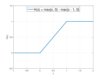
Figure 2: Truncated Hinge-loss with ${\mathbf{a}}=1$ and ${\mathbf{z}}\in\mathbb{R}$

A.2 A Sampling Method to Generate a Stochastic Gradient Estimator

In this subsection, we assume access to an approximate maximizer of $\max_{{\mathbf{z}}\in\mathcal{Z}}\Phi({\mathbf{y}}^{(k)},{\mathbf{z}};{\mathbf{x}}_{i})$ for each $i\in[n]$. Building on this assumption, we construct a specific measure that satisfies Assumption 3, which enables the formulation of a corresponding smoothing function. Subsequently, we demonstrate how to generate a stochastic gradient estimator $\mathcal{G}_{i}({\mathbf{y}}^{(k)},\mu_{k})$ for the specific smoothing function. This estimator, obtained through sampling, satisfies the bias condition in (2.5). Specifically, suppose we can access a point ${\mathbf{z}}^{(k)}_{i}$ such that it is $\frac{\mu_{k}}{8l_{\Psi}}$-close to a global maximizer of problem $\max_{{\mathbf{z}}\in\mathcal{Z}}\Psi({\mathbf{y}}^{(k)},{\mathbf{z}};{\mathbf{x}}_{i})$. We construct $\zeta_{i}^{(k)}$ as the uniform distribution over the ball $\mathcal{B}_{\frac{\mu_{k}}{4l_{\Psi}}}({\mathbf{z}}_{i}^{(k)})$. Consequently, $\zeta:=\zeta_{i}^{(k)}$ satisfies the conditions in Assumption 3. By Lemma 2.4(a), $\mu_{k}\log\mathbb{E}_{{\mathbf{z}}\sim\zeta_{i}^{(k)}}[e^{\Psi(\cdot,{\mathbf{z}};{\mathbf{x}}_{i})/\mu_{k}}]$ is a smoothing function of $\Phi_{i}$ at ${\mathbf{y}}^{(k)}$. To approximate the gradient $\nabla_{{\mathbf{y}}}\widetilde{{\Phi}}_{i}({\mathbf{y}}^{(k)},\mu_{k})$, we generate $M$ i.i.d. samples $\{{\mathbf{z}}_{j}\}_{j=1}^{M}$ from $\zeta_{i}^{(k)}$ and approximate $\widetilde{{\Phi}}_{i}({\mathbf{y}}^{(k)},\mu_{k})$ as

$$\overline{\Phi}_{i}({\mathbf{y}}^{(k)},\mu_{k})=\mu_{k}\log\left(\frac{1}{M}\sum_{j\in\left[M\right]}e^{(\Psi({\mathbf{y}}^{(k)},{\mathbf{z}}_{j};{\mathbf{x}}_{i}))/\mu_{k}}\right).$$

The stochastic gradient estimator is then defined as

$$\mathcal{G}_{i}({\mathbf{y}}^{(k)},\mu_{k}):=\nabla_{{\mathbf{y}}}\overline{\Phi}_{i}({\mathbf{y}}^{(k)},\mu_{k}).$$ (A.1)

Here, $\nabla_{{\mathbf{y}}}\overline{\Phi}_{i}({\mathbf{y}}^{(k)},\mu_{k})$ serves as an approximation of the true gradient $\nabla_{{\mathbf{y}}}\widetilde{{\Phi}}_{i}({\mathbf{y}}^{(k)},\mu_{k})$, with its accuracy improving as $M$ increases.

We establish the following two lemmas, to determine the required sample size $M$ for satisfying condition (2.5) with $\zeta=\zeta_{i}^{(k)}$.

Lemma A.1

Suppose Assumptions 1–4 hold, and we have access to a point ${\mathbf{z}}^{(k)}_{i}$ that is $\frac{\mu_{k}}{8l_{\Psi}}$-close to a global maximizer of problem $\max_{{\mathbf{z}}\in\mathcal{Z}}\Psi({\mathbf{y}}^{(k)},{\mathbf{z}};{\mathbf{x}}_{i})$. Let ${\mathbf{y}}={\mathbf{y}}^{(k)}$, $\mu=\mu_{k}$, and $\zeta=\zeta^{(k)}_{i}$ be the uniform distribution defined as above. Then ${\mathrm{Var}_{{\mathbf{z}}\sim\zeta}\left[e^{\Psi({\mathbf{y}},{\mathbf{z}};{\mathbf{x}}_{i})/\mu}\right]}\leq 3{(\mathbb{E}_{{\mathbf{z}}\sim\zeta}[e^{\Psi({\mathbf{y}},{\mathbf{z}};{\mathbf{x}}_{i})/\mu}])^{2}}$, and $\left\|{\mathrm{Var}_{{\mathbf{z}}\sim\zeta}\left[e^{\Psi({\mathbf{y}},{\mathbf{z}};{\mathbf{x}}_{i})/\mu}\nabla_{{\mathbf{y}}}\Psi({\mathbf{y}},{\mathbf{z}};{\mathbf{x}}_{i})\right]}\right\|\leq 3l_{\Psi}^{2}{(\mathbb{E}_{{\mathbf{z}}\sim\zeta}[e^{\Psi({\mathbf{y}},{\mathbf{z}};{\mathbf{x}}_{i})/\mu}])^{2}}$.

Proof

Since $\zeta$ is the uniform distribution over the ball $\mathcal{B}_{\frac{\mu}{4l_{\Psi}}}({\mathbf{z}}_{i}^{(k)})$, it holds $\|{\mathbf{z}}_{1}-{\mathbf{z}}_{2}\|\leq\frac{\mu}{2l_{\Psi}}$ for all ${\mathbf{z}}_{1},{\mathbf{z}}_{2}\in\mathrm{supp}(\zeta)$. By the $l_{\Psi}$-Lipschitz continuity of $\Psi$ from Assumption 2, we obtain that

$$\max_{{\mathbf{z}}\in\mathrm{supp}(\zeta)}\Psi({\mathbf{y}},{\mathbf{z}};{\mathbf{x}}_{i})-\min_{{\mathbf{z}}\in\mathrm{supp}(\zeta)}\Psi({\mathbf{y}},{\mathbf{z}};{\mathbf{x}}_{i})\leq l_{\Psi}\frac{\mu}{2l_{\Psi}}=\frac{\mu}{2}.$$

Therefore,

$$\frac{{\mathrm{Var}_{{\mathbf{z}}\sim\zeta}\left[e^{\Psi({\mathbf{y}},{\mathbf{z}};{\mathbf{x}}_{i})/\mu}\right]}}{{(\mathbb{E}_{{\mathbf{z}}\sim\zeta}[e^{\Psi({\mathbf{y}},{\mathbf{z}};{\mathbf{x}}_{i})/\mu}])^{2}}}\leq\frac{\mathbb{E}_{{\mathbf{z}}\sim\zeta}[e^{2\Psi({\mathbf{y}},{\mathbf{z}};{\mathbf{x}}_{i})/\mu}]}{{(\mathbb{E}_{{\mathbf{z}}\sim\zeta}[e^{\Psi({\mathbf{y}},{\mathbf{z}};{\mathbf{x}}_{i})/\mu}])^{2}}}\leq{e^{2\left(\max_{{\mathbf{z}}\in\mathrm{supp}(\zeta)}\Psi({\mathbf{y}},{\mathbf{z}};{\mathbf{x}}_{i})-\min_{{\mathbf{z}}\in\mathrm{supp}(\zeta)}\Psi({\mathbf{y}},{\mathbf{z}};{\mathbf{x}}_{i})\right)/\mu}}{}\leq e\leq 3,$$

b where the second inequality uses

$$\mathbb{E}_{{\mathbf{z}}\sim\zeta}[e^{2\Psi({\mathbf{y}},{\mathbf{z}};{\mathbf{x}}_{i})/\mu}]\leq e^{2\max_{{\mathbf{z}}\in\mathrm{supp}(\zeta)}\Psi({\mathbf{y}},{\mathbf{z}};{\mathbf{x}}_{i})/\mu},\text{ and }\mathbb{E}_{{\mathbf{z}}\sim\zeta}[e^{\Psi({\mathbf{y}},{\mathbf{z}};{\mathbf{x}}_{i})/\mu}]\geq e^{\min_{{\mathbf{z}}\in\mathrm{supp}(\zeta)}\Psi({\mathbf{y}},{\mathbf{z}};{\mathbf{x}}_{i})/\mu}.$$

Similarly, using $\left\|\nabla_{{\mathbf{y}}}\Psi({\mathbf{y}},{\mathbf{z}};{\mathbf{x}}_{i})\right\|\leq l_{\Psi}$ from Assumption 2, we have

$$\frac{\left\|{\mathrm{Var}_{{\mathbf{z}}\sim\zeta}\left[e^{\Psi({\mathbf{y}},{\mathbf{z}};{\mathbf{x}}_{i})/\mu}\nabla_{{\mathbf{y}}}\Psi({\mathbf{y}},{\mathbf{z}};{\mathbf{x}}_{i})\right]}\right\|}{{(\mathbb{E}_{{\mathbf{z}}\sim\zeta}[e^{\Psi({\mathbf{y}},{\mathbf{z}};{\mathbf{x}}_{i})/\mu}])^{2}}}\leq \frac{\mathbb{E}_{{\mathbf{z}}\sim\zeta}[e^{2\Psi({\mathbf{y}},{\mathbf{z}};{\mathbf{x}}_{i})/\mu}\left\|\nabla_{{\mathbf{y}}}\Psi({\mathbf{y}},{\mathbf{z}};{\mathbf{x}}_{i})\right\|^{2}]}{{(\mathbb{E}_{{\mathbf{z}}\sim\zeta}[e^{\Psi({\mathbf{y}},{\mathbf{z}};{\mathbf{x}}_{i})/\mu}])^{2}}}$$

$$\leq l_{\Psi}^{2}{e^{2\left(\max_{{\mathbf{z}}\in\mathrm{supp}(\zeta)}\Psi({\mathbf{y}},{\mathbf{z}};{\mathbf{x}}_{i})-\min_{{\mathbf{z}}\in\mathrm{supp}(\zeta)}\Psi({\mathbf{y}},{\mathbf{z}};{\mathbf{x}}_{i})\right)/\mu}}{}\leq 3l_{\Psi}^{2}.$$

The proof is then completed.

Lemma A.2

Under the same assumptions of Lemma A.1, if $M\geq\left\lceil{12l_{\Psi}^{2}\widehat{\epsilon}^{-2}}\right\rceil$, then

$$\mathbb{E}\left\|\mathcal{G}_{i}({\mathbf{y}},\mu)-\nabla_{{\mathbf{y}}}\widetilde{{\Phi}}_{i}({\mathbf{y}},\mu)\right\|^{2}\leq\widehat{\epsilon}^{2}.$$

Proof

For simplicity of notations, let us denote ${\mathbf{y}}={\mathbf{y}}^{(k)}$, $\mu=\mu_{k}$, $\zeta=\zeta^{(k)}_{i}$,

$$\Psi_{1}:=\frac{1}{M}\sum_{j\in\left[M\right]}[e^{\Psi({\mathbf{y}},{\mathbf{z}}_{j};{\mathbf{x}}_{i})/\mu}\nabla_{{\mathbf{y}}}\Psi({\mathbf{y}},{\mathbf{z}}_{j};{\mathbf{x}}_{i})]\mathbb{E}_{{\mathbf{z}}\sim\zeta}[e^{\Psi({\mathbf{y}},{\mathbf{z}};{\mathbf{x}}_{i})/\mu}],\,\,\Psi_{2}:=\frac{1}{M}\sum_{j\in\left[M\right]}[e^{\Psi({\mathbf{y}},{\mathbf{z}}_{j};{\mathbf{x}}_{i})/\mu}]\mathbb{E}_{{\mathbf{z}}\sim\zeta}[e^{\Psi({\mathbf{y}},{\mathbf{z}};{\mathbf{x}}_{i})/\mu}\nabla_{{\mathbf{y}}}\Psi({\mathbf{y}},{\mathbf{z}};{\mathbf{x}}_{i})],$$

$$\text{and }\Psi_{3}:=\frac{1}{M}\sum_{j\in\left[M\right]}[e^{\Psi({\mathbf{y}},{\mathbf{z}}_{j};{\mathbf{x}}_{i})/\mu}]\frac{1}{M}\sum_{j\in\left[M\right]}[e^{\Psi({\mathbf{y}},{\mathbf{z}}_{j};{\mathbf{x}}_{i})/\mu}\nabla_{{\mathbf{y}}}\Psi({\mathbf{y}},{\mathbf{z}}_{j};{\mathbf{x}}_{i})].$$

It holds

$$\mathbb{E}\|\mathcal{G}_{i}({\mathbf{y}},\mu)-\nabla_{{\mathbf{y}}}\widetilde{{\Phi}}_{i}({\mathbf{y}},\mu)\|^{2}$$

$$= \mathbb{E}\left\|\frac{\frac{1}{M}\sum_{j\in\left[M\right]}[e^{\Psi({\mathbf{y}},{\mathbf{z}}_{j};{\mathbf{x}}_{i})/\mu}\nabla_{{\mathbf{y}}}\Psi({\mathbf{y}},{\mathbf{z}}_{j};{\mathbf{x}}_{i})]}{\frac{1}{M}\sum_{j\in\left[M\right]}[e^{\Psi({\mathbf{y}},{\mathbf{z}}_{j};{\mathbf{x}}_{i})/\mu}]}-\frac{\mathbb{E}_{{\mathbf{z}}\sim\zeta}[e^{\Psi({\mathbf{y}},{\mathbf{z}};{\mathbf{x}}_{i})/\mu}\nabla_{{\mathbf{y}}}\Psi({\mathbf{y}},{\mathbf{z}};{\mathbf{x}}_{i})]}{\mathbb{E}_{{\mathbf{z}}\sim\zeta}[e^{\Psi({\mathbf{y}},{\mathbf{z}};{\mathbf{x}}_{i})/\mu}]}\right\|^{2}$$

$$= \mathbb{E}\left\|\frac{\Psi_{1}-\Psi_{2}}{\frac{1}{M}\sum_{j\in\left[M\right]}[e^{\Psi({\mathbf{y}},{\mathbf{z}}_{j};{\mathbf{x}}_{i})/\mu}]\mathbb{E}_{{\mathbf{z}}\sim\zeta}[e^{\Psi({\mathbf{y}},{\mathbf{z}};{\mathbf{x}}_{i})/\mu}]}\right\|^{2}$$

$$\leq 2\mathbb{E}\left\|\frac{\Psi_{1}-\Psi_{3}}{\frac{1}{M}\sum_{j\in\left[M\right]}[e^{\Psi({\mathbf{y}},{\mathbf{z}}_{j};{\mathbf{x}}_{i})/\mu}]\mathbb{E}_{{\mathbf{z}}\sim\zeta}[e^{\Psi({\mathbf{y}},{\mathbf{z}};{\mathbf{x}}_{i})/\mu}]}\right\|^{2}+2\mathbb{E}_{{\mathbf{z}}\sim\zeta}\left\|\frac{\Psi_{3}-\Psi_{2}}{\frac{1}{M}\sum_{j\in\left[M\right]}[e^{\Psi({\mathbf{y}},{\mathbf{z}}_{j};{\mathbf{x}}_{i})/\mu}]\mathbb{E}_{{\mathbf{z}}\sim\zeta}[e^{\Psi({\mathbf{y}},{\mathbf{z}};{\mathbf{x}}_{i})/\mu}]}\right\|^{2}$$

$$\leq 2l^{2}_{\Psi}\mathbb{E}\left\|\frac{\mathbb{E}_{{\mathbf{z}}\sim\zeta}[e^{\Psi({\mathbf{y}},{\mathbf{z}};{\mathbf{x}}_{i})/\mu}]-\frac{1}{M}\sum_{j\in\left[M\right]}[e^{\Psi({\mathbf{y}},{\mathbf{z}}_{j};{\mathbf{x}}_{i})/\mu}]}{\mathbb{E}[e^{\Psi({\mathbf{y}},{\mathbf{z}};{\mathbf{x}}_{i})/\mu}]}\right\|^{2}$$

$$\quad+2\mathbb{E}\left\|\frac{\frac{1}{M}\sum_{j\in\left[M\right]}[e^{\Psi({\mathbf{y}},{\mathbf{z}}_{j};{\mathbf{x}}_{i})/\mu}\nabla_{{\mathbf{y}}}\Psi({\mathbf{y}},{\mathbf{z}}_{j};{\mathbf{x}}_{i})]-\mathbb{E}_{{\mathbf{z}}\sim\zeta}[e^{\Psi({\mathbf{y}},{\mathbf{z}};{\mathbf{x}}_{i})/\mu}\nabla_{{\mathbf{y}}}\Psi({\mathbf{y}},{\mathbf{z}};{\mathbf{x}}_{i})]}{\mathbb{E}_{{\mathbf{z}}\sim\zeta}[e^{\Psi({\mathbf{y}},{\mathbf{z}};{\mathbf{x}}_{i})/\mu}]}\right\|^{2}$$

$$= 2l^{2}_{\Psi}\frac{\mathbb{E}_{{\mathbf{z}}\sim\zeta}\left\|\mathbb{E}_{{\mathbf{z}}\sim\zeta}[e^{\Psi({\mathbf{y}},{\mathbf{z}};{\mathbf{x}}_{i})/\mu}]-\frac{1}{M}\sum_{j\in\left[M\right]}[e^{\Psi({\mathbf{y}},{\mathbf{z}}_{j};{\mathbf{x}}_{i})/\mu}]\right\|^{2}}{(\mathbb{E}_{{\mathbf{z}}\sim\zeta}[e^{\Psi({\mathbf{y}},{\mathbf{z}};{\mathbf{x}}_{i})/\mu}])^{2}}$$

$$\quad+2\frac{\mathbb{E}_{{\mathbf{z}}\sim\zeta}\left\|\frac{1}{M}\sum_{j\in\left[M\right]}[e^{\Psi({\mathbf{y}},{\mathbf{z}}_{j};{\mathbf{x}}_{i})/\mu}\nabla_{{\mathbf{y}}}\Psi({\mathbf{y}},{\mathbf{z}}_{j};{\mathbf{x}}_{i})]-\mathbb{E}_{{\mathbf{z}}\sim\zeta}[e^{\Psi({\mathbf{y}},{\mathbf{z}};{\mathbf{x}}_{i})/\mu}\nabla_{{\mathbf{y}}}\Psi({\mathbf{y}},{\mathbf{z}};{\mathbf{x}}_{i})]\right\|^{2}}{(\mathbb{E}_{{\mathbf{z}}\sim\zeta}[e^{\Psi({\mathbf{y}},{\mathbf{z}};{\mathbf{x}}_{i})/\mu}])^{2}}$$

$$= \frac{2l^{2}_{\Psi}}{M}\frac{{\mathrm{Var}_{{\mathbf{z}}\sim\zeta}\left[e^{\Psi({\mathbf{y}},{\mathbf{z}};{\mathbf{x}}_{i})/\mu}\right]}}{{(\mathbb{E}_{{\mathbf{z}}\sim\zeta}[e^{\Psi({\mathbf{y}},{\mathbf{z}};{\mathbf{x}}_{i})/\mu}])^{2}}}+\frac{2}{M}\frac{\left\|{\mathrm{Var}_{{\mathbf{z}}\sim\zeta}\left[e^{\Psi({\mathbf{y}},{\mathbf{z}};{\mathbf{x}}_{i})/\mu}\nabla_{{\mathbf{y}}}\Psi({\mathbf{y}},{\mathbf{z}};{\mathbf{x}}_{i})\right]}\right\|}{{(\mathbb{E}_{{\mathbf{z}}\sim\zeta}[e^{\Psi({\mathbf{y}},{\mathbf{z}};{\mathbf{x}}_{i})/\mu}])^{2}}}\leq{\frac{12l^{2}_{\Psi}}{M},}$$

where the first inequality uses the triangle inequality, the last one uses Lemma A.1, and the second one holds by

$$\left\|\frac{1}{M}\sum_{j\in\left[M\right]}[e^{\Psi({\mathbf{y}},{\mathbf{z}}_{j};{\mathbf{x}}_{i})/\mu}\nabla_{{\mathbf{y}}}\Psi({\mathbf{y}},{\mathbf{z}}_{j};{\mathbf{x}}_{i})]\right\|^{2}\leq \left(\frac{1}{M}\sum_{j\in\left[M\right]}\left\|e^{\Psi({\mathbf{y}},{\mathbf{z}}_{j};{\mathbf{x}}_{i})/\mu}\nabla_{{\mathbf{y}}}\Psi({\mathbf{y}},{\mathbf{z}}_{j};{\mathbf{x}}_{i})]\right\|\right)^{2}$$

$$\leq \left(\frac{1}{M}\sum_{j\in\left[M\right]}l_{\Psi}\left|e^{\Psi({\mathbf{y}},{\mathbf{z}}_{j};{\mathbf{x}}_{i})/\mu}\right|\right)^{2}=l_{\Psi}^{2}\left(\frac{1}{M}\sum_{j\in\left[M\right]}e^{\Psi({\mathbf{y}},{\mathbf{z}}_{j};{\mathbf{x}}_{i})/\mu}\right)^{2}.$$

The proof is then completed.

Remark A.1

Consider a convex support set $\mathcal{Z}$. Below, we outline two scenarios for accessing an approximate maximizer of $\max_{{\mathbf{z}}\in\mathcal{Z}}\Psi({\mathbf{y}},{\mathbf{z}};{\mathbf{x}}_{i})$.

1. If $\Psi({\mathbf{y}},\cdot;{\mathbf{x}}_{i})$ is concave over $\mathcal{Z}$ for all ${\mathbf{y}}\in\operatorname{dom}(\varphi)$, we can directly access a maximizer using a first-order subgradient method [57]. This method guarantees convergence to a maximizer of $\max_{{\mathbf{z}}\in\mathcal{Z}}\Psi({\mathbf{y}},{\mathbf{z}};{\mathbf{x}}_{i})$, leveraging the concavity of $\Psi$.

2. When a subdifferential error bound condition [24] holds, we can efficiently compute an approximate maximizer. This condition states that, for any ${\mathbf{y}}\in\operatorname{dom}(\varphi)$, there exists a constant $E_{\Psi}>0$ such that for all $i\in[n]$:

   $$\operatorname{dist}({\mathbf{z}},S_{{\mathbf{z}}})\leq E_{\Psi}\cdot\operatorname{dist}(\mathbf{0},\partial_{{\mathbf{z}}}\Psi({\mathbf{y}},{\mathbf{z}};{\mathbf{x}}_{i})),\quad\forall{\mathbf{z}}\in\mathcal{Z},$$

   where $S_{{\mathbf{z}}}$ is the set of maximizers of $\max_{{\mathbf{z}}\in\mathcal{Z}}\Psi({\mathbf{y}},{\mathbf{z}};{\mathbf{x}}_{i})$. Under this condition, at the $k$-th iteration, we can employ a subgradient method [21] to efficiently compute a point ${\mathbf{z}}_{i}^{(k)}\in\mathcal{Z}$ satisfying $\|{\mathbf{z}}_{i}^{(k)}-\bar{{\mathbf{z}}}_{i}^{(k)}\|\leq\frac{\mu}{8l_{\Psi}},$ where $\bar{{\mathbf{z}}}_{i}^{(k)}$ satisfies:

   $$\operatorname{dist}\left(0,\partial_{{\mathbf{z}}}\Psi({\mathbf{y}}^{(k)},\bar{{\mathbf{z}}}_{i}^{(k)};{\mathbf{x}}_{i})+\mathcal{N}_{\mathcal{Z}}(\bar{{\mathbf{z}}}_{i}^{(k)})\right)\leq\frac{\mu}{8l_{\Psi}E_{\Psi}}.$$

   Once ${\mathbf{z}}_{i}^{(k)}$ is obtained, we construct a small ball $\mathcal{B}_{\frac{\mu_{k}}{4l_{\Psi}}}({\mathbf{z}}_{i}^{(k)})$ that contains a maximizer of $\max_{{\mathbf{z}}\in\mathcal{Z}}\Psi({\mathbf{y}},{\mathbf{z}};{\mathbf{x}}_{i})$, as guaranteed by the subdifferential error bound condition.

References

• [1] S. Shafieezadeh Abadeh, P. M. Esfahani, and D. Kuhn. Distributionally robust logistic regression. Advances in Neural Information Processing Systems, 28, 2015.
• [2] L. Adolphs, H. Daneshmand, A. Lucchi, and T. Hofmann. Local saddle point optimization: A curvature exploitation approach. In The 22nd International Conference on Artificial Intelligence and Statistics, pages 486–495. PMLR, 2019.
• [3] I. B. Alexander. Computing the volume, counting integral points, and exponential sums. Discrete & Computational Geometry, 10:123–141, 1992.
• [4] A. Beck and M. Teboulle. Smoothing and first order methods: A unified framework. SIAM Journal on Optimization, 22(2):557–580, 2012.
• [5] W. Bian and X. Chen. Worst-case complexity of smoothing quadratic regularization methods for non-Lipschitzian optimization. SIAM Journal on Optimization, 23(3):1718–1741, 2013.
• [6] W. Bian and X. Chen. Linearly constrained non-Lipschitz optimization for image restoration. SIAM Journal on Imaging Sciences, 8(4):2294–2322, 2015.
• [7] J. Blanchet and Y. Kang. Semi-supervised learning based on distributionally robust optimization. Data Analysis and Applications 3: Computational, Classification, Financial, Statistical and Stochastic Methods, 5:1–33, 2020.
• [8] J. Blanchet, K. Murthy, and F. Zhang. Optimal transport-based distributionally robust optimization: Structural properties and iterative schemes. Mathematics of Operations Research, 47(2):1500–1529, 2022.
• [9] S. P. Boyd and L. Vandenberghe. Convex optimization. Cambridge university press, 2004.
• [10] J. V. Burke, X. Chen, and H. Sun. The subdifferential of measurable composite max integrands and smoothing approximation. Mathematical Programming, 181:229–264, 2020.
• [11] J. V. Burke, T. Hoheisel, and C. Kanzow. Gradient consistency for integral-convolution smoothing functions. Set-Valued and Variational Analysis, 21(2):359–376, 2013.
• [12] X. Chen. Smoothing methods for nonsmooth, nonconvex minimization. Mathematical Programming, 134(1):71–99, 2012.
• [13] Y. Chen, G. Lan, and Y. Ouyang. Optimal primal-dual methods for a class of saddle point problems. SIAM Journal on Optimization, 24(4):1779–1814, 2014.
• [14] Y. Chen, H. Sun, and H. Xu. Decomposition and discrete approximation methods for solving two-stage distributionally robust optimization problems. Computational Optimization and Applications, 78(1):205–238, 2021.
• [15] F. H. Clarke. Optimization and Nonsmooth Analysis. SIAM, Philadelphia, 1990.
• [16] R. Correa and A. Seeger. Directional derivative of a minimax function. Nonlinear Analysis: Theory, Methods & Applications, 9(1):13–22, 1985.
• [17] R. Correa and L. Thibault. Subdifferential analysis of bivariate separately regular functions. Journal of mathematical analysis and applications, 148(1):157–174, 1990.
• [18] Y. Cui and J.-S. Pang. Modern nonconvex nondifferentiable optimization. SIAM, 2021.
• [19] Y. Cui, J.-S. Pang, and B. Sen. Composite difference-max programs for modern statistical estimation problems. SIAM Journal on Optimization, 28(4):3344–3374, 2018.
• [20] C. Daskalakis and I. Panageas. The limit points of (optimistic) gradient descent in min-max optimization. Advances in neural information processing systems, 31, 2018.
• [21] D. Davis and B. Grimmer. Proximally guided stochastic subgradient method for nonsmooth, nonconvex problems. SIAM Journal on Optimization, 29(3):1908–1930, 2019.
• [22] Y. Deng and M. Mahdavi. Local stochastic gradient descent ascent: Convergence analysis and communication efficiency. In International Conference on Artificial Intelligence and Statistics, pages 1387–1395. PMLR, 2021.
• [23] J. Diakonikolas, C. Daskalakis, and M. I. Jordan. Efficient methods for structured nonconvex-nonconcave min-max optimization. In International Conference on Artificial Intelligence and Statistics, pages 2746–2754. PMLR, 2021.
• [24] D. Drusvyatskiy and A. S. Lewis. Error bounds, quadratic growth, and linear convergence of proximal methods. Mathematics of Operations Research, 43(3):919–948, 2018.
• [25] O. Mohajerin Esfahani and D. Kuhn. Data-driven distributionally robust optimization using the Wasserstein metric: Performance guarantees and tractable reformulations. Mathematical Programming, 171(1-2):115–166, 2018.
• [26] T. Fiez and L. J. Ratliff. Local convergence analysis of gradient descent ascent with finite timescale separation. In Proceedings of the International Conference on Learning Representation, 2021.
• [27] R. Gao and A. Kleywegt. Distributionally robust stochastic optimization with Wasserstein distance. Mathematics of Operations Research, 48(2):603–655, 2023.
• [28] I. Goodfellow, Y. Bengio, and A. Courville. Deep learning, volume 1. MIT press Cambridge, 2016.
• [29] I. Goodfellow, J. Shlens, and C. Szegedy. Explaining and harnessing adversarial examples. Preprint, arXiv:1412.6572, 2014.
• [30] B. Grimmer, H. Lu, P. Worah, and V. Mirrokni. The landscape of the proximal point method for nonconvex–nonconcave minimax optimization. Mathematical Programming, pages 1–35, 2022.
• [31] E. Y. Hamedani and N. S. Aybat. A primal-dual algorithm with line search for general convex-concave saddle point problems. SIAM Journal on Optimization, 31(2):1299–1329, 2021.
• [32] R. Huang, B. Xu, D. Schuurmans, and C. Szepesvári. Learning with a strong adversary. Preprint, arXiv:1511.03034, 2015.
• [33] S. Ioffe and C. Szegedy. Batch normalization: Accelerating deep network training by reducing internal covariate shift. Preprint, arXiv:1502.03167, 2015.
• [34] J. Jiang and X. Chen. Optimality conditions for nonsmooth nonconvex-nonconcave min-max problems and generative adversarial networks. Preprint, arXiv:2203.10914, 2022.
• [35] C. Jin, P. Netrapalli, and M. I. Jordan. What is local optimality in nonconvex-nonconcave minimax optimization? In International conference on machine learning, pages 4880–4889. PMLR, 2020.
• [36] L. V. Kantorovich and S. G. Rubinshtein. On a space of totally additive functions. Vestnik of the St. Petersburg University: Mathematics, 13(7):52–59, 1958.
• [37] W. Kong and R. D. C. Monteiro. An accelerated inexact proximal point method for solving nonconvex-concave min-max problems. SIAM Journal on Optimization, 31(4):2558–2585, 2021.
• [38] D. Kuhn, P. M. Esfahani, V. A. Nguyen, and S. Shafieezadeh Abadeh. Wasserstein distributionally robust optimization: Theory and applications in machine learning. In Operations research & management science in the age of analytics, pages 130–166. Informs, 2019.
• [39] D. Kuhn, S. Shafiee, and W. Wiesemann. Distributionally robust optimization, 2024.
• [40] G. Lan and Y. Li. A novel catalyst scheme for stochastic minimax optimization. Preprint, arXiv:2311.02814, 2023.
• [41] Y. LeCun, Y. Bengio, and G. Hinton. Deep learning. nature, 521(7553):436–444, 2015.
• [42] J. Li, S. Huang, and A. M.-C. So. A first-order algorithmic framework for distributionally robust logistic regression. Advances in Neural Information Processing Systems, 32, 2019.
• [43] J. Li, L. Zhu, and A. M.-C. So. Nonsmooth composite nonconvex-concave minimax optimization. Preprint, arXiv:2209.10825, 2022.
• [44] H. Liang, B. Liang, L. Peng, Y. Cui, T. Mitchell, and J. Sun. Optimization and optimizers for adversarial robustness. Preprint, arXiv:2303.13401, 2023.
• [45] H. Liang, B. Liang, J. Sun, Y. Cui, and T. Mitchell. Implications of solution patterns on adversarial robustness. In Proceedings of the IEEE/CVF Conference on Computer Vision and Pattern Recognition, pages 2393–2400, 2023.
• [46] T. Lin, C. Jin, and M. I. Jordan. Near-optimal algorithms for minimax optimization. In Conference on Learning Theory, pages 2738–2779. PMLR, 2020.
• [47] T. Lin, C. Jin, and M. I. Jordan. On gradient descent ascent for nonconvex-concave minimax problems. In International Conference on Machine Learning, pages 6083–6093. PMLR, 2020.
• [48] M. Liu, H. Rafique, Q. Lin, and T. Yang. First-order convergence theory for weakly-convex-weakly-concave min-max problems. The Journal of Machine Learning Research, 22(1):7651–7684, 2021.
• [49] Y. Liu, X. Yuan, and J. Zhang. Discrete approximation scheme in distributionally robust optimization. Numer Math Theory Methods Appl, 14(2):285–320, 2021.
• [50] S. Lu, I. Tsaknakis, M. Hong, and Y. Chen. Hybrid block successive approximation for one-sided non-convex min-max problems: algorithms and applications. IEEE Transactions on Signal Processing, 68:3676–3691, 2020.
• [51] A. Madry, A. Makelov, L. Schmidt, D. Tsipras, and A. Vladu. Towards deep learning models resistant to adversarial attacks. Preprint, arXiv:1706.06083, 2017.
• [52] A. Madry, A. Makelov, L. Schmidt, D. Tsipras, and A. Vladu. Towards deep learning models resistant to adversarial attacks. In International Conference on Learning Representations, 2018.
• [53] G. Mancino-Ball and Y. Xu. Variance-reduced accelerated methods for decentralized stochastic double-regularized nonconvex strongly-concave minimax problems. Preprint, arXiv:2307.07113, 2023.
• [54] E. V. Mazumdar, M. I. Jordan, and S. S. Sastry. On finding local nash equilibria (and only local nash equilibria) in zero-sum games. Preprint, arXiv:1901.00838, 2019.
• [55] R. Mifflin. Semismooth and semiconvex functions in constrained optimization. SIAM J. Control Optim., 15(6):959–972, 1977.
• [56] A. M. Mood. Introduction to the theory of statistics. 1950.
• [57] Y. Nesterov. Primal-dual subgradient methods for convex problems. Mathematical programming, 120(1):221–259, 2009.
• [58] M. Nouiehed, M. Sanjabi, T. Huang, J. D. Lee, and M. Razaviyayn. Solving a class of non-convex min-max games using iterative first order methods. Advances in Neural Information Processing Systems, 32, 2019.
• [59] J.-S. Pang, M. Razaviyayn, and A. Alvarado. Computing B-stationary points of nonsmooth dc programs. Mathematics of Operations Research, 42(1):95–118, 2017.
• [60] E. Y. Pee and J. O. Royset. On solving large-scale finite minimax problems using exponential smoothing. Journal of optimization theory and applications, 148(2):390–421, 2011.
• [61] G. Pflug and D. Wozabal. Ambiguity in portfolio selection. Quantitative Finance, 7(4):435–442, 2007.
• [62] E. Polak, J. O. Royset, and R. S. Womersley. Algorithms with adaptive smoothing for finite minimax problems. Journal of Optimization Theory and Applications, 119:459–484, 2003.
• [63] H. Rafique, M. Liu, Q. Lin, and T. Yang. Weakly-convex–concave min–max optimization: provable algorithms and applications in machine learning. Optimization Methods and Software, 37(3):1087–1121, 2022.
• [64] H. Rahimian and S. Mehrotra. Distributionally robust optimization: A review. Preprint, arXiv:1908.05659, 2019.
• [65] R. T. Rockafellar and R. J.-B. Wets. Variational Analysis. Springer Science $\&$ Business Media, 1998.
• [66] L. Sangyoon, K. Hyunwoo, and M. Ilkyeong. A data-driven distributionally robust newsvendor model with a Wasserstein ambiguity set. Journal of the Operational Research Society, 72(8):1879–1897, 2021.
• [67] A. Selvi, M. R. Belbasi, M. Haugh, and W. Wiesemann. Wasserstein logistic regression with mixed features. Advances in Neural Information Processing Systems, 35:16691–16704, 2022.
• [68] A. Shapiro, D. Dentcheva, and A. Ruszczynski. Lectures on stochastic programming: modeling and theory. SIAM, 2021.
• [69] A. Sinha, H. Namkoong, and J. Duchi. Certifiable distributional robustness with principled adversarial training. In International Conference on Learning Representations, 2018.
• [70] J. T. Springenberg, A. Dosovitskiy, T. Brox, and M. Riedmiller. Striving for simplicity: The all convolutional net. Preprint, arXiv:1412.6806, 2014.
• [71] K. K. Thekumparampil, P. Jain, P. Netrapalli, and S. Oh. Efficient algorithms for smooth minimax optimization. Advances in Neural Information Processing Systems, 32, 2019.
• [72] J. von Neumann. Zur theorie der gesellschaftsspiele. Mathematische annalen, 100(1):295–320, 1928.
• [73] J. Wang, R. Gao, and Y. Xie. Sinkhorn distributionally robust optimization. Preprint, arXiv:2109.11926, 2021.
• [74] R. Wang and C. Zhang. Stochastic smoothing accelerated gradient method for nonsmooth convex composite optimization. Preprint, arXiv:2308.01252, 2023.
• [75] Y. Wang, G. Zhang, and J. Ba. On solving minimax optimization locally: A follow-the-ridge approach. In International Conference on Learning Representations, 2020.
• [76] D. Wozabal. A framework for optimization under ambiguity. Annals of Operations Research, 193(1):21–47, 2012.
• [77] H. Xu, Y. Liu, and H. Sun. Distributionally robust optimization with matrix moment constraints: Lagrange duality and cutting plane methods. Mathematical programming, 169:489–529, 2018.
• [78] Y. Xu. Decentralized gradient descent maximization method for composite nonconvex strongly-concave minimax problems. SIAM Journal on Optimization, 34(1):1006–1044, 2024.
• [79] Z. Xu, H. Zhang, Y. Xu, and G. Lan. A unified single-loop alternating gradient projection algorithm for nonconvex–concave and convex–nonconcave minimax problems. Mathematical Programming, pages 1–72, 2023.
• [80] Y. Yan and Y. Xu. Adaptive primal-dual stochastic gradient method for expectation-constrained convex stochastic programs. Mathematical Programming Computation, 14(2):319–363, 2022.
• [81] J. Yang, N. Kiyavash, and N. He. Global convergence and variance-reduced optimization for a class of nonconvex-nonconcave minimax problems. Preprint, arXiv:2002.09621, 2020.
• [82] J. Yang, A. Orvieto, A. Lucchi, and N. He. Faster single-loop algorithms for minimax optimization without strong concavity. In International Conference on Artificial Intelligence and Statistics, pages 5485–5517. PMLR, 2022.
• [83] M.-C. Yue, D. Kuhn, and W. Wiesemann. On linear optimization over Wasserstein balls. Mathematical Programming, 195(1-2):1107–1122, 2022.
• [84] C. Zhang, M. Pham, S. Fu, and Y. Liu. Robust multicategory support vector machines using difference convex algorithm. Mathematical programming, 169:277–305, 2018.
• [85] S. Zhang, Y. Hu, L. Zhang, and N. He. Generalization bounds of nonconvex-(strongly)-concave stochastic minimax optimization. In International Conference on Artificial Intelligence and Statistics, pages 694–702. PMLR, 2024.
• [86] X. Zhang, N. S. Aybat, and M. Gurbuzbalaban. Sapd+: An accelerated stochastic method for nonconvex-concave minimax problems. Advances in Neural Information Processing Systems, 35:21668–21681, 2022.
• [87] X. Zhang, G. Mancino-Ball, N. S. Aybat, and Y. Xu. Jointly improving the sample and communication complexities in decentralized stochastic minimax optimization. In Proceedings of the AAAI Conference on Artificial Intelligence, volume 38, pages 20865–20873, 2024.
• [88] R. Zhao. Accelerated stochastic algorithms for convex-concave saddle-point problems. Mathematics of Operations Research, 47(2):1443–1473, 2022.
• [89] R. Zhao. A primal-dual smoothing framework for max-structured non-convex optimization. Mathematics of operations research, 49(3):1535–1565, 2024.