Model-Based Learning for DOA Estimation with One-Bit Single-Snapshot Sparse Arrays

Abstract

We address the challenging problem of estimating the directions-of-arrival (DOAs) of multiple off-grid signals using a single snapshot of one-bit quantized measurements. Conventional DOA estimation methods face difficulties in tackling this problem effectively. This paper introduces a domain-knowledge-guided learning framework to achieve high-resolution DOA estimation in such a scenario, thus drastically reducing hardware complexity without compromising performance. We first reformulate DOA estimation as a maximum a posteriori (MAP) problem, unifying on-grid and off-grid scenarios under a Laplacian-type sparsity prior to effectively enforce sparsity for both uniform and sparse linear arrays. For off-grid signals, a first-order approximation grid model is embedded into the one-bit signal model. We then reinterpret one-bit sensing as a binary classification task, employing a multivariate Bernoulli likelihood with a logistic link function to enhance stability and estimation accuracy. To resolve the non-convexity inherent in the MAP formulation, we develop augmented algorithmic frameworks based on majorization-minimization principles. Further, we design model-based inference neural networks by deep unrolling these frameworks, significantly reducing computational complexity while preserving the estimation precision. Extensive simulations demonstrate the robustness of the proposed framework across a wide range of input signal-to-noise ratio values and off-grid deviations. By integrating the unified model-based priors with data-driven learning, this work bridges the gap between theoretical guarantees and practical feasibility in one-bit single-snapshot DOA estimation, offering a scalable, hardware-efficient solution for next-generation radar and communication systems.

I Introduction

Direction-of-arrival (DOA) estimation is fundamentally important in sensor array signal processing with wide application in radar, sonar, navigation, and wireless communications[2, 3, 4, 5, 6]. Commonly used super-resolution DOA estimation algorithms, such as MUltiple SIgnal Classification (MUSIC) [7] and estimation of signal parameters via rotational invariant techniques (ESPRIT) [8], often assume a uniform linear array (ULA) configuration, where sensor elements are arranged in a straight line with equal spacing, typically half the signal wavelength. However, in practical applications, achieving higher resolution with large-size ULA requires a substantial number of array elements, significantly increasing hardware costs[6]. Furthermore, ULAs are susceptible to mutual coupling effects, which can degrade DOA estimation performance[9]. To address this problem, sparse linear arrays (SLAs) have been used over the past few decades to achieve desired apertures with fewer active elements. Some SLA configurations, such as the minimum redundancy array (MRA)[10], the nested array[11], the co-prime array[12], the generalized coprime array configurations [13], and the maximum inter-element spacing constraint (MISC) [14], have been well studied and analyzed in the past decades. Although subspace-based methods, such as MUSIC and weighted subspace fitting [15], and covariance matrix-based compressive sensing methods [16] can be applied to SLAs exploiting difference coarrays, they require a high number of snapshots to achieve accurate covariance matrix estimation, making them impractical in snapshot-limited scenarios commonly encountered in automotive applications [4].

In antenna array systems, high-precision, high-sampling-rate analog-to-digital converters (ADCs) are costly and power-intensive. One-bit quantization provides a cost-effective solution, simplifying the sampling hardware and lowering the sampling rates by reducing the number of bits per sample to just one [17]. Consequently, one-bit signal processing has drawn significant research interest in many fields. In communications, a novel framework for computing the minimum mean square error (MMSE) channel estimator in one-bit quantized multi-input multi-output (MIMO) systems was developed in [18]. In [19], a two-stage detection method for massive MIMO with one-bit ADCs was proposed, which employs Bussgang-based linear receivers and a model-driven neural network, achieving robust performance at significantly reduced complexity. In [20], a novel one-bit MIMO precoding scheme was proposed using spatial Sigma-Delta modulation to effectively control quantization errors utilizing favorable conditions of a massive MIMO system. In the field of radar signal processing, target parameter estimation based on one-bit quantized measurements has emerged as a prominent research topic [21, 22, 23]. In [24], one-bit ADC radar parameter estimation was formulated as a cyclic multivariate weighted least squares problem. A dimension-reduced generalized approximate message passing approach was introduced in [25] for one-bit frequency-modulated continuous-wave (FMCW) radar that mitigates high-order harmonic interference. Multiple sparse recovery algorithms were extended in [26] to a one-bit quantization setting, resulting in one-bit sparse learning via iterative minimization (1bSLIM), likelihood-based estimation of sparse parameters (1bLIKES), one-bit sparse iterative covariance-based estimation (1bSPICE), and one-bit iterative adaptive approaches (1bIAA), to generate automotive radar range-Doppler imaging exploiting one-bit quantization.

I-A Relevant Works

Subspace-based methods exploiting one-bit quantized data, along with performance analyses, were presented for both ULAs and SLAs [2, 27, 28]. It is shown in [2] that the identifiability of one-bit DOA estimation with SLAs matches unquantized measurements and a conservative Cramér-Rao bound (CRB) for quantized systems is derived. In [28], MUSIC-based DOA estimation leverages an approximate one-bit covariance matrix, derived as a scaled version of the unquantized covariance matrix. In the past decade, methods leveraging sparse reconstruction [29] and compressed sensing (CS) [30] have emerged to address one-bit DOA estimation and sparse sensing, leading to various estimators, such as binary iterative hard thresholding (BIHT) [31], robust one-bit Bayesian compressed sensing (R1BCS) [32]. The generalized sparse Bayesian learning (Gr-SBL) algorithm for both single- and multi-snapshot scenarios [33] can operate effectively with SLAs. However, all these methods only consider on-grid signals, as they determine signal DOAs by peak searching over a fixed discrete angular spectrum.

For off-grid signals, grid refinement is commonly employed to maintain estimation accuracy, but it requires denser grids, increasing computational complexity. In CS-based methods, denser grids also lead to higher correlations among dictionary atoms, thereby degrading algorithm performance. To overcome these challenges, gridless and off-grid estimation methods have been developed to tackle the one-bit off-grid DOA estimation problem. Gridless methods, such as atomic norm minimization (ANM) [34], estimate DOAs without grid division but require solving a computationally intensive semidefinite programming (SDP) problem. On the other hand, off-grid methods, such as the off-grid iterative reweighted (OGIR) algorithm [35], alternatively refine on-grid spectrum estimates and grid-gap estimates to enhance estimation accuracy. In [36], an improved root SBL (IRSBL) method was developed for off-grid DOA estimation that refines a coarse initial dictionary through polynomial rooting and extends its applicability to nonuniform linear arrays. Off-grid methods generally eliminate the need for dense grid division, making them more flexible and applicable for real-world DOA estimation tasks compared to gridless methods. However, these methods often require hundreds of iterations to converge, with each iteration involving computationally expensive matrix inversion.

In recent years, deep learning has emerged as a powerful tool in DOA estimation, due to its ability to learn complex patterns and representations from data [37]. However, classical purely data-driven deep neural network-based methods often lack interpretability, and their generalization ability is largely dependent on the size and diversity of the training dataset. Recently, model-based deep learning has gained significant traction in the signal processing community [38, 39], including its applications in DOA estimation research [40, 41, 42, 43]. For array signal processing, model-based deep learning approaches leverage domain knowledge to combine the strengths of traditional signal processing models with the flexibility of deep learning, thus effectively overcoming the limitations of purely data-driven methods and improving performance. In addition, hybrid approaches combine the interpretability of classical array signal models with the representation power of deep neural networks, thus better addressing limitations of traditional signal processing methods in handling high-dimensional, noisy, or complex data. For example, in [44], the authors successfully demonstrated that a learned iterative shrinkage-thresholding algorithm (LISTA) based framework provides superior DOA estimation capability using a limited number of one-bit quantized measurements.

I-B Contributions

In this paper, to tackle DOA estimation in a single-snapshot one-bit quantized antenna array, we propose a learning-augmented framework that unifies model-based optimization with data-driven neural networks. At its core, our methodology leverages a maximum a posteriori (MAP) estimation approach, reformulating one-bit DOA estimation as a sparsity-constrained inverse problem. Unlike existing sparse recovery techniques, we adopt a Laplacian-type prior [45] to enforce structural sparsity, allowing robust recovery of both on-grid and off-grid signals. For off-grid scenarios, a first-order approximation grid model is integrated into the one-bit signal model, thus bypassing the need for iterative grid refinement and ensuring computational tractability for both ULAs and SLAs. To mitigate the non-convexity inherent in one-bit MAP estimation, we employ a majorization-minimization (MM) approach to construct a surrogate convex function, which serves as a substitute for the original objective function, facilitating more efficient optimization. In addition to using the Gaussian cumulative distribution function (CDF) as the likelihood function in MAP estimation, the problem is also reformulated as a binary classification task, where the likelihood follows a multivariate Bernoulli distribution with a logistic link function. This approach offers advantages such as differentiability, computational efficiency, and seamless integration into deep neural network architectures. Finally, the iterative algorithms derived from this framework are distilled into a deep-unrolled neural network, which reduces computational complexity by unrolling optimization steps into a feedforward architecture while preserving estimation accuracy. This codesign of model-based priors and learning-based inference bridges theoretical guarantees with practical efficiency, enabling real-time deployment in resource-constrained systems.

Our main contributions are summarized as follows.

• We formulate one-bit DOA estimation problems using a sparse Bayesian framework and the MAP estimation approach with a Laplacian-type prior to enforce sparsity. A first-order approximation grid model is integrated into the one-bit signal model for off-grid DOA estimation, offering a more practical and easily implementable framework for algorithm derivation.

• We introduce an augmented sparse Bayesian framework that reimagines one-bit DOA estimation as a binary classification task. By modeling likelihood as a multivariate Bernoulli distribution with a logistic link function, this approach achieves computational efficiency and differentiability, enabling seamless integration into deep neural networks. We employ an MM approach to mitigate the non-convexity in the augmented one-bit MAP estimator.

• We propose a one-bit DOA inference neural network that synergizes model-based sparse priors with learning-based optimization, harnessing the deep-unrolling paradigm to slash computational complexity while maintaining estimation accuracy. This model-based architecture ensures interpretability inherent to model-driven methods and sustains robustness across broad SNR regimes, bridging the gap between theoretical guarantees and real-world deployment in low-resolution array systems.

In [1], a baseline model-based network was introduced for one-bit off-grid DOA estimation. In this paper, our work further advances the field through multiple key innovations. First, we propose an augmented Bayesian framework that generalizes the likelihood model to a multivariate Bernoulli distribution with a logistic link function, enabling gradient-based optimization and seamless integration with deep neural networks. Second, we employ an MM approach to mitigate the non-convexity inherent in the augmented one-bit MAP estimator. Third, the model-based learning framework is extensively evaluated concerning state-of-the-art approaches.

The rest of the paper is organized as follows. Section II introduces the one-bit DOA estimation signal model and provides a mathematical formulation for both on-grid and off-grid cases. In Section III, we derive two algorithm frameworks SBRI and SBRI-X for one-bit DOA estimation, based on the Sparse Bayesian Reweighted Iterative approach, addressing both on-grid and off-grid DOA estimation. Section IV presents model-based neural networks inspired by algorithm unrolling. Section V provides numerical results for performance evaluation. Finally, Section VI concludes the paper.

We adopt the following notation throughout the paper. Scalars are denoted by lowercase lightface letters, vectors by lowercase boldface letters, and matrices by uppercase boldface letters. $(\cdot)^{\rm T}$, $(\cdot)^{\rm H}$, $(\cdot)^{*}$ respectively represent the transpose, Hermitian, and conjugation operations. $\Re(\cdot)$ and $\Im(\cdot)$ respectively return the real and imaginary parts of complex values. $\mathrm{sign}\left(\cdot\right)$ denotes the sign function with $\mathrm{sign}\left(x\right)=1$ for $x\geq 0$ and $\mathrm{sign}\left(x\right)=-1$ for $x<0$, whereas $\mathrm{csgn}\left(\cdot\right)=\mathrm{sign}(\Re\left(\cdot\right))+j\mathrm{sign}\left(\Im\left(\cdot\right)\right)$ is the complex sign function. Symbol $\odot$ is an element-wise Hadamard product, and $\mathrm{diag}(\cdot)$ represents the operation that diagonalizes the input.

II System Model

Consider a scenario involving $K$ narrowband, far-field signals, represented as $s_{k}(t)$ for $k=1,\dots,K$, impinging on an $M$-element SLA from directions $\bm{\theta}=[\theta_{1},\cdots,\theta_{K}]^{\mathrm{T}}$. As we focus on single-snapshot DOA estimation, the array signal model with one-bit quantization data is presented as:

$$\overline{\mathbf{y}} =\mathrm{csgn}\left(\mathbf{y}\right)=\mathrm{csgn}\big{(}\mathbf{A}(\bm{\theta})\mathbf{s}+\mathbf{n}\big{)},$$ (1)

where $\mathbf{y}\in\mathbb{C}^{M\times 1}$ is the received signal vector and $\overline{\mathbf{y}}\in\mathbb{C}^{M\times 1}$ is its one-bit quantized version, $\mathbf{A}(\bm{\theta})=\left[\mathbf{a}(\theta_{1}),\mathbf{a}(\theta_{2}),\dots,\mathbf{a}(\theta_{K})\right]\in\mathbb{C}^{M\times K}$ is the SLA manifold matrix, $\mathbf{s}=[s_{1},\cdots,s_{K}]^{\mathrm{T}}\in\mathbb{C}^{K\times 1}$ is the impinging signal vector, and $\mathbf{n}\in\mathbb{C}^{M\times 1}$ is the complex additive noise vector. Each column vector in the array manifold matrix $\mathbf{A}(\bm{\theta})$ is a steering vector, given for the $k$-th signal DOA as:

$$\mathbf{a}(\theta_{k})=\left[1,e^{j\frac{2\pi d_{2}}{\lambda}\sin{\theta_{k}}},\dots,e^{j\frac{2\pi d_{M}}{\lambda}\sin{\theta_{k}}}\right]^{\mathrm{T}},$$ (2)

where $d_{m}$, $m=2,\cdots,M$, denote the spacing between the $m$-th SLA element and the first element, and $\lambda$ is wavelength.

II-A On-Grid Single-Measurement Vector Model

To estimate $\bm{\theta}$ from $\left(\ref{signle_snapshot_one_bit_data_model}\right)$, we first construct a classic single-measurement vector model using $N$ grid points:

$$\overline{\mathbf{y}}=\mathrm{csgn}(\mathbf{\mathcal{A}}\mathbf{x}+\mathbf{n}),$$ (3)

where $\mathbf{\mathcal{A}}=[\mathbf{a}(\tilde{\theta}_{1}),\mathbf{a}(\tilde{\theta}_{2}),\dots,\mathbf{a}(\tilde{\theta}_{N})]\in\mathbb{C}^{M\times N}$ is the dictionary matrix with $N\gg M>K$, $\mathbf{a}(\tilde{\theta}_{i})\in\mathbb{C}^{M\times 1}$ is a dictionary atom, where the elements of $\bm{\Theta}=\{\tilde{\theta}_{1},\tilde{\theta}_{2},\dots,\tilde{\theta}_{N}\}\in\mathbb{R}^{N\times 1}$ are obtained from uniform angle-space division, and $\mathbf{x}=\left[x_{1},x_{2},\dots,x_{N}\right]^{\mathrm{T}}\in\mathbb{R}^{N\times 1}$ defines the dictionary atom coefficients to be estimated. Under this model, the $N$ grid points form the bases for sparse signal representation. When the signal can be expressed by using exactly $K$ bases, i.e., $\theta_{k}\in\bm{\Theta}$, $\forall\ k=1,\cdots,K$, this model is referred to as an on-grid model.

II-B Off-Grid Single-Measurement Vector Model

In practice, however, it is unlikely that the pre-demarcated grid corresponds exactly to all signal DOAs, i.e., $\theta_{k}\notin\Theta$ for some or all $K$ signals. Assume the grid is sufficiently dense such that the $K$ signals fall within distinct grid regions, and we denote the fixed grid point closest to the true DOA $\theta_{k}$ as $\tilde{\theta}_{n_{k}}$, $n_{k}\in\left\{1,2,\dots,N\right\}$. Then, the true DOA can be expressed as:

$$\theta_{k}=\tilde{\theta}_{n_{k}}+(\theta_{k}-\tilde{\theta}_{n_{k}}),$$ (4)

where $(\theta_{k}-\tilde{\theta}_{n_{k}})$ represents the grid-gap between the fixed grid point and the true DOA. Using a first-order Taylor expansion, the steering vector $\mathbf{a}(\theta_{k})$ can be approximated as:

$$\hat{\mathbf{a}}(\theta_{k})=\mathbf{a}(\tilde{\theta}_{n_{k}})+\mathbf{b}(\tilde{\theta}_{n_{k}})(\theta_{k}-\tilde{\theta}_{n_{k}}),$$ (5)

where $\mathbf{b}(\tilde{\theta}_{n_{k}})=\frac{\partial\bm{a}(\theta)}{\partial\theta}|_{\tilde{\theta}_{n_{k}}}\in\mathbb{C}^{M\times 1}$ is the first-order derivative of $\bm{a}(\theta)$ at $\tilde{\theta}_{n_{k}}$. In this case, the dictionary matrix is approximated as $\mathbf{C}(\bm{\beta})=\mathbf{\mathcal{A}}+\mathbf{\mathcal{B}}\mathrm{diag}\left(\bm{\beta}\right)$, where $\mathcal{B}=[\mathbf{b}(\tilde{\theta}_{1}),\mathbf{b}(\tilde{\theta}_{2}),\dots,\mathbf{b}(\tilde{\theta}_{N})]\in\mathbb{C}^{M\times N}$, and the elements of $\bm{\beta}=\left[\beta_{1},\beta_{2},\dots,\beta_{N}\right]^{\mathrm{T}}$ are off-grid gaps, defined as:

$$\beta_{n}=\begin{cases}\theta_{k}-\tilde{\theta}_{n_{k}},\ \textrm{if}\ n=n_{k},k\in\left\{1,2,...,K\right\},\\ 0,\ \hskip 30.00005pt\textrm{otherwise}.\end{cases}$$ (6)

By including the approximation error in the measurement noise, the measurement model in (3) can be reformulated as:

$$\overline{\mathbf{y}}=\mathrm{csgn}\big{(}\mathbf{C}(\bm{\beta})\mathbf{x}+\mathbf{n}\big{)}.$$ (7)

III Sparse Bayesian Learning Framework for One-Bit DOA Estimation

In this section, we introduce a sparse Bayesian reweighted iterative (SBRI) framework and its augmented variant for the estimation of on-grid and off-grid signal DOAs based on one-bit quantized array data.

III-A One-Bit On-Grid DOA Estimation via SBRI Framework

We first introduce a probabilistic model to characterize the relationship between unknown atom coefficient vector $\mathbf{x}$ and the observed input $\overline{\mathbf{y}}$. Based on (7), the posterior probability of $\mathbf{x}$ under the MAP criterion is primarily determined by the likelihood function $p\left(\overline{\mathbf{y}}|\mathbf{x};\bm{\beta}\right)$ and the prior probability density function (PDF) $p\left(\mathbf{x}\right)$. The denominator of the posterior density is ignored as it is a positive constant that has no impact on the optimization process. It is assumed that the noise vector $\mathbf{n}$ contains independent and identically distributed (i.i.d.) complex Gaussian elements, denoted as $\mathbf{n}\sim\mathcal{CN}(0,\sigma^{2}\mathbf{I})$.

For the on-grid model described in (1), the likelihood function is given by[46, 26]:

$$p\left(\overline{\mathbf{y}}|\mathbf{x}\right)=\prod_{m=1}^{M} \Phi\left(\frac{\Re\left(\overline{y}_{m}\right)\Re(\mathbf{a}_{m}^{\mathrm{T}}\mathbf{x})}{\sigma/\sqrt{2}}\right)\Phi\left(\frac{\Im\left(\overline{y}_{m}\right)\Im(\mathbf{a}_{m}^{\mathrm{T}}\mathbf{x})}{\sigma/\sqrt{2}}\right),$$ (8)

where $\Phi\left(\cdot\right)$ denotes the CDF of the standard normal distribution, $\overline{y}_{m}$ is the $m$-th element in $\mathbf{y}$, $\mathbf{a}_{m}^{\mathrm{T}}$ is the $m$-th row vector in $\mathbf{\mathcal{A}}$. Since $\sigma>0$ and scaling $\mathbf{x}$ by a positive constant does not affect the values of $\overline{\bm{y}}$ or the DOA estimation results, letting $\hat{\mathbf{x}}=\frac{\sqrt{2}}{\sigma}\mathbf{x}$, (8) is reformulated as:

$$p\left(\overline{\mathbf{y}}|\hat{\mathbf{x}}\right)=\!\prod_{m=1}^{M} \Phi\left(\Re(\overline{y}_{m})\Re(\bm{a}_{m}^{\mathrm{T}}\hat{\mathbf{x}})\right)\Phi\left(\Im(\overline{y}_{m})\Im(\bm{a}_{m}^{\mathrm{T}}\hat{\mathbf{x}})\right).$$ (9)

To promote sparsity in $\hat{\mathbf{x}}$, an appropriate prior PDF is required. We adopt a Laplacian-inspired prior PDF defined as [45]:

$$p\left(\hat{\mathbf{x}}\right)=\prod_{i=1}^{N}\mathrm{exp}\left(-\frac{\gamma\left|\hat{x}_{i}\right|^{\alpha}}{\alpha}\right),\ \ 0<\alpha\leq 1,$$ (10)

where the parameter $\gamma>0$. As $\alpha$ approaches $0$, $p\left(\hat{\mathbf{x}}\right)$ sharply peaks at $\hat{\mathbf{x}}=0$, enforcing sparsity on the estimated $\hat{\mathbf{x}}$. Notice that, if we choose the prior PDF as $p\left(\hat{\mathbf{x}}\right)=\frac{1}{\left|\hat{\mathbf{x}}\right|^{2}+\varepsilon}$, where $\varepsilon>0$ is a small constant, we will derive the 1bSLIM approach proposed in [26]. Using Bayes’ rule, the MAP estimator for on-grid model is given as:

$$\hat{\mathbf{x}}^{\star}=\mathrm{arg}\min_{\hat{\mathbf{x}}}\bigg{\{}-\mathrm{ln}\,p\left(\overline{\mathbf{y}}|\hat{\mathbf{x}}\right)-\mathrm{ln}\,p\left(\hat{\mathbf{x}}\right)\bigg{\}}.$$ (11)

Substituting (8) and (10) into equation (11), we obtain the following cost function to be minimized:

$$\mathcal{L}_{\mathrm{ongrid}} =\sum_{m=1}^{M}\Bigg{\{}-\mathrm{ln}\,\Phi\left(\Re\left(\overline{y}_{m}\right)\Re(\bm{a}_{m}^{\mathrm{T}}\hat{\mathbf{x}})\right)$$

$$\ \ -\mathrm{ln}\,\Phi\left(\Im\left(\overline{y}_{m}\right)\Im(\bm{a}_{m}^{\mathrm{T}}\hat{\mathbf{x}})\right)+\sum_{i=1}^{N}\frac{\gamma\left|x_{i}\right|^{\alpha}}{\alpha}+\textrm{const}\Bigg{\}}.$$ (12)

Since $\mathcal{L}_{\mathrm{ongrid}}$ in (12) is non-convex, we apply convex relaxation to make it more tractable. Specifically, using the MM principle and following the derivations given in [26, 47], we find the upper bound of the first two terms in (12) as:

$$\sum_{m=1}^{M}\!\left\{\!-\mathrm{ln}\,\Phi\left(\Re\left(\overline{y}_{m}\right)\!\Re(\bm{a}_{m}^{\mathrm{T}}\hat{\mathbf{x}})\right)\!-\!\mathrm{ln}\,\Phi\left(\Im\left(\overline{y}_{m}\right)\!\Im(\bm{a}_{m}^{\mathrm{T}}\hat{\mathbf{x}})\right)\!\right\}$$

$$\leq \sum_{m=1}^{M}\bigg{\{}\frac{1}{2}\left(\Re\left(\overline{y}_{m}\right)\Re(\bm{a}_{m}^{\mathrm{T}}\hat{\mathbf{x}})\right)^{2}\!+\frac{1}{2}\left(\Im(\overline{y}_{m})\Im(\bm{a}_{m}^{\mathrm{T}}\hat{\mathbf{x}})\right)^{2}$$

$$-\Re(v_{m}^{k})\Re(\overline{y}_{m})\Re(\bm{a}_{m}^{\mathrm{T}}\hat{\mathbf{x}})\!-\!\Im(v_{m}^{k})\Im(\overline{y}_{m})\Im(\bm{a}_{m}^{\mathrm{T}}\hat{\mathbf{x}})+c^{\prime}\bigg{.}\bigg{\}},$$ (13)

where $v_{m}^{k}=\left[\Re(\overline{y}_{m})\Re(\tilde{v}_{m}^{k})\right]+j\left[\Im(\overline{y}_{m})\Im(\tilde{v}_{m}^{k})\right]$, $\tilde{v}_{m}^{k}=d_{m}^{k}-\mathrm{I}^{\prime}(d_{m}^{k})$, $d_{m}^{k}=\Re(\overline{y}_{m})\Re(\bm{a}_{m}^{\mathrm{T}}\hat{\mathbf{x}}^{k})+j\Im(\overline{y}_{m})\Im(\bm{a}_{m}^{\mathrm{T}}\hat{\mathbf{x}}^{k})$, and $c^{\prime}$ is a constant. Here, superscript $(\cdot)^{k}$ indicates variables obtained in the $k$th iteration, and function $\mathrm{I}^{\prime}(x)$ is defined as:

$$\mathrm{I}^{\prime}(x)=-\frac{\mathrm{exp}\left(-{\Re{(x)}^{2}}/{2}\right)}{\sqrt{2\pi}\Phi(\Re{(x)})}-j\frac{\mathrm{exp}\left(-\Im{(x)}^{2}/2\right)}{\sqrt{2\pi}\Phi(\Im{(x)})}.$$ (14)

The third term in (12) is non-convex, but can be relaxed to a convex form via smooth approximation[48]:

$$\sum_{i=1}^{N}\frac{\gamma\left|x_{i}\right|^{\alpha}}{\alpha}\approx\frac{\gamma}{\alpha}\sum_{i=1}^{N}\left(\left|x_{i}\right|^{2}+\eta\right)^{\frac{\alpha}{2}},$$ (15)

where $\eta>0$ is a small constant. A smaller value of $\eta$ provides a closer (15) approximation but may reduce the robustness of the algorithm. Typically, $\eta$ is set to $10^{-6}$.

Algorithm 1 SBRI for One-Bit On-Grid DOA.

1:Input: $\overline{\mathbf{y}}$, $\mathbf{\mathcal{A}}$, $T_{\max}$, $\alpha$, $\eta$ $\gamma^{0}$, error bound $\epsilon_{0}$

2:Output: $\hat{\mathbf{x}}^{\star}$

3:Initialize $\hat{\mathbf{x}}^{0}=\frac{\mathcal{A}^{H}\overline{\mathbf{y}}}{\|\mathcal{A}^{H}\overline{\mathbf{y}}\|_{2}}$

4:for $k\leftarrow 1$ to $T_{\max}$ do

5:  Update $\hat{\mathbf{x}}^{k}$ using the formula in (17)

6:  Update $\gamma^{k}$ using the formula in (19)

7:  if $\frac{\|\hat{\mathbf{x}}^{(k+1)}-\hat{\mathbf{x}}^{(k)}\|_{2}^{2}}{\|\hat{\mathbf{x}}^{(k)}\|_{2}^{2}}\leq\epsilon_{0}$ or $k\geq T_{\max}$ then

8:   break

9:  else

10:   $\hat{\mathbf{x}}^{k+1}\leftarrow\hat{\mathbf{x}}^{k}$

11:   $\gamma^{k+1}\leftarrow\gamma^{k}$

12:  end if

13:end for

14:return $\hat{\mathbf{x}}^{\star}\leftarrow\hat{\mathbf{x}}^{k}$

Substituting (13) and (15) into (12) yields:

$$\hat{\mathbf{x}}^{\star}=\mathrm{arg}\min_{\hat{\mathbf{x}}}\bigg{\{}\frac{1}{2}\left\|\mathbf{\mathcal{A}}\hat{\mathbf{x}}-\mathbf{v}^{k}\right\|_{2}^{2}+\frac{\gamma}{\alpha}\sum_{i=1}^{N}\left(\left|\hat{x}_{i}\right|^{2}+\eta\right)^{\frac{\alpha}{2}}+c^{\prime}\bigg{\}},$$ (16)

where $\mathbf{v}^{k}=[v_{1}^{k},\cdots,v_{M}^{k}]^{\mathrm{T}}\in\mathbb{C}^{M\times 1}$. Note that (16) represents a classic regularized least squares problem, and $\gamma$ is a regularization parameter. Therefore, we can utilize the iteratively reweighted least squares method[49], using the estimates obtained from the $k$-th iteration step, to compute $\hat{\mathbf{x}}$ at the $(k+1)$-th step as:

$$\hat{\mathbf{x}}^{k+1} =\left[\mathcal{A}^{\mathrm{H}}\mathcal{A}+\gamma^{k}\bm{\Lambda}^{-1}(\hat{\mathbf{x}}^{k})\right]^{-1}\mathcal{A}^{\mathrm{H}}\mathbf{v}^{k},$$ (17)

where

$$\bm{\Lambda}(\hat{\mathbf{x}}^{k})=\mathrm{diag}\left(\left(|\hat{x}_{1}^{k}|^{2}+\eta\right)^{\frac{\alpha}{2}-1},\cdots,\left(|\hat{x}_{N}^{k}|^{2}+\eta\right)^{\frac{\alpha}{2}-1}\right).$$ (18)

In addition, updating the regularization parameter $\gamma$ as

$$\gamma^{k+1}=\gamma^{0}\|\hat{\mathbf{x}}^{k+1}\|_{2}$$ (19)

simplifies its selection and improves the robustness of the iterative process. In general, $\gamma^{0}$ is initialized to 1. The proposed SBRI approach for one-bit on-grid DOA estimation is summarized in Algorithm 1.

III-B One-Bit Off-Grid DOA Estimation via SBRI Framework

For the off-grid model given in (7), the likelihood function is obtained by replacing $\bm{a}^{\mathrm{T}}_{m}$ in (8) by $\bm{c}_{m}^{\mathrm{T}}(\bm{\beta})$, where $\bm{c}_{m}^{\mathrm{T}}\left(\bm{\beta}\right)$ is the $m$-th row of $\mathbf{C}(\bm{\beta})$ representing the modified steering vector incorporating the off-grid gaps $\bm{\beta}$. Similar to the derivation in (9), by letting $\hat{\mathbf{x}}=\frac{\sqrt{2}}{\sigma}\mathbf{x}$, the likelihood function is as:

$$p\left(\overline{\mathbf{y}}|\hat{\mathbf{x}};\bm{\beta}\right)=\!\prod_{m=1}^{M} \Phi\left(\Re(\overline{y}_{m})\Re\left(\bm{c}_{m}^{\mathrm{T}}(\bm{\beta})\hat{\mathbf{x}}\right)\right)$$

$$\times\Phi\left(\Im(\overline{y}_{m})\Im\left(\bm{c}_{m}^{\mathrm{T}}(\bm{\beta})\hat{\mathbf{x}}\right)\right).$$ (20)

The off-grid gaps $\bm{\beta}$ follow a uniform distribution, $p\left(\bm{\beta}\right)\sim U\left(-\frac{r}{2},\frac{r}{2}\right)$[50], independent of $\hat{\mathbf{x}}$, where $r$ denotes the grid interval size. Using Bayes’ rule, the MAP estimator for the off-grid model is given by:

$$\left\{\hat{\mathbf{x}}^{\star},\bm{\beta}^{\star}\right\}=\mathrm{arg}\min_{\hat{\mathbf{x}},\bm{\beta}}\bigg{\{}-\mathrm{ln}\,p\left(\mathbf{y}|\hat{\mathbf{x}};\bm{\beta}\right)-\mathrm{ln}\,p\left(\hat{\mathbf{x}}\right)-\mathrm{ln}\,p\left(\bm{\beta}\right)\bigg{\}}.$$ (21)

Substituting (20) and (10) into (21), we obtain the following cost function to be minimized:

$$\mathcal{L}_{\mathrm{offgrid}} =\sum_{m=1}^{M}\Bigg{\{}-\mathrm{ln}\,\Phi\left(\Re\left(\overline{y}_{m}\right)\Re(\bm{c}_{m}^{\mathrm{T}}(\bm{\beta})\hat{\mathbf{x}})\right)$$

$$\ -\mathrm{ln}\,\Phi\left(\Im\left(\overline{y}_{m}\right)\Im(\bm{c}_{m}^{\mathrm{T}}(\bm{\beta})\hat{\mathbf{x}})\right)\!+\!\sum_{i=1}^{N}\frac{\gamma\left|x_{i}\right|^{\alpha}}{\alpha}\!+\!\textrm{const}\Bigg{\}}.$$ (22)

Following the same approach as in (13)–(15), we derive the new minimization problem, defined as:

$$\left\{\hat{\mathbf{x}}^{\star},\bm{\beta}^{\star}\right\}=\mathrm{arg}\min_{\hat{x},\beta} \ \bigg{\{}\frac{1}{2}\left\|\mathbf{C}(\bm{\beta})\hat{\mathbf{x}}-\mathbf{w}^{k}\right\|_{2}^{2}$$

$$+\frac{\gamma}{\alpha}\sum_{i=1}^{N}\left(\left|\hat{x}_{i}\right|^{2}+\eta\right)^{\frac{\alpha}{2}}+c^{\prime}\bigg{\}},$$ (23)

where $\mathbf{w}^{k}=[w_{1}^{k},\cdots,w_{M}^{k}]^{\mathrm{T}}$, $w_{m}^{k}=\left[\Re(\overline{y}_{m})\Re(\tilde{w}_{m}^{k})\right]+j\left[\Im(\overline{y}_{m})\Im(\tilde{w}_{m}^{k})\right]$, $\tilde{w}_{m}^{k}=e_{m}^{k}-\mathrm{I}^{\prime}(e_{m}^{k})$, $e_{m}^{k}=\Re(\overline{y}_{m})\Re(\bm{c}_{m}^{\mathrm{T}}(\bm{\beta}^{k})\hat{\mathbf{x}}^{k})+j\Im(\overline{y}_{m})\Im(\bm{c}_{m}^{\mathrm{T}}(\bm{\beta}^{k})\hat{\mathbf{x}}^{k})$. By employing an alternating iterative approach, we update the spectral coefficients $\hat{\mathbf{x}}$ and the grid gaps $\bm{\beta}$ as follows:

$$\hat{\mathbf{x}}^{k+1}= \left[\mathbf{C}^{\mathrm{H}}(\bm{\beta}^{k})\mathbf{C}(\bm{\beta}^{k})+\gamma^{k}\bm{\Lambda}(\hat{\mathbf{x}}^{k})\right]^{-1}\mathbf{C}^{\mathrm{H}}(\bm{\beta}^{k})\mathbf{w}^{k},$$ (24)

$$\bm{\beta}^{k+1}= \ \left[\Re\left((\mathcal{B}^{\mathrm{H}}\mathcal{B})^{*}\hat{\mathbf{x}}^{k+1}(\hat{\mathbf{x}}^{k+1})^{\mathrm{H}}\right)\right]^{-1}$$

$$\times\Re\left(\mathrm{diag}\left((\hat{\mathbf{x}}^{k+1})^{*}\right)\mathcal{B}^{\mathrm{H}}\left[\mathbf{w}^{k}-\mathcal{A}\hat{\mathbf{x}}^{k+1}\right]\right).$$ (25)

The derivations for (24) and (25) are provided in the Appendix. The proposed SBRI for the one-bit off-grid model is summarized in Algorithm 2.

Algorithm 2 SBRI for One-Bit Off-Grid DOA.

1:Input: $\overline{\mathbf{y}}$, $\mathbf{\mathcal{A}}$, $\mathbf{\mathcal{B}}$, $T_{\max}$, $\alpha$, $\eta$, $\gamma^{0}$, error bound $\epsilon_{0}$

2:Output: $\hat{\mathbf{x}}^{\star}$, $\bm{\beta}^{\star}$

3:Initialize $\hat{\mathbf{x}}^{0}=\frac{\mathcal{A}^{H}\overline{\mathbf{y}}}{\|\mathcal{A}^{H}\overline{\mathbf{y}}\|_{2}}$, $\bm{\beta}^{0}=\bm{0}$

4:for $k\leftarrow 1$ to $T_{\max}$ do

5:  Update $\hat{\mathbf{x}}^{k}$ using the formula in (24)

6:  Update $\bm{\beta}^{k}$ using the formula in (25)

7:  Update $\gamma^{k}$ using the formula in (19)

8:  if ($\frac{\|\hat{\mathbf{x}}^{(k+1)}-\hat{\mathbf{x}}^{(k)}\|_{2}^{2}}{\|\hat{\mathbf{x}}^{(k)}\|_{2}^{2}}\leq\epsilon_{0}$ and $\frac{\|\bm{\beta}^{k+1}-\bm{\beta}^{k}\|_{2}^{2}}{\|\bm{\beta}^{k}\|_{2}^{2}}\leq\epsilon_{0}$) or $k\geq T_{\max}$ then

9:   break

10:  else

11:   $\hat{\mathbf{x}}^{k+1}\leftarrow\hat{\mathbf{x}}^{k}$

12:   $\bm{\beta}^{k+1}\leftarrow\bm{\beta}^{k}$

13:   $\gamma^{k+1}\leftarrow\gamma^{k}$

14:  end if

15:end for

16:return $\hat{\mathbf{x}}^{\star}\leftarrow\hat{\mathbf{x}}^{k}$, $\bm{\beta}^{\star}\leftarrow\bm{\beta}^{k}$

III-C One-Bit DOA Estimation via Augmented Framework: SBRI-X

We treat the one-bit sensing problem as a binary classification problem in which the likelihood follows the Bernoulli distribution with a sigmoid link function. Specifically, the Bernoulli-type likelihood model of $\overline{\mathbf{y}}$, given the input $\mathbf{y}=\mathbf{A}(\bm{\theta})\mathbf{x}+\mathbf{n}$, is expressed as:

$$p\left(\overline{\mathbf{y}}\mid\mathbf{y}\right)=\prod_{m=1}^{M}\left[\mathrm{sig}\left(y_{m}\right)\right]^{\frac{1+\overline{y}_{m}}{2}}\left[1-\mathrm{sig}\left(y_{m}\right)\right]^{\frac{1-\overline{y}_{m}}{2}}.$$ (26)

It is straightforward to verify that

$$\left[\mathrm{sig}\left(y_{m}\right)\right]^{\frac{1+\overline{y}_{m}}{2}}\left[1-\mathrm{sig}\left(y_{m}\right)\right]^{\frac{1-\overline{y}_{m}}{2}}=\mathrm{sig}\left(y_{m}\overline{y}_{m}\right),$$ (27)

where $\mathrm{sig}\left(x\right)$ is the sigmoid link function, defined as

$$\mathrm{sig}\left(x\right)\triangleq\frac{1}{1+\mathrm{a}\ \mathrm{exp}(-\mathrm{b}x)},$$ (28)

and parameters $\mathrm{a}$ and $\mathrm{b}$ control the shape of the sigmoid function. As illustrated in Figure 1, the parameter $\mathrm{b}$ governs the slope of the likelihood function in the vicinity of the zero point. A larger value of $\mathrm{b}$ results in a steeper slope, making the sigmoid function more closely approximate the CDF.

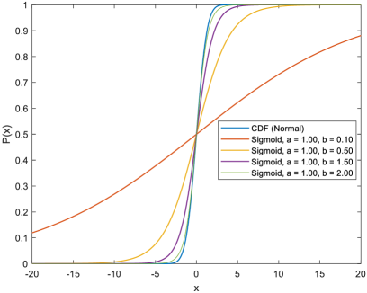
Figure 1: Different types of likelihood function.

The sigmoid likelihood function is inherently smooth and differentiable, thus is well-suited for optimization tasks. Compared to the CDF likelihood, the sigmoid function offers greater computational efficiency and seamless integration into neural networks for training purposes. By tuning the parameters of the sigmoid function, it can effectively model the impact of noise, thereby enhancing performance, particularly in low SNR conditions. Furthermore, the sigmoid likelihood function is highly versatile and can be readily extended to address more complex scenarios, such as non-Gaussian noise or colored noise, making it a robust choice for a wide range of applications.

Denote $\tilde{\mathbf{x}}=\frac{\mathbf{x}}{\sigma}$, and notice

$$P\left(\overline{\mathbf{y}}=1\right)=P\left(\mathbf{\mathcal{A}}\mathbf{x}+\mathbf{n}\geq 0\right)=P\left(\mathbf{\mathcal{A}}\tilde{\mathbf{x}}+\bm{\epsilon}\geq 0\right),$$ (29)

where $\bm{\epsilon}$ is the normalized noise term that follows a standard normal distribution. Similarly,

$$P\left(\overline{\mathbf{y}}=-1\right)=P\left(\mathbf{\mathcal{A}}\tilde{\mathbf{x}}+\bm{\epsilon}<0\right).$$ (30)

Thus, the posterior probability is constructed as:

$$p\left(\tilde{\mathbf{x}}\mid\overline{\mathbf{y}},\bm{\epsilon}\right)\propto p\left(\overline{\mathbf{y}}\mid\tilde{\mathbf{x}},\bm{\epsilon}\right)p\left(\tilde{\mathbf{x}}\right).$$ (31)

We can estimate $\tilde{\mathbf{x}}$ and $\bm{\epsilon}$ via the MAP approach as:

$$\left(\tilde{\mathbf{x}}^{\star},\bm{\epsilon}^{\star}\right)=\mathrm{arg}\max_{\tilde{\mathbf{x}},\bm{\epsilon}}p\left(\overline{\mathbf{y}}\mid\tilde{\mathbf{x}},\bm{\epsilon}\right)p\left(\tilde{\mathbf{x}}\right).$$ (32)

Following the same approach as in Section III-A, taking the negative logarithm of (32) yields the following non-convex objective function:

$$\mathcal{L}_{ongrid}^{\diamond}\left(\tilde{\mathbf{x}},\bm{\epsilon}\right)= -\ln{p\left(\overline{\mathbf{y}}\mid\tilde{\mathbf{x}},\bm{\epsilon}\right)}-\ln{p\left(\tilde{\mathbf{x}}\right)}$$

$$= \sum_{i=1}^{N}\ln{\left(1+\mathrm{a}\exp\left(-\mathrm{b}\overline{y}_{i}\left[\mathbf{a}_{i}^{\mathrm{T}}\tilde{\mathbf{x}}+\epsilon_{i}\right]\right)\right)}\$$

$$+\sum_{i=1}^{N}\ln{\left(1+\mathrm{a}\exp\left(-\mathrm{b}\overline{y}_{i}\left[\mathbf{a}_{i}^{\mathrm{T}}\tilde{\mathbf{x}}+\epsilon_{i}\right]\right)\right)}$$

$$+\sum_{i=1}^{N}\frac{\gamma\left|x_{i}\right|^{\alpha}}{\alpha}.$$ (33)

The same MM approach can be utilized to derive a majorizing function for $\mathcal{L}_{ongrid}^{\diamond}\left(\tilde{\mathbf{x}},\bm{\epsilon}\right)$. This leads to the derivation of a new closed-form update formula for each MM iteration.

III-C1 Majorizing Function for $\mathcal{L}^{\prime}\left(\tilde{\mathbf{x}},\bm{\epsilon}\right)$

Let $f\left(s\right)=\ln{\left(1+\mathrm{a}\exp\left(-\mathrm{b}s\right)\right)}$. With the second-order Taylor expansion of $f\left(s\right)$, we have:

$$f\left(s\right)\approx f\left(s^{k}\right)+f^{\prime}\left(s^{k}\right)\left(s-s^{k}\right)+\frac{f^{\prime\prime}\left(s^{k}\right)}{2}\left(s-s^{k}\right)^{2},$$ (34)

where $s^{k}$ is assumed to be available from the $k$-th iteration. The second-order derivative $f^{\prime\prime}(s^{k})$ is upper bounded by:

$$f^{\prime\prime}\left(s^{k}\right)=\frac{\mathrm{a}\mathrm{b}^{2}}{\exp(\mathrm{b}s^{k})+\mathrm{a}^{2}\exp(-\mathrm{b}s^{k})+2\mathrm{a}}\leq\frac{\mathrm{a}\mathrm{b}^{2}}{(\mathrm{a}+1)^{2}}.$$ (35)

Thus, $f\left(s\right)$ is upper bounded by:

$$f\left(s\right)\leq\frac{\mathrm{a}\mathrm{b}^{2}}{2(\mathrm{a}+1)^{2}}\left(s+\frac{(\mathrm{a}+1)^{2}}{\mathrm{a}\mathrm{b}^{2}}f^{\prime}(s^{k})-s^{k}\right)^{2}+\mathrm{const}.$$ (36)

By substituting (36) into (33) and applying smooth approximation on the second term in (33), we can obtain the majorizing function $\bar{\mathcal{L}}_{ongrid}^{\diamond}\left(\tilde{\mathbf{x}},\bm{\epsilon}\right)$ of $\mathcal{L}_{ongrid}^{\diamond}\left(\tilde{\mathbf{x}},\bm{\epsilon}\right)$:

$$\mathcal{L}_{ongrid}^{\diamond}\left(\tilde{\mathbf{x}},\bm{\epsilon}\right)\leq \bar{\mathcal{L}}_{ongrid}^{\diamond}\left(\tilde{\mathbf{x}},\bm{\epsilon}\right)$$

$$= \frac{\mathrm{a}\mathrm{b}^{2}}{2(\mathrm{a}+1)^{2}}\left\|\mathbf{\mathcal{A}}\tilde{\mathbf{x}}-\mathbf{\mathcal{A}}\tilde{\mathbf{x}}^{k}+\bm{\epsilon}-\bm{\epsilon}^{k}-g(\tilde{\mathbf{x}}^{k},\bm{\epsilon}^{k})\right\|^{2}$$

$$+\frac{\gamma}{\alpha}\sum_{i=1}^{N}\left(\left|\tilde{x}_{i}\right|^{2}+\eta\right)^{\frac{\alpha}{2}}+\mathrm{const},$$ (37)

where

$$g(\tilde{\mathbf{x}}^{k},\bm{\epsilon}^{k})= \frac{(\mathrm{a}+1)^{2}\Re({\overline{\mathbf{y}}})}{\mathrm{b}\exp\left(\mathrm{b}\Re\left({\overline{\mathbf{y}}}\right)\odot\Re\left(\mathbf{\mathcal{A}}\tilde{\mathbf{x}}^{k}+\bm{\epsilon}^{k}\right)\right)+\mathrm{a}\mathrm{b}}$$

$$+j\frac{(\mathrm{a}+1)^{2}\Im({\overline{\mathbf{y}}})}{\mathrm{b}\exp\left(\mathrm{b}\Im({\overline{\mathbf{y}}})\odot\Im\left(\mathbf{\mathcal{A}}\tilde{\mathbf{x}}^{k}+\bm{\epsilon}^{k}\right)\right)+\mathrm{a}\mathrm{b}}.$$ (38)

III-C2 Updating Formula

The alternative minimization procedure is utilized to update $\tilde{\mathbf{x}}$ and $\bm{\epsilon}$. Specifically, $\tilde{\mathbf{x}}$ and $\bm{\epsilon}$ are updated iteratively by solving the following subproblems:

$${\tilde{\mathbf{x}}^{k+1}} =\mathrm{arg}\min_{\tilde{\mathbf{x}}}\bar{\mathcal{L}}_{ongrid}^{\diamond}\left(\tilde{\mathbf{x}},\bm{\epsilon}^{k}\right),$$ (39)

$$\bm{\epsilon}^{k+1} =\mathrm{arg}\min_{\bm{\epsilon}}\bar{\mathcal{L}}_{ongrid}^{\diamond}\left(\tilde{\mathbf{x}}^{k+1},\bm{\epsilon}\right).$$ (40)

For subproblem (39), following the same approach as in (17) or (24), we derive the estimate of $\tilde{\mathbf{x}}$:

$$\tilde{\mathbf{x}}^{k+1}\!=\!\left[\mathbf{\mathcal{A}}^{\mathrm{H}}\mathbf{\mathcal{A}}+\frac{\gamma^{k}(\mathrm{a}+1)^{2}}{\mathrm{a}\mathrm{b}^{2}}\bm{\Lambda}(\tilde{\mathbf{x}}^{k})\right]^{-1}\!\!\mathbf{\mathcal{A}}^{\mathrm{H}}\left[\mathbf{\mathcal{A}}\tilde{\mathbf{x}}^{k}+g(\tilde{\mathbf{x}}^{k},\bm{\epsilon}^{k})\right],$$ (41)

where

$$\bm{\Lambda}\left(\tilde{\mathbf{x}}^{k}\right)=\mathrm{diag}\left(\left(\left|\tilde{x}_{1}^{k}\right|^{2}+\eta\right)^{\frac{\alpha}{2}-1},\cdots,\left(\left|\tilde{x}_{N}^{k}\right|^{2}+\eta\right)^{\frac{\alpha}{2}-1}\right).$$

We then alternatively update $\bm{\epsilon}^{k+1}$ as:

$$\bm{\epsilon}^{k+1}=\bm{\epsilon}^{k}-\mathbf{\mathcal{A}}\left[\tilde{\mathbf{x}}^{k+1}-\tilde{\mathbf{x}}^{k}\right]+g(\tilde{\mathbf{x}}^{k},\bm{\epsilon}^{k}).$$ (42)

The augmented framework, referred to as sparse Bayesian reweighted iterative X (SBRI-X) for one-bit on-grid DOA estimation, is summarized in Algorithm 3.

Algorithm 3 SBRI-X for One-Bit On-Grid DOA.

1:Input: $\overline{\mathbf{y}}$, $\mathbf{\mathcal{A}}$, $T_{\max}$, $\alpha$, $\mathrm{a}$, $\mathrm{b}$, $\eta$ $\gamma^{0}$, error bound $\epsilon_{0}$

2:Output: $\hat{\mathbf{x}}^{\star}$

3:Initialize $\hat{\mathbf{x}}^{0}=\frac{\mathcal{A}^{H}\overline{\mathbf{y}}}{\|\mathcal{A}^{H}\overline{\mathbf{y}}\|_{2}}$

4:for $k\leftarrow 1$ to $T_{\max}$ do

5:  Update $\tilde{\mathbf{x}}^{k}$ using the formula in (41)

6:  Update $\bm{\epsilon}^{k}$ using the formula in (42)

7:  Update $\gamma^{k}$ using the formula in (19)

8:  if ($\frac{\|\hat{\mathbf{x}}^{(k+1)}\!\!-\hat{\mathbf{x}}^{(k)}\|_{2}^{2}}{\|\hat{\mathbf{x}}^{(k)}\|_{2}^{2}}\!\leq\!\epsilon_{0}$ and $\frac{\|\bm{\epsilon}^{k+1}\!\!-\bm{\epsilon}^{k}\|_{2}^{2}}{\|\bm{\epsilon}^{k}\|_{2}^{2}}\!\leq\!\epsilon_{0})$ or $k\!\geq\!T_{\mathrm{max}}$ then

9:   break

10:  else

11:   $\hat{\mathbf{x}}^{k+1}\leftarrow\hat{\mathbf{x}}^{k}$

12:   $\bm{\epsilon}^{k+1}\leftarrow\bm{\epsilon}^{k}$

13:   $\gamma^{k+1}\leftarrow\gamma^{k}$

14:  end if

15:end for

16:return $\hat{\mathbf{x}}^{\star}\leftarrow\hat{\mathbf{x}}^{k}$

For an off-grid model, the main update steps in the augmented framework are similar to those in (24) and (25), as outlined below:

$$\tilde{\mathbf{x}}^{k+1}= \left[\mathbf{C}^{\mathrm{H}}(\bm{\beta}^{k})\mathbf{C}(\bm{\beta}^{k})+\frac{\gamma(\mathrm{a}+1)^{2}}{\mathrm{a}\mathrm{b}^{2}}\bm{\Lambda}^{-1}(\tilde{\mathbf{x}}^{k})\right]^{-1}$$

$$\cdot\mathbf{C}^{\mathrm{H}}(\bm{\beta}^{k})\left[\mathbf{C}(\bm{\beta}^{k})\tilde{\mathbf{x}}^{k}+g^{\dagger}(\tilde{\mathbf{x}}^{k},\bm{\epsilon}^{k},\bm{\beta}^{k})\right],$$ (43)

where

$$g^{\dagger}(\tilde{\mathbf{x}}^{k},\bm{\epsilon}^{k})= \frac{(\mathrm{a}+1)^{2}\Re({\overline{\mathbf{y}}})}{\mathrm{b}\exp\left(\mathrm{b}\Re({\overline{\mathbf{y}}})\odot\Re\left(\mathbf{C}(\bm{\beta}^{k})\tilde{\mathbf{x}}^{k}+\bm{\epsilon}^{k}\right)\right)+\mathrm{a}\mathrm{b}}$$

$$+j\frac{(\mathrm{a}+1)^{2}\Im({\overline{\mathbf{y}}})}{\mathrm{b}\exp\left(\mathrm{b}\Im({\overline{\mathbf{y}}})\odot\Im\left(\mathbf{C}(\bm{\beta}^{k})\tilde{\mathbf{x}}^{k}+\bm{\epsilon}^{k}\right)\right)+\mathrm{a}\mathrm{b}}.$$ (44)

The update for $\bm{\epsilon}$ is given by:

$$\bm{\epsilon}^{k+1}=\bm{\epsilon}^{k}-\mathbf{C}(\bm{\beta}^{k})\left(\tilde{\mathbf{x}}^{k+1}-\tilde{\mathbf{x}}^{k}\right)+g^{\dagger}(\tilde{\mathbf{x}}^{k},\bm{\epsilon}^{k},\bm{\beta}^{k}),$$ (45)

and the update for grid gaps $\bm{\beta}$ follows:

$$\bm{\beta}^{k+1} =\left[\Re\left((\mathcal{B}^{\mathrm{H}}\mathcal{B})^{*}(\tilde{\mathbf{x}}^{k+1}\!-\tilde{\mathbf{x}}^{k})(\tilde{\mathbf{x}}^{k+1}-\tilde{\mathbf{x}}^{k})^{\mathrm{H}}\right)\right]^{-1}$$

$$\cdot\Re\left(\mathrm{diag}(\tilde{\mathbf{x}}^{k+1}\!-\!\tilde{\mathbf{x}}^{k})^{*}\mathcal{B}^{\mathrm{H}}\!\left[g^{\dagger}(\tilde{\mathbf{x}}^{k},\bm{\epsilon}^{k},\bm{\beta}^{k})\!-\!\mathcal{A}(\tilde{\mathbf{x}}^{k+1}\!-\!\tilde{\mathbf{x}}^{k})\right]\right).$$ (46)

The constraint on the grid gaps, $\beta_{n}\in\left[-\frac{r}{2},\frac{r}{2}\right]$, is enforced to guarantee that:

$$\beta_{n}^{k+1}=\begin{cases}\beta_{n}^{k+1},&\text{if }\beta_{n}^{k+1}\in\left[-\frac{r}{2},\frac{r}{2}\right],\\ -\frac{r}{2},&\text{if }\beta_{n}^{k+1}<-\frac{r}{2},\\ \frac{r}{2},&\text{otherwise}.\end{cases}$$ (47)

The SBRI-X for one-bit off-grid DOA estimation is outlined in Algorithm 4.

Algorithm 4 SBRI-X for One-Bit Off-Grid DOA.

1:Input: $\overline{\mathbf{y}}$, $\mathbf{\mathcal{A}}$, $\mathbf{\mathcal{B}}$, $T_{\max}$, $\alpha$, $\mathrm{a}$, $\mathrm{b}$, $\eta$, $\gamma^{0}$, error bound $\epsilon_{0}$

2:Output: $\hat{\mathbf{x}}^{\star}$

3:Initialize $\tilde{\mathbf{x}}^{0}=\frac{\mathcal{A}^{H}\overline{\mathbf{y}}}{\|\mathcal{A}^{H}\overline{\mathbf{y}}\|_{2}}$, $\bm{\beta}^{0}=\mathbf{0}$

4:for $k\leftarrow 1$ to $T_{\max}$ do

5:  Update $\tilde{\mathbf{x}}^{k}$ using the formula in (43)

6:  Update $\bm{\epsilon}^{k}$ using the formula in (45)

7:  Update $\bm{\beta}^{k}$ using the formulas in (46) and (47)

8:  Update $\lambda^{k}$ using the formula in (19)

9:  if ($\frac{\|\hat{\mathbf{x}}^{(k+1)}\!\!-\hat{\mathbf{x}}^{(k)}\|_{2}^{2}}{\|\hat{\mathbf{x}}^{(k)}\|_{2}^{2}}\!\leq\!\epsilon_{0}$ and $\frac{\|\bm{\epsilon}^{k+1}\!\!-\bm{\epsilon}^{k}\|_{2}^{2}}{\|\bm{\epsilon}^{k}\|_{2}^{2}}\!\leq\!\epsilon_{0}$) or $k\!\geq\!T_{\mathrm{max}}$ then

10:   break

11:  else

12:   $\tilde{\mathbf{x}}^{k+1}\leftarrow\tilde{\mathbf{x}}^{k}$

13:   $\bm{\epsilon}^{k+1}\leftarrow\bm{\epsilon}^{k}$

14:   $\bm{\beta}^{k+1}\leftarrow\bm{\beta}^{k}$

15:   $\gamma^{k+1}\leftarrow\gamma^{k}$

16:  end if

17:end for

18:return $\tilde{\mathbf{x}}^{\star}\leftarrow\hat{\mathbf{x}}^{k}$

IV Model-Based Neural Networks for One-Bit DOA Estimation

In this section, we design model-based neural networks to address both one-bit on-grid and off-grid DOA estimation tasks. Inspired by the algorithm unrolling paradigm [39], the iterative steps of the sparse Bayesian reweighted iterative algorithms are mapped to customized neural layers.

Figure 2: End-to-end architecture of the SBRI-Net for the on-grid model.

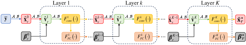
Figure 3: End-to-end architecture of the SBRI-Net for the off-grid model.

IV-A Inference Network Architecture

IV-A1 The SBRI-Net Framework

For on-grid estimation, the network structure corresponding to Algorithm 1 is illustrated in Figure 2. Next, we provide a detailed mathematical formulation of the network layers. Since the network parameters are defined using real values, we transform complex numbers into their real-valued counterparts. Specifically, the complex-valued measurement model (3) can be reformulated in the following real-valued form:

$$\overline{\mathbf{y}}_{r}=\mathrm{sign}\left(\mathbf{\mathcal{A}}_{r}\mathbf{x}_{r}+\mathbf{n}_{r}\right),$$ (48)

where subscript $r$ is used to emphasize real-valued valuables,

$$\overline{\mathbf{y}}_{r}= \begin{bmatrix}\Re(\overline{\mathbf{y}})\\ \Im(\overline{\mathbf{y}})\end{bmatrix}\in\mathbb{R}^{2M\times 1},$$ (49)

$$\mathbf{\mathcal{A}}_{r}= \begin{bmatrix}\Re({\mathbf{\mathcal{A}}})&-\Im({\mathbf{\mathcal{A}}})\\ \Im({\mathbf{\mathcal{A}}})&\Re({\mathbf{\mathcal{A}}})\end{bmatrix}\in\mathbb{R}^{2M\times 2N},$$ (50)

$$\mathbf{x}_{r}= \begin{bmatrix}\Re(\mathbf{x})\\ \Im(\mathbf{x})\end{bmatrix}\in\mathbb{R}^{2N\times 1},$$ (51)

$$\mathbf{n}_{r}= \begin{bmatrix}\Re(\mathbf{n})\\ \Im(\mathbf{n})\end{bmatrix}\in\mathbb{R}^{2M\times 1}.$$ (52)

The input to the network is the same as the initialization step in the algorithm framework but using real values $\hat{\mathbf{x}}_{r}^{0}=\mathcal{A}_{r}^{T}\overline{\mathbf{y}}_{r}$. For the $k$-th layer of the network, the input is $\hat{\mathbf{x}}_{r}^{k-1}$. The computation of $\hat{\mathbf{v}}_{r}^{k}$ is given by:

$$\hat{\mathbf{v}}_{r}^{k}=\overline{\mathbf{y}}_{r}\odot\left(\mathbf{d}_{r}^{k}-\mathrm{I}^{\prime}(\mathbf{d}_{r}^{k})\right)$$ (53)

with $\mathbf{d}_{r}^{k}=\overline{\mathbf{y}}_{r}\odot(\mathbf{\mathcal{A}}_{r}\mathbf{x}_{r}^{k-1})$. Instead of using the update formula in (17), the CNN structures are utilized to avoid matrix inversion operations. Consequently, $\mathbf{x}$ is updated as:

$$\hat{\mathbf{x}}_{r}^{k}=F_{conv}^{k}\left(\mathbf{\mathcal{A}}_{r}^{\mathrm{T}}\hat{\mathbf{v}}_{r}^{k-1};\mathbf{W}_{conv}^{k},\mathbf{b}_{conv}^{k}\right),$$ (54)

where $F_{conv}^{k}$ represents the CNN structure in the $k$-th layer, and $\mathbf{W}_{conv}^{k}$ and $\mathbf{b}_{conv}^{k}$ denote its corresponding weights and biases, respectively. Assuming that the CNN structure consists of $J$ convolutional layers, the total number of convolutional layers is $KJ$.

Following the same design paradigm, we construct a similar network architecture for off-grid DOA estimation, as illustrated in Figure 3. The network initialization follows the same step as outlined in line 3 of Algorithm 2. The update for $\hat{\mathbf{v}}^{k}$ is computed as:

$$\hat{\mathbf{v}}_{r}^{k}=\overline{\mathbf{y}}_{r}\odot\left(\tilde{\mathbf{d}}_{r}^{k-1}-\mathrm{I}^{\prime}(\tilde{\mathbf{d}}_{r}^{k-1})\right),$$ (55)

where

$$\tilde{\mathbf{d}}_{r}^{k-1}=\overline{\mathbf{y}}_{r}\odot\left(\left[\mathbf{\mathcal{A}}_{r}+\mathbf{\mathcal{B}}_{r}\mathrm{diag}(\bm{\beta}_{r}^{k-1})\right]\hat{\mathbf{x}}_{r}^{k-1}\right).$$ (56)

The signal coefficients $\hat{\mathbf{x}}_{r}^{k}$ and grid gaps $\bm{\beta}_{r}^{k}$ are updated as:

$$\hat{\mathbf{x}}_{r}^{k} =F_{conv}^{k}\left(\left[\mathbf{\mathcal{A}}_{r}+\mathbf{\mathcal{B}}_{r}\mathrm{diag}(\bm{\beta}_{r}^{k-1})\right]^{\mathrm{T}}\hat{\mathbf{v}}_{r}^{k};\mathbf{W}_{k},\mathbf{b}_{k}\right),$$ (57)

$$\bm{\beta}_{r}^{k} =F_{FC}^{k}\left(\hat{\mathbf{x}}_{r}^{k};\mathbf{W}_{FC}^{k},\mathbf{b}_{FC}^{k}\right),$$ (58)

where $\mathbf{W}_{FC}^{k}$ and $\mathbf{b}_{FC}^{k}$ denote the weights and bias, respectively, for the $k$-th fully connected layer. Instead of updating the grid gaps as described in line 6 of Algorithm 2, we utilize fully connected layers to produce the grid gap estimates for the next layer.

IV-A2 The SBRI-X-Net Framework

The end-to-end structure of the augmented network is shown in Figure 4. Specifically, the initialization step follows the same as that in the vanilla network. For the $k$-th layer in the network, $\hat{\mathbf{u}}_{r}$ is updated as:

$$\hat{\mathbf{u}}_{r}^{k}=\mathbf{\mathcal{A}}_{r}\hat{\mathbf{x}}_{r}^{k-1}+g_{r}(\hat{\mathbf{x}}_{r}^{k-1},\hat{\bm{\epsilon}}_{r}^{k-1}),$$ (59)

where

$$g_{r}(\hat{\mathbf{x}}_{r}^{k-1},\hat{\bm{\epsilon}}_{r}^{k-1})=\frac{(\mathrm{a}_{k}+1)^{2}\overline{\mathbf{y}}_{r}}{\mathrm{b}_{k}\exp\left(\mathrm{b}_{k}\overline{\mathbf{y}}_{r}\odot\left[\mathbf{\mathcal{A}}\hat{\mathbf{x}}_{r}^{k-1}+\hat{\bm{\epsilon}}_{r}^{k-1}\right]\right)+\mathrm{a}_{k}\mathrm{b}_{k}}.$$ (60)

Noted that $\mathrm{a}_{k}$ and $\mathrm{b}_{k}$ are both learnable parameters during the end-to-end training. The updates for $\hat{\mathbf{x}}^{k}$ and $\hat{\bm{\epsilon}}_{r}^{k}$ are given by:

$$\hat{\mathbf{x}}_{r}^{k}= F_{conv}^{k}\left(\mathbf{\mathcal{A}}_{r}^{\mathrm{T}}\hat{\mathbf{u}}_{r}^{k};\mathbf{W}_{conv}^{k},\mathbf{b}_{conv}^{k}\right),$$ (61)

$$\hat{\bm{\epsilon}}_{r}^{k}= \bm{\epsilon}^{k-1}-\mathbf{\mathcal{A}}_{r}\left[\hat{\mathbf{x}}_{r}^{k}-\hat{\mathbf{x}}_{r}^{k-1}\right]+g_{r}(\hat{\mathbf{x}}_{r}^{k-1},\hat{\bm{\epsilon}}_{r}^{k-1}).$$ (62)

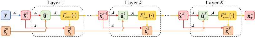
Figure 4: End-to-end architecture of the SBRI-X-Net for the on-grid model.

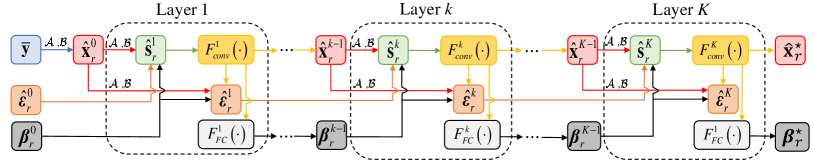
Figure 5: End-to-end architecture of the SBRI-X-Net for the off-grid model.

Similarly, the end-to-end architecture of the augmented network for the off-grid model is illustrated in Figure 5. In the $k$-th layer, the computation of $\hat{\mathbf{s}}^{k}$ is formulated as:

$$\hat{\mathbf{s}}^{k}=\left[\mathbf{\mathcal{A}}_{r}+\mathbf{\mathcal{B}}_{r}\mathrm{diag}(\bm{\beta}_{r}^{k-1})\right]\hat{\mathbf{x}}_{r}^{k-1}+g_{r}^{\dagger}(\hat{\mathbf{x}}_{r}^{k-1},\hat{\bm{\epsilon}}_{r}^{k-1},\bm{\beta}_{r}^{k-1}).$$ (63)

Finally, $\hat{\mathbf{x}}_{r}^{k}$, $\hat{\bm{\epsilon}}_{r}$ and the grid gaps $\bm{\beta}_{r}^{k}$ are updated as:

$$\hat{\mathbf{x}}_{r}^{k}= F_{conv}^{k}\left(\left[\mathbf{\mathcal{A}}_{r}+\mathbf{\mathcal{B}}_{r}\mathrm{diag}(\bm{\beta}_{r}^{k-1})\right]^{\mathrm{T}}\hat{\mathbf{s}}_{r}^{k-1};\mathbf{W}_{k},\mathbf{b}_{k}\right),$$ (64)

$$\hat{\bm{\epsilon}}_{r}^{k}= \bm{\epsilon}^{k-1}-\left[\mathbf{\mathcal{A}}_{r}+\mathbf{\mathcal{B}}_{r}\mathrm{diag}(\bm{\beta}_{r}^{k-1})\right]\left[\hat{\mathbf{x}}_{r}^{k}-\hat{\mathbf{x}}_{r}^{k-1}\right]$$

$$+g_{r}^{\dagger}(\hat{\mathbf{x}}_{r}^{k-1},\hat{\bm{\epsilon}}_{r}^{k-1},\hat{\bm{\beta}}_{r}^{k-1}),$$ (65)

$$\bm{\beta}_{r}^{k}= F_{FC}^{k}\left(\hat{\mathbf{x}}_{r}^{k-1};\mathbf{W}_{FC}^{k},\mathbf{b}_{FC}^{k}\right).$$ (66)

IV-B Data Generation and Labeling

We generate training datasets for on-grid and off-grid DOA estimation tasks, respectively using two SLA configurations with half-wavelength element spacing: an 18-element array at $\frac{\lambda}{2}[0,1,2,3,4,7,8,9,10,11,12,13,14,15,16,17,18,19]$ and a 10-element array at $\frac{\lambda}{2}[0,3,4,5,6,7,11,16,18,19]$. The number of signals is set to 2, and the array field of view (FOV) is defined as $[-60^{\circ},60^{\circ}]$. For on-grid training data generation, the target DOAs are randomly sampled as integer degrees within the FOV. For off-grid training data generation, the angular space is discretized into uniform grids with a fixed grid size of $2^{\circ}$. The off-grid gaps corresponding to the signals are randomly generated following a uniform distribution $U\left(-1^{\circ},1^{\circ}\right)$. Reflection coefficients of the two signals are generated as random complex numbers, with their real and imaginary parts uniformly distributed in $U\left(0.5,1\right)$. Denoting the ground truth of the $n$-th DOA as set ${\mathbb{G}}_{n}$, the signals are labeled according to

$$\mathbf{s}_{n}^{\star}=\begin{cases}|s_{k}|,&\text{if }\theta_{k}\in\mathbb{G}_{n},\\ 0,&\text{otherwise,}\end{cases}$$ (67)

and off-grid gaps are labeled as:

$$\beta_{n}^{\star}=\begin{cases}|\beta_{k}|,&\text{if }\theta_{k}\in\mathbb{G}_{n},\\ 0,&\text{otherwise.}\end{cases}$$ (68)

We randomly generate $1,000,000$ samples across input SNR levels ranging between $0$ dB and $30$ dB in $5$ dB increments. $90\%$ of the dataset is used for training and the remaining $10\%$ is used for validation.

IV-C Loss Functions

The loss function used in the first stage is the binary cross-entropy (BCE) loss, defined as:

$$\mathcal{L}_{1}(\hat{\mathbf{x}},\mathbf{s}^{\star})=-\frac{1}{N}\sum_{i=1}^{N}\left[s_{i}^{\star}\cdot\mathrm{log}\hat{x}_{i}+(1-s_{i}^{\star})\cdot\mathrm{log}(1-\hat{x}_{i})\right].$$ (69)

In the second stage, we apply a combination of the mean squared error (MSE) loss and the BCE loss, and the total loss function is defined as:

$$\mathcal{L}_{2}(\hat{\mathbf{x}},\mathbf{s}^{\star};{\bm{\beta}},\bm{\beta}^{\star})=\mathcal{L}_{1}(\hat{\mathbf{x}},\mathbf{s}^{\star})+\frac{1}{N}\sum_{i=1}^{N}\left({\beta}_{i}-\beta_{i}^{\star}\right)^{2}.$$ (70)

IV-D Network Training

Our training methodology differs between the on-grid and off-grid models. For the on-grid model, we implement end-to-end training with $100$ epochs. In contrast, the off-grid model undergoes a two-stage training process with totaling $200$ epochs. In the first stage, only the signal coefficient update layers are trained using the first $100$ epochs, while the off-grid gap estimation layers remain frozen. This isolates the learning of signal coefficients, ensuring robust initial representations without off-grid interference. In the second stage, all layers are unfrozen and trained end-to-end using the left $100$ epochs, allowing the model to jointly optimize both signal coefficient updates and off-grid gap estimations. Both models use a batch size of $64$ and the Adam optimizer with a learning rate of $10^{-3}$. Training was conducted on a workstation with an Intel Core i9-9820X CPU and dual NVIDIA RTX 2080 GPUs.

V Numerical Results

This section presents a comprehensive performance evaluation of SBRI, SBRI-X, SBRI-Net, and SBRI-X-Net. In particular, we consider sparse target signals across various SLA configurations under different SNR conditions.

To analyze the performance of the proposed on-grid and off-grid algorithm frameworks, we use root mean square error (RMSE) and hit rate as the evaluation metrics. The RMSE is computed as $\mathrm{RMSE}=\sqrt{\frac{1}{N_{s}{K}}\sum_{t=1}^{N_{s}}||\hat{\bm{\theta}}_{t}-\bm{\theta}^{\star}||_{2}^{2}}$, where $\hat{\bm{\theta}}_{t}$ represents the estimated DOA vector in the $t$-th test round, $K$ is the number of signals, and $N_{s}$ is the number of successful tests. The hit rate is defined as $\mathrm{Hit\ rate}={N_{s}}/{N_{t}}$, where $N_{t}$ is the total number of simulation trails. A DOA estimate is considered successful if the absolute errors of all estimated angles remain within a threshold of $2^{\circ}$; otherwise, it is regarded as a failure.

V-A On-Grid DOA Estimation

We conducted $1,000$ simulation trials using an 18-element SLA to compare the average RMSE and hit rate of the proposed algorithm against the 1-bit SLIM method [26]. Figure 6(a) presents the estimation RMSEs of the proposed 1-bit SBRI and 1-bit SBRI-X, alongside 1-bit SLIM, across different input SNR levels. Figure 6 (b) illustrates the estimation hit rate for these methods. The test scenario consists of two fixed targets located at $\left[-30^{\circ},30^{\circ}\right]$. The proposed 1-bit SBRI-X achieves the lowest RMSE across all SNR levels, outperforming both 1-bit SLIM and 1-bit SBRI. Additionally, it demonstrates the highest estimation accuracy and highest hit rate in low input SNR conditions between 0 dB and 15 dB. These results highlight the performance gains of 1-bit SBRI-X over 1-bit SBRI and validate that the chosen sigmoid likelihood function contributes significantly to performance gains, particularly in low SNR conditions.

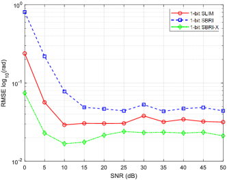
(a) RMSE vs. input SNR

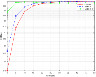
(b) Hit rate vs. input SNR

Figure 6: Performance comparison for on-grid DOA estimation using $18$-element SLA.

We further investigate the impact of parameter selection on the performance of the proposed 1-bit SBRI-X algorithm. As shown in Figure 1, parameter $\mathrm{b}$ controls the slopes of the likelihood functions. Figure 7 presents the estimation curves of 1-bit SBRI-X under different $\mathrm{b}$ settings. It can be observed that reducing $\mathrm{b}$ results in lower RMSEs across various SNR levels and a higher hit rate, indicating that smaller slopes of the likelihood function enhance the performance. It is also clear from Figure 7(a) that the RMSE initially decreases and then increases as the input SNR increases. This trend can be attributed to the influence of noise and quantization error at different SNR levels. In low SNR conditions, noise is the dominant factor affecting estimation accuracy, whereas in high SNR conditions, the impact of noise diminishes, and quantization error becomes the dominant factor. As shown in the results of Figure 8, the estimation errors decrease as the SNR increases and eventually converge. Additionally, Figure 8 presents the convergence curves for different choices of $\mathrm{b}$. It can be observed that smaller values of $\mathrm{b}$ (e.g., $\mathrm{b}=0.1$ or $\mathrm{b}=0.5$) result in a faster convergence rate, reaching smaller approximation error within approximately $10$ iterations.

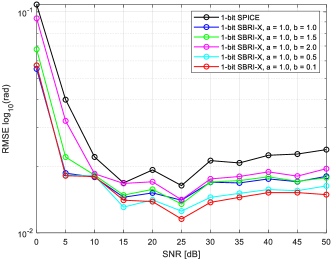
(a) RMSE vs. input SNR

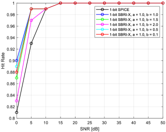
(b) Hit rate vs. input SNR

Figure 7: Effects of parameter selection on the performance of the proposed augmented algorithm framework for on-grid DOA estimation with an 18-element SLA.

To further evaluate the performance of the proposed SBRI-Net and SBRI-X-Net (illustrated in Figures 2 and 3), we conducted $5,000$ random trials using an 18-element SLA. These trials focused on a scenario with two fixed on-grid targets located at $\left[-10^{\circ},20^{\circ}\right]$ under varying SNR levels. The results were compared against optimization-based estimators, including 1-bit SPICE [26], 1-bit LIKES [26], and 1-bit SLIM [26]. As shown in Figures 9(a) and 9(b), SBRI-X-Net achieves comparable RMSE to SBRI-X at SNRs from $0$ dB to $15$ dB, and slightly lower RMSE at $20$ dB to $50$ dB. It also maintains a comparable hit rate across various SNR conditions, including those ranging from 35 dB to 50 dB, which were not part of the training scenarios. This demonstrates better overall performance and a certain level of generalization ability in high SNR conditions. A similar trend is observed for SBRI-Net, further demonstrating the effectiveness of the proposed model-based networks.

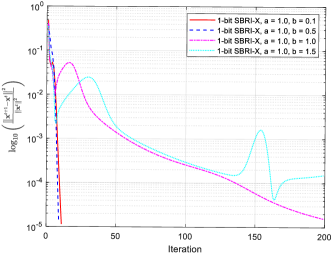
Figure 8: Convergence curves of 1-bit SBRI-X.

(a) RMSE vs. input SNR

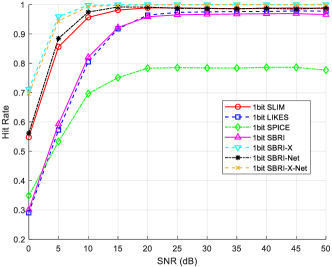
(b) Hit rate vs. input SNR

Figure 9: The performance of the proposed augmented algorithms and networks for on-grid DOA estimation with an 18-element SLA.

V-B Off-Grid DOA Estimation

We first conducted $5,000$ simulation trials on two fixed off-grid targets at $\left[-10.28^{\circ},20.56^{\circ}\right]$, using the 18-element SLA described in Section IV-B. The proposed algorithms and networks were evaluated against several benchmarks, including the pure data-driven CNN-DNN-based method proposed in [51], and other algorithms such as OGIR [35], 1-bit SLIM, 1-bit LIKES and 1-bit SPICE [26]. As shown in Figure 10(a), the off-grid methods consistently outperform on-grid algorithms. Among off-grid approaches, SBRI-X-Net achieved the lowest RMSE, while SBRI-Net performed on par with OGIR. Furthermore, the proposed model-based SBRI-X-Net and SBRI-Net exhibit superior performance over the pure data-driven CNN-DNN approach. From Figure 10(b), the proposed model-based approach achieves the highest hit rate across various SNR conditions, confirming the superior estimation performance of the proposed methods.

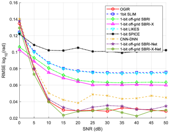
(a) RMSE vs. input SNR

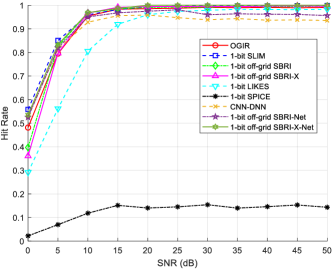
(b) Hit rate vs. input SNR

Figure 10: Performance comparison of SBRI-Net for off-grid DOA estimation using an $18$-element SLA.

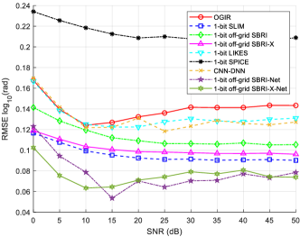
(a) RMSE vs. input SNR

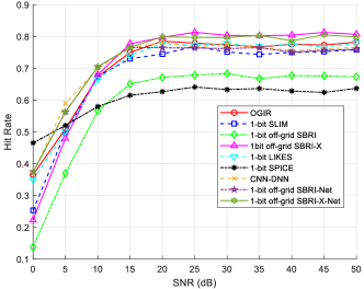
(b) Hit rate vs. input SNR

Figure 11: Performance comparison of SBRI-Net for off-grid DOA estimation using an $10$-element SLA.

In Figure 11, we further compare the performance of the proposed networks using the 10-element SLA described in Section IV-B. It can be observed that all methods experience performance degradation on the sparser 10-element SLA compared to their results with the 18-element SLA. However, the proposed model-based algorithms still outperform the other comparison algorithms, demonstrating their robustness for SLA configurations.

VI Conclusions

In this paper, we addressed the challenge problem of DOA estimation of off-grid signals using only a single snapshot of one-bit quantized data via a learning-based framework that synergizes model-driven sparse recovery with data-driven optimization. By reformulating DOA estimation under a MAP approach with a Laplacian-type sparsity prior, we unify on-grid and off-grid recovery while integrating a computationally efficient first-order grid approximation for practical one-bit systems with sparse arrays. The proposed SBRI and SBRI-X algorithms outperform existing model-based one-bit DOA methods in estimation accuracy across various SNR conditions and SLA configurations. Further, their neural network counterparts, SBRI-Net and SBRI-X-Net, achieve faster convergence by unrolling iterative optimization into interpretable deep neural layers, balancing computational efficiency with theoretical guarantees. The simulation results validate the superiority over existing methods in resolution threshold and hardware efficiency. This work advances scalable, high-resolution DOA estimation for next-generation sensing applications exploiting sparse arrays.

The derivations of the updating steps in Equations (24) and (25) are as follows. First, we compute the first-order derivative of the objective function in Equation (39) with respect to $\hat{\mathbf{x}}$:

$$\frac{\partial{\mathcal{L}}\left(\hat{\mathbf{x}},\bm{\beta}^{k}\right)}{\partial\hat{\mathbf{x}}}= \mathbf{C}^{\mathrm{H}}(\bm{\beta}^{k})\left[\mathbf{C}(\bm{\beta}^{k})\hat{\mathbf{x}}-\mathbf{w}^{k}\right]$$

$$+\gamma^{k}\sum_{i=1}^{N}\hat{x}_{i}\left(\left|\hat{x}_{i}\right|^{2}+\eta\right)^{\frac{\alpha}{2}-1}.$$ (71)

Setting the derivative to zero, we obtain:

$$\left[\mathbf{C}^{\mathrm{H}}(\bm{\beta}^{k})\mathbf{C}(\bm{\beta}^{k})+\gamma^{k}\bm{\Lambda}(\hat{\mathbf{x}})\right]\hat{\mathbf{x}}=\mathbf{C}^{\mathrm{H}}(\bm{\beta}^{k})\mathbf{w}^{k}.$$ (72)

Since $\bm{\Lambda}(\hat{\mathbf{x}})$ is a nonlinear function of $\hat{\mathbf{x}}$, Equation (72) is inherently nonlinear, making it challenging to solve directly. However, an iterative approximation method can be utilized to efficiently estimate its solution. In this approach, at each iteration, Equation (72) is approximated as a following linear problem:

$$\left[\mathbf{C}^{\mathrm{H}}(\bm{\beta}^{k})\mathbf{C}(\bm{\beta}^{k})+\gamma^{k}\bm{\Lambda}(\hat{\mathbf{x}}^{k})\right]\hat{\mathbf{x}}=\mathbf{C}^{\mathrm{H}}(\bm{\beta}^{k})\mathbf{w}^{k}.$$ (73)

The solution of (73) is given as:

$$\hat{\mathbf{x}}^{k+1}=\left[\mathbf{C}^{\mathrm{H}}(\bm{\beta}^{k})\mathbf{C}(\bm{\beta}^{k})+\gamma^{k}\bm{\Lambda}(\hat{\mathbf{x}}^{k})\right]^{-1}\mathbf{C}^{\mathrm{H}}(\bm{\beta}^{k})\mathbf{w}^{k}.$$ (74)

With the estimate $\hat{\mathbf{x}}^{k+1}$ obtained from Equation (74), we can further estimate $\bm{\beta}^{k+1}$. Rearrange the objective function as:

$$\mathcal{L}\left(\hat{\mathbf{x}},\bm{\beta}^{k}\right)= \frac{1}{2}\bigg{(}\bm{\beta}^{\mathrm{T}}\mathrm{diag}(\hat{\mathbf{x}}^{k+1})^{*}\mathbf{\mathcal{B}}^{\mathrm{H}}\mathbf{\mathcal{B}}\mathrm{diag}(\hat{\mathbf{x}}^{k+1})\bm{\beta}$$

$$+\bm{\beta}^{\mathrm{T}}\mathrm{diag}(\hat{\mathbf{x}}^{k+1})^{*}\mathbf{\mathcal{B}}^{\mathrm{H}}\left[\mathbf{\mathcal{A}}\hat{\mathbf{x}}^{k+1}-\mathbf{w}^{k}\right]$$

$$+(\hat{\mathbf{x}}^{k+1})^{\mathrm{H}}\mathbf{\mathcal{A}}^{\mathrm{H}}-(\mathbf{w}^{k})^{\mathrm{H}}\mathbf{\mathcal{B}}\mathrm{diag}(\hat{\mathbf{x}}^{k+1})\bm{\beta}\bigg{)}+C^{\prime},$$ (75)

where $C^{\prime}$ represents the sum of all terms that are not related to $\bm{\beta}$. Taking the first-order derivative of (75) and setting it to zero, we have:

$$\Re\left((\mathcal{B}^{\mathrm{H}}\mathcal{B})^{*}\hat{\mathbf{x}}^{k+1}(\hat{\mathbf{x}}^{k+1})^{\mathrm{H}}\right)\bm{\beta}$$

$$= \Re\left(\mathrm{diag}(\hat{\mathbf{x}}^{k+1})^{*}\mathcal{B}^{\mathrm{H}}\left[\mathbf{w}^{k}-\mathcal{A}\hat{\mathbf{x}}^{k+1}\right]\right).$$ (76)

Thus, we have the estimate of $\bm{\beta}^{k+1}$, given as:

$$\bm{\beta}^{k+1}= \left[\Re\left((\mathcal{B}^{\mathrm{H}}\mathcal{B})^{*}\hat{\mathbf{x}}^{k+1}(\hat{\mathbf{x}}^{k+1})^{\mathrm{H}}\right)\right]^{-1}$$

$$\times\Re\left(\mathrm{diag}(\hat{\mathbf{x}}^{k+1})^{*}\mathcal{B}^{\mathrm{H}}\left[\mathbf{w}^{k}-\mathcal{A}\hat{\mathbf{x}}^{k+1}\right]\right).$$ (77)

References

- [1] Y. Hu, S. Sun, and Y. D. Zhang, “Enhancing off-grid one-bit DOA estimation with learning-based sparse Bayesian approach for non-uniform sparse array,” in Proc. 58th Annual Asilomar Conference on Signals, Systems, and Computers, Pacific Grove, CA, Oct. 27-30, 2024.
- [2] S. Sedighi, B. S. Mysore R, M. Soltanalian, and B. Ottersten, “On the performance of one-bit DoA estimation via sparse linear arrays,” IEEE Transactions on Signal Processing, vol. 69, pp. 6165–6182, 2021.
- [3] S. Sun, A. P. Petropulu, and H. V. Poor, “MIMO radar for advanced driver-assistance systems and autonomous driving: Advantages and challenges,” IEEE Signal Processing Magazine, vol. 37, no. 4, pp. 98–117, 2020.
- [4] S. Sun and Y. D. Zhang, “4D automotive radar sensing for autonomous vehicles: A sparsity-oriented approach,” IEEE Journal of Selected Topics in Signal Processing, vol. 15, no. 4, pp. 879–891, 2021.
- [5] J. Li and P. Stoica, “MIMO radar with colocated antennas,” IEEE Signal Processing Magazine, vol. 24, no. 5, pp. 106–114, 2007.
- [6] S. M. Patole, M. Torlak, D. Wang, and M. Ali, “Automotive radars: A review of signal processing techniques,” IEEE Signal Processing Magazine, vol. 34, no. 2, pp. 22–35, 2017.
- [7] R. Schmidt, “Multiple emitter location and signal parameter estimation,” IEEE Transactions on Antennas and Propagation, vol. 34, no. 3, pp. 276–280, 1986.
- [8] R. Roy and T. Kailath, “ESPRIT–Estimation of signal parameters via rotational invariance techniques,” IEEE Transactions on Acoustics, Speech, and Signal Processing, vol. 37, no. 7, pp. 984–995, 1989.
- [9] B. Liao, Z.-G. Zhang, and S.-C. Chan, “DOA estimation and tracking of ULAs with mutual coupling,” IEEE Transactions on Aerospace and Electronic Systems, vol. 48, no. 1, pp. 891–905, 2012.
- [10] A. Moffet, “Minimum-redundancy linear arrays,” IEEE Transactions on Antennas and Propagation, vol. 16, no. 2, pp. 172–175, 1968.
- [11] P. Pal and P. P. Vaidyanathan, “Nested arrays: A novel approach to array processing with enhanced degrees of freedom,” IEEE Transactions on Signal Processing, vol. 58, no. 8, pp. 4167–4181, 2010.
- [12] P. P. Vaidyanathan and P. Pal, “Sparse sensing with co-prime samplers and arrays,” IEEE Trans. on Signal Processing, vol. 59, no. 2, pp. 573–586, 2011.
- [13] S. Qin, Y. D. Zhang, and M. G. Amin, “Generalized coprime array configurations for direction-of-arrival estimation,” IEEE Trans. on Signal Processing, vol. 63, no. 6, pp. 1377–1390, 2015.
- [14] Z. Zheng, W.-Q. Wang, Y. Kong, and Y. D. Zhang, “MISC array: A new sparse array design achieving increased degrees of freedom and reduced mutual coupling effect,” IEEE Transactions on Signal Processing, vol. 67, no. 7, pp. 1728–1741, 2019.
- [15] M. Viberg, B. Ottersten, and T. Kailath, “Detection and estimation in sensor arrays using weighted subspace fitting,” IEEE Transactions on Signal Processing, vol. 39, no. 11, pp. 2436–2449, 1991.
- [16] C. Zhou, Y. Gu, X. Fan, Z. Shi, G. Mao, and Y. D. Zhang, “Direction-of-arrival estimation for coprime array via virtual array interpolation,” IEEE Trans. on Signal Processing, vol. 66, no. 22, pp. 5956–5971, 2018.
- [17] O. Bar-Shalom and A. Weiss, “DOA estimation using one-bit quantized measurements,” IEEE Transactions on Aerospace and Electronic Systems, vol. 38, no. 3, pp. 868–884, 2002.
- [18] M. Ding, I. Atzeni, A. Tolli, and A. L. Swindlehurst, “On optimal MMSE channel estimation for one-bit quantized MIMO systems,” IEEE Transactions on Signal Processing, pp. 1–16, 2025.
- [19] L. V. Nguyen, A. L. Swindlehurst, and D. H. N. Nguyen, “Linear and deep neural network-based receivers for massive MIMO systems with one-bit ADCs,” IEEE Transactions on Wireless Communications, vol. 20, no. 11, pp. 7333–7345, 2021.
- [20] M. Shao, W.-K. Ma, Q. Li, and A. L. Swindlehurst, “One-bit Sigma-Delta MIMO precoding,” IEEE Journal of Selected Topics in Signal Processing, vol. 13, no. 5, pp. 1046–1061, 2019.
- [21] M. Kahlert, L. Xu, T. Fei, M. Gardill, and S. Sun, “High-resolution DOA estimation using single-snapshot MUSIC for automotive radar with mixed-ADC allocations,” in 2024 IEEE 13rd Sensor Array and Multichannel Signal Processing Workshop (SAM), 2024, pp. 1–5.
- [22] A. Eamaz, F. Yeganegi, Y. Hu, S. Sun, and M. Soltanalian, “Automotive radar sensing with sparse linear arrays using one-bit Hankel matrix completion,” in 2024 IEEE Radar Conference (RadarConf24), 2024.
- [23] A. Eamaz, F. Yeganegi, Y. Hu, M. Soltanalian, and S. Sun, “Collaborative automotive radar sensing via mixed-precision distributed array completion,” in Proc. IEEE 50th Intl. Conf. on Acoustics, Speech, and Signal Processing (ICASSP), Hyderabad, India, April 6-11, 2025.
- [24] A. Ameri, A. Bose, J. Li, and M. Soltanalian, “One-bit radar processing with time-varying sampling thresholds,” IEEE Transactions on Signal Processing, vol. 67, no. 20, pp. 5297–5308, 2019.
- [25] B. Jin, J. Zhu, Q. Wu, Y. Zhang, and Z. Xu, “One-bit LFMCW radar: Spectrum analysis and target detection,” IEEE Transactions on Aerospace and Electronic Systems, vol. 56, no. 4, pp. 2732–2750, 2020.
- [26] X. Shang, J. Li, and P. Stoica, “Weighted SPICE algorithms for range-Doppler imaging using one-bit automotive radar,” IEEE Journal of Selected Topics in Signal Process., vol. 15, no. 4, pp. 1041–1054, 2021.
- [27] K. Yu, Y. D. Zhang, M. Bao, Y.-H. Hu, and Z. Wang, “DOA estimation from one-bit compressed array data via joint sparse representation,” IEEE Signal Processing Letters, vol. 23, no. 9, pp. 1279–1283, 2016.
- [28] X. Huang and B. Liao, “One-bit MUSIC,” IEEE Signal Processing Letters, vol. 26, no. 7, pp. 961–965, 2019.
- [29] D. Malioutov, M. Cetin, and A. Willsky, “A sparse signal reconstruction perspective for source localization with sensor arrays,” IEEE Transactions on Signal Processing, vol. 53, no. 8, pp. 3010–3022, 2005.
- [30] D. Donoho, “Compressed sensing,” IEEE Transactions on Information Theory, vol. 52, no. 4, pp. 1289–1306, 2006.
- [31] L. Jacques, J. N. Laska, P. T. Boufounos, and R. G. Baraniuk, “Robust 1-bit compressive sensing via binary stable embeddings of sparse vectors,” IEEE Trans. on Info. Theory, vol. 59, no. 4, pp. 2082–2102, 2013.
- [32] F. Li, J. Fang, H. Li, and L. Huang, “Robust one-bit Bayesian compressed sensing with sign-flip errors,” IEEE Signal Processing Letters, vol. 22, no. 7, pp. 857–861, 2015.
- [33] X. Meng and J. Zhu, “A generalized sparse Bayesian learning algorithm for 1-bit DOA estimation,” IEEE Communications Letters, vol. 22, no. 7, pp. 1414–1417, 2018.
- [34] C. Zhou, Z. Zhang, F. Liu, and B. Li, “Gridless compressive sensing method for line spectral estimation from 1-bit measurements,” Digital Signal Processing, vol. 60, pp. 152–162, 2017.
- [35] L. Feng, L. Huang, Q. Li, Z.-Q. He, and M. Chen, “An off-grid iterative reweighted approach to one-bit direction of arrival estimation,” IEEE Trans. on Vehicular Technology, vol. 72, no. 6, pp. 8134–8139, 2023.
- [36] J. Shen, F. Gini, M. S. Greco, and T. Zhou, “Off-grid DOA estimation using improved root sparse Bayesian learning for non-uniform linear arrays,” EURASIP Journal on Advances in Signal Processing, vol. 34, pp. 1–22, 2023.
- [37] G. K. Papageorgiou, M. Sellathurai, and Y. C. Eldar, “Deep networks for direction-of-arrival estimation in low SNR,” IEEE Transactions on Signal Processing, vol. 69, pp. 3714–3729, 2021.
- [38] N. Shlezinger, J. Whang, Y. C. Eldar, and A. G. Dimakis, “Model-based deep learning,” Proc. of the IEEE, vol. 111, no. 5, pp. 465–499, 2023.
- [39] V. Monga, Y. Li, and Y. C. Eldar, “Algorithm unrolling: Interpretable, efficient deep learning for signal and image processing,” IEEE Signal Processing Magazine, vol. 38, no. 2, pp. 18–44, 2021.
- [40] J. P. Merkofer, G. Revach, N. Shlezinger, T. Routtenberg, and R. J. G. van Sloun, “DA-MUSIC: Data-driven DoA estimation via deep augmented MUSIC algorithm,” IEEE Transactions on Vehicular Technology, vol. 73, no. 2, pp. 2771–2785, 2024.
- [41] R. Zheng, H. Liu, S. Sun, and J. Li, “Deep learning based computationally efficient unrolling IAA for direction-of-arrival estimation,” in European Signal Processing Conference (EUSIPCO), 2023.
- [42] R. Zheng, S. Sun, H. Liu, H. Chen, and J. Li, “Interpretable and efficient beamforming-based deep learning for single-snapshot DOA estimation,” IEEE Sensors Journal, vol. 24, no. 14, pp. 22 096–22 105, 2024.
- [43] R. Zheng, S. Sun, H. Liu, and Y. D. Zhang, “Advancing single-snapshot DOA estimation with Siamese neural networks for sparse linear arrays,” in IEEE International Conference on Acoustics, Speech, and Signal Processing (CIASSP), Hyderabad, India, April 6-11, 2025.
- [44] F. Yeganegi, A. Eamaz, T. Esmaeilbeig, and M. Soltanalian, “Deep learning-enabled one-bit DoA estimation,” arXiv preprint arXiv:2405.09712, 2024.
- [45] S. D. Babacan, R. Molina, and A. K. Katsaggelos, “Bayesian compressive sensing using Laplace priors,” IEEE Transactions on Image Processing, vol. 19, no. 1, pp. 53–63, 2010.
- [46] C. D. Gianelli, “One-bit compressive sampling with time-varying thresholds: The Cramér-Rao bound, maximum likelihood, and sparse estimation,” Ph.D. dissertation, University of Florida, 2019.
- [47] J. Ren, T. Zhang, J. Li, and P. Stoica, “Sinusoidal parameter estimation from signed measurements via majorization–minimization based RELAX,” IEEE Transactions on Signal Processing, vol. 67, no. 8, pp. 2173–2186, 2019.
- [48] Y. Sun, P. Babu, and D. P. Palomar, “Majorization-minimization algorithms in signal processing, communications, and machine learning,” IEEE Trans. on Signal Processing, vol. 65, no. 3, pp. 794–816, 2017.
- [49] I. Daubechies, R. DeVore, M. Fornasier, and C. S. Güntürk, “Iteratively reweighted least squares minimization for sparse recovery,” Communications on Pure and Applied Mathematics, vol. 63, no. 1, pp. 1–38, 2010.
- [50] Z. Yang, L. Xie, and C. Zhang, “Off-grid direction of arrival estimation using sparse Bayesian inference,” IEEE Transactions on Signal Processing, vol. 61, no. 1, pp. 38–43, 2012.
- [51] H. Chung, H. Seo, J. Joo, D. Lee, and S. Kim, “Off-grid DOA estimation via two-stage cascaded neural network,” Energies, vol. 14, no. 1, p. 228, 2021.