The mean value property (corrected version)111This is a corrected version of the paper ”The mean value property, Mathematical Intelligencer, 37(2015), 9–16.”. In the original paper an incorrect claim was stated about the connection of harmonic functions and minimal surfaces. In the present version that incorrect claim is eliminated and the relation in question is explained in more details in Section 8; the rest of the paper has not been changed.
“…what mathematics really consists of
is problems and solutions.” (Paul Halmos)
1 Some problem challenges
I like problems and completely agree with Paul Halmos that they are from the heart of mathematics ([7]). This one I heard when I was in high school.
Problem 1. Show that if numbers in between and are written into the squares of the integer lattice on the plane in such a way that each number is the average of the four neighboring numbers, then all the numbers must be the same.
Little did I know at that time that this problem has many things to do with random walks, the fundamental theorem of algebra, harmonic functions, the Dirichlet problem or with the shape of soap films.
A somewhat more difficult version is
Problem 2. Prove the same if the numbers are assumed only to be nonnegative.
Since 1949 every fall there is a unique mathematical contest in Hungary named after Miklós Schweitzer, a young mathematician perished during the siege of Budapest in 1945. It is for university students without age groups, and about 10-12 problems from various fields of mathematics are posted for 10 days during which the students can use any tools and literature they want.222The problems and solutions up to 1991 can be found in he two volumes [3] and [12] I proposed the following continuous variant of Problem 1 for the 1983 competition ([12, p. 34]).
Problem 3. Show that if a bounded continuous function on the plane has the property that its average over every circle of radius 1 equals its value at the center of the circle, then it is constant.
When “boundedness” is replaced here by “one-sided boundedness”, say positivity, the claim is still true, but the problem gets considerably tougher.
Problem 4. The boundedness in Problem 3 can be replaced by positivity.
We shall solve these problems and discuss their various connections. Although the first problem follows from the second one, we shall first solve Problem 1 because its solution will guide us in the solution of the stronger statement.
It will be clear that there is nothing special about the plane, the claims are true in any dimension.
-
•
If nonnegative numbers are written into every box of the integer lattice in in such a way that each number is the average of the neighboring numbers, then all the numbers are the same.
-
•
If a nonnegative continuous function in has the property that its average over every sphere of radius 1 equals its value at the center of the sphere, then it is constant.
It will also be clear that similar statements are true for other averages (like the one taken for the 9 touching squares instead of the 4 adjacent ones).
Label a square of the integer lattice by its lower-left vertex, and let be the number we write into the square. So Problem 1 asks for proving that if and for all we have
| (1) |
then all are the same. Note that some kind of limitations like boundedness or one-sided boundedness is needed, for, in general, functions with the property (1) need not be constant, consider e.g. . (1) is called the discrete mean value property for . First we discuss some of its consequences.
2 The maximum principle
Assume that satisfies (1) and it is nonnegative. Notice that if, say, takes the value 0 at an , then it must be zero everywhere. Indeed, then (1) gives that , , and all must be also 0, i.e. all the neighboring values must be zero. Repeating this we can get that all values of must be 0. The same argument works if takes its largest value at some point, so we have
Theorem 1
(Minimum/maximum principle) If a function with the discrete mean value property on the integer lattice attains somewhere its smallest/largest value, then it must be constant.
In particular, this implies a solution to Problem 1 if we assume that has a limit at infinity (i.e. for some as ). Unfortunately, in Problem 1 we do not know in advance that the function has a limit at infinity, so this is not a solution.
Call a subset of the squares of the integer lattice a region if every square in can be reached from every other square of by moving always inside to neighboring cells. The boundary of is the set of squares that are not in but which are neighboring to . See Figure 1 for a typical bounded region, where the boundary consists of the darker shaded squares.
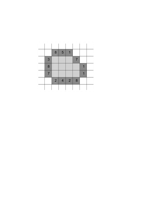
Suppose each boundary square contains a number like in Figure 1. Consider the number filling problem:
-
•
Can the squares of be filled in with numbers so that the discrete mean value property is true for all squares in ?
-
•
In how many ways can such a filling be done?
This problem is called the discrete Dirichlet problem, we shall see its connection with the classical Dirichlet problem later.
The unicity of the solution is easy to get. Indeed, it is clear that the maximum/minimum principle holds (with the proof given above) also on finite regions:
Theorem 2
(Maximum principle) Let be a function with the discrete mean value property on a finite region, and let be its largest value on . If attains somewhere in , then is the constant function.
This gives that if a function with the mean value property is zero on the boundary, then it must be zero everywhere, and from here the unicity of the solution to the discrete Dirichlet problem follows (just take the difference of two possible solutions).
Perhaps the most natural approach to the existence part of the number filling problem is to consider the numbers to be filled in as unknowns, to write up a system of equations for them which describes the discrete mean value property and the boundary properties of , and to solve that system. It can be readily shown that this linear system of equations is always solvable. But there is a better way to show existence that also works on unbounded regions.
3 Random walks
Consider a random walk on the squares of the integer lattice, which means that if at a moment we are in the lattice square , then we can move to any one of the neighboring squares , , or . Which one we choose depends on some random event, like throw two fair coins, and if the result is “Head-Head” then move to , if it is “Head-Tail” then move to , etc.
We would like to find the unique value of the square-filling problem at a point of the domain . Start a random walk from which stops when it hits the boundary of . Where it stops there is a prescribed number of the boundary, and since it is a random event which boundary point the walk hits first, that boundary number is also random. Now is the expected value of that boundary number. Indeed, from the walk moves to either of the four neighboring squares , , and with probability –, and then it continues as if it was started from there. So the just introduced expected value for will be the average of the expected values for , , and . Hence the mean value property is satisfied.
Unfortunately, it is not easy to calculate the hitting probabilities and the aforementioned expected value, but the connection with the discrete mean value property is notable. Furthermore, the order can be reversed, and this connection can be used to calculate certain probabilities. Consider the following question.
Problem 5. Two players, say H and T, where T is a dealer, repeatedly place 1–1 dollar on the table, flip a coin, and if it is Head, then H gets both notes, while if it is Tail, then T gets both of them. Suppose H starts with 30$, and wants to know her chance of having 100$ at some stage, when she quits the game.
Direct calculation of the probability of success for H is non-trivial and rather tedious. However, using the connection between random walks and functions with the discrete mean value property we can easily show that the answer is . To this end, let be the probability of success for H (i.e. reaching 100$) when she starts with dollars. After the first play H will have either or dollars with probability 1/2–1/2 (therefore, the fortune of H makes a random walk on the integer lattice), and from there the play goes on as if H started with resp. dollars. Therefore, satisfies the mean value property
| (2) |
What we have shown in dimension 2 remains true without any change in other dimensions, in particular, the discrete Dirichlet problem (2) has one and only one solution. But is clearly a solution to (2), so as was stated above. In general, if H starts with dollars and her goal is to reach dollars, then her chance of success is .
4 An iteration process
The two solutions to the discrete dirichlet problems discussed so far (solving linear systems or using random walks) are not too practical. Now we discuss a fast and simple method for approximating the solution.
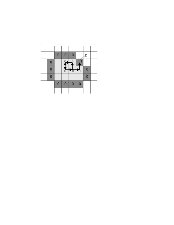
Let be a bounded region and let be a given function on the boundary . We need to find a function on which agrees with on the boundary and satisfies the discrete mean value property in . Define for any given on the function the following way: for in let
| (3) |
while on the boundary set . Note that we are looking for an that satisfies , so we are looking for a fixed point of the “operation” . Fixed points are often found by iteration: let be arbitrary and form . If this happens to converge, then the limit is a fixed point.
To start the iteration, let be the function which agrees with on the boundary and which is 0 on . Form , . It is a simple exercise to show that the iterates converge (necessarily to the solution of the discrete Dirichlet problem), and the speed of convergence is geometrically fast.
5 Solution to Problem 1
Let be a function on the lattice squares of the plain such that it has the discrete mean value property and its values lie in . We know from the maximum principle that if assumes somewhere an extremal (largest or smallest) value, then is constant.
The solution uses a similar idea, by considering the set of all such functions and considering
| (4) |
Since the translation of any by any vector is again in , and so is the rotation of by 90 degrees, it immediately follows that is actually the supremum of the differences of all possible values for neighboring squares and for . Thus, Problem 1 amounts the same as showing (necessarily ).
First of all, note that there is an for which
| (5) |
Indeed, by the definition of , for every there is an for which
By selecting repeatedly subsequences we get a subsequence for which the sequences converge for all . Now if
then clearly and (5) holds.
The function has again the discrete mean value property, and, according to what was said before, we have and . Thus, we get from the maximum principle that is constant, and the constant then must be . In particular, for all . Adding these for we obtain , which is possible for large only if , since . Hence, , as was claimed.
6 Sketch of the solution to Problem 2
Let now be a positive function on the lattice squares of the plain such that it has the discrete mean value property. Without loss of generality assume , and let be the family of all such ’s. Then the positivity of yields that , and repeating this argument it follows that for all and for all . Hence, the selection process in the preceding section can be carried out without any change in the family . Now consider
| (6) |
As before, turns out to be the supremum of the ratios for all neighboring squares and for all , therefore Problem 2 asks for showing that (clearly ).
Let be a function for which equality is assumed in (6) (the existence of follows from the selection process). Then
| (7) |
which can only be true if each one of the upper terms equals times the term below it (since each term in the numerator is at most times the term right below it). In particular, and . Repeat the previous argument to conclude that for all . Thus, there is some constant such that for all . Since and are also true, it follows as before that for all with some . Repeating again this argument we finally conclude that there are positive numbers such that is true for all .
Apply now the discrete mean value property:
| (8) |
Since , this implies , i.e. the concavity of the sequence . But a positive sequence on the integers can be concave only if it is constant. Thus, all the ’s are the same, and then (8) cannot be true if , hence as claimed.
7 The continuous mean value property and harmonic functions
Assume that is a domain (a connected open set) on the plane, and is a continuous real-valued function defined on . We say that has the mean value property in if for every circle which lies in together with its interior we have
| (9) |
where is the center of and denotes the length of . (9) means that the average of over the circle coincides with the function value at the center of .
Functions with this mean value property are called harmonic, and they play a fundamental role in mathematical analysis. For example, if is the real part of a complex differentiable (so called analytic) function, then is harmonic. The converse is also true in simply connected domains (domains without holes): if has the mean value property (harmonic), then it is the real part of a differentiable complex function. So there is an abundance of harmonic functions, e.g. the real part of any polynomial is harmonic, say
are all harmonic.
Although we shall not use it, we mention that the standard (but equivalent) definition of harmonicity is , where and denote the second partial derivatives of with respect to and . We shall stay with our geometric definition.
Simple consequence of the mean value property is the maximum principle:
Theorem 3
(Maximum principle) If a harmonic function on a domain attains somewhere its largest value, then it must be constant.
The reader can easily modify the argument given for Theorem 1 to verify this version.
A basic fact concerning harmonic functions is that a bounded harmonic function on the whole plane must be constant (Liouville’s theorem). I heard the following proof from Paul Halmos. Suppose satisfies (9) on the whole plane and it is bounded. Let be the disk of radius about some point . Since the integral over can be obtained by first integrating on circles of radius about and then integrating these integrals with respect to (from 0 to ), it easily follows that also has the area-mean value property:
| (10) |
If is another points, then the same formula holds for with replaced by . Now for very large the disks and are “almost the same” in the sense that outside their common part there are only two small regions in them the area of which is negligible compared to the area of the disks. So the averages of over and are practically the same (by the boundedness of ), and for we get that in the limit the averages, and hence also the function values at and are the same.
From here the fundamental theorem of algebra (“every polynomial has a zero on the complex plane”) is a standard consequence (if the polynomial did not vanish anywhere, then the real and imaginary parts of would be bounded harmonic functions on the plane, hence they would be constant, which is not the case).
Note that Problem 3 claims more than Liouville’s theorem, since in it the mean value property is requested only for circles with a fixed radius. In general, if we know the mean value property (9) for all circles of a fixed radius , then it does not follow that is harmonic. However, by a result of Jean Delsarte if (9) is true for all circles of radii equal to some or and does not lie in a finite exceptional set (consisting of the ratios of solutions of an equation involving a Bessel function), then must be harmonic. In this exceptional set is empty, and it is conjectured that it is empty in all , . See the most interesting paper [14], as well as the extended literature on Pompeiu’s problem in [15]–[16].
8 The Dirichlet problem and soap films
The Dirichlet problem in the continuous case is the following: suppose is a (bounded) domain with boundary , and there is a continuous function given on the boundary . Can this be (continuously) extended to to a harmonic function, i.e. can it be continued inside so that it has the mean value property there? Under some minimal regularity assumptions on the boundary this problem has always a unique solution .
The unicity follows from the maximum principle in the same fashion that was done in the discrete case. The existence requires additional assumptions, for example if is the punctured disk and we set for while , then there is no harmonic function in which continuously extends . But this example is pathological ( is an isolated point on the boundary), and it can be shown that in most cases the Dirichlet problem can be solved. Later we sketch how.
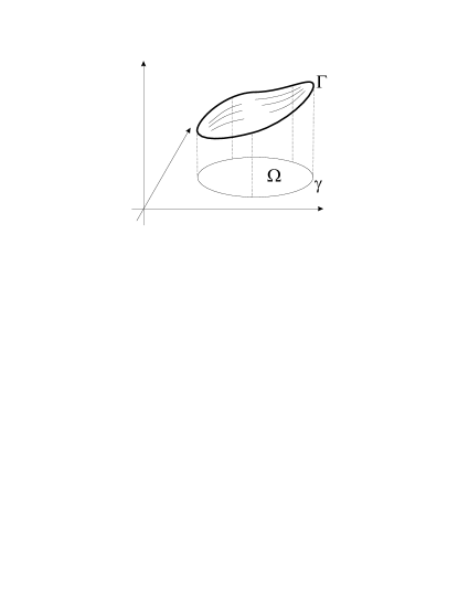
Suppose that the boundary of the domain is a simple closed curve with parametrization . Consider the given function on , and with its help lift up into 3 dimensions: is a 3 dimensional curve above . Now the points , , describe a surface that is attached to that space curve .
There are other surfaces attached to , among the most studied ones is the so called minimal surface with boundary . can be thought of as a wire, and stretch an elastic rubber sheet (or a soap film) over (see Figure 3). When in rest, the rubber sheet (soap film) gives a surface over the domain , which is the graph of a function . In general, is not the same as (the solution of the Dirichlet problem), i.e. is not harmonic (it can be characterized by a partial diffential equation). Nonetheless, (a so-called minimal surface – minimizing the area) can also be characterized via harmonic functions. To do that we need to introduced isothermal parametrizations.
Suppose we are given three continuous functions defined in a domain on the plane. Under some simple regularity conditions the points , , describe a surface in . In this case we say that , , gives in parametric form. If , , is a curve in , then
is a space curve that lies in . There are different ways to parametrize a surface , and a parametrization is called isothermal if it preserves the angle between curves, meaning that if and are (smooth) curves in that intersect each other, then the angle between and at their intersection point333The angle between two curves intersecting each other in a point is the angle that the tangents to the curves at form. is the same as the angle between the corresponding space curves and at their corresponding intersection point. Under some regularity conditions such an isothermal parametrization exists (at least locally, c.f. [9, p. 31].
Now it turns out (see e.g. [9, Lemma 4.2]) that a surface attached to with isothermal parametrization is the minimal surface if and only if all the parameter functions , , in its isothermal parametrization are harmonic funtions.
9 Discretization and Brownian motions
Is there a connection between the discrete and continuous Dirichlet problems discussed in Sections 2 and 8? There is indeed, and it is of practical importance.
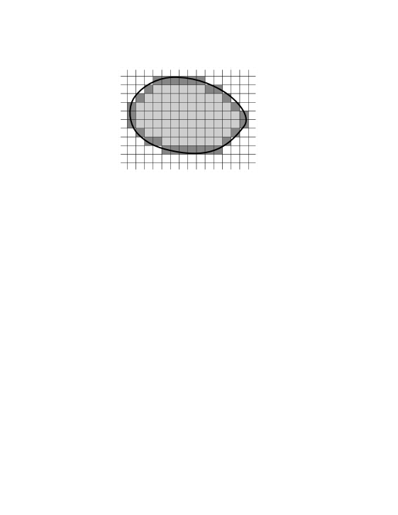
Let be a domain as in the preceding section, and let be a continuous function on the boundary of . Consider a square lattice on the plane with small mesh size, say consisting of size squares with small . Form a region (see Figure 4) on this lattice by considering those squares in the lattice which lie in (there may be a slight technical trouble that the union of these squares may not be connected, in that case let be the union of all squares that can be reached from a square containing a fixed point of ). We are going to consider the discrete Dirichlet problem on , the solution of which will be close to the solution of the original continuous Dirichlet problem. To this end define a boundary function on the boundary squares in our lattice: if is a boundary square, then must intersect the boundary , and if is any point, then set . Now solve this discrete Dirichlet problem on (with boundary numbers given by ) with the iteration technique of Section 4. Note that the iteration in Section 4 is computationally very simple and quite fast, since all one needs to do is to calculate averages of 4–4 numbers. Besides that, the convergence of the iterants to the solution is geometrically fast. Let be the solution, and we can imagine that gives us a function on the union of the squares belonging to : on every square the value of this is identically equal to the number . Now if is small, then this function will be close on to the solution of the continuous Dirichlet problem we are looking for.
There is yet another connection between the discrete and the continuous Dirichlet problems. We have seen in Section 3 that the discrete Dirichlet problem can be solved via random walks on the squares of the integer lattice. Now consider the just-introduced square lattice with small mesh size, and make a random walk on that lattice. If the mesh size is getting smaller then the lattice is getting denser (alternatively look at the square lattice from a far distance). To compensate for having more and more squares, speed up the random walk. If this speeding-up is done properly, then in the limit we get a random motion on the plane, the Brownian motion. In a Brownian motion a particle moves in such a way that it continuously and randomly changes its direction.
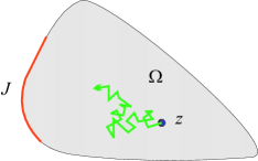
Let have smooth boundary, and let be an arc on that boundary, see Figure 5. Start a Brownian motion at a point , and stop it when it hits the boundary of , and let be the probability that it hits the boundary in a point of . This (which is called the harmonic measure of with respect to and ) has the mean value property. Indeed, consider a circle about the point that lies inside together with its interior. During the motion of the particle there is a fist time when the particle hits at a point . Then it continues as if it started in , and then the probability that it hits the boundary in a point of is . Because of the circular symmetry of , all play equal roles, and we can conclude (at least heuristically), that the hitting probability is the average of the hitting probabilities , , which is precisely the mean value property for . It is also clear that if is close to a point on the boundary of , then it is likely that the Brownian motion starting in will hit the boundary close to . Therefore, if (except when is one of the endpoints of ) the probability gets higher and higher, eventually converging to 1 as , while in the case when , the probability gets smaller and smaller, eventually converging to 0.
What we have shown is that is a harmonic function in which extends continuously to the boundary to 1 on the inner part of the arc and it extends continuously to 0 on the outer part of (therefore, at the endpoints cannot have a continuous extension). In other words, not worrying about continuity at the endpoints of the arc , we have solved the Dirichlet problem for the characteristic function
Now if is a continuous function on the boundary , then to there is arbitrarily close a function of the form with a finite sum, and then is a harmonic function in which is close to on the boundary. Using the maximum principle it follows that, as , the functions converge uniformly on to a function which has the mean value property in (since all had it) and which agrees with on . Therefore, this solves the Dirichlet problem.
We refer the interested reader to the book [11] for further reading concerning the mean value property and the Dirichlet problem. Robert Brown in “Brownian motion” was a Scottish botanist who, in 1827, observed in a microscope that pollen particles in suspension make an irregular, zigzag motion. The rigorous mathematical foundation of Brownian motion was made by Norbert Wiener in 1923 ([13]). The connection to the Dirichlet problem was first observed by Shizuo Kakutani [8]. This had a huge impact on further developments; there are many works that discuss the relation between random walks and problems (like the Dirichlet problem) in potential theory, see e.g. [10] or the very extensive [5].
10 Solution to Problem 4
In this proof we shall be brief, since some of the arguments have already been met before.
First of all, seemingly nothing prevents an as in Problem 4 behave wildly, and first we “tame” these functions. Let be the collection of all positive functions on the plane with the mean value property (9), and for some let be the collection of all the functions
| (11) |
for , where denotes the disk of radius about the point . If we can show that
is 1, then we are done. Indeed, then holds for all , and any with , which actually implies (just apply the inequality to and to ). Hence, since any two points on the plane can be connected by a polygonal line consisting of segments of length 1, every is constant, and then letting we get that every in is constant, as Problem 4 claims.
First we show that is finite. From the mean value property (9) we have for
| (12) | |||||
where is the disk of radius 2 about the origin, denotes area-integral and is a function on that is continuous and positive for . Thus, if is the ring and is the minimum of on that ring, then
Since for and for the ring contains the disk , it follows that
and upon taking the average for , the inequality follows. Hence, is finite.
From the finiteness of it follows that if is given and , then for all and all , where the constants depend only on . Let be the collection of all with . Then , and follows from (to be proven in a moment), where
Since is translation- and rotation-invariant, it is clear that
| (13) |
But the collection with consists of functions that are uniformly bounded and uniformly equicontinuous on all disks , , hence from every sequence of such functions one can select a subsequence that converges uniformly on all the disks , ,. Therefore, the supremum in (13) is attained, and there is an extremal function with . Suppose that holds for some (we have just seen that is such a value). From (12) it follows then that
and since here, by the definition of , for all , we can conclude that must be true for all . Thus, implies for all , and repeated application of this step gives that holds for all .
Now let be the collection of all that satisfies the just established functional equation , and let
Since is closed for translation and the operation (complex conjugation) taken in the argument, it follows that , and the reasoning we just gave for yields that there is an extremal function such that , and for this extremal function we have the functional equation for all . Thus, satisfies both equations , , from which it follows that if is the minimum of on the unit square, then at the integer lattice cell with lower left corner at .
Suppose now to the contrary that . Then the preceding estimate shows that as the real part of tends to infinity and the imaginary part stays nonnegative (then , ). Thus, if , then as the real part of tends to , and then
is a function with the mean value property which tends to infinity as (note that is positive, so , are larger than any of the terms on the right of their definitions). But this contradicts the maximum/minimum principle, and that contradiction proves that, indeed, .
11 The Krein-Milman theorem
Although all the proofs we gave were elementary, one should be aware of a general principle about extremal points that lies behind these problems. Recall that in a linear space a point is called an extremal point of a convex set if does not lie inside any segment joining two points of .
A linear topological space is called locally convex if the origin has a neighborhood basis consisting of convex sets. For example, -spaces are locally convex precisely for . Now a theorem of Mark Krein and David Milman says that if is a compact convex set in a locally compact topological space, then is the closure of the convex hull of its extremal points.
A point is an extremal point for a convex set precisely if it has the property that if lies in the convex hull of a set , then must be one of the points of . Now functions with a mean value property similar to those we considered in this article form a convex set (in the locally convex topological space of continuous or discrete functions), and the mean value property itself means that each such function lies in the convex hull of some of its translates. Therefore, such a function can be an extremal point for only if it agrees with all those translates, which means that it is constant. Now if the extremal points in are constants, then so are all functions in provided we can apply the Krein-Milman theorem. Hence, the crux of the matter is to prove that the additional boundedness or one-sided boundedness hypotheses set forth in our problems imply that is compact; then the Krein-Milman theorem finishes the job. In our proofs we faced the same problem: we needed the existence of extremal functions in (4), (6), (13), for which we needed to prove some kind of compactness.
In conclusion we mentioned that the problems that have been discussed in this paper are special cases of the Choquet-Deny convolution equation first discussed by Gustave Choquet and Jaques Deny in 1960, which has applications in probability theory and far reaching generalizations in various groups/spaces. See [1], [4] and the extended list of references in [2].
Acknowledgement. Part of this work was presented in 2011 at the Fazekas Mihály Gimnázium, Budapest, Hungary as a lecture for high school students. The author is thankful to András Hraskó and János Pataki for their comments regarding the presentation. The preparation of this paper was partially supported by NSF DMS-1265375. The author also thanks the anonymous referee for her/his helpful suggestions.
Special thanks go to José Gonzáles Llorente for pointing out the error in the original paper about the connection of harmonic functions and minimal surfaces.
References
- [1] G. Choquet and J. Deny, Sur l´équation de convolution , C.R. Acad. Sc. Paris, 250(1960), 779–801.
- [2] C. Chu and T. Hilberdink, The convolution equation of Choquet and Deny on nilpotent groups, Integr. Equat. Oper. Th., 26(1996), 1–13.
- [3] Contests in Higher Mathematics, 1949-1961, Akadémiai Kiadó, Budapest, 1968.
- [4] J. Deny, Sur l´équation de convolution , Sémin. Théor. Potentiel de M. Brelot, Paris 1960.
- [5] J. L. Doob, Classical potential theory and its probabilistic counterpart, Grundlehren der Mathematischen Wissenschaften, 262, Springer-Verlag, New York, 1984.
- [6] P. G. Doyle and J. L. Snell, Random walks and electric networks, Carus Mathematical Monographs, 22. Mathematical Association of America, Washington, DC, 1984.
- [7] P. Halmos, The heart of mathematics, Amer. Math. Monthly, 87(1980), 519–524.
- [8] S. Kakutani, Two-dimensional Brownian motion and harmonic functions, Proc. Imp. Acad., 20(1944), 706–714.
- [9] R. Osserman, A survey of minimal surfaces, Van Nostrand Reinhold Mathematical Studies, 25, New York, 1969.
- [10] S. C. Port and C. J. Stone, Brownian motion and classical potential theory, Probability and Mathematical Statistics, Academic Press, New York-London, 1978.
- [11] T. Ransford, Potential Theory in the Complex Plane, Cambridge University Press, Cambridge, 1995
- [12] G. Székely (editor), Contests in Higher Mathematics, Problem Books in Mathematics, Springer Verlag, New York, 1995.
- [13] N. Wiener, Differential space, Journal of Mathematical Physics, 2(1923) 131–174.
- [14] L. Zalcman, Offbeat integral geometry, Amer. Math. Monthly, 87(1980), 161–175.
- [15] L. Zalcman, A Bibliographic Survey of the Pompeiu Problem, Approximation by Solutions of Partial Differential Equations (Hanstholm, 1991), NATO Adv. Sci. Inst. Ser. C Math. Phys. Sci., 365, Kluwer Acad. Publ., Dordrecht, 1992, 185–194.
- [16] L. Zalcman, Supplementary bibliography to: ”A bibliographic survey of the Pompeiu problem” [in Approximation by solutions of partial differential equations (Hanstholm, 1991), 185–194, Kluwer Acad. Publ., Dordrecht, 1992], Radon transforms and tomography (South Hadley, MA, 2000), Contemp. Math., 278, Amer. Math. Soc., Providence, RI, 2001, 69–74.
Bolyai Institute
University of Szeged
Szeged
Aradi v. tere 1, 6720, Hungary
totik@mail.usf.edu