Simplified model of immunotherapy for glioblastoma multiforme: cancer stem cells hypothesis perspective

Wiktor Jochymczyk,  Urszula Foryś
(February 9, 2025)
Abstract

Despite ongoing efforts in cancer research, a fully effective treatment for glioblastoma multiforme (GBM) is still unknown. Since adoptive cell transfer immunotherapy is one of the potential cure candidates, efforts have been made to assess its effectiveness using mathematical modeling. In this paper, we consider a model of GBM immunotherapy proposed by Abernathy and Burke (2016), which also takes into account the dynamics of cancer stem cells, i.e., the type of cancer cells that are hypothesized to be largely responsible for cancer recurrence. We modify the initial ODE system by applying simplifying assumptions and analyze the existence and stability of steady states of the obtained simplified model depending on the treatment levels.

1 Introduction

Glioblastoma multiforme (GBM) accounts for 15.6%15.6\% of all and up to 45.2%45.2\% of malignant primary brain tumors [1]. Due to its sensitive location, high heterogeneity and strong suppression of the immune response, the therapy that allows for a complete cure is still unknown [2, 3]. Among patients diagnosed with GBM, the median survival time from diagnosis is 15 months and less than 5%5\% of patients survive 55 years from diagnosis [1, 4].

The commonly accepted treatment for GBM consists of tumor resection followed by radiotherapy combined with temozolomide chemotherapy [5]. Due to the low effectiveness of conventional therapy, research on alternative treatment methods is still ongoing. These include various types of immunotherapy, such as treatment with cancer vaccines, oncolytic viruses, immune checkpoint inhibitors, and adoptive cell transfer [6].

In [7], Kronik et al. presented a mathematical model for the treatment of GBM by adoptive transfer of cytotoxic T cells. That work was then continued by Kogan et al. in [8]. More precisely, in [8], the model proposed in [7] was first generalized by assuming certain properties of the functions that describe the processes considered in the original article and reflected in that article by specific functions. For this generalized model, Kogan et al. proved the boundedness of solutions and the dissipativity of the model. Since every dissipative system has a global attractor, steady states were studied as candidates for it. In the general case, the steady states established for the untreated system were considered. Then, for the system with treatment, conditions for tumor elimination were proposed. The final section was devoted to confronting analytical and numerical results with clinical data.

In [9], Abernathy and Burke built on previous results and modified the general model from [8] to include cancer stem cells (CSCs). The CSC hypothesis states that a special type of cancer cells with properties similar to healthy stem cells is largely responsible for the formation and development of cancer. These cells are thought to multiply much faster than normal cancer cells and then differentiate into other types of cancer cells. Theoretically, if even a small number of CSCs survive treatment, it could lead to relapse.

The GBM development and immunotherapy model considered in this article is based on the ODE system presented in [9]. First, we adopt the notation used in that article:

  • TT and SS will refer to the number of ordinary cancer cells and CSCs, respectively;

  • CC will be the number of cytotoxic T lymphocytes that fight the tumor;

  • xx, yy will refer to the amount of transforming growth factor beta (TGF-β\beta) and the amount of interferon gamma (IFN-γ\gamma) in the vicinity of the tumor, respectively;

  • uu and vv will be the average number of major histocompatibility complex molecules of class I and II (MHC class I and II) per tumor cell, respectively.

With the above notation, the model proposed in [9] has the following form:

T˙\displaystyle\dot{T} =α(T,S)+RT(T)TfT(x)gT(u)hT(T)CT,\displaystyle=\alpha(T,S)+R_{T}(T)T-f_{T}(x)g_{T}(u)h_{T}(T)CT, (\theparentequation.1)
S˙\displaystyle\dot{S} =RS(S)Sα(T,S)fS(x)gS(u)hS(S)CS,\displaystyle=R_{S}(S)S-\alpha(T,S)-f_{S}(x)g_{S}(u)h_{S}(S)CS, (\theparentequation.2)
C˙\displaystyle\dot{C} =fC((T+S)v)gC(x)μCC+N(t),\displaystyle=f_{C}((T+S)v)g_{C}(x)-\mu_{C}C+N(t), (\theparentequation.3)
x˙\displaystyle\dot{x} =fx(T,S)μxx,\displaystyle=f_{x}(T,S)-\mu_{x}x, (\theparentequation.4)
y˙\displaystyle\dot{y} =fy(C)μyy,\displaystyle=f_{y}(C)-\mu_{y}y, (\theparentequation.5)
u˙\displaystyle\dot{u} =fu(y)μuu,\displaystyle=f_{u}(y)-\mu_{u}u, (\theparentequation.6)
v˙\displaystyle\dot{v} =fv(x)gv(y)μvv.\displaystyle=f_{v}(x)g_{v}(y)-\mu_{v}v. (\theparentequation.7)

We will now present interpretations of the equations of System (1). Equation (\theparentequation.1) describes the change in the number of tumor cells over time. The function α\alpha is responsible for the process of stem cells differentiating into regular cancer cells, while the function RTR_{T} describes the growth of the tumor cell population per capita. The third term reflects the efficiency with which lymphocytes destroy cancer cells. The functions fTf_{T}, gTg_{T}, and hTh_{T} introduce a dependence of this process on the amount of TGF-β\beta in the vicinity of the tumor, the average number of MHC class I molecules per tumor cell and the size of the population of tumor cells, respectively.

Similarly, Equation (\theparentequation.2) describes the change in the CSC population over time. In this case, the function RSR_{S} describes the growth of the CSC population per capita, and the last term reflects the efficiency with which lymphocytes destroy CSCs, analogously to Eq. (\theparentequation.1). The change in the population of lymphocytes is in turn described by Eq. (\theparentequation.3). The functions fCf_{C}, gCg_{C} make this process dependent on the total number of MHC class II molecules on the surface of all tumor cells and the amount of TGF-β\beta in the vicinity of the tumor, respectively. In addition, μC\mu_{C} is a constant death rate for lymphocytes. The function NN reflects the influx of lymphocytes into the vicinity of the tumor at time tt as a result of immunotherapy.

The change in the amount of TGF-β\beta over time is expressed by Eq. (\theparentequation.4) where the function fxf_{x} describes the production of TGF-β\beta by both types of cancer cells, and the constant μx\mu_{x} reflects the intensity with which TGF-β\beta particles decay over time. Equation (\theparentequation.5) describing the change in the amount of IFN-γ\gamma is analogous, but this time lymphocytes CC are responsible for the production. Similarly, Equation (\theparentequation.6) describes the change in the average number of MHC class I molecules on the surface of cancer cells, where the function fuf_{u} reflects the influence of IFN-γ\gamma on this process, and μu\mu_{u} is the coefficient with which MHC class I molecules disappear over time. Finally, Equation (\theparentequation.7) describes the change in the number of MHC class II molecules on the surface of cancer cells, where the influence of TGF-β\beta and IFN-γ\gamma on this process is reflected in functions fvf_{v} and gvg_{v}, respectively.

The model presented above is the subject of analysis performed in the following sections under additional assumptions, which we will pose below.

2 Basic properties of the model

In this section, we discuss the basic properties of the model. To this end, we need to specify assumptions about the functions describing its RHS.

Assumption 1.

From now on we assume that:

  1. 1.

    all the functions α\alpha, RiR_{i}, fif_{i}, gig_{i}, hih_{i}, i=Ti=T, SS, fCf_{C}, gCg_{C}, fxf_{x}, fyf_{y}, fuf_{u}, fvf_{v} and gvg_{v} are of class 𝐂1\mathbf{C}^{1} and are nonnegative for biologically acceptable ranges of the variables;

  2. 2.

    T0T_{0}, S0S_{0}, C0C_{0}, x0x_{0}, y0y_{0}, u0u_{0}, v00v_{0}\geqslant 0; moreover, T0KTT_{0}\leqslant K_{T}, S0KSS_{0}\leqslant K_{S}, where KTK_{T}, KSK_{S} are the maximal sizes of cellular populations;

  3. 3.

    Ri(Z)=ri(1ZKi)R_{i}(Z)=r_{i}\left(1-\frac{Z}{K_{i}}\right), i=Ti=T, SS, where rTr_{T}, rS>0r_{S}>0 are maximal proliferation rates for the populations;

  4. 4.

    α(T,S)=rαSKSTKT(KTT)\alpha(T,S)=r_{\alpha}\frac{S}{K_{S}}\frac{T}{K_{T}}(K_{T}-T), where rα>0r_{\alpha}>0 is some constant;

  5. 5.

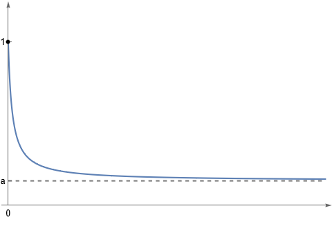
    fif_{i}, i=Ti=T, SS, are decreasing, fi(0)=1f_{i}(0)=1 and limxfi(x)=ai,x>0\lim\limits_{x\to\infty}f_{i}(x)=a_{i,x}>0, where aT,xa_{T,x}, aS,xa_{S,x} are some constants (see Fig. 1(c));

  6. 6.

    gig_{i}, i=Ti=T, SS, are increasing, gi(0)=0g_{i}(0)=0, gS(u)<gT(u)g_{S}(u)<g_{T}(u) for u>0u>0;
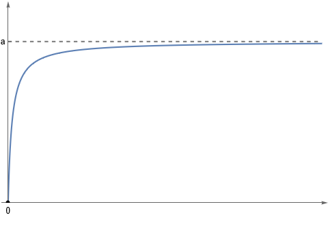
    moreover, limugi(u)\lim\limits_{u\to\infty}g_{i}(u) =ai,u>0=a_{i,u}>0, where aT,ua_{T,u}, aS,ua_{S,u} are some constants (see Fig. 1(b));

  7. 7.

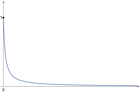
    hih_{i}, i=Ti=T, S{S}, are decreasing, hi(0)=1h_{i}(0)=1, limZhi(Z)=0\lim\limits_{Z\to\infty}h_{i}(Z)=0 (see Fig. 1(d));

  8. 8.

    fCf_{C} is increasing, limzfC(z)=aC,v>0\lim_{z\to\infty}f_{C}(z)=a_{C,v}>0 for some constant aC,va_{C,v}, fC(0)>0f_{C}^{\prime}(0)>0 and limzfC(z)=0\lim\limits_{z\to\infty}f_{C}^{\prime}(z)=0 (see Fig. 1(a)1(b));

  9. 9.

    gCg_{C} is decreasing, gC(0)=1g_{C}(0)=1 and limxgC(x)=aC,x>0\lim\limits_{x\to\infty}g_{C}(x)=a_{C,x}>0 for some constant aC,xa_{C,x} (see Fig. 1(c));

  10. 10.

    N(t)N0N(t)\equiv N\geqslant 0, i.e. the therapy is constant in time;

  11. 11.

    fx(T,S)=gx+ax,TT+ax,SSf_{x}(T,S)=g_{x}+a_{x,T}T+a_{x,S}S, fy(C)=ay,CCf_{y}(C)=a_{y,C}C, where gx,ax,Tg_{x},a_{x,T}, ax,Sa_{x,S}, ay,C>0a_{y,C}>0 are some constants;

  12. 12.

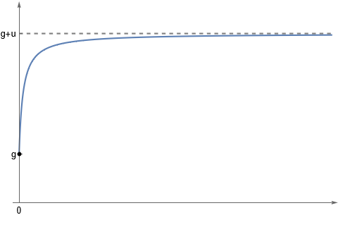
    fuf_{u} is increasing, fu(0)=gu>0f_{u}(0)=g_{u}>0 and limyfu(y)=gu+au,y\lim\limits_{y\to\infty}f_{u}(y)=g_{u}+a_{u,y}, where au,y>0a_{u,y}>0 is some constant (see Fig. 1(a));

  13. 13.

    fvf_{v} is decreasing to zero and fv(0)=1f_{v}(0)=1 (see Fig. 1(d));

  14. 14.

    gvg_{v} is increasing, gv(0)=0g_{v}(0)=0, limygv(y)=0\lim\limits_{y\to\infty}g_{v}^{\prime}(y)=0, limygv(y)=av,y>0\lim\limits_{y\to\infty}g_{v}(y)=a_{v,y}>0 for some constant av,ya_{v,y} (see Fig. 1(b)).

Refer to caption
(a) fu,f_{u}, fC.f_{C}.
Refer to caption
(b) gT,g_{T}, gS,g_{S}, fC,f_{C}, gv.g_{v}.
Refer to caption
(c) fT,f_{T}, fS,f_{S}, gC.g_{C}.
Refer to caption
(d) hT,h_{T}, hS,h_{S}, fv.f_{v}.
Figure 1: Exemplary graphs of some of the functions described in Assumption 1.

From the above assumptions, we find that the RHS of System (1) is of class 𝐂1\mathbf{C}^{1}, which guarantees the local existence and uniqueness of solutions. In [9], following the ideas of Kogan et al.[8], the authors proved the dissipativity of the System (1) and then analyzed the tumor-free steady state. However, they obtained implicit conditions of the stability, which we would like to reformulate in explicit form. For further analysis of tumor persistence states, they posed a simplifying assumption which we also exploit in our paper.

Because System (1) is highly complex, for its further analysis we introduce the following simplifying assumption.

Assumption 2.

We assume that NN is the total number of lymphocytes that enter the tumor area as a result of immunotherapy and the body’s natural immune response, i.e. Eq. (\theparentequation.3) reads

C˙=NμCC.\dot{C}=N-\mu_{C}C.

The assumption above implies that vv no longer influences other variables in the system. Thus, we can consider System (1) without the last equation. Note that for any initial conditions the variables CC, yy, and uu converge exponentially to C(N),C^{*}(N), y(N),y^{*}(N), u(N)u^{*}(N), where

C(N):=NμC,y(N):=fy(C(N))μy,u(N):=fu(y(N))μu.C^{*}(N):=\frac{N}{\mu_{C}},\;y^{*}(N):=\frac{f_{y}\big{(}C^{*}(N)\big{)}}{\mu_{y}},\;u^{*}(N):=\frac{f_{u}\big{(}y^{*}(N)\big{)}}{\mu_{u}}.

Thus, we will consider a quasi-stationary approximation for C,y,uC,y,u. Eventually, System (1) takes the following form:

T˙\displaystyle\dot{T} =rαSKSTKT(KTT)+rT(1TKT)TfT(x)GT(N)hT(T)T,\displaystyle=r_{\alpha}\frac{S}{K_{S}}\frac{T}{K_{T}}(K_{T}-T)+r_{T}\left(1-\frac{T}{K_{T}}\right)T-f_{T}(x)G_{T}(N)h_{T}(T)T, (\theparentequation.1)
S˙\displaystyle\dot{S} =rS(1SKS)SrαSKSTKT(KTT)fS(x)GS(N)hS(S)S,\displaystyle=r_{S}\left(1-\frac{S}{K_{S}}\right)S-r_{\alpha}\frac{S}{K_{S}}\frac{T}{K_{T}}(K_{T}-T)-f_{S}(x)G_{S}(N)h_{S}(S)S, (\theparentequation.2)
x˙\displaystyle\dot{x} =gx+ax,TT+ax,SSμxx,\displaystyle=g_{x}+a_{x,T}T+a_{x,S}S-\mu_{x}x, (\theparentequation.3)

where

Gi(N):=gi(u(N))C(N),i=T,S.G_{i}(N):=g_{i}\big{(}u^{*}(N)\big{)}C^{*}(N),\quad i=T,\,S.
Remark 3.

Under Assumption 2 the stability of steady states of the full System (1) and the simplified System (2) is equivalent.

The above remark allows us to note that without loss of generality it is enough to study steady states of the simplified system instead of the full one.

Now we proceed to the analysis of the properties of the functions Gi(N)G_{i}(N), i=Ti=T, SS. Based on Assumption 1 we get that

u(N)=\displaystyle u^{*}(N)= fu(y)μu=1μufu(ay,CC(N)μy)=1μufu(ay,CNμyμC)\displaystyle\frac{f_{u}(y^{*})}{\mu_{u}}=\frac{1}{\mu_{u}}f_{u}\left(\frac{a_{y,C}C^{*}(N)}{\mu_{y}}\right)=\frac{1}{\mu_{u}}f_{u}\left(\frac{a_{y,C}N}{\mu_{y}\mu_{C}}\right)

and thus

Gi(N)=gi(1μufu(ay,CNμyμC))NμC,i=T,S.G_{i}(N)=g_{i}\left(\frac{1}{\mu_{u}}f_{u}\left(\frac{a_{y,C}N}{\mu_{y}\mu_{C}}\right)\right)\frac{N}{\mu_{C}},\quad i=T,\,S.

Since the functions fuf_{u} and gig_{i}, i=Ti=T, SS, are increasing and nonnegative, so are the functions GiG_{i}, i=Ti=T, SS. Moreover,

Gi(N)=0N=0,i=T,S,G_{i}(N)=0\iff N=0,\quad i=T,\,S,

and

limNGi(N)=,i=T,S.\lim_{N\rightarrow\infty}G_{i}(N)=\infty,\quad i=T,\,S.

Because limugi(u)=ai,u\lim_{u\rightarrow\infty}g_{i}(u)=a_{i,u} and gig_{i} are increasing, i=Ti=T, SS, we get that

limNGi(N)N=limNgi(1μufu(ay,CNμyμC))1μCai,uμC,i=T,S.\lim_{N\rightarrow\infty}\frac{G_{i}(N)}{N}=\lim_{N\rightarrow\infty}g_{i}\left(\frac{1}{\mu_{u}}f_{u}\left(\frac{a_{y,C}N}{\mu_{y}\mu_{C}}\right)\right)\frac{1}{\mu_{C}}\leqslant\frac{a_{i,u}}{\mu_{C}},\quad i=T,\,S.

Furthermore, since u>0gT(u)>gS(u),\forall{u>0}\;\;g_{T}(u)>g_{S}(u), then the following corollary holds.

Corollary 4.

If Assumptions 1 and 2 are satisfied, then the functions GiG_{i}, i=Ti=T, SS, are strictly increasing and linearly bounded. Moreover

GT(0)=GS(0)=0andN>0GT(N)>GS(N).G_{T}(0)=G_{S}(0)=0\quad\text{and}\quad\forall{N>0}\ \ G_{T}(N)>G_{S}(N).
Proposition 5.

If Assumption 1 is satisfied, then System (2) has unique nonnegative solutions for nonnegative initial data. Moreover, if T0KTT_{0}\leq K_{T} and S0KSS_{0}\leq K_{S}, then the solutions are bounded from above and defined for all t0.t\geqslant 0.

Proof: Existence and uniqueness are a simple consequence of Assumption 1. We will now show that the solutions are nonnegative. From Equation (\theparentequation.1) we get that if T=0T=0, then T˙=0\dot{T}=0. Hence, if T0=0T_{0}=0, then T(t)=0T(t)=0 for all t0t\geqslant 0 for which the solution exists. The uniqueness of the solutions implies that if T0>0T_{0}>0, then T(t)>0T(t)>0 for all t0t\geqslant 0 for which the solution exists. The same argument applies for Eq. (\theparentequation.2).

Now, consider Eq. (\theparentequation.3). Because for x=0x=0 there is x˙=gx+ax,TT+ax,SSgx>0\dot{x}=g_{x}+a_{x,T}T+a_{x,S}S\geq g_{x}>0, the variable xx cannot take negative values for x00x_{0}\geq 0. Thus, all the coordinates of the solutions to System (2) are nonnegative.

Next, we proceed to show that the solutions to System (2) are also bounded from above. Note that

T˙\displaystyle\dot{T} rαSKSTKT(KTT)+rT(1TKT)T\displaystyle\leqslant r_{\alpha}\frac{S}{K_{S}}\frac{T}{K_{T}}(K_{T}-T)+r_{T}\left(1-\frac{T}{K_{T}}\right)T (3)
=(rαSKS+rT)T(KTT)KT.\displaystyle=\left(r_{\alpha}\frac{S}{K_{S}}+r_{T}\right)\frac{T(K_{T}-T)}{K_{T}}.

Let us assume that T0[0,KT]T_{0}\in[0,K_{T}] and there exists t1t_{1} such that T(t1)=KTT(t_{1})=K_{T} and TT exceeds KTK_{T} at t1t_{1}. Then there must exist such ϵ>0\epsilon>0 that for each t(t1,t1+ϵ)t\in(t_{1},t_{1}+\epsilon) T(t)>KT.T(t)>K_{T}. From (3) we, therefore, get T˙(t)<0\dot{T}(t)<0 for all t(t1,t1+ϵ)t\in(t_{1},t_{1}+\epsilon). On the other hand, from the Lagrange theorem there exists such ξ(t1,t1+ϵ)\xi\in(t_{1},t_{1}+\epsilon) that

T˙(ξ)=\displaystyle\dot{T}(\xi)= T(t1+ϵ)T(t1)ϵ=T(t1+ϵ)KTϵ>0,\displaystyle\frac{T(t_{1}+\epsilon)-T(t_{1})}{\epsilon}=\frac{T(t_{1}+\epsilon)-K_{T}}{\epsilon}>0,

which yields a contradiction. Thus, TKTT\leqslant K_{T}, and hence we have

S˙\displaystyle\dot{S} =rS(1SKS)SrαSKSTKT(KTT)fS(x)GS(N)hS(S)S\displaystyle=r_{S}\left(1-\frac{S}{K_{S}}\right)S-r_{\alpha}\frac{S}{K_{S}}\frac{T}{K_{T}}(K_{T}-T)-f_{S}(x)G_{S}(N)h_{S}(S)S
rS(1SKS)S.\displaystyle\leqslant r_{S}\left(1-\frac{S}{K_{S}}\right)S.

This means that SS does not exceed solutions of the logistic equation

S˙=rS(1SKS)S,\dot{S}=r_{S}\left(1-\frac{S}{K_{S}}\right)S,

which implies SKSS\leqslant K_{S}. Thus, we have

x˙=\displaystyle\dot{x}= gx+ax,TT+ax,SSμxxgx+ax,TKT+ax,SKSμxx.\displaystyle g_{x}+a_{x,T}T+a_{x,S}S-\mu_{x}x\leqslant g_{x}+a_{x,T}K_{T}+a_{x,S}K_{S}-\mu_{x}x.

Let us define

x¯:=gx+ax,TKT+ax,SKSμx.\displaystyle\bar{x}:=\frac{g_{x}+a_{x,T}K_{T}+a_{x,S}K_{S}}{\mu_{x}}.

It is easy to see that if for a given t0t\geqslant 0 we have x(t)>x¯x(t)>\bar{x}, then x˙(t)<0\dot{x}(t)<0. Hence, if x0>x¯x_{0}>\bar{x}, then x(t)x0x(t)\leqslant x_{0} for all tt for which the solution exists. If x0x¯,x_{0}\leqslant\bar{x}, then x(t)x¯x(t)\leqslant\bar{x}. Thus, xx is bounded from above by xmax:=max{x0,x¯}x_{\max}:=\max\{x_{0},\bar{x}\}.

Finally, it is easy to show that since T,T, SS and xx are bounded from above, then their derivatives are also bounded. Hence, the solutions to System (2) exist for all t0t\geqslant 0. \hfill\square

Corollary 6.

If Assumption 1 is satisfied, then the System (2) has an invariant set defined by 𝒟=[0,KT]×[0,KS]×[0,x¯]\mathcal{D}=[0,K_{T}]\times[0,K_{S}]\times[0,\bar{x}].

3 Analysis of steady states

In this section we will analyze the existence and uniqueness of selected steady states of System (2), depending on the value of NN. The steady states of System (2) solve the following system of algebraic equations

0\displaystyle 0 =rαSKSTKT(KTT)+rT(1TKT)TfT(x)GT(N)hT(T)T,\displaystyle=r_{\alpha}\frac{S^{*}}{K_{S}}\frac{T^{*}}{K_{T}}(K_{T}-T^{*})+r_{T}\left(1-\frac{T^{*}}{K_{T}}\right)T^{*}-f_{T}(x^{*})G_{T}(N)h_{T}(T^{*})T^{*}, (\theparentequation.1)
0\displaystyle 0 =rS(1SKS)SrαSKSTKT(KTT)fS(x)GS(N)hS(S)S,\displaystyle=r_{S}\left(1-\frac{S^{*}}{K_{S}}\right)S^{*}-r_{\alpha}\frac{S^{*}}{K_{S}}\frac{T^{*}}{K_{T}}(K_{T}-T^{*})-f_{S}(x^{*})G_{S}(N)h_{S}(S^{*})S^{*}, (\theparentequation.2)
0\displaystyle 0 =gx+ax,TT+ax,SSμxx.\displaystyle=g_{x}+a_{x,T}T^{*}+a_{x,S}S^{*}-\mu_{x}x^{*}. (\theparentequation.3)

In particular, if a point (T,S,x)(T^{*},S^{*},x^{*}) is a steady state of System (2), then

x=gx+ax,TT+ax,SSμx.x^{*}=\frac{g_{x}+a_{x,T}T^{*}+a_{x,S}S^{*}}{\mu_{x}}. (5)

To analyze the stability of the steady states we will use the linearization theorem. Let us denote the RHS of Eqs. (\theparentequation.1) and (\theparentequation.2) as f1f_{1} and f2f_{2}, respectively. Then the Jacobian matrix 𝒥\mathcal{J} of System (2) at any point (T,S,x)(T,S,x) reads

𝒥(T,S,x)=\displaystyle\mathcal{J}(T,S,x)= (f1T(T,S,x)f1S(T,S,x)f1x(T,S,x)f2T(T,S,x)f2S(T,S,x)f2x(T,S,x)ax,Tax,Sμx),\displaystyle\begin{pmatrix}\frac{\partial f_{1}}{\partial T}(T,S,x)&\frac{\partial f_{1}}{\partial S}(T,S,x)&\frac{\partial f_{1}}{\partial x}(T,S,x)\\[10.0pt] \frac{\partial f_{2}}{\partial T}(T,S,x)&\frac{\partial f_{2}}{\partial S}(T,S,x)&\frac{\partial f_{2}}{\partial x}(T,S,x)\\[10.0pt] a_{x,T}&a_{x,S}&-\mu_{x}\end{pmatrix}, (6)

where

f1T(T,S,x)=\displaystyle\frac{\partial f_{1}}{\partial T}(T,S,x)= rαSKTKS(KT2T)rTKTT+rT(1TKT)fT(x)GT(N)(hT(T)T+hT(T)),\displaystyle\begin{aligned} &\frac{r_{\alpha}S}{K_{T}K_{S}}(K_{T}-2T)-\frac{r_{T}}{K_{T}}T+r_{T}\left(1-\frac{T}{K_{T}}\right)\\ &-f_{T}(x)G_{T}(N)\big{(}h_{T}^{\prime}(T)T^{*}+h_{T}(T)\big{)},\end{aligned} (\theparentequation.1)
f1S(T,S,x)=\displaystyle\frac{\partial f_{1}}{\partial S}(T,S,x)= rαTKTKS(KTT),\displaystyle\,\frac{r_{\alpha}T}{K_{T}K_{S}}(K_{T}-T), (\theparentequation.2)
f1x(T,S,x)=\displaystyle\frac{\partial f_{1}}{\partial x}(T,S,x)= fT(x)GT(N)hT(T)T,\displaystyle-f_{T}^{\prime}(x)G_{T}(N)h_{T}(T)T, (\theparentequation.3)
f2T(T,S,x)=\displaystyle\frac{\partial f_{2}}{\partial T}(T,S,x)= rαSKTKS(KT2T),\displaystyle\,\frac{r_{\alpha}S}{K_{T}K_{S}}(K_{T}-2T), (\theparentequation.4)
f2S(T,S,x)=\displaystyle\frac{\partial f_{2}}{\partial S}(T,S,x)= rSKSS+rS(1SKS)rαTKTKS(KTT)fS(x)GS(N)(hS(S)S+hS(S)),\displaystyle\begin{aligned} &-\frac{r_{S}}{K_{S}}S+r_{S}\left(1-\frac{S}{K_{S}}\right)-\frac{r_{\alpha}T}{K_{T}K_{S}}(K_{T}-T)\\ &-f_{S}(x)G_{S}(N)\big{(}h_{S}^{\prime}(S)S+h_{S}(S)\big{)},\end{aligned} (\theparentequation.5)
f2x(T,S,x)=\displaystyle\frac{\partial f_{2}}{\partial x}(T,S,x)= fS(x)GS(N)hS(S)S.\displaystyle-f_{S}^{\prime}(x)G_{S}(N)h_{S}(S)S. (\theparentequation.6)

In subsequent sections, if the context makes it clear at which point we consider a partial derivative, we will often omit the point from the notation, e.g. we will write fiT\frac{\partial f_{i}}{\partial T} instead of fiT(T,S,x)\frac{\partial f_{i}}{\partial T}(T^{*},S^{*},x^{*}), i=1i=1, 22.

3.1 The case without treatment

We begin our analysis of steady states with the case of N0N\equiv 0. In this case System (4) simplifies to

0\displaystyle 0 =(rαSKS+rT)(1TKT)T,\displaystyle=\left(r_{\alpha}\frac{S^{*}}{K_{S}}+r_{T}\right)\left(1-\frac{T^{*}}{K_{T}}\right)T^{*}, (\theparentequation.1)
0\displaystyle 0 =(rS(KSS)rαTKT(KTT))SKS,\displaystyle=\left(r_{S}(K_{S}-{S^{*}})-r_{\alpha}\frac{T^{*}}{K_{T}}(K_{T}-T^{*})\right)\frac{S^{*}}{K_{S}}, (\theparentequation.2)
0\displaystyle 0 =gx+ax,TT+ax,SSμxx,\displaystyle=g_{x}+a_{x,T}T^{*}+a_{x,S}S^{*}-\mu_{x}x^{*}, (\theparentequation.3)

and it is obvious that the last coordinate satisfies Eq. (5), while Eqs. (\theparentequation.1) and (\theparentequation.2) do not depend on xx^{*}. Hence, we can analyze only the system for TT^{*} and SS^{*}.

We easily see that in a steady state

  • either T=0T^{*}=0 or T=KTT^{*}=K_{T};

  • for both the values of TT^{*}, either S=0S^{*}=0 or S=KSS^{*}=K_{S}.

Hence, there are four steady states:

A1=(0,0),A2=(0,KS),A3=(KT,0),A4=(KT,KS).A_{1}=(0,0),\quad A_{2}=(0,K_{S}),\quad A_{3}=(K_{T},0),\quad A_{4}=(K_{T},K_{S}).

To study stability of these states we use the second minor of 𝒥\mathcal{J} that reads

J2(T,S)=(rαS(KT2T)KTKS+rT(12TKT)rαT(KTT)KTKSrαS(KT2T)KTKSrS(12SKS)rαT(KTT)KTKS),J_{2}(T,S)=\begin{pmatrix}\frac{r_{\alpha}S(K_{T}-2T)}{K_{T}K_{S}}+r_{T}\left(1-\frac{2T}{K_{T}}\right)&\frac{r_{\alpha}T(K_{T}-T)}{K_{T}K_{S}}\\[20.0pt] \frac{r_{\alpha}S(K_{T}-2T)}{K_{T}K_{S}}&r_{S}\left(1-\frac{2S}{K_{S}}\right)-\frac{r_{\alpha}T(K_{T}-T)}{K_{T}K_{S}}\end{pmatrix},

and it is easy to see that for every AiA_{i}, i=1,2,3,4i=1,2,3,4, eigenvalues are real and equal to the terms on the diagonal. Therefore, in the coordinates (T,S)(T,S),

  • A1A_{1} is an unstable node, as λ1=rT>0\lambda_{1}=r_{T}>0, λ2=rS>0\lambda_{2}=r_{S}>0;

  • A2A_{2} is a saddle, as λ1=rα+rT>0\lambda_{1}=r_{\alpha}+r_{T}>0, λ2=rS<0\lambda_{2}=-r_{S}<0;

  • A3A_{3} is a saddle, as λ1=rT<0\lambda_{1}=-r_{T}<0, λ2=rS>0\lambda_{2}=r_{S}>0;

  • A4A_{4} is a stable node, as λ1=rαrT<0\lambda_{1}=-r_{\alpha}-r_{T}<0, λ2=rS<0\lambda_{2}=-r_{S}<0.

Moreover, it is also easy to see that the RHS of Eq. (\theparentequation.1) for N=0N=0 is always positive for T(0,KT)T\in(0,K_{T}), which means that T(t)KTT(t)\to K_{T} for tt\to\infty for any initial T0(0,KT)T_{0}\in(0,K_{T}). Then, it follows that S(t)KSS(t)\to K_{S} for S0(0,KS)S_{0}\in(0,K_{S}). Hence, A4A_{4} is globally stable, which implies that both populations of tumor cells grow to their maximum sizes.

In the next subsection, we will formulate the conditions that allow for a cure.

3.2 Semitrivial cure steady state

First, we consider the simplest case where T=0T^{*}=0, S=0S^{*}=0, x=gxμxx^{*}=\frac{g_{x}}{\mu_{x}}. This complete cure steady state (CCS) exists regardless of the value of NN. From Eqs. (6) and (7) we have

𝒥(0,0,gxμx)\displaystyle\mathcal{J}\left(0,0,\frac{g_{x}}{\mu_{x}}\right) =(rTfT(gxμx)GT(N)000rSfS(gxμx)GS(N)0ax,Tax,Sμx).\displaystyle=\begin{pmatrix}r_{T}-f_{T}\left(\frac{g_{x}}{\mu_{x}}\right)G_{T}(N)&0&0\\ 0&r_{S}-f_{S}\left(\frac{g_{x}}{\mu_{x}}\right)G_{S}(N)&0\\ a_{x,T}&a_{x,S}&-\mu_{x}\\ \end{pmatrix}.

Because 𝒥(0,0,gxμx)\mathcal{J}\left(0,0,\frac{g_{x}}{\mu_{x}}\right) is a lower triangular matrix its eigenvalues are

λ1\displaystyle\lambda_{1} =rTfT(gxμx)GT(N),\displaystyle=r_{T}-f_{T}\left(\frac{g_{x}}{\mu_{x}}\right)G_{T}(N), λ2\displaystyle\lambda_{2} =rSfS(gxμx)GS(N),\displaystyle=r_{S}-f_{S}\left(\frac{g_{x}}{\mu_{x}}\right)G_{S}(N), λ3\displaystyle\lambda_{3} =μx.\displaystyle=-\mu_{x}.

Of course λ3\lambda_{3} is a negative constant, while λ1\lambda_{1}, λ2<0\lambda_{2}<0 if and only if

rifi(gxμx)<Gi(N),i=T,S.\frac{r_{i}}{f_{i}\left(\frac{g_{x}}{\mu_{x}}\right)}<G_{i}(N),\quad i=T,\,S. (9)

Since the functions GiG_{i}, i=Ti=T, SS, are strictly increasing, their inverse functions Gi1G_{i}^{-1}, exist and are also strictly increasing. Thus, we can define

Nmin(i):=Gi1(rifi(gxμx)),i=T,S.N_{\min}^{(i)}:=G_{i}^{-1}\left(\frac{r_{i}}{f_{i}\left(\frac{g_{x}}{\mu_{x}}\right)}\right),\quad i=T,\,S.

It is easy to see that if N>Nminloc:=max{Nmin(T),Nmin(S)}N>N^{loc}_{\min}:=\max\left\{N_{\min}^{(T)},N_{\min}^{(S)}\right\}, then Condition (9) is satisfied, and therefore the CCS is locally asymptotically stable.

As local stability is difficult to interpret in practice, we are more interested in stronger condition of global stability. Considering System (2) in the invariant set 𝒟\mathcal{D} we can pose such conditions.

Theorem 7.

If N>NminglobN>N_{\min}^{glob}, where

Nminglob=max{GT1(rTfT(x¯)hT(KT)),GS1(rSfS(x¯)hS(KS))},N_{\min}^{glob}=\max\left\{G_{T}^{-1}\left(\frac{r_{T}}{f_{T}(\bar{x})h_{T}(K_{T})}\right),G_{S}^{-1}\left(\frac{r_{S}}{f_{S}(\bar{x})h_{S}(K_{S})}\right)\right\},

, then the CCS is globally stable in 𝒟\mathcal{D}.

Proof: First note that in the invariant set, due to monotonicity of the functions fif_{i}, hih_{i}, i=Ti=T, SS, we have

fi(x)fi(x¯),hi(i)hi(Ki),i=T,S,f_{i}(x)\geq f_{i}(\bar{x}),\quad h_{i}(i)\geq h_{i}(K_{i}),\quad i=T,\,S,

and therefore

S˙rS(1SKS)SfS(x¯)GS(N)hS(KS)SS(rSfS(x¯)GS(N)hS(KS)).\dot{S}\leq r_{S}\left(1-\frac{S}{K_{S}}\right)S-f_{S}(\bar{x})G_{S}(N)h_{S}(K_{S})S\leq S\left(r_{S}-f_{S}(\bar{x})G_{S}(N)h_{S}(K_{S})\right).

We easily see that if the coefficient r^S=rSfS(x¯)GS(N)hS(KS)\hat{r}_{S}=r_{S}-f_{S}(\bar{x})G_{S}(N)h_{S}(K_{S}) is negative, that is, GS(N)>rSfS(x¯)hS(KS)G_{S}(N)>\frac{r_{S}}{f_{S}(\bar{x})h_{S}(K_{S})}, then SS tends to 0 exponentially over time.

Similarly, if GT(N)>rTfT(x¯)hT(KT)G_{T}(N)>\frac{r_{T}}{f_{T}(\bar{x})h_{T}(K_{T})}, then the coefficient

r^T=rTfT(x¯)GT(N)hT(KT)<0,\hat{r}_{T}=r_{T}-f_{T}(\bar{x})G_{T}(N)h_{T}(K_{T})<0,

and according to the assumption of this theorem, there exists t¯>0\bar{t}>0 such that

rαS(t)KS<|r^T|2,for allt>t¯.r_{\alpha}\frac{S(t)}{K_{S}}<\frac{\left|\hat{r}_{T}\right|}{2},\quad\text{for all}\ \ t>\bar{t}.

Therefore, for t>t¯t>\bar{t},

T˙rαSKST+rTTfT(x¯)GT(N)hT(KT)T<|r^T|2T,\dot{T}\leq r_{\alpha}\frac{S}{K_{S}}{T}+r_{T}T-f_{T}(\bar{x})G_{T}(N)h_{T}(K_{T})T<-\frac{\left|\hat{r}_{T}\right|}{2}T,

implies that T(t)0T(t)\to 0 as well. Then it is obvious that x(t)xx(t)\to x^{*}. \hfill\square

3.3 Recurrence steady state

In this section, we consider a situation in which ordinary cancer cells TT have been destroyed as a result of therapy but some population of cancer stem cells SS has survived. In other words, we will analyze the steady states (0,S,x)(0,S^{*},x^{*}) such that S>0.S^{*}>0. We will call this state the RSS.

Since we assume that T=0T^{*}=0, then x=gx+ax,SSμxx^{*}=\frac{g_{x}+a_{x,S}S^{*}}{\mu_{x}}, and Eq. (\theparentequation.2) for S0S^{*}\neq 0 reads

rS(1SKS)=fS(gx+ax,SSμx)GS(N)hS(S).r_{S}\left(1-\frac{S^{*}}{K_{S}}\right)=f_{S}\left(\frac{g_{x}+a_{x,S}S^{*}}{\mu_{x}}\right)G_{S}(N)h_{S}(S^{*}). (10)

Note that the LHS of Eq. (10) is linear decreasing, taking the values in the interval [0,r2][0,r_{2}] in the invariant set 𝒟\mathcal{D}, where 0 is achieved for S=KSS^{*}=K_{S}. Let us denote the RHS of Eq. (10) by FF, that is,

F(Z)=GS(N)fS(gx+ax,SZμx)hS(Z),Z[0,KS].F(Z)=G_{S}(N)f_{S}\left(\frac{g_{x}+a_{x,S}Z}{\mu_{x}}\right)h_{S}(Z),\quad Z\in[0,K_{S}].

.

Let us fix N0N\geq 0 and consider the number of solutions to Eq. (10). It is obvious that for N=0N=0, the only solution is S=KSS^{*}=K_{S}.

For N>0N>0, the function FF takes positive values for Z0Z\geq 0. Now, we study the properties of FF. Using Assumption 1 we calculate:

  • F(0)=GS(N)fS(gxμx)(GS(N)aS,x,GS(N)]F(0)=G_{S}(N)f_{S}\left(\frac{g_{x}}{\mu_{x}}\right)\in\left(G_{S}(N)a_{S,x},G_{S}(N)\right];

  • F(Z)=GS(N)(ax,SμxfS(gx+ax,SZμx)hS(Z)+fS(gx+ax,SZμx)hS(Z))0F^{\prime}(Z)=G_{S}(N)\left(\frac{a_{x,S}}{\mu_{x}}f^{\prime}_{S}\left(\frac{g_{x}+a_{x,S}Z}{\mu_{x}}\right)h_{S}(Z)+f_{S}\left(\frac{g_{x}+a_{x,S}Z}{\mu_{x}}\right)h_{S}^{\prime}(Z)\right)\leq 0;

  • F(KS)=GS(N)fS(gx+ax,SKSμx)hS(KS)>0F(K_{S})=G_{S}(N)f_{S}\left(\frac{g_{x}+a_{x,S}K_{S}}{\mu_{x}}\right)h_{S}(K_{S})>0, limZF(Z)=0\lim\limits_{Z\to\infty}F(Z)=0.

These properties allow us to conclude the following.

Remark 8.

If rS>F(0)r_{S}>F(0), then there exists at least one RSS.

However, without specifying the shapes of fSf_{S} and hSh_{S} more precisely, we are not able to estimate this number from above. Hence, we pose additional assumptions related to these functions.

Assumption 9.

Assume that fSf_{S} and hSh_{S} are convex functions.

Remark 10.

The product of two nonnegative, decreasing, convex functions is a nonnegative, decreasing, convex function.

Using this property of the function FF, we are now in a position to study the number of RSS.

  • If F(0)<rSF(0)<r_{S}, then there is exactly one RSS. The smaller the value of F(0)F(0), the closer the solution SS^{*} is to KSK_{S}.

  • If F(0)=rSF(0)=r_{S}, then:

    (I) |F(0)|rSKS|F^{\prime}(0)|\leq\frac{r_{S}}{K_{S}}, then there is only one solution that overlaps with the CCS.

    (II) |F(0)|>rSKS|F^{\prime}(0)|>\frac{r_{S}}{K_{S}}, then there are two solutions and the smaller one overlaps with the CCS.

  • If F(0)>rSF(0)>r_{S}, then:

    (I) |F(0)|rSKS|F^{\prime}(0)|\leq\frac{r_{S}}{K_{S}}, then there is no nonnegative solution.

    (II) |F(0)|>rSKS|F^{\prime}(0)|>\frac{r_{S}}{K_{S}}, then there are two solutions until the next bifurcation, where F(0)F(0) is such that the two solutions overlap and the straight line in tangent to FF. For larger F(0)F(0), there is no solution.

One the basis of the above considerations, let us define the following critical values of NN:

NthI:=GS1(rSfS(gxμx))=Nmin(S),NthII:=GS1(rSKS|ax,SμxfS(gxμx)+fS(gxμx)hS(0)|),NthIII:=GS1(rS(1SthKS)fS(gx+ax,SSthμx)hS(Sth)),if there existsSthsatisfying\begin{split}N_{th}^{I}:=&\ G_{S}^{-1}\left(\frac{r_{S}}{f_{S}(\frac{g_{x}}{\mu_{x}})}\right)=N_{\min}^{(S)},\\ N_{th}^{II}:=&\ G_{S}^{-1}\left(\frac{r_{S}}{K_{S}\left|\frac{a_{x,S}}{\mu_{x}}f_{S}^{\prime}(\frac{g_{x}}{\mu_{x}})+f_{S}(\frac{g_{x}}{\mu_{x}})h_{S}^{\prime}(0)\right|}\right),\\ N_{th}^{III}:=&\ G_{S}^{-1}\left(\frac{r_{S}\left(1-\frac{S^{*}_{th}}{K_{S}}\right)}{f_{S}\left(\frac{g_{x}+a_{x,S}S^{*}_{th}}{\mu_{x}}\right)h_{S}(S^{*}_{th})}\right),\ \text{if there exists}\ S^{*}_{th}\ \text{satisfying}\end{split}
(KSSth)fS(gx+ax,SSthμx)hS(Sth)\displaystyle\ \frac{\left(K_{S}-{S^{*}_{th}}\right)}{f_{S}\left(\frac{g_{x}+a_{x,S}S^{*}_{th}}{\mu_{x}}\right)h_{S}(S^{*}_{th})} =1|ax,SμxfS(gx+ax,SSthμx)hS(Sth)+fS(gx+ax,SSthμx)hS(Sth)|.\displaystyle=\frac{1}{\left|\frac{a_{x,S}}{\mu_{x}}f_{S}^{\prime}(\frac{g_{x}+a_{x,S}S^{*}_{th}}{\mu_{x}})h_{S}(S^{*}_{th})+f_{S}(\frac{g_{x}+a_{x,S}S^{*}_{th}}{\mu_{x}})h_{S}^{\prime}(S^{*}_{th})\right|}.

Now, we are ready to formulate the following theorem.

Theorem 11.

For System (2), under Assumption 9, the number of the RSS varies from 0 to 2.

  1. 1.

    If N<NthIN<N_{th}^{I}, then there is exactly one RSS.

  2. 2.

    At N=NthIN=N_{th}^{I} there is a bifurcation.

  3. 3.

    If NthI<NthIIN^{I}_{th}<N_{th}^{II}, then for N(NthI,NthII]N\in\left(N_{th}^{I},N_{th}^{II}\right] there is no RSS.

  4. 4.

    If NthI>NthIIN^{I}_{th}>N_{th}^{II}, then for N>NthIN>N_{th}^{I} there are two RSS until the next bifurcation at N=NthIIIN=N^{III}_{th}.

  5. 5.

    If N>NthIIIN>N_{th}^{III}, then there is no RSS.

Remark 12.

If we additionally assume Ks>1K_{s}>1 (an obvious assumption in reality) and h(0)=1h^{\prime}(0)=-1, then we can exclude Case 3. in the above theorem due to the inequality NthII<NthIN_{th}^{II}<N_{th}^{I}.

To gain a bit deeper insight into the existence and stability of the RSS and coexistence steady states, and to perform numerical simulations, in the following we introduce an additional assumption about the explicit forms of functions appearing in System (2).

Assumption 13.

From now on we assume that

  1. 1.

    fT(x)=aT,xx+1x+1f_{T}(x)=\frac{a_{T,x}x+1}{x+1} (decreasing if aT,x(0,1),a_{T,x}\in(0,1), fT(0)=1,f_{T}(0)=1, limxfT(x)=aT,x\lim_{x\rightarrow\infty}f_{T}(x)=a_{T,x}),

  2. 2.

    gT(u)=aT,uuu+1g_{T}(u)=\frac{a_{T,u}u}{u+1} (increasing, limugT(u)=aT,u\lim_{u\rightarrow\infty}g_{T}(u)=a_{T,u}),

  3. 3.

    hT(T)=1T+1h_{T}(T)=\frac{1}{T+1} (decreasing, hT(0)=1h_{T}(0)=1, limThT(T)=0\lim_{T\rightarrow\infty}h_{T}(T)=0),

  4. 4.

    fS(x)=aS,xx+1x+1f_{S}(x)=\frac{a_{S,x}x+1}{x+1} (decreasing if aS,x(0,1),a_{S,x}\in(0,1), fS(0)=1,f_{S}(0)=1, limxfS(x)=aS,x\lim_{x\rightarrow\infty}f_{S}(x)=a_{S,x}),

  5. 5.

    gS(u)=aS,uuu+1g_{S}(u)=\frac{a_{S,u}u}{u+1} (increasing, limugS(u)=aS,u\lim_{u\rightarrow\infty}g_{S}(u)=a_{S,u}),

  6. 6.

    hS(S)=1S+1h_{S}(S)=\frac{1}{S+1} (decreasing, hS(0)=1h_{S}(0)=1, limThS(S)=0\lim_{T\rightarrow\infty}h_{S}(S)=0),

  7. 7.

    fC(z)=aC,vzz+1f_{C}(z)=\frac{a_{C,v}z}{z+1} (increasing, limzfC(z)=aC,v\lim_{z\rightarrow\infty}f_{C}(z)=a_{C,v}, fC(0)>0f_{C}^{\prime}(0)>0, limzfC(z)=0,\lim_{z\rightarrow\infty}f_{C}^{\prime}(z)=0, where z=(T+S)vz=(T+S)v),

  8. 8.

    gC(x)=aC,xx+1x+1g_{C}(x)=\frac{a_{C,x}x+1}{x+1} (decreasing for aC,x(0,1),a_{C,x}\in(0,1), gC(0)=1g_{C}(0)=1, limxgC(x)\lim_{x\rightarrow\infty}g_{C}(x)),

  9. 9.

    fu(y)=au,yyy+1+guf_{u}(y)=\frac{a_{u,y}y}{y+1}+g_{u} (increasing, fu(0)=gu,f_{u}(0)=g_{u}, limyfu(z)=au,y\lim_{y\rightarrow\infty}f_{u}(z)=a_{u,y}),

  10. 10.

    fv(x)=1x+1f_{v}(x)=\frac{1}{x+1} (decreasing, fv(0)=1,f_{v}(0)=1, limxfv(x)=0\lim_{x\rightarrow\infty}f_{v}(x)=0),

  11. 11.

    gv(y)=av,yyy+1g_{v}(y)=\frac{a_{v,y}y}{y+1} (increasing, gv(0)=0,g_{v}(0)=0, limygv(y)=av,y,\lim_{y\rightarrow\infty}g_{v}(y)=a_{v,y}, limygv(y)=0\lim_{y\rightarrow\infty}g_{v}^{\prime}(y)=0).

We now reformulate conditions for the existence of RSS under Assumptions 13. Since we assume that T=0,T^{*}=0, then Eq. (\theparentequation.1) reads

0\displaystyle 0 =R2(S)SfS(x)G2(N)hS(S)S.\displaystyle=R_{2}(S^{*})S^{*}-f_{S}(x^{*})G_{2}(N)h_{S}(S^{*})S^{*}. (11)
Refer to caption
(a) N=0N=0
Refer to caption
(b) H(0;N)<F(0)H(0;N)<F(0)
Refer to caption
(c) H(0;N)=F(0),H(0;N)=F(0), H(0;N)<F(0)H^{\prime}(0;N)<F^{\prime}(0)
Refer to caption
(d) H(0;N)F(0),H(0;N)F(0)H(0;N)\geqslant F(0),H^{\prime}(0;N)\geqslant F^{\prime}(0)
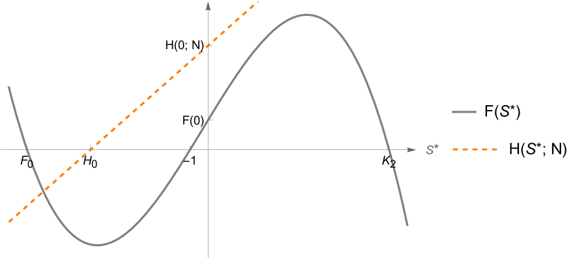
Figure 2: Sample plots of H(S;N)H(S^{*};N) and F(S)F(S^{*}) depending on the value of the parameter NN.

We divide both sides of Eq. (11) by S>0S^{*}>0 and substitute Eq. (5) to obtain

0\displaystyle 0 =rSKSSKSaS,x(gx+ax,SS)+μxgx+ax,SS+μx1S+1GS(N).\displaystyle=r_{S}\frac{K_{S}-S^{*}}{K_{S}}-\frac{a_{S,x}(g_{x}+a_{x,S}S^{*})+\mu_{x}}{g_{x}+a_{x,S}S^{*}+\mu_{x}}\frac{1}{S^{*}+1}G_{S}(N). (12)

By reducing the RHS of Eq. (12) to the common denominator and taking only the numerator we get the equivalent equation that reads

rS(KSS)(gx+ax,SS+μx)(S+1)=KS(aS,x(gx+ax,SS)+μx)GS(N).\displaystyle r_{S}(K_{S}-S^{*})(g_{x}+a_{x,S}S^{*}+\mu_{x})(S^{*}+1)=K_{S}(a_{S,x}(g_{x}+a_{x,S}S^{*})+\mu_{x})G_{S}(N). (13)

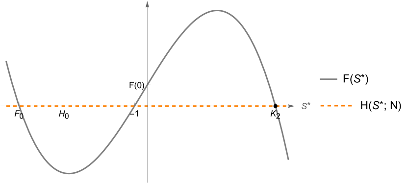
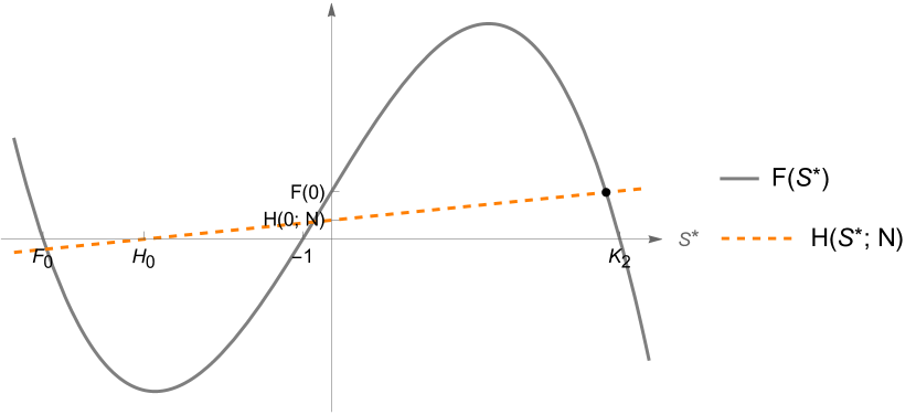
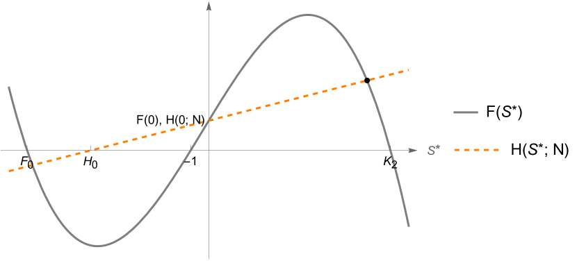
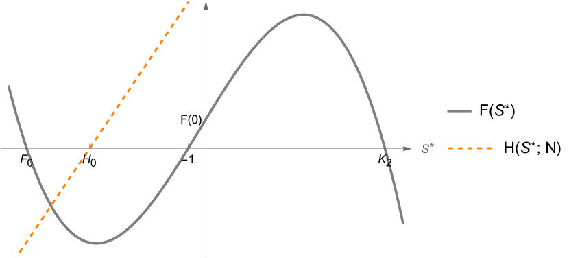
Let F(S),F(S^{*}), H(S;N)H(S^{*};N) denote the LHS and RHS of Eq. (13), respectively. Of course, F(S)F(S^{*}) is a third degree polynomial of S,S^{*}, while H(S;N)H(S^{*};N) is a first-degree polynomial of SS^{*} with NN as a parameter. Note that finding the number of RSSs depending on the value of NN is equivalent to finding the number of points at which the graphs of FF and HH intersect for S>0S^{*}>0 depending on the value of NN. The set of roots of F(S)F(S^{*}) reads

0={gx+μxax,S,1,KS},\displaystyle\mathcal{F}^{0}=\left\{-\frac{g_{x}+\mu_{x}}{a_{x,S}},-1,K_{S}\right\},

while the only root of H(S;N)H(S^{*};N) is equal to

μx+gxaS,xax,SaS,x.-\frac{\mu_{x}+g_{x}a_{S,x}}{a_{x,S}a_{S,x}}.

We easily see that

F(0)=\displaystyle F(0)= rSKS(gx+μx),\displaystyle\;r_{S}K_{S}(g_{x}+\mu_{x}), (\theparentequation.1)
F(0)=\displaystyle F^{\prime}(0)= rS((gx+μx)(KS1)+KSax,S),\displaystyle\;r_{S}\Big{(}(g_{x}+\mu_{x})(K_{S}-1)+K_{S}a_{x,S}\Big{)}, (\theparentequation.2)
H(0;N)=\displaystyle H(0;N)= GS(N)KS(aS,xgx+μx),\displaystyle\;G_{S}(N)K_{S}(a_{S,x}g_{x}+\mu_{x}), (\theparentequation.3)
H(0;N)=\displaystyle H^{\prime}(0;N)= GS(N)KSaS,xax,S.\displaystyle\;G_{S}(N)K_{S}a_{S,x}a_{x,S}. (\theparentequation.4)

As we have noticed before in the general case, in reality we have KS1K_{S}\gg 1, and therefore F(0)>0F^{\prime}(0)>0. This implies that the third-degree polynomial FF is concave for S>0S^{*}>0, since F(0)F(0) is positive.

Refer to caption
(a) H(0)>F(0)H(0)>F(0), H<F(0),N>NcritH^{\prime}<F^{\prime}(0),N>N_{\text{crit}}
Refer to caption
(b) H(0)>F(0)H(0)>F(0), H<F(0),N=NcritH^{\prime}<F^{\prime}(0),N=N_{\text{crit}}
Refer to caption
(c) H(0)>F(0)H(0)>F(0), H<F(0),N<NcritH^{\prime}<F^{\prime}(0),N<N_{\text{crit}}
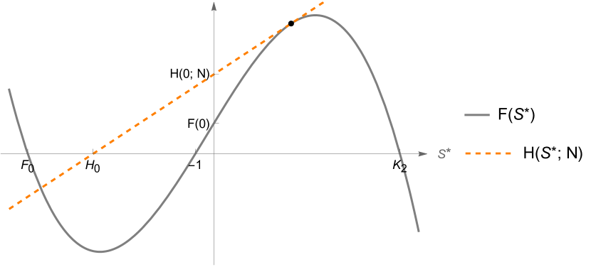
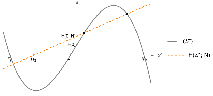
Figure 3: Sample plots of H(S;N)H(S^{*};N) and F(S)F(S^{*}) depending on the value of the parameter N;N; illustration of a bifurcation when the number of steady states changes from 0,0, through 1,1, to 2.2.

In this case, if H(0;N)<F(0),H(0;N)<F(0), then the graphs of FF and HH will intersect exactly once for S>0,S^{*}>0, see Figs 2(a)2(b), as well as if H(0;N)=F(0)H(0;N)=F(0) and H(0;N)<F(0),H^{\prime}(0;N)<F^{\prime}(0), see Fig. 2(c). However, if H(0;N)F(0)H(0;N)\geqslant F(0) and H(0;N)F(0),H^{\prime}(0;N)\geqslant F^{\prime}(0), then the graphs of FF and HH will not intersect for S>0,S^{*}>0, see Fig. 2(d).

If conditions H(0;N)>F(0)H(0;N)>F(0) and H(0;N)<F(0)H^{\prime}(0;N)<F^{\prime}(0) are met for some nonnegative N0N_{0}, then there exists an open interval II such that N0IN_{0}\in I and H(0;N)>F(0),H(0;N)>F(0), H(0;N)<F(0)H^{\prime}(0;N)<F^{\prime}(0) for all NI.N\in I. Furthermore, there exists NcritIN_{\text{crit}}\in I for which the graph of HH is tangent to the graph of FF at some Scrit,S^{*}_{\text{crit}}, i.e. the graphs of HH and FF intersect at exactly one point for S>0,S^{*}>0, see Fig. 3(b). Furthermore, if NIN\in I and N<Ncrit,N<N_{\text{crit}}, then the graphs of HH and FF intersect twice for S>0,S^{*}>0, see Fig. 3(c). On the other hand, if NIN\in I and N>Ncrit,N>N_{\text{crit}}, then the graphs of HH and FF do not intersect for S>0,S^{*}>0, see Fig. 3(a).

In order to find NcritN_{\text{crit}} and ScritS^{*}_{\text{crit}} let us solve the system

H(T;N)\displaystyle H(T^{*};N) =F(T),\displaystyle=F(T^{*}),
H(T;N)\displaystyle H^{\prime}(T^{*};N) =F(T),\displaystyle=F^{\prime}(T^{*}),

which is equivalent to

KS(aS,x(gx+ax,SS)+μx)GS(N)\displaystyle K_{S}\big{(}a_{S,x}(g_{x}+a_{x,S}S^{*})+\mu_{x}\big{)}G_{S}(N) =F(S),\displaystyle=F(S^{*}), (\theparentequation.1)
KSaS,xax,SGS(N)\displaystyle K_{S}a_{S,x}a_{x,S}G_{S}(N) =F(S).\displaystyle=F^{\prime}(S^{*}). (\theparentequation.2)

From Eq. (\theparentequation.2) we get

GS(N)=F(S)KSaS,xax,S\begin{gathered}G_{S}(N)=\frac{F^{\prime}(S^{*})}{K_{S}a_{S,x}a_{x,S}}\end{gathered} (16)

and after substituting Eq. (16) into Eq. (\theparentequation.1) we obtain

F(S)aS,xax,S(aS,x(gx+ax,SS)+μx)F(S)=0.\begin{gathered}\frac{F^{\prime}(S^{*})}{a_{S,x}a_{x,S}}\Big{(}a_{S,x}(g_{x}+a_{x,S}S^{*})+\mu_{x}\Big{)}-F(S^{*})=0.\end{gathered} (17)

Of course, the LHS of Eq. (17) is a third-degree polynomial so we can obtain its roots analytically. Let us denote them as w0,w1,w2.w_{0},w_{1},w_{2}. Since we know that there exists exactly one positive SS^{*} that solves Eq. (15), then we will obtain ScritS^{*}_{\text{crit}} by taking

Scrit=max{(w0),(w1),(w2)}.\displaystyle S^{*}_{\text{crit}}=\max\left\{\Re(w_{0}),\Re(w_{1}),\Re(w_{2})\right\}. (18)

On the other hand, applying GS1G_{S}^{-1} to both sides of Eq. (16) we obtain

Ncrit\displaystyle N_{\text{crit}} =GS1(F(Scrit)KSaS,xax,S).\displaystyle=G_{S}^{-1}\left(\frac{F^{\prime}(S^{*}_{\text{crit}})}{K_{S}a_{S,x}a_{x,S}}\right).
Corollary 14.

The number of the RSS of System (2) under Assumption 13 is dependent on the value of the parameter NN in the following way. For N0N\geqslant 0 such that

  1. 1.

    H(0;N)F(0)H(0;N)\geqslant F(0) and H(0;N)F(0)H^{\prime}(0;N)\geqslant F^{\prime}(0) there are no RSS;

  2. 2.

    H(0;N)<F(0)H(0;N)<F(0) or H(0;N)=F(0)H(0;N)=F(0) and H(0;N)<F(0)H^{\prime}(0;N)<F^{\prime}(0) there is exactly one RSS;

  3. 3.

    H(0;N)>F(0)H(0;N)>F(0) and H(0;N)<F(0)H^{\prime}(0;N)<F(0) and

    1. (a)

      N>NcritN>N_{\text{crit}} there are no RSS;

    2. (b)

      N=NcritN=N_{\text{crit}} there is exactly one RSS;

    3. (c)

      N<NcritN<N_{\text{crit}} there are two RSS.

Let us now proceed to analyze the RSS stability. From Eq. (6) we have

𝒥(0,S,x)\displaystyle\mathcal{J}(0,S^{*},x^{*}) =(f1T(0,S,x)00f2T(0,S,x)f2S(0,S,x)f2x(0,S,x)ax,Tax,Sμx)\displaystyle=\begin{pmatrix}\frac{\partial f_{1}}{\partial T}(0,S^{*},x^{*})&0&0\\[8.61108pt] \frac{\partial f_{2}}{\partial T}(0,S^{*},x^{*})&\frac{\partial f_{2}}{\partial S}(0,S^{*},x^{*})&\frac{\partial f_{2}}{\partial x}(0,S^{*},x^{*})\\[8.61108pt] a_{x,T}&a_{x,S}&-\mu_{x}\end{pmatrix} (19)

The characteristic polynomial of 𝒥(0,S,x)\mathcal{J}(0,S^{*},x^{*}) is given as

W(λ)\displaystyle W(\lambda) =(f1Tλ)(λ2+λ(μxf2S)(μxf2S+ax,Sf2x)).\displaystyle=\left(\frac{\partial f_{1}}{\partial T}-\lambda\right)\left(\lambda^{2}+\lambda\left(\mu_{x}-\frac{\partial f_{2}}{\partial S}\right)-\left(\mu_{x}\frac{\partial f_{2}}{\partial S}+a_{x,S}\frac{\partial f_{2}}{\partial x}\right)\right).

Let us denote

V(λ):=λ2+λ(μxf2S)(μxf2S+ax,Sf2x)\begin{gathered}V(\lambda):=\lambda^{2}+\lambda\left(\mu_{x}-\frac{\partial f_{2}}{\partial S}\right)-\left(\mu_{x}\frac{\partial f_{2}}{\partial S}+a_{x,S}\frac{\partial f_{2}}{\partial x}\right)\end{gathered} (20)

and let v1,v2v_{1},v_{2} be the roots of V(λ).V(\lambda). Of course, if all the eigenvalues of 𝒥(0,S,x),\mathcal{J}(0,S^{*},x^{*}), i.e. f1T,v1,v2,\frac{\partial f_{1}}{\partial T},v_{1},v_{2}, have negative real parts, then the RSS is locally asymptotically stable. Note that from Eq. (5) and Assumption 13 we obtain

f1T(0,S,x)\displaystyle\frac{\partial f_{1}}{\partial T}(0,S^{*},x^{*}) =rαSKS+rTaT,x(gx+ax,SS)+μxgx+ax,SS+μxGT(N)\displaystyle=\frac{r_{\alpha}S^{*}}{K_{S}}+r_{T}-\frac{a_{T,x}(g_{x}+a_{x,S}S^{*})+\mu_{x}}{g_{x}+a_{x,S}S^{*}+\mu_{x}}G_{T}(N) (21)
=rαSKS+rT(aT,x+(1aT,x)μxgx+ax,SS+μx)GT(N).\displaystyle=\frac{r_{\alpha}S^{*}}{K_{S}}+r_{T}-\left(a_{T,x}+\frac{(1-a_{T,x})\mu_{x}}{g_{x}+a_{x,S}S^{*}+\mu_{x}}\right)G_{T}(N).

It is easy to see that for the values of NN close to 0 the negative component of the RHS of Eq. (21) is also close to 0 and thus f1T>0.\frac{\partial f_{1}}{\partial T}>0. On the other hand, assuming aT,x1a_{T,x}\leq 1 and remembering that SKSS^{*}\leq K_{S} we see that it is enough to require GT(N)>rα+rTaT,xG_{T}(N)>\frac{r_{\alpha}+r_{T}}{a_{T,x}} to get f1T<0.\frac{\partial f_{1}}{\partial T}<0.

Note also that for the RSS we can determine the value of NN as a function of S.S^{*}. From the condition H(S;N)=F(S)H(S^{*};N)=F(S^{*}) we get

KS(aS,x(gx+ax,SS)+μx)GS(N)=F(S),\begin{gathered}K_{S}(a_{S,x}(g_{x}+a_{x,S}S^{*})+\mu_{x})G_{S}(N)=F(S^{*}),\\ \end{gathered}

or equivalently

N\displaystyle N =GS1(F(S)KS(aS,x(gx+ax,SS)+μx)).\displaystyle=G_{S}^{-1}\left(\frac{F(S^{*})}{K_{S}(a_{S,x}(g_{x}+a_{x,S}S^{*})+\mu_{x})}\right). (22)

From Corollary 4 and Eq. (21) we can deduce that

f1T(0,S,x)\displaystyle\frac{\partial f_{1}}{\partial T}(0,S^{*},x^{*}) rαSKS+rTaT,x(gx+ax,SS)+μxgx+ax,SS+μxGS(N).\displaystyle\leqslant\frac{r_{\alpha}S^{*}}{K_{S}}+r_{T}-\frac{a_{T,x}(g_{x}+a_{x,S}S^{*})+\mu_{x}}{g_{x}+a_{x,S}S^{*}+\mu_{x}}G_{S}\left(N\right). (23)
Assumption 15.

From now on, we assume that aT,x=aS,x.a_{T,x}=a_{S,x}.

From the Assumption above and Eq. (22) we get

aT,x(gx+ax,SS)+μxgx+ax,SS+μxGS(N)\displaystyle\frac{a_{T,x}(g_{x}+a_{x,S}S^{*})+\mu_{x}}{g_{x}+a_{x,S}S^{*}+\mu_{x}}G_{S}(N) =rS(KSS)(S+1)KS,\displaystyle=\frac{r_{S}(K_{S}-S^{*})(S^{*}+1)}{K_{S}}, (24)

which implies that

f1T(0,S,x)\displaystyle\frac{\partial f_{1}}{\partial T}(0,S^{*},x^{*}) rαS+rTKSrS(KSS)(S+1)KS.\displaystyle\leqslant\frac{r_{\alpha}S^{*}+r_{T}K_{S}-r_{S}(K_{S}-S^{*})(S^{*}+1)}{K_{S}}. (25)

Let us denote the numerator of the RHS of the inequality above as

Q(S)\displaystyle Q(S^{*}) :=rαS+rTKSrS(KSS)(S+1)\displaystyle:=r_{\alpha}S^{*}+r_{T}K_{S}-r_{S}(K_{S}-S^{*})(S^{*}+1)
=rSS2+S(rSrSKS+rα)+KS(rTrS).\displaystyle\ =r_{S}S^{*2}+S^{*}(r_{S}-r_{S}K_{S}+r_{\alpha})+K_{S}(r_{T}-r_{S}).

Then we have

Q(S)<0f1T(0,S,x)<0.\displaystyle Q(S^{*})<0\implies\frac{\partial f_{1}}{\partial T}(0,S^{*},x^{*})<0. (26)

Notice that the above condition can be satisfied only for small values of SS^{*}, since for SS^{*} near KSK_{S} the positive terms of Q(S)Q(S^{*}) are much larger compared to the negative one. Coming back to Formula (20), to get stability of the RSS it is enough to assume

f2Sμx\displaystyle\frac{\partial f_{2}}{\partial S}-\mu_{x} <0\displaystyle<0\quad μxf2SaS,xf2x\displaystyle\land\quad-\mu_{x}\frac{\partial f_{2}}{\partial S}-a_{S,x}\frac{\partial f_{2}}{\partial x} >0.\displaystyle>0. (27)

We have

f2Sμx\displaystyle\frac{\partial f_{2}}{\partial S}-\mu_{x} =rS(12SKS)GS(N)fS(x)1(S+1)2μx,\displaystyle=r_{S}\Big{(}1-\frac{2S^{*}}{K_{S}}\Big{)}-G_{S}(N)f_{S}(x^{*})\frac{1}{(S^{*}+1)^{2}}-\mu_{x},

and note that to have the first inequality in (27) satisfied it is enough to assume rSμxr_{S}\leq\mu_{x}. In the more general case, substituting GS(N)G_{S}(N) we obtain

f2Sμx\displaystyle\frac{\partial f_{2}}{\partial S}-\mu_{x} =rS(12SKS)F(S)KS(gx+ax,TT+ax,SS+μx)(S+1)2μx\displaystyle=r_{S}\Big{(}1-\frac{2S^{*}}{K_{S}}\Big{)}-\frac{F(S^{*})}{K_{S}(g_{x}+a_{x,T}T^{*}+a_{x,S}S^{*}+\mu_{x})(S^{*}+1)^{2}}-\mu_{x}
=rS(KS2S)(S+1)rS(KSS)μxKS(S+1)KS(S+1).\displaystyle=\frac{r_{S}(K_{S}-2S^{*})(S^{*}+1)-r_{S}(K_{S}-S^{*})-\mu_{x}K_{S}(S^{*}+1)}{K_{S}(S^{*}+1)}.

Let us denote the numerator of the expression above as

P(S)\displaystyle P(S^{*}) :=rS(KS2S)(S+1)rS(KSS)μxKS(S+1)\displaystyle:=r_{S}(K_{S}-2S^{*})(S^{*}+1)-r_{S}(K_{S}-S^{*})-\mu_{x}K_{S}(S^{*}+1)
=2rSS2+S(rS(KS1)μxKS)μxKS.\displaystyle\ =-2r_{S}{S^{*}}^{2}+S^{*}\big{(}r_{S}(K_{S}-1)-\mu_{x}K_{S}\big{)}-\mu_{x}K_{S}.

Then

f2Sμx<0P(S)<0.\begin{gathered}\frac{\partial f_{2}}{\partial S}-\mu_{x}<0\iff P(S^{*})<0.\end{gathered}

It is obvious that P(S)<0P(S^{*})<0 for the values of SS^{*} exceeding KS2\frac{K_{S}}{2}. Moreover, since

f2x\displaystyle\frac{\partial f_{2}}{\partial x} =fS(x)GS(N)hS(S)S=aS,x1(x+1)2GS(N)SS+1\displaystyle=-f_{S}^{\prime}(x^{*})G_{S}(N)h_{S}(S^{*})S^{*}=-\frac{a_{S,x}-1}{(x^{*}+1)^{2}}G_{S}(N)\frac{S^{*}}{S^{*}+1}
=μxrS(1aS,x)S(KSS)KS(gx+ax,SS+μx)(aS,x(gx+ax,SS)+μx),\displaystyle=\frac{\mu_{x}r_{S}(1-a_{S,x})S^{*}(K_{S}-S^{*})}{K_{S}(g_{x}+a_{x,S}S^{*}+\mu_{x})(a_{S,x}(g_{x}+a_{x,S}S^{*})+\mu_{x})},

then

μxf2SaS,xf2x=\displaystyle-\mu_{x}\frac{\partial f_{2}}{\partial S}-a_{S,x}\frac{\partial f_{2}}{\partial x}= μxrS(KSS)rS(KS2S)(S+1)KS(S+1)\displaystyle\mu_{x}\frac{r_{S}(K_{S}-S^{*})-r_{S}(K_{S}-2S^{*})(S^{*}+1)}{K_{S}(S^{*}+1)}
+aS,xμxrS(aS,x1)S(KSS)KS(gx+ax,SS+μx)(aS,x(gx+ax,SS)+μx).\displaystyle+a_{S,x}\frac{\mu_{x}r_{S}(a_{S,x}-1)S^{*}(K_{S}-S^{*})}{K_{S}(g_{x}+a_{x,S}S^{*}+\mu_{x})(a_{S,x}(g_{x}+a_{x,S}S^{*})+\mu_{x})}.

After reducing the RHS of the equation above to a common denominator, we can denote its numerator as

B(S):=\displaystyle B(S^{*}):= S(2S+1KS)(gx+ax,SS+μx)(aS,x(gx+ax,SS)+μx)\displaystyle S^{*}(2{S^{*}}+1-K_{S})(g_{x}+a_{x,S}S^{*}+\mu_{x})\big{(}a_{S,x}(g_{x}+a_{x,S}S^{*})+\mu_{x}\big{)}
aS,x(1aS,x)S(KSS)(S+1).\displaystyle-a_{S,x}(1-a_{S,x})S^{*}(K_{S}-S^{*})(S^{*}+1).

Thus,

μxf2SaS,xf2x>0B(S)>0.\begin{gathered}-\mu_{x}\frac{\partial f_{2}}{\partial S}-a_{S,x}\frac{\partial f_{2}}{\partial x}>0\iff B(S^{*})>0.\end{gathered}

Note that B(S)<0B(S^{*})<0 for small values of SS^{*}.

Corollary 16.

The RSS of System (2) is locally asymptotically stable if Q(S)<0Q(S^{*})<0, P(S)<0P(S^{*})<0, and B(S)>0.B(S^{*})>0.

3.4 Coexistence steady states

Now we will consider a situation in which a certain population of both types of cancer cells survives, i.e. we will analyze the existence and stability of positive steady states (T,S,x).(T^{*},S^{*},x^{*}). To be consistent with the previous subsections, we will call this state the PSS.

Recall that if N=0N=0, then System (4) simplifies to (8) and the only positive solution to it is

(KT,KS,xKT,KS)=(KT,KS,gx+ax,TKT+ax,SKSμx),\big{(}K_{T},K_{S},x^{*}_{K_{T},K_{S}}\big{)}=\Big{(}K_{T},K_{S},\frac{g_{x}+a_{x,T}K_{T}+a_{x,S}K_{S}}{\mu_{x}}\Big{)}, (28)

which is a stable node. Since System (2) depends continuously on NN, for the values of NN sufficiently close to 0 there should also exist a locally asymptotically stable steady state (T,S,x)(T^{*},S^{*},x^{*}) with T,S>0T^{*},S^{*}>0. Moreover, the coordinates TT^{*}, SS^{*} remain close to KTK_{T} and KSK_{S}, respectively.

We will now state the conditions necessary for the point (S,T,x),(S^{*},T^{*},x^{*}), S,T>0S^{*},T^{*}>0 to be the solution to System (4). Adding the first two equations of System (4) by sides we get

rT(T)T+fT(x)GT(N)hT(T)T=rS(S)SfS(x)GS(N)hS(S)S.\begin{gathered}-r_{T}(T^{*})T^{*}+f_{T}(x^{*})G_{T}(N)h_{T}(T^{*})T^{*}=r_{S}(S^{*})S^{*}-f_{S}(x^{*})G_{S}(N)h_{S}(S^{*})S^{*}.\end{gathered} (29)

In particular, Equation (29) holds when both sides are equal to 0, that is

GT(N)\displaystyle G_{T}(N) =rT(KTT)KTfT(x)hT(T),\displaystyle=\frac{r_{T}(K_{T}-T^{*})}{K_{T}f_{T}(x^{*})h_{T}(T^{*})}, GS(N)\displaystyle G_{S}(N) =rS(KSS)KSfS(x)hS(S).\displaystyle=\frac{r_{S}(K_{S}-S^{*})}{K_{S}f_{S}(x^{*})h_{S}(S^{*})}. (30)

By substituting (30) into System (4) we get

0\displaystyle 0 =rαTSKTKS(KTT),\displaystyle=\frac{r_{\alpha}T^{*}S^{*}}{K_{T}K_{S}}(K_{T}-T^{*}),
0\displaystyle 0 =rαTSKTKS(KTT),\displaystyle=-\frac{r_{\alpha}T^{*}S^{*}}{K_{T}K_{S}}(K_{T}-T^{*}),
0\displaystyle 0 =gx+ax,TT+ax,SSμxx.\displaystyle=g_{x}+a_{x,T}T^{*}+a_{x,S}S^{*}-\mu_{x}x^{*}.

Since T,S>0T^{*},S^{*}>0, solutions to the system above must have the form

(T,S,x)=(KT,S,gx+ax,TKT+ax,SSμx),\big{(}T^{*},S^{*},x^{*}\big{)}=\Big{(}K_{T},S^{*},\frac{g_{x}+a_{x,T}K_{T}+a_{x,S}S^{*}}{\mu_{x}}\Big{)}, (31)

where S>0S^{*}>0. Substituting (31) into System (30) we get

GT(N)\displaystyle G_{T}(N) =0,\displaystyle=0, GS(N)\displaystyle G_{S}(N) =rS(KSS)KSfS(x)hS(S).\displaystyle=\frac{r_{S}(K_{S}-S^{*})}{K_{S}f_{S}(x^{*})h_{S}(S^{*})}. (32)

From Corollary 4 we conclude that Condition (32) holds if and only if N=0,N=0, S=0S^{*}=0, but we have already analyzed this case.

Thus, let us assume that both sides of Equation (29) are different from 0. In this case, both sides need to be of the same sign. Both sides of this equation are positive if and only if

GT(N)\displaystyle G_{T}(N) >rT(KTT)KTfT(x)hT(T),\displaystyle>\frac{r_{T}(K_{T}-T^{*})}{K_{T}f_{T}(x^{*})h_{T}(T^{*})}, GS(N)\displaystyle G_{S}(N) <rS(KSS)KSfS(x)hS(S),\displaystyle<\frac{r_{S}(K_{S}-S^{*})}{K_{S}f_{S}(x^{*})h_{S}(S^{*})},

and both sides are negative if and only if

GT(N)\displaystyle G_{T}(N) <rT(KTT)KTfT(x)hT(T),\displaystyle<\frac{r_{T}(K_{T}-T^{*})}{K_{T}f_{T}(x^{*})h_{T}(T^{*})}, GS(N)\displaystyle G_{S}(N) >rS(KSS)KSfS(x)hS(S).\displaystyle>\frac{r_{S}(K_{S}-S^{*})}{K_{S}f_{S}(x^{*})h_{S}(S^{*})}. (33)

Note that since N>0GT(N)>GS(N),\forall{N>0}\;G_{T}(N)>G_{S}(N), then Condition (33) does not hold for any NN if

rS(KSS)KSfS(x)hS(S)rT(KTT)KTfT(x)hT(T).\frac{r_{S}(K_{S}-S^{*})}{K_{S}f_{S}(x^{*})h_{S}(S^{*})}\geqslant\frac{r_{T}(K_{T}-T^{*})}{K_{T}f_{T}(x^{*})h_{T}(T^{*})}.
Corollary 17.

Let T(0,KT]T^{*}\in(0,K_{T}], S(0,KT]S^{*}\in(0,K_{T}] and let Assumptions 1, 2 and 13 be satisfied. If (T,S,x)(T^{*},S^{*},x^{*}) is a steady state of System (2), then one of the following conditions holds

  1. 1.

    N=0N=0,

  2. 2.

    GT(N)>rT(KTT)KTfT(x)hT(T),GS(N)<rS(KSS)KSfS(x)hS(S),G_{T}(N)>\frac{r_{T}(K_{T}-T^{*})}{K_{T}f_{T}(x^{*})h_{T}(T^{*})},G_{S}(N)<\frac{r_{S}(K_{S}-S^{*})}{K_{S}f_{S}(x^{*})h_{S}(S^{*})},

  3. 3.

    GT(N)<rT(KTT)KTfT(x)hT(T),GS(N)>rS(KSS)KSfS(x)hS(S).G_{T}(N)<\frac{r_{T}(K_{T}-T^{*})}{K_{T}f_{T}(x^{*})h_{T}(T^{*})},G_{S}(N)>\frac{r_{S}(K_{S}-S^{*})}{K_{S}f_{S}(x^{*})h_{S}(S^{*})}.

It is easy to see that if NN satisfies

GT(N)\displaystyle G_{T}(N) >rT(KTT)KTfT(x)hT(T),\displaystyle>\frac{r_{T}(K_{T}-T^{*})}{K_{T}f_{T}(x^{*})h_{T}(T^{*})}, GS(N)\displaystyle G_{S}(N) >rS(KSS)KSfS(x)hS(S),\displaystyle>\frac{r_{S}(K_{S}-S^{*})}{K_{S}f_{S}(x^{*})h_{S}(S^{*})},

then NN does not satisfy any of the conditions from Corollary 17. Moreover, for any given T(0,KT]T^{*}\in(0,K_{T}], S(0,KS]S^{*}\in(0,K_{S}] we have

rT(KTT)KTfT(x)hT(T)=\displaystyle\frac{r_{T}(K_{T}-T^{*})}{K_{T}f_{T}(x^{*})h_{T}(T^{*})}= rT(KTT)(gx+ax,TT+ax,SS+μx)(T+1)KT(aT,x(gx+ax,TT+ax,SS)+μx)\displaystyle\frac{r_{T}(K_{T}-T^{*})(g_{x}+a_{x,T}T^{*}+a_{x,S}S^{*}+\mu_{x})(T^{*}+1)}{K_{T}\big{(}a_{T,x}(g_{x}+a_{x,T}T^{*}+a_{x,S}S^{*})+\mu_{x}\big{)}}
<\displaystyle< rT(gx+ax,TKT+ax,SKS+μx)(KT+1)aT,xgx+μx,\displaystyle\frac{r_{T}(g_{x}+a_{x,T}K_{T}+a_{x,S}K_{S}+\mu_{x})(K_{T}+1)}{a_{T,x}g_{x}+\mu_{x}},
rS(KSS)KSfS(x)hS(S)=\displaystyle\frac{r_{S}(K_{S}-S^{*})}{K_{S}f_{S}(x^{*})h_{S}(S^{*})}= rS(KSS)(gx+ax,TT+ax,SS+μx)(S+1)KS(aS,x(gx+ax,TT+ax,SS)+μx)\displaystyle\frac{r_{S}(K_{S}-S^{*})(g_{x}+a_{x,T}T^{*}+a_{x,S}S^{*}+\mu_{x})(S^{*}+1)}{K_{S}\big{(}a_{S,x}(g_{x}+a_{x,T}T^{*}+a_{x,S}S^{*})+\mu_{x}\big{)}}
<\displaystyle< rS(gx+ax,TKT+ax,SKS+μx)(KS+1)aS,xgx+μx,\displaystyle\frac{r_{S}(g_{x}+a_{x,T}K_{T}+a_{x,S}K_{S}+\mu_{x})(K_{S}+1)}{a_{S,x}g_{x}+\mu_{x}},

implying the following corollary.

Corollary 18.

Let Assumptions 1, 2, and 13 hold. If NN satisfies

Gi(N)ri(gx+ax,TKT+ax,SKS+μx)(Ki+1)aT,xgx+μx,i=T,S,G_{i}(N)\geqslant\frac{r_{i}(g_{x}+a_{x,T}K_{T}+a_{x,S}K_{S}+\mu_{x})(K_{i}+1)}{a_{T,x}g_{x}+\mu_{x}},\ \ i=T,\,S,

then System (2) has no steady states (T,S,x)(T^{*},S^{*},x^{*}), such that T(0,KT]T^{*}\in(0,K_{T}] and S(0,KS].S^{*}\in(0,K_{S}].

3.5 Numerical simulations

In this section, we would like to illustrate the behavior of System (2) with numerical simulations performed in Wolfram Mathematica. For this purpose, we will use fixed values of the model parameters (see Table 1), selected initial conditions, and values of NN. Moreover, we will need the explicit forms of the GTG_{T} and GSG_{S} functions. Under Assumption 13 we get

Gi(N)=\displaystyle G_{i}(N)= gi(1μufu(ay,CNμyμC))NμC\displaystyle\,g_{i}\Big{(}\frac{1}{\mu_{u}}f_{u}\Big{(}\frac{a_{y,C}N}{\mu_{y}\mu_{C}}\Big{)}\Big{)}\frac{N}{\mu_{C}}
=\displaystyle= Nay,Cai,u(au,y+gu)+guai,uμyμCNay,C(au,y+gu+μu)+μyμC(gu+μu)NμC,i=T,S.\displaystyle\,\frac{Na_{y,C}a_{i,u}(a_{u,y}+g_{u})+g_{u}a_{i,u}\mu_{y}\mu_{C}}{Na_{y,C}(a_{u,y}+g_{u}+\mu_{u})+\mu_{y}\mu_{C}(g_{u}+\mu_{u})}\frac{N}{\mu_{C}},\ \ i=T,\,S.
Parameter Value Unit
KTK_{T} 10810^{8} cell
KSK_{S} 10710^{7} cell
rTr_{T} 10310^{-3} h-1
rSr_{S} 0,10,1 h-1
rαr_{\alpha} 61036\cdot 10^{-3} h-1
aT,xa_{T,x} 0,690,69
aS,xa_{S,x} 0,690,69
aT,ua_{T,u} 0,120,12 h-1
aS,ua_{S,u} 1,21021,2\cdot 10^{-2} h-1
ax,Ta_{x,T} 5,751065,75\cdot 10^{-6} pg\cdotcell-1h-1
ax,Sa_{x,S} 5,751065,75\cdot 10^{-6} pg\cdotcell-1h-1
ay,Ca_{y,C} 1,021041,02\cdot 10^{-4} pg\cdotcell-1h-1
au,ya_{u,y} 2,882,88 rec\cdotcell-1h-1
gxg_{x} 6,39451046,3945\cdot 10^{4} pg\cdoth-1
gug_{u} 1,441,44 rec\cdotcell-1h-1
μC\mu_{C} 71037\cdot 10^{-3} h-1
μx\mu_{x} 77 h-1
μy\mu_{y} 0,1020,102 h-1
μu\mu_{u} 1,441021,44\cdot 10^{-2} h-1
Table 1: Values of parameters taken from [9], where pg, rec are picograms and receptors, respectively.

Having the explicit forms of all the functions appearing in System (2) we can now solve this system numerically for given initial conditions and values of NN. Let us introduce auxiliary functions

T¯i(N):=\displaystyle\bar{T}_{i}(N):= T(ti;T0i,S0i,x0i,N),\displaystyle T(t_{i};T_{0i},S_{0i},x_{0i},N),
S¯i(N):=\displaystyle\bar{S}_{i}(N):= S(ti;T0i,S0i,x0i,N),\displaystyle S(t_{i};T_{0i},S_{0i},x_{0i},N),

i.e. T¯i(N),\bar{T}_{i}(N), S¯i(N)\bar{S}_{i}(N) are the values of the respective coordinates of the solution of System (2) at tt equal to some ti,t_{i}, for some initial conditions T0i,S0i,x0iT_{0i},S_{0i},x_{0i} and for a given value of N.N. In our model time is expressed in hours, so t=2160,t^{*}=2160, t=26352t^{**}=26352 correspond to approximately 33 months and 33 years, respectively.

Earlier we have shown, that if Condition (9) is satisfied, then the point (0,0,gxμx)\left(0,0,\frac{g_{x}}{\mu_{x}}\right) is a locally asymptotically stable steady state of System (2):
GT(N)>\displaystyle G_{T}(N)> rT(gx+μx)aT,xgx1.45103,\displaystyle\,\frac{r_{T}(g_{x}+\mu_{x})}{a_{T,x}g_{x}}\approx 1.45\cdot 10^{-3}, GS(N)>\displaystyle G_{S}(N)> rS(gx+μx)aS,xgx1.45101.\displaystyle\,\frac{r_{S}(g_{x}+\mu_{x})}{a_{S,x}g_{x}}\approx 1.45\cdot 10^{-1}.
Refer to caption
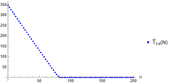
(a) T¯2a(N)=T(t;40,0,1000,N).\bar{T}_{2a}(N)=T(t^{*};40,0,1000,N).
Refer to caption
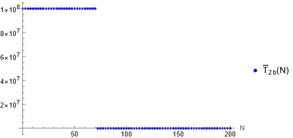
(b) T¯2b(N)=T(t;40,0,1000,N).\bar{T}_{2b}(N)=T(t^{**};40,0,1000,N).
Refer to caption
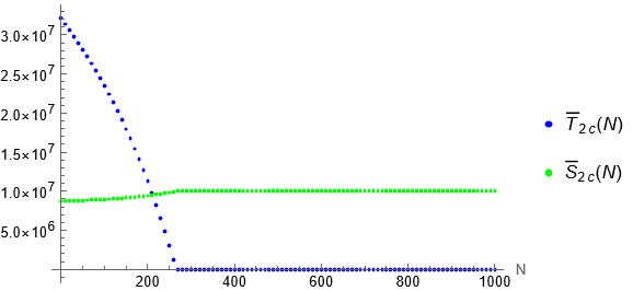
(c) T¯2c(N)=T(t;40,1,1000,N),\bar{T}_{2c}(N)=T(t^{*};40,1,1000,N), S¯2c(N):=S(t;40,1,1000,N).\bar{S}_{2c}(N):=S(t^{*};40,1,1000,N).
Refer to caption
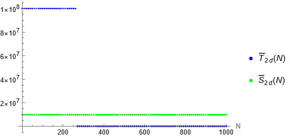
(d) T¯2d(N)=T(t;40,1,1000,N),\bar{T}_{2d}(N)=T(t^{**};40,1,1000,N), S¯2d(N):=S(t;40,1,1000,N).\bar{S}_{2d}(N):=S(t^{**};40,1,1000,N).
Refer to caption
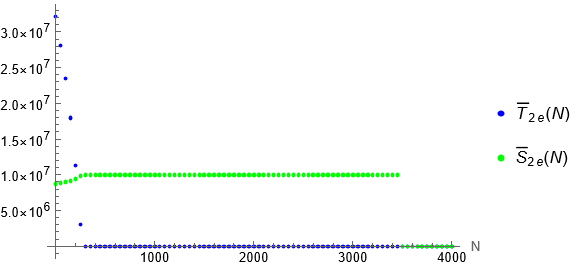
(e) T¯2e(N)=T(t;40,1,1000,N),\bar{T}_{2e}(N)=T(t^{*};40,1,1000,N), S¯2e(N):=S(t;40,1,1000,N).\bar{S}_{2e}(N):=S(t^{*};40,1,1000,N).
Refer to caption
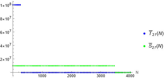
(f) T¯2f(N)=T(t;40,1,1000,N),\bar{T}_{2f}(N)=T(t^{**};40,1,1000,N), S¯2f(N):=S(t;40,1,1000,N).\bar{S}_{2f}(N):=S(t^{**};40,1,1000,N).
Figure 4: Plots of the values of solutions for small initial cancer cell populations after a given time depending on N.

The above inequalities are satisfied, in particular, for NN greater than approximately 1734.16.1734.16. Of course, for some initial conditions, lower values of NN may be sufficient to bring the number of cancer cells to 0. Figure 4(a) shows that for T0=40,S0=0,x0=1000T_{0}=40,S_{0}=0,x_{0}=1000 even N80N\approx 80 makes the number of cancer cells close to 0 after 33 months of treatment, while N60N\approx 60 is able to achieve the same goal after 33 years of treatment; see Fig. 4(b). Note that if the treatment administered is not strong enough to make the cancer cell population converge to 0 in 33 months, then the number of cancer cells will still grow to reach maximum capacity, although slower.

The situation changes dramatically when we introduce even a single cancer stem cell into the system, while leaving T0T_{0} and x0x_{0} unchanged. In fact, for T0=40,S0=1,x0=1000T_{0}=40,S_{0}=1,x_{0}=1000 the value of NN greater than 220220 is necessary to make the number of ordinary cancer cells close to 0 after 3 months of treatment, see Fig. 4(c). Figure 4(d) shows that the value of NN necessary to achieve the same goal after 33 years of treatment remains essentially the same. On the other hand, much stronger immunotherapy, NN larger than approximately 3500,3500, is required to make the number of cancer stem cells converge to 0,0, see Figs. 4(e)4(f).

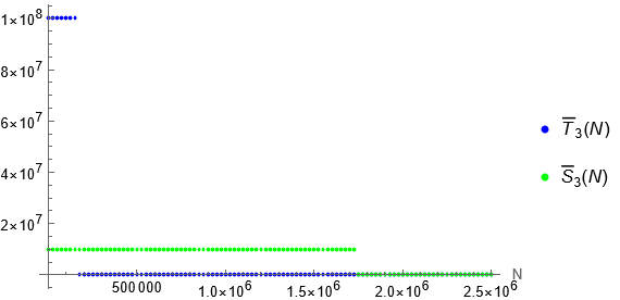
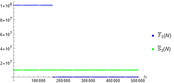
Figure 5 shows that the situation is not qualitatively different for slightly larger initial conditions – the value of NN that makes the number of CSCs converge to 0 in 33 years is more than ten times larger than the value of NN sufficient to achieve the same goal for ordinary cancer cells.

In Corollary 18 we state conditions on NN which guarantee that there is no strictly positive steady state exists, i.e. if the condition from the Corollary 18 is met, then there is no such steady state where cancer cell populations of both types survive. For our specific parameter values these conditions read

GT(N)rT(gx+ax,TKT+ax,SKS+μx)(KT+1)aT,xgx+μx1.464105,GS(N)rS(gx+ax,TKT+ax,SKS+μx)(KS+1)aS,xgx+μx1.464106.\begin{gathered}G_{T}(N)\geqslant\frac{r_{T}(g_{x}+a_{x,T}K_{T}+a_{x,S}K_{S}+\mu_{x})(K_{T}+1)}{a_{T,x}g_{x}+\mu_{x}}\approx 1.464\cdot 10^{5},\\ G_{S}(N)\geqslant\frac{r_{S}(g_{x}+a_{x,T}K_{T}+a_{x,S}K_{S}+\mu_{x})(K_{S}+1)}{a_{S,x}g_{x}+\mu_{x}}\approx 1.464\cdot 10^{6}.\end{gathered}

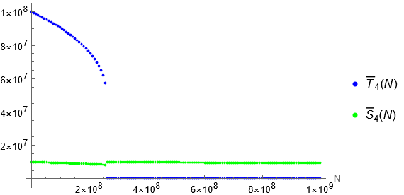
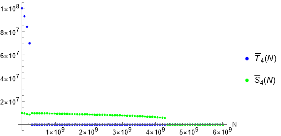
Inequalities above hold, in particular, for NN greater than approximately 1.75110101.751\cdot 10^{10}. Figure 6 seems to suggest that in fact much smaller NN is sufficient to eradicate all cancer cells even with maximal initial conditions T0=KT,S0=KS,x0=x(KT,KS).T_{0}=K_{T},S_{0}=K_{S},x_{0}=x^{*}(K_{T},K_{S}). Still, constant treatment of N4.2109,N\approx 4.2\cdot 10^{9}, which as per Fig. 6(b) appears to ensure full recovery after 33 months, may not be implementable in reality.
Refer to caption
(a)
Refer to caption
(b)
Figure 5: Plots of the values of solutions for larger initial cancer cell populations after a given time depending on N – T¯3(N)=T(t;2104,103,103,N),\bar{T}_{3}(N)=T(t^{**};2\cdot 10^{4},10^{3},10^{3},N), S¯3(N)=S(t;2104,103,103,N).\bar{S}_{3}(N)=S(t^{**};2\cdot 10^{4},10^{3},10^{3},N).
Refer to caption
(a)
Refer to caption
(b)
Figure 6: Plots of the values of solutions for maximal initial cancer cell populations after a given time depending on N – T¯4(N)=T(t;KT,KS,x(KT,KS),N),\bar{T}_{4}(N)=T(t^{**};K_{T},K_{S},x^{*}(K_{T},K_{S}),N), S¯4(N)=S(t;KT,KS,x(KT,KS),N).\bar{S}_{4}(N)=S(t^{**};K_{T},K_{S},x^{*}(K_{T},K_{S}),N).

4 Conclusion

In [9] Abernathy and Burke extended the GBM immunotherapy model proposed in [7] and further analyzed in [8], to account for the existence of CSCs. In this article, we applied a quasi-stationary approximation to this extended model, which yielded a simplified system with a reduced number of ODEs. We then introduced functions GTG_{T} and GSG_{S} that reflect the influence of immunotherapy on the dynamics of tumor cells and CSCs, respectively. We analyze the properties of these functions and show that they are strictly increasing, unbounded from above, and that GTG_{T} is greater than GSG_{S} for all positive values of NN (the total number of lymphocytes in the system at any given time), i.e. that the treatment has a stronger impact on tumor cells than CSC.

We then proceeded to analyze existence and local asymptotic stability of two types of steady states – the cure state (when no cancer cells survive the treatment) and the coexistence steady state (when some populations of both types of cancer cells survive) – depending on NN. In particular, we found sufficient conditions for the local asymptotic stability of the cure state and for the non-existence of the coexistence steady state. Finally, we illustrated our findings with numerical simulations performed for particular values of parameters appearing in the model.

A natural continuation of this work would be to relax the assumption that the therapy is constant in time and instead consider a treatment in the form of periodic impulses.

References

  • [1] Q.T. Ostrom, H. Gittleman, P. Farah, A. Ondracek, Y. Chen, Y. Wolinsky, N.E. Stroup, C. Kruchko, J.S. Barnholtz-Sloan. CBTRUS Statistical Report: Primary Brain and Central Nervous System Tumors Diagnosed in the United States in 2006-2010, Neuro-Oncology, 2013, 15(suppl 2), ii1–ii56.
  • [2] A. Becker, B. Sells, S. Haque, A. Chakravarti. Tumor Heterogeneity in Glioblastomas: From Light Microscopy to Molecular Pathology, Cancers, 2021, 13(4), 761.
  • [3] B.T. Himes, P.A. Geiger, K. Ayasoufi, A.G. Bhargav, D.A. Brown, I.F. Parney. Immunosuppression in Glioblastoma: Current Understanding and Therapeutic Implications, Frontiers in Oncology, 2021,11.
  • [4] Jigisha P. Thakkar and Therese A. Dolecek and Craig Horbinski and Quinn T. Ostrom and Donita D. Lightner and Jill S. Barnholtz-Sloan and John L. Villano. Epidemiologic and Molecular Prognostic Review of Glioblastoma, Cancer Epidemiology, Biomarkers & Prevention, 2014, 23(10), 1985–1996.
  • [5] C. Fernandes, A. Costa, L. Osório, R.C. Lago, P. Linhares, B. Carvalho, C. Caeiro. Current Standards of Care in Glioblastoma Therapy, in Glioblastoma, 197–241, Codon Publications, 2017.
  • [6] N. Desbaillets, A.F. Hottinger. Immunotherapy in Glioblastoma: A Clinical Perspective, Cancers, 2021, 13(15), 3721.
  • [7] N. Kronik, Y. Kogan, V. Vainstein, Z. Agur. Improving alloreactive CTL immunotherapy for malignant gliomas using a simulation model of their interactive dynamics, Cancer Immunology, Immunotherapy, 2007, 57(3), 425–439.
  • [8] Y. Kogan, U. Foryś, O. Shukron, N. Kronik, Z. Agur. Cellular immunotherapy for high grade gliomas: mathematical analysis deriving efficacious infusion rates based on patient requirements, SIAM Journal on Applied Mathematics, 2010, 70(6), 1953–1976.
  • [9] K. Abernathy, J. Burke. Modeling the Treatment of Glioblastoma Multiforme and Cancer Stem Cells with Ordinary Differential Equations, Computational and Mathematical Methods in Medicine, 2016, ID 1239861.
  • [10] B.T. Tan, C.Y. Park, L.E. Ailles, I.L. Weissman. The cancer stem cell hypothesis: a work in progress, Laboratory Investigation, 2006, 86(12), 1203–1207.