GCC: Generative Color Constancy via Diffusing a Color Checker

Abstract

Color constancy methods often struggle to generalize across different camera sensors due to varying spectral sensitivities. We present GCC, which leverages diffusion models to inpaint color checkers into images for illumination estimation. Our key innovations include (1) a single-step deterministic inference approach that inpaints color checkers reflecting scene illumination, (2) a Laplacian composition technique that preserves checker structure while allowing illumination-dependent color adaptation, and (3) a mask-based data augmentation strategy for handling imprecise color checker annotations. GCC demonstrates superior robustness in cross-camera scenarios, achieving state-of-the-art worst-25% error rates of 5.15° and 4.32° in bi-directional evaluations. These results highlight our method’s stability and generalization capability across different camera characteristics without requiring sensor-specific training, making it a versatile solution for real-world applications.

1 Introduction

Color constancy is a crucial aspect of computer vision, focused on determining the illumination of a scene to ensure that colors are accurately represented under varying lighting conditions. This process is essential for maintaining a consistent color appearance and for applications ranging from photography to autonomous driving. Traditional methods for color constancy, such as the Gray World [12], Gray Edge [58], and Shades-of-Gray [23] algorithms, rely on statistical assumptions about scene color distributions. While these methods are computationally efficient, they often struggle in challenging scenes with ambiguous color distributions[50]. More sophisticated statistical approaches, like Bright Pixels [38] and Gray Index [50], have been proposed but remain sensitive to violations of their underlying assumptions.

In contrast, learning-based methods have demonstrated superior performance by leveraging training data to learn complex illumination priors. Early approaches focused on gamut mapping [6, 15] or simple regression models [24]. With the advent of machine learning, methods such as Cheng Color Constancy (CCC) [17] employed regression-based learning, while Fast Fourier Color Constancy (FFCC) [9] utilized frequency-domain transformations to efficiently estimate illumination. Deep learning further advanced the field, with methods like C4 [8] and FC4 [37], the latter introducing confidence-weighted pooling to automatically identify important spatial regions for illumination estimation. However, a significant challenge in learning-based color constancy is that models are often constrained to specific camera sensors due to variations in spectral sensitivities [1, 27]. Models trained on one camera frequently fail to generalize to others without retraining or calibration [43].

Recent works have approached this problem from various angles. For instance, IGTN [63] introduced metric learning to learn scene-independent illuminant features, while quasi-unsupervised approaches [10] leverage semantic features of achromatic objects for better cross-sensor generalization. Several studies have attempted to address the multi-sensor challenge through domain adaptation techniques [20, 55] or by learning device-independent intermediate representations [1]. C5 [2] proposed an innovative approach that uses multiple unlabeled images from the target camera during inference to calibrate the model to new sensors. CLCC [45] further improved upon this by introducing contrastive learning to ensure that images of the same scene under different illuminants have distinct representations, while different scenes under the same illuminant have similar representations.

In this paper, we present a novel approach to color constancy that leverages inpainting techniques to integrate a color checker directly into the image. Our method utilizes Laplacian decomposition, allowing us to preserve high-frequency structural details while reducing the influence of low-frequency color information from the inserted color checker. In summary, we make the following contributions:

• We are the first to utilize inpainting for color checker integration in color constancy tasks, providing a new avenue for illumination estimation without the need for extensive camera-specific training data.

• By employing Laplacian decomposition, we enhance the model’s ability to generate a color checker that is structurally consistent with the input image, thereby improving the accuracy of color extraction from the patches.

• Our method operates in a deterministic manner, avoiding the introduction of noise during training and inference, which enables more reliable results with better computational efficiency.

2 Related Work

2.1 Color Constancy and White Balance

Color constancy research spans statistical-based and learning-based approaches. Statistical methods like Gray World [12], Gray Edge [58], Shades-of-Gray [23], Bright Pixels [38], and Gray Index [50] make assumptions about scene color statistics but struggle with challenging scenes. Learning-based methods have proven more effective, evolving from gamut mapping [6, 15] and regression models [24] to deep learning approaches. Notable developments include CCC [8], FFCC [9], and FC4 [37]. A key challenge is camera-specific spectral sensitivity [1, 27], requiring retraining or calibration for new sensors [43]. Recent solutions include IGTN’s [63] metric learning, quasi-unsupervised learning [10], and domain adaptation approaches [20, 55]. C5 [2] uses unlabeled target camera images during inference, while CLCC [45] employs contrastive learning to improve feature representations. Our work leverages diffusion models for color checker inpainting, offering a novel approach to illumination estimation without extensive camera-specific training data.

2.2 Image-Conditional Diffusion Models

Denoising Diffusion Probabilistic Models (DDPMs) [57] achieve state-of-the-art generation by reversing a noising process with UNet architectures [53], demonstrating excellence in density estimation and sample quality [41, 22]. Latent Diffusion Models (LDMs) [52] improved efficiency by operating in compressed latent space and introduced cross-attention conditioning. This enabled powerful inpainting capabilities, demonstrated by Blended Diffusion [4, 5], Paint-by-Example [64], ControlNet [69], and IP-Adapter [66]. Recent work identified that perceived limitations were often due to DDIM scheduler implementation issues [44] rather than fundamental constraints. Our work leverages these insights to effectively adapt diffusion models for color checker inpainting in illumination estimation.

2.3 Learning-based Lighting Estimation

Lighting estimation methods traditionally use physical probes like mirror balls [21], 3D objects [62, 46], eyes [48], or faces [13, 67]. Early probe-free approaches used limited models like directional lights [39], sky models [35, 34], or spherical harmonics [30]. Modern methods focus on HDR environment maps, pioneered by Gardner et al. [29]. DeepLight [42] and EverLight [19] handle both indoor and outdoor scenes, while StyleLight [61] uses GANs for joint LDR-HDR prediction. Some works explore panorama outpainting [3, 18] but struggle with HDR [19]. Recently, DiffusionLight [49] introduced virtual chrome ball synthesis using diffusion models. Our work follows a similar direction but focuses on color checker inpainting for illumination estimation.

2.4 Fine-tuning Strategies for Diffusion Models

For personalization, DreamBooth [54] pioneered special token fine-tuning, while Gal et al. [25] and Voynov et al. [60] proposed learned word embeddings approaches. For geometry estimation, Marigold [40] demonstrated successful fine-tuning using synthetic data. Garcia et al. [28] revealed that simple end-to-end fine-tuning can outperform complex approaches once DDIM implementation issues are fixed. For efficiency, LoRA [36] introduced low-rank weight changes, while SVDiff [33] and orthogonal fine-tuning [51] proposed alternative parameterizations. Following Garcia et al. [28], we adopt simple full fine-tuning strategies for our color checker inpainting task.

3 Method

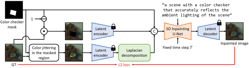
Figure 2: Overview of our training pipeline. Starting from pretrained stable-diffusion-2-inpainting, we enable color checker generation through end-to-end fine-tuning. Given a ground truth color checker image and its mask, we apply color jittering in the masked region. The input image latent passes through Laplacian composition before being concatenated with the masked image latent and the resized mask for the SD Inpainting U-Net. The model is trained with an L2 loss between the inpainted output and ground truth image at a fixed timestep $T$.

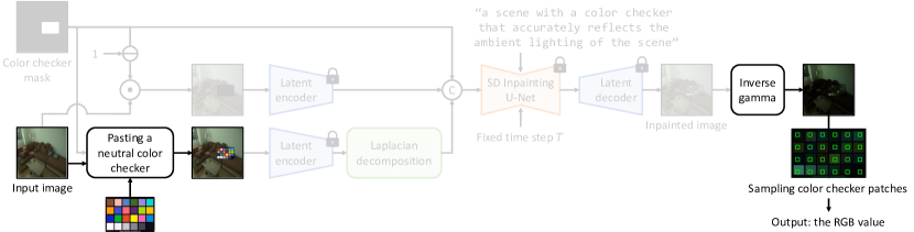
Figure 3: Overview of our inference pipeline for illumination estimation. A neutral color checker is pasted onto the input image, which is then encoded into the latent space. The input latent is processed through Laplacian composition before being concatenated with the masked image latent and the resized mask. The modified U-Net generates an inpainted result at fixed timestep $T$. After inverse gamma correction, we sample the color checker patches to obtain the final RGB illumination value. We highlight the steps and components that are different from the training pipeline.

Instead of directly predicting environmental RGB light, we propose to leverage diffusion models’ rich priors to inpaint a color checker into the scene and extract illumination colors from it. As shown in Figs. 2 and 3, our pipeline consists of (1) During training, we fine-tune a diffusion-based inpainting model at timestep t=T with images containing color checkers, optimizing for deterministic single-step inference (Sec. 3.1-3.2). (2) We introduce Laplacian decomposition to maintain the checker’s high-frequency structure while allowing illumination-aware color adaptation (Sec. 3.3). (3) At inference time, we composite a neutral color checker into a given scene and use our fine-tuned model to inpaint it according to the scene illumination, from which we extract environmental colors (Sec. 3.4).

3.1 Network Architecture

We base our model on stable-diffusion-2-inpainting [52] for its specialized local editing capability. The model consists of a VAE encoder-decoder pair ($\mathcal{E}$, $\mathcal{D}$) and a U-Net denoising backbone. Given an RGB image $I\in\mathbb{R}^{H\times W\times 3}$ and a binary mask $M\in\{0,1\}^{H\times W}$ indicating the color checker region, we first encode both the masked image and the original image into the latent space as $z_{\text{masked}}=\mathcal{E}(I\odot(1-M))$ and $z=\mathcal{E}(I)$, where $\odot$ denotes element-wise multiplication. The mask $M$ is downscaled by a factor of 8 to match the latent resolution as $M^{\prime}\in\mathbb{R}^{h\times w}$, where $h=H/8,w=W/8$. During training, the U-Net denoiser $\epsilon_{\theta}$ takes as input the concatenation of the noised latent $z_{t}$, the downscaled mask $M^{\prime}$, and the masked image latent $z_{\text{masked}}$ along the channel dimension as $z_{\text{combined}}=[z_{t},M^{\prime},z_{\text{masked}}]\in\mathbb{R}^{h\times w\times(2d+1)}$, where $d$ is the latent dimension. Together with the timestep $t$ and text embedding $c$, the denoiser is trained to predict the noise as $\epsilon_{\theta}(z_{\text{combined}},t,c)\rightarrow\mathbb{R}^{h\times w\times d}$. At inference time, we obtain the final inpainted result by decoding the denoised latent $\hat{I}=\mathcal{D}(z_{0})$, where only the color checker region is modified while leaving the rest unmodified, making this architecture particularly suitable for color constancy task.

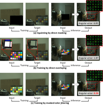
Figure 4: Analysis of color checker alignment strategies. (a) Direct inpainting on masked regions leads to poor color checker structure. This is because we do not provide any guidance on the desired color checker structure, causing the model to generate contours that do not meet our expectations. (b) Using a homography transform to overlay a template suffers from pixel-level misalignment due to imprecise bounding box annotations. (c) Our mask color jittering approach overcomes corner point annotation limitations by allowing the model generate geometrically consistent color checker structures while accurately reflecting scene illumination.

3.2 End-to-End Fine-Tuning

Training.

Although pre-trained diffusion models like SD and SD inpainting [52] models have been exposed to diverse image collections, additional fine-tuning crucial for generating precise color checkers that accurately reflect environmental illumination. As shown in our experiments Fig. 6, fine-tuning significantly impacts the model’s ability to generate color checkers that faithfully represent scene illumination.

Although SDEdit [47] could be applied to our task, it faces a fundamental trade-off in noise level selection. On one hand, insufficient noise fails to effectively suppress the original chromatic information from the input image, making it difficult to adapt to the target scene illumination. On the other hand, excessive noise, while better at removing unwanted color information, can disrupt the structural consistency between the generated result and the input reference. Furthermore, for color constancy tasks, maintaining a one-to-one correspondence between input and output is essential. While traditional diffusion models’ stochastic nature allows for ensemble improvements through multiple inferences, this comes at increased computational cost.

Following [28], we adopt an end-to-end fine-tuning approach that enables single-step deterministic inference while maintaining high-quality color checker generation. Specifically, we fine-tune the inpainting U-Net at a fixed timestep $t=T$ as shown in Fig. 2.

Given an input image $I$ and its corresponding mask $\mathbf{M}$, we first obtain the augmented image $I_{\text{aug}}$ by applying color jittering to the masked region. We then obtain its latent representation through the VAE encoder, $\mathbf{z}^{*}=\mathcal{E}(I_{\text{aug}})$. The latent representation is processed through Laplacian decomposition to extract high-frequency components, $\mathbf{z}_{h}=\mathcal{H}(\mathbf{z}^{*})$. For single-step prediction, we directly set the noise term $\boldsymbol{\epsilon}=\mathbf{0}$ in the forward process: $\mathbf{z}_{T}=\sqrt{\bar{\alpha}_{T}}\mathbf{z}_{h}+\sqrt{1-\bar{\alpha}_{T}}\boldsymbol{\epsilon}$. The denoised latent is then obtained through $\hat{\mathbf{z}}_{0}=\sqrt{\bar{\alpha}_{T}}\mathbf{z}_{T}-\sqrt{1-\bar{\alpha}_{T}}\epsilon_{\theta}(\mathbf{z}_{\text{combined}},T,c)$, where $\mathbf{z}_{\text{combined}}=[\mathbf{z}_{T},\mathbf{M}^{\prime},\mathbf{z}_{\text{masked}}]\in\mathbb{R}^{h\times w\times(2d+1)}$ represents the concatenated input features along the channel dimension, and $c$ denotes the text condition. Finally, we decode the latent to obtain the inpainted image: $\hat{I}=\mathcal{D}(\hat{\mathbf{z}}_{0})$. The model is optimized using a mean squared error loss:

$$\mathcal{L}=\frac{1}{HW}\sum_{i,j}(I^{*}_{i,j}-\hat{I}_{i,j})^{2},$$ (1)

where $(i,j)$ denotes the pixel coordinates, and $H$ and $W$ are the height and width of the image, respectively.

Color checker misalignment issue.

Existing color constancy datasets [16, 31] only provide rough bounding boxes for color checkers instead of precise corner point locations. This hinders our ability to accurately align the standard sRGB color checker with the one in the original image, affecting the model’s learning of the transformation from standard to harmonized colors. To overcome this limitation, we designed a mask region-based data augmentation method.

We first analyze two intuitive solutions: directly masking and allowing the model to perform inpainting. This approach results in generated color checkers with contours that do not meet our expectations, making accurate color extraction from the patches difficult (Fig. 4 (a)). The second solution involved overlaying the color checker template directly onto the original image (Fig. 4 (b)). However, due to the absence of precise corner point locations, alignment with the raw checker remains imperfect at a per-pixel level even using homography transform.

Masked color jittering.

Therefore, we further explored a third approach: directly applying strong color jittering to the mask region (Fig. 4 (c)). This seemingly counterintuitive method aims to destroy clues that may leak sensor-specific information, forcing the model to rely on information outside the mask region to reconstruct the original color checker that aligns with the ground truth.

Random color jittering to the masked color checker region helps our model learn a more robust mapping between the standard and scene-specific color spaces. The augmented image $\hat{I}$ is obtained by:

$$I_{\text{aug}}=(1-M)\odot I+M\odot\mathcal{T}(I),$$ (2)

where $I$ is the input image, $M$ is the binary mask, $\odot$ denotes element-wise multiplication, and $\mathcal{T}(\cdot)$ represents the color jittering function that randomly applies brightness, contrast, saturation adjustments and Gaussian noise to the masked region. By randomly perturbing the color checker region, we force the model to rely on contextual illumination cues rather than local color checker patterns. This approach overcomes the limitations of imprecise annotations in existing datasets and enhances the model’s ability to learn accurate illumination estimation from scene context.

3.3 Laplacian Decomposition

Although mask color jittering addresses the imprecise corner annotation issue, the randomness in jittering may occasionally allow low-frequency information leakage from the masked region. This could cause the model to simply reconstruct the masked area rather than harmonize it with the scene illumination. To address this issue, we introduce the Laplacian decomposition technique.

By extracting only the high-frequency components of the input image through Laplacian decomposition, our approach serves two purposes: First, it preserves the structural details needed to generate a color checker that faithfully maintains the patch layout of our pre-pasted reference. Second, it minimizes the influence of low-frequency color information, encouraging the model to focus on harmonizing the generated color checker with the scene illumination rather than reconstructing the original colors.

The detailed Laplacian decomposition process is presented in Algorithm 1. The key benefit of Laplacian decomposition, as shown in Fig. 6, allows the model to generate color checkers that maintain structural consistency while correctly reflecting scene illumination, enabling accurate illumination estimation.

Input: Input latent $z\in\mathbb{R}^{B\times C\times H\times W}$, pyramid levels $L$

Output: High-frequency components $z_{h}$

Initialize $z_{h}=0$

$k\leftarrow$ 3×3 Gaussian kernel

for each channel $c$ in $C$ do

    $z_{\text{curr}}\leftarrow z[c]$

     // Current level features

    for $l=0$ to $L-1$ do

       $z_{\text{blur}}\leftarrow k*z_{\text{curr}}$

        // Gaussian blur

       $z_{\text{high}}\leftarrow z_{\text{curr}}-z_{\text{blur}}$

        // High-freq details

       if $l=0$ then

          $z_{h}[c]\leftarrow z_{\text{high}}$

      else

          $z_{h}[c]\leftarrow z_{h}[c]+\texttt{Upsample}(z_{\text{high}})$

       end if

      $z_{\text{curr}}\leftarrow\texttt{AvgPool}(z_{\text{blur}})$

        // Downsample

      

    end for

   

end for

return $z_{h}$

Algorithm 1 High-frequency Extraction via Laplacian Pyramid

3.4 Inference

The complete inference pipeline of our method is illustrated in Fig. 3, which consists of the following steps:

Color checker generation.

We first composite a fixed-size neutral color checker centered at the mask region. The input image is then gamma-corrected with $\gamma=2.2$ to transform it to the sRGB domain. This preprocessed image is processed through our model in a single forward pass with fixed timestep $t=T$. The output is then inverse gamma-corrected to obtain the raw domain result.

Illumination estimation.

Since we have precise control over the initial color checker placement and the Laplacian decomposition ensures structural preservation, we can reliably extract color information from each patch. Specifically, we apply perspective transformation to align the generated checker into a standardized rectangular grid, followed by applying fixed grid masks to sample colors from each patch. The scene illumination is then estimated from the achromatic patches of the color checker.

4 Experiments

4.1 Experimental Setup

Dataset.

We use two publicly available color constancy benchmark datasets in our experiments: the NUS 8-Camera dataset [16] and the re-processed Color Checker dataset [31] (referred to as the Gehler dataset). The Gehler dataset contains 568 original images captured by two different cameras, while the NUS 8-Camera dataset [16] contains 1736 original images captured by eight different cameras. Each image in both datasets includes a Macbeth Color Checker (MCC) chart, which serves as a reference for the ground-truth illuminant color.

For both datasets, we adopt a three-fold cross-validation protocol for our experimental evaluation. This ensures that the training and testing data are completely separated, reflecting the model’s generalization capability to unseen scenarios.

Since the pre-trained VAE was trained on sRGB images, we apply a gamma correction of $\gamma=1/2.2$ on linear RGB images before encoding to minimize the domain gap. Conversely, after VAE decoding, we apply inverse gamma correction to convert the output back to the linear domain for metric evaluation.

Evaluation metrics.

To evaluate the performance of color constancy methods, we use the standard angular error metric, which measures the angular difference between the estimated illuminant and the ground-truth illuminant. Specifically, the angular error $\theta$ between an estimated illuminant vector $\hat{\mathbf{y}}$ and the ground-truth illuminant vector $\mathbf{y}$ is defined as:

$$\theta=\arccos\left(\frac{\hat{\mathbf{y}}\cdot\mathbf{y}}{|\hat{\mathbf{y}}||\mathbf{y}|}\right)$$ (3)

The angular error is measured in degrees, with smaller values indicating better estimation accuracy. Following previous works, we report the following statistics of the angular error.

4.2 Implementation Details

Our implementation is based on the Stable Diffusion v2 framework [52] using PyTorch, following parameter settings from [28]. We train our models using the Adam optimizer with an initial learning rate of $5\times 10^{-5}$ and apply exponential learning rate decay after a 150-step warm-up period.

For cross-validation experiments, we train for 6k iterations with batch size 4 on the NUS-8 dataset, and 13k iterations with batch size 8 on the Gehler dataset. For cross-dataset evaluation, when training on the Gehler dataset and testing on NUS-8, we use a batch size of 8 with no gradient accumulation for 12k iterations. When training on NUS-8 and testing on the Gehler dataset, we use a batch size of 8 with gradient accumulation over 2 steps (effective batch size of 16) for 15k iterations.

For data augmentation, we follow FC4 [37] to rescale images by random RGB values in [0.6, 1.4], noting that we only rescale the input images since our training does not require ground truth illumination. The rescaling is performed in the raw domain, followed by gamma correction. This is implemented through a 3×3 color transformation matrix, where diagonal elements control the intensity of individual RGB channels (color strength), and off-diagonal elements determine the degree of color mixing between channels (color offdiag). With a probability of 0.8, we randomly crop a region containing the mask, where the crop size ranges from 80% to 100% of the original image dimensions while ensuring the mask remains fully visible. Additionally, we apply local transformations to masked regions only, including brightness adjustment ($[0.8,2.0]$), saturation adjustment ($[0.8,1.3]$), contrast adjustment ($[0.8,1.3]$), and Gaussian noise ($\sigma\in[0,30]$).

For the Laplacian decomposition, we use a two-level pyramid ($L=2$) to balance the preservation of high-frequency structural details and the suppression of low-frequency color information.

All experiments were conducted on an NVIDIA RTX 4090 GPU. We will make our source code and fine-tuned model weights publicly available for reproducibility.

Table 1: Camera-agnostic evaluation. All results are in units of degrees.

Training set	NUS 8-Camera [17]					Color Checker [56]
Testing set	Color Checker [56]					NUS 8-Camera [17]
Method	Mean	Median	Tri-mean	Best 25%	Worst 25%	Mean	Median	Tri-mean	Best 25%	Worst 25%
Statistical Methods
White-Path [11]	7.55	5.68	6.35	1.45	16.12	9.91	7.44	8.78	1.44	21.27
Gray-World [12]	6.36	6.28	6.28	2.33	10.58	4.59	3.46	3.81	1.16	9.85
1st-order Gray-Edge [59]	5.33	4.52	4.73	1.86	10.43	3.35	2.58	2.76	0.79	7.18
2nd-order Gray-Edge [59]	5.13	4.44	4.62	2.11	9.26	3.36	2.70	2.80	0.89	7.14
Shades-of-Gray [23]	4.93	4.01	4.23	1.14	10.20	3.67	2.94	3.03	0.99	7.75
General Gray-World [7]	4.66	3.48	3.81	1.00	10.09	3.20	2.56	2.68	0.85	6.68
Grey Pixel (edge) [65]	4.60	3.10	-	-	-	3.15	2.20	-	-	-
Cheng et al. [17]	3.52	2.14	2.47	0.50	8.74	2.92	2.04	2.24	0.62	6.61
LSRS [26]	3.31	2.80	2.87	1.14	6.39	3.45	2.51	2.70	0.98	7.32
GI [50]	3.07	1.87	2.16	0.43	7.62	2.91	1.97	2.13	0.56	6.67
Learning-based Methods
Bayesian [32]	4.75	3.11	3.50	1.04	11.28	3.65	3.08	3.16	1.03	7.33
Chakrabarti [14]	3.52	2.71	2.80	0.86	7.72	3.89	3.10	3.26	1.17	7.95
FFCC [9]	3.91	3.15	3.34	1.22	7.94	3.19	2.33	2.52	0.84	7.01
SqueezeNet-FC4 [37]	3.02	2.36	2.50	0.81	6.36	2.40	2.03	2.10	0.70	4.80
C${}^{4}_{\text{SqueezeNet-FC4}}$ [68]	2.73	2.20	2.28	0.72	5.69	2.28	1.90	1.97	0.67	4.60
SIIE [1]	3.72	2.46	2.79	1.02	8.51	4.24	3.88	3.93	1.45	7.66
CLCC [45]	3.05	2.44	2.51	0.89	6.30	3.42	2.95	3.06	0.94	6.70
C5 [2]	3.34	2.57	2.68	0.78	7.39	2.65	1.98	2.14	0.66	5.72
Ours	2.62	2.19	2.29	0.88	5.15	2.35	2.06	2.12	0.87	4.32

4.3 Results and Comparisons

For evaluation, we follow the standard protocol of three-fold cross-validation on both the NUS-8 Camera dataset [16] and the re-processed Color Checker dataset [31]. Due to space limitations, we present the complete cross-validation results in the supplementary material.

As shown in Tab. 1, our method demonstrates superior robustness in cross-dataset evaluation, where we train on one dataset and test on another. In this challenging scenario, our method achieves state-of-the-art performance particularly in the worst-25% metric, obtaining 5.22 degrees when trained on NUS-8 and tested on Gehler, and 4.32 degrees in the reverse setting. This improvement in handling difficult cases demonstrates the stability and generalization capability of our approach, suggesting that our method effectively leverages the pretrained diffusion prior to learn robust illumination patterns.

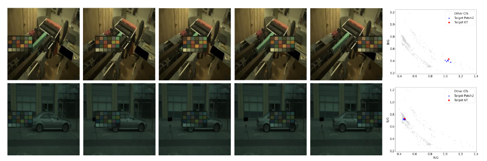
Figure 5: Sensitivity to color checker placement. This figure demonstrates the robustness of our method across various color checker positions in the scene. The left part displays different placements of color checkers and their corresponding processed results, showing that our method remains effective under challenging warm color temperatures (regions with lower data distribution). The scatter plots on the right quantitatively validate this observation, where the estimated illumination values consistently cluster near the ground truth target, confirming the precision and consistency of our approach.

Fig. 5 demonstrates the robustness and novel capabilities of our proposed method compared to prior approaches. In contrast to prior approaches, our method’s ability to perform sampling at different positions and generate result ensembles allows us to quantify model uncertainty, showcasing the precision and consistency of our approach.

Despite utilizing diffusion model, our method maintains efficient inference times due to its single-step design. Using an NVIDIA RTX 4090 GPU, our method processes a 512$\times$512 image in 180ms, making it practical for real-world applications. This is significantly faster than traditional diffusion-based methods that typically require multiple denoising steps, as shown in Tab. 2 while maintaining diffusion priors’ benefits for accurate color constancy estimation.

4.4 Ablation Studies

We conducted a series of ablation experiments to validate the importance of key design choices, including using Laplacian composition, noise prediction-based LoRA fine-tuning, and mask-based data augmentation in Tab. 3.

Table 2: Comparison between fine-tuned SDXL inpainting and our one-step model. All metrics are reported in degrees, and inference time is measured on a single 512$\times$512 image using an NVIDIA RTX 4090 GPU. All models are trained on the NUS-8 Camera dataset [17] and evaluated on the re-processed Color Checker dataset [31].

Method	Steps	Ensemble	Inference	Metrics (∘)
			time (s)	Mean	Median	Best-25%	Worst-25%
SDXL Inpainting (SDEdit)	25	10	17.98	4.47	3.25	1.07	10.01
Full Model	1	1	0.18	2.62	2.19	0.88	5.15

Table 3: Ablation study on key components of our method. We evaluate the impact of different components: Laplacian composition (Lap.), color checker inpainting vs. direct RGB prediction, and masked color jittering (Mask DA). All models are trained on the NUS-8 Camera dataset [17] and evaluated on the re-processed Color Checker dataset [31]. The results show that our color checker inpainting approach outperforms direct RGB prediction, and the combination with other components (Laplacian composition, and masked color jittering) yields the best performance. All error metrics are reported in degrees, with lower values indicating better performance.

Noise	Lap.	Inpaint	Mask DA	Mean	Median	Best-25%	Worst-25%
Zeros	-	✓	✓	3.71	2.86	1.31	7.68
Zeros	✓	✓	-	3.52	2.76	1.25	6.78
Zeros	-	-	-	2.98	2.53	1.26	6.14
Zeros	✓	✓	✓	2.62	2.19	0.88	5.15

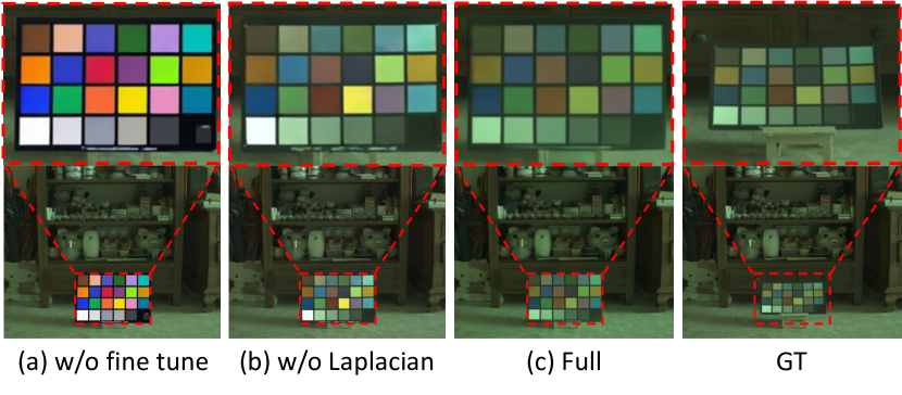
Figure 6: Importance of fine-tuning and Laplacian composition. (a) Results without fine-tuning show poor color checker quality due to the domain gap between pretrained diffusion model’s training data (sRGB images) and our gamma-corrected raw images, leading to disharmonious inpainting results. (b) Results without Laplacian composition are biased by the low-frequency information from the neutral color checker, leading to inharmonious generation. (c) Our full method with both components produces well-harmonized color checkers that accurately reflect scene illumination.

Without Laplacian decomposition.

In this experiment, we solely rely on the VAE encoder’s latent representation as model input without utilizing the high-frequency components from the Laplacian decomposition. As shown in  Fig. 6, the generated color checker is adversely affected by the low-frequency information from the neutral reference color checker initially placed in the scene. These disharmonious colors in the synthesized color checker lead to inaccurate color source estimation, as we can no longer extract reliable color values for computing the environment color.

With noise.

In this experiment, we used LoRA [36] to fine-tune the SDXL inpainting model. While the model architecture is the same as stable-diffusion-2-inpainting, we adopted a noise prediction-based training approach: we inject noise into the latent representation of the input image and train the model to predict this noise, optimizing the LoRA parameters by computing the L2 loss between the predicted and actual noise. During inference, we employ SDEdit with a noise strength of 0.6 and 25 denoising steps and compute the median from 10 generated samples. However, this approach shows limited effectiveness compared to our final method. The main limitation stems from the trade-off between maintaining the color checker’s geometry and suppressing the low-frequency information from the neutral color checker. While we need to preserve the color checker’s shape, the insufficient noise level fails to effectively suppress the low-frequency information from the neutral color checker, resulting in inferior color estimation.

Without mask data augmentation.

Initially, we use the color checker corner locations provided in the datasets and apply a homography matrix to align the standard color checker to the original position. However, the inaccuracy of corner detection leads to pixel alignment issues. To overcome this limitation, we employ the mask-based data augmentation approach, which avoids dependence on precise corner locations and effectively generates color checkers that harmonize with the scene. The reliance precise corner locations proves problematic, making our mask-based approach superior for generating scene coherent color checkers.

Without inpainting color checker.

In this experiment, we did not obtain the environment white balance color by inpainting a color checker. Instead, we directly let the diffusion model predict the final output RGB. This direct prediction approach proves less effective than our inpainting-based method, highlighting the importance of using color checker references for accurate environmental color estimation.

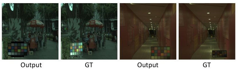
Figure 7: Failure cases. Our approach struggles when there is a significant mismatch between the illumination of the original color checker and the ambient lighting in the scene.

5 Conclusion

In this work, we have presented a novel approach to color constancy that leverages image-conditional diffusion models to inpaint color checkers directly into images. This method not only enhances the accuracy of illumination estimation but also addresses significant limitations of traditional techniques, particularly their struggles with generalization across different camera sensors. By employing Laplacian decomposition, we effectively preserve high frequency structural details, ensuring that the inpainted color checkers harmonize with the original image context.

Limitations.

As shown in Fig. 7, our method struggles when there is a significant mismatch between the inpainted color checker and the scene’s ambient lighting. This typically occurs in challenging scenarios with multiple strong light sources of different colors or complex spatially-varying illumination. While diffusion models provide strong image priors, they sometimes prioritize visual plausibility over physical accuracy, especially in extreme lighting conditions.

Overview

This supplementary material presents additional details and results to complement the main manuscript. In Section A, we provide comprehensive implementation details, including dataset preprocessing protocols and training configurations. Section B presents an empirical analysis of the impact of different pyramid levels in our Laplacian decomposition technique. Section C showcases qualitative results demonstrating our method’s effectiveness across various datasets and real-world scenarios, while Section D details our cross-validation evaluation protocol and comparative analysis with state-of-the-art methods. We will release our complete training and inference code along with pre-trained weights to facilitate future research in this area.

Appendix A Implementation Details

A.1 Datasets and Preprocessing

We use two publicly available color constancy benchmark datasets in our experiments: the NUS 8-Camera dataset [16] and the re-processed Color Checker dataset [31] (referred to as the Gehler dataset). The Gehler dataset contains 568 original images captured by two different cameras, while the NUS 8-Camera dataset [16] contains 1736 original images captured by eight different cameras. Each image in both datasets includes a Macbeth Color Checker (MCC) chart, which serves as a reference for the ground-truth illuminant color.

Following the evaluation protocol in [1], several standard metrics are reported in terms of angular error in degrees: mean, median, tri-mean of all the errors, the mean of the lowest 25% of errors, and the mean of the highest 25% of errors.

Following the preprocessing protocol from [37], we process the raw image data before applying gamma correction for sRGB space conversion.

Since the pre-trained VAE was trained on sRGB images, we apply a gamma correction of $\gamma=1/2.2$ on linear RGB images before encoding to minimize the domain gap. Conversely, after VAE decoding, we apply inverse gamma correction to convert the output back to the linear domain for metric evaluation.

A.2 Training Details

Full Model

We train our models using the Adam optimizer with an initial learning rate of $5\times 10^{-5}$ and apply exponential learning rate decay after a 150-step warm-up period. For cross-validation experiments, we train for 6k iterations with a batch size of 2 on the NUS-8 Camera dataset and 13k iterations with a batch size of 4 on the Gehler dataset. For cross-dataset evaluation, when training on the Gehler dataset and testing on NUS-8, we use a batch size of 8 with no gradient accumulation for 12k iterations. When training on NUS-8 and testing on the Gehler dataset, we use a batch size of 8 with gradient accumulation over 2 steps (effective batch size of 16) for 15k iterations.

SDXL Inpainting (SDEdit)

For the SDXL inpainting model [52] with LoRA fine-tuning experiments, we use a learning rate of $5\times 10^{-5}$ and a LoRA rank of 4. In the cross-dataset experiment from the NUS-8 Camera dataset to the Gehler dataset, we train for 20,000 iterations with batch size 4.

A.3 Inference Settings

Full Model

Following Garcia et al. [28], we employ DDIM scheduler with a fixed timestep $t=T$ and trailing strategy during inference for deterministic single-step generation. Our implementation is based on the stable-diffusion-2-inpainting model [52].

SDXL Inpainting (SDEdit)

For comparison, we also implement a version using SDXL inpainting model [52] with LoRA [36] fine-tuning. During inference, we use the DDIM scheduler with 25 denoising steps and SDEdit with a noise strength of 0.6, a guidance scale of 7.5, and a LoRA scale of 1. The final illumination estimation is obtained by computing the median from an ensemble of 10 generated samples.

Appendix B Laplacian Decomposition

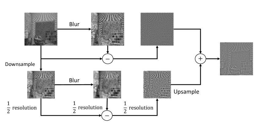
Figure 8: Flow diagram of Laplacian composition. Frequency component fusion through two-level ($1/2$ resolution) blur, downsample, and composition operations.

B.1 Laplacian Deomposition Visualization

In Fig. 8, we visualize how our Laplacian decomposition technique preserves high-frequency structural details while allowing illumination-dependent color adaptation. The pyramid decomposition effectively separates the color checker’s geometric pattern from its chromatic information, enabling our model to maintain structural consistency while accurately reflecting scene illumination.

B.2 Analysis of Pyramid Level Selection

We conduct experiments with different numbers of pyramid levels (L = 1,2,3) to analyze the effectiveness of our Laplacian composition. As shown in Tab. 4, using two-level decomposition (L = 2) achieves the best performance across all metrics. Adding more levels not only increases computational complexity but also leads to performance degradation, as the additional levels introduce more low-frequency information that can adversely affect the harmonious generation of color checkers.

Appendix C Additional Qualitative Results

C.1 Benchmark Datasets

On the NUS-8 Camera dataset and Gehler dataset, we utilize the original mask locations to place fixed-size neutral color checkers in our experiments. The results Fig. 9 and Fig. 10 demonstrate our method’s ability to generate structurally coherent color checkers that naturally blend with the scene while accurately reflecting local illumination conditions, enabling effective color cast removal across diverse lighting scenarios.

C.2 In-the-wild Images

For in-the-wild scenes, we adopt a center-aligned placement strategy to address camera vignetting effects, which can impact color accuracy near image edges. This consistent central positioning not only mitigates lens shading issues but also demonstrates our method’s flexibility in color checker placement. The results Fig. 11 validate our approach’s robustness in practical photography applications, showing consistent performance in white balance correction despite the fixed central placement strategy.

C.3 Interactive Visualization

We provide an interactive HTML interface that visualizes results with color checkers placed at different locations within scenes. The visualization demonstrates that our method produces accurate outputs with minimal variation across different placement positions. The results show that the estimated illumination values consistently cluster near the ground truth target regardless of the checker’s position, confirming our method’s reliability and position-independence in illumination estimation.

Appendix D Cross-validation Results

For evaluation, we follow the standard protocol of three-fold cross-validation on both the NUS-8 Camera dataset [16] and the Gehler dataset [31]. The results are presented in Tab. 5 and Tab. 6. As FC4 notes, many scenes have multiple light sources with differences up to 10 degrees, so further reducing an error already under 2 degrees may not be a strong comparison. Instead, our method inpaints physically plausible color checkers—a different strategy than directly optimizing for a ground truth illumination RGB, which can yield lower single-camera performance but enables strong cross-camera generalization, as shown in our cross-dataset experiments.

Table 4: Analysis of different pyramid levels in Laplacian composition. Results are trained on the NUS-8 Camera dataset and tested on Gehler dataset .

Level	Mean	Median	Best-25%	Worst-25%
L = 1	3.53	3.27	1.48	6.03
L = 2	2.67	2.25	0.89	5.22
L = 3	3.16	2.83	1.25	5.62

Table 5: Result on NUS-8 Camera dataset, with mean angular error in degrees.

NUS-8 Camera dataset	Mean	Med.	Tri.	Best	Worst
				25%	25%
CCC [8]	2.38	1.48	1.69	0.45	5.85
AlexNet-FC4 [37]	2.12	1.53	1.67	0.48	4.78
FFCC [9]	1.99	1.31	1.43	0.35	4.75
C${}^{4}_{\text{SqueezeNet-FC4}}$ [68]	1.96	1.42	1.53	0.48	4.40
CLCC [45]	1.84	1.31	1.42	0.41	4.20
Ours	2.10	1.52	1.69	0.56	4.38

Table 6: Result on Gehler dataset, with mean angular error in degrees.

Gehler dataset	Mean	Med.	Tri.	Best	Worst
				25%	25%
CCC [8]	1.95	1.22	1.38	0.35	4.76
SqueezeNet-FC4 [37]	1.65	1.18	1.27	0.38	3.78
FFCC [9]	1.61	0.86	1.02	0.23	4.27
C${}^{4}_{\text{SqueezeNet-FC4}}$ [68]	1.35	0.88	0.99	0.28	3.21
CLCC[45]	1.44	0.92	1.04	0.27	3.48
Ours	1.91	1.80	1.84	0.60	3.46

Figure 9: Qualitative results for the NUS-8 Camera dataset.

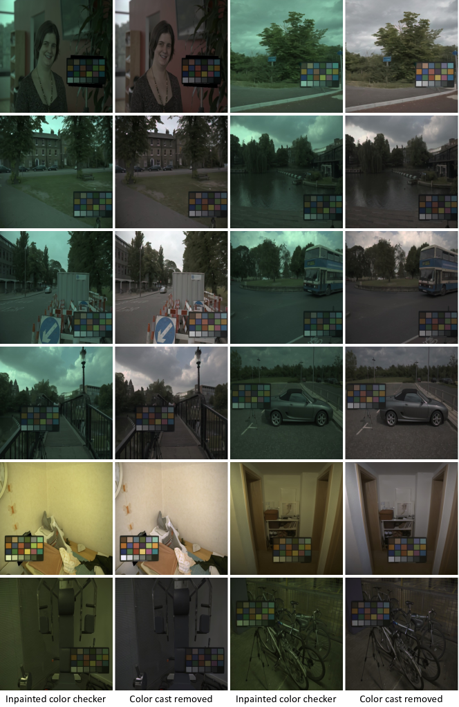
Figure 10: Qualitative results for the Gehler dataset.

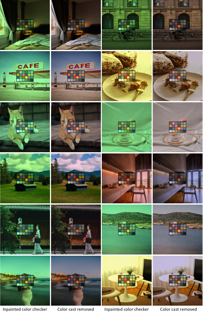
Figure 11: Qualitative results for in-the-wild images with center-placed color checkers.

References

- Afifi and Brown [2019] Mahmoud Afifi and Michael S Brown. Sensor-independent illumination estimation for dnn models. In BMVC, 2019.
- Afifi et al. [2021] Mahmoud Afifi, Jonathan T Barron, Chloe LeGendre, Yun-Ta Tsai, and Francois Bleibel. Cross-camera convolutional color constancy. In Proceedings of the IEEE/CVF International Conference on Computer Vision, 2021.
- Akimoto et al. [2019] Naofumi Akimoto, Seito Kasai, Masaki Hayashi, and Yoshimitsu Aoki. 360-degree image completion by two-stage conditional gans. In 2019 IEEE International Conference on Image Processing (ICIP), pages 4704–4708. IEEE, 2019.
- Avrahami et al. [2022] Omri Avrahami, Dani Lischinski, and Ohad Fried. Blended diffusion for text-driven editing of natural images. In Proceedings of the IEEE/CVF Conference on Computer Vision and Pattern Recognition (CVPR), pages 18208–18218, 2022.
- Avrahami et al. [2023] Omri Avrahami, Ohad Fried, and Dani Lischinski. Blended latent diffusion. ACM Trans. Graph., 42(4), 2023.
- Barnard [2000] Kobus Barnard. Improvements to gamut mapping colour constancy algorithms. In European conference on computer vision, 2000.
- Barnard et al. [2002] Kobus Barnard, Vlad Cardei, and Brian Funt. A comparison of computational color constancy algorithms. i: Methodology and experiments with synthesized data. IEEE transactions on Image Processing, 11(9):972–984, 2002.
- Barron [2015] Jonathan T Barron. Convolutional color constancy. In International Conference on Computer Vision, 2015.
- Barron and Tsai [2017] Jonathan T Barron and Yun-Ta Tsai. Fast fourier color constancy. In Computer Vision and Pattern Recognition, 2017.
- Bianco and Cusano [2019] Simone Bianco and Claudio Cusano. Quasi-unsupervised color constancy. In Proceedings of the IEEE/CVF Conference on Computer Vision and Pattern Recognition, 2019.
- Brainard and Wandell [1986] David H Brainard and Brian A Wandell. Analysis of the retinex theory of color vision. JOSA A, 3(10):1651–1661, 1986.
- Buchsbaum [1980] Gershon Buchsbaum. A spatial processor model for object colour perception. Journal of the Franklin institute, 1980.
- Calian et al. [2018] Dan A Calian, Jean-François Lalonde, Paulo Gotardo, Tomas Simon, Iain Matthews, and Kenny Mitchell. From faces to outdoor light probes. In Computer Graphics Forum, pages 51–61. Wiley Online Library, 2018.
- Chakrabarti [2015] Ayan Chakrabarti. Color constancy by learning to predict chromaticity from luminance. Advances in Neural Information Processing Systems, 28, 2015.
- Chakrabarti et al. [2011] Ayan Chakrabarti, Keigo Hirakawa, and Todd Zickler. Color constancy with spatio-spectral statistics. IEEE Transactions on Pattern Analysis and Machine Intelligence, 2011.
- Cheng et al. [2014a] Dongliang Cheng, Dilip K. Prasad, and Michael S. Brown. Illuminant estimation for color constancy: why spatial-domain methods work and the role of the color distribution. J. Opt. Soc. Am. A, 31(5):1049–1058, 2014a.
- Cheng et al. [2014b] Dongliang Cheng, Dilip K Prasad, and Michael S Brown. Illuminant estimation for color constancy: why spatial-domain methods work and the role of the color distribution. JOSA A, 31(5):1049–1058, 2014b.
- Dastjerdi et al. [2022] Mohammad Reza Karimi Dastjerdi, Yannick Hold-Geoffroy, Jonathan Eisenmann, Siavash Khodadadeh, and Jean-François Lalonde. Guided co-modulated gan for 360° field of view extrapolation. In 2022 International Conference on 3D Vision (3DV), pages 475–485. IEEE, 2022.
- Dastjerdi et al. [2023] Mohammad Reza Karimi Dastjerdi, Jonathan Eisenmann, Yannick Hold-Geoffroy, and Jean-François Lalonde. Everlight: Indoor-outdoor editable hdr lighting estimation. In Proceedings of the IEEE/CVF International Conference on Computer Vision, pages 7420–7429, 2023.
- Daume III and Marcu [2006] Hal Daume III and Daniel Marcu. Domain adaptation for statistical classifiers. Journal of artificial Intelligence research, 2006.
- Debevec [1998] Paul Debevec. Rendering synthetic objects into real scenes: Bridging traditional and image-based graphics with global illumination and high dynamic range photography. In Proceedings of the 25th Annual Conference on Computer Graphics and Interactive Techniques, page 189–198, New York, NY, USA, 1998. Association for Computing Machinery.
- Dhariwal and Nichol [2021] Prafulla Dhariwal and Alexander Nichol. Diffusion models beat gans on image synthesis. Advances in neural information processing systems, 2021.
- Finlayson and Trezzi [2004] Graham D Finlayson and Elisabetta Trezzi. Shades of gray and colour constancy. In Color and Imaging Conference, 2004.
- Funt and Xiong [2004] Brian Funt and Weihua Xiong. Estimating illumination chromaticity via support vector regression. In Color and Imaging Conference, 2004.
- Gal et al. [2022] Rinon Gal, Yuval Alaluf, Yuval Atzmon, Or Patashnik, Amit H Bermano, Gal Chechik, and Daniel Cohen-Or. An image is worth one word: Personalizing text-to-image generation using textual inversion. arXiv preprint arXiv:2208.01618, 2022.
- Gao et al. [2014] Shaobing Gao, Wangwang Han, Kaifu Yang, Chaoyi Li, and Yongjie Li. Efficient color constancy with local surface reflectance statistics. In Computer Vision–ECCV 2014: 13th European Conference, Zurich, Switzerland, September 6-12, 2014, Proceedings, Part II 13, pages 158–173. Springer, 2014.
- Gao et al. [2017] Shao-Bing Gao, Ming Zhang, Chao-Yi Li, and Yong-Jie Li. Improving color constancy by discounting the variation of camera spectral sensitivity. JOSA A, 2017.
- Garcia et al. [2024] Gonzalo Martin Garcia, Karim Abou Zeid, Christian Schmidt, Daan de Geus, Alexander Hermans, and Bastian Leibe. Fine-tuning image-conditional diffusion models is easier than you think. arXiv preprint arXiv:2409.11355, 2024.
- Gardner et al. [2017] Marc-André Gardner, Kalyan Sunkavalli, Ersin Yumer, Xiaohui Shen, Emiliano Gambaretto, Christian Gagné, and Jean-François Lalonde. Learning to predict indoor illumination from a single image. ACM Trans. Graph., 36(6), 2017.
- Garon et al. [2019] Mathieu Garon, Kalyan Sunkavalli, Sunil Hadap, Nathan Carr, and Jean-François Lalonde. Fast spatially-varying indoor lighting estimation. In Proceedings of the IEEE/CVF Conference on Computer Vision and Pattern Recognition, pages 6908–6917, 2019.
- Gehler et al. [2008a] Peter Vincent Gehler, Carsten Rother, Andrew Blake, Tom Minka, and Toby Sharp. Bayesian color constancy revisited. In 2008 IEEE Conference on Computer Vision and Pattern Recognition, pages 1–8, 2008a.
- Gehler et al. [2008b] Peter Vincent Gehler, Carsten Rother, Andrew Blake, Tom Minka, and Toby Sharp. Bayesian color constancy revisited. In 2008 IEEE Conference on Computer Vision and Pattern Recognition, pages 1–8. IEEE, 2008b.
- Han et al. [2023] Ligong Han, Yinxiao Li, Han Zhang, Peyman Milanfar, Dimitris Metaxas, and Feng Yang. Svdiff: Compact parameter space for diffusion fine-tuning. arXiv preprint arXiv:2303.11305, 2023.
- Hold-Geoffroy et al. [2017] Yannick Hold-Geoffroy, Kalyan Sunkavalli, Sunil Hadap, Emiliano Gambaretto, and Jean-François Lalonde. Deep outdoor illumination estimation. In Proceedings of the IEEE conference on computer vision and pattern recognition, pages 7312–7321, 2017.
- Hosek and Wilkie [2012] Lukas Hosek and Alexander Wilkie. An analytic model for full spectral sky-dome radiance. ACM Transactions on Graphics (TOG), 31(4):1–9, 2012.
- Hu et al. [2021] Edward J Hu, Yelong Shen, Phillip Wallis, Zeyuan Allen-Zhu, Yuanzhi Li, Shean Wang, Lu Wang, and Weizhu Chen. Lora: Low-rank adaptation of large language models. arXiv preprint arXiv:2106.09685, 2021.
- Hu et al. [2017] Yuanming Hu, Baoyuan Wang, and Stephen Lin. Fc4: Fully convolutional color constancy with confidence-weighted pooling. In Computer Vision and Pattern Recognition, 2017.
- Joze et al. [2012] Hamid Reza Vaezi Joze, Mark S Drew, Graham D Finlayson, and Perla Aurora Troncoso Rey. The role of bright pixels in illumination estimation. In Color and Imaging Conference, 2012.
- Karsch et al. [2011] Kevin Karsch, Varsha Hedau, David Forsyth, and Derek Hoiem. Rendering synthetic objects into legacy photographs. ACM Transactions on graphics (TOG), 30(6):1–12, 2011.
- Ke et al. [2024] Bingxin Ke, Anton Obukhov, Shengyu Huang, Nando Metzger, Rodrigo Caye Daudt, and Konrad Schindler. Repurposing diffusion-based image generators for monocular depth estimation. In Proceedings of the IEEE/CVF Conference on Computer Vision and Pattern Recognition, pages 9492–9502, 2024.
- Kingma et al. [2021] Diederik Kingma, Tim Salimans, Ben Poole, and Jonathan Ho. Variational diffusion models. Advances in neural information processing systems, 2021.
- LeGendre et al. [2019] Chloe LeGendre, Wan-Chun Ma, Graham Fyffe, John Flynn, Laurent Charbonnel, Jay Busch, and Paul Debevec. Deeplight: Learning illumination for unconstrained mobile mixed reality. In Proceedings of the IEEE/CVF Conference on Computer Vision and Pattern Recognition, 2019.
- Liba et al. [2019] Orly Liba, Kiran Murthy, Yun-Ta Tsai, Tim Brooks, Tianfan Xue, Nikhil Karnad, Qiurui He, Jonathan T Barron, Dillon Sharlet, Ryan Geiss, et al. Handheld mobile photography in very low light. ACM Trans. Graph., 2019.
- Lin et al. [2024] Shanchuan Lin, Bingchen Liu, Jiashi Li, and Xiao Yang. Common diffusion noise schedules and sample steps are flawed. In Proceedings of the IEEE/CVF winter conference on applications of computer vision, 2024.
- Lo et al. [2021] Yi-Chen Lo, Chia-Che Chang, Hsuan-Chao Chiu, Yu-Hao Huang, Chia-Ping Chen, Yu-Lin Chang, and Kevin Jou. Clcc: Contrastive learning for color constancy. In Proceedings of the IEEE/CVF Conference on Computer Vision and Pattern Recognition, 2021.
- Lombardi and Nishino [2015] Stephen Lombardi and Ko Nishino. Reflectance and illumination recovery in the wild. IEEE transactions on pattern analysis and machine intelligence, 38(1):129–141, 2015.
- Meng et al. [2022] Chenlin Meng, Yutong He, Yang Song, Jiaming Song, Jiajun Wu, Jun-Yan Zhu, and Stefano Ermon. Sdedit: Guided image synthesis and editing with stochastic differential equations, 2022.
- Nishino and Nayar [2004] Ko Nishino and Shree K Nayar. Eyes for relighting. ACM Transactions on Graphics (TOG), 23(3):704–711, 2004.
- Phongthawee et al. [2024] Pakkapon Phongthawee, Worameth Chinchuthakun, Nontaphat Sinsunthithet, Varun Jampani, Amit Raj, Pramook Khungurn, and Supasorn Suwajanakorn. Diffusionlight: Light probes for free by painting a chrome ball. In Proceedings of the IEEE/CVF Conference on Computer Vision and Pattern Recognition, pages 98–108, 2024.
- Qian et al. [2019] Yanlin Qian, Joni-Kristian Kamarainen, Jarno Nikkanen, and Jiri Matas. On finding gray pixels. In Computer Vision and Pattern Recognition, 2019.
- Qiu et al. [2023] Zeju Qiu, Weiyang Liu, Haiwen Feng, Yuxuan Xue, Yao Feng, Zhen Liu, Dan Zhang, Adrian Weller, and Bernhard Schölkopf. Controlling text-to-image diffusion by orthogonal finetuning. arXiv preprint arXiv:2306.07280, 2023.
- Rombach et al. [2021] Robin Rombach, Andreas Blattmann, Dominik Lorenz, Patrick Esser, and Björn Ommer. High-resolution image synthesis with latent diffusion models, 2021.
- Ronneberger et al. [2015] Olaf Ronneberger, Philipp Fischer, and Thomas Brox. U-net: Convolutional networks for biomedical image segmentation. In Medical image computing and computer-assisted intervention–MICCAI 2015: 18th international conference, Munich, Germany, October 5-9, 2015, proceedings, part III 18, 2015.
- Ruiz et al. [2022] Nataniel Ruiz, Yuanzhen Li, Varun Jampani, Yael Pritch, Michael Rubinstein, and Kfir Aberman. Dreambooth: Fine tuning text-to-image diffusion models for subject-driven generation. arXiv preprint arXiv:2208.12242, 2022.
- Saenko et al. [2010] Kate Saenko, Brian Kulis, Mario Fritz, and Trevor Darrell. Adapting visual category models to new domains. In Computer Vision–ECCV 2010: 11th European Conference on Computer Vision, Heraklion, Crete, Greece, September 5-11, 2010, Proceedings, Part IV 11, 2010.
- Shi [2000] Lilong Shi. Re-processed version of the gehler color constancy dataset of 568 images. http://www. cs. sfu. ca/˜ color/data/, 2000.
- Sohl-Dickstein et al. [2015] Jascha Sohl-Dickstein, Eric Weiss, Niru Maheswaranathan, and Surya Ganguli. Deep unsupervised learning using nonequilibrium thermodynamics. In International conference on machine learning, 2015.
- van de Weijer et al. [2007] Joost van de Weijer, Theo Gevers, and Arjan Gijsenij. Edge-based color constancy. IEEE Trans. Image Process., pages 2207–2214, 2007.
- Van De Weijer et al. [2007] Joost Van De Weijer, Theo Gevers, and Arjan Gijsenij. Edge-based color constancy. IEEE Transactions on image processing, 16(9):2207–2214, 2007.
- Voynov et al. [2023] Andrey Voynov, Qinghao Chu, Daniel Cohen-Or, and Kfir Aberman. P+: Extended textual conditioning in text-to-image generation. 2023.
- Wang et al. [2022] Guangcong Wang, Yinuo Yang, Chen Change Loy, and Ziwei Liu. Stylelight: Hdr panorama generation for lighting estimation and editing. In European Conference on Computer Vision, pages 477–492. Springer, 2022.
- Weber et al. [2018] Henrique Weber, Donald Prévost, and Jean-François Lalonde. Learning to estimate indoor lighting from 3d objects. In 2018 International Conference on 3D Vision (3DV), pages 199–207. IEEE, 2018.
- Xu et al. [2020] Bolei Xu, Jingxin Liu, Xianxu Hou, Bozhi Liu, and Guoping Qiu. End-to-end illuminant estimation based on deep metric learning. In Proceedings of the IEEE/CVF Conference on Computer Vision and Pattern Recognition, 2020.
- Yang et al. [2023] Binxin Yang, Shuyang Gu, Bo Zhang, Ting Zhang, Xuejin Chen, Xiaoyan Sun, Dong Chen, and Fang Wen. Paint by example: Exemplar-based image editing with diffusion models. In Proceedings of the IEEE/CVF Conference on Computer Vision and Pattern Recognition, pages 18381–18391, 2023.
- Yang et al. [2015] Kai-Fu Yang, Shao-Bing Gao, and Yong-Jie Li. Efficient illuminant estimation for color constancy using grey pixels. In Proceedings of the IEEE conference on computer vision and pattern recognition, pages 2254–2263, 2015.
- Ye et al. [2023] Hu Ye, Jun Zhang, Sibo Liu, Xiao Han, and Wei Yang. Ip-adapter: Text compatible image prompt adapter for text-to-image diffusion models. 2023.
- Yi et al. [2018] Renjiao Yi, Chenyang Zhu, Ping Tan, and Stephen Lin. Faces as lighting probes via unsupervised deep highlight extraction. In Proceedings of the European Conference on computer vision (ECCV), pages 317–333, 2018.
- Yu et al. [2020] Huanglin Yu, Ke Chen, Kaiqi Wang, Yanlin Qian, Zhaoxiang Zhang, and Kui Jia. Cascading convolutional color constancy. In Proceedings of the AAAI Conference on Artificial Intelligence, pages 12725–12732, 2020.
- Zhang et al. [2023] Lvmin Zhang, Anyi Rao, and Maneesh Agrawala. Adding conditional control to text-to-image diffusion models, 2023.