Dynamical phases of short-term memory mechanisms in RNNs
Abstract
Short-term memory is essential for cognitive processing, yet our understanding of its neural mechanisms remains unclear. A key focus in neuroscience has been the study of sequential activity patterns, where neurons fire one after another within large networks, to explain how information is maintained. While recurrent connections were shown to drive sequential dynamics, a mechanistic understanding of this process still remains unknown. In this work, we first introduce two unique mechanisms that can subserve short-term memory: slow-point manifolds generating direct sequences or limit cycles providing temporally localized approximations. Then, through analytical models, we identify fundamental properties that govern the selection of these mechanisms, i.e., we derive theoretical scaling laws for critical learning rates as a function of the delay period length, beyond which no learning is possible. We empirically verify these observations by training and evaluating more than 35,000 recurrent neural networks (RNNs) that we will publicly release upon publication. Overall, our work provides new insights into short-term memory mechanisms and proposes experimentally testable predictions for systems neuroscience.
1 Introduction
Short-term memory is the process through which both biological and artificial systems are able to store information for a short period of time. This process is essential for adaptive behavior, which is disrupted in several neurological and psychiatric conditions such as Alzheimer’s disease [1], schizophrenia [2] and post-traumatic stress disorder [3] among others. Yet, while short-term memory is a central function in mammalian cognition, the mechanisms that subserve it remain an open question in systems neuroscience [4].
In both humans and animals, short-term memory has been shown to be supported through a distributed dynamic network across cortical regions such as prefrontal, parietal and sensory regions [5, 6, 7, 8, 9, 10, 11]. At the neuronal level, persistent neuronal activity has been linked to the memory maintenance period [8, 12, 6, 13] (Fig. 1). Some other evidence showed that short-term memory can also be supported in the form of sequential neuronal activations [9, 14, 15, 16] (Fig. 1). However, growing evidence suggests distributed and dynamic firing patterns across the neuronal population [10, 17, 11], where memory stability and robustness is achieved through attractor dynamics [18, 19]. It is unclear what are the different factors influencing how memory is maintained in the neuronal activities, what is the underlying mechanism, and how it changes over extended delay periods.
Here we set out to answer these questions through a computational theory perspective, which in turn provide experimental testable predictions. To achieve that, we trained over 35,000 RNNs to perform delayed cue discrimination tasks, while studied simple toy models and low-rank RNN models as they performed a simplified delayed activation task. In our tasks, neural activation sequences emerged as the precursor of the solutions. These sequences were generated through two distinct mechanisms: slow-point manifolds and limit cycles. Surprisingly, limit cycles emerged naturally to approximate neuronal sequences, even though the task had no periodicity component, offering a novel mechanism on how these sequences may be generated in the brain. An analytical study revealed that the selection of the mechanism (i.e. slow-point manifold or limit cycles) responsible for the sequences depended on both the task structure and the learning rate of the RNNs. Overall, our results provide new insights and testable experimental predictions for systems neuroscience. We summarize our unique contributions in this paper below:
- •
-
•
We show how changing one of the simplest tasks in a trivial manner, e.g., by adding a post-reaction period, can qualitatively change the learned short-term memory mechanisms. This finding is particularly relevant as a cautionary tale for the systems neuroscience community modeling animal behaviors by drawing comparisons to RNNs [20] (Fig. 4).
-
•
Utilizing analytical models, we demonstrate theoretical scaling laws and synthesize a phase diagram of mechanisms for solving the task, which is a function of the task properties and optimization parameters (Fig. 5).
-
•
Through a large-scale study of over 35,000 RNNs (which will be made publicly available), we extract scaling laws in RNNs trained to perform delayed cue-discrimination tasks. We show that RNNs have little to no trouble learning a modified task with no delayed output, providing further evidence that training neural networks to delay their outputs is a fundamentally difficult problem (Figs. 6, 7, S1, and S2).

2 Background
Systems neuroscience often utilizes animal models, e.g., mice, rats, birds, flies, to study cognitive functions including short-term memory [4]. Similarly, it is often possible to design artificial models such as RNNs, which can be trained on observed neural activities or tasks that are traditionally performed by animals in laboratories [20, 23, 24, 25, 26]. Then, once RNNs are trained, their computation can be reverse-engineered to draw potential inferences to the nature of the neural computation performed by biological networks that can later be tested with experimental procedures [27, 28]. Consequently, RNNs have recently become a key component of computational neuroscience studies [26, 29, 28, 23].
Due to their biological relevance and easy interpretation of their parameters as functional connections between neurons [30, 31], in this work, we study RNNs with the following set of equations:
| (1) |
where refers to the firing rates, pre-defined inputs, weight parameters and corresponding bias terms, and some noise that is, in practice, sampled iid from a Gaussian distribution. The output is taken as a projection of the neural activities as , where is either identity or sigmoid function in this work (see below). For notational simplicity, we assume until our empirical results in Section 3.4.
Recent work has shown that when are constrained to be low-rank, the computation performed by RNNs can be written in terms of a latent dynamical system [26, 29, 32]:
| (2) |
where the latent variables are defined as [32]. Intuitively, by constraining the rank of the weight matrix, , one can project the computation performed by neurons down to -dimensional latent dynamical systems. When we study low-rank RNNs, we define the network output as a nonlinear projection from the latent variables with a sigmoid function . In this work, we use this paradigm (i.e., training low-rank RNNs) to illustrate the distinct mechanisms that can emerge during training to support sequence generation. Then, our large-scale experiments generalize our findings to full-rank RNNs with no explicit restrictions.
3 Results
Using a slightly modified version111which is nonetheless computationally equivalent after a simple transformation of variables [33]. of the architecture in Eq. (1), recent work has identified generation of neural sequences as a potential key component of short-term memory [15]. This sequence then can be used to store the short-term memory content, while allowing to explicitly keep track of the time, as opposed to earlier theories of short-term memory maintenance that relied on persistent activities of some neural populations [21, 22] (Fig. 1). Previous work has provided insights into how these sequences are generated by examining neuronal-level mechanisms [15, 34, 35], often focusing on the learned connectivity structures [15, 35]. However, the causal mechanisms underlying neural computation, which could be investigated through latent dynamics, remain largely unexplored.
3.1 RNNs can generate neural sequences using distinct mechanisms
As a first step, we set out to design a simple short-term memory task, where any extra component is stripped away, that can be solved using neural sequences but not persistent firings of the same groups of neurons (Fig. 1). Inspired by the delayed cue discrimination tasks regularly studied in systems neuroscience [36], we started by considering a delayed activation task [37]. In this task, the network is initialized to a particular state, which is randomly selected in the state space (Methods), and has to withhold its response () for a time window. Afterwards, the network is forced to output a response () for time window.
Notably, such a task requires at least two distinct neural activity patterns in two periods and therefore cannot be solved by persistent activity of a subset of neurons. Instead, when we trained rank-2 RNNs to solve the delayed activation task, we observed the emergence of neural sequences (Fig. 2). Interestingly, when we studied the flow maps of the learned dynamical systems, we observed that both limit cycles and a mechanism utilizing slow-points (from now on referred to as “SP manifolds” for generality) could generate the desired sequence in the trial window. Despite having equivalent results within the trial window, the two mechanisms had qualitatively different behaviors after the trial concluded (Fig. 2). Limit cycles had led to recurrent generations of the same sequences, whereas the SP manifolds converged to a persistent activity style representation. Here, we observed that, for a given delay interval , networks tended to form limit cycles when trained with large learning rates, but could form SP manifolds in lower learning rates (Fig. 2). We will make this observation rigorous in our large-scale studies below, but for now, we asked the question: Do RNNs commit to learning one mechanism from the start, or are they capable of changing their inner mechanisms during the training?
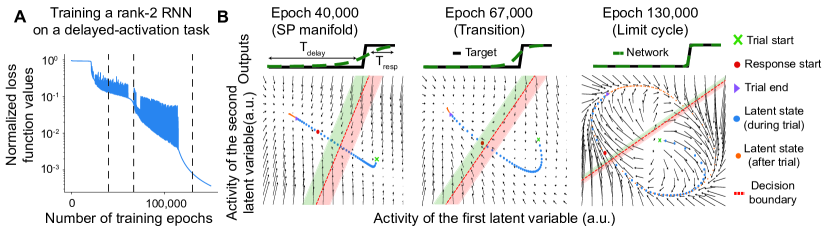
To answer this question, we studied the latent dynamical systems of a rank-2 RNN as it was solving the delayed activation task (Fig. 3). Interestingly, the loss function showed characteristic periods of learning, corresponding to changes in mechanisms (Fig. 3A). Specifically, after the first jump in the loss function, a SP manifold was formed in the latent dynamical system (Fig. 3B; left). Here, a line of slow-points allowed the network output to stall until . Then, the SP manifold had acquired a curved structure (Fig. 3B; middle), reminiscent of a transitory solution. Finally, after the oscillations in the loss function values ceased, a limit cycle had emerged in the latent dynamical system (Fig. 3B; right). Hence, we confirmed that RNNs could change their inner mechanisms during learning, i.e., what started as a SP manifold solution later evolved into a limit cycle.
In reality, since functional connections in the brain can rapidly reorganize within the start and end of a trial [36], the two mechanisms can become practically inseparable in biological networks. In other words, there is an equivalence class of mechanisms that can generate neural sequences that have the same local behavior within the task window, but can show distinct properties outside; and the two mechanisms we identified belong to this class. For the rest of this work, we aim to understand whether these mechanisms emerge randomly, or whether there is some structure to which mechanism is learned by the network based on task and optimization parameters.
![[Uncaptioned image]](/html/2502.17433/assets/x2.png)
3.2 Influence of task design on the learned latent mechanism
Behavioral experiments in systems neuroscience often contain arbitrary design choices that are deeply embedded in the experimental paradigm, yet their implications are rarely scrutinized. Consider the delayed cue discrimination task, which is similar to the delayed activation task, but with two input and output channels where the delay period begins after a brief cue presentation window (, discussed below in Fig. 6). While animals typically indicate their response by licking either a right or left spout, seemingly minor procedural decisions – such as whether to provide immediate feedback or require a short post-response waiting period – can fundamentally alter the mechanisms networks learn to solve the task.
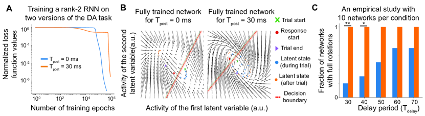
Our investigations reveal that implementing a post-reaction period qualitatively changes the dynamical mechanisms emerging in trained networks. In our delayed activation task, we already assume that a previous cue has put the network in a stereotypical state, hence the initialization to a particular state in the task. Then, we can consider our toy tasks as simplified versions of cue discrimination tasks, where we focus on the retention of a particular cue. With this in mind, in networks trained without a post-reaction period (), the dynamics typically converge to stable point attractors, creating a straightforward mapping between stimuli and responses. However, when we introduce even a brief post-reaction period (), the networks predominantly learn limit cycle solutions, despite achieving similar task performance (Fig. 4A). The phase portraits in Fig. 4B clearly illustrate this distinction, showing fixed point convergence in networks without a post-period versus circular trajectories indicating limit cycles in networks with a post-period.
This finding becomes particularly intriguing in the context of the current emphasis on dynamical systems approaches in neuroscience, where considerable attention has been given to identifying and manipulating ([39, 40]) attractors and manifolds underlying neural activity. The stark difference in dynamical solutions – stable points versus limit cycles – emerging from such a minor task modification raises important questions about the interpretation of dynamical structures observed in neural recordings. Can we definitively claim that one dynamical solution is more fundamental than another simply because we observed it in animals performing a particular variant of a task?
To systematically investigate this phenomenon, we conducted a broader empirical study examining how delay period duration interacts with the presence of a post-reaction window (Fig. 4C). Our results demonstrate that increasing the delay period generally promotes the emergence of limit cycle solutions, but this tendency is dramatically amplified by the addition of a post-reaction window. Statistical analysis using Fisher’s exact test with Bonferroni corrections confirms the significance of these effects across different delay periods. These findings serve as a crucial reminder about the profound influence of experimental design choices on the neural mechanisms we observe and interpret. They suggest that we must exercise greater caution when drawing conclusions about the fundamental nature of neural computations based on specific task implementations, as the observed dynamical structures may be more contingent on subtle task parameters than previously appreciated.
3.3 A theoretical scaling analysis of mechanistic phases via toy dynamical system models
So far, we used simple examples to demonstrate how RNNs can use different latent mechanisms to generate sequences, that the choice between mechanisms is not random, and that RNNs can change their inner mechanisms during the course of their training. Now, we turn to a set of toy models and provide theoretical insights into why these phenomena occur.
Previous work has considered a simple toy dynamical system model, the normal form for the saddle-node bifurcation [41], given as for a trainable parameter [37]. Earlier work studied the complex learning dynamics in a simple system that can generate slow-points. In this section, we set out to extend this analysis to a second toy model, a limit cycle attractor. But first, in Appendix S1.1, we reproduce the findings of the earlier work for a more general version of the delayed-activation task with . This analysis reveals a maximum learning rate, also reported in [37], beyond which the learning dynamics destabilize and even an approximation of the desirable solution cannot be reached. Our analysis reveals that the learning rate scales following a power law such that , where . Such a steep decrease with the desirable learning rate can explain our anecdotal observations in Fig. 2 that slow-points become rarer for large or high learning rate values.
Now, we introduce a new toy model that models the limit cycles that follows a two-dimensional dynamical system with periodic orbits. For simplicity, we fix the radius to an attractive fixed-point, and allow a periodic oscillation in the frequency such that the equations of the motion for the toy model become (See Appendix S1.2 for derivations):
| (3) |
where is a learnable parameter and the network output is defined as , where is defined as the Heaviside function. By inspection, the rotations have a half-period of , and the model outputs zero for the first while outputting one for the second half. An example flow map for this model is shown in Fig. 5A. Changing the parameter simply updates the speed of the limit cycle, though as we show below, this is not a trivial task.
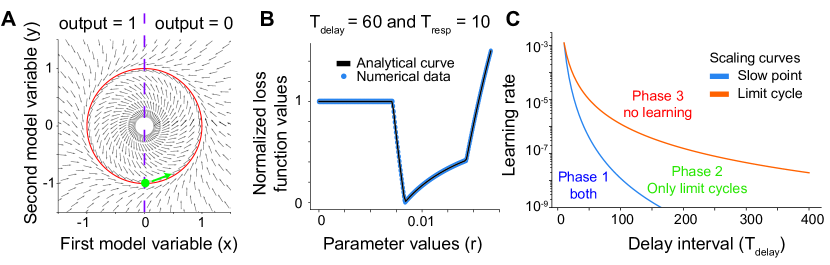
In Appendix S1.2, we compute an analytical loss function for the limit cycle model in the limits and . We illustrate the latter case in Fig. 5B, note the exact correspondence between the analytical curve and the numerical simulations. For both cases, the loss function has a global optimum at . However, it has a kink around the global minimum and quickly flattens to a constant value for . Hence, if the learning rate is larger than some critical value, the oscillations around the global minimum can throw the parameter to a value , terminating the training process due to the zero gradient despite the fact that the model cannot solve the task. Our analysis reveals that this learning rate scales following where . Notably, the limit cycle solution has a better scaling than the slow-point one, providing a theoretical explanation for our observation in Fig. 3. Specifically, since the RNN in Fig. 3 was trained using a learning rate right at the transition (Compare to Fig. 2), it is not surprising that a slow point mechanism eventually evolves into a limit cycle. Moreover, this theoretical prediction is also consistent with the experiments in Fig. 4C, where increasing the delay period for a fixed learning rate resulted in more RNNs finding limit cycle based solutions. Similarly, by simply shifting the decision boundary from to for some , this model can also incorporate a post-reaction period of zero outputs, for instance by setting the total period equal to .
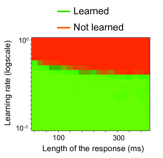
At least as interesting is the fact that the different scaling of these solutions defines a phase space of mechanisms that can be learned by RNNs. This phase space, illustrated in Fig. 5C, depends on the delay time (a task parameter) and the learning rate (an optimization parameter). Below, we show empirically that similar phase diagrams emerge in full-rank RNNs trained on delayed cue discrimination tasks. It is worth noting that increasing the dimensionality of the dynamical system can allow more efficient solutions to the system, but the toy models we discuss can be thought as approximate bounds on what can be achieved.
3.4 A large-scale analysis with RNNs reveals an empirical scaling law and mechanistic phases
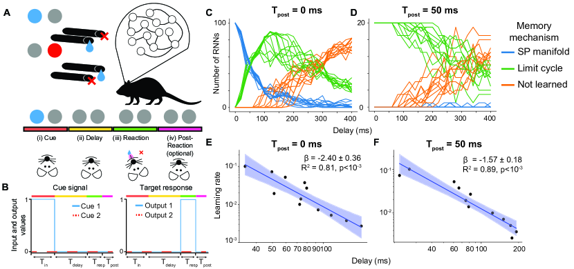
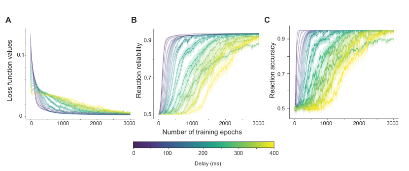
Next, we tested our theoretical predictions by training over 35,000 RNNs on delayed cue-discrimination tasks (Figs. 6 and S1). Briefly, delayed cue-discrimination task consists of four distinct periods: cue, delay, reaction, and an optional post-reaction period (i-iv). Upon observation of a cue, the networks have to wait for a brief period and output a response in the corresponding output channel. If there is a post-reaction period, then the networks should learn to output zeros after the response window concludes.
First, we examined whether different mechanisms would consistently emerge in different values of the delay windows, as predicted by our theoretical analysis earlier. In Fig. 6 (C-D), we observed that increasing the length of the delay period preferentially led to the emergence of limit cycles, consistent with our findings in Figs. 2 and 3. Yet, RNNs still developed slow-point manifolds for shorter delays, which was nonetheless absent for RNNs performing a modified version of the task with a post-reaction window (Fig. 6 (C-D)). Notably, when we trained on a version of the task that no longer required a memory maintenance component (Fig. S2), the dependence on the full length of the trial was minimal and the relationship observed in Fig. 6C-D was practically ablated. Therefore, overall, these results suggested that task requirements shape the viability of different memory strategies.
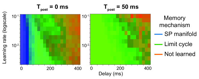
Next, we quantified the relationship between delay duration and learning performance through scaling law analysis (Fig 6E-F). The critical exponent differed significantly between the original task () and the modified version with post-reaction period (). Interestingly, however, the critical exponent extracted from the former was within the expected range of values from our theoretical studies using the delayed activation task. Finally, to comprehensively map these mechanistic transitions, we plotted a phase diagram (Fig 7) that captures both the emergence of different memory mechanisms and their associated scaling laws.
4 Discussion
Learning to respond based on delayed information is a fundamental challenge in both neuroscience and machine learning [42, 43]. In machine learning, early studies in the 1990s identified this difficulty as the problem of learning long-term dependencies, particularly in recurrent neural networks (RNNs) trained on tasks requiring information retention across time [43]. Despite significant progress in neural network architectures, this issue remains central to designing systems capable of effective temporal reasoning.
To address long-term dependencies, researchers developed specialized architectures such as Long Short-Term Memory (LSTM) networks, Gated Recurrent Units (GRUs), and, more recently, Transformers [44, 45, 46]. These models introduced mechanisms that improved memory retention by adjusting internal timescales. However, unlike biological neurons, which operate under fixed timescales—such as the “membrane time constant,” which governs the decay of neuronal firing [47, 48, 49, 50, 51]—these architectures learn their own timescales dynamically. This fundamental difference raises the question: why do biologically inspired networks struggle to learn long-term dependencies, and what constraints govern their performance?
A key insight into this question comes from examining the relationship between learning rate and delay length. In simple delayed-response tasks, we show that the maximum learning rate, beyond which training fails, follows a power-law scaling with delay length. This implies that as the delay increases, learning requires increasingly small updates, ultimately rendering training impractically slow for long delays. This limitation may have played a role in capturing long-term dependencies, which was the focus of the early RNN studies [43].
The development of gated architectures such as LSTMs and GRUs helped alleviate this issue by introducing adaptive timescales, allowing networks to modulate how past information is retained [44]. In principle, flexible timescales can overcome the power-law limitation of fixed dynamical systems. However, this comes at a cost. Extending timescales indefinitely would slow down computation, making rapid decision-making difficult. Moreover, increasing the parameter space to accommodate longer memory spans complicates optimization, potentially destabilizing learning [37]. Unlike biological networks, which are constrained by predefined timescales such as action potentials, artificial networks rely on optimizing these scales through training—a difference that influences their ability to generalize across temporal tasks.
Understanding these fundamental constraints provides a new perspective on why learning long-term dependencies is difficult across different architectures. By framing the problem through the lens of dynamical systems theory, we characterized a crucial trade-off as part of this problem. The identification of this trade-off may allow future work to explore potential solutions that balance biological plausibility, computational efficiency, and learning performance.
Our work also has implications for experimental neuroscience. Specifically, limit cycles have been studied in terms of phase matching (i.e., periodic computation) [52]. But, here we have shown that more generally, they can also be used to approximate sequential neuronal activations. However, in a dynamic brain, where synaptic plasticity changes functional connectivity rapidly [36], how can we figure out whether slow points or limit cycles subserve observed neural dynamics? More broadly, how can we tell apart solutions that locally form a class of equivalence, but are globally distinct. To the best of our knowledge, this unique concept has not been addressed or raised as part of the experimental design in systems neuroscience research. Yet, addressing these questions would require a new style of experiments to be designed. To start with, in this work, we illustrated how different manipulations in the task structure can shed light into dissociating these mechanisms.
Finally, beyond neuroscience, this phenomenon of staged learning dynamics, algorithmic phase transitions, is widely observed in artificial networks including transformers trained on mod-arithmetic tasks [53, 54], language modeling [55, 56], and in-context learning [57]. In these studies of learning dynamics on sequential tasks, our study of RNNs offers a unique perspective on interpretability by connecting the computational mechanisms of circuits to foundational mechanisms in dynamical systems. Furthermore, these recent works [58] aim to identify progress measures of learning, akin to order parameters in physics, to see if phase transitions occur. Here, we see that literal phases emerge with distinct computational mechanisms. Future works could explore ways to functionally map those dynamical mechanisms of computation to mechanisms implementable by feedforward architectures like Transformers.
5 Conclusion
In this work, we explored the mechanisms of how recurrent neural networks developed and utilized different mechanisms for maintaining short-term memory. Through extensive theoretical analysis and empirical validation with over 35,000 trained RNNs, we identified two distinct memory maintenance strategies that subserved the emergence of neural sequences: slow-point manifolds and limit cycles. We demonstrated that the emergence of these mechanisms followed scaling laws relating learning rates to delay periods, and showed how subtle changes in task structure (like adding a post-reaction period) could fundamentally alter which mechanism predominated. Our findings have important implications for both machine learning and neuroscience - they help explain why learning long-term dependencies is inherently difficult in neural networks with fixed timescales, and they suggest new experimental approaches for investigating memory mechanisms in biological neural circuits. Most importantly, our work revealed that neural circuits may use multiple, mathematically equivalent mechanisms to solve the same memory task, highlighting the need to carefully consider task design when interpreting neural recordings.
Acknowledgements
We would like to thank members of the Geometric Intelligence Lab for their helpful feedback on an earlier version of the project and Dr. Boris Shraiman for fruitful discussions on the final manuscript. EC and BK’s internships were supported in part by a grant from the Feldman-McClelland Open-a-Door fund of the Pittsburgh Foundation. BK thanks the Impact Scholarship and Research Scholarship for Critical Thinkers programs from the Bridge to Turkiye Funds for supporting his visit to Stanford University. FD expresses gratitude for the valuable mentorship he received at PHI Lab during his internship at NTT Research. MJS gratefully acknowledges funding from the Simons Collaboration on the Global Brain and the Vannevar Bush Faculty Fellowship Program of the U.S. Department of Defense. NM acknowledges funding from the National Science Foundation, award 2313150. FD acknowledges funding from Stanford University’s Mind, Brain, Computation and Technology program, which is supported by the Stanford Wu Tsai Neuroscience Institute. This research was supported in part by grant NSF PHY-2309135 and the Gordon and Betty Moore Foundation Grant No. 2919.02 to the Kavli Institute for Theoretical Physics (KITP). Some of the computing for this project was performed on the Sherlock cluster. We would like to thank Stanford University and the Stanford Research Computing Center for providing computational resources and support that contributed to these research results.
References
- [1] Mark W Bondi, Emily C Edmonds, and David P Salmon. Alzheimer’s disease: past, present, and future. Journal of the International Neuropsychological Society, 23(9-10):818–831, 2017.
- [2] Junghee Lee and Sohee Park. Working memory impairments in schizophrenia: a meta-analysis. Journal of abnormal psychology, 114(4):599, 2005.
- [3] J Cobb Scott, Georg E Matt, Kristen M Wrocklage, Cassandra Crnich, Jessica Jordan, Steven M Southwick, John H Krystal, and Brian C Schweinsburg. A quantitative meta-analysis of neurocognitive functioning in posttraumatic stress disorder. Psychological bulletin, 141(1):105, 2015.
- [4] John T Serences. Neural mechanisms of information storage in visual short-term memory. Vision research, 128:53–67, 2016.
- [5] J Jay Todd and René Marois. Capacity limit of visual short-term memory in human posterior parietal cortex. Nature, 428(6984):751–754, 2004.
- [6] Clayton E Curtis and Mark D’Esposito. Persistent activity in the prefrontal cortex during working memory. Trends in cognitive sciences, 7(9):415–423, 2003.
- [7] Stephenie A Harrison and Frank Tong. Decoding reveals the contents of visual working memory in early visual areas. Nature, 458(7238):632–635, 2009.
- [8] James W Gnadt and Richard A Andersen. Memory related motor planning activity in posterior parietal cortex of macaque. Experimental brain research, 70:216–220, 1988.
- [9] EH Baeg, YB Kim, K Huh, I Mook-Jung, HT Kim, and MW Jung. Dynamics of population code for working memory in the prefrontal cortex. Neuron, 40(1):177–188, 2003.
- [10] Sean E Cavanagh, John P Towers, Joni D Wallis, Laurence T Hunt, and Steven W Kennerley. Reconciling persistent and dynamic hypotheses of working memory coding in prefrontal cortex. Nature communications, 9(1):3498, 2018.
- [11] Ethan M Meyers, David J Freedman, Gabriel Kreiman, Earl K Miller, and Tomaso Poggio. Dynamic population coding of category information in inferior temporal and prefrontal cortex. Journal of neurophysiology, 100(3):1407–1419, 2008.
- [12] Shabtai Barash, R Martyn Bracewell, Leonardo Fogassi, James W Gnadt, and Richard A Andersen. Saccade-related activity in the lateral intraparietal area. i. temporal properties; comparison with area 7a. Journal of neurophysiology, 66(3):1095–1108, 1991.
- [13] Alan D. Baddeley and Graham Hitch. Working memory. volume 8 of Psychology of Learning and Motivation, pages 47–89. Academic Press, 1974.
- [14] Christopher D Harvey, Philip Coen, and David W Tank. Choice-specific sequences in parietal cortex during a virtual-navigation decision task. Nature, 484(7392):62–68, 2012.
- [15] Kanaka Rajan, Christopher D Harvey, and David W Tank. Recurrent network models of sequence generation and memory. Neuron, 90(1):128–142, 2016.
- [16] Xiao-Jing Wang. 50 years of mnemonic persistent activity: quo vadis? Trends in Neurosciences, 44(11):888–902, 2021.
- [17] Eelke Spaak, Kei Watanabe, Shintaro Funahashi, and Mark G Stokes. Stable and dynamic coding for working memory in primate prefrontal cortex. Journal of neuroscience, 37(27):6503–6516, 2017.
- [18] Jake P Stroud, John Duncan, and Máté Lengyel. The computational foundations of dynamic coding in working memory. Trends in Cognitive Sciences, 2024.
- [19] Connor Brennan and Alex Proekt. Attractor dynamics with activity-dependent plasticity capture human working memory across time scales. Communications psychology, 1(1):28, 2023.
- [20] Valerio Mante, David Sussillo, Krishna V Shenoy, and William T Newsome. Context-dependent computation by recurrent dynamics in prefrontal cortex. nature, 503(7474):78–84, 2013.
- [21] Joaquin M Fuster and Garrett E Alexander. Neuron activity related to short-term memory. Science, 173(3997):652–654, 1971.
- [22] Richard C Atkinson and Richard M Shiffrin. Human memory: A proposed system and its control processes. Psychology of Learning and Motivation, 1968.
- [23] David Sussillo and Omri Barak. Opening the black box: low-dimensional dynamics in high-dimensional recurrent neural networks. Neural computation, 25(3):626–649, 2013.
- [24] Guangyu Robert Yang, Madhura R Joglekar, H Francis Song, William T Newsome, and Xiao-Jing Wang. Task representations in neural networks trained to perform many cognitive tasks. Nature neuroscience, 22(2):297–306, 2019.
- [25] Nicolas Y Masse, Guangyu R Yang, H Francis Song, Xiao-Jing Wang, and David J Freedman. Circuit mechanisms for the maintenance and manipulation of information in working memory. Nature neuroscience, 22(7):1159–1167, 2019.
- [26] Alexis Dubreuil, Adrian Valente, Manuel Beiran, Francesca Mastrogiuseppe, and Srdjan Ostojic. The role of population structure in computations through neural dynamics. Nature Neuroscience, pages 1–12, 2022.
- [27] Edgar Y Walker, Fabian H Sinz, Erick Cobos, Taliah Muhammad, Emmanouil Froudarakis, Paul G Fahey, Alexander S Ecker, Jacob Reimer, Xaq Pitkow, and Andreas S Tolias. Inception loops discover what excites neurons most using deep predictive models. Nature neuroscience, 22(12):2060–2065, 2019.
- [28] Arseny Finkelstein, Lorenzo Fontolan, Michael N Economo, Nuo Li, Sandro Romani, and Karel Svoboda. Attractor dynamics gate cortical information flow during decision-making. Nature Neuroscience, 24(6):843–850, 2021.
- [29] Adrian Valente, Jonathan W Pillow, and Srdjan Ostojic. Extracting computational mechanisms from neural data using low-rank rnns. Advances in Neural Information Processing Systems, 35:24072–24086, 2022.
- [30] Matthew G Perich and Kanaka Rajan. Rethinking brain-wide interactions through multi-region ‘network of networks’ models. Current opinion in neurobiology, 65:146–151, 2020.
- [31] Matthew G Perich, Charlotte Arlt, Sofia Soares, Megan E Young, Clayton P Mosher, Juri Minxha, Eugene Carter, Ueli Rutishauser, Peter H Rudebeck, Christopher D Harvey, et al. Inferring brain-wide interactions using data-constrained recurrent neural network models. bioRxiv, pages 2020–12, 2021.
- [32] Fatih Dinc, Marta Blanco-Pozo, David Klindt, Francisco Acosta, Yiqi Jiang, Sadegh Ebrahimi, Adam Shai, Hidenori Tanaka, Peng Yuan, Mark J Schnitzer, et al. Latent computing by biological neural networks: A dynamical systems framework. arXiv preprint arXiv:2502.14337, 2025.
- [33] Fatih Dinc, Adam Shai, Mark Schnitzer, and Hidenori Tanaka. CORNN: Convex optimization of recurrent neural networks for rapid inference of neural dynamics. In Thirty-seventh Conference on Neural Information Processing Systems, 2023.
- [34] Friedrich T. Sommer and Thomas Wennekers. Synfire chains with conductance-based neurons: internal timing and coordination with timed input. Neurocomputing, 65-66:449–454, 2005. Computational Neuroscience: Trends in Research 2005.
- [35] Rodrigo Laje and Dean V Buonomano. Robust timing and motor patterns by taming chaos in recurrent neural networks. Nature neuroscience, 16(7):925–933, 2013.
- [36] Sadegh Ebrahimi, Jérôme Lecoq, Oleg Rumyantsev, Tugce Tasci, Yanping Zhang, Cristina Irimia, Jane Li, Surya Ganguli, and Mark J Schnitzer. Emergent reliability in sensory cortical coding and inter-area communication. Nature, 605(7911):713–721, 2022.
- [37] Fatih Dinc, Ege Cirakman, Yiqi Jiang, Mert Yuksekgonul, Mark J Schnitzer, and Hidenori Tanaka. A ghost mechanism: An analytical model of abrupt learning. arXiv preprint arXiv:2501.02378, 2025.
- [38] Adam Paszke, Sam Gross, Soumith Chintala, Gregory Chanan, Edward Yang, Zach DeVito, Zeming Lin, Alban Desmaison, Luca Antiga, and Adam Lerer. Automatic differentiation in pytorch. In 31st Conference on Neural Information Processing Systems, 2017.
- [39] Mengyu Liu, Aditya Nair, Nestor Coria, Scott W Linderman, and David J Anderson. Encoding of female mating dynamics by a hypothalamic line attractor. Nature, pages 1–3, 2024.
- [40] Amit Vinograd, Aditya Nair, Joseph Kim, Scott W Linderman, and David J Anderson. Causal evidence of a line attractor encoding an affective state. Nature, pages 1–3, 2024.
- [41] Steven H Strogatz. Nonlinear dynamics and chaos: with applications to physics, biology, chemistry, and engineering. CRC press, 2018.
- [42] Christos Constantinidis and Torkel Klingberg. The neuroscience of working memory capacity and training. Nature Reviews Neuroscience, 17(7):438–449, 2016.
- [43] Yoshua Bengio, Patrice Simard, and Paolo Frasconi. Learning long-term dependencies with gradient descent is difficult. IEEE transactions on neural networks, 5(2):157–166, 1994.
- [44] S Hochreiter. Long short-term memory. Neural Computation MIT-Press, 1997.
- [45] Junyoung Chung, Caglar Gulcehre, KyungHyun Cho, and Yoshua Bengio. Empirical evaluation of gated recurrent neural networks on sequence modeling. arXiv preprint arXiv:1412.3555, 2014.
- [46] A Vaswani. Attention is all you need. Advances in Neural Information Processing Systems, 2017.
- [47] Peter Jonas, Guy Major, and Bert Sakmann. Quantal components of unitary epscs at the mossy fibre synapse on ca3 pyramidal cells of rat hippocampus. The Journal of physiology, 472(1):615–663, 1993.
- [48] David A McCormick, Barry W Connors, James W Lighthall, and David A Prince. Comparative electrophysiology of pyramidal and sparsely spiny stellate neurons of the neocortex. Journal of neurophysiology, 54(4):782–806, 1985.
- [49] R Miles. Synaptic excitation of inhibitory cells by single ca3 hippocampal pyramidal cells of the guinea-pig in vitro. The Journal of physiology, 428(1):61–77, 1990.
- [50] Masako Isokawa. Membrane time constant as a tool to assess cell degeneration. Brain Research Protocols, 1(2):114–116, 1997.
- [51] Jörg RP Geiger, Joachim Lübke, Arnd Roth, Michael Frotscher, and Peter Jonas. Submillisecond ampa receptor-mediated signaling at a principal neuron–interneuron synapse. Neuron, 18(6):1009–1023, 1997.
- [52] Matthijs Pals, Jakob H Macke, and Omri Barak. Trained recurrent neural networks develop phase-locked limit cycles in a working memory task. PLOS Computational Biology, 20(2):e1011852, 2024.
- [53] Ziming Liu, Eric J Michaud, and Max Tegmark. Omnigrok: Grokking beyond algorithmic data. In The Eleventh International Conference on Learning Representations, 2022.
- [54] Neel Nanda, Lawrence Chan, Tom Lieberum, Jess Smith, and Jacob Steinhardt. Progress measures for grokking via mechanistic interpretability. arXiv preprint arXiv:2301.05217, 2023.
- [55] Jason Wei, Yi Tay, Rishi Bommasani, Colin Raffel, Barret Zoph, Sebastian Borgeaud, Dani Yogatama, Maarten Bosma, Denny Zhou, Donald Metzler, et al. Emergent abilities of large language models. arXiv preprint arXiv:2206.07682, 2022.
- [56] Ekdeep Singh Lubana, Kyogo Kawaguchi, Robert P Dick, and Hidenori Tanaka. A percolation model of emergence: Analyzing transformers trained on a formal language. arXiv preprint arXiv:2408.12578, 2024.
- [57] Allan Raventós, Mansheej Paul, Feng Chen, and Surya Ganguli. Pretraining task diversity and the emergence of non-bayesian in-context learning for regression. Advances in Neural Information Processing Systems, 36, 2024.
- [58] Core Francisco Park, Ekdeep Singh Lubana, Itamar Pres, and Hidenori Tanaka. Competition dynamics shape algorithmic phases of in-context learning. arXiv preprint arXiv:2412.01003, 2024.
Appendix S1 Details on the toy models
In this section, we provide the additional details and calculations regarding the toy models we introduced in the main text.
S1.1 The ghost model
The first model we considered is the ghost model, which effectively forms a slow point that can be used to store the duration of the delay before the network takes an action. This model was introduced in a prior work [37], whose results we briefly summarize below. Then, we generalize the methodology introduced in the earlier work, which we will eventually use to study the additional toy models we introduced in this work.
S1.1.1 Summary of the previous work
The toy model starts with a one-dimensional dynamical system:
| (S1) |
where is the state variable and is a learnable parameter. Here, is a fixed time scale, which we effectively set to one such that time is computed in dimensionless units (in units of ). This system is very well known in the traditional dynamical system theory literature as the standard form for the saddle-node bifurcation [41]. Specifically, for , the dynamical system has two fixed points , the one on the left being attractive and the other repulsive. However, for , the system has no fixed-points. Hence, a “saddle-node bifurcation” is said to take place as is varied between positive and negative values [41]. Since local minima of most functions can be approximated by a quadratic term, this is considered the standard form for the saddle-node bifurcation and can be used to approximate the emergence/collusion of two fixed-points.
Though traditional work often focuses on changes as is varied by hand, [37] has taken an alternative approach and considered learning this parameter through a task. Specifically, the output of the network is defined as , where is the Heaviside function and is some fixed-parameter (which is later taken to in analytical calculations). The model is initialized at . Then, the goal of the model is to output until some time and then for another times. In mathematical terms, . Unlike the prior work [37], since our goal is to understand the scaling of the effective learning rates with respect to the delay period lengths, we define a normalized loss function as:
| (S2) |
It is possible to compute this loss function exactly in the limit , which is as follows [37]:
| (S3) |
This loss function achieves the global minimum at such that . One can compute the analytical gradient as:
| (S4) |
Here, the zero gradient for is practically undesirable, since the loss function is still quite high. This flat region, also observed in other toy models of our interest, is referred to as a “no learning zone.” Once a model is caught in this region, there is no returning back.
Moreover, in this toy model, an interesting phenomenon emerges around the global minimum. Specifically, the derivative at becomes:
| (S5) |
These expressions differ from [37] only in the sense that the normalization of the loss function introduces a coefficient to the gradient computation. Notably, this loss function has a kink at its global optimum. Thanks to this kink, [37] has defined a maximum (effective) learning rate , for any , the model would be thrown from the global minimum to the zero gradient regime, after which the learning would come to an halt despite a non-desirable loss value of . This learning rate can be computed as:
| (S6) |
Thus, for a normalized loss function, the effective learning rate for the ghost point toy model scales following . Below, we extend this toy model with asymmetric response () and delay () times.
S1.1.2 Ghost model with asymmetric response time
For the problem of our interest, we simply replace the loss function with:
| (S7) |
As shown by previous work [37] (by integrating the dynamical system equations), in the limit , the network output can be written as , where . This creates three distinct regimes of analytical calculation: i) , ii) , and iii) .
Let us start with the first case, (i.e., ):
| (S8) |
Next, we consider the second case, (i.e., ):
| (S9) |
Finally, we consider the third case, (i.e., ):
| (S10) |
Bringing all these cases together, the loss function becomes:
| (S11) |
Firstly, we note that this loss function is continuous and achieves its global minimum at such that . We can once again compute the derivative near the global minimum:
| (S12) |
Similar to before, one can compute the critical learning rate due to the kink at the global optimum. First, noting , we arrive at:
| (S13) |
Then, the critical learning rate can be found as:
| (S14) |
In words, if the delay period is significantly longer than the response period, the critical learning rate scales as .
S1.2 Limit cycle model
Similar to a ghost model, another potential strategy for a delayed response involves creating limit cycle attractors. Though there are multiple dynamical system forms one can use to model these attractors, we focus on a simple toy model as follows:
| (S15) |
where and are polar coordinates and is the trainable parameter as before. Here, is a fixed time scale, which we effectively set to one such that time is computed in dimensionless units (in units of ). We assume that the system is initialized at and , and primarily focus on . Below, we discuss how we train this model to solve the delayed response task.
S1.2.1 Toy model setup
Since is a fixed point of the limit cycle system with and , the time evolution of the -coordinate follows:
| (S16) |
where is a learnable parameter. Next, define the output of this system as . For the delayed response task, we make a slight modification and assume that the delay is longer than the reaction time such that and the total task time is . Then, the loss function becomes:
| (S17) |
When , a simple inspection reveals that the global optimum of this problem is achieved when corresponds to the half the period, i.e., . At this value, the network outputs until , and for another , leading to . In Fig. 5B, we show an example plot for the loss function. Notably, locally, this plot shows a kink at the global minimum and a no-learning zone for , similar to the ghost model above. However, in reality, the global loss landscape is far more complicated and no global no-learning zone exists.
As we discuss below, it is also possible to show that a local no-learning zone exists at , as for any smaller satisfying , the system will only output throughout the whole trial, hence a flat loss region exists with the value of for all . Moreover, using geometrical reasoning, we can analytically compute the loss function for under the condition that , and for and when . First, we start with the limit that , and then later consider the long delay limit.
S1.2.2 Analytical calculations with equal delay and response times
Noting that is the half period of the oscillations, we start by considering the regime , in which . In this case, or for the full duration, depending on whether is positive or negative. In both cases, the loss function is , i.e., flat.
Next, we consider the interval for which , i.e., . Then, for the times , the model outputs zero, whereas it should have outputted one. For this interval, the loss function then becomes:
| (S18) |
Finally, we consider the interval , which corresponds to . In this case, the network outputs zero for times (making an error in out of these), and one for another , only to come back to zero for another times. Thus, in total, the network makes mistakes in out of the total times. This leads to the loss function:
| (S19) |
Bringing all these together, we arrive at the loss function for as:
| (S20) |
Here, it is clear that for , the global minimum is achieved such that . We can also compute the gradient at this point as:
| (S21) |
Next, given that , we can compute an effective learning rate using the kink at the global optimum as:
| (S22) |
Interestingly, creating a limit cycle to solve the delayed response task leads to a better scaling with the trial time. Notably, in Eq. (S6) has a much higher pre-factor than in Eq. (S22). This means that for small , it may be favorable to learn ghost points, whereas for large , limit cycles can be preferable.
S1.2.3 Analytical calculations with long delays
Now, we consider the limit , and compute the analytical loss function for .
Firstly, similar to before, the loss function is flat for the region , since . In other words, the model outputs either zeros (for ) or ones (for ) throughout the full window, leading to .
Next, we consider the case where , i.e., . In this case, the network outputs zero for , which is longer than and thus leading to an error contribution for times . Since and , the network correctly outputs one for the rest of the trial. Hence, the loss function becomes:
| (S23) |
Thirdly, we consider the case , i.e., . Since , the model starts outputting ones even before is reached. Hence, there is a contribution to the loss function for the time duration . However, since , the model correctly outputs the ones during the response window. Hence, the loss function becomes:
| (S24) |
Finally, we can consider the case , i.e., . Then, since , the network will incorrectly output one for the duration . Moreover, since and by assumption (and thereby ), the network will output zero incorrectly for the time interval . Then, the loss function here becomes:
| (S25) |
Bringing all these together, we arrive at the (local values of the) loss function as:
| (S26) |
Here, it is clear that for , the global minimum is achieved such that . We can also compute the gradient at this point as:
| (S27) |
Next, given that , we can compute the distance between the minimum and the no-learning zone as:
| (S28) |
Then, we can compute the critical learning rate as
| (S29) |
In words, if the delay period is significantly longer than the response period, the critical learning rate scales as . It is worth noting that another candidate for the critical learning rate can be computed from the kink at , which provides the same scaling.
Appendix S2 Methods
S2.1 Metrics
We designed two metrics—reaction accuracy, reaction reliability—to evaluate the performance of our RNN models. While reaction accuracy considers only the maximum output channel, reaction reliability takes into account the model’s confidence in its output. To explain this more formally, let be the output vector in the reaction interval, where , and let be the ground truth vector in the reaction interval, where .
Reaction Accuracy
| (S30) |
Reaction Reliability
| (S31) |
Reaction Accuracy (RA) is defined using the equation where gives the index of the maximum value in for each instance. Reaction Reliability (RR) is calculated as the mean of the probabilities corresponding to the ground truth values for each instance.
S2.2 Algorithm Detection in Task-Trained RNNs
To manage the large-scale results from RNN evaluations, we developed a rule-based algorithm classification method. This subsection explains the criteria used for classification and the corresponding subsets.
Oscillation Measure
| (S32) |
where represents the firing rates in the post-reaction period’s last time steps, with corresponding to the base trial length, i.e., the sum of the input interval, delay interval, and reaction interval lengths (), and is the mean of these values.
-
•
Unstable Training: Training is classified as unstable if, after achieving accuracy and reliability values greater than , the performance falls below for more than epochs.
-
•
Failure to Converge to a Local Minimum: An RNN is considered to have failed to converge to a local minimum if the mean accuracy and reliability over the last epochs are less than .
-
•
Limit Cycle: An RNN is classified as exhibiting a limit cycle if the accuracy and reliability values for the last epochs are and the oscillation measure (OM) is .
-
•
Ghost Point: An RNN is classified as exhibiting a ghost point if the accuracy and reliability values for the last epochs are and the oscillation measure (OM) is .
Jointly, the first two classes made up the “not learned” classification.
S2.3 Estimating Cutoff Delay Values
To estimate the cutoff delay values for each learning rate, we fitted a modified ReLU function with learnable parameters and to the ”not learned” distribution of the corresponding learning rate , as shown in Figure 6 (C-D).
| (S33) |
We define the loss function as follows:
| (S34) |
Upon completion of the optimization process, the parameter is identified as the cutoff delay value for the corresponding learning rate.
Appendix S3 Supplementary figures