![[Uncaptioned image]](/html/2502.17421/assets/x1.png) LongSpec:
LongSpec:
Long-Context Speculative Decoding with Efficient Drafting and Verification
Abstract
Speculative decoding has become a promising technique to mitigate the high inference latency of autoregressive decoding in Large Language Models (LLMs). Despite its promise, the effective application of speculative decoding in LLMs still confronts three key challenges: the increasing memory demands of the draft model, the distribution shift between the short-training corpora and long-context inference, and inefficiencies in attention implementation. In this work, we enhance the performance of speculative decoding in long-context settings by addressing these challenges. First, we propose a memory-efficient draft model with a constant-sized Key-Value (KV) cache. Second, we introduce novel position indices for short-training data, enabling seamless adaptation from short-context training to long-context inference. Finally, we present an innovative attention aggregation method that combines fast implementations for prefix computation with standard attention for tree mask handling, effectively resolving the latency and memory inefficiencies of tree decoding. Our approach achieves strong results on various long-context tasks, including repository-level code completion, long-context summarization, and o1-like long reasoning tasks, demonstrating significant improvements in latency reduction. The code is available at https://github.com/sail-sg/LongSpec.
Equal contribution
1 Introduction
Large Language Models (LLMs) have achieved remarkable success across various natural language processing tasks (Achiam et al., 2023), but their autoregressive decoding mechanism often results in high latency. To address this limitation, speculative decoding (Leviathan et al., 2023) has emerged as a promising solution. By employing a lightweight draft model to generate multiple candidate tokens, the target model can verify these tokens in parallel, thereby accelerating the inference process without compromising output quality.
Despite the great advancements in speculative decoding, existing research has primarily concentrated on short-context scenarios. However, as highlighted by Chen et al. (2025), the core potential of speculative decoding lies in long-context settings, where the maximum inference batch size is relatively low. The limited batch size restricts autoregressive decoding from fully utilizing the GPU computation resource, making speculative decoding an ideal approach to address this constraint. Yet, despite its advantages, the development of draft models specially designed for long-context scenarios remains largely unexplored.
While the need for a long-context draft model is clear from both application demands and theoretical considerations, we find that existing methodologies developed for short-context scenarios are inadequate when applied to longer sequences. This inadequacy stems from three emergent challenges unique to long-context speculative decoding: 1) Architecture: the extra memory overhead of the draft model, 2) Training: the distribution shift of position indices, and 3) Inference: the inefficiencies in tree attention implementation. First, as decoding length increases, previous State-of-The-Art (SoTA) autoregressive draft models like EAGLE (Li et al., 2024) and GliDe (Du et al., 2024) require linearly increasing KV caches, resulting in substantial storage overhead. This issue becomes critical in long-context settings, where memory usage is of vital importance. Second, the training data of the draft model mainly consists of short context data, rendering it undertrained over the large position indices (An et al., 2025), while the inference is for long-context data. The discrepancy will cause the draft model unable to perform speculation when facing large position indices of long-context input. Moreover, SoTA approaches often rely on tree attention, which is incompatible with the current advanced attention kernels due to the tree mask. This incompatibility further constrains the usage of tree speculative decoding in long-context scenarios.
To address these challenges, we introduce LongSpec, a framework for long-context speculative decoding, featuring architectural innovation (Sec. 3.1), novel training methods (Sec. 3.2), and optimized inference implementation (Sec. 3.3). The three key innovations significantly enhance the efficiency and scalability of speculative decoding in long-context scenarios.
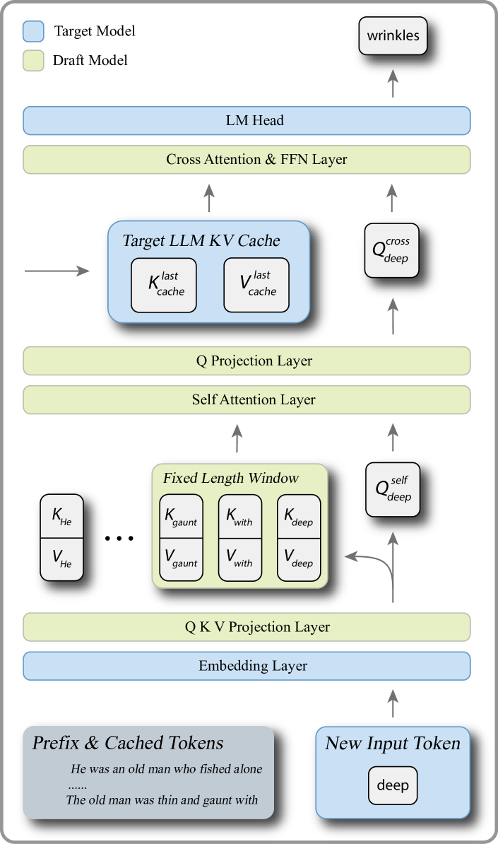
First, to alleviate the memory overhead problem, we develop a draft model architecture that circumvents the linear expansion of KV caches which maintains a constant memory footprint as the context grows. Concretely, our approach employs a sliding window self-attention component to capture local dependencies, complemented by a cache-free cross-attention module for effectively modeling long-context representations. This approach effectively mitigates memory overhead which is particularly critical in long-context inference without compromising performance.
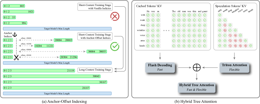
Next, to handle the training discrepancy problem, we propose the Anchor-Offset Indices to reconcile the short-context training for long-context inference. To fully train all the indices, we randomly add an offset to position indices. This ensures that some larger indices are also sufficiently trained. However, since RoPE (Su et al., 2024) is based on relative positions, directly adding an offset to all indices does not have a direct effect. Inspired by Streaming LLM (Xiao et al., 2024), we set the first four attention sink tokens as the anchor indices and only add the random offset to the remaining token index as shown in Figure 2. This indexing strategy ensures that all the indices can be sufficiently trained for the draft model. In contrast, the vanilla indexing strategy repeatedly trains only the smaller indices and is unable to train those exceeding the training set length. Meanwhile, anchoring the sink tokens ensures that the target model can approximate the attention sink patterns found in long texts, even with short texts.
Finally, to implement highly efficient tree attention, we propose a new computation method called Hybrid Tree Attention. Our insight comes from the discovery that the tree mask in tree-based speculative decoding can be decomposed into two parts, the previously cached part with a chain structure and the speculation part with a tree structure. Specifically, the tree mask is only required between the current queries and the speculation tokens (i.e., current input tokens) to ensure correctness. So we use Flash_Decoding (Dao, 2024) to compute the first part efficiently and use a custom Triton kernel fused_mask_attn to compute the second part. We then combine these components using a log-sum-exp trick, enabling our approach to accelerate tree attention computations up to 4.1 compared to previous implementations in Medusa (Cai et al., 2024).
Extensive experiments are conducted to evaluate the effectiveness of LongSpec. Experiments on five long-context understanding datasets using five LLMs as target models show that our LongSpec can effectively reduce the long-context inference latency, leading to a maximum speedup of 3.26 compared with the strong baseline model with Flash_Decoding. Additional experiments on the long reasoning task AIME24 with the o1-like model QwQ (Qwen, 2024) further validate the effectiveness of LongSpec, achieving a 2.25 speedup in wall-clock time.
2 Related Work
Speculative decoding offers a promising approach to accelerating LLMs while maintaining the quality of their outputs. Early efforts, such as Speculative Decoding (Xia et al., 2023), SpS (Leviathan et al., 2023), BiLD (Kim et al., 2024), and OSD (Liu et al., 2024c), rely on existing smaller LLMs to generate draft sequences. Some other methods aim to improve upon those early efforts (Sun et al., 2023; Miao et al., 2024; Chen et al., 2024). There are also some works using part of the target model as the draft model (Liu et al., 2024a; Zhang et al., 2024; Elhoushi et al., 2024). Retrieval-based speculative decoding methods offer an alternative by utilizing -gram matching rather than relying on smaller models. Examples include Lookahead Decoding (Fu et al., 2024), REST (He et al., 2024), and Ouroboros (Zhao et al., 2024). These approaches bypass the need for additional model training, leveraging pre-existing data patterns to construct draft sequences efficiently.
More recent advancements, including Medusa (Cai et al., 2024), EAGLE (Li et al., 2024), and GliDe (Du et al., 2024), have expanded on these foundations by designing specialized draft models and introducing tree-based speculative techniques. These methods leverage customized draft models tailored for speculative decoding, achieving higher efficiency and performance. Additionally, the tree-based approaches employed in these methods allow for more adaptive and parallelizable decoding processes, paving the way for broader applications in real-world systems.
Although speculative decoding has progressed significantly for conventional context lengths, only two existing papers focus on speculative decoding in long-context scenarios. TriForce (Sun et al., 2024) introduces a three-layer speculative decoding system that is scalable for long sequence generation. MagicDec (Chen et al., 2025) uses speculative decoding to improve both the throughput and latency of LLM inference. However, these methods mainly utilize the target model with the sparse KV cache as the draft model. The computation-intensive draft models restrict the practical usage of these methods when facing various batch sizes. In contrast, our work focuses on efficiently building a draft model with only one transformer block, achieving more effective performance across different scenarios.
3 Methodology
In this section, we present our framework LongSpec for Long-Context Speculative Decoding, which addresses three key challenges: (1) designing a lightweight draft model architecture with minimal additional memory overhead, (2) devising the training strategy with anchor-offset indices to handle long contexts effectively, and (3) implementing a fast tree attention mechanism that leverages tree-based speculation for practical usage. We detail each core component in the following subsections: Section 3.1 introduces our Memory-Efficient Architecture, Section 3.2 explains the Effective Training Regimes, and Section 3.3 describes the Fast Tree Attention implementation for inference.
3.1 Memory-Efficient Architecture
In previous work, the success of the SoTA model EAGLE depends on two factors: (1) the hidden states provided by the target model, and (2) an autoregressive structure. However, an autoregressive draft model inevitably needs to store its own KV cache, which introduces additional overhead in long-context inference requiring large GPU memory.
To avoid this extra memory overhead, we propose a draft model with constant memory usage regardless of the length of the context. As illustrated in Figure 1, our model comprises two components: the self-attention module and the following cross-attention module. The self-attention module focuses on modeling local context, while the cross-attention module captures long-context information. Because the self-attention module only processes local information, we adopt a sliding-window attention mechanism. Hence, during inference, the self-attention memory footprint does not exceed the window size, which we set to 512. We also provide the theoretical upper bound on the performance degradation caused by the slicing window in Section 3.4.
For the cross-attention component, inspired by GliDe (Du et al., 2024), we leverage the KV cache of the target model. This design not only enables better modeling of previous information but also completely removes additional storage overhead for long contexts, since the large model’s KV cache must be stored regardless of whether or not speculative decoding is employed. Different from GliDe, we also share the weights of the Embedding Layer and LM Head between the target model and the draft model, which significantly reduces the memory usage for large-vocabulary LLMs such as LLaMA.
3.2 Effective Training Regimes
Anchor-Offset Indices. With vanilla position indices, which consist of successive integers starting from , those indices appearing earlier in sequences occur more frequently than larger position indices (An et al., 2025), as shown in the Figure 2 upper left part. Consequently, larger position indices receive insufficient training updates, which leads to a training inference discrepancy. A common method to solve this problem is RoPE-based extrapolation, which trains the model with a smaller RoPE base and extends the RoPE base with interpolation for longer contexts (Gao et al., 2024; Liu et al., 2024d; Peng et al., 2024). However, directly using these methods will cause an inconsistent problem in draft model training. To leverage the target model’s KV cache, our draft model must keep the RoPE base the same as the target model. Based on our exploratory experiments, the inconsistent RoPE base between the target model and the draft model will cause a significant collapse of the cross-attention layer, which makes the draft model’s long-text capability degrade. The consistency requirement of RoPE base in the draft model limits the usage of methods like RoPE-based extrapolation, which requires flexible adjustments to the RoPE base.
Instead, we tackle this challenge by leveraging carefully designed indices. These indices must ensure that (1) the position indices in the draft model can be sufficiently trained using short-context data and (2) the indices would not cause the target model to exhibit out-of-distribution behavior because the target model shares the same indices as the draft model during training.
To satisfy these constraints, we propose the Anchor-Offset Indices strategy. Specifically, we reserve the first four positions as attention sink tokens (Xiao et al., 2024), then assign all subsequent tokens to large consecutive indices starting at a random offset (e.g., ). The anchor indices and random offset ensure that every position index can be sufficiently trained, addressing the limitation of the vanilla one that repeatedly trains only smaller indices.
Additionally, according to Xiao et al. (2024), LLM exhibits an attention sink phenomenon when dealing with long texts, which means the attention weights primarily concentrate on the first four tokens and the recent tokens. Therefore, we believe that utilizing Anchor-Offset Indices can naturally lead the target model to exhibit in-distribution behavior. In our experiments, adopting these indices in the target model only increases the loss by approximately 0.001, indicating that the target model is indeed well-suited to such changes. We also provide the theoretical upper bound of the distribution shift error in Section 3.4.
Flash Noisy Training. During training our draft model leverages the KV caches from a large model, while these KV caches are not always visible during inference. This is because the large model only updates its KV cache upon verification completion. Concretely, for the cross-attention query in the draft model, we can only guarantee access to the corresponding key-value states , satisfying , where is the number of speculative steps.
To ensure consistency between training and inference, a straightforward solution would be to add an attention mask (Du et al., 2024). However, this method is incompatible with Flash Attention (Dao et al., 2023), which would significantly degrade training speed and cause prohibitive memory overhead, particularly in long-context training scenarios. Therefore, we propose a technique called flash noisy training. During training, we randomly shift the indices of queries and key-value states with . Suppose the sequence length is , then we compute
In this way, we effectively simulate the same visibility constraints as in the inference phase, i.e., , thereby aligning the behavior at training time with the inference behavior.
3.3 Fast Tree Attention
Tree Speculative Decoding (Miao et al., 2024) leverages prefix trees and the causal structure of LLMs so that a draft model can propose multiple candidate sequences, while the target model only needs to verify them once, without altering the final results. In this process, Tree Attention plays a key role in ensuring both correctness and efficiency. Early works (Cai et al., 2024; Li et al., 2024) apply attention masks derived from prefix trees to the attention matrix, thus disabling wrong combinations between speculation tokens. However, these methods only run on PyTorch’s eager execution mode, precluding more advanced attention kernels (e.g., Flash_Decoding). As a result, the inference speed decreases significantly when the sequence length increases.
To address these performance bottlenecks, we propose a Hybrid Tree Attention mechanism, as illustrated in Figure 2. Our method is based on two key insights: 1) When performing Tree Attention, the queries and the cached key-value pairs do not require additional masks; 2) Only the queries and the key-value pairs from the current speculative tokens need masking, and the number of such speculative tokens is typically no more than 128. Based on these observations, we adopt a divide and aggregate approach that splits the attention computation into two parts and merges them afterward.
Splitting Key-Value Pairs. We partition all key-value pairs into two groups: : the cached part of the main sequence, which requires no attention mask; and : the speculative-stage part, which needs attention masks. For , we invoke the efficient Flash_Decoding kernel. For , we use our custom Triton kernel fused_mask_attn, which applies blockwise loading and masking in the KV dimension, enabling fast computation of attention. This step yields two sets of attention outputs along with their corresponding denominators (i.e., log-sum-exp of all attention scores) .
Aggregation. We then combine these two parts into the final attention output via a log-sum-exp trick. First, we compute
and then apply a weighted summation to the two outputs:
The theoretical guarantee is provided in Appendix A. As outlined above, this hybrid approach employs the highly efficient Flash_Decoding kernel for most of the computations in long-sequence inference and only uses a custom masking attention fused_mask_attn for the small number of speculative tokens. The kernel fused_mask_attn follows the design philosophy of Flash Attention 2 (Dao et al., 2023) by splitting , , and into small blocks. This strategy reduces global memory I/O and fully leverages GPU streaming multiprocessors. Furthermore, for each block in the computation of , the mask matrix is loaded and used to apply the masking operation. The Hybrid Tree Attention effectively balances the parallel verification of multiple branches with improved inference speed, all without compromising the correctness.
3.4 Theoretical Analysis
Here we would like to provide the theoretical analysis of our method. Before the statement of our results, we would like to define some quantities. First, for the memory-efficient architecture, we denote the sum of the attention score outside the window as , which should be small due to the locality of the language. Second, for our index offset technique, we denote the distribution of the offset as . In addition, we denote the true distribution of the index of the first token in the window as . Finally, we assume that the GliDe function is trained on i.i.d. samples, and the Frobenius norms of all the parameters are upper bounded by .
Theorem 3.1 (Informal).
Under regularity assumptions, the inference error between the Maximum Likelihood Estimate (MLE) trained by our method and the optimal GliDe parameter that take all tokens as inputs is upper bounded by
with probability at least . Here the approximation error is , the distribution shift error is , and the generalization error is .
The formal statement and the proof are provided in Appendix D. The approximation error results from that we adopt a sliding window instead of using all tokens. This error is proportional to the attention score outside the window. The distribution shift error results from the positional embedding distributional shift. In our experiments, we set as the uniform distribution, which will have a smaller distribution shift than not adopting this position offset technique. The generalization error results from that we use samples to train the model.
| Setting | GovReport | QMSum | Multi-News | LCC | RepoBench-P | |||||||||||
| Tokens/s | Speedup | Tokens/s | Speedup | Tokens/s | Speedup | Tokens/s | Speedup | Tokens/s | Speedup | |||||||
|
V-7B |
Vanilla HF | 1.00 | 25.25 | - | 1.00 | 18.12 | - | 1.00 | 27.29 | - | 1.00 | 25.25 | - | 1.00 | 19.18 | - |
| Vanilla FA | 1.00 | 45.76 | 1.00 | 1.00 | 43.68 | 1.00 | 1.00 | 55.99 | 1.00 | 1.00 | 54.07 | 1.00 | 1.00 | 46.61 | 1.00 | |
| MagicDec | 2.23 | 41.68 | 0.91 | 2.29 | 42.91 | 0.98 | 2.31 | 44.82 | 0.80 | 2.52 | 46.96 | 0.87 | 2.57 | 48.75 | 1.05 | |
| LongSpec | 3.57 | 102.23 | 2.23 | 3.14 | 88.87 | 2.04 | 3.51 | 100.55 | 1.80 | 3.73 | 107.30 | 1.99 | 3.86 | 110.76 | 2.38 | |
|
V-13B |
Vanilla HF | 1.00 | 17.25 | - | 1.00 | 11.86 | - | 1.00 | 18.81 | - | 1.00 | 17.25 | - | 1.00 | 13.44 | - |
| Vanilla FA | 1.00 | 28.52 | 1.00 | 1.00 | 27.43 | 1.00 | 1.00 | 35.01 | 1.00 | 1.00 | 33.87 | 1.00 | 1.00 | 29.14 | 1.00 | |
| MagicDec | 2.95 | 38.24 | 1.34 | 2.87 | 37.15 | 1.35 | 2.97 | 39.47 | 1.13 | 2.96 | 38.40 | 1.13 | 2.94 | 36.66 | 1.26 | |
| LongSpec | 3.31 | 71.08 | 2.49 | 2.76 | 57.15 | 2.08 | 3.44 | 78.20 | 2.23 | 3.57 | 81.00 | 2.39 | 3.59 | 77.22 | 2.65 | |
|
LC-7B |
Vanilla HF | 1.00 | 25.27 | - | 1.00 | 14.11 | - | 1.00 | 27.66 | - | 1.00 | 25.27 | - | 1.00 | 17.02 | - |
| Vanilla FA | 1.00 | 42.14 | 1.00 | 1.00 | 36.87 | 1.00 | 1.00 | 50.19 | 1.00 | 1.00 | 54.17 | 1.00 | 1.00 | 42.69 | 1.00 | |
| MagicDec | 2.26 | 41.90 | 0.99 | 2.20 | 40.82 | 1.11 | 2.32 | 43.94 | 0.88 | 2.77 | 51.73 | 0.96 | 2.57 | 44.13 | 1.03 | |
| LongSpec | 3.59 | 101.43 | 2.41 | 3.06 | 85.23 | 2.31 | 3.41 | 97.93 | 1.95 | 4.21 | 122.30 | 2.26 | 4.03 | 115.27 | 2.70 | |
|
LC-13B |
Vanilla HF | 1.00 | 17.72 | - | 1.00 | 12.08 | - | 1.00 | 18.74 | - | 1.00 | 17.72 | - | 1.00 | 13.85 | - |
| Vanilla FA | 1.00 | 28.56 | 1.00 | 1.00 | 27.18 | 1.00 | 1.00 | 35.37 | 1.00 | 1.00 | 34.58 | 1.00 | 1.00 | 29.74 | 1.00 | |
| MagicDec | 2.40 | 31.37 | 1.10 | 2.38 | 30.84 | 1.13 | 2.43 | 32.58 | 0.92 | 2.68 | 35.77 | 1.03 | 2.85 | 35.67 | 1.20 | |
| LongSpec | 3.58 | 76.26 | 2.67 | 3.15 | 64.41 | 2.37 | 3.50 | 80.48 | 2.28 | 4.01 | 90.92 | 2.63 | 4.46 | 96.96 | 3.26 | |
|
L-8B |
Vanilla HF | 1.00 | 21.59 | - | 1.00 | 18.67 | - | 1.00 | 29.91 | - | 1.00 | 29.48 | - | 1.00 | 22.77 | - |
| Vanilla FA | 1.00 | 53.14 | 1.00 | 1.00 | 51.22 | 1.00 | 1.00 | 56.94 | 1.00 | 1.00 | 56.73 | 1.00 | 1.00 | 54.08 | 1.00 | |
| MagicDec | 2.04 | 36.14 | 0.68 | 2.00 | 35.78 | 0.70 | 2.33 | 39.57 | 0.70 | 2.65 | 46.95 | 0.83 | 2.61 | 44.39 | 0.82 | |
| LongSpec | 3.25 | 84.57 | 1.59 | 2.99 | 75.68 | 1.48 | 3.36 | 91.11 | 1.60 | 3.28 | 89.33 | 1.57 | 3.39 | 91.28 | 1.69 | |
4 Experiments
4.1 Settings
Target and draft models. We select four widely-used long-context LLMs, Vicuna (including 7B and 13B) (Chiang et al., 2023), LongChat (including 7B and 13B) (Li et al., 2023), LLaMA-3.1-8B-Instruct (Dubey et al., 2024), and QwQ-32B (Qwen, 2024), as target models. In order to make the draft model and target model more compatible, our draft model is consistent with the target model in various parameters such as the number of KV heads.
Training Process. We first train our draft model with Achor-Offest Indices on the SlimPajama-6B pretraining dataset (Soboleva et al., 2023). The random offset is set as a random integer from 0 to 15k for Vicuna models and LongChat-7B, and 0 to 30k for the other three models because they have longer maximum context length. Then we train our model on a small subset of the Prolong-64k long-context dataset (Gao et al., 2024) in order to gain the ability to handle long texts. Finally, we finetune our model on a self-built long-context supervised-finetuning (SFT) dataset to further improve the model performance. The position index of the last two stages is the vanilla indexing policy because the training data is sufficiently long. We apply flash noisy training during all three stages to mitigate the training and inference inconsistency, the extra overhead of flash noisy training is negligible. Standard cross-entropy is used to optimize the draft model while the parameters of the target model are kept frozen. To mitigate the VRAM peak caused by the computation of the logits, we use a fused-linear-and-cross-entropy loss implemented by the Liger Kernel (Hsu et al., 2024), which computes the LM head and the softmax function together and can greatly alleviate this problem. More details on model training can be found in Appendix B.
Test Benchmarks. We select tasks from the LongBench benchmark (Bai et al., 2024) that involve generating longer outputs, because tasks with shorter outputs, such as document-QA, make it challenging to measure the speedup ratio fairly with speculative decoding. Specifically, we focus on long-document summarization and code completion tasks and conduct tests on five datasets: GovReport (Huang et al., 2021), QMSum (Zhong et al., 2021), Multi-News (Fabbri et al., 2019), LCC (Guo et al., 2023), and RepoBench-P (Liu et al., 2024b). We test QwQ-32B on the famous reasoning dataset AIME24 (Numina, 2024).
We compare our method with the original target model and MagicDec, a simple prototype of TriForce. To highlight the significance of Flash_Decoding in long-context scenarios, we also present the performance of the original target model using both eager attention implemented by Huggingface and Flash_Decoding for comparison. To make a fair comparison, we also use Flash_Decoding for baseline MagicDec. The most important metric for speculative decoding is the walltime speedup ratio, which is the actual test speedup ratio relative to vanilla autoregressive decoding. We also test the average acceptance length , i.e., the average number of tokens accepted per forward pass of the target LLM.
4.2 Main Results
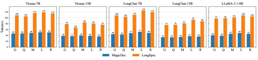
Table 1 and Figure 3 show the decoding speeds and mean accept lengths across the five evaluated datasets at and respectively. Our proposed method significantly outperforms all other approaches on both summarization tasks and code completion tasks. When , on summarization tasks, our method can achieve a mean accepted length of around 3.5 and a speedup of up to 2.67; and on code completion tasks, our method can achieve a mean accepted length of around 4 and a speedup of up to 3.26. This highlights the robustness and generalizability of our speculative decoding approach, particularly in long-text generation tasks. At , our method’s performance achieves around 2.5 speedup, maintaining a substantial lead over MagicDec. This indicates that our approach is robust across different temperature settings, further validating its soundness and efficiency.
While MagicDec demonstrates competitive acceptance rates with LongSpec, its speedup is noticeably lower in our experiments. This is because MagicDec is primarily designed for scenarios with large batch sizes and tensor parallelism. In low-batch-size settings, its draft model leverages all parameters of the target model with sparse KV Cache becomes excessively heavy. This design choice leads to inefficiencies, as the draft model’s computational overhead outweighs its speculative benefits. Our results reveal that MagicDec only achieves acceleration ratios on partial datasets when using a guess length and consistently exhibits negative acceleration around 0.7 when , further underscoring the limitations of this method in such configurations.
Lastly, we can find attention implementation plays a critical role in long-context speculative decoding performance. In our experiments, “Vanilla HF” refers to HuggingFace’s attention implementation, while “Vanilla FA” employs Flash_Decoding. The latter demonstrates nearly a speedup over the former, even as a standalone component, and our method can achieve up to speedup over HF Attention on code completion datasets. This result underscores the necessity for speculative decoding methods to be compatible with optimized attention mechanisms like Flash_Decoding, especially in long-text settings. Our hybrid tree attention approach achieves this compatibility, allowing us to fully leverage the advantages of Flash_Decoding and further speedup.
4.3 Ablation Studies
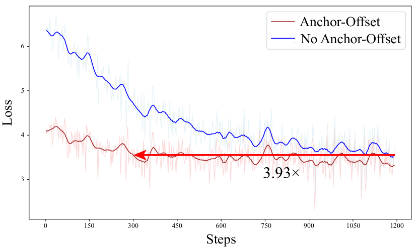
Anchor-Offset Indices. The experimental results demonstrate the significant benefits of incorporating the Anchor-Offset Indices. Figure 4 shows that pretrained with Anchor-Offset Indices achieve a lower initial loss and final loss compared to those trained without it when training over the real long-context dataset. Notably, the initalization with Anchor-Offset Indices reaches the same loss level faster than its counterpart. Table 2 further highlights the performance improvements across two datasets, a summary dataset Multi-News, and a code completion dataset RepoBench-P. Models with Anchor-Offset Indices exhibit faster output speed and larger average acceptance length . These results underscore the effectiveness of Anchor-Offset Indices in enhancing both training efficiency and model performance.
| Multi-News | RepoBench-P | |||
| Tokens/s | Tokens/s | |||
| w/o Anchor-Offset | 3.20 | 85.98 | 3.26 | 85.21 |
| w/ Anchor-Offset | 3.36 | 91.11 | 3.39 | 91.28 |
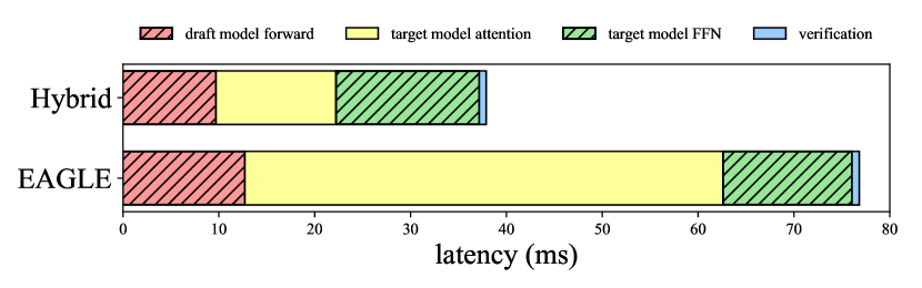
Hybrid Tree Attention. The results presented in Figure 5 highlight the effectiveness of the proposed Hybrid Tree Attention, which combines Flash_Decoding with the Triton kernel fused_mask_attn. While the time spent on the draft model forward pass and the target model FFN computations remain comparable across the two methods, the hybrid approach exhibits a significant reduction in latency for the target model’s attention layer (the yellow part). Specifically, the attention computation latency decreases from 49.92 ms in the HF implementation to 12.54 ms in the hybrid approach, resulting in an approximately 75% improvement. The verification step time difference is minimal, further solidifying the conclusion that the primary performance gains stem from optimizing the attention mechanism.
4.4 Long CoT Acceleration
Long Chain-of-Thought (LongCoT) tasks have gained significant attention recently due to their ability to enable models to perform complex reasoning and problem-solving over extended outputs (Qwen, 2024; OpenAI, 2024). In these tasks, while the prefix input is often relatively short, the generated output can be extremely long, posing unique challenges in terms of efficiency and token acceptance. Our method is particularly well-suited for addressing these challenges, effectively handling scenarios with long outputs. It is worth mentioning that MagicDec is not suitable for such long-output scenarios because the initial inference stage of the LongCoT task is not the same as the traditional long-context task. In LongCoT tasks, where the prefix is relatively short, the draft model in MagicDec will completely degrade into the target model, failing to achieve acceleration.
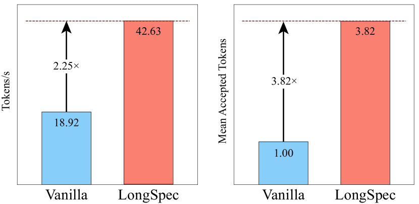
We evaluate our method on the QwQ-32B model using the widely-used benchmark AIME24 dataset, with a maximum output length set to 32k tokens. The results, illustrated in Figure 6, demonstrate a significant improvement in both generation speed and mean accepted tokens. Specifically, our method achieved a generation rate of 42.63 tokens/s, 2.25 higher than the baseline’s 18.92 tokens/s, and an average of 3.82 mean accepted tokens. Notably, QwQ-32B with LongSpec achieves even lower latency than the vanilla 7B model with Flash_Decoding, demonstrating that our method effectively accelerates the LongCoT model. These findings not only highlight the effectiveness of our method in the LongCoT task but also provide new insights into lossless inference acceleration for the o1-like model. We believe that speculative decoding will play a crucial role in accelerating this type of model in the future.
4.5 Throughput
The throughput results of Vicuna-7B on the RepoBench-P dataset show that LongSpec consistently outperforms both Vanilla and MagicDec across all batch sizes. At a batch size of 8, LongSpec achieves a throughput of 561.32 tokens/s, approximately 1.8 higher than MagicDec (310.58 tokens/s) and nearly 2 higher than Vanilla (286.96 tokens/s). MagicDec, designed with throughput optimization in mind, surpasses Vanilla as the batch size increases, reflecting its targeted improvements. However, LongSpec still sustains its advantage, maintaining superior throughput across all tested batch sizes.
5 Conclusion
In this paper, we propose LongSpec, a novel framework designed to enhance speculative decoding for long-context scenarios. Unlike previous speculative decoding methods that primarily focus on short-context settings, LongSpec directly addresses three key challenges: excessive memory overhead, inadequate training for large position indices, and inefficient tree attention computation. To mitigate memory constraints, we introduce an efficient draft model architecture that maintains a constant memory footprint by leveraging a combination of sliding window self-attention and cache-free cross-attention. To resolve the training limitations associated with short context data, we propose the Anchor-Offset Indices, ensuring that large positional indices are sufficiently trained even within short-sequence datasets. Finally, we introduce Hybrid Tree Attention, which efficiently integrates tree-based speculative decoding with Flash_Decoding. Extensive experiments demonstrate the effectiveness of LongSpec in long-context understanding tasks and real-world long reasoning tasks. Our findings highlight the importance of designing speculative decoding methods specifically tailored for long-context settings and pave the way for future research in efficient large-scale language model inference.
Impact Statements
This paper presents work whose goal is to advance the field of Machine Learning. There are many potential societal consequences of our work, none which we feel must be specifically highlighted here.
References
- Achiam et al. (2023) Achiam, J., Adler, S., Agarwal, S., Ahmad, L., Akkaya, I., Aleman, F. L., Almeida, D., Altenschmidt, J., Altman, S., Anadkat, S., et al. GPT-4 technical report. arXiv preprint arXiv:2303.08774, 2023.
- An et al. (2025) An, C., Zhang, J., Zhong, M., Li, L., Gong, S., Luo, Y., Xu, J., and Kong, L. Why does the effective context length of llms fall short? In Proceedings of the International Conference on Learning Representations, 2025.
- Bai et al. (2024) Bai, Y., Lv, X., Zhang, J., Lyu, H., Tang, J., Huang, Z., Du, Z., Liu, X., Zeng, A., Hou, L., Dong, Y., Tang, J., and Li, J. LongBench: A bilingual, multitask benchmark for long context understanding. In Proceedings of the 62nd Annual Meeting of the Association for Computational Linguistics, 2024.
- Cai et al. (2024) Cai, T., Li, Y., Geng, Z., Peng, H., Lee, J. D., Chen, D., and Dao, T. Medusa: Simple LLM inference acceleration framework with multiple decoding heads. In Proceedings of the International Conference on Machine Learning, 2024.
- Chen et al. (2025) Chen, J., Tiwari, V., Sadhukhan, R., Chen, Z., Shi, J., Yen, I. E.-H., and Chen, B. MagicDec: Breaking the latency-throughput tradeoff for long context generation with speculative decoding. In Proceedings of the International Conference on Learning Representations, 2025.
- Chen et al. (2024) Chen, Z., Yang, X., Lin, J., Sun, C., Chang, K., and Huang, J. Cascade speculative drafting for even faster LLM inference. In Advances in Neural Information Processing Systems, 2024.
- Chiang et al. (2023) Chiang, W.-L., Li, Z., Lin, Z., Sheng, Y., Wu, Z., Zhang, H., Zheng, L., Zhuang, S., Zhuang, Y., Gonzalez, J. E., et al. Vicuna: An open-source chatbot impressing GPT-4 with 90% ChatGPT quality, 2023. URL https://vicuna.lmsys.org.
- Dao (2024) Dao, T. FlashAttention-2: Faster attention with better parallelism and work partitioning. In Proceedings of the International Conference on Learning Representations, 2024.
- Dao et al. (2023) Dao, T., Haziza, D., Massa, F., and Sizov, G. Flash-Decoding for long-context inference, 2023. URL https://crfm.stanford.edu/2023/10/12/flashdecoding.html.
- Deepseek (2024) Deepseek. Deepseek’s api context caching on disk technology, 2024. URL https://api-docs.deepseek.com/guides/kv_cache.
- Du et al. (2024) Du, C., Jiang, J., Yuanchen, X., Wu, J., Yu, S., Li, Y., Li, S., Xu, K., Nie, L., Tu, Z., and You, Y. Glide with a cape: A low-hassle method to accelerate speculative decoding. In Proceedings of the International Conference on Machine Learning, 2024.
- Dubey et al. (2024) Dubey, A., Jauhri, A., Pandey, A., Kadian, A., Al-Dahle, A., Letman, A., Mathur, A., Schelten, A., Yang, A., Fan, A., et al. The llama 3 herd of models. arXiv preprint arXiv:2407.21783, 2024.
- Elhoushi et al. (2024) Elhoushi, M., Shrivastava, A., Liskovich, D., Hosmer, B., Wasti, B., Lai, L., Mahmoud, A., Acun, B., Agarwal, S., Roman, A., Aly, A., Chen, B., and Wu, C.-J. LayerSkip: Enabling early exit inference and self-speculative decoding. In Proceedings of the 62nd Annual Meeting of the Association for Computational Linguistics, 2024.
- Fabbri et al. (2019) Fabbri, A. R., Li, I., She, T., Li, S., and Radev, D. Multi-News: A large-scale multi-document summarization dataset and abstractive hierarchical model. In Proceedings of the 57th Annual Meeting of the Association for Computational Linguistics, 2019.
- Fu et al. (2024) Fu, Y., Bailis, P., Stoica, I., and Zhang, H. Break the sequential dependency of LLM inference using lookahead decoding. In Proceedings of the International Conference on Machine Learning, 2024.
- Gao et al. (2024) Gao, T., Wettig, A., Yen, H., and Chen, D. How to train long-context language models (effectively). arXiv preprint arXiv:2410.02660, 2024.
- Google (2024) Google. Gemini API context caching feature, 2024. URL https://ai.google.dev/gemini-api/docs/caching.
- Guo et al. (2023) Guo, D., Xu, C., Duan, N., Yin, J., and McAuley, J. Longcoder: A long-range pre-trained language model for code completion. In Proceedings of the International Conference on Machine Learning, 2023.
- He et al. (2024) He, Z., Zhong, Z., Cai, T., Lee, J., and He, D. REST: Retrieval-based speculative decoding. In Proceedings of the Conference of the North American Chapter of the Association for Computational Linguistics, 2024.
- Hsu et al. (2024) Hsu, P.-L., Dai, Y., Kothapalli, V., Song, Q., Tang, S., Zhu, S., Shimizu, S., Sahni, S., Ning, H., and Chen, Y. Liger kernel: Efficient triton kernels for LLM training. arXiv preprint arXiv:2410.10989, 2024.
- Huang et al. (2021) Huang, L., Cao, S., Parulian, N., Ji, H., and Wang, L. Efficient attentions for long document summarization. In Proceedings of the Conference of the North American Chapter of the Association for Computational Linguistics, 2021.
- Kim et al. (2024) Kim, S., Mangalam, K., Moon, S., Malik, J., Mahoney, M. W., Gholami, A., and Keutzer, K. Speculative decoding with big little decoder. In Advances in Neural Information Processing Systems, 2024.
- Kingma & Ba (2015) Kingma, D. P. and Ba, J. L. Adam: A method for stochastic gradient descent. In Proceedings of the International Conference on Learning Representations, 2015.
- Leviathan et al. (2023) Leviathan, Y., Kalman, M., and Matias, Y. Fast inference from transformers via speculative decoding. In Proceedings of the International Conference on Machine Learning, 2023.
- Li et al. (2023) Li, D., Shao, R., Xie, A., Sheng, Y., Zheng, L., Gonzalez, J. E., Stoica, I., Ma, X., and Zhang, H. How long can open-source llms truly promise on context length?, 2023. URL https://lmsys.org/blog/2023-06-29-longchat.
- Li et al. (2024) Li, Y., Wei, F., Zhang, C., and Zhang, H. Eagle: Speculative sampling requires rethinking feature uncertainty. In Proceedings of the International Conference on Machine Learning, 2024.
- Liu et al. (2024a) Liu, F., Tang, Y., Liu, Z., Ni, Y., Tang, D., Han, K., and Wang, Y. Kangaroo: Lossless self-speculative decoding for accelerating LLMs via double early exiting. In Advances in Neural Information Processing Systems, 2024a.
- Liu et al. (2024b) Liu, T., Xu, C., and McAuley, J. RepoBench: Benchmarking repository-level code auto-completion systems. In Proceedings of the International Conference on Learning Representations, 2024b.
- Liu et al. (2024c) Liu, X., Hu, L., Bailis, P., Cheung, A., Deng, Z., Stoica, I., and Zhang, H. Online speculative decoding. In Proceedings of the International Conference on Machine Learning, 2024c.
- Liu et al. (2024d) Liu, X., Yan, H., An, C., Qiu, X., and Lin, D. Scaling laws of roPE-based extrapolation. In Proceedings of the International Conference on Learning Representations, 2024d.
- Loshchilov & Hutter (2017) Loshchilov, I. and Hutter, F. SGDR: Stochastic gradient descent with warm restarts. In Proceedings of the International Conference on Learning Representations, 2017.
- Miao et al. (2024) Miao, X., Oliaro, G., Zhang, Z., Cheng, X., Wang, Z., Zhang, Z., Wong, R. Y. Y., Zhu, A., Yang, L., Shi, X., Shi, C., Chen, Z., Arfeen, D., Abhyankar, R., and Jia, Z. Specinfer: Accelerating large language model serving with tree-based speculative inference and verification. In Proceedings of the 29th ACM International Conference on Architectural Support for Programming Languages and Operating Systems, 2024.
- Numina (2024) Numina, P. AIMO validation AIME, 2024. URL https://huggingface.co/datasets/AI-MO/aimo-validation-aime.
- OpenAI (2024) OpenAI. Learning to reason with llms, September 2024. URL https://openai.com/index/learning-to-reason-with-llms/.
- Peng et al. (2024) Peng, B., Quesnelle, J., Fan, H., and Shippole, E. YaRN: Efficient context window extension of large language models. In Proceedings of the International Conference on Learning Representations, 2024.
- Qwen (2024) Qwen. QwQ: Reflect deeply on the boundaries of the unknown, November 2024. URL https://qwenlm.github.io/blog/qwq-32b-preview/.
- Rasley et al. (2020) Rasley, J., Rajbhandari, S., Ruwase, O., and He, Y. Deepspeed: System optimizations enable training deep learning models with over 100 billion parameters. In Proceedings of the 26th ACM SIGKDD International Conference on Knowledge Discovery and Data Mining, 2020.
- Soboleva et al. (2023) Soboleva, D., Al-Khateeb, F., Myers, R., Steeves, J. R., Hestness, J., and Dey, N. SlimPajama: A 627b token cleaned and deduplicated version of redpajama, 2023. URL https://huggingface.co/datasets/cerebras/SlimPajama-627B.
- Su et al. (2024) Su, J., Ahmed, M., Lu, Y., Pan, S., Bo, W., and Liu, Y. Roformer: Enhanced transformer with rotary position embedding. Neurocomputing, 2024.
- Sun et al. (2024) Sun, H., Chen, Z., Yang, X., Tian, Y., and Chen, B. TriForce: Lossless acceleration of long sequence generation with hierarchical speculative decoding. In Proceedings of the First Conference on Language Modeling, 2024.
- Sun et al. (2023) Sun, Z., Suresh, A. T., Ro, J. H., Beirami, A., Jain, H., and Yu, F. X. Spectr: Fast speculative decoding via optimal transport. In Advances in Neural Information Processing Systems, 2023.
- Xia et al. (2023) Xia, H., Ge, T., Wang, P., Chen, S.-Q., Wei, F., and Sui, Z. Speculative decoding: Exploiting speculative execution for accelerating seq2seq generation. In Findings of the Association for Computational Linguistics: EMNLP 2023, 2023.
- Xiao et al. (2024) Xiao, G., Tian, Y., Chen, B., Han, S., and Lewis, M. Efficient streaming language models with attention sinks. In Proceedings of the International Conference on Learning Representations, 2024.
- Zhang et al. (2022) Zhang, F., Liu, B., Wang, K., Tan, V., Yang, Z., and Wang, Z. Relational reasoning via set transformers: Provable efficiency and applications to marl. Advances in Neural Information Processing Systems, 35:35825–35838, 2022.
- Zhang et al. (2024) Zhang, J., Wang, J., Li, H., Shou, L., Chen, K., Chen, G., and Mehrotra, S. Draft& verify: Lossless large language model acceleration via self-speculative decoding. In Proceedings of the 62nd Annual Meeting of the Association for Computational Linguistics, 2024.
- Zhang et al. (2023) Zhang, Y., Zhang, F., Yang, Z., and Wang, Z. What and how does in-context learning learn? Bayesian model averaging, parameterization, and generalization. arXiv preprint arXiv:2305.19420, 2023.
- Zhao et al. (2024) Zhao, W., Huang, Y., Han, X., Xu, W., Xiao, C., Zhang, X., Fang, Y., Zhang, K., Liu, Z., and Sun, M. Ouroboros: Generating longer drafts phrase by phrase for faster speculative decoding. In Proceedings of the Conference on Empirical Methods in Natural Language Processing, 2024.
- Zhong et al. (2021) Zhong, M., Yin, D., Yu, T., Zaidi, A., Mutuma, M., Jha, R., Hassan, A., Celikyilmaz, A., Liu, Y., Qiu, X., et al. QMSum: A new benchmark for query-based multi-domain meeting summarization. In Proceedings of the Conference of the North American Chapter of the Association for Computational Linguistics, 2021.
Appendix A Correctness for Attention Aggregation
Because the query matrix can be decomposed into several rows, each representing a separate query , we can only consider the output of each row’s after calculating attention with KV. In this way, we can assume that the KV involved in the calculation has undergone the tree mask, which can simplify our proof. We only need to prove that the output obtained from each individual meets the requirements, which can indicate that the overall output of the entire matrix also meets the requirements.
Proposition A.1.
Denote the log-sum-exp of the merged attention as follows:
Then we can write the merged attention output in the following way:
Proof.
A standard scaled dot-product attention for (of size ) attending to and (together of size and respectively) can be written as:
Because and are formed by stacking and , we split the logit matrix accordingly:
Denote these sub-logit matrices as:
Each row of corresponds to the dot products between the -th query in and all rows in , while rows of correspond to the same query but with .
In order to combine partial attentions, we keep track of the log of the sum of exponentials of each sub-logit set. Concretely, define:
| (1) |
where denotes the logit for the -th element, and similarly for .
Then and can be written as:
| (2) |
And the whole attention score can be written as:
| (3) |
| (4) |
∎
Appendix B Experiments Details
All models are trained using eight A100 80GB GPUs. For the 7B, 8B, and 13B target models trained on short-context data, we employ LongSpec with ZeRO-1 (Rasley et al., 2020). For the 7B, 8B, and 13B models trained on long-context data, as well as for all settings of the 33B target models, we utilize ZeRO-3.
For the SlimPajama-6B dataset, we configure the batch size (including accumulation) to 2048, set the maximum learning rate to 5e-4 with a cosine learning rate schedule (Loshchilov & Hutter, 2017), and optimize the draft model using AdamW (Kingma & Ba, 2015). When training on long-context datasets, we adopt a batch size of 256 and a maximum learning rate of 5e-6. The draft model is trained for only one epoch on all datasets.
It is important to note that the primary computational cost arises from forwarding the target model to obtain the KV cache. Recently, some companies have introduced a service known as context caching (Deepseek, 2024; Google, 2024), which involves storing large volumes of KV cache. Consequently, in real-world deployment, these pre-stored KV caches can be directly utilized as training data, significantly accelerating the training process.
For the tree decoding of LongSpec, we employ dynamic beam search to construct the tree. Previous studies have shown that beam search, while achieving high acceptance rates, suffers from slow processing speed in speculative decoding (Du et al., 2024). Our research identifies that this slowdown is primarily caused by KV cache movement. In traditional beam search, nodes that do not fall within the top- likelihood are discarded, a step that necessitates KV cache movement. However, in speculative decoding, discarding these nodes is unnecessary, as draft sequences are not required to maintain uniform lengths. Instead, we can simply halt the computation of descendant nodes for low-likelihood branches without removing them entirely. By adopting this approach, beam search attains strong performance without excessive computational overhead. In our experiments, the beam width is set to for each speculation step. All inference experiments in this study are conducted using float16 precision on a single A100 80GB GPU.
Appendix C Notation
For a positive integer , we define the set . For a vector , we adopt to denote the norm of vectors. For a matrix , where for , we define the -norm of as The Frobenius norm is denoted as . We write to mean for an absolute constant .
Appendix D Theoretical Analysis
In this section, we provide the theoretical analysis of our methods. We begin with the definition of our Glide network. It consists of three modules: the self-attention module, the cross-attention module, and the Feed-Forward (FF) module. Here the self-attention and the cross-attention are both based on the attention module. For a query and KV pairs , the attention module calculate the output as
| (5) |
where is the softmax operator, are the weight matrices, is the rotary positional embedding function that appiles RoPE on inputs, and is the row-wise normalization of the input, which is defined as
Compared to the implementation of attention in PyTorch, we merge the weight matrix into here for ease of notation. Our results can be easily generalized to the formulation that explicitly parameterizes . The Multi-Head Attention (MHA) with heads is the combination of attention, i.e.,
| (6) |
where are the weights of all the attention heads. The self attention module generates the output for a query according to the KV pairs that include and other tokens, i.e., are defined as
where for are the input vectors prior to . In contrast, the cross-attention generates outputs for according to the KV pairs that excludes , i.e., . The FF module process an input vector as
| (7) |
where are weights of FF module, and is an element-wise activation function. For example, the activation function can be ReLU and sigmoid. In the following, we will omit the parameters of each module for ease of notation. The Glide function, denoted as , is defined as
| (8) |
where is the embeddings of all the tokens prior to , are the hidden states of large models, is the unembedding matrix ( is the alphabet size of the tokens), and denotes the parameters of all these three modules and , i.e.,
Here the superscripts and denote the index of the layer. We denote all the plausible parameter configurations as as
In the following, we would like to study the error analysis of our method. In fact, we need to define a variant of this function, which contains two modifications. The first modification is the positional embedding. Instead of using the positional embeddings corresponding to the continuous positions, we offset the positions of the tokens with position index larger than jointly to . We denote such positional embedding with . The corresponding is denoted as . Here we note that , i.e., there is no position offset in the original attention module. The second modification is that we truncate to a sliding window, which is detailed discussed in Section 3.1. We denote the truncated version of as . Then our proposed training method is to train the following function
| (9) |
We assume that the glide function is trained on a dataset with i.i.d. samples of a distribution , i.e., , where is the vocabulary index of true next token for -th sample. During the training process, the position offsets are i.i.d. samples of a distribution . Then we define the Maximum Likelihood Estimate (MLE) as
where denotes the expectation with respect to the empirical distribution induced by , and is the distribution of the position offset. After the training process, we will inference according to the following function
i.e., we do not delibrately shfit the token positions in the inference. To analyze the performance loss due to our method, we then define the optimal parameters of the original Glide function. Here optimality means that we have infinite number of training data points, i.e., the expectation is taken with respect to the true distribution instead of the empirical distribution induced by the dataset.
Assumption D.1 (Concentration of Window Attention Score).
For any on the support of and the optimal parameter , the sum of the attention scores of the tokens in that are not included in is upper bounded by at the first layer.
Intuitively, we note that this assumption largely holds when the answer for the query is included in the window we use. It means that the glide function does not need to gather information outside the window.
Assumption D.2 (Boundness of Inputs).
For any on the support of , we have that , , and .
This assumption always holds in the realistic setting, since all the inputs are stored in the computer, which can only represent finite numbers. For the prompt distribution , we denote the distribution of the position index of the starting token in the window as .
Assumption D.3.
The content in the window is independent of its starting index for distribution .
This assumption states that the contents and its absolute position in the context are independent. This generally holds in the long context, since the position of a sentence can hardly imply the content of this sentence in the long context.
Theorem D.4.
Here we can see that the error consists of three components. The first one results from that we adopt a sliding window instead of using all tokens. This error is proportional to the attention score outside the window. The second one results from the positinoal embedding distributional shift. In our experiments, we set as the uniform distribution, which will have smaller distribution shift than not adopting this position offse technique. The last term results from that we use samples to train the model.
Proof of Theorem D.4.
The proof takes three steps.
-
•
Decompose the performance error.
-
•
Bound each term in the decomposition.
-
•
Conclude the proof.
Step 1: Decompose the performance error.
Before the detailed decomposition, we would like to define optimal parameters of the modified Glide function as follows.
where is the optimal parameter that considers both the position offse and inputs truncation, and is the optimal parameter that only consider the input truncation.
| (10) |
where the inequality follows from the fact that all the optimization error is less and equal to according to the definitions.
Step 2: Bound each term in the decomposition.
Then we would like to separately upper bound the three kinds of error derived in the first step. Before calculating the upper bounds, we note that for any due to Lemma E.3. For the approximation error, we have that
where the first inequality results from the definition of , and the second inequality results from Lemmas E.2 and E.1. For the positional embedding distribution shift, we have that
where the inequality results from the definition of the total variation. For the generalization error, we would like to apply Theorem 4.3 of (Zhang et al., 2023). In fact, we have that with probability at least , the following inequality holds.
Step 3: Conclude the proof.
Combining all the results in steps 1 and 2, we have that
∎
Appendix E Supporting Lemmas
Proposition E.1 (Proposition 11.1 in (Zhang et al., 2023)).
For any , , and , we have that
Lemma E.2 (Lemma I.8 in (Zhang et al., 2023)).
For any , and any for , if , , , for , then we have
Lemma E.3 (Lemma 17 in (Zhang et al., 2022) ).
Given any two conjugate numbers , i.e., , and , for any and , we have
Lemma E.4.
For a query vector , and two sets of key-value pairs , , , and , We define attention scores and as
Then we have that
Appendix F Case Study
Here we display some illustrative cases from GovReport, where tokens marked in blue indicate draft tokens accepted by the target model.