Entanglement fidelity of Petz decoder for one-shot entanglement transmission
Abstract
One-shot entanglement transmission is a quantum information processing task where a quantum state is sent to a second party over a noisy channel. The goal of the task is to approximately recover the original state by applying a decoder to the output of the noisy channel. In this work, we note that the Petz map induces a universal decoder for one-shot entanglement transmission, and we quantify its entanglement fidelity. This fidelity is found to be determined by the singly minimized Petz Rényi mutual information of order associated with a complementary channel, thus providing an operational interpretation of this information measure. Furthermore, we compare the performance of this decoder to that of the decoder induced by the twirled Petz map and the Schumacher-Westmoreland decoder.
1 Introduction
Faithful transmission of quantum information between various parties is essential for quantum computation and communication. The analysis of related information processing tasks typically requires the use of appropriate information measures, which, in turn, gain operational significance through their relevance to these tasks. This paper focuses on the task of one-shot entanglement transmission and investigates which information measure characterizes this task when the Petz map is employed for achieving entanglement transmission.
One-shot entanglement transmission is concerned with a scenario where a quantum state is sent to a second party over a noisy channel. The noisy channel is described by a completely positive, trace-preserving (CPTP) map from to , denoted by . The goal of the task is to subsequently apply a CPTP map from to in such a way that the final state on is approximately equal to the initial state , as measured by the entanglement fidelity. This choice of performance measure is common in the literature on one-shot entanglement transmission schumacher1996sending ; schumacher1996quantum ; schumacher2001approximate ; fletcher2007optimum ; reimpell2005iterative ; reimpell2006commentoptimumquantumerror ; datta2013one , though it is, of course, not the only possible choice (schumacher1996sending, , Section IV.C).
Previous works have analyzed the task of one-shot entanglement transmission from various perspectives. In schumacher2001approximate , a universal recovery map, henceforth referred to as the Schumacher-Westmoreland (SW) decoder, was constructed. In this context, “universal” means that the decoder’s construction recipe is applicable to any given and that the decoder achieves perfect entanglement transmission whenever possible. The question of optimal recovery was addressed in fletcher2007optimum , which showed that the maximum achievable entanglement fidelity for any fixed can be computed via a semidefinite program – a widely studied type of convex optimization problem for which efficient solution algorithms are known. Similarly, reimpell2005iterative ; reimpell2006commentoptimumquantumerror examined the case where not only the recovery map but also the encoding is optimized. datta2013one ; beigi2016decoding investigated one-shot capacities for entanglement transmission.
Since the goal of one-shot entanglement transmission is to recover the information originally in from , it is natural to view it as a specific instance of information recovery. It therefore seems pertinent to ask whether the Petz map petz1986sufficient ; petz1988sufficiency ; ohya1993quantum ; petz2003monotonicity , a well-established general-purpose tool for information recovery, can be applied to this task and, if so, how well it performs. This work addresses these questions in the case where the performance measure is chosen to be the entanglement fidelity.
Specifically, we define a decoder for one-shot entanglement transmission based on the Petz map and quantify its performance in terms of the entanglement fidelity. Similarly, we define and analyze a decoder based on the twirled Petz map, which is a modification of the Petz map that achieves approximate recovery junge2018universal . The main result of this paper, stated as Theorem 4, quantifies the performance of the corresponding decoders: the Petz decoder and the twirled Petz decoder. As a corollary, the theorem implies that the entanglement fidelity of the Petz decoder is determined by the singly minimized Petz Rényi mutual information of order associated with a complementary channel to , and that the twirled Petz decoder never outperforms the Petz decoder (see Corollary 5).
The analytical results presented in Theorem 4 and Corollary 5 do not provide any insight into how the performance of the Petz decoder compares to that of the SW decoder. This question is answered numerically for three specific settings: the 3-qubit bit-flip code for the bit-flip channel, the Leung-Nielsen-Chuang-Yamamoto (LNCY) 4-qubit code leung1997approximate for the amplitude damping channel, and the 5-qubit code laflamme1996perfect for the amplitude damping channel. These three settings were chosen for their simplicity and to align with similar existing literature fletcher2007optimum ; reimpell2006commentoptimumquantumerror . For each setting, the performance of the Petz decoder, the twirled Petz decoder, the SW decoder, and an optimal decoder is evaluated, enabling a direct comparison (see Section 3.3).
Outline.
The remainder of this paper is structured as follows. Section 2 provides an overview of the notation employed in this work (2.1) and contains definitions of information measures (2.2), the fidelity and entanglement fidelity (2.3), and the Petz map and twirled Petz map (2.4). Section 3 addresses the topic of one-shot entanglement transmission and constitutes the core of this paper. First, previous results on the performance of the SW decoder are reviewed and improved (3.1). Then, the Petz decoder and the twirled Petz decoder are defined, and their performance is analyzed (3.2), leading to the main results of this paper (Theorem 4, Corollary 5). Finally, numerical results on the performance of various decoders are presented, enabling a direct comparison (3.3). The paper concludes with a discussion of the results in Section 4.
2 Preliminaries
2.1 Notation
“” refers to the logarithm with base 2, and “” refers to the natural logarithm. For any natural number , the set of natural numbers strictly less than is denoted by .
Throughout this paper, all Hilbert spaces are assumed to be finite-dimensional for simplicity. The dimension of a Hilbert space will be denoted by . The tensor product of two Hilbert spaces and is occasionally denoted by instead of . The set of linear maps from to is denoted by , and we define . To simplify the notation, identities are occasionally omitted, i.e., for any , “” may be interpreted as where denotes the identity operator on . For , is true iff the kernel of is contained in the kernel of . For , is true iff . The rank of is denoted as .
For any , the adjoint of with respect to the inner products of and is denoted by . For , is true iff is positive semidefinite. For a positive semidefinite , for is defined by taking the power on the support of . The operator absolute value of is . The trace of is denoted as . The Schatten -norm of is defined as for , and the Schatten -quasi-norm is defined as for .
The set of quantum states on is denoted by . The set of completely positive, trace-preserving linear maps from to is denoted by . Elements of this set are called (quantum) channels. The identity channel is denoted as , and it is defined by for all . To simplify the notation, identity channels are occasionally omitted, i.e., for any , “” may be interpreted as . The partial trace over is denoted by . For any fixed , a map is said to be a complementary channel to if there exists an isometry such that and for all .
2.2 Entropies, divergences, Rényi mutual information
The von Neumann entropy of is , and the Rényi entropy (of order ) is for . For a bipartite quantum state , the conditional entropy is , the mutual information is , and the coherent information is .
The (quantum) relative entropy of relative to a positive semidefinite is
| (2.1) |
if , and else.
The Petz (quantum Rényi) divergence (of order ) of relative to a positive semidefinite is defined for as petz1986quasi
| (2.2) |
if , and else. Moreover, is defined for as the respective limit of for . The limit reduces to the quantum relative entropy, i.e., lin2015investigating ; tomamichel2016quantum .
The sandwiched (quantum Rényi) divergence (of order ) of relative to a positive semidefinite is defined for as mueller2013quantum ; wilde2014strong
| (2.3) |
if , and else. Moreover, is defined for as the respective limit of for . The limit reduces to the quantum relative entropy, i.e., mueller2013quantum ; wilde2014strong ; tomamichel2016quantum .
The minimized generalized Petz Rényi mutual information (of order ) of relative to a positive semidefinite is defined for as hayashi2016correlation ; burri2024doublyminimizedpetzrenyi
| (2.4) |
The singly minimized Petz Rényi mutual information (of order ) of is defined for as gupta2014multiplicativity ; hayashi2016correlation ; burri2024doublyminimizedpetzrenyi
| (2.5) |
The non-minimized generalized sandwiched Rényi mutual information (of order ) of relative to a positive semidefinite is defined for as burri2024doublyminimizedsandwichedrenyi
| (2.6) |
The non-minimized sandwiched Rényi mutual information (of order ) of is defined for as burri2024doublyminimizedsandwichedrenyi
| (2.7) |
2.3 Fidelity and entanglement fidelity
The fidelity between is .
Let and let . Let be such that . Then the entanglement fidelity of with respect to is schumacher1996sending
| (2.8) | ||||
| (2.9) |
Note that the entanglement fidelity is well-defined, as the right-hand side of (2.8) remains invariant under different choices of the purification of schumacher1996sending . Thus, the left-hand side of (2.8) only depends on and .
2.4 Petz map and twirled Petz map
The data processing inequality (for the relative entropy) lindblad1975completely ; uhlmann1977relative asserts that for any
| (2.10) |
Let and let be such that . As shown in petz1986sufficient ; petz1988sufficiency ; ohya1993quantum ; petz2003monotonicity , if the data processing inequality is saturated, i.e., , then there exists such that and . Moreover, an explicit and -independent form for the recovery map is known petz1986sufficient ; petz1988sufficiency ; ohya1993quantum ; petz2003monotonicity : The aforementioned properties are satisfied if the recovery map is given by the Petz (recovery) map, which is defined on the support of as
| (2.11) |
Let and let be such that . As shown in wilde2015recoverability ; sutter2016strengthened , this implies that there exists such that and
| (2.12) |
This inequality is a strengthened version of (2.10) since the right-hand side of (2.12) is non-negative. Moreover, an explicit and -independent form for the recovery map was found junge2018universal , which we refer to as the twirled Petz (recovery) map. It is defined on the support of as
| (2.13) |
where
| (2.14) |
and is the probability density function defined by
| (2.15) |
3 One-shot entanglement transmission
Problem definition.
The task of one-shot entanglement transmission for any given consists in the construction of a decoder (or: recovery map) . The performance of the decoder is measured by the entanglement fidelity
| (3.1) |
The greater the entanglement fidelity, the better the performance of the decoder. The task of one-shot entanglement transmission is depicted in Figure 1.
Remark 1 (Optimal decoder).
For any fixed , the maximal achievable entanglement fidelity is
| (3.2) |
If is an optimizer for this optimization problem, then is said to be optimal. Remarkably, the optimization problem (3.2) can be expressed as a semidefinite program fletcher2007optimum . Since efficient algorithms exist for solving semidefinite programs, this implies that (3.2) can often be computed efficiently. In particular, this will be the case for the settings studied numerically in Section 3.3.
3.1 Schumacher-Westmoreland decoder
In Appendix A, we review the construction of the SW decoder schumacher2001approximate for any given . Building on this, this section presents new results on the performance of the SW decoder. To assess the performance of the SW decoder and facilitate a direct comparison with other decoders, it is desirable to express its entanglement fidelity – or at least a lower bound of it – as a function of . The following theorem establishes such a bound. The proof of Theorem 1 is given in Appendix B.1.
Theorem 1 (Entanglement fidelity of SW decoder).
Let . Let be the SW decoder for . Let be such that and let . Then
| (3.3) |
Corollary 2 (Entanglement fidelity of SW decoder).
Let . Let be the SW decoder for . Let be such that and let . Then all of the following hold.
-
(a)
Duality: Let be such that and let be a complementary channel to . Then,
(3.4) (3.5) -
(b)
Weaker bound: Let
(3.6) Then,
(3.7)
Remark 2 (Comparison with original SW lower bound).
Our bounds in Theorem 1 and Corollary 2 may be compared to the bounds derived in the original work schumacher2001approximate on the SW decoder. The original work contains a proof of the lower bound . Since for all , it follows that our bounds in (3.3) and (3.7) are improved versions of the original lower bound. We note that our proof of (3.3) follows the same proof technique as schumacher2001approximate . The only significant qualitative difference between our proof and that of schumacher2001approximate is our use of a different duality relation, which was not known when schumacher2001approximate was written. More details can be found in Appendix B.3.
3.2 Petz decoder and twirled Petz decoder
This section examines the usefulness of the Petz map and the twirled Petz map for one-shot entanglement transmission. We begin by defining the two corresponding decoders.
Definition 3 (Definition of Petz and twirled Petz decoder).
To assess the performance of the Petz and the twirled Petz decoder, it is useful to express their entanglement fidelity as a function of . This is achieved by the following theorem. The proof of Theorem 4 is given in Appendix B.4.
Theorem 4 (Entanglement fidelity of Petz and twirled Petz decoder).
Let . Let and be the Petz and the twirled Petz decoder for , and let . Let be such that and let . Then
| (3.8) | ||||
| (3.9) | ||||
| (3.10) |
Corollary 5 (Entanglement fidelity of Petz and twirled Petz decoder).
Let . Let and be the Petz and the twirled Petz decoder for , and let . Let be such that and let . Then all of the following hold.
-
(a)
Duality for Petz decoder: Let be such that and let be a complementary channel to . Then,
(3.11) (3.12) -
(b)
Optimality of : and for all
(3.13) -
(c)
Petz decoder outperforms twirled Petz decoder:
(3.14) (3.15)
Remark 3 (Comparison with SW lower bound).
Remark 4 (Petz decoder is near-optimal).
For any fixed ,
| (3.16) |
where denotes the Petz decoder for (barnum2002reversing, , Corollary 2) (see also (ng2010simple, , Theorem 3)). (3.16) implies that the Petz decoder performs nearly as well as an optimal decoder. Conversely, (3.16) provides a useful upper bound on the performance of an optimal decoder, as its right-hand side admits a closed-form expression in terms of , as shown in (3.9) in Theorem 4.
As mentioned in the introduction, the SW decoder achieves perfect recovery whenever possible schumacher1996quantum ; schumacher2001approximate . Using Theorem 4, one can similarly show that the Petz and the twirled Petz decoder also achieve perfect recovery whenever possible. The following corollary formalizes this claim and provides additional equivalence conditions for perfect recovery. A proof of Corollary 6 is given in Appendix B.6. We note that the equivalence of (b), (e), and (f) follows from previous work schumacher1996quantum ; schumacher2001approximate .
Corollary 6 (Perfect one-shot entanglement transmission).
Let . Let be such that and let . Then the following assertions are equivalent.
-
(a)
Achievability of perfect recovery:
There exists such that . -
(b)
SW decoder achieves perfect recovery:
The SW decoder for is such that . -
(c)
Petz decoder achieves perfect recovery:
The Petz decoder for is such that . -
(d)
Twirled Petz decoder achieves perfect recovery:
The twirled Petz decoder for is such that . -
(e)
Saturation of data processing inequality for conditional entropy:
. -
(f)
Decoupling of from purifying system:
If is such that , then .
Remark 5 (Optimality of Petz decoder).
For the case where is a state whose spectrum contains exactly one non-zero element (e.g., the maximally mixed state), the optimality of the Petz decoder was recently studied in li2024optimalityconditiontransposechannel . They prove a necessary and sufficient condition for the Petz decoder to be optimal in terms of Kraus operators of (li2024optimalityconditiontransposechannel, , Theorem 1), and this equivalence holds regardless of whether perfect recovery is achievable.
3.3 Numerical comparison of decoders
The preceding sections have focused on the performance of the SW, the Petz, and the twirled Petz decoder. In particular, we have shown that all three are universal decoders that achieve perfect recovery whenever possible (Corollary 6). Naturally, this raises the question of how these decoders compare when perfect recovery is unattainable. Does one of them generally perform better than the other two? By Corollary 5, the Petz decoder generally outperforms the twirled Petz decoder. However, the analytical results presented in the previous sections do not address the question of how the performance of the Petz decoder compares to the (lower bound on the) performance of the SW decoder. We therefore ask the following questions.
Question 1.
Which performs better: the SW decoder or the Petz decoder?
Question 2.
How does the lower bound on the performance of the SW decoder in (3.5) compare to the performance of the Petz decoder, as expressed in (3.12)?
Equivalently, how does compare to ?
These questions will now be addressed for three settings, each corresponding to a different choice of and involving qubit systems with orthonormal basis :
-
•
3-qubit bit-flip code, bit-flip channel. The noisy channel is given by where is the bit-flip channel defined as for all linear operators acting on a qubit, where denotes the Pauli- gate defined as , and is a fixed parameter. The initial state is defined as where .
-
•
LNCY 4-qubit code, amplitude damping channel. The noisy channel is given by where is the amplitude damping channel defined as for all linear operators acting on a qubit, where , , and is a fixed parameter. The initial state is defined as where . This is the encoding originally proposed in leung1997approximate .
-
•
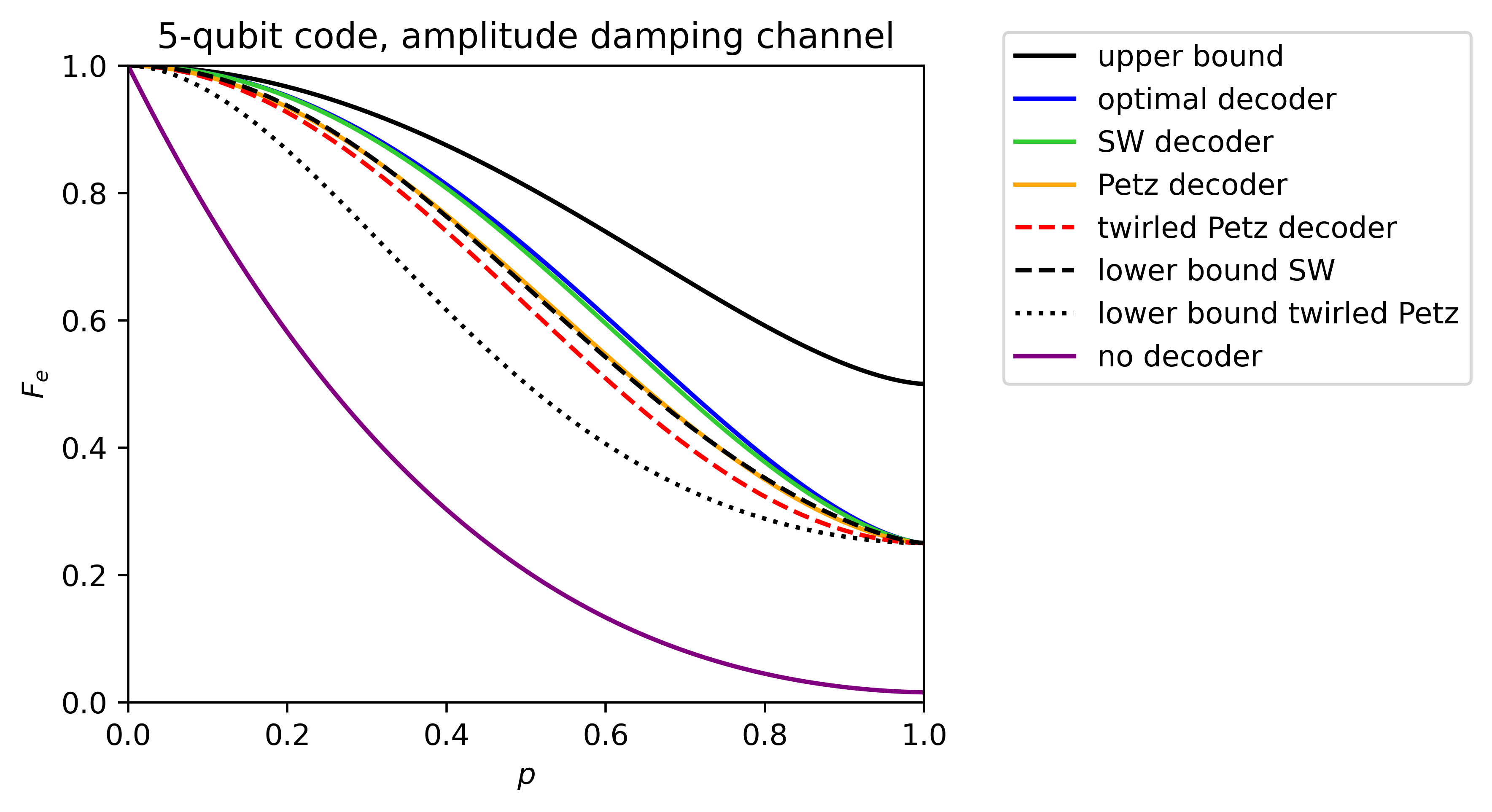
5-qubit code, amplitude damping channel. The noisy channel is given by where is again the amplitude damping channel. The initial state is defined as where is defined as in (devitt2013quantum, , Eq. (54)–(56)) (see also the original work laflamme1996perfect ) and , where denotes the Pauli- gate.
For each of these settings, the performance of the SW, the Petz, and the twirled Petz decoder has been computed as measured by the entanglement fidelity. The results are presented in Figure 2, where is plotted for being the SW decoder (green), the Petz decoder (orange), or the twirled Petz decoder (red, dashed). For illustrative purposes, the following additional curves are plotted in Figure 2: The upper bound (black) is a plot of , which is an upper bound on the entanglement fidelity of an optimal decoder, see Remark 4. The curve labelled as optimal decoder (blue) represents the entanglement fidelity of an optimal decoder, i.e., . This expression has been computed by solving the corresponding semidefinite program (fletcher2007optimum, , Section IV). To solve this semidefinite program for the 5-qubit code, we have taken advantage of the fact that the quantity of interest can be computed via a semidefinite program in a lower-dimensional setting (fletcher2007optimum, , Section V). The lower bound SW (black, dashed) curve is a plot of , which is a lower bound on , see (3.3). The lower bound twirled Petz (black, dotted) curve is a plot of , which is a lower bound on , see (3.15). The no decoder (purple) curve is a plot of where is taken to be the identity channel.
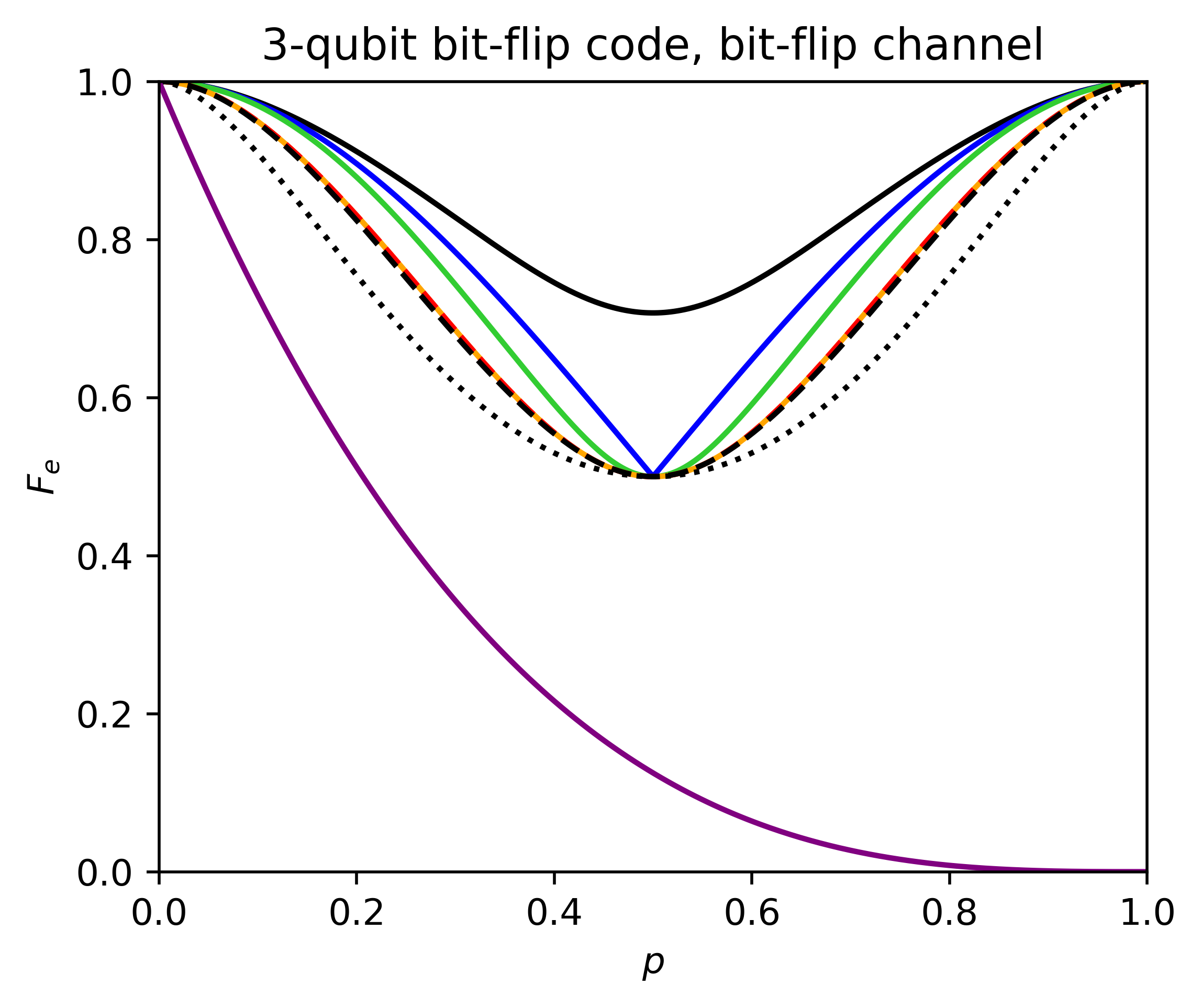
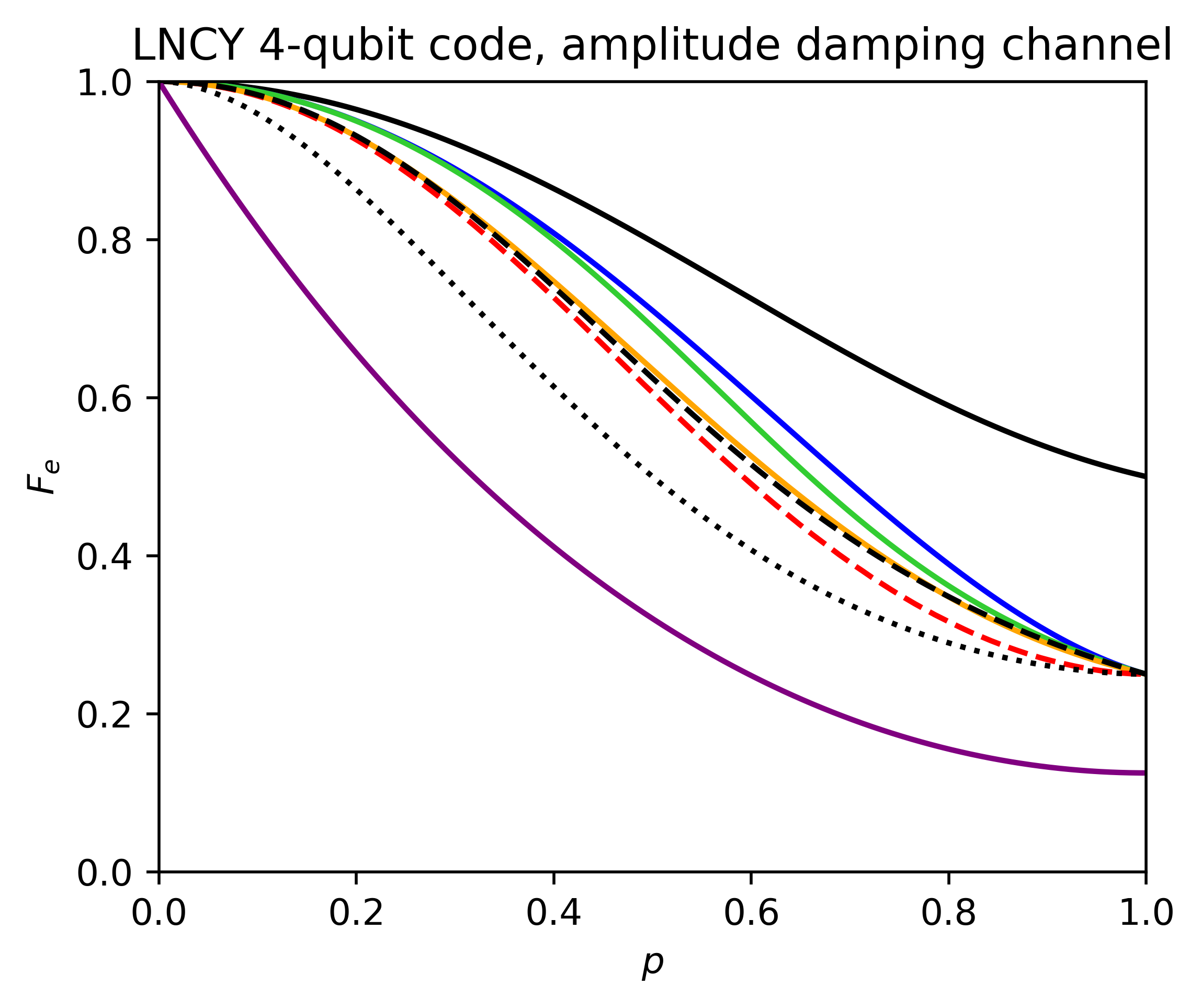
The results presented in Figure 2 imply the following qualitative statements.
-
•
3-qubit bit-flip code, bit-flip channel. The SW decoder performs strictly better than the Petz decoder for any ; for , their performances coincide. The Petz decoder and the twirled Petz decoder have the same entanglement fidelity. In comparison, the lower bound SW is slightly smaller if .
-
•
LNCY 4-qubit code, amplitude damping channel. The SW decoder performs strictly better than the Petz decoder for any ; for , their performances coincide. The entanglement fidelity of the twirled Petz decoder is strictly smaller than that of the Petz decoder for any . The lower bound SW is slightly smaller or greater than the entanglement fidelity of the Petz decoder depending on the value of .
-
•
5-qubit code, amplitude damping channel. The SW decoder performs strictly better than the Petz decoder for any ; for , their performances coincide. The entanglement fidelity of the twirled Petz decoder is strictly smaller than that of the Petz decoder for any . The lower bound SW is slightly smaller or greater than the entanglement fidelity of the Petz decoder depending on the value of .
These conclusions allow us to answer the questions raised above as follows.
- Answer to Question 1
-
In all three settings, the SW decoder performs better than the Petz decoder, and in most cases it performs strictly better.
- Answer to Question 2
-
Depending on the setting and the parameter value , it is possible that is greater or smaller than . Therefore, these two quantities cannot be ordered by the same inequality for all possible .
4 Conclusion
We defined two specific decoders for one-shot entanglement transmission, the Petz decoder and the twirled Petz decoder, and analyzed their performance as measured by the entanglement fidelity. The main results of this analysis were presented in Theorem 4, accompanied by Corollary 5. Theorem 4 asserts that the Petz decoder for one-shot entanglement transmission of over a noisy channel satisfies
| (4.1) |
where and is a purification of . (4.1) is a closed-form expression for the entanglement fidelity of the Petz decoder in terms of . (4.1) can be expressed in an alternative way by duality, as shown in Corollary 5: The entanglement fidelity of the Petz decoder is determined by the singly minimized Petz Rényi mutual information of order associated with a complementary channel as
| (4.2) |
Furthermore, Corollary 5 asserts that the twirled Petz decoder cannot outperform the Petz decoder. Thus, one-shot entanglement transmission is a task where the simpler Petz map suffices for recovery and even performs better. For other settings where the twirled Petz map is unnecessary and the Petz map is sufficient for recovery, see alhambra2017dynamical ; alhambra2018work ; swingle2019recovery ; cotler2019entanglement ; chen2020entanglement .
Our results on the performance of the Petz decoder can be compared with similar results on the performance of the SW decoder (Theorem 1, Corollary 2). For the SW decoder, it is not known whether the entanglement fidelity can be written as a closed-form expression of . However, at least a lower bound on the performance can be proved that is a closed-form expression of : According to Theorem 1, we have
| (4.3) |
which is structurally similar to (4.1). This lower bound can be expressed in an alternative way by duality, as shown in Corollary 2: The entanglement fidelity of the SW decoder is lower-bounded by the non-minimized sandwiched Rényi mutual information of order associated with a complementary channel as
| (4.4) |
which is structurally similar to (4.2).
Our analytical results leave open the question of whether the SW decoder or the Petz decoder performs better. However, the numerical results in Section 3.3 provide a partial answer: For all three settings examined there, the SW decoder outperformed the Petz decoder. At present, we are not aware of any example where the SW decoder performs strictly worse than the Petz decoder. Another question left open by our analytical results is how (4.2) compares to the lower bound on the entanglement fidelity of the SW decoder in (4.4). Our numerical results show that this question does not have a universal answer: For some parameter ranges, (4.2) was greater than the right-hand side of (4.4), while for others the opposite was true. Thus, although the SW decoder typically performs better than the Petz decoder, our analytical estimates of the performance of these decoders – given by the right-hand sides of (4.2) and (4.4) – appear to be comparably good.
The numerical results in Section 3.3 also enable a comparison between the performance of the Petz decoder and that of an optimal decoder. The latter’s performance can be formulated as a semidefinite program fletcher2007optimum , making its numerical computation relatively easy. In contrast, the Petz decoder has the advantage that its analytical form is known a priori, and its performance has a closed-form expression in terms of , as shown in (4.1). These features are typically absent in an optimal decoder, but could be beneficial in certain applications.
Our result in (4.2) provides an operational interpretation of the singly minimized Petz Rényi mutual information of order for states of the form , i.e., states obtained from a bipartite pure state by acting on one of its parts with a CPTP map. For such states, (4.2) shows that quantifies how well the initial state is recovered by the Petz decoder from a system that is the output of a channel complementary to . Thus, (4.2) reveals a connection between information recovery via the Petz map (left-hand side) and a corresponding information measure (right-hand side).
Recently, the Petz map and the twirled Petz map have attracted interest in the research field of quantum theories of spacetime, as they provide a tool for entanglement wedge reconstruction vardhan2023petzrecoverysubsystemsconformal ; bahiru2023explicit ; cotler2019entanglement ; chen2020entanglement . In this context, it has been conjectured that there exists a deeper connection between information recovery via the Petz map and the reflected entropy penington2020replicawormholesblackhole ; akers2022page . Our result in (4.2) suggests that a modified version of this conjecture holds. As we will show in future work burri2024minreflected , the singly minimized Petz Rényi mutual information of order naturally serves as an upper bound for the min-reflected entropy. Consequently, by (4.2), it can be inferred that the min-reflected entropy provides an upper bound for the entanglement fidelity of the Petz decoder. This establishes a general relationship between information recovery via the Petz map and the min-reflected entropy. It would be interesting to explore how tight this relationship is. More broadly, it remains an open question for future research whether there are even deeper connections between information recovery (via the Petz map) and the (min-)reflected entropy.
Acknowledgements.
I am grateful to Renato Renner for discussions and valuable comments on a draft of this work, and to Christophe Piveteau and Lukas Schmitt for discussions. This work was supported by the Swiss National Science Foundation via project No. 20QU-1_225171 and the National Centre of Competence in Research SwissMAP, and the Quantum Center at ETH Zurich.Appendix A Construction of Schumacher-Westmoreland decoder
In this section, we summarize the construction of the SW decoder schumacher2001approximate . While our summary qualitatively follows the original description in schumacher2001approximate , it differs from the original presentation in a few places to make the construction more explicit and specific. For instance, we have chosen to fix the dimensions of certain auxiliary systems for technical convenience, whereas the original work schumacher2001approximate leaves them unspecified. (Specifically, the dimension of will be the rank of , and the dimension of will be .)
Let . Let be the rank of , and let be a -dimensional Hilbert space. Let be such that . Consider a Schmidt decomposition of : Let be a probability distribution, and let be orthonormal bases for such that
| (A.1) |
Let be isomorphic to , let , and let be an isometry such that for all . Let . Consider a spectral decomposition of : Let be a probability distribution and let be an orthonormal basis for such that
| (A.2) |
Let be isomorphic to , let (which is isomorphic to ), and let us define the following objects.
| (A.3) | ||||
| (A.4) | ||||
| (A.5) | ||||
| (A.6) | ||||
| (A.7) |
Consider a singular value decomposition of : Let be unitary and such that for a suitable positive semidefinite operator that is diagonal in the orthonormal basis . Let .
Let be an arbitrary but fixed unit vector. Then,
| (A.8) |
where the last equality follows from (A.5). Therefore, there exists a unitary such that
| (A.9) |
Let us define the following objects.
| (A.10) | ||||
| (A.11) | ||||
| (A.12) |
The SW decoder for is then defined as
| (A.13) |
Appendix B Proofs and remarks
B.1 Proof of Theorem 1
Proof.
Case 1: . Then, has the same form as in the construction of the SW decoder. Consequently, all objects can be defined as in the construction of the SW decoder, see Section A. In addition, we define the following unit vectors.
| (B.1) | ||||
| (B.2) |
The second equality in (B.1) follows from (A.1), (A.2), and (A.3) because . We have
| (B.3) | |||
| (B.4) | |||
| (B.5) | |||
| (B.6) |
(B.4) follows from (A.11), (A.12), and (B.2). (B.5) follows from (A.7) and (B.1). (B.6) follows from (A.1) and (A.2).
We are now ready to analyze the quantity of interest.
| (B.7) | ||||
| (B.8) | ||||
| (B.9) | ||||
| (B.10) | ||||
| (B.11) | ||||
| (B.12) | ||||
| (B.13) | ||||
| (B.14) | ||||
| (B.15) | ||||
| (B.16) | ||||
| (B.17) |
(B.8) holds because . (B.9) follows from the monotonicity of the fidelity under CPTP maps (and thus, under the partial trace over ). (B.10) follows from (A.13) and (B.6). (B.11) follows from the monotonicity of the fidelity under CPTP maps (and thus, under ). (B.12) follows from (A.10). (B.14) follows from (A.9) and (B.2). (B.15) follows from (A.5) and (B.1). (B.16) follows from (A.6). (B.17) follows from (A.3).
By taking the logarithm, we can conclude that
| (B.18) | ||||
| (B.19) | ||||
| (B.20) |
(B.20) holds by a duality relation for the non-minimized sandwiched Rényi mutual information (or, equivalently, for the minimized generalized Petz Rényi mutual information) hayashi2016correlation ; burri2024doublyminimizedpetzrenyi ; burri2024doublyminimizedsandwichedrenyi .
Case 2: . Let be a Hilbert space whose dimension is . Let be such that . Since both and are purifications of , there exists an isometry such that . Let . Then,
| (B.21) |
We can conclude that
| (B.22) |
The inequality in (B.22) follows from case 1. The first equality in (B.22) follows from the invariance under local isometries of the minimized generalized Petz Rényi mutual information burri2024doublyminimizedpetzrenyi , and the second equality follows from (B.21). ∎
B.2 Proof of Corollary 2
Proof of (3.4).
(3.4) follows from Theorem 1 and the duality of the non-minimized sandwiched Rényi mutual information hayashi2016correlation ; burri2024doublyminimizedpetzrenyi ; burri2024doublyminimizedsandwichedrenyi . ∎
Proof of (3.5).
Since is a complementary channel to , there exists an isometry such that and for all . Let . Then
| (B.23) | ||||
| (B.24) |
We can conclude that
| (B.25) | ||||
| (B.26) | ||||
| (B.27) |
(B.25) follows from (3.4). (B.26) follows from (B.23) and the duality of the non-minimized sandwiched Rényi mutual information hayashi2016correlation ; burri2024doublyminimizedpetzrenyi ; burri2024doublyminimizedsandwichedrenyi . (B.27) follows from (B.24). ∎
Proof of (3.7).
Let be such that .
| (B.28) | ||||
| (B.29) | ||||
| (B.30) | ||||
| (B.31) | ||||
| (B.32) | ||||
| (B.33) |
(B.28) follows from (3.4). (B.29) follows from the monotonicity of the sandwiched divergence in the Rényi order mueller2013quantum . (B.31) follows from the duality of the conditional entropy tomamichel2014relating . (B.32) follows from (B.31) because . (B.33) follows from (B.31) because is a pure state and . ∎
B.3 More details on Remark 2
Based on the construction of the SW decoder (see Appendix A), the original work on the SW decoder schumacher2001approximate contains a proof of the following inequalities.
| (B.34) | ||||
| (B.35) | ||||
| (B.36) | ||||
| (B.37) | ||||
| (B.38) |
(B.34) follows from similar arguments as in (B.7)–(B.17). (B.35) follows from the Fuchs-van de Graaf inequality fuchs2004cryptographic . (B.36) follows from the quantum Pinsker inequality hiai1981sufficiency . (B.37) follows from (B.31), (B.32), and the definition of in (3.6). The original proof therefore relies on a duality relation in (B.37), namely, the duality of the conditional entropy, see (B.31). In contrast, our proof employs a different duality relation at an earlier stage of the proof, namely, the duality of the non-minimized sandwiched Rényi mutual information, see (B.20).
B.4 Proof of Theorem 4
Proof of (3.8).
B.5 Proof of Corollary 5
In order to prove Corollary 5, we will use the following lemma.
Lemma 7.
Let be positive semidefinite. Then, for all
| (B.51) |
Proof.
The first inequality in (B.51) follows from the assumption that and are positive semidefinite. It remains to prove the second inequality in (B.51). Consider a spectral decomposition of : Let be an orthonormal basis for such that where are the eigenvalues of . Then
| (B.52) | ||||
| (B.53) | ||||
| (B.54) | ||||
| (B.55) |
(B.53) holds because is positive semidefinite, which entails that is self-adjoint (). ∎
We will now prove Corollary 5.
Proof of (a).
(3.11) follows from (3.9) in Theorem 4 because by duality hayashi2016correlation ; burri2024doublyminimizedpetzrenyi ; burri2024doublyminimizedsandwichedrenyi . (3.12) follows from (3.11) by the same argument as in the proof of (3.5), see Appendix B.2. ∎
Proof of (b).
B.6 Proof of Corollary 6
We will prove the equivalence of the statements by proving certain implications.
(a) (f).
Suppose (a) holds, i.e., there exists such that . Then, , so
| (B.65) |
Let be such that . Then,
| (B.66) | ||||
| (B.67) | ||||
| (B.68) |
(B.66) follows from the duality of the conditional entropy. (B.67) holds because is a pure state. The equality in (B.68) follows from (B.65). The inequality in (B.68) follows from the data processing inequality for the conditional entropy. We can conclude that , which implies that . ∎
(f) (e).
Let be such that . Suppose (f) holds, i.e., . Then,
| (B.69) | ||||
| (B.70) |
The first equality in (B.69) follows from the duality of the conditional entropy, and the second equality follows from . The first equality in (B.70) follows from , and the second equality follows from the fact that is a pure state. ∎
(e) (b) (c) (d).
(b) (c) (d) (a).
This implication is trivial because from (a) can be chosen to be or , respectively. ∎
References
- (1) Benjamin Schumacher. Sending entanglement through noisy quantum channels. Physical Review A, 54:2614–2628, 1996. DOI: 10.1103/PhysRevA.54.2614.
- (2) Benjamin Schumacher and Michael A. Nielsen. Quantum data processing and error correction. Physical Review A, 54(4):2629–2635, 1996. DOI: 10.1103/PhysRevA.54.2629.
- (3) Benjamin Schumacher and Michael D. Westmoreland. Approximate quantum error correction, 2001. DOI: 10.48550/arXiv.quant-ph/0112106.
- (4) Andrew S. Fletcher, Peter W. Shor, and Moe Z. Win. Optimum quantum error recovery using semidefinite programming. Physical Review A, 75:012338, 2007. DOI: 10.1103/PhysRevA.75.012338.
- (5) Michael Reimpell and Reinhard F. Werner. Iterative optimization of quantum error correcting codes. Physical Review Letters, 94(8), 2005. DOI: 10.1103/PhysRevLett.94.080501.
- (6) Michael Reimpell, Reinhard F. Werner, and Koenraad Audenaert. Comment on “Optimum Quantum Error Recovery using Semidefinite Programming”, 2006. DOI: 10.48550/arXiv.quant-ph/0606059.
- (7) Nilanjana Datta and Min-Hsiu Hsieh. One-shot entanglement-assisted quantum and classical communication. IEEE Transactions on Information Theory, 59(3):1929–1939, 2013. DOI: 10.1109/TIT.2012.2228737.
- (8) Salman Beigi, Nilanjana Datta, and Felix Leditzky. Decoding quantum information via the Petz recovery map. Journal of Mathematical Physics, 57(8):082203, 2016. DOI: 10.1063/1.4961515.
- (9) Dénes Petz. Sufficient subalgebras and the relative entropy of states of a von Neumann algebra. Communications in Mathematical Physics, 105(1):123–131, 1986. DOI: 10.1007/BF01212345.
- (10) Dénes Petz. Sufficiency of channels over von Neumann algebras. The Quarterly Journal of Mathematics, 39(1):97–108, 1988. DOI: 10.1093/qmath/39.1.97.
- (11) Masanori Ohya and Dénes Petz. Quantum Entropy and Its Use. Springer, Berlin, 1993.
- (12) Dénes Petz. Monotonicity of quantum relative entropy revisited. Reviews in Mathematical Physics, 15(01):79–91, 2003. DOI: 10.1142/S0129055X03001576.
- (13) Marius Junge, Renato Renner, David Sutter, Mark M. Wilde, and Andreas Winter. Universal recovery maps and approximate sufficiency of quantum relative entropy. Annales Henri Poincaré, 19(10):2955–2978, 2018. DOI: 10.1007/s00023-018-0716-0.
- (14) Debbie W. Leung, Michael A. Nielsen, Isaac L. Chuang, and Yoshihisa Yamamoto. Approximate quantum error correction can lead to better codes. Physical Review A, 56(4):2567–2573, 1997. DOI: 10.1103/PhysRevA.56.2567.
- (15) Raymond Laflamme, Cesar Miquel, Juan Pablo Paz, and Wojciech Hubert Zurek. Perfect quantum error correcting code. Physical Review Letters, 77:198–201, 1996. DOI: 10.1103/PhysRevLett.77.198.
- (16) Dénes Petz. Quasi-entropies for finite quantum systems. Reports on Mathematical Physics, 23(1):57–65, 1986. DOI: 10.1016/0034-4877(86)90067-4.
- (17) Simon M. Lin and Marco Tomamichel. Investigating properties of a family of quantum Rényi divergences. Quantum Information Processing, 14(4):1501–1512, 2015. DOI: 10.1007/s11128-015-0935-y.
- (18) Marco Tomamichel. Quantum Information Processing with Finite Resources. Springer, 2016. DOI: 10.1007/978-3-319-21891-5.
- (19) Martin Müller-Lennert, Frédéric Dupuis, Oleg Szehr, Serge Fehr, and Marco Tomamichel. On quantum Rényi entropies: A new generalization and some properties. Journal of Mathematical Physics, 54(12):122203, 2013. DOI: 10.1063/1.4838856.
- (20) Mark M. Wilde, Andreas Winter, and Dong Yang. Strong Converse for the Classical Capacity of Entanglement-Breaking and Hadamard Channels via a Sandwiched Rényi Relative Entropy. Communications in Mathematical Physics, 331:593–622, 2014. DOI: 10.1007/s00220-014-2122-x.
- (21) Masahito Hayashi and Marco Tomamichel. Correlation detection and an operational interpretation of the Rényi mutual information. Journal of Mathematical Physics, 57(102201), 2016. DOI: 10.1063/1.4964755.
- (22) Laura Burri. Doubly minimized Petz Rényi mutual information: Properties and operational interpretation from direct exponent, 2024. DOI: 10.48550/arXiv.2406.01699.
- (23) Manish K. Gupta and Mark M. Wilde. Multiplicativity of Completely Bounded -Norms Implies a Strong Converse for Entanglement-Assisted Capacity. Communications in Mathematical Physics, 334(2):867–887, 2014. DOI: 10.1007/s00220-014-2212-9.
- (24) Laura Burri. Doubly minimized sandwiched Rényi mutual information: Properties and operational interpretation from strong converse exponent, 2024. DOI: 10.48550/arXiv.2406.03213.
- (25) Göran Lindblad. Completely positive maps and entropy inequalities. Communications in Mathematical Physics, 40:147–151, 1975. DOI: 10.1007/BF01609396.
- (26) Armin Uhlmann. Relative Entropy and the Wigner-Yanase-Dyson-Lieb Concavity in an Interpolation Theory. Communications in Mathematical Physics, 54:21, 1977. DOI: 10.1007/BF01609834.
- (27) Mark M. Wilde. Recoverability in quantum information theory. Proceedings of the Royal Society A: Mathematical, Physical and Engineering Sciences, 471(2182):20150338, 2015. DOI: 10.1098/RSPA.2015.0338.
- (28) David Sutter, Marco Tomamichel, and Aram W. Harrow. Strengthened Monotonicity of Relative Entropy via Pinched Petz Recovery Map. IEEE Transactions on Information Theory, 62(5):2907–2913, 2016. DOI: 10.1109/TIT.2016.2545680.
- (29) Howard Barnum and Emanuel Knill. Reversing quantum dynamics with near-optimal quantum and classical fidelity. Journal of Mathematical Physics, 43(5):2097–2106, 2002. DOI: 10.1063/1.1459754.
- (30) Hui Khoon Ng and Prabha Mandayam. Simple approach to approximate quantum error correction based on the transpose channel. Physical Review A, 81(6), 2010. DOI: 10.1103/PhysRevA.81.062342.
- (31) Bikun Li, Zhaoyou Wang, Guo Zheng, and Liang Jiang. Optimality Condition for the Transpose Channel, 2024. DOI: 10.48550/arXiv.2410.23622.
- (32) Simon J. Devitt, William J. Munro, and Kae Nemoto. Quantum error correction for beginners. Reports on Progress in Physics, 76(7):076001, 2013. DOI: 10.1088/0034-4885/76/7/076001.
- (33) Álvaro M. Alhambra and Mischa P. Woods. Dynamical maps, quantum detailed balance, and the Petz recovery map. Physical Review A, 96(2), 2017. DOI: 10.1103/PhysRevA.96.022118.
- (34) Álvaro M. Alhambra, Stephanie Wehner, Mark M. Wilde, and Mischa P. Woods. Work and reversibility in quantum thermodynamics. Physical Review A, 97(6), 2018. DOI: 10.1103/PhysRevA.97.062114.
- (35) Brian G. Swingle and Yixu Wang. Recovery map for fermionic Gaussian channels. Journal of Mathematical Physics, 60(7), 2019. DOI: 10.1063/1.5093326.
- (36) Jordan Cotler, Patrick Hayden, Geoffrey Penington, Grant Salton, Brian Swingle, and Michael Walter. Entanglement Wedge Reconstruction via Universal Recovery Channels. Physical Review X, 9:031011, 2019. DOI: 10.1103/PhysRevX.9.031011.
- (37) Chi-Fang Chen, Geoffrey Penington, and Grant Salton. Entanglement Wedge Reconstruction using the Petz map. Journal of High Energy Physics, 2020(1), 2020. DOI: 10.1007/JHEP01(2020)168.
- (38) Shreya Vardhan, Annie Y. Wei, and Yijian Zou. Petz recovery from subsystems in conformal field theory, 2023. DOI: 10.48550/arXiv.2307.14434.
- (39) Eyoab Bahiru and Niloofar Vardian. Explicit reconstruction of the entanglement wedge via the Petz map. Journal of High Energy Physics, 2023(7), 2023. DOI: 10.1007/JHEP07(2023)025.
- (40) Geoff Penington, Stephen H. Shenker, Douglas Stanford, and Zhenbin Yang. Replica wormholes and the black hole interior. Journal of High Energy Physics, (3), 2022. DOI: 10.1007/JHEP03(2022)205.
- (41) Chris Akers, Thomas Faulkner, Simon Lin, and Pratik Rath. The Page curve for reflected entropy. Journal of High Energy Physics, 2022(6), 2022. DOI: 10.1007/JHEP06(2022)089.
- (42) Laura Burri. Min-reflected entropy (to appear), 2024.
- (43) Marco Tomamichel, Mario Berta, and Masahito Hayashi. Relating different quantum generalizations of the conditional Rényi entropy. Journal of Mathematical Physics, 55(8), 2014. DOI: 10.1063/1.4892761.
- (44) Christopher A. Fuchs and Jeroen van de Graaf. Cryptographic Distinguishability Measures for Quantum Mechanical States, 1997. DOI: 10.48550/arXiv.quant-ph/9712042.
- (45) Fumio Hiai, Masanori Ohya, and Makoto Tsukada. Sufficiency, KMS condition and relative entropy in von Neumann algebras. Pacific Journal of Mathematics, 96:99–109, 1981. DOI: 10.2140/PJM.1981.96.99.