Data efficiency and long-term prediction capabilities for neural operator surrogate models of edge plasma simulations

Abstract

Simulation-based plasma scenario development plays a crucial role in designing next-generation tokamaks and fusion power plants. However, the inclusion of high-fidelity simulations of Scrape-Off Layer (SOL) turbulence and transient MHD events such as Edge Localized Modes (ELMs) in highly iterative applications remains computationally prohibitive, limiting their use in iterative design and control workflows. Understanding these phenomena is vital, as they govern heat flux on plasma-facing components, influencing reactor performance and material lifetime. This study explored Fourier Neural Operators (FNOs) as surrogate models to accelerate plasma simulations from the JOREK MHD and STORM turbulence codes.

FNOs were trained on single-step rollouts and evaluated in terms of long-term predictive accuracy in an auto-regressive manner. To mitigate the computational burden of dataset generation, a transfer learning strategy was explored, leveraging low-fidelity simulations to improve performance on high-fidelity datasets. These results showed that FNOs effectively captured initial plasma evolution, including blob movement and density source localization for JOREK and STORM, respectively. However, long rollouts accumulated errors and exhibited sensitivity to certain physical phenomena, leading to non-monotonic error spikes. Transfer learning significantly reduced errors for small dataset sizes and short rollouts, achieving an order-of-magnitude reduction when transfering from low- to high-fidelity datasets. However, its effectiveness diminished with longer rollouts and larger dataset sizes, especially when applied to datasets with significantly different dynamics. Attempts to transfer models to previously unseen variables in simulations were unsuccessful, underscoring the limitations of transfer learning in this context.

These findings demonstrate the promise of neural operators for accelerating fusion-relevant PDE simulations. However, they also highlight key challenges: improving long-term accuracy to mitigate error accumulation, capturing critical physical behaviors, and developing robust surrogates that effectively leverage multi-fidelity, multi-physics datasets.

• December 2024

1 Introduction

1.1 Motivation

Modelling of the edge plasma is fundamental to ensure appropriate divertor and core performance, and their reliable characterisation is desirable for not just designing and interpreting the current generation of experiments, but to inform the next generation devices like ITER and STEP [1, 2]. However, modelling plasma is computationally intensive, requiring the solution of strongly coupled partial differential equations (PDEs), which are often analytically intractable. Numerical approximation schemes provide a practical approach, balancing accuracy and computational efficiency, as implemented in frameworks such as BOUT++ [3], JOREK [4], JINTRAC [5], and SOLPS [6].

However, even for reduced-order models, which are often 1 dimensional (e.g., DIV1D [7]), the computational cost is still high or even prohibitive for iterative applications, such as optimisation, or real-time control. The MHD code JOREK, which simulates transient MHD events such as Edge Localized Modes (ELMs), is a prominent example of this issue. While ELM simulations are crucial for designing tokamaks and their control systems [8], accurately simulating ELM behavior in DEMO-class devices is slow and takes up large computational resources.

Beyond transient MHD events, turbulence in the Scrape-Off Lyaer (SOL) drives fine-scale, continuous heat transport by pushing particles across field lines. The SOL is known to be dominated by coherent structures known as filaments, which play a crucial role in transporting plasma particles over large distances from the separatrix. These filaments contribute to shaping the time-averaged density profile in the SOL and simulating them poses a major computational challenge [9]. The contrast in time scales between parallel and perpendicular transport imposes strict time-step limitations, making it difficult to balance accuracy and efficiency. Consequently, current solvers cannot yet routinely simulate turbulence at the scale of DEMO-class reactors, focusing instead on smaller experimental devices like TCV or ASDEX Upgrade [10].

Additionally, numerical solvers often have to be specifically tailored to the equations and spatial geometry they address [11], are challenging to deploy quickly due to their complex software infrastructure and library dependencies, and these solvers may fail to converge when integrated into larger simulation frameworks, often due to model mismatches or the need for expert manual intervention.

Neural network (NN) based surrogate models offer a promising avenue to enable the fast, inexpensive estimation of plasma states given the initial and boundary conditions for a physical model of choice. For example, Convolutional Neural Networks (CNNs) have been applied to emulate the behaviour of SOLPS [6, 12, 13] over a restricted area of its parameter space, demonstrating orders of magnitude speedup. Nevertheless, solutions derived from CNNs lack discretization invariance (both spatially and temporally), and therefore are applicable only to the specific discretization of the numerical PDE solution that they were trained on. Recent work has introduced Neural Operators (NOs) [14], a family of surrogate models that learn infinite-dimensional mappings between function spaces, and are thus capable of learning a continuous, discretization-invariant representation of PDE solutions [15, 16]. The Fourier Neural Operator (FNO), where convolutional filters are learned in Fourier space, has proved a particularly successful architecture for modelling PDEs with NNs [15].

1.2 Similar works

Machine learning-based surrogate models, including neural operators (NOs), are being applied in plasma physics to provide rapid approximations for various problems. In fusion applications, these include emulating turbulent transport [17, 18], estimating the Tritium breeding ratio [19], and modelling edge plasma behavior [20, 13].

Recent approaches to neural PDE surrogates can be split into thee main groups [21]: (1) approaches that directly learn to approximate the PDE [22] (2) data driven approaches that map the current state of a system to its future state using a learned evolution operator [23, 24] and (3) hybrid approaches that combine neural networks with traditional numerical solvers [25, 26]. For time-dependent PDEs, many approaches rely on autoregressive rollouts, where outputs from prior steps were fed back as inputs to compute solutions over long time horizons. Since directly predicting long-term evolution is highly challenging, autoregressive modeling allows the system to approximate future states incrementally. However, a key drawback of autoregressive rollouts is the accumulation of errors at each prediction step, which can cause the predicted trajectories to diverge from the ground truth over time [21, 24, 27]. Traditional numerical methods mitigate such instabilities using implicit schemes or explicit methods such as adaptive step sizes to improve accuracy and stability [11, 28]. In contrast, neural operators deployed autoregressively operate in a Markovian fashion, lacking a forcing function to correct errors. Consequently, evaluating their performance over longer time horizons is crucial for assessing their reliability in fusion applications.

Despite these advances, the application of NOs to fusion-related time-dependent problems remains limited as the use of machine learning, particularly neural operators, in fusion research is still a relatively new and emerging area. A first exploration of FNOs for emulation of MHD was presented in [20], where it was shown that the FNO outperforms non discretization-invariant, CNN-based architectures. In the same study, the FNO was shown to be capable of accurately predicting the short-term evolution of plasma in the Mega Ampere Spherical Tokamak visible camera images. In another study, [29] benchmarked a range of NOs for reproducing DIV1D simulations, with FNOs serving as a competitive baseline.

Building on these advances, previous work by the authors introduced the Neural-Parareal framework [25], which focuses on integrating NOs as coarse solvers within the Parareal method - a time-parallelization technique for High-Performance Computing (HPC) simulations. This approach focused on dynamically training NOs using data generated by the framework to improve surrogate model accuracy and speed-up. In contrast, this work examines the performance of NOs over longer time periods independently, with a particular focus on their use in transfer learning to enhance data efficiency.

Additionally, creating simulation data to train surrogate models is often prohibitively expensive, requiring computationally-expensive iterative solvers such as finite-volume schemes and finite-element methods to be run on supercomputers. Strategies that focus surrogate model training (and thus generation of simulation data) on the most informative regions of parameter space have been proposed in [30, 31, 32], showing significant data efficiency gains. In contrast, this work focuses on transfer learning, which leverages other informative datasets - such as lower-fidelity simulations that are more readily available - to improve the performance of surrogate models, offering a different approach to enhancing data efficiency. Following the success of transfer learning in computer vision and natural language processing tasks [33, 34, 35, 36, 37], transfer learning has emerged as a promising technique for data-efficient learning in the machine learning community. A common approach used is fine-tuning which involves reusing a model developed for one task as the starting point for another, related task [36]. By leveraging knowledge acquired from a source domain, transfer learning can improve learning efficiency and performance in target domains, offering a practical solution for domains where high-fidelity data is scarce or expensive to generate. Prior work has explored transfer learning in neural operator surrogates, demonstrating its potential for data efficiency improvements in simulation-based tasks [38]. However, the applicability and scalability of this technique across distinct simulation frameworks and fidelity levels remains an open question, as does its capability to handle long-term trajectory predictions.

1.3 Overview of this work

This work presents Fourier Neural Operator (FNO)-based surrogate models, implemented using the PDEArena library [39], for two widely used plasma simulation codes: STORM [40] and JOREK [4]. STORM, built on the BOUT++ framework, is a fluid code focused on modelling turbulence and transport processes in the SOL region. JOREK, on the other hand, is a widely adopted code for studying large-scale MHD instabilities in both core and edge regions of tokamaks [41]. This paper focuses on the FNO due to its demonstrated efficiency on medium-scale PDE problems like the datasets utilized in the present work [42, 43].

The investigation focused on the following objectives:

• Understanding long-term prediction accuracy in neural operator surrogate models. Errors in autoregressive rollouts compound over time, leading to instabilities. This study also examined how trajectory-specific dynamics contribute to error accumulation. Particular attention was given to transitions or significant events within the trajectory, as these could exacerbate error growth.

• Exploring the potential of transfer learning in neural operators. This study investigated transfer learning as a strategy to enhance data efficiency by leveraging knowledge from related datasets. Models trained from scratch were compared with those fine-tuned using transfer learning, and their performance was evaluated in terms of how it scaled with dataset size and rollout length. The objective was to assess the feasibility of using transfer learning across diverse scenarios relevant to fusion modelling, providing insights into its strengths and limitations. Specifically three scenarios were explored:

  1. Cross-Simulation-Code Transfer (between STORM and JOREK): Transfer learning was tested between two independently developed simulation codes with distinct applications and physics models. This scenario evaluated the adaptability of neural operator surrogates to handle entirely different simulation frameworks.

  2. Cross-Fidelity Transfer (within JOREK): The transfer of knowledge was explored between two datasets of differing fidelity levels, specifically from low-fidelity to high-fidelity JOREK simulations. This approach evaluated the potential of transfer learning to reduce the computational burden of high-fidelity modelling by using low-cost, lower-fidelity simulations as a foundation.

  3. Cross-Variable Transfer (within JOREK): A key challenge encountered when transferring from low- to high-fidelity simulations was that the target dataset contained variables absent in the source dataset. Many deep learning architectures such as FNO lack the flexibility to seamlessly incorporate prior knowledge from learned variables into datasets with new variables. To address this, experiments with a two-step transfer learning approach were carried out: first, transferring knowledge from the low-fidelity dataset to the common variables in the high-fidelity dataset, followed by a second transfer step to extend the learned representations to the variables unique to the target dataset.

2 Problem Setting

2.1 Dataset

In this work, training datasets created from STORM [40] and JOREK [4] simulations were used which have already been adopted in several studies [25, 44, 45]. JOREK is designed to simulate large-scale MHD-instabilities in the core and edge plasma region, whereas STORM is a fluid code focused on modelling turbulance and transport processes in the SOL at much smaller scales. All simulations in these datasets were run in simplified 2D rectangular slab geometry (with toroidal curvature). The long term goal will be to expand to 3D cases with more complex simulations in full toroidal geometry, which is left for future work. Dimensions of the dataset are be found in table 1.

Dataset name	Dataset size	Trajectory length (num timesteps)	Num variables	Dimensions
STORM	1000 trajectories	1000 per traj	2	384x256
Electrostatic JOREK	2000 trajectories	200 per traj	2	100x100
Reduced-MHD JOREK	11391 slices and 20 trajs	10 per slice and 200 per traj	4	100x100

Table 1: Table describing each dataset’s size, variables and spatial dimensions.

2.1.1 JOREK

is a continuously developed simulation code that is widely used to study large-scale MHD instabilities from the core and edge plasma regions [41]. The JOREK dataset specifically focuses on simulating filamentary blobs in the edge region of a tokamak. Throughout the simulation, the toroidal curvature combined with the pressure gradient of the blobs generates an electric field, resulting in the blobs moving radially outwards (away from the centre of the tokamak). These blobs are expelled out of the hot confined plasma region through turbulence or MHD instabilities, such as Edge-Localised-Modes (ELMs) [4]. These are important to study as ELMs can eject hot plasma filaments onto the machine’s first wall and damage it. The initial conditions of the blobs were generated from uniform distributions in positions (R,Z), amplitudes of density and temperature. The number of blobs were left to vary between 1 and 10 uniformly. Two datasets were generated from JOREK:

1. Electrostatic JOREK simulations evolve three physical variables: density $\rho$, electric potential $\Phi$ and temperature $T$. One auxiliary variable, the toroidal vorticity $\omega$ was used for numerical stability. This model is equivalent to reduced-MHD JOREK dataset below but without the magnetic potential and current components in the model. This dataset is described in further detail in [25].

2. Reduced MHD JOREK as implemented in routine JOREK studies, including a magnetic field but not the parallel velocity. These simulations evolve the four physical variables: $\rho$, $\Phi$, $T$ and poloidal magnetic flux $\Psi$. Two additional auxillary variables $\omega$ and toroidal plasma current density $zj$ were also used. These settings correspond to a higher fidelity compared to the electrostatic case, and required 2.25X more time to generate with similar hardware resources. This dataset was generated in batches for the application [25]. The first batch of data was generated normally resulting in full trajectories (similar to electrostatic JOREK), whereas the three subsequent batches were generated as part of parareal (parallel-in-time) scheme resulting in chunked trajectories. As a consequence of the generation method, the beginning and end of each trajectory chunk does not line up exactly with each other, resulting in 20 individual sets of 10 timesteps referred to as timeslices.

Both JOREK dataset trajectories are evolved for 2000 timesteps (corresponding to a trajectory length of 2000) of approximately 0.15µs each on a high-order Bezier finite-element grid with uniform resolution of 200 by 200 elements. The poloidal 2D slab is centred at a toroidal major radius of 10m with a height and width of 1m. The boundary conditions around the domain are Dirichlet for all variables. High spatial and temporal resolution was chosen to ensure numerical stability during the simulations. An example of the simulations can be seen in figure 1. Additional information about generating the dataset can be found at [25]

2.1.2 STORM

is a fluid code built on the BOUT++ framework which is focused on modelling turbulance and transport processes in the SOL. It has been used to conduct nonlinear flux-driven simulations in double-null tokamak geometry under realistic parameters [3]. The physics model in the STORM simulations used here evolves two variables: the density $\rho$ and electric potential $\Phi$, with a constant background temperature level. A vertical band of density source at a fixed location and amplitude generates fluid turbulence in the radial direction due to the toroidal geometry. The dataset is obtained by varying the amplitude and width of the source which is fixed throughout the timesteps, resulting in the density increasing linearly with time. The simulations were all run in 2D regular slab geometry (384x256) with the dimensions being 150 and 100mm, located around the separatrix, allowing for analysis of much smaller scale turbulence. For STORM, a total of 1000 timesteps were run which evolve density and electric potential.

The neural operator (NO) training focused only on the saturated turbulence phase in STORM when the root-mean-square (RMS) vorticity reached a statistically steady state and fluctuated around a constant value. For practical purposes, this was simplified by including only trajectory timesteps after $t=200$. This approach ensured that the dataset contained trajectories of consistent length and provided a buffer to account for any outliers. This was done as early experiments showed that the transition between the two regimes was extremely difficult to capture accurately due to the highly chaotic nature of turbulence onset. Unlike blobs in the JOREK datasets, which have a clear initial condition, the model found it extremely difficult to predict where the turbulence will start in the STORM cases, as it originated from the growth of very small numerical differences in the background noise. An example of the simulations can be seen in figure 5.

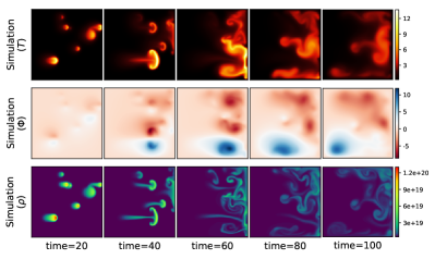
(a) Elecrostatic JOREK

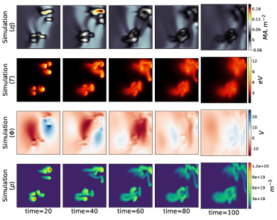
(b) Reduced-MHD JOREK

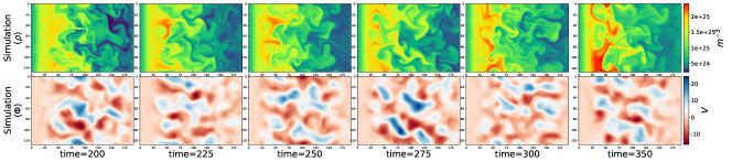
(c) STORM

Figure 1: Example rollout for each of the 3 datasets: (a) electrostatic JOREK dataset, (b) reduced-MHD JOREK dataset and (c) STORM dataset.

2.2 Dataset pre-processing

Given the high-resolution nature of the initial simulations, which were conservatively designed to ensure numerical stability, each dataset was spatially and temporally down-sampled. For example, the spatial resolution of the STORM dataset was reduced from $384\times 256$ to $192\times 128$, while the JOREK datasets (Electrostatic and Reduced MHD) were down-sampled from $200\times 200$ to $100\times 100$. Additionally, the temporal resolution of the JOREK datasets were reduced by a factor of 10, decreasing from 2000 timesteps to 200 by taking every tenth timestep. The dataset resolution that the model is trained on can be increased by reducing the downsampling, but this will result in longer training times and larger model sizes due to the increased data volume. For the current settings, training times are approximately 32, 72, and 144 hours on a single NVIDIA A100 GPU for the reduced-MHD JOREK, electrostatic JOREK, and STORM datasets, respectively, with the resulting model file size being 1.6 GB (after tracing with TorchScript). It is important to note that these specific down-sampling choices are arbitrary; a more extensive study would be required to determine the optimal down-sampling strategy.

The datasets were partitioned into training and testing sets. From the two datasets containing only full trajectories, a roughly 90%/10% split into training/testing was performed; resulting in a dataset split of 799/100 trajectories for STORM and 1794/191 trajectories for electrostatic JOREK. Due to its unique generation method, as described in Section 2.1.1, the Reduced-MHD JOREK dataset was structured differently. Instead of full trajectories, it predominantly consisted of short partial trajectories, referred to as timeslices, along with a smaller number of complete trajectories. The 20 full trajectories were reserved for testing to allow for evaluation of longer rollouts, whilst the 12,000 shorter timeslices were used for training.

Due to each variable having widely different scales (e.g. density being a factor of $10^{20}$ whilst electric potential was around $10^{1}$), the data distribution within the spatial domain was severely imbalanced. To address this, min-max normalization was applied to the entire training dataset for each individual variable, ensuring that the data’s maximum and minimum values lay between -1 and 1. The same transformation was then applied to the evaluation dataset.

3 Methods

3.1 Fourier Neural Operator

Neural operators [14, 46] are a powerful model class designed to learn mappings between continuous function spaces, making them ideal for approximating solutions to partial differential equations (PDEs) that describe continuous dynamics. Unlike traditional neural networks, which operate on finite-dimensional inputs and outputs, neural operators directly model the underlying continuous functions, offering a more natural and effective approach for PDE-driven phenomena.

In the Neural Operator (NO) setting, neural operator learns the mapping from an input function space A to the output function space U given example input and output functions $a\in A$ and $u\in U$. The NO function ($G_{\theta}$) can be written as a parameterized representation of this operator across function spaces:

$$G_{\theta}:A\rightarrow U\;s.t.\;G_{\theta}(a)=u$$ (1)

The basic structure of a neural operator is similar to that of a standard neural network, as visualised in figure 2 at [15] and can be written in the form:

$$u=G_{\theta}(a)=L_{lift}\circ K_{1}\circ K_{2}\circ...\circ K_{T-1}\circ K_{T}\circ L_{proj}(a)$$ (2)

where the components are:

1. $L_{lift}$: a fully local, point-wise operation that projects the input domain to a higher dimensional latent representation ($a\in\textbf{R}^{A}\rightarrow v_{0}\in{\textbf{R}^{v_{0}}}$). Conventionally this is implemented in a NO as a standard linear layer.

2. $K_{t}\;\forall t\in\{1,...,T\}$: the neural operator specific layer which is formulated as $K_{t}(v_{t-1})=\sigma(Wv_{t-1}(x)+\kappa(a;\phi)v_{t-1}(x))$ where the $\sigma$ denotes a non linear activation, $W$ is a local linear operator and $\kappa$ is a non-local integral kernel operator.

3. $L_{proj}$: is a fully local, point-wise operation and is also conventionally implemented as a linear layer similar to $L_{lift}$. However, this operation acts in the opposite direction, projecting the latent representation back into the output domain ($v_{0}\in{\textbf{R}^{v_{T}}}\rightarrow u\in\textbf{R}^{U}$).

For the FNO specifically, the non-linear integral kernal operator is derived as $(\kappa(a;\phi)v_{t})(x)=\mathcal{F}^{-1}(\mathcal{F}(\kappa_{\phi}).\mathcal{F}(v_{t}))(x)$ where $\mathcal{F}$ is the Fourier transform. This equation is derived by representing the kernel integral operator as a computation in Fourier space and simplifying the resulting equation as explained in [15].

In practice, the Fourier layer uses two learnable weight matrices, $R$ and $W$. The matrix $R$ operates in Fourier space, enabling convolution by parameterizing the mapping directly in the frequency domain, while $W$ performs a linear transformation in the input Euclidean space. The output of a Fourier layer is expressed as:

$$y=\sigma\bigg{(}\mathcal{F}^{-1}\big{(}R\mathcal{F}(x)\big{)}+Wx+b\bigg{)}$$ (3)

where the input $x$ is combined with a learned Fourier representation through $R$, a linear transformation through $W$, and a bias term $b$, followed by a nonlinearity $\sigma$. The addition of the linear transform W and bias term b is designed to allow the model to keep track of a non-periodic boundary [15]. However due to the addition of a linear transformation of the input Euclidean space, the grid must be fixed and the Fourier transform is commonly implemented via the Cooley–Tukey FFT algorithm. Fourier decomposition is performed across the two-dimensional spatial domain, although versions of the FNO also exist with Fourier transforms applied to both spatial and temporal dimensions [15].

To support the study of long-time rollouts, the PDEArena platform was utilized as a starting code base, as described in [39]. PDEArena provides a standardized code base that supports various neural PDE surrogates, allowing for streamlined implementation and ensures that models can be adapted or new models implemented. The dataloader was extended to include the datasets utilized for this work and a modified version of the FNO configuration ‘FNO-128-32m’ in PDEarena was used, where the number of Fourier blocks was increased to 3. A Fourier block as defined in PDEArena is equivalent to 2 Fourier layers as described above stacked on top of each other. Additionally, grid discretization was concatenated with field data along the same dimension, following the approach demonstrated in [23]. Further model hyperparameters can be found in A.2.

3.2 Additional training details

3.2.1 Time bunding

The FNO operates on field values across a 2D grid and accepts $T_{in}$ consecutive input time steps and outputs a simultaneous set of $T_{out}$ subsequent time steps across the same grid. For the majority of this work, an input feed of $T_{in}=20$ time steps and a corresponding output of $T_{out}=5$ time steps were used, as it demonstrated the best performance during initial testing. However, for the reduced-MHD JOREK dataset, this input feed was reduced to $T_{in}=5$ time steps, due to only 10 consecutive timesteps being available for the majority of the dataset.

An experiment explored larger output steps ($T_{out}>5$, see A.6), revealing that models trained to predict more $T_{out}$ steps performed similar or worse than those trained with smaller $T_{out}$ steps rolled out iteratively to the same total time length for both short and long rollouts. Larger $T_{out}$ models also consistently lost finer spatial details, aligning with the findings from [21], which suggested that a common weakness of long rollouts was the inability to learn higher frequency components which seemed to be exacerbated when training on large rollouts.

3.2.2 Training configuration

In PDEArena, the FNO was trained on the MSE loss between the output $T_{out}$ steps from the surrogate and simulation which are averaged across space and samples and summed across time and fields. To ensure comprehensive coverage of the simulations dynamics through the entire trajectory, the data the model was trained on was created by sampling timeslices starting at random points along the trajectory. Validation during training was performed similarly with an early stopping strategy utilised to determine when the model finished training.

3.2.3 Testing on longer rollouts

To generate extended temporal predictions, the model employs an autoregressive approach, where its output is recursively fed back into the FNO, alongside relevant input time steps, to predict subsequent field evolution over time (see Figure 2). Notably, this autoregressive framework does not explicitly incorporate temporal dynamics into the model.

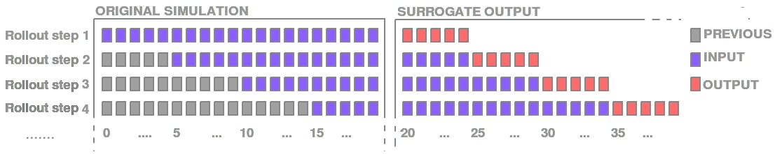
Figure 2: Example rollout using surrogate with $T_{in}=20$ and $T_{out}=5$. For the initial rollout step, the surrogate uses only timesteps from the original simulation, but rollout steps beyond that start using an increasing portion of generated rollout steps.

The starting point of a rollout refers to the timestep at which the predictions from the FNO start. For the results presented here, unless stated otherwise, rollouts begin at $t=20$ for models evaluated on the JOREK datasets and $t=200$ for models evaluated on the STORM dataset. This is to allow for the prior 20 timesteps that are fed to the FNO to generate the predictions and to avoid the turbulance buildup phase for STORM as explained in the STORM section. All reported errors, unless otherwise specified, are computed with min-max normalization applied, as errors without this transformation grow too large and lead to numerical overflow when calculated MSE for longer rollouts.

3.2.4 Transfer learning

Transfer learning was implemented in two stages: (1) the surrogate model was first trained on the full source dataset until convergence, and (2) the model was fine-tuned on the target dataset. During the second stage, the pre-trained model parameters served as the initialization point, replacing the random initialization typically used in training from scratch or during stage 1. When the size of the training dataset was varied, this only affected the amount of data used for fine-tuning dataset. All hyperparameters remained unchanged during fine-tuning, except for gradient clipping, which was adjusted to match the target dataset, and the learning rate, which was set to a lower value. The learning rate was determined through a simple grid search, halving the value until performance ceased to improve, similar to the procedure used for scratch models (described in A.2).

3.2.5 Transfer learning process to new variables

When applying the transfer learning process to new variables in the reduced-MHD JOREK simulation, the procedure was slightly modified. The first two steps were carried out as described above, but using only variables common to both datasets (electric potential and density). An additional step was then added, where the model was fine-tuned a second time on the target dataset (reduced-MHD JOREK), this time using only the variables unique to the target dataset (temperature and current). Although more sophisticated methods exist in the literature for transfer learning, this approach was chosen for this case study for simplicity, with exploration of more advanced techniques left for future work.

4 Results

4.1 Initial results

As a first experiment, FNOs were trained to learn the evolution for each of the three full simulation datasets (electrostatic JOREK, reduced-MHD JOREK and STORM), converging to the test MSE in table 2 (this invovles a rollout of length 5 timesteps meaning no autoregressive rollout and thus no input error). Both the electrostatic JOREK and STORM surrogates were trained on all fields except the auxiliary variables, while reduced-MHD JOREK was trained on all available fields, including the auxiliary variables. The reduced-MHD JOREK model exhibited the largest error overall, and there was significant variation in the one-step error between variables for some models, which could suggest potential overfitting to specific variables over others in the dataset.

Electrostatic JOREK STORM Reduced-MHD JOREK Variable (MSE$\pm$STD) (MSE$\pm$STD) (MSE$\pm$STD) Temperature ($T$) $6.18\pm 4.09\times 10^{-8}$ $2.15\pm 3.31\times 10^{-4}$ Electric potential ($\Phi$) $2.32\pm 2.93\times 10^{-6}$ $2.21\pm 0.492\times 10^{-6}$ $1.07\pm 2.00\times 10^{-4}$ Density ($\rho$) $3.69\pm 5.64\times 10^{-6}$ $9.45\pm 1.73\times 10^{-6}$ $8.27\pm 13.7\times 10^{-5}$ Vorticity ($\omega$) $4.03\pm 7.47\times 10^{-6}$ Magnetic flux ($\Psi$) $3.77\pm 5.23\times 10^{-5}$ Current ($zj$) $9.72\pm 18.3\times 10^{-5}$

Table 2: MSE on mininmum output length (meaning 5 timesteps) for each rescaled dataset variable averaged across different starting points for all dataset trajectories.

Example trajectory rollouts for test samples are shown in figs 3-5. These rollouts are plotted at specific time points for every field showing the target simulation, the learnt surrogate and the absolute error between them. From these figures, it can be seen that the surrogates were able to learn global features, such as the location of the density source in STORM (figure 5) and the location of the blobs in JOREK (figure 3 and 4). However, it is clear that for longer time rollouts the finer details of the fields are quite different from the ground truth. This is shown quantitatively in figures 6- 8, where the rollout errors are calculated as averages across the multiple trajectories in the testing dataset. Notably, for both JOREK models (figures 6 and 7), an error peak is observed for many of the variables. This error peak is not present for STORM in figure 8. To investigate this further, two experimental setups were employed: (1) evaluating the rollout error initiated at various points in the trajectory and (2) assessing the expected error assuming ideal model inputs with no accumulating error. These are discussed in the following subsections.

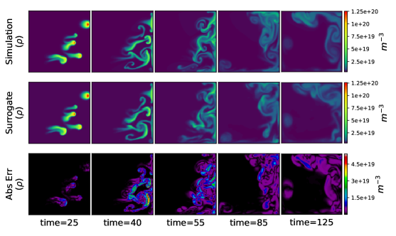
(a) Particle density $\rho$ ($m^{-}3$)

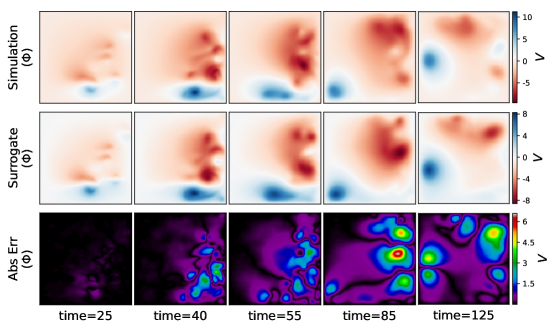
(b) Electric potential $\Phi$ ($V$)

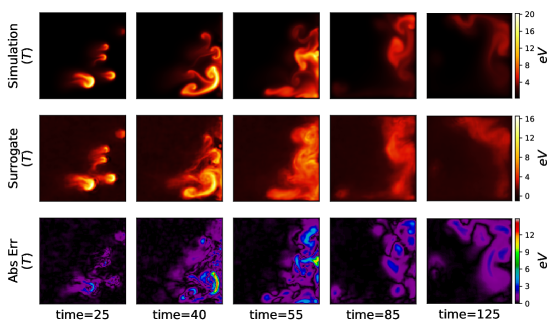
(c) Temperature $T$ ($eV$)

Figure 3: An example electrostatic JOREK run plotted at specific rollout timesteps for fields (a) density, (b) electric potential and (c) temperature.

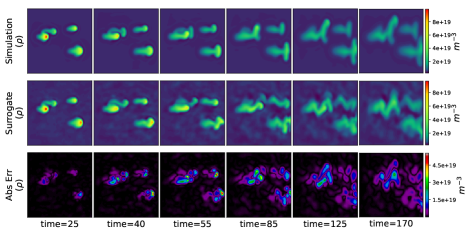
(a) Particle density $\rho$ ($m^{-}3$)

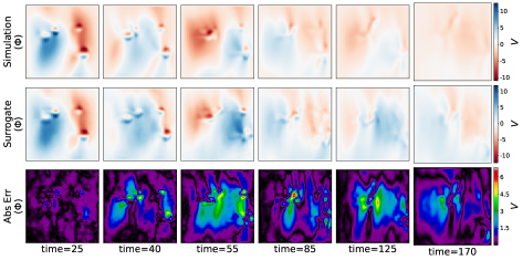
(b) Electric potential $\Phi$ ($V$)

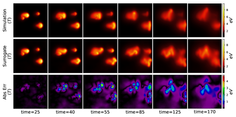
(c) Temperature $T$ ($eV$)

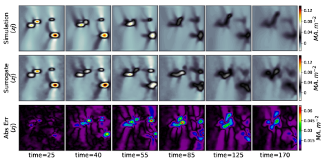
(d) Toroidal current $zj$ ($MA.m^{-2}$)

Figure 4: An example reduced-MHD JOREK run for fields (a) density, (b) electric potential, (c) temperature and (d) current. The remaining fields can be found in the appendix at 16

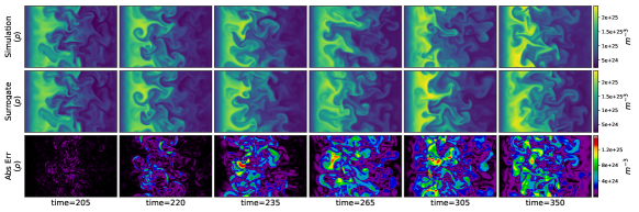
(a) Particle density $\rho$ ($m^{-}3$)

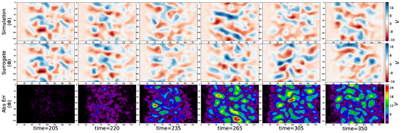
(b) Electric potential $\Phi$ ($V$)

Figure 5: An example STORM run for fields (a) density and (b) electric potential

4.1.1 Impact of trajectory location with JOREK datasets

Distinct behaviors emerged among the three fields in the Electrostatic JOREK model, as seen in fig 6:

1. Electric Potential: Electric potential errors increased steadily over time, closely following the expected pattern of accumulating error. Unlike the other two variables, no trajectory-specific peaks were observed, suggesting that error growth here is primarily due to cumulative error effects over longer rollouts.

2. Temperature: Unlike electric potential, rollout errors for temperature did not consistently increase. Instead, errors decreases throughout the auto-regressive rollout when these rollouts were initiated later in the trajectory. This results in a general pattern where errors are consistently highest at a specific point in the trajectory (around $t=50$) and diminishing in regions further from this point regardless of the time gap since the model last saw the ground truth. These results suggest that temperature error may be predominantly driven by specific trajectory dynamics at that point rather than accumulated input error.

3. Density: The density field showed a combination of both behaviors. When rollouts were initiated prior to $t=50$, a distinct peak appeared in the error profile, similar to the temperature field. However a pattern observed is that this peak diminished and shifted right when rollouts were initiated later in the trajectory. A potential explanation of this can be found if both trajectory-specific dynamics (like in temperature) and accumulating error effects (like in electric potential) are occurring at the same time. When the trajectory is started sooner, the accumulating error has had less time to build and thus the errors introduced by trajectory specific dynamics around $t=50$ are a lot more dominant, causing the error peak to be shifted sooner. Whereas the reverse occurs as the trajectory is started later.

Notably, the observed rollout behavior persisted even when calculating rollout errors solely from target data, removing accumulating input error as a factor (in other words, not running the surrogate in rollout set-up, but just looking at single, short-term predictions). This suggests that there may be a systemic time-dependent issue within the model’s handling of certain fields. This result is similar to [29] where a similar pattern was observed where whilst different models varied significantly in their per-step MSE, they often failed in qualitatively similar regions of the trajectory, suggesting shared limitations in capturing the underlying physics. These weaknesses highlight the need for further refinement of the neural surrogate models, particularly for fields where input error accumulation is not the primary issue but systemic error remains.

For this dataset, having all the variables behave so differently with respect to long rollouts and trajectory locations is particularly puzzling, given that these variables are (1) intrinsically linked within the simulation through the PDE, and (2) modeled together in the same surrogate model. An additional observation is the potential correlation between the size of the error in shorter rollouts and the degree to which accumulating error affects longer rollout behavior. For example, temperature, which exhibits the least error in short rollouts, seems to be less impacted by accumulating error in the autoregressive process. In contrast, electric potential, which shows the most error in short rollouts, is most susceptible to the effects of accumulating error.

For the reduced-MHD JOREK model, a similar pattern was observed, as in fig 7, with an error peak around $t=40$ for most variables, excluding temperature. In contrast to Electrostatic JOREK, error in this model consistently increased over the 10 rollout steps for all fields except magnetic flux. This suggests behavior similar to Eeectrostatic JOREK’s density field, where it is proposed that both influences are in effect. A similar correlation between the size of the error in shorter rollouts and the degree to which accumulating error affects longer rollout behavior is also loosely observed.

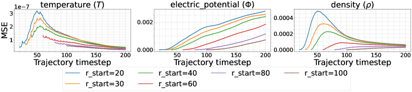
(a) Different starting points with accumulating input error

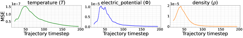
(b) Only ground truth simulation data as input

Figure 6: Long rollout error for FNO model trained on electrostatic JOREK (for each field) for rollout error relative to trajectory timestep (a) with different starting points with accumulating input error and (b) with only ground truth simulation data as input (in other words, not running the surrogate in rollout set-up, but just looking at single, short-term predictions).

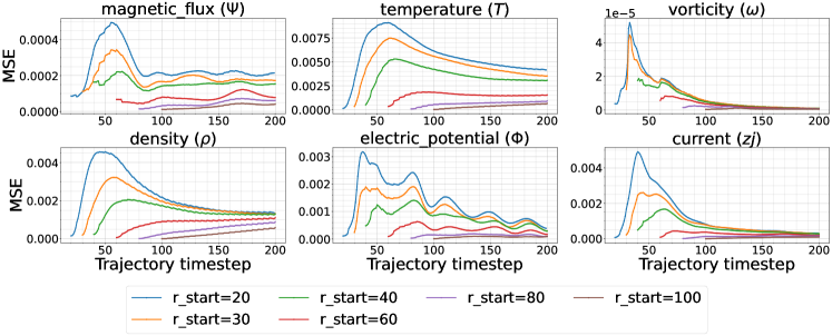
(a) different starting points and accumulating error

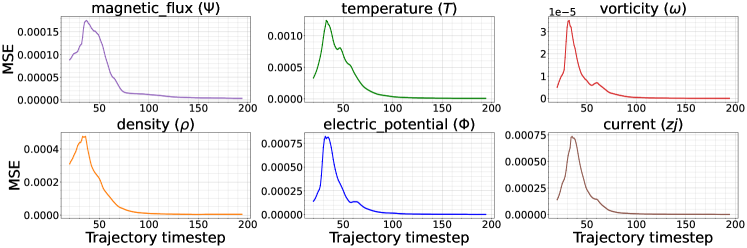
(b) only ground truth simulation data as input

Figure 7: Long rollout error for FNO model trained on electrostatic JOREK (for each field) for rollout error relative to trajectory timestep (a) with different starting points with accumulating input error and (b) with only ground truth simulation data as input (in other words, not running the surrogate in rollout set-up, but just looking at single, short-term predictions).

4.1.2 Impact of trajectory location with STORM dataset

In STORM (seen in fig 8), errors exhibited more uniform patterns across fields:

1. Electric Potential: This field showed an initial exponential error increase, followed by a plateau, suggesting that errors reach a saturation level in longer rollouts. This behaviour was also consistent across different starting points in the trajectory.

2. Density: Density behaved differently, with an initial similar exponential increase followed by a sustained, gradual increase over the rollout duration, indicating no clear saturation point.

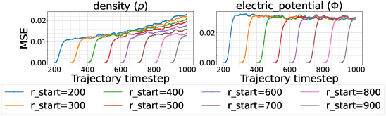
(a) Different starting points with accumulating input error

(b) Only ground truth simulation data as input

Figure 8: Long rollout error for FNO model trained on STORM (for each field) for rollout error relative to trajectory timestep (a) with different starting points with accumulating input error and (b) with only ground truth simulation data as input. (LEFT) is density and (RIGHT) is electric potential.

Unlike both JOREK models, STORM fields did not exhibit trajectory-specific error peaks, pointing to more generalized error accumulation across the rollout.

4.2 Heatflux deposited on the wall

To evaluate the surrogate’s ability to capture key physical behaviors relevant to plasma-facing component performance, the radial heat flux at the wall was computed using the JOREK surrogates. The radial heat flux ($Q_{R}$) quantifies the energy transferred per unit area in the radial direction and is crucial for assessing material stress and component lifetime.

More precisely, the heat flux was computed as:

$$Q_{R}=\rho TV_{R}$$ (4)

where the radial velocity, $V_{R}$, was determined using the relation:

$$v_{R}=R\times B\times\frac{d\phi}{dZ}$$ (5)

where R is the distance in the radial direction, B is the magnetic field and $\frac{d\phi}{dZ}$ is the gradient of the electrostatic potential in the toroidal direction. This assumes a fixed toroidal magnetic field $B=1T$ using the Lorentz force equation for velocity, $v=E\times B$ and accounting for the radial curve. Predictions for the density, electric potential and temperature are produced autoregressively by the surrogate, with the rollout starting at $t=20$. The heat flux on the outmost radial slice across the poloidal direction is considered (which is equivalent to the right hand side boundary as plotted in example fig 3).

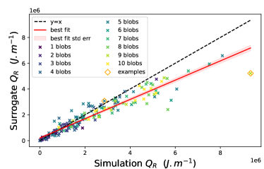
(a) Heatflux scatter plot

(b) Simulation heatflux histogram

Figure 9: (a) Heat flux at boundary integrated over poloidal direction (y-axis) and time comparing surrogate and simulation. Each datapoint is trajectory with the color corresponding to the number of blobs. A black line is an identity line provided as a demonstration of full agreement between surrogate and simulation. The red line is the best fit line with the coefficients ($\pm$stderror): slope $0.75\pm 0.17$ and intercept $2.05\pm 0.47\times 10^{5}$; with a pearson coefficient of $0.95$. The orange diamonds circle the 2 example trajectories shown in the figures below. (b) is the distribution of the simulation heatflux, demonstrating that there are many more trajectories with lower heatflux values

The scatter plot in Figure 9 compares the total heat flux at this boundary, integrated over time and the poloidal direction. The surrogate model performs well for lower heat flux values ($<0.4\times 10^{6}$) but systematically underestimates higher fluxes, with errors increasing as flux rises. This issue is particularly pronounced for extreme cases ($>0.6\times 10^{6}$), though such instances are rare, occurring in only $\sim$5.00% of the trajectories. Similar trends are observed in the reduced-MHD JOREK dataset (see Appendix), though meaningful conclusions are limited due to the small dataset size. A strong trend with the number of blobs simulated is observed, where a higher number of blobs and high heat fluxes are correlated with a general deterioration of the surrogate performance.

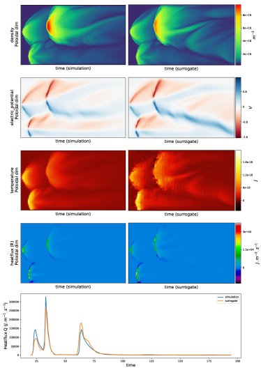
(a) Example 1

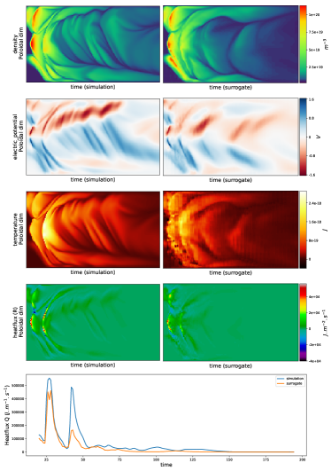
(b) Example 2

Figure 10: Comparison of heat flux over the right-hand side boundary for electrostatic JOREK throughout the rollout. Two example trajectories are shown where the total heat flux is (a) low and (b) high. Each subfigure includes a line plot of the heat flux summed over the boundary, revealing strong agreement in the timing of blob impacts on the wall, which cause spikes in heat flux. However, in (b), the magnitude of the heat flux is notably underpredicted. Additionally, four 2D plots display the spatial and temporal evolution of density, temperature, electric potential, and heat flux across the poloidal boundary, offering a detailed comparison of the two cases.

To illustrate these findings, two example trajectories are shown: one where the integrated heat flux over the wall is low and another where it is high. The integration over the poloidal boundary provides a physically meaningful measure of the total heat load on the wall, helping to assess the model’s predictive accuracy. In the first case, the model correctly captures both the timing and magnitude of heat flux spikes as blobs impact the wall. In contrast, the second example highlights a case where, while the model correctly predicts the timing of two spikes, it consistently underestimates their magnitude. These results reinforce that while the surrogate effectively models typical heat flux behavior, it struggles with high-flux events — likely due to an inadequate learned representation of extreme plasma dynamics. Nonetheless, this analysis provides a useful, physically motivated example of the surrogate’s capabilities that may be adopted in future work.

4.3 Investigation into error spikes in JOREK datasets

In both the Electrostatic and reduced-MHD JOREK datasets, significant error spikes were observed at specific points in the simulation trajectory, independent of accumulated input error. These peaks occurred at around $t=50$ for the electrostatic JOREK model and $t=30$ for the reduced-MHD JOREK model. Notably, trajectories across both JOREK datasets exhibited consistent physical behaviors: blobs were initialized at random positions, traveled to the right, interacted with the boundary, and eventually dissipated. These consistent dynamics suggest that specific physical events occurring at certain points in the trajectory, rather than a gradual accumulation of inaccuracies over time, are likely to be the dominant contributors to the observed rollout error.

Figure 11: FNO model trained electrostatic JOREK rollout examples at different points in time for the (rescaled) density field; demonstrating that the blobs tended to hit the wall around $t=50$.

Figure 12: FNO model trained reduced-MHD JOREK rollout examples at different points in time for the density field; demonstrating that the blobs did not hit the around $t=30$.

This finding is notable because it suggests, somewhat counterintuitively, that input error accumulation is not always the primary driver of performance issues in these datasets for long rollouts. Instead, the errors can also be driven by specific transitions in physical behavior. Many studies on neural operators focus on understanding and improving long-time rollouts accuracy, but this finding highlights that the usual behavior — where errors accumulate steadily over time — is not observed uniformly across all variables. In this case, error accumulation appears significant only for specific variables, such as the electric potential $\phi$ for elecrostatic JOREK, underscoring the importance of analyzing errors in the context of the underlying physical dynamics.

When looking at specific examples, it can be noticed that the error peaked at $t=50$, aligning with blob-wall collisions (fig 11). However, this pattern was absent in reduced-MHD JOREK, where blobs took longer to reach the boundary and dissipated beforehand (fig 4).

Various factors were systematically ruled out, with all being explored for electrostatic JOREK and, where possible, for reduced-MHD JOREK. Analysis of pointwise error for electrostatic JOREK (see A.9) revealed distinct spatial patterns, with errors predominantly concentrated near boundaries, particularly the right-hand side wall during early timesteps.), before spreading to other boundaries over time. This suggests that boundary interactions present a challenge for the neural operator, which lacks explicit boundary condition enforcement beyond observed edge behavior in the dataset. However for reduced-MHD JOREK, the error was not concentrated near the boundary, suggesting additional contributing factors.

Resampling around the error peaks (see A.7, not possible for reduced MHD-JOREK due to its fragmented nature) to improve representation of these dynamics did not enhance performance, suggesting that the issue is not due to under-representation in the training dataset. Furthermore, while the magnitude of error increased with the number of blobs in a trajectory (see A.8 for figures, reduced-MHD JOREK validation dataset was too small with only 2 samples per blob number on average), the timing and frequency of error spikes were not correlated with blob count. Furthermore, the lower MSE observed further into the rollout could be related to a decrease in overall simulation values. However, this hypothesis was discounted, as the error peaks persisted even when switching to percentage error, whether evaluated pointwise or timewise (see A.10 for figures).

Another possible explanation is that the neural operator struggles to capture the rapid acceleration of blobs. This process involves a quick increase in velocity, peaking before the blobs collide with the wall, followed by a fast deceleration during collision and eventual dissipation. Such abrupt transitions in dynamics may be difficult for the FNO to resolve, especially in localized regions. This is consistent with findings in [21], which suggest that these models do not effectively capture fine-scale spatial features. Whilst increasing the input buffer size (which is already reasonably large at $t_{in}=20$) for rollout predictions could potentially improve accuracy by capturing more information about acceleration, it would also introduce inefficiencies in downstream applications, where many timesteps need to be simulated before passing the data to the neural operator. The objective employed may also contribute to the observed error patterns. Mean squared error (MSE), while effective for tracking precise blob positions and localized features, may inadequately capture the more turbulent or diffusive phases where the properties that are more interesting are statistical properties like average heat flux.

Overall, the dynamics behind the observed error spikes remain unclear but these findings highlight the importance of considering both the physical dynamics of the system and the limitations of the model when analyzing long-term predictions.

4.4 Transfer learning

In this section the results on transfer learning are presented. Table 3 provides an overview of the transfer learning case studies, detailing the source and target datasets and variables for each of the cases.

Source Target Case Dataset Variables Dataset Variables 1 Electrostatic JOREK density, electric potential STORM density, electric potential 2 STORM density, electric potential Electrostatic JOREK density, electric potential 3 Electrostatic JOREK density, electric potential Reduced-MHD JOREK density, electric potential 4 Electrostatic JOREK density, electric potential Reduced-MHD JOREK temperature, current

Table 3: The different transfer learning cases investigated for transfer learning. EJOREK is electrostatic JOREK and MJOREK is Reduced-MHD JOREK

4.4.1 Cross-Simulation-Code Transfer learning

For transfer learning between independently developed simulation codes, the adaptability of neural operator surrogates was tested using data from the STORM and JOREK models. These codes simulate distinct physical phenomena and operate under different frameworks, providing a test for cross-simulation-code transfer. The goal was to assess whether models trained on one dataset could effectively transfer knowledge to another, highlighting the potential for cross-simulation-code surrogate modelling in fusion research.

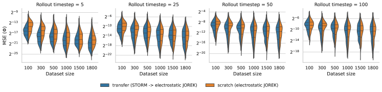
(a) Case 1 Transfer learning from STORM to electrostatic JOREK

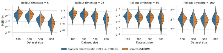
(b) Case 2 Transfer learning from electrostatic JOREK to STORM

Figure 13: Scratch and transfer model error for electric potential at different timesteps and different dataset sizes. The line is the medium error and the error bars correspond to the 16th and 84th percentile.

The details of the two experimental cases (cases 1 and 2) are summarized in table 3. In both scenarios, the MSE was analyzed as a function of dataset size and rollout length. Errors were measured at specific timesteps (e.g., 5, 25, 50, and 100) to assess performance trends over time. As illustrated in figure 13 for electric potential, transfer learning models demonstrated improved performance compared to scratch models for shorter rollouts, particularly when smaller training datasets were used.

However, for longer rollouts, the performance of the transfer learning models progressively converged to similar results with that of the scratch models. Increasing the dataset size improved the performance of both approaches, though this trend became less stable for longer rollouts. A similar pattern was observed across varying dataset sizes: as the dataset size increased, the performance gap between transfer learning and scratch models narrowed. This indicates that transfer learning’s advantage diminishes for extended rollouts.

These findings underscore the need for more robust transfer learning strategies capable of improving long-term rollout accuracy.

4.4.2 Transfer Across Simulation Fidelity Levels in JOREK

The third scenario explored transfer learning between different fidelity levels within the JOREK simulation code, moving from low- to high-fidelity datasets. The objective was to assess whether transfer learning could enable the FNO to leverage lower-fidelity data to enhance performance on higher-fidelity datasets. This approach aimed to reduce the need for generating large high-fidelity datasets, thereby mitigating the computational burden associated with high-fidelity modeling.

The sole case in Table 3 represents this fidelity transfer experiment. Similar to the cross-simulation-code analysis, the MSE error was evaluated against dataset size and rollout length. Compared to the cross-simulation-code results, transfer learning between fidelities yielded more substantial improvements in accuracy for short rollouts, with the improvements diminishing more gradually. For example, in the density field at the smallest dataset size of 3797 slices, transfer learning achieved an error reduction of an order of magnitude for a short rollout (timestep 5), decreasing the MSE from $5.74\times 10^{-4}$ to $7.62\times 10^{-5}$. For a longer rollout (timestep 100), the error reduced by a factor of 2 with the MSE decreasing from $1.13\times 10^{-3}$ to $5.80\times 10^{-4}$. However, this advantage still disappeared for longer rollouts.

The findings demonstrate that transfer learning is most effective when the source and target datasets share considerable similarities. This suggests the potential for a practical pathway for accelerating model training by leveraging cheaper, low-fidelity simulations as a foundation for high-fidelity model development. With this strategy, the computational costs associated with generating large high-fidelity simulation datasets could be drastically reduced.

(a) Density

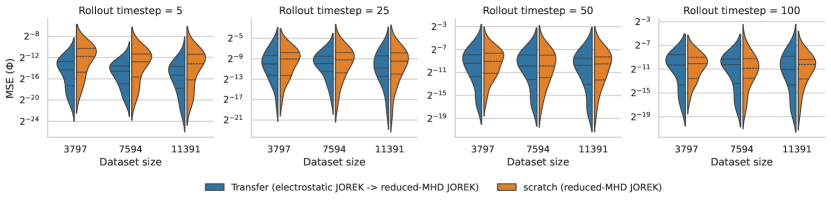
(b) Electric potential

Figure 14: Scratch and transfer model error at different timesteps and different dataset sizes for case 3. Scratch was trained from scratch on the reduced-MHD JOREK dataset whilst transfer model was first trained on electrostatic JOREK and then finetuned on reduced-MHD JOREK. The line is the medium error and the error bars correspond to the 16th and 84th percentile.

4.4.3 Transfering to unseen variables for higher fidelity

A challenge encountered when transferring from low- to high-fidelity JOREK simulations was that the target dataset (reduced-MHD JOREK) contained variables absent in the source dataset (electrostatic JOREK) such as current. Neural operators like the Fourier Neural Operator (FNO) lack the flexibility to seamlessly incorporate prior knowledge from learned variables into datasets with new variables. To address this, a two-step transfer learning approach was devised, as detailed in section 3.2. This method aims to allow the model to transfer learnt information to previously unseen variables in the target datasets previously unseen variables to evaluate applicability as demonstrated in this study using the reduced-MHD JOREK dataset.

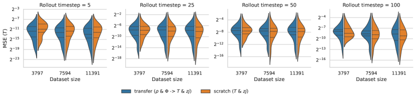
(a) Temperature

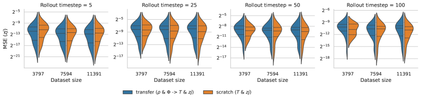
(b) Current

Figure 15: Scratch and transfer model error at different timesteps and dataset sizes on reduced-MHD JOREK. Scratch model was trained directly on the corresponding variables on the dataset. Transfer x2 model was first trained on electrostatic JOREK density and electric potential, finetuned on reduced-MHD JOREK density and electric potential (similar to prior section) and the transferred to reduced-MHD JOREK temperature and current. The line is the medium error and the error bars correspond to the 16th and 84th percentile.

The same error metrics were produced, as illustrated in figure 15. Consistent with previous findings, the transfer models generally outperformed the scratch models during shorter rollouts. However, relative to the previous findings, the performance improvement diminished more rapidly for longer rollouts. In addition, the scratch model consistently demonstrated better average performance than the transfer model in longer rollouts for the temperature field. This pattern suggests that transferring knowledge between variables might improve short-term performance but could also lead to negative transfer effects [47]. This result highlights the need for careful adaptation of transfer learning when working with datasets that involve previously unseen variables.

5 Conclusion

5.0.1 Key Observations

This work demonstrates the potential of neural operators as surrogate models for simulating the evolution of variables in tokamak plasma systems. Fourier Neural Operators were trained using the STORM and JOREK simulation datasets and the surrogate model’s ability to replicate plasma behaviour autoregressively was evaluated for both short and long temporal rollouts.

Key observations and contributions include the following:

1. Impact of Starting Points, Boundary Interactions and long-term degradation: the FNO model’s error patterns are influenced by both accumulating input errors and specific trajectory events, with boundary interactions playing a significant role in the errors observed in the Electrostatic JOREK model, highlighting the importance of considering underlying physical dynamics when evaluating model performance.

2. Transfer Learning for Dataset Efficiency: Given the high computational cost of generating simulation datasets, transfer learning techniques were explored to leverage information across similar and more complex datasets. Results indicate that transfer learning offers a notable improvement when the source and target datasets share physical similarities, such as in cases involving electrostatic and reduced-MHD JOREK datasets. Findings suggest that transfer learning from lower- to higher-fidelity JOREK simulations can be very effective, even in longer rollouts, helping to reduce the computational resources and expert human effort required for generating large databases of high-fidelity simulations. However, transfer learning’s benefits will diminish in longer rollouts, especially when the datasets differed in their underlying physics. This suggests that while transfer learning can be a powerful tool for dataset efficiency, its advantages are more pronounced in shorter rollouts and datasets with similar physical properties.

3. Variable-to-Variable Transfer Challenges: The FNO architecture lacks flexibility to accommodate a varying number of variables, and transferring knowledge to datasets with new variables is not straightforward. To address this, a two-step approach was explored. While this method outperformed models trained from scratch in short rollouts, its performance deteriorated in longer rollouts relatively quickly. This suggests that transferring knowledge between distinct variables governed by different physical processes (e.g., the reduced-MHD JOREK dataset) can suffer from negative transfer effects. These challenges highlight the need for more flexible transfer learning techniques when dealing with datasets that involve varying or previously unseen variables.

5.0.2 Limitations and Future work

While this study represents a step forward in leveraging neural operators for plasma physics simulations, there are several limitations that warrant further investigation.

Only the FNO architecture was explored, which will struggle with complexities such as 3D unstructured meshes or non-standard geometries. Future research should explore alternative architectures, such as attention-based models like the UPT [16], which could improve long-term predictive accuracy and better handle non-overlapping variable sets. Additionally, it is important to consider the role of physical constraints, such as boundary conditions, which may play a key role in stabilizing predictions and preventing errors from escalating over time. Some of the observed performance degradation could be attributed to poor representations of certain physical processes, such as blob acceleration, which future models could better account for.

Although transfer learning provided promising results, particularly for datasets with similar physical properties, the performance gains were short-lived for long rollouts. Future research could explore more sophisticated methods such as LoRA [48] to improve adaptability. Attention mechanisms could also be incorporated to prioritize relevant features during knowledge transfer and strategies like varying learning rates or selectively freezing layers could help identify and keep the parts of the network most responsible for effective transfer.

Additionally, recent advancements, such as the Pushforward Trick [24], PDE-Refiner [21], and autoregressive diffusion models [49], have demonstrated significant potential in enhancing the robustness of neural operators for long-term predictions. These methods use techniques such as refining predictions iteratively, correcting for low-amplitude spatial frequencies, and incorporating input errors directly into the training process as a kind of data augmentation. Such techniques could substantially improve the stability and accuracy of long rollouts. Incorporating these approaches into future models could help overcome the limitations observed in practical applications.

Finally, there is a need to explore the application of neural operators to more complex physics models, such as higher-dimensional or multiphysics simulations. A recent step in this direction was taken by [50] to emulate gyrokinetic simulations. Extending the neural operator framework to these more complex systems could provide valuable insights and significantly improve its practical applicability in fusion research.

In summary, while this work highlights the potential of FNO-based surrogates for plasma physics, there are clear avenues for improvement. By addressing the limitations discussed and integrating recent advancements in neural network architectures and techniques, future research can enhance the reliability, scalability, and versatility of neural operators in fusion research.

Appendix A Appendix

A.1 Simulation hyperparameters

The range of input parameters are as follows for each of the simulation datasets.

Input parameter	Min/max	Type & unit
number of blobs	[1 : 10]	discrete
R-position of blob	[9.6 : 10.4]	continuous [m]
Z-position of blobs	[-0.4 : 0.4]	continuous [m]
width of blobs	[0.02 : 0.1]	continuous [m]
density amplitude of blobs	[0.1 : 0.4]	continuous [$10^{20}m^{-3}$]
temperature amplitude of blobs	[12 : 72]	continuous [eV]

Table 4: The shared input parameter range used for both JOREK datasets.

Input parameter	Min/max	Type & unit
amplitude of density source	[0.05 : 0.5]	continuous [$10^{18}m^{-3}$]
width of density source	[1 : 10]	continuous [1.414213562mm]

Table 5: The input parameter range used for the STORM dataset.

A.2 Model hyparpameters and additional training details

The models were trained on all fields (unless otherwise noted) using a mean squared error (MSE) loss function, optimized over a maximum of 72 hours. The Adam optimizer, with a cosine annealing learning rate scheduler starting at $5\times 10^{-4}$, $2\times 10^{-4}$ and $2\times 10^{-4}$ for electrostatic JOREK, reduced-MHD JOREK and STORM respectively and a minimum of 1.e-7, was used throughout. To determine an optimal learning rate, a small grid search was run for the model trained on each full dataset, halving the learning rate until performance stopped improving. Once selected, this learning rate was consistently applied across all models trained on smaller data subsets.

To enhance training stability, gradient clipping was applied with a standard threshold of $0.125$, apart from electrostatic JOREK which used a value of $0.25$.

All these hyperparameters are described in the tables below.

Name	Value
Model	FNO
FNO modes	32
Num FNO blocks	3 x 1
Hidden channels	128
Activation layer	GeLu
Loss	MSE
Batch size	64
Optimizer	Adam
Learning rate schedular	CosineAnnealingLR
Weight decay	1e-5
Eta min lr	1e-7

Table 6: Hyperparameters consistent between datasets

Name	Electrostatic JOREK	Reduced-MHD JOREK	STORM
Early stopping patience	10	50	10
Gradient clipping val	0.25	0.125	0.125
Input timesteps ($t_{i}n$)	20	5	20
Output timesteps ($t_{o}ut$)	5	5	5
Starting Learning rate	5e-4	5e-4	2e-4
Max epochs	2000	2000	500

Table 7: Hyperparameters different for each datasets

A.3 Example trajectory for additional fields for reduced-MHD JOREK

Example trajectory for additional fields not included in 4.1.

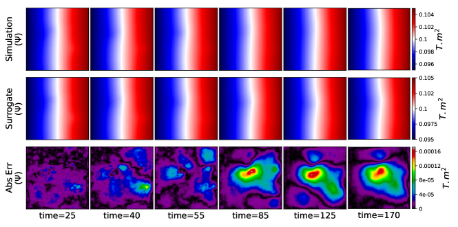
(a) Poloidal magnetic flux $\Psi$ ($T.m^{2}$)

(b) Toroidal vorticity $\omega$

Figure 16: An example reduced-MHD JOREK run for additional fields (a) magnetic flux and (b) vorticity

A.4 MJOREK heatflux

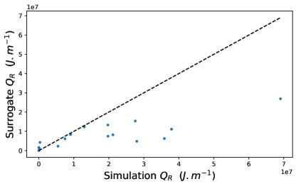
Figure 17: Heatflux at boundary integrated over poloidal direction (y-axis) and time comparing surrogate and simulation. Each datapoint is trajectory. Black lines are reference identity lines $(0,0)$, $(10^{7},0)$ and $(0,10^{7})$

A.5 Cross code transfer learning additional figures

Additional figures for the other field (electrostatic JOREK) discussed in section 4.4.1.

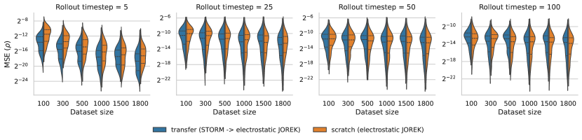
(a) Case 1 Transfer learning from STORM to electrostatic JOREK

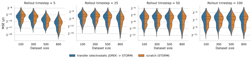
(b) Case 2 Transfer learning from electrostatic JOREK to STORM

Figure 18: Scratch and transfer model error for density at different timesteps and different dataset sizes. The line is the medium error and the error bars correspond to the 16th and 84th percentile.

A.6 Changing t-out

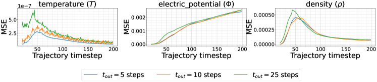
Figure 19: Electrostatic JOREK model rollout error (starting at $t=20$ trained with different number of $t_{out}$ steps.

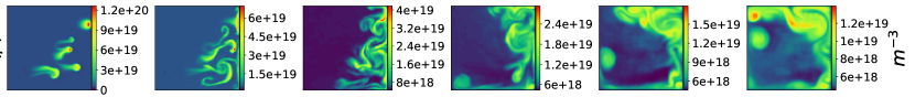
(a) Example rollouts with $t_{out}=5$

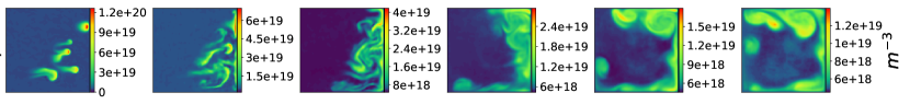
(b) Example rollouts with $t_{out}=10$

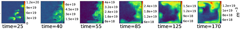
(c) Example rollouts with $t_{out}=25$

Figure 20: Electrostatic JOREK model rollout error trained with different number of $t_{out}$ steps

A.7 Varying sampling of hump region (electrostatic JOREK)

Figure 21: Increased sampling of region between t=30-70 by ensuring that 1-X% of the training sampling was within this region, X being the percentage of samples being completely random. Rollout error with only ground truth simulation data as input (in other words, not running the surrogate in rollout set-up, but just looking at single, short-term predictions).

A.8 Blob number (electrostatic JOREK)

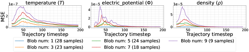
Figure 22: FNO model trained on electrostatic JOREK split according to number of blobs in simulation. Rollout error with only ground truth simulation data as input (in other words, not running the surrogate in rollout set-up, but just looking at single, short-term predictions).

A.9 Pointwise error (JOREK)

Using the model trained on the electrostatic JOREK dataset, analysis of the pointwise error (figure 23 and 24) revealed distinct spatial patterns. Pointwise error involves computing the error at each spatial point for a given time step, then averaging this error across the validation dataset to assess the model’s accuracy across space and time. Errors were predominantly localized near the boundaries, particularly the right-hand side wall during early timesteps. The error peaks at $t=50$, coinciding with the point at which blobs collided with the wall (fig 11). Over time, these localized errors expanded to encompass other boundaries. This spatial distribution suggests that boundary interactions present a challenge for the neural operator. It is important to note that within the neural operator, there is no explicit consideration of boundary conditions, other than the observed behavior at the edges of the spatial dimensions for the simulation in the dataset.

However, this pattern was not observed in the reduced-MHD JOREK dataset, where blobs took a much longer time to travel to the right boundary and diffused or dissipated before hitting it before reaching the boundary (see fig 4 for an example), and the peak error at $t=30$ occurred earlier in the trajectory well before the blobs have hit the right wall (see fig 24). This divergence suggests that boundary effects alone cannot fully explain the observed error spikes, as other factors must be contributing to the dynamics.

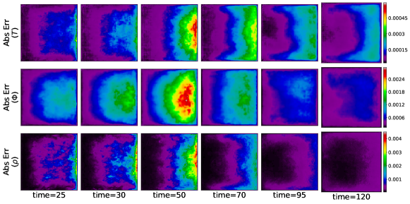
Figure 23: This figure illustrates the pointwise model error for the electrostatic JOREK dataset at specific time steps, averaged across the validation dataset. The results indicate that the error is predominantly concentrated near the boundaries, both during periods of peak error and at other times. This suggests that boundary conditions significantly influence model performance, contributing to localized error accumulation over time. All errors are calculated from the rescaled fields.

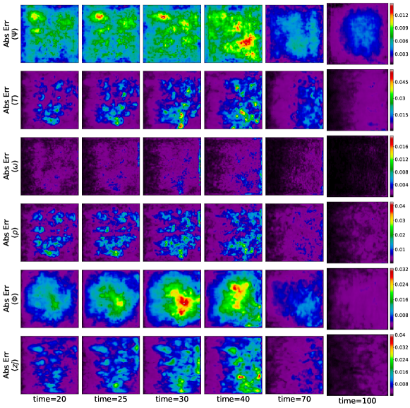
Figure 24: This figure illustrates the pointwise model error for the reduced-MHD JOREK dataset at specific time steps, averaged across the validation dataset. The results indicate that the error is not concentrated near the boundaries unlike electrostatic JOREK. All errors are calculated from the rescaled fields.

A.10 NMSE (JOREK)

• Pointwise normalization error $:=MSE/target$ calculated pointwise. This scales error up according to the size of the target value at each point.

• Timewise (avg) normalization error $:=MSE/avgTarget$ calculated pointwise where avgTarget is the target averaged across spartial dimensions, but keeping the time dimension. This scales error up according to the average taget value at each time.

These are all calculated on the rescaled datasets.

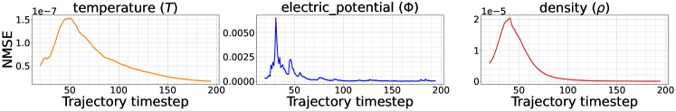
(a) Timewise (avg) normalization

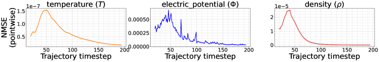
(b) Pointwise normalization

Figure 25: No accumulating error (only simulation input) for FNO model trained on electrostatic. Error is normalized either pointwise, or timewise (avg).

(a) Timewise (avg) normalization

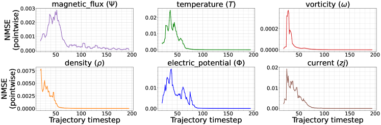
(b) Pointwise normalization

Figure 26: No accumulating error (only simulation input) for FNO model trained on reduced-MHD JOREK split

References

- [1] Alberto Loarte et al. “Chapter 4: Power and particle control” In Nuclear Fusion 47, 2007, pp. S203–S263
- [2] Thomas Eich et al. “Scaling of the tokamak near the scrape-off layer H-mode power width and implications for ITER” In Nuclear Fusion 53, 2013
- [3] Fabio Riva et al. “Three-dimensional plasma edge turbulence simulations of the Mega Ampere Spherical Tokamak and comparison with experimental measurements” In Plasma Phys. Control. Fusion 61.9 IOP Publishing, 2019, pp. 095013
- [4] M. Hoelzl et al. “The JOREK non-linear extended MHD code and applications to large-scale instabilities and their control in magnetically confined fusion plasmas” In Nuclear Fusion 61.6 IOP Publishing, 2021, pp. 065001 DOI: 10.1088/1741-4326/abf99f
- [5] Michele Romanelli et al. “JINTRAC: a system of codes for integrated simulation of tokamak scenarios” In Plasma and Fusion research 9 The Japan Society of Plasma ScienceNuclear Fusion Research, 2014, pp. 3403023–3403023
- [6] S. Wiesen et al. “The new SOLPS-ITER code package” PLASMA-SURFACE INTERACTIONS 21 In Journal of Nuclear Materials 463, 2015, pp. 480–484 DOI: https://doi.org/10.1016/j.jnucmat.2014.10.012
- [7] G L Derks et al. “Benchmark of a self-consistent dynamic 1D divertor model DIV1D using the 2D SOLPS-ITER code” In Plasma Physics and Controlled Fusion 64.12 IOP Publishing, 2022, pp. 125013 DOI: 10.1088/1361-6587/ac9dbd
- [8] G… Huijsmans et al. “Modelling of edge localised modes and edge localised mode control” In Physics of Plasmas 22.2 AIP Publishing, 2015 DOI: 10.1063/1.4905231
- [9] L. Easy et al. “Investigation of the effect of resistivity on scrape off layer filaments using three-dimensional simulations” In Physics of Plasmas 23.1, 2016, pp. 012512 DOI: 10.1063/1.4940330
- [10] A. Stegmeir, T. Body and W. Zholobenko “Analysis of locally-aligned and non-aligned discretisation schemes for reactor-scale tokamak edge turbulence simulations” In Computer Physics Communications 290, 2023, pp. 108801 DOI: https://doi.org/10.1016/j.cpc.2023.108801
- [11] Ernst Hairer, Syvert Norsett and Gerhard Wanner “Solving Ordinary Differential Equations I: Nonstiff Problems”, 1993 DOI: 10.1007/978-3-540-78862-1
- [12] Vignesh Gopakumar and D Samaddar “Image mapping the temporal evolution of edge characteristics in tokamaks using neural networks” In Machine Learning: Science and Technology 1.1 IOP Publishing, 2020, pp. 015006 DOI: 10.1088/2632-2153/ab5639
- [13] Stefan Dasbach and Sven Wiesen “Towards fast surrogate models for interpolation of tokamak edge plasmas” In Nuclear Materials and Energy 34, 2023, pp. 101396 DOI: https://doi.org/10.1016/j.nme.2023.101396
- [14] Nikola Kovachki et al. “Neural Operator: Learning Maps Between Function Spaces”, 2023 arXiv:2108.08481 [cs.LG]
- [15] Zongyi Li et al. “Fourier Neural Operator for Parametric Partial Differential Equations”, 2021 arXiv:2010.08895 [cs.LG]
- [16] Benedikt Alkin et al. “Universal Physics Transformers: A Framework For Efficiently Scaling Neural Operators”, 2024 arXiv: https://arxiv.org/abs/2402.12365
- [17] K.. Plassche et al. “Fast modeling of turbulent transport in fusion plasmas using neural networks” In Physics of Plasmas 27.2 AIP Publishing, 2020 DOI: 10.1063/1.5134126
- [18] A. Ho et al. “Neural network surrogate of QuaLiKiz using JET experimental data to populate training space” In Physics of Plasmas 28.3 AIP Publishing, 2021 DOI: 10.1063/5.0038290
- [19] P Mánek et al. “Fast regression of the tritium breeding ratio in fusion reactors” In Machine Learning: Science and Technology 4.1 IOP Publishing, 2023, pp. 015008 DOI: 10.1088/2632-2153/acb2b3
- [20] Vignesh Gopakumar et al. “Plasma surrogate modelling using Fourier neural operators” In Nuclear Fusion 64.5 IOP Publishing, 2024, pp. 056025 DOI: 10.1088/1741-4326/ad313a
- [21] Phillip Lippe et al. “PDE-Refiner: Achieving Accurate Long Rollouts with Neural PDE Solvers”, 2023 arXiv:2308.05732 [cs.LG]
- [22] Maziar Raissi, Paris Perdikaris and George Em Karniadakis “Physics Informed Deep Learning (Part I): Data-driven Solutions of Nonlinear Partial Differential Equations”, 2017 arXiv: https://arxiv.org/abs/1711.10561
- [23] Vignesh Gopakumar et al. “Plasma Surrogate Modelling using Fourier Neural Operators”, 2023 arXiv:2311.05967 [physics.plasm-ph]
- [24] Johannes Brandstetter, Daniel Worrall and Max Welling “Message Passing Neural PDE Solvers”, 2023 arXiv:2202.03376 [cs.LG]
- [25] S… Pamela et al. “Neural-Parareal: Self-improving acceleration of fusion MHD simulations using time-parallelisation and neural operators” In Computer Physics Communications 307.109391, 2025 DOI: https://doi.org/10.1016/j.cpc.2024.109391
- [26] Jony Castagna and Francesca Schiavello “StyleGAN as a Deconvolutional Operator for Large Eddy Simulations” In Proceedings of the Platform for Advanced Scientific Computing Conference, PASC 2023, Davos, Switzerland, June 26-28, 2023 ACM, 2023, pp. 5:1–5:7 DOI: 10.1145/3592979.3593404
- [27] Jonas M. Mikhaeil, Zahra Monfared and Daniel Durstewitz “On the difficulty of learning chaotic dynamics with RNNs”, 2022 arXiv: https://arxiv.org/abs/2110.07238
- [28] Arieh Iserles “A First Course in the Numerical Analysis of Differential Equations”, Cambridge Texts in Applied Mathematics Cambridge University Press, 2008
- [29] Yoeri Poels et al. “Fast dynamic 1D simulation of divertor plasmas with neural PDE surrogates” In Nuclear Fusion 63.12 IOP Publishing, 2023, pp. 126012 DOI: 10.1088/1741-4326/acf70d
- [30] L. Zanisi et al. “Efficient training sets for surrogate models of tokamak turbulence with Active Deep Ensembles” In Nuclear Fusion 64.3 IOP Publishing, 2024, pp. 036022 DOI: 10.1088/1741-4326/ad240d
- [31] W. Hornsby et al. “Gaussian process regression models for the properties of micro-tearing modes in spherical tokamaks” In Physics of Plasmas 31.1 AIP Publishing, 2024 DOI: 10.1063/5.0174478
- [32] P. Rodriguez-Fernandez et al. “Enhancing predictive capabilities in fusion burning plasmas through surrogate-based optimization in core transport solvers” In Nuclear Fusion 64.7 IOP Publishing, 2024, pp. 076034 DOI: 10.1088/1741-4326/ad4b3d
- [33] Neil Houlsby et al. “Parameter-Efficient Transfer Learning for NLP”, 2019 arXiv: https://arxiv.org/abs/1902.00751
- [34] Colin Raffel et al. “Exploring the Limits of Transfer Learning with a Unified Text-to-Text Transformer”, 2023 arXiv: https://arxiv.org/abs/1910.10683
- [35] Kuniaki Saito, Kohei Watanabe, Yoshitaka Ushiku and Tatsuya Harada “Maximum Classifier Discrepancy for Unsupervised Domain Adaptation”, 2018 arXiv: https://arxiv.org/abs/1712.02560
- [36] Karl R. Weiss, Taghi M. Khoshgoftaar and Dingding Wang “A survey of transfer learning” In Journal of Big Data 3, 2016 URL: https://api.semanticscholar.org/CorpusID:256407097
- [37] Jason Yosinski, Jeff Clune, Yoshua Bengio and Hod Lipson “How transferable are features in deep neural networks?” In Advances in Neural Information Processing Systems 27 Curran Associates, Inc., 2014 URL: https://proceedings.neurips.cc/paper_files/paper/2014/file/375c71349b295fbe2dcdca9206f20a06-Paper.pdf
- [38] Shashank Subramanian et al. “Towards Foundation Models for Scientific Machine Learning: Characterizing Scaling and Transfer Behavior”, 2023 arXiv: https://arxiv.org/abs/2306.00258
- [39] Jayesh K. Gupta and Johannes Brandstetter “Towards Multi-spatiotemporal-scale Generalized PDE Modeling”, 2022 arXiv:2209.15616 [cs.LG]
- [40] N R Walkden, L Easy, F Militello and J T Omotani “Dynamics of 3D isolated thermal filaments” In Plasma Phys. Control. Fusion 58.11 IOP Publishing, 2016, pp. 115010
- [41] S F Smith et al. “Simulations of edge localised mode instabilities in MAST-U Super-X tokamak plasmas” In Nucl. Fusion 60.6 IOP Publishing, 2020, pp. 066021
- [42] Kamyar Azizzadenesheli et al. “Neural operators for accelerating scientific simulations and design” In Nature Reviews Physics 6.5 Springer ScienceBusiness Media LLC, 2024, pp. 320–328 DOI: 10.1038/s42254-024-00712-5
- [43] Maarten V. Hoop, Daniel Zhengyu Huang, Elizabeth Qian and Andrew M. Stuart “The Cost-Accuracy Trade-Off In Operator Learning With Neural Networks”, 2022 arXiv: https://arxiv.org/abs/2203.13181
- [44] Vignesh Gopakumar et al. “Fourier Neural Operator for Plasma Modelling”, 2023 arXiv: https://arxiv.org/abs/2302.06542
- [45] N. Carey et al. “Data efficiency and long term prediction capabilities for neural operator surrogate models of core and edge plasma codes”, 2024 arXiv: https://arxiv.org/abs/2402.08561
- [46] Sifan Wang, Hanwen Wang and Paris Perdikaris “Learning the solution operator of parametric partial differential equations with physics-informed DeepOnets”, 2021 arXiv: https://arxiv.org/abs/2103.10974
- [47] Wen Zhang, Lingfei Deng, Lei Zhang and Dongrui Wu “A Survey on Negative Transfer” In IEEE/CAA Journal of Automatica Sinica 10.2 Institute of ElectricalElectronics Engineers (IEEE), 2023, pp. 305–329 DOI: 10.1109/jas.2022.106004
- [48] Edward J. Hu et al. “LoRA: Low-Rank Adaptation of Large Language Models”, 2021 arXiv: https://arxiv.org/abs/2106.09685
- [49] Georg Kohl, Li-Wei Chen and Nils Thuerey “Benchmarking Autoregressive Conditional Diffusion Models for Turbulent Flow Simulation”, 2024 arXiv: https://arxiv.org/abs/2309.01745
- [50] Gianluca Galletti et al. “5D Neural Surrogates for Nonlinear Gyrokinetic Simulations of Plasma Turbulence”, 2025 arXiv: https://arxiv.org/abs/2502.07469