Unraveling the Geometry of Visual Relational Reasoning
Abstract
Humans and other animals readily generalize abstract relations, such as recognizing constant in shape or color, whereas neural networks struggle. To investigate how neural networks generalize abstract relations, we introduce SimplifiedRPM, a novel benchmark for systematic evaluation. In parallel, we conduct human experiments to benchmark relational difficulty, enabling direct model-human comparisons. Testing four architectures—ResNet-50, Vision Transformer, Wild Relation Network, and Scattering Compositional Learner (SCL)—we find that SCL best aligns with human behavior and generalizes best. Building on a geometric theory of neural representations, we show representational geometries that predict generalization. Layer-wise analysis reveals distinct relational reasoning strategies across models and suggests a trade-off where unseen rule representations compress into training-shaped subspaces. Guided by our geometric perspective, we propose and evaluate SNRloss, a novel objective balancing representation geometry. Our findings offer geometric insights into how neural networks generalize abstract relations, paving the way for more human-like visual reasoning in AI.
Introduction
Humans and other animals demonstrate a remarkable ability to identify and generalize abstract relations across diverse contexts. For example, recognizing the relation “constant” allows individuals to flexibly apply it to different attributes, such as a row of objects sharing the same color or shape. Furthermore, one can readily apply the same abstract relation to novel attributes never encountered before. This ability to generalize abstract relations underpins flexible reasoning, supports complex problem-solving, and enables intelligent behavior in novel situations.
A central challenge in cognitive neuroscience and artificial intelligence is to develop neural network models that can achieve similar abstract relation generalization. The Raven’s Progressive Matrices (RPM) task is a widely used benchmark for assessing abstract relational reasoning ability (?). In this task, participants view a grid of images with the bottom-right panel missing. The goal is to identify the relational rules that govern the grid and select the correct missing panel based on these inferred rules. Inspired by this task, researchers have developed large-scale RPM-style datasets, such as Procedurally Generated Matrices (PGM) (?) and the Relational and Analogical Visual rEasoNing (RAVEN) dataset (?, ?), and have trained various neural architectures to solve them (?, ?, ?, ?, ?, ?, ?, ?, ?, ?, ?, ?, ?). While many of these models achieve high test accuracy on the relational rules they are trained on, they struggle to generalize to unseen rules (?). The absence of human behavioral data on the same generalization tasks measured in neural networks further complicates the interpretation of existing results.
This limitation raises a fundamental question: What mechanisms enable or constrain abstract relation generalization in neural networks? While prior studies have documented performance levels, the representational factors shaping generalization remain poorly understood. In particular, it is unclear how learned representations encode relational structure, how these representations differ across neural network architectures, and what geometric constraints govern generalization.
In this work, we introduce a geometric framework to systematically analyze the structure of relational representations in neural networks. To compare quantitatively network generalization performance against humans, we introduce a new benchmark, the Simplified Raven’s Progressive Matrices (SimplifiedRPM) task. Using this benchmark, we compare four representative neural networks spanning different reasoning strategies. ResNet-50 (?), Vision Transformer (?), Wild Relation Network (?), and Scattering Compositional Learner (SCL) (?). We conduct human experiments, concluding that SCL aligns most closely with human relational reasoning.
SimplifiedRPM enables applying a geometric theory (?) originally developed for generalization in visual object classification tasks to the reasoning domain. Specifically, we propose that the reasoning performance of neural networks can be attributed to the geometry of their emergent “rule manifolds”. We demonstrate that this geometric theory precisely predicts empirical generalization error in neural networks, establishing a direct link between the geometry of rule manifolds for unseen relations and generalization performance. Our analysis highlights two key geometric factors, signal and dimensionality, which interact to determine the generalizability of a network. Importantly, we observe a trade-off between signal and dimensionality, driven by a structured compression mechanism, where networks amplify the signal by constraining all class manifolds—including unseen ones—into a low-dimensional subspace spanned by the principal components of the training rules. Motivated by this theory, we introduce SNRloss, a new network training objective explicitly designed to optimize the representation geometry and show that this loss function leads to adequate generalization performance with balanced geometric features. Overall, this work provides new insights into the mechanisms underlying relational reasoning through the lens of representation geometry.
Evaluating Deep Neural Networks in Relational Reasoning
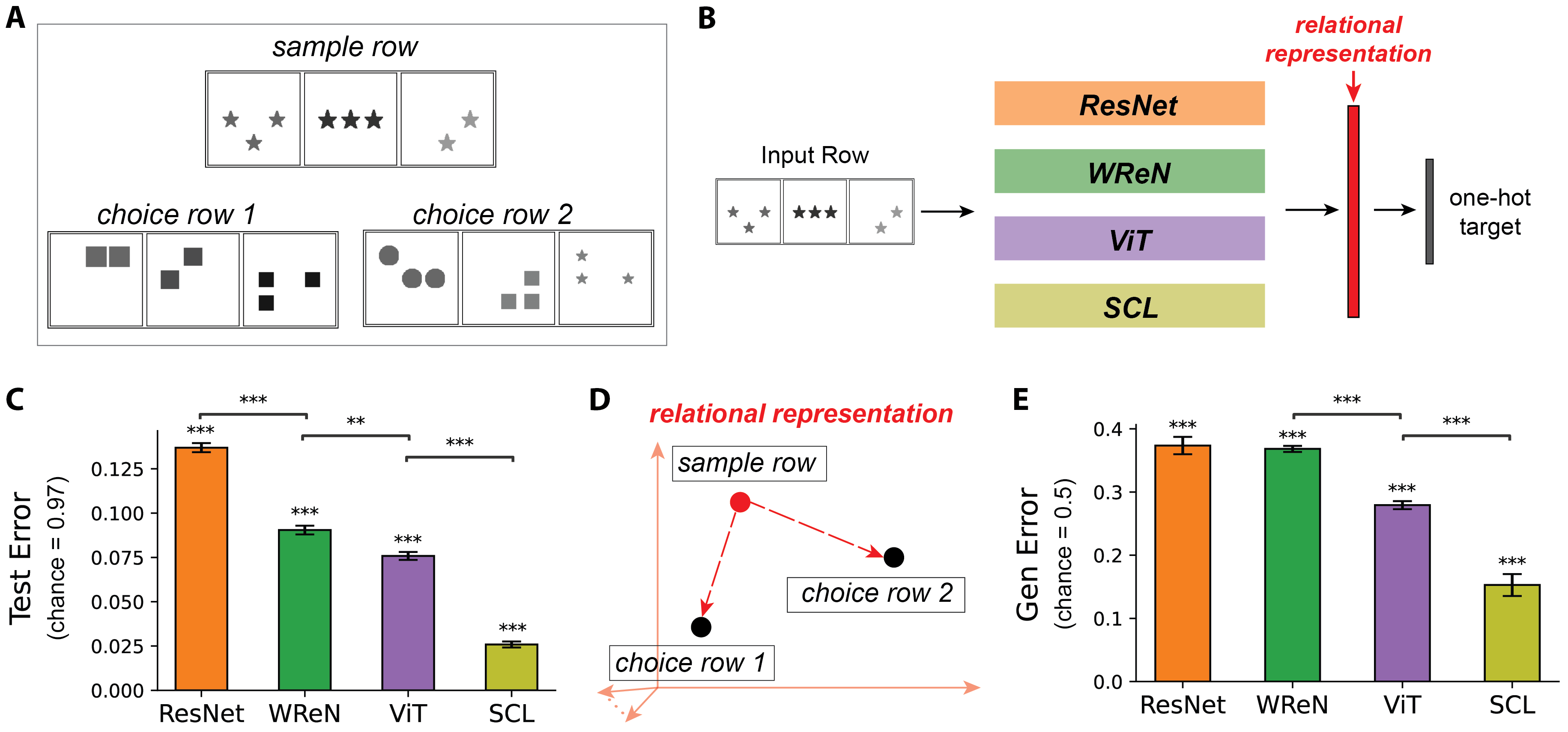
To systematically assess neural networks’ ability to generalize abstract relations, we developed the Simplified Raven’s Progressive Matrices (SimplifiedRPM) task (Fig. 1A). Inspired by the original RPM task (?), SimplifiedRPM requires models to infer a relational rule from a sample row (Fig. 1A, top) and determine which of two choice rows (Fig. 1A, bottom) follows the same rule. Each row consists of three panels with abstract objects, such as triangles or circles, arranged according to a relational rule. For example, the sample row in Fig. 1A illustrates the “constant shape” rule, where all objects share the same shape while other attributes, such as number or position, vary. SimplifiedRPM refines the original RPM task (?) by reducing answer choices from eight to two, mitigating selection bias exploitation (?), and presenting a single example row instead of two to remove multi-row comparisons. These changes maintain RPM’s core challenge while enabling a more focused assessment of relational reasoning.
We construct a dataset for evaluating abstract relation generalization in the SimplifiedRPM task, comprising rows governed by 40 distinct relational rules. Each rule applies an abstract relation (e.g., constant) to an object attribute (e.g., shape). The abstract relations and attributes are selected to be consistent with those used in human experiments (?, ?) while maximizing the number of rules for comprehensive evaluation. Importantly, each row corresponds to a unique rule. We generate many rows per rule, resulting in a dataset of 400k training rows, 40k validation rows, and 40k test rows. To construct a SimplifiedRPM task trial, a sample row is selected that follows one rule. A correct choice is drawn from the same rule, while an incorrect choice is drawn from a different rule. Further details are provided in the Methods section.
We assess models’ ability to generalize abstract relations using a held-out rule split, where out of relational rules are excluded from training. During training, models learn relational structures from the remaining rules. For instance, a model trained on ”constant number” and ”OR shape” may never encounter ”constant shape.” After training, their performance is evaluated on the five withheld rules using the SimplifiedRPM task. This design addresses limitations in the existing RPM benchmarks. RAVEN (?) lacks a split where some test rules are entirely unseen during training. Although PGM’s Held-out Triplet split withholds certain rules, test rows still combine seen and unseen rules, allowing models to rely on familiar rules. In contrast, SimplifiedRPM enforces a strict separation between training and test rules, ensuring a more rigorous evaluation of relational generalization. By systematically varying which rules are withheld, our benchmark provides a comprehensive assessment of models’ ability to generalize across different types of abstract relations.
We evaluate four representative models on the SimplifiedRPM task: ResNet-50 (?) and ViT (?), two benchmark vision models, and WReN (?) and SCL (?), which are explicitly designed for relational reasoning. These models employ different computational strategies: ResNet-50 applies a series of convolutional layers across all panels simultaneously, WReN computes pairwise panel relationships and aggregates them to infer underlying rules, ViT leverages self-attention to capture relational dependencies, and SCL employs a shared relational module to improve abstract relation recognition across object attributes. Together, these models represent diverse approaches to solving RPM tasks. All models are randomly initialized and trained end-to-end. Further details on the model architecture and hyperparameters are provided in the Methods section.
The models process a row to generate a high-dimensional relational representation of its underlying relational rule (Fig. 1B). To train the models on relational rules, we appended a linear classification layer to the relational representations and optimized them end-to-end using cross-entropy loss with one-hot rule labels. Fig. 1C shows test errors across random training and held-out rules splits. All models successfully learned the relational rules, achieving test errors well below the chance level of . Among them, SCL achieved the lowest test error, followed by ViT, WReN, and ResNet-50.
We assess the trained models’ ability to generalize abstract relations to unseen rules using the SimplifiedRPM task. For each pair in the five held-out rules, we generate trials by randomly selecting a sample row that follows one rule, pairing it with a correct choice from the same rule and an incorrect choice from a different rule. In each trial, the model is sequentially presented with the sample row, followed by the two choice rows. The model computes the Euclidean distance between the relational representation of the sample row and each choice row. A trial is deemed correct if the correct choice row is closer to the sample row than the incorrect one (Fig. 1D). All models outperformed the chance generalization error of (Fig. 1E). Among them, SCL achieved the lowest generalization error, followed by ViT, WReN, and ResNet. Notably, SCL also outperformed the other models on the PGM benchmark’s held-out rule split (?), aligning with our observed generalization order.
SCL Captures Human-like Differential Relational Rule Difficulties
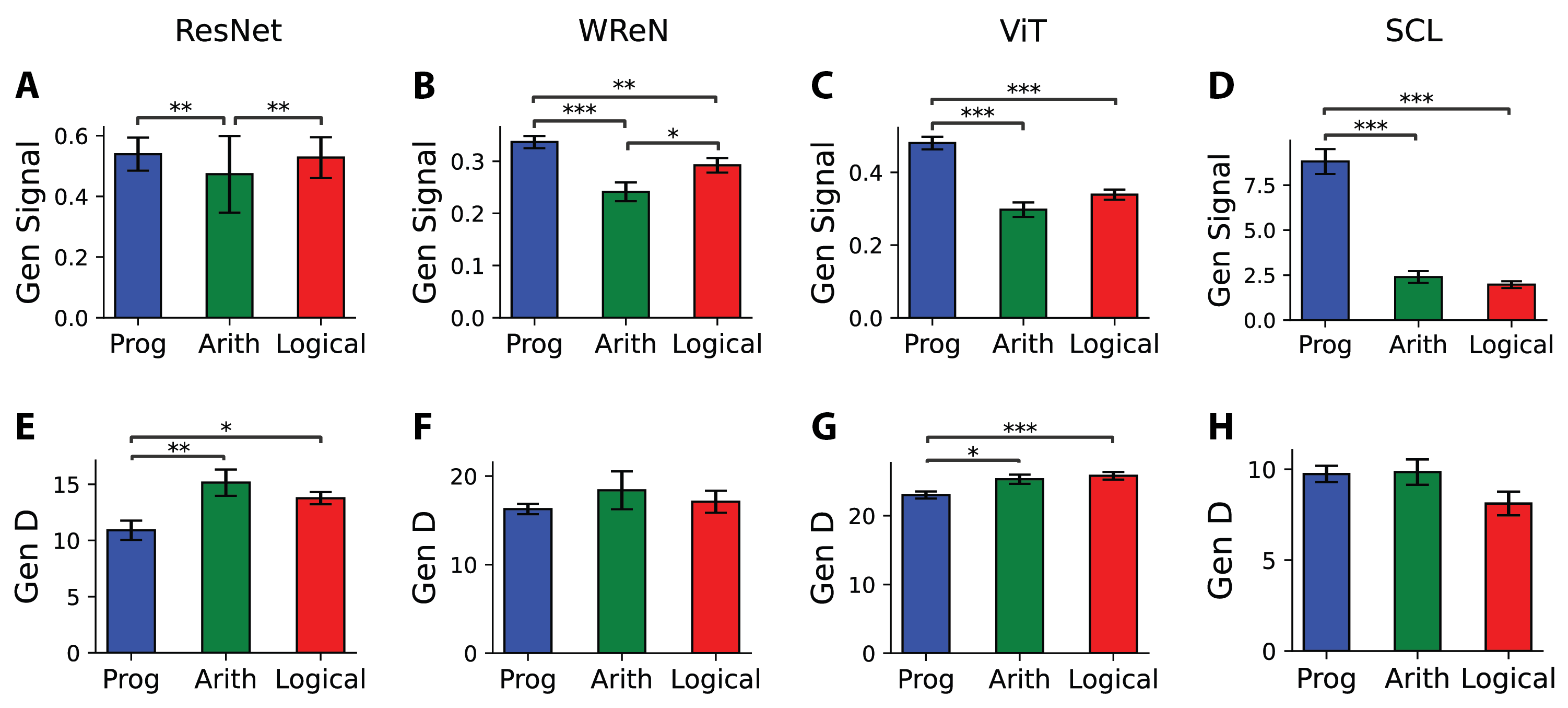
Analyzing only the averaged generalization error is insufficient to fully assess neural networks’ ability to generalize abstract relations, as a model may perform well overall but struggle with rules of specific relation types. To gain deeper insight, we analyzed generalization errors separately for trials where the correct rule of the sample row fell into one of three abstract relation types: progression, arithmetic, or logical. We observed distinct error patterns across models (Fig. 2A-D). ResNet had higher errors for arithmetic than logical rules (Fig. 2A). WReN showed the highest errors for arithmetic, performing worse than progression and logical rules (Fig. 2B). ViT struggled most with arithmetic, while logical rules had higher errors than progression (Fig. 2C). In contrast, SCL showed similarly high errors for arithmetic and logical rules but significantly lower errors for progression (Fig. 2D).
Interestingly, while arithmetic rules posed the greatest challenge for models to generalize, this difficulty did not arise from poor learning of the rules. Instead, it highlights the model’s inability to generalize the arithmetic relation to new attributes. When evaluating test errors—the classification error on novel rows following the trained rules—arithmetic rules consistently had much lower errors than logical rules, which exhibited the highest errors across models (figure S1).
Human performance on the original RPM task (?) follows a hierarchy of difficulty, with progression rules the easiest and logical rules the hardest (?, ?, ?, ?). Unlike models, humans do not receive explicit training on these rules before taking the task (?, ?). To evaluate whether models exhibit human-like reasoning, we compare their ability to generalize to novel rules against human performance.-Among the models examined, only the SCL model replicates the human difficulty pattern across relation types (Fig. 2D). To more rigorously test this alignment, we conducted additional human studies using the SimplifiedRPM task, which allows a direct comparison of abstract relation generalization between humans and models.
To encompass a range of task difficulties, we sampled trials of the SimplifiedRPM task, spanning relational rule pairs with questions per pair. We recruited MTurk participants, each of whom answered randomly selected questions from this pool to minimize sequential learning effects. Participants had unlimited time to respond and were compensated based on accuracy. For each trial, we recorded both accuracy and response time (see Methods for details). Human participants exhibited a mean task error of (means.e.m.), significantly lower than the chance level of (one-sample t-test, , ). The detailed rule pairs included in the human experiment and their corresponding human performance are in table S2.
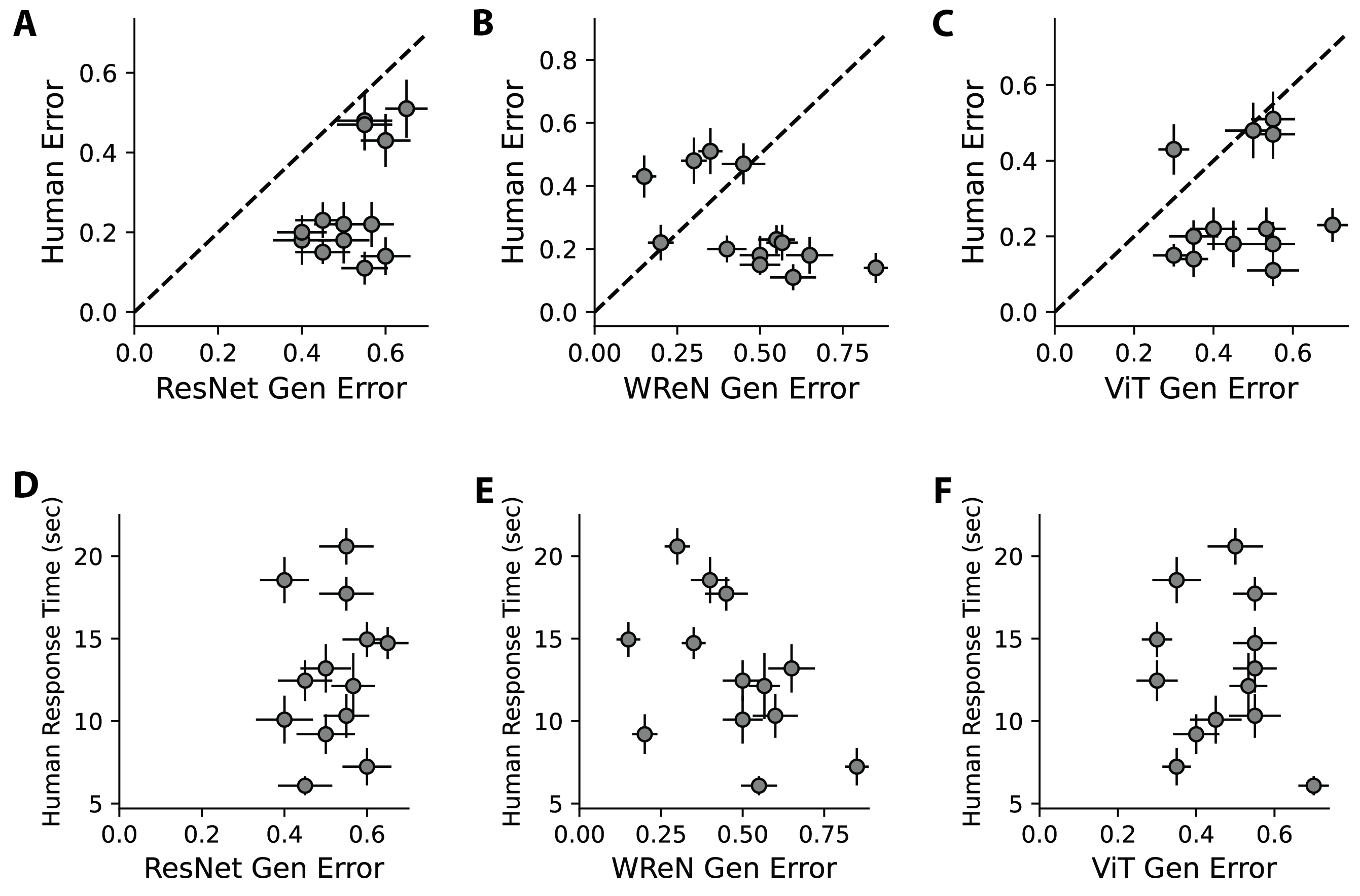
We evaluated the generalization errors of the SCL model on the same SimplifiedRPM trials used in human experiments. Specifically, we trained ten SCL models for each of the thirteen rule pairs, each using a different split of the forty rules in the dataset while ensuring that the target rule pair was always among the five held-out rules. We then measured the generalization error on the held-out pair using the same trials as those used in the human evaluation. The model achieved an average task error of (means.e.m.), close to the human performance. Across the thirteen rule pairs, SCL models exhibited error patterns that correlated with those observed in human participants (Spearman’s rank correlation, , ) (Fig. 2E).
Besides task errors, human response times—the total duration participants spent on each trial—were also strongly correlated with SCL generalization error across the thirteen rule pairs (Spearman’s rank correlation, , ) (Fig. 2F). This finding suggests that participants allocated more time to solving trials that the model found more challenging. In summary, although trained solely to classify relational rules without explicit human-like guidance, the SCL model successfully captures the human order of difficulty. In contrast, other models deviate from human performance patterns (figure S2). This alignment of SCL with human performance motivates further exploration of the mechanisms underlying how neural networks perform relational reasoning.
Geometric Theory of Rule Manifolds Accurately Predicts Error in the SimplifiedRPM Task
To investigate how neural networks achieve relational reasoning and generalize their learned representations to unseen relational rules, we leveraged a geometrical theory of few-shot learning (?). This theory provides a framework for linking errors in the Simplified RPM task to interpretable geometric properties of the relational representations.
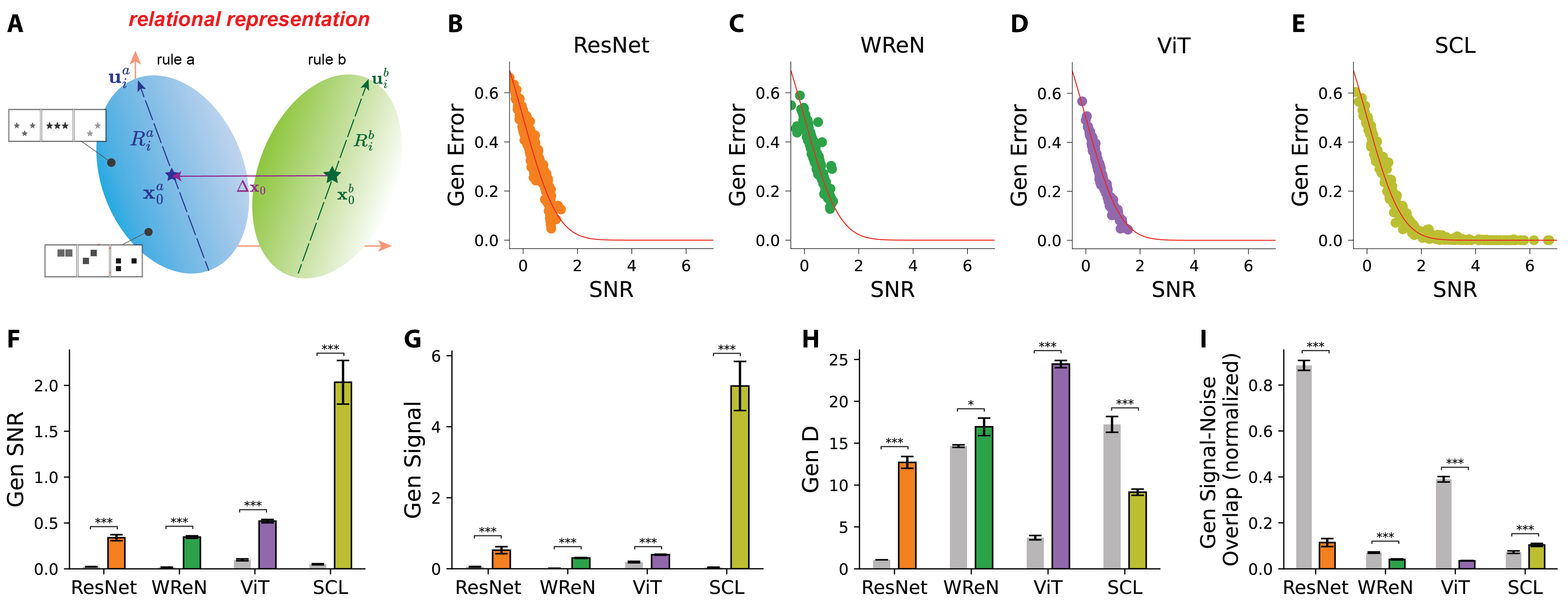
We define rule manifolds as the set of relational representations for rows that follow a specific rule (Fig. 3A). For a rule pair , we consider the average generalization error on the SimplifiedRPM task across all trials where the sample and correct choice rows follow rule , while the incorrect choice row follows rule . Geometrically, corresponds to the probability that a correct choice sampled from the rule a manifold is closer to an incorrect choice from the rule b manifold than to another correct choice from the rule a manifold.
Each rule manifold is defined by its centroid (depicted as blue and green stars in Fig. 3A), which represents the mean position of all representations that follow a given rule. The spread of representations within a manifold is captured by a set of principal axes (illustrated as blue and green dashed arrows in Fig. 3A), along which the variation is quantified by corresponding radii . Here, , where denotes the total dimensionality of the relational representation space. The overall magnitude of this variation is measured by the mean squared radius given by: .
Although the rule manifolds may have complex shapes, the geometrical theory predicts that generalization error can be accurately estimated using only a few key geometric properties. Specifically, the generalization error, , for a given rule pair (,) is governed by the signal-to-noise ratio , following: . Here, is the Gaussian tail function defined as . Higher values correspond to lower generalization errors. The dominant terms of are given by:
| (1) |
The depends on four key interpretable geometric terms. The first is the signal: , which measures the squared Euclidean distance between the centroids of the two rule manifolds (depicted as purple line in Fig. 3A), normalized by the mean squared radius of rule . A larger signal indicates greater separation between the rule and rule manifold centroids, leading to higher and lower generalization error. We denote as the signal direction. The second term is the bias, , which captures the relative difference in the sizes of two rule manifolds. When rule manifold is larger than manifold , the bias term is negative, predicting a lower for rule a. The third term, , represents the inverse of the dimensionality of the rule manifold. , known as the ”Participation ratio” (?), is defined as . quantifies the number of dimensions along which the manifold varies significantly. Higher-dimensional manifolds are preferred for minimizing generalization errors. The last term, signal-noise overlap, is given by and . Here, and are matrices of the manifold axes of variation. The signal-noise overlap quantifies the alignment between these axes of variation and the signal direction . Smaller overlaps result in lower generalization errors.
We estimate the SNR for each model by first extracting the relational representations of rows associated with each held-out rule, thereby forming the rule manifolds. We then computed the geometric properties of these manifolds and calculated the SNR for each held-out rule pair using Equation 1. Fig. 3B-E presents the computed SNR along with the empirically measured generalization error on the SimplifiedRPM task, highlighting close alignments between theoretical predictions (red lines) and empirical results (individual points) across all four models. This alignment validates the geometrical theory as a principled framework for understanding abstract relation generalization through representation geometry.
The geometrical theory identifies three independent mechanisms that facilitate generalization: increasing signal, expanding dimensionality (D), and reducing signal-noise overlap. These mechanisms provide a structured framework for analyzing differences in generalization performance across models. Fig. 3F-I illustrates the geometry of held-out rule representations before (gray bars) and after (colored bars) training, highlighting key differences between models.
Across all models, training increases the SNR for held-out rules (Fig. 3F). When analyzing individual mechanisms, we observe that all models show an increase in signal, with SCL exhibiting a particularly pronounced rise (Fig. 3G). Model-specific differences emerge in dimensionality: ResNet, WReN, and ViT increase D, whereas SCL exhibits a decrease (Fig. 3H). For signal-noise overlap, we normalize the overlap by signal magnitude: . This normalization allows us to distinguish whether a high signal-noise overlap is due to a large signal magnitude or a genuine alignment between the manifold and the signal direction. We observed that ResNet, WReN, and ViT reduce overlap, whereas SCL shows an increase (Fig. 3I). In summary, ResNet, WReN, and ViT leverage all three mechanisms—enhancing signal strength, expanding D, and reducing overlap—to improve generalization. In contrast, SCL primarily relies on increasing signal strength but does so at the cost of reduced dimensionality and increased overlap.
Previously, we observed that different abstract relations—progression, arithmetic, and logical—exhibited varying levels of generalization error across models (Fig. 2A-D). To understand these differences, we examined the role of signal, dimensionality, and overlap in shaping generalization performance.
Across all models, signal strength emerged as the primary driver of generalization performance, with higher signal correlating with lower generalization error. In the SCL model, we observed a human-like generalization pattern where progression rules had significantly lower generalization errors than arithmetic and logical rules (Fig. 2D). This was explained by progression rules exhibiting the highest signal (Fig. 4D). A similar pattern was observed in other models, each exhibiting distinct generalization error trends. In ResNet, arithmetic rules’ errors were higher than logical rules due to lower signal (Fig. 4A). In WReN, arithmetic rules had the highest error, driven by the lowest signal (Fig. 4B). In ViT, progression rules had the lowest error, reflecting their highest signal (Fig. 4C).
Beyond signal, dimensionality (D) did not consistently correlate with generalization performance (Fig. 4E-H). In ResNet and ViT, progression rules had the lowest D despite their low errors, suggesting that D alone does not determine generalization ability. Signal-noise overlap also showed no significant difference across abstract relations (figure S3).
Layer-wise Geometric Analysis Reveals Model-Specific Generalization Strategies
We observed that models exhibit distinct geometries in their relational representations. A key question is how these geometries emerge: Do they form abruptly at specific layers or gradually across the network? To address these questions, we examined the evolution of representational geometry across layers, aiming to pinpoint where abstract relations are extracted and how architecture shapes representation.
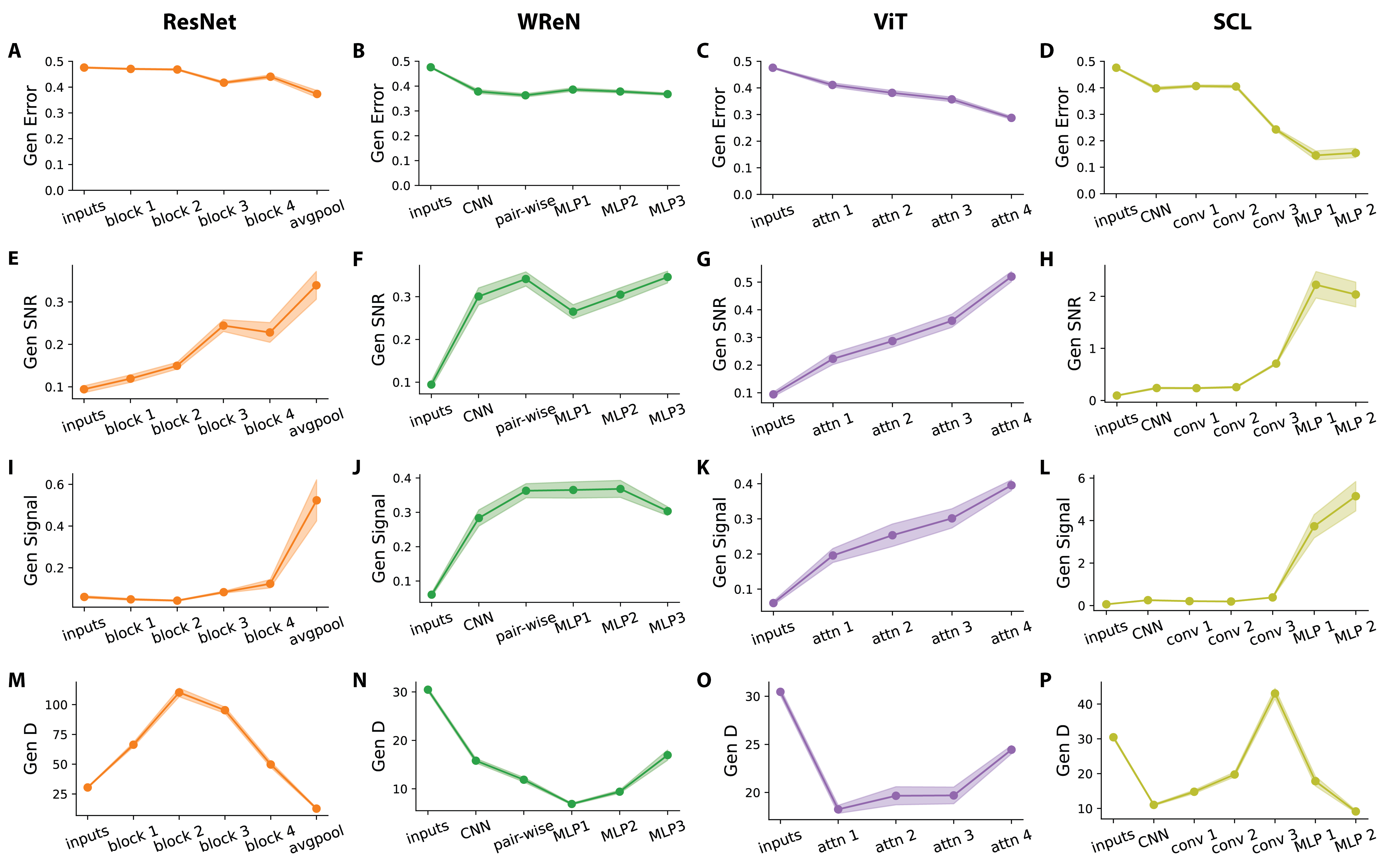
Fig. 5A-D shows each model’s generalization error across layers. At the input stage, rows exhibit a generalization error of , close to the chance level. This suggests the rules are not yet separated at the row pixel level. Across all four models, generalization errors decrease along the layers, demonstrating progressive refinement of relational representations. Fig. 5E-H shows generalization SNR across layers, highlighting distinct relational development patterns across architectures. ResNet-50 and ViT exhibit a gradual increase in SNR, reflecting a steady accumulation of relational information (Fig. 5E,G). In contrast, WReN plateaus early at the pairwise aggregation layer, with later MLP layers failing to improve further generalization SNR (Fig. 5F). In the SCL model—which achieved the best generalization performance—we observed a sharp increase in generalization SNR at the first MLP layer (Fig. 5H).
To gain deeper insights into how relational rule separability evolves across network layers, we decompose SNR into the dynamics of its geometric terms at each layer. While signal generally increases across layers, its layerwise trend does not always follow that of SNR. While SNR steadily rises in ResNet, the signal remains relatively stable until a sharp increase in the final average pooling layer (Fig. 5I). In WReN, the signal plateaus at the pairwise aggregation layer and even decreases in the final MLP layer (Fig. 5J). In ViT, the signal progressively increases across layers (Fig. 5K). In SCL, the signal only begins to rise sharply in the first MLP layer, whereas SNR increases earlier in the last convolutional layer. Furthermore, while the signal rises in the second MLP layer, SNR unexpectedly decreases (Fig. 5L).
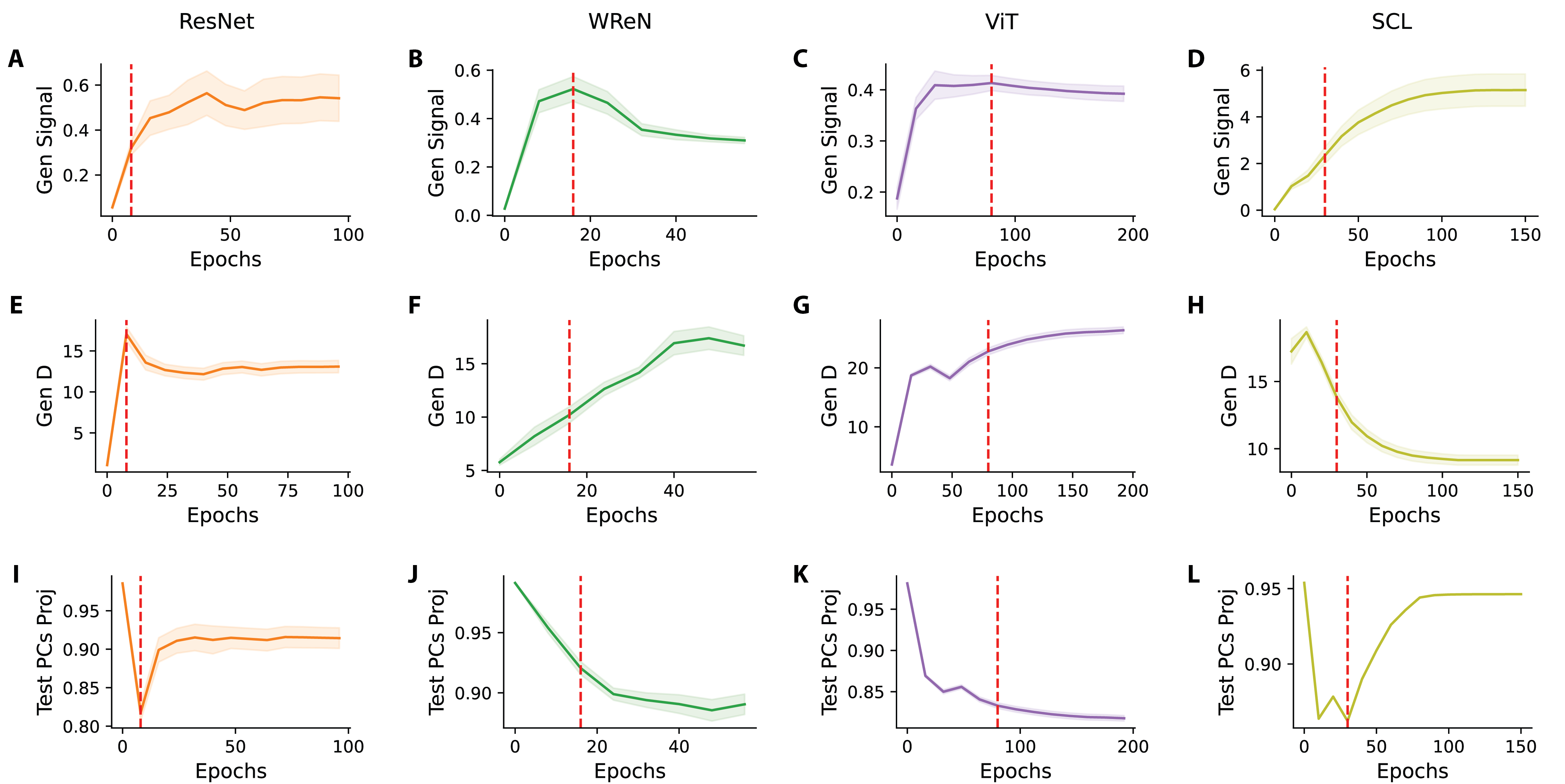
The observed misalignment suggests that signal amplification alone is not sufficient to explain rule separation across layers. To further investigate, we examine the evolution of dimensionality (D) (Fig. 5M-P). Interestingly, unlike the signal, D exhibits a non-monotonic trajectory across layers. ResNet-50 initially expands D in early layers before compressing in later layers (Fig. 5M). WReN follows a different pattern, initially compressing D through pairwise aggregation and early MLP layers before expanding it in later MLP layers (Fig. 5N). ViT maintains a consistently low D throughout, with only a slight increase in the final attention block (Fig. 5O). SCL increases D through convolutional layers but then sharply compresses it in MLP layers (Fig. 5P). These variations in D help explain the gaps observed between signal and SNR evolution through layers. In ResNet-50, the initial expansion of D accounts for the early rise in SNR, which occurs before the signal increases. In SCL, the sharp compression of D in the last MLP layer explains why SNR does not increase alongside the signal.
Across different models, our findings on layerwise geometry suggest that relational abstraction is not a uniform process; each model employs a distinct strategy. The SCL model achieves the best generalization performance by maximizing signal amplification, especially in MLP1, outperforming all other models. In contrast, ResNet-50 and ViT progressively refine relational representations, whereas WReN reaches an early plateau, indicating a bottleneck in relational generalization. While the previous section showed weaker correlations between D and rule separation across abstract relation types, the layerwise analysis reveals a more dynamic interaction. Specifically, D plays a crucial role in shaping relational representations across model layers by refining the effectiveness of signal amplification in driving their emergence.
Structured Compression Drives the Trade-off Between Generalization Signal and Dimensionality
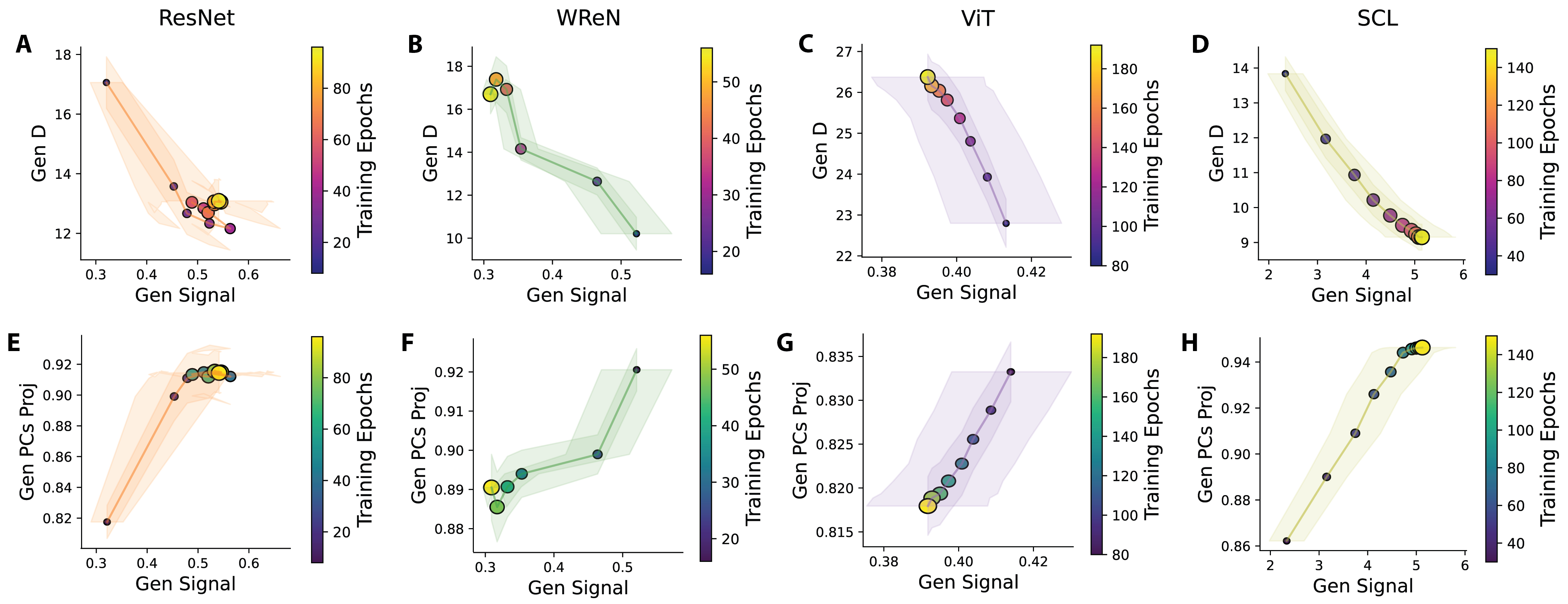
The geometrical theory suggests that high signal and dimensionality (D) benefit generalization. However, we observed that in model layers where significant signal increases occur, D tends to decrease (e.g., Fig. 5I, M for ResNet-50; Fig. 5L, P for SCL). This relationship between the generalization signal and D occurs not only across model layers but also throughout training. In all four models, signal and D exhibit a consistent anti-correlation, with signal increases accompanied by decreases in D (Fig. 6A-D). Intuitively, signal and D are two independent geometric properties. For example, the centroids of two rule manifolds can remain fixed, preserving the signal, while their shapes evolve, changing D. This raises a key question: Why does this trade-off between the generalization signal and D consistently emerge?
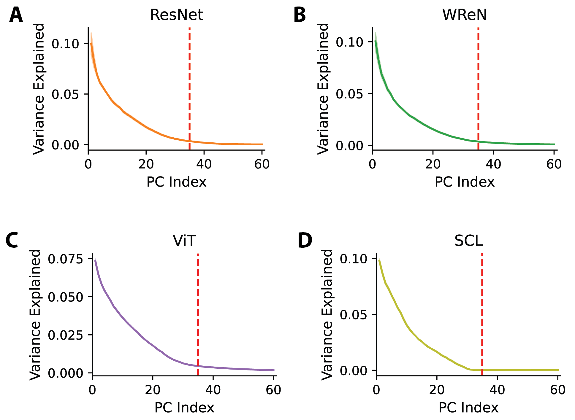
We propose that the trade-off between the generalization signal and D arises from a structured compression effect. All class manifolds—including those for held-out rules—gradually align with a low-dimensional subspace defined by the principal components of the training rules. Across models, the representations of the 35 training rules consistently occupy a low-dimensional space. Notably, we observe a drop in variance explained by the top principal components (PCs) at exactly , matching the number of training rules (figure S4). We hypothesize that the network amplifies the generalization signal by aligning all representations, including those of held-out classes, within this low-dimensional space.
To test this hypothesis, we measured the fraction of variance explained by the top principal components (PCs) of the training rules for each held-out rule manifold. Higher values indicate more substantial alignment with the low-dimensional subspace of training rules. We observed that as the network signal increases, this alignment becomes more pronounced across models (Fig. 6E-H).
Our findings suggest that the observed signal-D trade-off is not incidental but a consequence of structured compression. As networks enhance the generalization signal, they constrain representations into a low-dimensional subspace, prioritizing inter-class signal at the expense of dimensionality. This effect is a general mechanism across different architectures.
Theory-Grounded SNR Loss Yields Geometry-Balanced Representations
Can the geometry predicted by the theory directly guide neural network training? We hypothesize that enforcing this geometry provides a principled approach to learning relational representations. To test this hypothesis, we introduce the SNR loss—an SNR-based objective function that explicitly enforces the predicted geometry.
Specifically, the SNR loss maximizes the SNR for the training rule pairs, reinforcing the optimal representation geometry. We sample rows from relational rules for each input batch and process them through the model to obtain high-dimensional relational representations. The SNR loss is then formulated as:
| (2) |
Here, represents the estimated SNR ( Equation 1) for the ordered rule pair , averaged across all possible rule pairs in the batch.
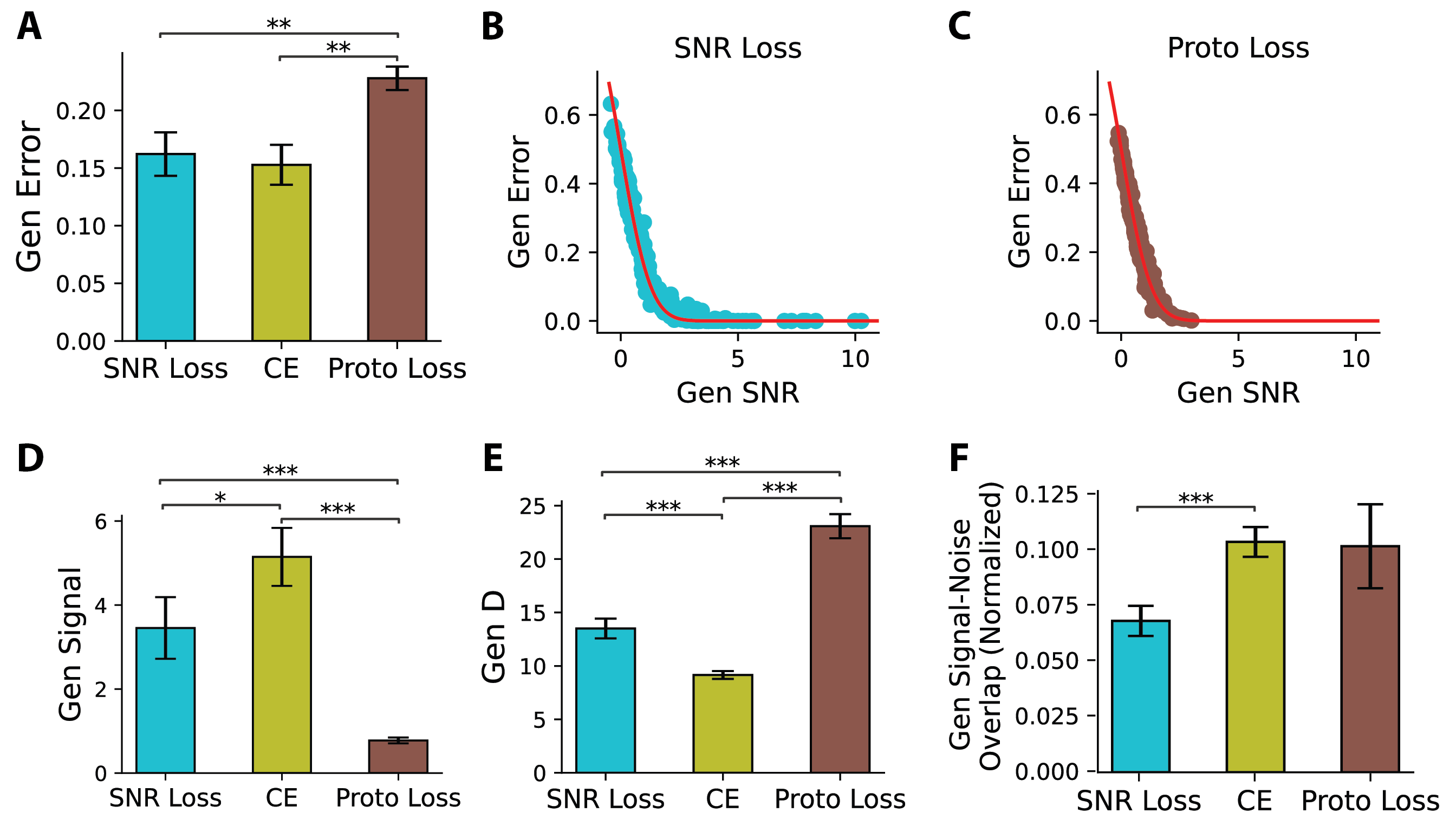
To assess the effectiveness of the proposed SNR loss, we trained the top-performing SCL model using this objective and evaluated its generalization across the same rule splits previously used for training with cross-entropy loss. The model effectively optimized the training rule representations, achieving an average SNR of (means.e.m.) across training rule pairs, as evaluated on novel test rows of the training rules. More importantly, the model effectively separated held-out rules, yielding an averaged generalization error of (means.e.m.) (Fig. 7A). This performance was statistically indistinguishable from models trained with cross-entropy (CE) loss using one-hot rule labels (Wilcoxon signed-rank test: statistic = , , n.s.), confirming that SNR loss achieves competitive generalization while structuring learned representations according to theoretical predictions.
To further evaluate the efficacy of SNR loss, we compared its performance against Prototypical loss, a widely used loss function designed to learn structured representations that generalize to unseen classes (?). Prototypical loss operates by embedding inputs into a high-dimensional representation space and forming class prototypes, defined as the centroids of the representations corresponding to each class. The loss function then encourages representations of samples from the same class to cluster around their respective prototypes. Additional details on Prototypical loss are provided in the Supplementary Text. We trained the SCL model using Prototypical loss on the same rule splits. The resulting model exhibited a generalization error of , significantly higher than that obtained with SNR loss (Fig. 7A). These findings suggest that while both loss functions promote structured representations, SNR loss is more effective in shaping a geometric representation that enhances generalization.
Notably, the generalization errors of models trained with both SNR loss and Proto loss, similar to our previous observations with cross-entropy loss (Fig. 3E), are also accurately predicted by the geometrical theory (Fig. 7B,C). Compared to cross-entropy (CE) and Prototypical loss, SNR loss is uniquely grounded in geometric theory, explicitly accounting for key representation geometries, including signal strength, dimensionality, and signal-noise overlap. This theoretical foundation raises the question of whether SNR loss yields a more advantageous representational geometry relative to other loss functions. To investigate this, we analyzed the representation geometries induced by different loss functions. Our findings show that representations learned with SNR loss have higher dimensionality than those trained with CE loss (Fig. 7E), addressing the low-dimensionality issue in CE training while maintaining relatively high signal strength (Fig. 7D). Furthermore, SNR loss reduces signal-noise overlap, which is beneficial for generalization (Fig. 7F). Although Prototypical loss also encourages high-dimensional representations, it results in the lowest signal, contributing to its worst generalization performance (Fig. 7D, E). These findings highlight that SNR loss shapes the representations of held-out rules in a way that explicitly adheres to geometric principles.
Discussion
We address the fundamental question of how neural networks discover unseen rules when learning abstract relational rules. We hypothesize that networks trained to perform reasoning tasks generate good representations even for unseen rules. The utility of these representations can be quantified by the geometry of the rule manifolds defined by all representations associated with a given rule. Extending the geometric theory of object manifold (?) to abstract rules, we predicted an explicit relation between the generalization performance in visual reasoning and key geometric properties: manifold radii, dimensionality, the distance between manifold centroids, and the overlap between these distances and their subspaces of variation.
To test whether the geometric theory developed for object recognition can be applied to visual reasoning tasks, we introduce SimplifiedRPM, a subset of Raven’s Progressive Matrices (RPM), whose simpler design allows a systematic study of generalization ability in visual reasoning and direct comparison with the above theory. Using this dataset, we trained state-of-the-art deep network architectures (ResNet (?), WReN (?), ViT (?), SCL (?)). We demonstrated the superiority of the SCL (Scatter Compositional Learner) architecture, consistent with previous reports (?). We then conducted an in-depth comparison between the performance of the SCL network and human participants on the same task. Surprisingly, we found excellent agreement between human and network performance, both in terms of overall performance but also across different abstract rules.
Leveraging on a geometrical theory of manifolds initially applied to object recognition tasks (?), we show that interpretable representation geometries can explain models’ performance. Further analysis reveals how different architectures balance signal and dimensionality to achieve relational reasoning while identifying bottlenecks limiting their performance. Building on these insights, we propose SNRloss, a theoretically grounded objective function that explicitly optimizes representation geometry. This novel loss function provides adequate training and generalization capabilities. Our work establishes a geometrically informed framework for analyzing neural networks’ capacity to recognize and generalize abstract relations.
A key insight from our study is that neural networks do not generalize equally well across all abstract relations. While prior research has examined abstract relation generalization in neural networks (?), our work offers a more fine-grained empirical evaluation. Notably, the top-performing model, SCL, aligns closely with human difficulty rankings, with logical rules being the hardest. In contrast, the other three models struggle to generalize arithmetic rules despite achieving high test accuracy. Furthermore, we find that signal, rather than dimensionality or signal-noise overlap, is the primary factor governing these generalization differences among abstract relations. These insights suggest that future models could benefit from strengthening signals for specific relational types.
The best-performing model, SCL, shows a sharp improvement in relational separability only in the last two MLP layers of the network. The earlier layers exhibit only minor gains despite the network being trained end-to-end. This observation suggests that high-level relational abstractions do not gradually build up over the model’s layers but instead emerge abruptly during the final transformations. Geometrically, the signal rises even later in the last MLP layer, while the dimensionality shows a non-monotonic trend—first expanding and then decreasing. The same geometric trend was previously observed in vision models, including ResNet-50, VGG19, and ResNet-152, trained on the ImageNet object classification task (?). The consistency of these geometric trends across models trained on relational reasoning and object classification tasks suggests that they are not merely artifacts of specific architectures or tasks but may reflect a general mechanism of hierarchical abstraction. In contrast, ViTs show a more gradual refinement of relational separation and a steady signal increase across network layers. This indicates that attention mechanisms may support relational learning differently than convolution-based architectures such as SCL and ResNet.
According to the geometrical theory, higher dimensionality should be favorable for generalization. On the other hand, prior studies suggest that low-dimensional manifolds offer advantages for object recognition, enabling the classification of a greater number of objects (?, ?). This contrast implies that dimensionality should not be universally maximized or minimized but instead tuned to task demands. Our findings extend this idea by showing that generalization depends not only on dimensionality but mostly on its interaction with pairwise manifold signals. Specifically, we demonstrate that deep networks systematically compress representations into structured, low-dimensional spaces—even for unseen rules. Moreover, this phenomenon is consistently observed across diverse architectures (e.g., ResNet, SCL), indicating that it is a fundamental learning property rather than an artifact of any specific architecture. We observe that late layers play a crucial role in compressing relational representations, a phenomenon consistent with prior work showing that deep networks tend to refine and condense information in later stages of learning (?). These findings open new avenues to explicitly leverage this signal versus dimensionality trade-off to improve generalization.
Among the tested models, SCL best replicates the human-like difficulty ordering across rules. While prior research has relied on explicit relational priors to achieve human alignment (?), our results demonstrate that SCL, when trained end-to-end on the task, exhibits human-like performance without requiring such priors. Furthermore, SCL’s generalization errors closely correlate with human response times. This raises a key question: What insights does SCL offer for understanding the brain’s relational reasoning mechanisms? The SCL network parallels the brain’s hierarchy: its CNN-based feature extractor mimics the ventral visual cortex, capturing basic features like shape and color (?, ?, ?, ?), while its later reasoning module reflects higher cortical areas supporting relational reasoning (?, ?, ?, ?). We propose that the brain encodes rules of input rows through distinct, rule-specific neural manifolds. Our observation of layer-wise changes in the geometry of these rule manifolds offers hypotheses into how neural representations evolve across brain regions (?, ?). According to the SCL model, early visual areas exhibit high representational dimensionality (D) but low signal, whereas later regions show larger signals with reduced dimensionality. These predictions can be empirically tested by measuring neural activity during abstract reasoning tasks (?, ?, ?, ?).
This study aimed to study the generalization of abstract relations. While the humans in our experiment were not explicitly trained on the rules, their reasoning abilities could be considered ”pre-trained” through life experiences, as they may have previously encountered similar rules. In contrast, neural networks were trained under strictly controlled rule splits, ensuring they had no prior exposure to the rules evaluated for generalization. To address this discrepancy, a crucial next step is to develop a new benchmark for human reasoning that incorporates abstract relations unlikely to have been encountered. Such a benchmark would disentangle relational generalization from prior experience, providing a clearer view of their distinct roles in human abstract reasoning. This approach enables a direct comparison between humans and neural networks, offering deeper insights into their generalization mechanisms.
In summary, our findings not only advance our understanding of relational reasoning in neural networks but also provide testable hypotheses on how geometric principles may underlie abstract reasoning in the brain. Looking forward, our approach opens exciting opportunities for extending geometric analysis to a broader range of cognitive tasks, including real-world visual reasoning benchmarks and cross-modal linguistic challenges.

References and Notes
- 1. J. C. Raven, Mental tests used in genetic, The performance of related indiviuals on tests mainly educative and mainly reproductive. MSC thesisUniv London (1936).
- 2. D. Barrett, F. Hill, A. Santoro, A. Morcos, T. Lillicrap, Measuring abstract reasoning in neural networks, in International conference on machine learning (PMLR) (2018), pp. 511–520.
- 3. C. Zhang, F. Gao, B. Jia, Y. Zhu, S.-C. Zhu, Raven: A dataset for relational and analogical visual reasoning, in Proceedings of the IEEE/CVF conference on computer vision and pattern recognition (2019), pp. 5317–5327.
- 4. S. Hu, Y. Ma, X. Liu, Y. Wei, S. Bai, Stratified rule-aware network for abstract visual reasoning, in Proceedings of the AAAI Conference on Artificial Intelligence, vol. 35 (2021), pp. 1567–1574.
- 5. Y. Wu, H. Dong, R. Grosse, J. Ba, The scattering compositional learner: Discovering objects, attributes, relationships in analogical reasoning. arXiv preprint arXiv:2007.04212 (2020).
- 6. T. W. Webb, I. Sinha, J. D. Cohen, Emergent symbols through binding in external memory. arXiv preprint arXiv:2012.14601 (2020).
- 7. T. W. Webb, et al., The relational bottleneck as an inductive bias for efficient abstraction. Trends in Cognitive Sciences (2024).
- 8. X. Steenbrugge, S. Leroux, T. Verbelen, B. Dhoedt, Improving generalization for abstract reasoning tasks using disentangled feature representations. arXiv preprint arXiv:1811.04784 (2018).
- 9. M. Hersche, M. Zeqiri, L. Benini, A. Sebastian, A. Rahimi, A neuro-vector-symbolic architecture for solving Raven’s progressive matrices. Nature Machine Intelligence 5 (4), 363–375 (2023).
- 10. N. Rahaman, et al., Dynamic inference with neural interpreters. Advances in Neural Information Processing Systems 34, 10985–10998 (2021).
- 11. C. Zhang, et al., Learning algebraic representation for systematic generalization in abstract reasoning, in European Conference on Computer Vision (Springer) (2022), pp. 692–709.
- 12. C. Zhang, et al., Learning perceptual inference by contrasting. Advances in neural information processing systems 32 (2019).
- 13. C. Zhang, B. Jia, Y. Zhu, S.-C. Zhu, Human-level few-shot concept induction through minimax entropy learning. Science Advances 10 (16), eadg2488 (2024).
- 14. S. S. Mondal, J. D. Cohen, T. W. Webb, Slot abstractors: Toward scalable abstract visual reasoning. arXiv preprint arXiv:2403.03458 (2024).
- 15. M. Małkiński, J. Mańdziuk, Deep learning methods for abstract visual reasoning: A survey on raven’s progressive matrices. arXiv preprint arXiv:2201.12382 (2022).
- 16. K. He, X. Zhang, S. Ren, J. Sun, Deep residual learning for image recognition, in Proceedings of the IEEE conference on computer vision and pattern recognition (2016), pp. 770–778.
- 17. A. Dosovitskiy, An image is worth 16x16 words: Transformers for image recognition at scale. arXiv preprint arXiv:2010.11929 (2020).
- 18. B. Sorscher, S. Ganguli, H. Sompolinsky, Neural representational geometry underlies few-shot concept learning. Proceedings of the National Academy of Sciences 119 (43), e2200800119 (2022).
- 19. L. B. V. Matzen, M. W. Van der Molen, A. C. Dudink, Error analysis of Raven test performance. Personality and Individual Differences 16 (3), 433–445 (1994).
- 20. A. Forbes, An item analysis of the advanced matrices. British Journal of Educational Psychology 34 (3), 223–236 (1964).
- 21. P. A. Carpenter, M. A. Just, P. Shell, What one intelligence test measures: a theoretical account of the processing in the Raven Progressive Matrices Test. Psychological review 97 (3), 404 (1990).
- 22. L. E. Matzen, et al., Recreating Raven’s: Software for systematically generating large numbers of Raven-like matrix problems with normed properties. Behavior research methods 42 (2), 525–541 (2010).
- 23. J. Te Nijenhuis, O. F. Voskuijl, N. B. Schijve, Practice and coaching on IQ tests: Quite a lot of g. International Journal of Selection and Assessment 9 (4), 302–308 (2001).
- 24. J. R. Flynn, Massive IQ gains in 14 nations: what IQ tests really measure. Psychological bulletin 101 (2), 171 (1987).
- 25. P. Gao, et al., A theory of multineuronal dimensionality, dynamics and measurement. BioRxiv p. 214262 (2017).
- 26. J. Snell, K. Swersky, R. Zemel, Prototypical networks for few-shot learning. Advances in neural information processing systems 30 (2017).
- 27. U. Cohen, S. Chung, D. D. Lee, H. Sompolinsky, Separability and geometry of object manifolds in deep neural networks. Nature communications 11 (1), 746 (2020).
- 28. S. Chung, D. D. Lee, H. Sompolinsky, Classification and geometry of general perceptual manifolds. Physical Review X 8 (3), 031003 (2018).
- 29. R. Shwartz-Ziv, N. Tishby, Opening the black box of deep neural networks via information. arXiv preprint arXiv:1703.00810 (2017).
- 30. D. R. Little, S. Lewandowsky, T. L. Griffiths, A Bayesian model of rule induction in Raven’s Progressive Matrices, in Proceedings of the annual meeting of the cognitive science society, vol. 34 (2012).
- 31. D. J. Freedman, M. Riesenhuber, T. Poggio, E. K. Miller, A comparison of primate prefrontal and inferior temporal cortices during visual categorization. Journal of Neuroscience 23 (12), 5235–5246 (2003).
- 32. Y. Yamane, K. Tsunoda, M. Matsumoto, A. N. Phillips, M. Tanifuji, Representation of the spatial relationship among object parts by neurons in macaque inferotemporal cortex. Journal of neurophysiology 96 (6), 3147–3156 (2006).
- 33. G. Kreiman, Biological and Computer vision (MIT Press) (2021).
- 34. A. Nayebi, R. Rajalingham, M. Jazayeri, G. R. Yang, Neural foundations of mental simulation: Future prediction of latent representations on dynamic scenes. Advances in Neural Information Processing Systems 36 (2024).
- 35. T. Davis, M. Goldwater, J. Giron, From concrete examples to abstract relations: The rostrolateral prefrontal cortex integrates novel examples into relational categories. Cerebral Cortex 27 (4), 2652–2670 (2017).
- 36. M. V. Chafee, B. B. Averbeck, D. A. Crowe, Representing spatial relationships in posterior parietal cortex: single neurons code object-referenced position. Cerebral Cortex 17 (12), 2914–2932 (2007).
- 37. C. Summerfield, F. Luyckx, H. Sheahan, Structure learning and the posterior parietal cortex. Progress in neurobiology 184, 101717 (2020).
- 38. S. Nelli, L. Braun, T. Dumbalska, A. Saxe, C. Summerfield, Neural knowledge assembly in humans and neural networks. Neuron 111 (9), 1504–1516 (2023).
- 39. L. McIntosh, N. Maheswaranathan, A. Nayebi, S. Ganguli, S. Baccus, Deep learning models of the retinal response to natural scenes. Advances in neural information processing systems 29 (2016).
- 40. M. Genkin, K. V. Shenoy, C. Chandrasekaran, T. A. Engel, The dynamics and geometry of choice in premotor cortex. BioRxiv (2023).
- 41. T. A. Engel, X.-J. Wang, Same or different? A neural circuit mechanism of similarity-based pattern match decision making. Journal of Neuroscience 31 (19), 6982–6996 (2011).
- 42. H. S. Courellis, et al., Abstract representations emerge in human hippocampal neurons during inference. Nature 632 (8026), 841–849 (2024).
- 43. D. C. Krawczyk, The cognition and neuroscience of relational reasoning. Brain research 1428, 13–23 (2012).
- 44. C. Langdon, M. Genkin, T. A. Engel, A unifying perspective on neural manifolds and circuits for cognition. Nature Reviews Neuroscience 24 (6), 363–377 (2023).
Acknowledgments
Funding:
National Institutes of Health grant R01EY026025 (GK)
Swartz Foundation (HS)
Office of Naval Research grant No. N0014-23-1-2051 (HS)
Kempner Institute for the Study of Natural and Artificial Intelligence at Harvard University (HS)
Author contributions:
Conceptualization: JS, GK, HS
Methodology: JS, GK, HS
Investigation: JS, GK, HS
Visualization: JS
Supervision: GK, HS
Writing—original draft: JS
Writing—review & editing: JS, GK, HS
Competing interests:
There are no competing interests to declare.
Data and materials availability:
The code and dataset used in the study are publically available on Github: https://github.com/ShaneShang/SimplifiedRPM-Visual-Reasoning.
Supplementary materials
Materials and Methods
Supplementary Text
Figs. S1 to S8
Tables S1 to S2
Supplementary Materials for
Unraveling the Geometry of Visual Relational Reasoning
Jiaqi Shang,
Gabriel Kreiman,
Haim Sompolinsky†
∗Corresponding author. Email: hsompolinsky@mcb.harvard.edu
This PDF file includes:
Materials and Methods
Supplementary Text
Figures S1 to S8
Tables S1 to S2
Materials and Methods
SimplifiedRPM Dataset
The Raven’s Progressive Matrices (RPM) task (?) is a widely used assessment of abstract relational reasoning, commonly applied in fields such as cognitive psychology and AI evaluation. Each RPM trial presents a 3×3 grid with the bottom-right panel missing. The subject must select the correct answer from eight options to complete the missing panel, ensuring that all three rows or columns in the matrix follow a consistent underlying relational rule.
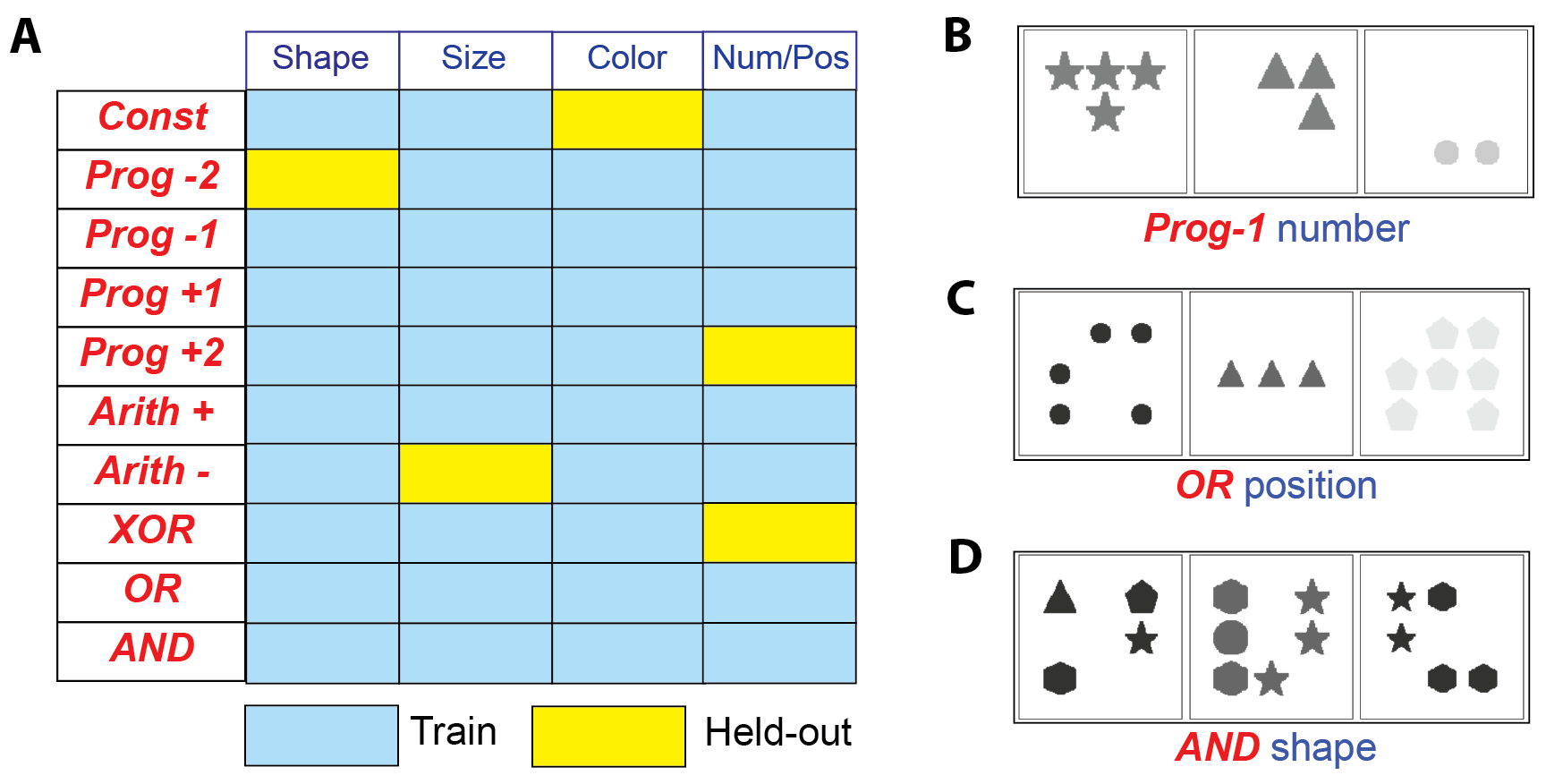
Inspired by the RPM task, the SimplifiedRPM dataset was specifically designed to assess a model’s ability to generalize abstract relations across different object attributes (Fig. 1). Each row in the dataset follows a unique relational rule that determines how an object’s attribute values change across three panels (figure S6A). The dataset consists of relational rules, each derived by applying an abstract relation to a specific object attribute. These abstract relations fall into three categories: progression (constant, progression , progression ), arithmetic (addition, subtraction), and logical (AND, OR, XOR). A detailed description of the abstract relations is provided in Table S1.
Each rule was applied to one of four object attributes: shape, size, shade, or number/position (Fig. S6). Number and position were grouped as a single attribute to avoid ambiguity. For example, a ”constant position” rule inherently fixes the object count, enforcing the constant number rule and conflicting with our requirement that each row in the task follows a unique relational rule. To ensure consistency with prior benchmarks, the dataset adopts the same object definitions and attribute specifications as the PGM dataset (?). Shape is selected from seven geometric forms: circle, triangle, square, pentagon, hexagon, octagon, and star. The objects’ sizes are represented by their bounding boxes in the panel, with heights ranging from to pixels in ten evenly spaced increments. Shade is represented as a grayscale intensity, ranging from (close to white) to (black) in RGB values, with evenly spaced increments. The number attribute specifies the number of objects per panel, ranging from to . Position refers to the spatial arrangement of objects. Each panel has a total size of , and each object occupies a maximum bounding box of . There are nine possible object locations, each defined by its centroid coordinates: . Consequently, each row has dimensions . When presented, the three panels are arranged horizontally.
Dataset generation followed a structured pipeline to ensure consistency and reproducibility. Each row was constructed to enforce a unique rule from our predefined set, eliminating ambiguity. To achieve this, we first sampled attribute values from valid options that conformed to the designated rule. Next, we randomly assigned values to the remaining attributes and resampled if a sampled value inadvertently conformed to an unintended rule. Once attribute values were finalized, they uniquely defined an input row. The corresponding row input was then generated by placing objects with the specified attributes in their designated positions. To maintain dataset balance, we generated 10,000 training rows, 1,000 validation rows, and 1,000 test rows per rule, yielding a total of 48,000 unique rows across all rules (40 rules 1,200 samples). Example rows in the dataset are provided in figure S6B-D.
Neural Network Training
To evaluate a model’s ability to generalize abstract relations to unseen object attributes, we implement a rule-splitting strategy in which a subset of rules is withheld during training. Specifically, we randomly select five rules to be held out, ensuring that each abstract relation appears at most once in this set. The remaining rules are used for model training. After training, the model is evaluated based on its ability to infer the held-out rules. Fig. S6A provides an example of this rule split, with held-out rules highlighted in yellow and training rules in blue.
During training, models are optimized using supervised learning with a cross-entropy loss function. The models are trained on 10,000 examples per rule across training rules. Test error (Fig. 1C) is assessed based on classification accuracy using test examples per rule. These test examples differ from the training examples used during model training.
After training, we evaluate the model’s ability to infer previously unseen, held-out rules. For each pair of the five held-out rules (20 possible rule pairs), we generate 500 SimplifiedRPM trials. Each trial is constructed by randomly sampling two rows from the first rule—one as the sample row and the other as the correct choice. Then, we sample a row from the second rule as the incorrect choice. Finally, we ensure all 500 trials per rule pair are unique.
To evaluate model performance, we compute the Euclidean distance between the sample row and each of the two choice rows. A trial is considered correct if the correct choice row is closer to the sample row than the incorrect one. The model’s generalization error is then quantified as the proportion of incorrect trials averaged across all trials for each of the rule pairs (Fig. 1E).
We trained four architectures: ResNet-50, WReN, ViT, and SCL. ResNet-50 (?) is a convolutional neural network with residual connections. We employed the standard ResNet-50 architecture without modification. WReN (?) explicitly models pairwise relations between objects and has been previously used for RPM tasks. We optimized the hyperparameters of its relation module and fully connected layers. ViT (?) is a transformer-based model that operates on image patches as input tokens and captures global dependencies via self-attention. We split each of the three panels in a row into a grid, resulting in patches per row. We optimized key hyperparameters, including the number of layers, attention heads, and hidden dimensions. Finally, SCL (?) was specifically designed for the RPM task, and we used the original architecture without modifications. Detailed model configurations, including layer-wise specifications and hyperparameter tuning, are provided in Supplementary Text.
Training was conducted using stochastic gradient descent with a learning rate of , momentum of , and weight decay of . To facilitate stable convergence, we applied a learning rate warmup for the first two epochs, followed by a plateau-based scheduler that reduced the learning rate by whenever the validation loss plateaued. Training continued until the classification errors across validation rows for each of the training rules stabilized. The final training durations for each model were: ResNet-50 ( epochs), WReN ( epochs), ViT ( epochs), and SCL ( epochs). All models were trained using a batch size of .
Human Experiment
Twenty-five participants were recruited via Amazon Mechanical Turk (MTurk) to evaluate performance on the SimplifiedRPM dataset. To ensure data reliability, we set strict eligibility criteria, requiring an approval rating above and restricting participation to Masters-qualified workers. All participants provided informed consent, and the study protocol was approved by the Institutional Review Board at Children’s Hospital, Harvard Medical School. Compensation was performance-based, with participants earning more for higher accuracy.
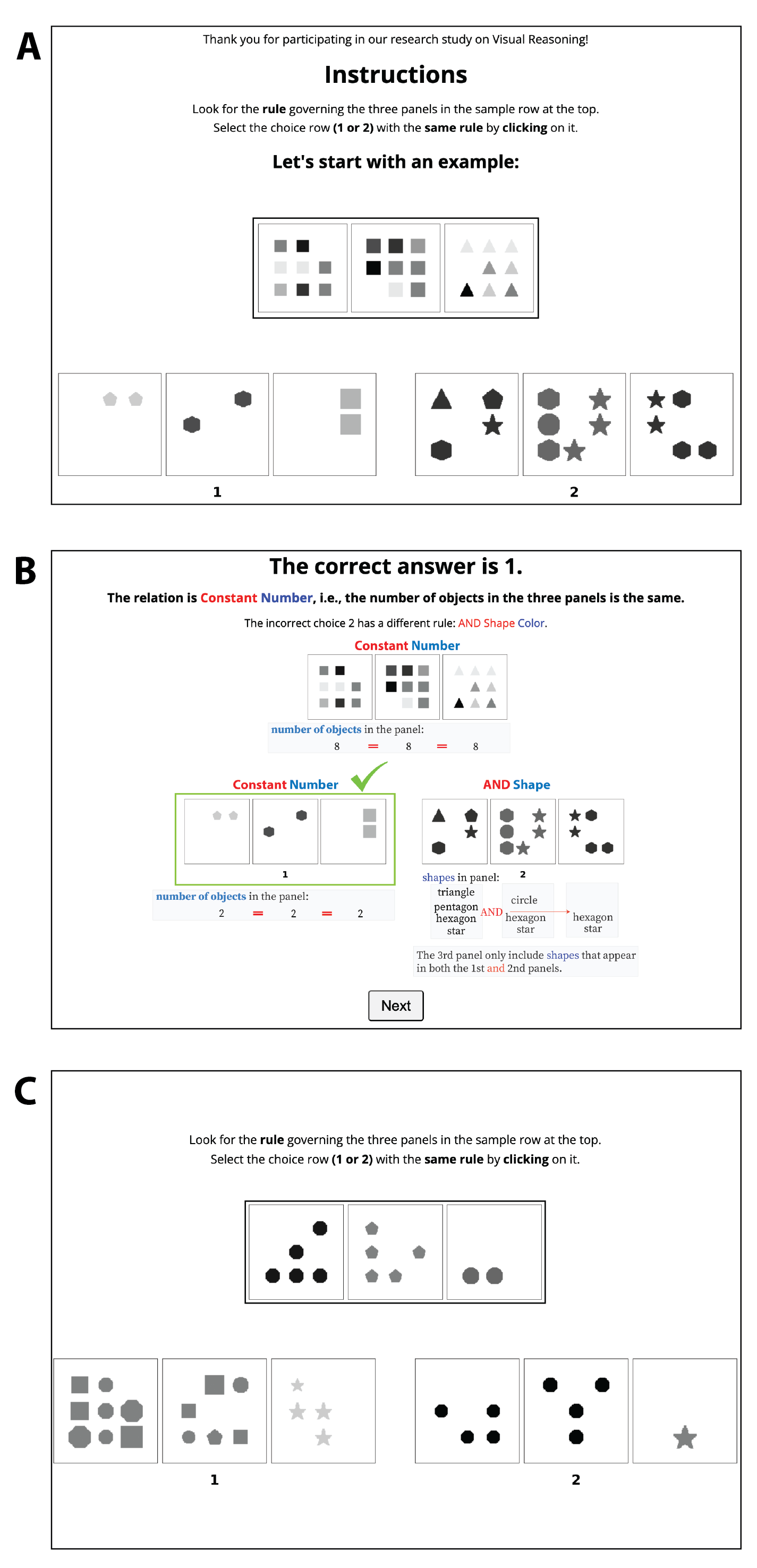
Before the main experiment, participants read written instructions describing the task and completed three practice trials that introduced relational rules different from the rule pairs used in the main experiment. Participants received feedback and explanations of the underlying rules during these practice trials. In the main experiment, each participant completed 60 trials randomly selected from a larger pool of trials ( trials per rule pair), encompassing distinct rule pairs of varying relational complexity (Table S2). Participants were shown images like those in Fig. 1A. The images remained on the screen until the participants made a choice. Participants responded by clicking on one of two choice rows and were allowed unlimited time to provide their answers. No performance feedback was given during the main experiment. Additional information, including illustrative example trials, can be found in figure S7.
Supplementary Text
Model Architecture and Hyperparameter Tuning
We used the standard ResNet-50 architecture described by (?) without any modifications. The architecture comprises residual blocks containing convolutional layers followed by batch normalization and ReLU activation. Specifically, the model begins with an initial convolutional layer, followed by four residual blocks, and concludes with a global average pooling layer and a fully connected layer for classification. To analyze the evolution of layer-wise geometry, we extracted features from the outputs of each residual block (Block 1–4) and the final output of the average pooling layer (avgpool).
The Wild Relation Network (WReN) model captures and integrates pairwise relational information from the three panels in an input row. Each panel is first processed through a shared four-layer convolutional block to generate an individual panel embedding. Then, embeddings from each pair of panels are concatenated and passed through a multi-layer perceptron (MLP). The resulting pairwise features are summed to form an aggregated relational representation, which is further refined through three additional MLP layers. For layer-wise geometric analysis, we extract representations from the convolutional block output (CNN), the aggregated pairwise features (Pairwise), and the three successive MLP layers (MLP1–3).
For hyperparameter tuning of WReN, we performed a grid search over the following parameters: (1) hidden dimension of the pairwise relational module ; (2) number of layers in the pairwise relational module ; (3) hidden dimension of the classification MLP ; and (4) number of layers in the classification MLP . The optimal configuration, minimizing test error on three held-out rule splits, was found to be a pairwise relational module with layers of dimensions and a classification MLP with layers of dimensions.
The Vision Transformer (ViT) architecture comprises multiple layers of multi-headed self-attention (MSA). In our implementation, we utilize a four-layer Transformer model, each containing attention heads and a hidden dimension of . The model processes input row patches, embedding them into token representations with a learnable class token prepended to the sequence. These representations are then sequentially processed through self-attention layers to capture global contextual dependencies. For layer-wise geometric analysis, we extract the outputs from each attention layer (Attn1-4).
For hyperparameter tuning of ViT, we performed a grid search over the following parameters: (1) number of layers ; (2) number of attention heads ; (3) hidden dimension of the self-attention layers . The optimal configuration, determined by minimizing test error, was found to be layers, each with heads and a hidden dimension of .
The Scattering Compositional Learner (SCL) model (?) is a hierarchical architecture designed explicitly for RPM tasks (figure S8). Each input panel is first processed through a shared convolutional block, producing an individual panel embedding. These embeddings are then processed through three 1-D convolutional layers that operate across the three panels. Crucially, the same filter is applied consistently across the panel-wise feature dimensions, ensuring that abstract relations are detected in an attribute-invariant manner. Finally, the output is further refined using two MLP layers. For layer-wise geometric analysis, we extract representations from the convolutional block (CNN), the three 1-D convolutional layers (conv1-3), and the two MLP layers (MLP1–2).
For hyperparameter tuning of SCL, we performed a grid search over the following parameters: (1) the kernel size of the 1-D convolutional layers ; (2) the number of output channels, chosen from for the first layer, for the second layer, and for the final layer; (3) the hidden dimensions of the last two layers of the multi-layer perceptron (MLP) . The optimal configuration, determined by minimizing test error, was found to be a kernel size of , output channel sizes of , and an MLP hidden dimension of .
Prototypical loss and SNR loss
For the SNR loss, we conduct a grid search over batch composition and learning rate. Following the setup used in cross-entropy training, we maintain a total batch size of and explore three batch compositions: ( classes samples per class). Additionally, we test three learning rates: . Model performance is evaluated based on test error across three held-out rule splits, distinct from the used for training. The optimal configuration is with a learning rate of .
The prototypical loss (?) is a distance-based loss function commonly used in few-shot learning. It generates rule prototypes, which act as representative representations for each rule. Like the SNR loss, each input batch consists of rows drawn from different relational rules. For each rule , the rows are randomly split into two disjoint subsets: a support set and a query set . The prototype for rule is computed as the mean representation of its support set:
| (S1) |
where denotes the relational representation of an input row.
The prototypical loss encourages rows in the query set to be closer to their corresponding rule prototype while pushing them away from prototypes of other rules in the batch. It is formulated as:
| (S2) |
To optimize the Prototypical loss, we conducted a grid search over: (1) batch size ( classes samples per class); (2) learning rate , and support set size . Model performance was assessed using test accuracy on three held-out rule splits, distinct from the 15 used for training. The optimal configuration was found to be classes samples per class, with a learning rate of and support set size .



| Relation Type | Relation | Description | Example |
|---|---|---|---|
| Progression | Const | Attribute values are the same across all three panels. | {[1], [1], [1]} |
| Prog -2 | Attribute values decrease incrementally by 2 across the panels. | {[4], [2], [0]} | |
| Prog -1 | Attribute values decrease incrementally by 1 across the panels. | {[2], [1], [0]} | |
| Prog +1 | Attribute values increase incrementally by 1 across the panels. | {[0], [1], [2]} | |
| Prog +2 | Attribute values increase incrementally by 2 across the panels. | {[0], [2], [4]} | |
| Arithmetic | + | Attribute values in the 3rd panel are the sum of the values in the first two panels. | {[0], [1], [1]} |
| - | Attribute values in the 3rd panel are the first panel’s values minus the second panel’s values. | {[1], [1], [0]} | |
| Logical | AND | 3rd panel contains attribute values present in both the first and second panels. | {[0], [0, 1], [0]} |
| OR | 3rd panel contains attribute values present in either the first or second panel. | {[0], [0, 1], [0, 1]} | |
| XOR | 3rd panel contains attribute values present in only one of the first two panels. | {[0], [0, 1], [1]} |
| # | Correct Rule | Incorrect Rule | Human Error | Response Time (sec) |
|---|---|---|---|---|
| 1 | Prog-1 Number | AND Shape | ||
| 2 | Prog+1 Number | Const Number | ||
| 3 | OR Shape | Arith+ Number | ||
| 4 | Prog+2 Number | Const Number | ||
| 5 | Arith- Number | OR Shape | ||
| 6 | XOR Shape | AND Position | ||
| 7 | Prog-2 Number | XOR Position | ||
| 8 | Arith+ Number | OR Position | ||
| 9 | Const Number | Prog+2 Number | ||
| 10 | AND Position | Prog-2 Number | ||
| 11 | AND Shape | XOR Shape | ||
| 12 | OR Position | XOR Position | ||
| 13 | XOR Position | Arith- Number |