Sustainable Greenhouse Management: A Comparative Analysis of Recurrent and Graph Neural Networks

Abstract

The integration of photovoltaic (PV) systems into greenhouses not only optimizes land use but also enhances sustainable agricultural practices by enabling dual benefits of food production and renewable energy generation. However, accurate prediction of internal environmental conditions is crucial to ensure optimal crop growth while maximizing energy production. This study introduces a novel application of Spatio-Temporal Graph Neural Networks (STGNNs) to greenhouse microclimate modeling, comparing their performance with traditional Recurrent Neural Networks (RNNs). While RNNs excel at temporal pattern recognition, they cannot explicitly model the directional relationships between environmental variables. Our STGNN approach addresses this limitation by representing these relationships as directed graphs, enabling the model to capture both spatial dependencies and their directionality. Using high-frequency data collected at 15-minute intervals from a greenhouse in Volos, Greece, we demonstrate that RNNs achieve exceptional accuracy in winter conditions ($R^{2}=0.985$) but show limitations during summer cooling system operation. Though STGNNs currently show lower performance (winter $R^{2}=0.947$), their architecture offers greater potential for integrating additional variables such as PV generation and crop growth indicators.

1 Introduction

Modern agriculture faces increasing pressure to optimize land use while reducing its environmental impact. The integration of photovoltaic (PV) systems into agricultural greenhouses has emerged as a promising solution to these challenges, offering dual benefits of food production and renewable energy generation. However, this integration introduces new complexities in greenhouse management, as PV panels directly influence light distribution, temperature patterns, and overall microclimate dynamics. These Agri-PV systems optimize land use by combining solar energy harvesting with protected crop cultivation, offering potential benefits for both energy and food security. However, the successful implementation of PV-integrated greenhouses requires accurate prediction and control of the internal microclimate to ensure optimal growing conditions while maximizing energy production. While sophisticated physical models incorporating greenhouse thermodynamics, crop physiology, and PV system performance exist, their complexity often limits their practical application in real-time control systems and rapid design optimization. This study, conducted within the framework of the European REGACE project, represents an initial step toward developing a comprehensive digital twin for PV-integrated greenhouses. Rather than relying on complex physical models, this research explores empirical approaches using advanced machine learning techniques to predict greenhouse microclimates. The focus on neural network-based models aims to establish a foundation for a more complete digital twin that will ultimately integrate crop growth dynamics and PV energy production. By comparing traditional Recurrent Neural Networks (RNNs) with directed Spatio-Temporal Graph Neural Networks (STGNNs), this investigation examines whether the explicit modeling of spatial relationships and directional influences can improve prediction accuracy while maintaining computational efficiency.

Effective control and optimization of PV-integrated greenhouse environments presents a fundamental challenge. The success of these hybrid systems relies critically on accurate modeling and prediction of their internal microclimates. Precise prediction of internal parameters such as temperature enables growers to make informed decisions regarding ventilation, heating, cooling, and irrigation systems. Modeling the greenhouse microclimate is a complex task due to the interactions between internal and external environmental factors. External conditions such as ambient temperature, humidity, solar radiation, and wind speed significantly influence the internal climate of a greenhouse. Traditional modeling approaches fail to capture these nonlinear and dynamic relationships, especially when dealing with large datasets collected at high-frequency intervals.

Researchers have developed increasingly sophisticated methods to understand and predict greenhouse behavior, leading to both breakthroughs and new challenges. Greenhouses represent complex thermodynamic systems where the interaction between external environmental conditions and internal microclimate impacts crop growth and energy efficiency. The increasing integration of photovoltaic (PV) technology in greenhouse structures has added new layers of complexity to these systems, requiring more advanced modeling approaches to understand and optimize their performance. These approaches range from detailed physical models to more recent data-driven methods. Dynamic Building Simulation (DBS) has proven to be a robust tool for estimating trends in greenhouse environmental variables and energy demands. Researchers have dedicated efforts to studying structural configurations, ventilation systems, and the implications of evapotranspiration on environmental parameters. Stanciu et al. (2016) investigated the thermal dynamics within polyethylene greenhouses, analyzing orientation effects and ventilation regimes in seasonal extremes while emphasizing evapotranspiration’s role. Similarly, Abdel-Ghany & Kozai (2006) evaluated glass greenhouses focusing on temperature and humidity fluctuations during summer periods, highlighting the impact of evapotranspiration processes. The evolution of greenhouse modeling has seen increasing sophistication in approach and scope. Mobtaker et al. (2019) studied thermal transmittance through different glass roof shapes and orientations, while Singh et al. (2018) advanced this approach by developing comprehensive models integrating natural ventilation and evapotranspiration analysis using Matlab-Simulink. Fitz-Rodríguez et al. (2010) created variable models applicable across different locations, considering structural parameters and integrated heating/cooling systems. Recent innovations in greenhouse sustainability have introduced new modeling challenges. Ouazzani Chahidi et al. (2021) simulated glass-covered greenhouses integrated with photovoltaic panels and geothermal pumps, focusing on internal temperature regulation and energy efficiency. Baglivo et al. (2020) employed TRNSYS software for greenhouse simulation, incorporating plant evapotranspiration, natural ventilation, and temperature control systems. Furthermore, Brækken et al. (2023) used the software IDA ICE for dynamic greenhouse modeling, examining the influence of structural designs and operational systems on yearly temperature, humidity, and energy patterns.

These studies demonstrate the significant advancements made in physical modeling approaches while highlighting their inherent challenges. Physics-based models provide valuable insights into greenhouse dynamics, but they face three critical limitations. First, they require extensive computational resources that make real-time applications challenging. Second, they demand detailed knowledge of system parameters that may not be readily available or may change over time. Third, this complexity is further amplified in PV-integrated greenhouses, where models must simultaneously address energy generation, crop production, and microclimate control.

These limitations have sparked a fundamental shift in greenhouse modeling strategies. Researchers began exploring data-driven approaches that could learn system behavior directly from observations, rather than attempting to model every physical interaction explicitly. This significant change, coupled with advances in computational capabilities and the increasing availability of sensor data, has led to the emergence of artificial intelligence and machine learning approaches as promising alternatives.

The evolution of neural networks in greenhouse modeling spans three decades, following a progression in complexity and capability. Early work by Seginer et al. (1994) and Bussab et al. (2007) demonstrated the potential of basic neural networks for greenhouse modeling. The field advanced through several architectural innovations: Ferreira et al. (2002) and Patil et al. (2008) introduced sophisticated approaches with Radial Basis Function Neural Networks (RBFNNs) and hybrid training methods, while D’Emilio et al. (2012) achieved sensor-level accuracy using Multi-layer Perceptron (MLP) networks with optimized architectures.

A major step forward came with Recurrent Neural Networks (RNNs), particularly their Long Short-Term Memory (LSTM) variants, which transformed temporal modeling in greenhouse environments. RNNs demonstrated superior capabilities in handling time-dependent relationships, starting with Fourati & Chtourou (2007) work. Later studies by Gharghory (2020), and Hongkang et al. (2018) validated RNNs’ effectiveness across various climatic conditions, establishing them as the predominant approach for temporal modeling.

Parallel to RNN developments, researchers explored complementary approaches to address different aspects of greenhouse modeling. MLPs demonstrated high-accuracy predictions, with Petrakis et al. (2022) achieving accuracy ($R^{2}$ values of 0.999) using Levenberg-Marquardt backpropagation. The Nonlinear AutoRegressive model with eXogenous inputs (NARX) emerged as another effective approach, with Manonmani et al. (2018) and Gao et al. (2023) demonstrating its capability in handling the non-linearity of greenhouse systems and adapting to dynamic environmental changes.

Recent advances in computational capabilities have enabled more sophisticated architectures. Salah & Fourati (2021) showed how deeper neural networks improve both modeling and control tasks, while Alaoui et al. (2023) demonstrated that these advanced neural approaches match the accuracy of computational fluid dynamics models with significantly reduced computational cost. This evolution toward more complex architectures aligns with Escamilla-García et al. (2020)’s comprehensive review, which identified the untapped potential of hybrid networks while highlighting the continued dominance of feedforward architectures. The integration of dynamic modeling, neural networks, and heuristic algorithms has emerged as a key trend, as noted in Guo et al. (2020)’s review of recent developments.

Despite these advances in neural network architectures, a fundamental limitation remains: the inability to simultaneously capture both temporal patterns and spatial relationships in an interpretable way. This limitation is particularly problematic for PV-integrated greenhouses, where the complex interactions between environmental variables create a network of interdependencies that traditional neural networks cannot effectively model. The influence of solar radiation on internal temperature varies depending on the PV panel configuration, which in turn affects humidity distribution and crop transpiration rates a web of relationships that requires explicit spatial modeling.

This limitation is critical in PV-integrated greenhouses, where understanding the complex interactions between environmental parameters, crop conditions, and energy generation is essential for optimal control. While RNNs excel at modeling temporal dependencies, they treat each variable as an independent time series, failing to capture the spatial relationships within the greenhouse system.

Spatio-Temporal Graph Neural Networks (STGNNs) offer three key advantages over existing approaches to address this critical gap. First, STGNNs explicitly model directional relationships between variables, capturing how changes in one parameter influence others. Second, they provide simultaneous modeling of both temporal evolution and spatial dependencies, maintaining the temporal modeling capabilities that made RNNs successful while adding spatial awareness (Jain & Medsker (1999), Goodfellow et al. (2016)). Third, they offer an interpretable representation of the greenhouse system as a physical graph structure Yu et al. (2018). By representing environmental variables as nodes and their relationships as edges, STGNNs learn the complex dynamics of the greenhouse microclimate, including crucial directional influences such as how external temperature affects internal humidity, a capability that traditional graph neural networks, with their undirected graph assumptions, lack.

Direct applications of STGNNs in greenhouse environments remain limited. However, related advances in energy and thermodynamic systems (Yu et al. (2018); Sun et al. (2022)) demonstrate potential for integrating new variables such as PV generation data and crop phenological indicators. The graph structure of STGNNs aligns with the concept of digital twins, representing both the physical structure of the greenhouse and the interactions between its components. This representation enables the digital twin to predict system behavior and reveal relationships between environmental variables. The empirical approach using STGNNs complements traditional physical models. A neural network-based digital twin that estimates key parameters and energy flows provides designers and researchers with a tool for rapid initial assessment of PV greenhouse systems. This capability serves in the early stages of development, enabling exploration of different configurations before moving to detailed physical modeling that requires expertise across multiple disciplines, from thermodynamics and fluid dynamics to plant physiology and photovoltaic engineering.

This work presents the first application of STGNNs to PV-integrated greenhouse modeling, building on these insights and introducing two key innovations: (1) explicit modeling of directional environmental interactions specific to greenhouse systems, (2) a hybrid architecture that combines spatial awareness with temporal prediction. This approach differs from previous work by treating the greenhouse as an interconnected system rather than a collection of independent variables. The study validates this approach using data collected from a Mediterranean greenhouse in Volos, Greece a location selected for its representative climate conditions. The analysis examines performance across summer, winter, and autumn periods to capture the range of environmental conditions. The effectiveness of the approach is evaluated through multiple metrics: prediction accuracy (RMSE, MAE), model interpretability (attention weights analysis), and computational efficiency compared to traditional physical models. The implementation uses an STGNN architecture that combines Graph Attention Networks (GATs), selected for their ability to dynamically weight the importance of different environmental relationships based on context. Unlike simpler graph neural networks that treat all connections equally, GATs learn which relationships are most relevant for different prediction tasks and environmental conditions (Vaswani et al. (2017); Veličković et al. (2018); Hochreiter & Schmidhuber (1997)). This hybrid approach enables simultaneous modeling of variable influences across space (through weighted graph edges) and time (through LSTM temporal patterns).

This study establishes a new paradigm for greenhouse modeling that combines prediction accuracy with physical interpretability by evaluating the capabilities of RNNs and directed STGNNs. This approach impacts both research and practical applications, offering greenhouse operators reliable and interpretable tools for climate control while providing researchers with insights into the complex interactions within these systems. The study focuses on temperature prediction as the primary validation metric, with the framework designed to accommodate additional environmental parameters and crop growth indicators in future extensions. The chosen greenhouse configuration represents a typical Mediterranean installation, though adaptations are needed for different climatic zones.

Moreover, This work represents a relevant step in the REGACE project’s broader goal of developing comprehensive digital twin solutions for PV-integrated greenhouses. By establishing the effectiveness of STGNNs for microclimate prediction, it lays the foundation for future integration of crop growth models and PV generation optimization within the same framework.

The paper is structured as follows: Section 2 describes the data used in this study, including data collection methods, preprocessing steps, and the handling of missing values. Section 3 outlines the methodologies employed, offering a brief introduction to deep learning, and detailing the architectures and implementation of the RNN and directed STGNN models. Section 4 presents the analysis and results, comparing the performance of the RNN and directed STGNN models in predicting greenhouse temperature across different seasons. Sections  5  6 discuss the findings, their implications for greenhouse management, and potential directions for future research.

2 Data

The data used in this study originates from a PV greenhouse located in Volos, Greece, for the year 2020, covering from January 9, 2020, to December 21, 2020. The dataset consists of measurements recorded at 15-minute intervals, resulting in 33,446 data points.

The features considered during the analysis are given below. The labels used during the analysis are shown in parentheses:

• External Environmental Factors:

  • External Temperature (OUT_temp): The ambient temperature outside the greenhouse.

  • External Relative Humidity (OUT_RH): The relative humidity of the air outside the greenhouse.

  • Radiation Level (OUT_rad): The amount of solar radiation received.

  • Wind Speed (OUT_wind_speed): The speed of the wind outside the greenhouse.

• Internal Environmental Factors:

  • Greenhouse Temperature (G2_temp): The internal temperature within Greenhouse.

  • Greenhouse Relative Humidity (G2_RH): The internal relative humidity within Greenhouse.

The graphs of the temperature inside and outside the greenhouse for the three periods considered follow:

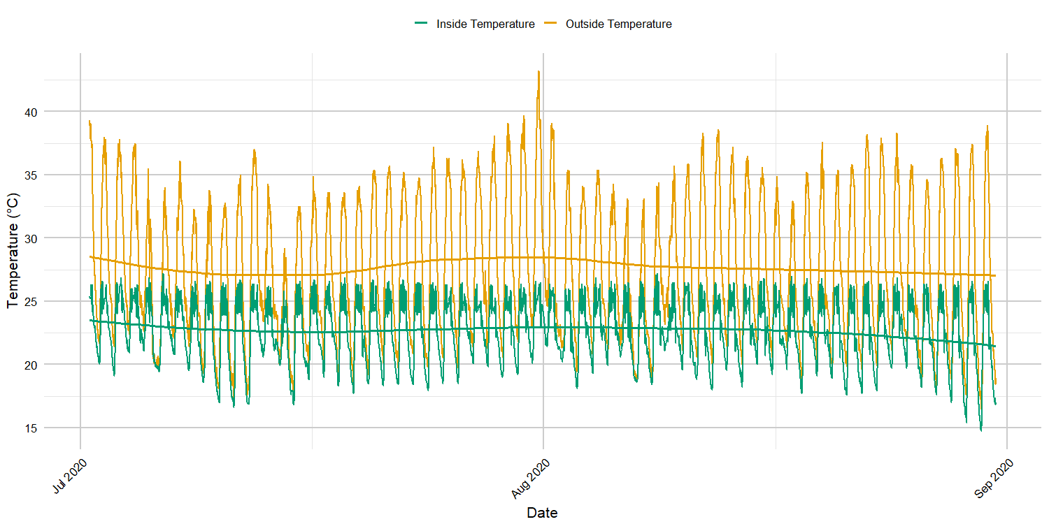
Figure 1: Temperatures inside and outside the greenhouse for the summer period

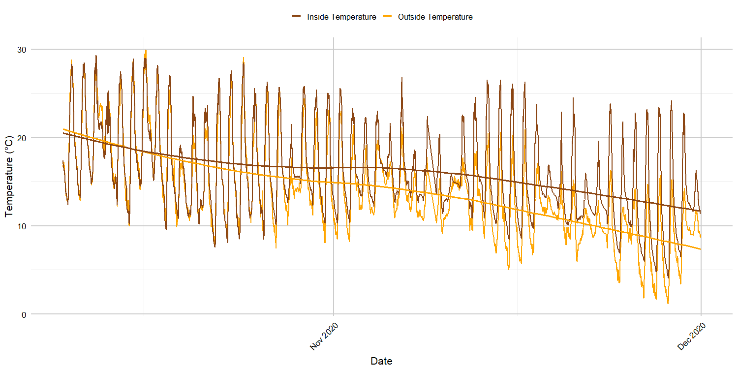
Figure 2: Temperatures inside and outside the greenhouse for the autumn period

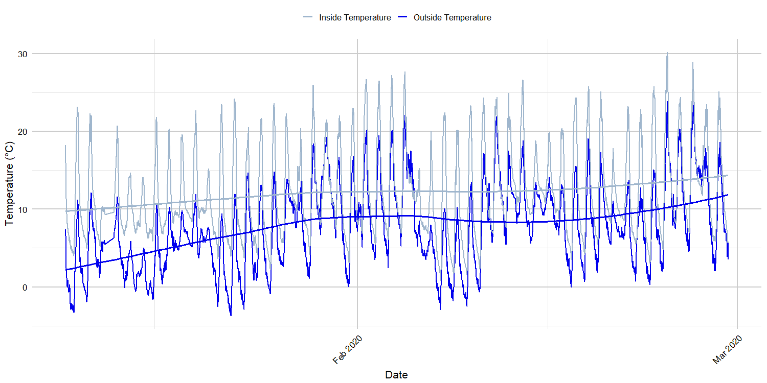
Figure 3: Temperatures inside and outside the greenhouse for the winter period

To capture the complex relationships between these environmental factors, we represent them as nodes in a directed graph, where edges indicate the direction of influence from one variable to another. The graph is presented in Figure 4.

The directed edges in our graph structure represent fundamental physical relationships between environmental variables, based on well-established thermodynamic and atmospheric physics principles. Our choice of edge directions is motivated by the following physical mechanisms:

1. External Relative Humidity Dependencies:

   • Temperature $\rightarrow$ RH: Controls air’s water vapor capacity through the Clausius-Clapeyron relation

   • Wind Speed $\rightarrow$ RH: Affects vapor mixing and transport through turbulent diffusion

   • Solar Radiation $\rightarrow$ RH: Influences evaporation rates and local temperature gradients

2. External Temperature Dependencies:

   • Solar Radiation $\rightarrow$ Temperature: Primary driver through radiative heating

   • Wind Speed $\rightarrow$ Temperature: Modifies heat exchange through forced convection

3. Internal Parameters (Temperature and RH) Dependencies:

   • External Temperature $\rightarrow$ Internal Temperature: Heat transfer through greenhouse envelope

   • External RH $\rightarrow$ Internal RH: Vapor exchange through ventilation and infiltration

   • Solar Radiation → Internal Parameters: Direct heating and greenhouse effect

   • Wind Speed $\rightarrow$ Internal Parameters: Convective heat exchange rate

   • Internal Temperature $\leftrightarrow$ Internal RH: Bidirectional coupling through:

     • Temperature affecting air’s water-holding capacity

     • Humidity influencing evaporative cooling effects

     • Plant transpiration processes

These physical relationships form the basis for the graph structure shown in Figure 4, where each edge represents a direct causal influence between variables. This directed graph approach allows our STGNN model to learn and weight these physical dependencies during the prediction process.

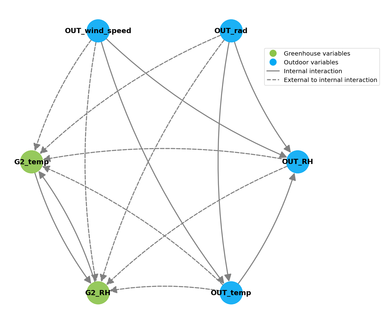
Figure 4: Features’ interaction graph

Moreover, the dataset was divided into three seasons to better investigate the seasonal variations in the greenhouse microclimate and due to the high number of missing data. The dates of the divisions are:

• Summer: From July 1 to August 31,

• Autumn: From October 9 to November 30,

• Winter: From January 9 to February 29.

We used seasonal names for these periods, even though the dates do not perfectly correspond to the year seasons. This discrepancy is due to a significant number of missing values. For the same reason, spring data were excluded from the analysis due to many missing values recorded between April 23 and April 27.

2.1 Data handling

2.1.1 Missing values

Table 1 shows the number of missing values for each variable in each season.

Table 1: Number of missing values for each season

Season	G2_temp	G2_RH	OUT_temp	OUT_RH	OUT_rad	wind_speed
Summer	0	0	0	0	0	0
Winter	68	68	2	2	2	2
Autumn	75	75	75	75	75	75

To address missing data, we employed a combination of linear interpolation and rolling mean techniques. Linear interpolation is effective for high-density time series data, as it estimates missing values by creating a linear equation between the nearest known data points (Malvar et al., 2004; Taewon et al., 2019), as in Equation 1:

$$f(x)=f(x_{o})+\frac{f(x_{1})-f(x_{o})}{x_{1}-x_{o}}(x-x_{o})$$ (1)

where $f$ is the linear interpolation function, $x$ the target value and the subscripts $0$ and $1$ represent respectively the previous and next value from target value. This approach ensured that the imputed values preserved the continuity and trends in the time series without introducing noticeable distortions or flattening in the data sequences. The rolling mean technique was applied in cases where data exhibited more noise or short-term fluctuations, allowing us to smooth these variations while still accounting for missing values.

2.1.2 Normalization

All features were normalized using the min-max method. This scaling brings all values into the range $[0,1]$, bringing all the variables expressed in different units to the same scale and making them comparable (Alaimo & Seri, 2021).

2.1.3 Train-Test Split

To prepare the data for modeling, each seasonal subset of the dataset was divided into training and testing sets while preserving the chronological order. This approach ensured that the integrity of the time series analysis was maintained, as no future information was inadvertently introduced into the training process. The first 80% of observations within each season were allocated to the training set, while the remaining 20% were used for testing. The resulting date ranges for the training and testing sets in each seasonal period are as follows:

• Winter:

  • Training: from 2020-01-09 16:30:00 to 2020-02-19 04:00:00

  • Testing: from 2020-02-19 04:15:00 to 2020-02-29 07:00:00

• Summer:

  • Training: from 2020-07-01 14:30:00 to 2020-08-19 02:45:00

  • Testing: from 2020-08-19 03:00:00 to 2020-08-31 06:00:00

• Autumn:

  • Training: from 2020-10-09 22:00:00 to 2020-11-20 13:00:00

  • Testing: from 2020-11-20 13:15:00 to 2020-11-30 22:45:00

2.2 Stationarity

In order to make statistical inference based on time series data, it is essential to ensure that the underlying data generative process fulfill the stationary property (Kirchgässner et al., 2012). Stationarity means that the statistical properties of the time series, such as mean and variance, remain consistent over time. This consistency is crucial because it ensures that the patterns observed in the past data are applicable to the future. A time series is stationary if it meets two conditions:

1. The mean (average value) of the series is constant over time.

2. The covariance between two points depends only on the time interval between them, not on their specific positions in time.

Stationarity implies that the series fluctuates around a constant level with consistent variation. This property is essential for making reliable inferences and predictions based on the data (Tsay, 2005). To verify that our data met these criteria, we applied the augmented Dickey-Fuller (ADF) test (Cheung & Lai, 1995). The ADF test results indicate that for all variables in all the three considered periods, the null hypothesis of non-stationarity is rejected, confirming that the series are stationary. The results of the ADF test are presented in Tables 4, 5 and 6 in Appendix A.2.1.

3 Methodology

Neural Networks (NNs) are computational models inspired by the human brain’s neural structure. They consist of interconnected nodes (neurons) organized into layers: an input layer, one or more hidden layers, and an output layer. Each connection between neurons has an associated weight that is adjusted during training to minimize prediction error. Deep Neural Networks (DNNs) extend NNs by incorporating multiple hidden layers, enabling the modeling of complex, nonlinear relationships in data. Activation functions such as ReLU, sigmoid, and tanh introduce nonlinearity, while backpropagation adjusts the weights based on the error rate obtained in previous epochs (Nielsen, 2015).

This section outlines the deep learning techniques employed to develop predictive models of greenhouse temperature. We focus on two architectures: Recurrent Neural Networks (RNNs) and directed Spatio-Temporal Graph Neural Networks (STGNNs). We discuss their theoretical foundations, how they are applied in this study, and why they are particularly well-suited for modeling greenhouse microclimates.

3.1 Recurrent neural networks

Recurrent Neural Networks (RNNs) are specialized neural networks designed to process sequential data, making them highly suitable for time-series analysis (Jain & Medsker, 1999). Unlike traditional feedforward neural networks, RNNs have recurrent connections that allow information to persist across time steps, enabling the network to capture temporal dependencies.

An RNN processes sequences one element at a time, maintaining a hidden state that captures information about previous inputs. The hidden state $\bm{h}_{t}$ at time step $t$ is updated based on the current input $\bm{x}_{t}$ and the previous hidden state $\bm{h}_{t-1}$:

$$\bm{h}_{t}=\tanh(\bm{W}_{h}\bm{x}_{t}+\bm{U}_{h}\bm{h}_{t-1}+\bm{b}_{h})$$

The output $\hat{y}_{t}$ at time step $t$ is produced from the hidden state $\bm{h}_{t}$:

$$\hat{y}_{t}=\bm{W}_{y}\bm{h}_{t}+\bm{b}_{y}$$

where $\bm{W}_{h}$, $\bm{U}_{h}$, and $\bm{W}_{y}$ are weight matrices. $\bm{b}_{h}$ and $\bm{b}_{y}$ are bias vectors. $\tanh$ is the hyperbolic tangent activation function introducing nonlinearity. In deeper RNNs, multiple RNN layers are stacked, passing the hidden state from one layer to the next, allowing the model to capture more complex temporal patterns (Nketiah et al., 2023).

RNNs are effective for modeling how current and past environmental conditions influence future states, making them ideal for predicting variables like greenhouse temperature (Rodriguez et al., 1999). A known challenge with RNNs is the vanishing gradient problem, where gradients diminish during backpropagation through time, making it difficult to learn long-term dependencies (Behrang et al., 2010). However, since our data exhibits short-term dependencies, this issue do not impact our study (Dubinin & Effenberger, 2024).

3.1.1 RNN implementation

We begin by preparing the dataset, where each input sequence $\bm{X}^{(i)}$ consists of historical environmental measurements over a period of $T$ time steps. The features include greenhouse temperature and relative humidity, as well as outdoor environmental variables such as temperature, relative humidity, solar radiation, and wind speed. The target value $y^{(i)}$ is the greenhouse temperature at the next time step.

The notation used in our RNN methodology is defined as follows:

• Datasets and Sequences:

  • $\bm{X}^{(i)}\in\mathbb{R}^{T\times F}$: Input sequence for the $i$-th sample, where $T$ is the sequence length and $F$ is the number of features.

  • $y^{(i)}\in\mathbb{R}$: Target value for the $i$-th sample.

  • $N$: Total number of training samples.

• Model Parameters:

  • $E$: Number of training epochs.

  • $B$: Batch size.

  • $\bm{\theta}$: Set of all learnable parameters in the RNN.

• Layers and Functions:

  • $\text{SimpleRNN}(u,\text{return\_seq})$: Simple RNN layer with $u$ units and an option to return sequences.

  • $\text{Dropout}(r)$: Dropout layer with a dropout rate $r$.

  • $\text{Dense}(o)$: Fully connected layer with $o$ output units.

  • $\text{Loss}(\cdot,\cdot)$: Loss function (Mean Squared Error).

  • Optimizer: Optimization algorithm (Adam optimizer).

The RNN model is constructed with two Simple RNN layers, each containing 50 units. The first RNN layer is configured to return sequences (return_sequences=True), allowing the subsequent layer to receive the entire sequence output. Dropout layers with a rate of 0.2 are interleaved between the RNN layers to prevent overfitting by randomly setting a fraction of input units to zero during training. A Dense layer with one unit at the end of the network outputs the predicted temperature.

The model is compiled using the Adam optimizer (Kingma & Ba, 2014), which adapts the learning rate during training for efficient convergence. The loss function is set to Mean Squared Error (MSE), suitable for regression tasks.

Training proceeds for $E$ epochs, where in each epoch, the model is trained on the entire training dataset using batches of size $B$. Optionally, a portion of the training data is set aside for validation to monitor the model’s performance on unseen data during training.

After training, the model is evaluated on the test dataset to assess its predictive performance. Evaluation metrics such as MSE, Root Mean Squared Error (RMSE), and the coefficient of determination ($R^{2}$) are computed to quantify the accuracy of the model’s predictions.

The training algorithm is summarized as follows:

Algorithm 1 Recurrent Neural Network (RNN) Training Algorithm

1:Training sequences $\{(X^{(i)},y^{(i)})\}_{i=1}^{N}$, sequence length $T$, batch size $B$, number of epochs $E$

2:Define model architecture:

3: Layer 1: Simple RNN with 50 units, input shape $(T,F)$, return sequences True

4: Layer 2: Dropout layer with rate $0.2$

5: Layer 3: Simple RNN with 50 units

6: Layer 4: Dropout layer with rate $0.2$

7: Layer 5: Dense layer with 1 unit (output)

8:Compile model with optimizer Adam and loss Mean Squared Error

9:for epoch $=1$ to $E$ do

10:  Train the model on training data with batch size $B$

11:  Optionally validate the model on validation data

12:end for

13:Evaluate the model on test data

14:Compute evaluation metrics (MSE, RMSE, $R^{2}$)

3.2 Spatio-Temporal Graph Neural Networks

To model the spatio-temporal dynamics of the greenhouse microclimate, we employ directed STGNN. This approach integrates Graph Attention Networks (GATs) for spatial feature extraction (Veličković et al., 2018) and Long Short-Term Memory (LSTM) networks (Hochreiter & Schmidhuber, 1997) for temporal sequence modeling. Unlike traditional RNN-based models, which focus primarily on temporal sequences, STGNNs leverage Graph Neural Networks (GNNs) to incorporate topological and relational information among variables. This is well-aligned with recent advances in GNNs for time series (Jin et al., 2024). By representing each environmental variable, such as internal temperature, humidity, and external factors like solar radiation and wind speed, as a node in a directed graph, we capture how changes in one variable may propagate to others through directional edges. Figure 4 illustrates this architecture. Each node corresponds to an environmental variable, while edges encode the direction of influence. At each time step $t$, node features $\bm{X}_{t}$ are extracted from the input sequence $\bm{X}^{(i)}$. To prevent data leakage, the feature of the target node (greenhouse temperature) at the current time step is masked (set to zero) before model input. The GAT layers learn to weigh the importance of edges and neighboring nodes, revealing spatial dependencies, while the LSTM layers capture long-term temporal patterns.

3.2.1 Graph Attention Networks and Directed Graphs

The Graph Attention Network (GAT) layer (Veličković et al., 2018) is employed to handle the directed graph and assign different weights to incoming edges through an attention mechanism. This mechanism allows each node to weigh the importance of its neighbors’ features when updating its own representation.

For each node $i$ and its incoming neighbor $j$, the attention coefficient $\alpha_{ij}$ is computed to determine the importance of node $j$’s features to node $i$:

$$e_{ij}=\text{LeakyReLU}\left(\bm{a}^{\top}\left[\bm{W}\bm{x}_{i}\,\|\,\bm{W}\bm{x}_{j}\right]\right)$$

$$\alpha_{ij}=\frac{\exp(e_{ij})}{\sum_{k\in\mathcal{N}_{i}}\exp(e_{ik})}$$

where:

• $\bm{x}_{i}$ and $\bm{x}_{j}$ are the feature vectors of nodes $i$ and $j$, respectively.

• $\bm{W}$ is a learnable weight matrix.

• $\bm{a}$ is a learnable weight vector (attention mechanism).

• $[\cdot\,\|\,\cdot]$ denotes the concatenation of two vectors.

• LeakyReLU is the activation function introducing nonlinearity.

• $\mathcal{N}_{i}$ is the set of neighboring nodes sending messages to node $i$.

• $e_{ij}$ is the unnormalized attention score.

• $\alpha_{ij}$ is the normalized attention coefficient, representing the weight assigned to node $j$’s features by node $i$.

The LeakyReLU function, characterized by a small positive slope in its negative part, prevents zero gradients and ensures a more robust learning process, especially important in the attention mechanism where gradient flow is crucial for dynamic weight adjustments.

Node Feature Update:

The updated feature vector $\bm{h}_{i}$ for node $i$ is computed by aggregating the transformed features of its neighbors, weighted by the attention coefficients:

$$\bm{h}_{i}=\sigma\left(\sum_{j\in\mathcal{N}_{i}}\alpha_{ij}\bm{W}\bm{x}_{j}\right)$$

where $\sigma$ is an activation function, such as ReLU.

By using the GAT layer, which inherently supports directed graphs, we effectively model the directionality of interactions among environmental variables. The attention mechanism allows the model to assign different weights to incoming edges based on their importance, capturing the dependence relationships in the data.

3.2.2 Long Short-Term Memory (LSTM) Networks

Long Short-Term Memory (LSTM) networks (Hochreiter & Schmidhuber, 1997) are a specialized type of RNN architecture designed to better capture and retain long-term dependencies in sequential data. Unlike traditional RNN units, which can suffer from the vanishing gradient problem, LSTM cells incorporate gating mechanisms, namely the input, forget, and output gates, allowing the network to selectively add or remove information from its internal cell state. This structure enables the LSTM to preserve context over many time steps, making it well-suited for complex temporal sequences where relevant patterns may span extended intervals. In the directed STGNN model, the LSTM layer processes the sequence of GAT outputs $\{\bm{H}t\}_{t=1}^{T}$ to extract temporal features that complement the spatial dependencies learned by the GAT layer.

3.2.3 Directed STGNN model implementation

The notation used in our STGNN methodology is defined as follows:

• Datasets and Sequences:

  • $\bm{X}^{(i)}\in\mathbb{R}^{T\times N_{n}\times F}$: Input sequence for the $i$-th sample, where $T$ is the sequence length, $N_{n}$ is the number of nodes, and $F$ is the feature size per node (here, $F=1$).

  • $y^{(i)}\in\mathbb{R}$: Target value for the $i$-th sample.

  • $N$: Total number of training samples.

• Graph Components:

  • $E$: Edge index representing directed connections between nodes in the graph.

  • $N_{n}$: Number of nodes in the graph.

• Model Parameters:

  • $E_{p}$: Number of training epochs.

  • $B$: Batch size.

  • $H$: Hidden size of the GAT layer.

  • $H^{\prime}$: Hidden size of the LSTM layer.

  • $K$: Number of attention heads in the GAT layer.

  • $\bm{\theta}$: Set of all learnable parameters in the STGNN.

• Layers and Functions:

  • $\text{GAT}(F,H,K)$: GAT layer with input feature size $F$, output size $H$ per head, and $K$ attention heads.

  • $\text{LSTM}(H\times K\times N_{n},H^{\prime})$: LSTM layer with input size $H\times K\times N_{n}$ and hidden size $H^{\prime}$.

  • $\text{Dropout}(r)$: Dropout layer with a dropout rate $r$.

  • $\text{Dense}(o)$: Fully connected layer with $o$ output units.

  • $\text{Loss}(\cdot,\cdot)$: Loss function (Mean Squared Error).

  • Optimizer: Optimization algorithm (Adam optimizer).

Layer 1 (GAT Layer) processes node features $\bm{X}_{t}$ at each time step $t$ using the graph structure defined by $E$. It aggregates information from neighboring nodes based on attention coefficients to capture spatial dependencies. Layer 2 (LSTM Layer) processes the sequence of GAT outputs $\{\bm{H}_{t}\}_{t=1}^{T}$ to capture temporal dependencies over the sequence length $T$. Layer 3 (Dropout Layer) is applied with a rate of 0.2 to mitigate overfitting. Layer 4 (Dense Output Layer) produces the predicted greenhouse temperature $\hat{y}$.

To avoid data leakage, the feature of the target node (greenhouse temperature) at the current time step is set to zero during input preparation. The model is compiled using the Adam optimizer (Kingma & Ba, 2014) and the Mean Squared Error (MSE) loss function. It is trained over $E_{p}$ epochs using batches of size $B$. During training, gradients are computed through backpropagation, and model parameters $\bm{\theta}$ are updated accordingly.

After training, the model is evaluated on the test dataset. Evaluation metrics such as MSE, RMSE, and $R^{2}$ score are calculated to assess the model’s performance.

The training algorithm is summarized as follows:

Algorithm 2 Directed STGNN Training Algorithm

1:Training sequences $\{(\bm{X}^{(i)},y^{(i)})\}_{i=1}^{N}$, edge index $E$, sequence length $T$, batch size $B$, number of epochs $E_{p}$, number of nodes $N_{n}$

2:Initialize model parameters $\bm{\theta}$

3:Define model architecture:

4: Layer 1: $\text{GAT}(F,H,K)$

5: Layer 2: $\text{LSTM}(H\times K\times N_{n},H^{\prime})$

6: Layer 3: $\text{Dropout}(0.2)$

7: Layer 4: $\text{Dense}(1)$ (output layer)

8:for epoch $=1$ to $E_{p}$ do

9:  for each batch $\{(\bm{X}_{\text{batch}},y_{\text{batch}})\}$ do

10:   Forward pass:

11:   for time step $t=1$ to $T$ do

12:     Extract node features $\bm{X}_{t}$ from $\bm{X}_{\text{batch}}$ at time $t$

13:     Prevent data leakage: Set target node feature $\bm{x}_{v}\leftarrow 0$

14:     Apply GAT layer: $\bm{H}_{t}\leftarrow\text{GAT}(\bm{X}_{t},E)$

15:   end for

16:   Stack $\bm{H}_{t}$ over time to form $\bm{H}_{\text{seq}}$

17:   Apply LSTM layer: $\bm{H}_{\text{lstm}}\leftarrow\text{LSTM}(\bm{H}_{\text{seq}})$

18:   Apply Dropout: $\bm{H}_{\text{drop}}\leftarrow\text{Dropout}(\bm{H}_{\text{lstm}})$

19:   Compute output: $\hat{y}\leftarrow\text{Dense}(\bm{H}_{\text{drop}})$

20:   Compute loss: $L\leftarrow\text{Loss}(y_{\text{batch}},\hat{y})$

21:   Backward pass: Compute gradients $\nabla_{\bm{\theta}}L$

22:   Update parameters: $\bm{\theta}\leftarrow\bm{\theta}-\eta\nabla_{\bm{\theta}}L$

23:  end for

24:  Optionally validate the model on validation data

25:end for

26:Evaluate the model on test data

27:Compute evaluation metrics (MSE, RMSE, $R^{2}$)

4 Analysis and results

This section presents the results obtained from applying the RNN and directed STGNN models to the greenhouse temperature prediction task. Both models were trained and tested using a sequence length of $T=96$ time steps, corresponding to a full 24-hour cycle of observations recorded at 15-minute intervals. This setup allowed the models to capture daily patterns and short-term dependencies effectively.

In addition, both models were trained for 32 epochs with a batch size of 96, aligning with practices in comparable studies (Belhaj Salah & Fourati, 2021; Dae-Hyun et al., 2020). Furthermore, 10% of the training set in each seasonal period was used as a validation set to monitor the models’ performance during training. This approach prevented overfitting, evidenced by the validation loss never surpassing the training loss throughout the process.

To facilitate direct comparisons between the RNN and STGNN models, the same evaluation metrics were employed. Mean Squared Error (MSE) and Root Mean Squared Error (RMSE) measured the prediction error magnitude, while the coefficient $R^{2}$ assessed the proportion of variance in greenhouse temperature explained by the model’s predictions.

4.1 Recurrent neural networks application

Table 2 summarizes the test set results obtained by the RNN model for the three considered seasonal periods.

Table 2: RNN test performance across different seasons

Season	MSE	RMSE	$\bm{R^{2}}$
Summer	0.0032	0.056	0.937
Winter	0.0005	0.022	0.985
Autumn	0.0007	0.026	0.983

The RNN demonstrates strong predictive capabilities, achieving high $R^{2}$ values across all seasons. Its performance is particularly impressive in winter, where $R^{2}\approx 0.985$ indicates that the model captures nearly all the variance in greenhouse temperature. This result depends by several factors related to greenhouse operation during the cold season. First, despite winter typically exhibiting large external temperature fluctuations, the greenhouse’s effectively maintains stable internal conditions, making the system’s behavior more predictable. Second, the reduced solar radiation intensity in winter means the greenhouse is less subject to sudden heat gains that could perturb the internal environment. Third, the thermal screen’s regular nighttime deployment (activated whenever the outside temperature is 2°C lower than the heating setpoint) creates a more controlled environment with reduced thermal exchanges. These factors combine to create a more deterministic system behavior that the RNN can effectively learn and predict, despite the external environment’s inherent variability.

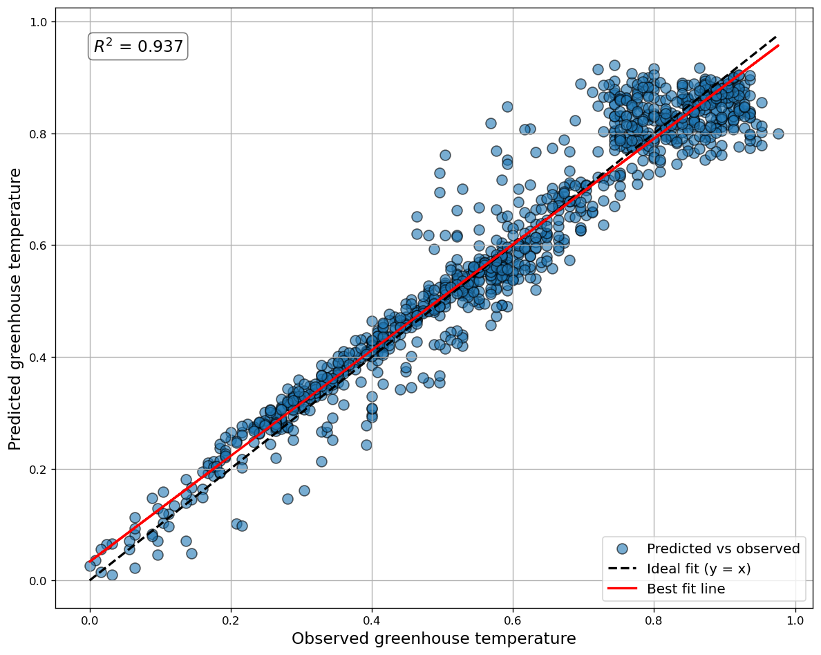
Figure 9: Scatter plot of the observed vs. predicted greenhouse temperature for the summer period using the RNN model.

In contrast, while the summer period still exhibits a high $R^{2}$ of about $0.937$, the prediction errors (MSE and RMSE) are relatively higher, with distinct patterns visible in the model’s performance. As shown in Figure 9 the model’s predictions deviate significantly from observations at higher temperatures, producing a characteristic box-shaped pattern in the scatter plot. This behavior directly results from the greenhouse’s cooling system activation, which triggers when internal temperature reaches a threshold of 25°C. Since our empirical model does not explicitly account for this control system, it fails to capture the sudden temperature regulation that occurs above this threshold. However, examining the lower portion of the scatter plot (below normalized temperature values of 0.6), where the cooling system remains inactive, reveals that the model maintains excellent predictive accuracy. This dichotomy in performance clearly demonstrates how the absence of cooling system dynamics in our model impacts its predictive capabilities, particularly during periods of peak thermal stress when temperature control mechanisms are most active.. Autumn performance falls between these two cases, with $R^{2}\approx 0.983$, indicating strong predictive accuracy albeit slightly less than that seen in winter.

Figure 5 provides a scatter plot comparing observed and predicted greenhouse temperatures during the winter period. Points closely aligned along the 1:1 line signify accurate predictions. Figure 6 shows the time series of actual versus predicted values, illustrating how well the RNN’s predictions track the observed temperatures over time.

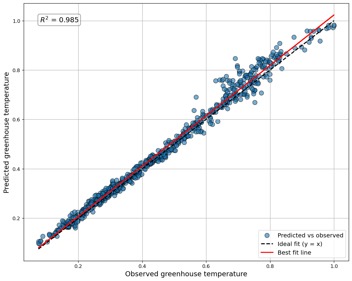
Figure 5: Scatter plot of the observed vs. predicted greenhouse temperature for the winter period using the RNN model.

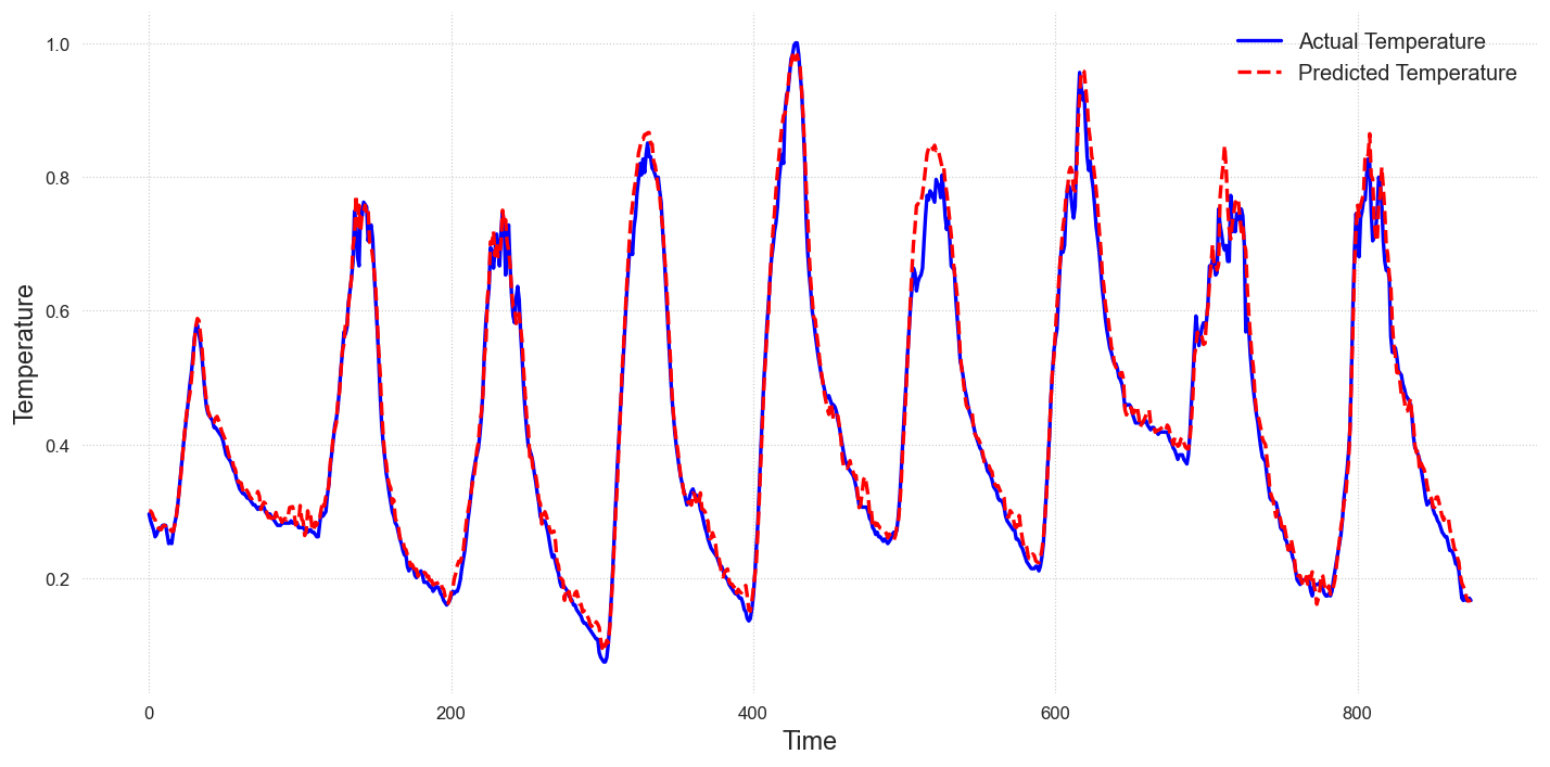
Figure 6: Time series of the observed and predicted greenhouse temperature for the winter period using the RNN model.

Similar plots for summer and autumn are included in Appendix A.1.1. These additional figures reveal analogous tendencies: the model accurately tracks observed temperatures, especially in winter, where conditions appear more stable, allowing the RNN to predict internal temperature with remarkable confidence.

While the RNN achieves robust performance in all three periods, the differences across seasons reveal important insights about greenhouse control systems and model limitations. The near-ideal predictions in winter reflect the greenhouse’s effective temperature stabilization, creating a more predictable environment despite external variability. Autumn shows similar high performance, as temperatures rarely reach extremes requiring intensive control interventions. However, summer predictions show a clear dichotomy: excellent accuracy below the cooling threshold temperature, but significant deviations when the cooling system activates at 25°C. This pattern demonstrates that our empirical model’s performance is strongly tied to the greenhouse’s control regime rather than external conditions alone, performing best when passive thermal regulation dominates and struggling when active cooling interventions occur.

4.2 Spatio-Temporal Graph Neural Network application

Table 3 presents the directed STGNN test set results for the three seasonal periods, using the same evaluation metrics as applied to the RNN model. As before, the sequence length, training epochs, batch size, and validation strategy remain consistent.

Table 3: STGNN test performance across different seasons

Season	MSE	RMSE	$\bm{R^{2}}$
Summer	0.0061	0.078	0.887
Winter	0.0023	0.048	0.947
Autumn	0.0034	0.058	0.904

While the STGNN model still achieves relatively high $R^{2}$ values, its overall performance is lower than that of the RNN. In winter, the STGNN attains an $R^{2}$ of approximately 0.947, which, although strong, falls short of the near-perfect predictions obtained by the RNN. Similarly, in summer and autumn, the STGNN yields lower $R^{2}$ scores and higher MSE and RMSE values than the RNN, indicating that incorporating spatial dependencies and directionality did not enhance predictive accuracy in this particular setting.

Figure 7 provides a scatter plot of observed versus predicted temperatures for the winter period, and Figure 8 shows the corresponding time series comparison. These visualizations confirm that, while the STGNN’s predictions track the overall trends, the model does not reach the same level of precision demonstrated by the RNN.

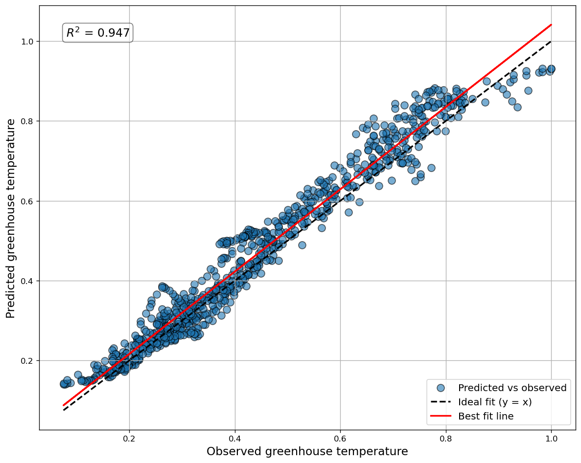
Figure 7: Scatter plot of observed vs. predicted greenhouse temperature for the winter period using the STGNN model.

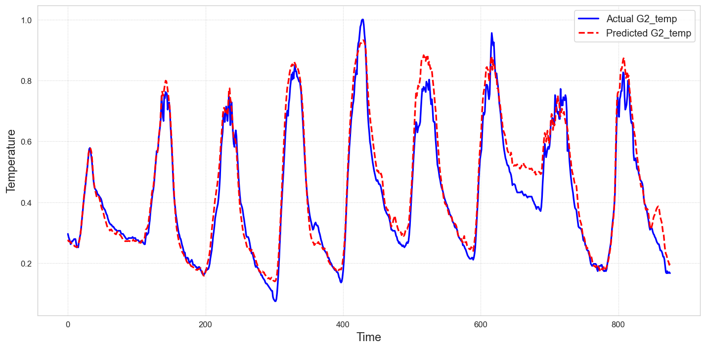
Figure 8: Time series of observed and predicted greenhouse temperature for the winter period using the STGNN model.

Plots for summer and autumn are included in Appendix A.1.2. They similarly show that the STGNN model, despite considering spatial relationships and directed interactions, does not outperform the simpler temporal approach employed by the RNN. This outcome suggests that, for the given data and conditions, capturing complex spatial-temporal dependencies does not necessarily translate into improved predictive accuracy.

5 Discussion

The comparative evaluation of RNN and directed STGNN models for greenhouse temperature prediction provides insights into how each model leverages available information and handles environmental complexity. The strong performance of the RNN, particularly during the winter period suggests that temporal patterns alone can effectively capture many of the dependencies underlying the greenhouse microclimate. Under these circumstances, long-term stationarity and moderate seasonal variations allow historical sequences of internal and external factors to sufficiently inform future conditions. As a result, the RNN consistently achieves near-perfect predictions in such stable regimes.

However, as conditions grow more complex, the advantages of a temporal-only model appear less pronounced. In summer, for example, the accuracy of the RNN decreases, indicating the challenges posed by more dynamic and rapidly fluctuating environmental factors. Abrupt changes in solar radiation, the intermittent operation of cooling systems, or sudden shifts in external temperature highlight a broader limitation: the RNN’s inability to explicitly model the spatial and directional interactions among variables. While it excels in extracting temporal dependencies, it cannot directly encode the influence structure that might clarify why certain variables cause distinct, localized changes or how perturbations propagate from one factor to another.

In principle, the STGNN architecture is designed to address this very limitation. By representing each variable as a node in a directed graph and capturing the directionality of interactions, the STGNN should be well-suited to handle scenarios where spatial relationships and directional effects matter. The GAT component of the STGNN aims to highlight influential nodes and edges, while the LSTM component extracts temporal dependencies. Together, this framework has the potential to disentangle complex spatio-temporal patterns that a purely temporal model may overlook.

Yet, in our experiments, the STGNN did not outperform the RNN. This outcome can be attributed to several factors. First, the set of input variables, though representative of basic external and internal greenhouse conditions, may not be rich enough to fully leverage the STGNN’s spatial modeling capabilities. For instance, without additional features that intensify spatial heterogeneity (e.g., PV generation data influencing localized temperature gradients, or crop growth indicators that reflect biological processes tied to specific sections of the greenhouse), the STGNN may not find compelling reasons to depart from solutions similar to those of a temporal-only model. In other words, if the underlying system appears nearly homogeneous from a spatial perspective, or if directional edges do not provide sufficiently distinct pathways of influence, the added complexity of the STGNN architecture may not yield tangible benefits.

Second, the STGNN’s performance depends on accurately learning graph structures and attention patterns that differentiate the importance of certain nodes and edges. If the graph connections are not strongly differentiated, the GAT may not produce markedly different node embeddings, diminishing the model’s advantage. The LSTM layer, while capable of capturing temporal information, cannot compensate if the spatial relationships remain underexploited.

These observations guide the interpretation of our results. The theoretical superiority of STGNN in handling complex and directed spatio-temporal dependencies is not dismissed by the current findings. Instead, the experiments suggest that to unlock the STGNN’s full potential, the modeling scenario must present more pronounced spatial variations, clearer directional influences, or a richer set of variables that intensify these spatial-temporal complexities. Under such enriched conditions, the STGNN may provide insights and accuracies that temporal-only models cannot match.

6 Conclusions and future developments

This study examined the performance of Recurrent Neural Networks (RNNs) and directed Spatio-Temporal Graph Neural Networks (STGNNs) in predicting greenhouse temperature under different seasonal conditions. Despite the STGNN’s conceptual ability to model spatial and directional relationships, the RNN model yielded higher predictive accuracy given the current set of input variables and operating conditions. The strong performance of the RNN, particularly during the winter period, illustrates that purely temporal modeling can effectively capture short-term dependencies.

The implications of this research extend far beyond technical model comparisons, touching on critical aspects of sustainable agriculture and efficient land use. Predicting greenhouse microclimate accurately is a crucial first step toward integrating photovoltaic (PV) systems into greenhouses. This integration promises to optimize land use by combining energy production with food cultivation, thereby enhancing sustainable agricultural practices. It is instrumental in promoting sustainable land management practices that are vital in addressing global environmental challenges, such as resource efficiency and climate change mitigation.

Looking ahead, a more diverse set of input variables may enhance the potential benefits of incorporating spatial and directional information. Despite the STGNN’s current performance not surpassing the RNN in this specific scenario, its architectural advantages position it as a promising framework for future greenhouse modeling challenges. As we move toward integrating photovoltaic systems, the STGNN’s ability to handle directed relationships will become crucial for modeling how PV panels affect local shading patterns, temperature gradients, and energy flows. The graph structure naturally accommodates the addition of new nodes representing PV generation parameters, inverter efficiency, and panel temperature, along with their complex interactions with the greenhouse environment. Similarly, when incorporating crop models, the STGNN can represent different plant varieties as separate nodes, each with unique growth parameters and responses to environmental conditions, enabling simulation of mixed-crop scenarios within the same greenhouse. This extensibility last to potential future additions such as energy storage systems, artificial lighting, or multiple greenhouse compartments with distinct microclimates. Furthermore, the attention mechanism in GAT layers could prove valuable in identifying which relationships become more or less important under different operating conditions or seasonal changes, providing insights that could inform greenhouse design and control strategies. This scalability and interpretability make the STGNN framework particularly valuable for developing comprehensive digital twins of increasingly complex agricultural systems, even if simpler models may suffice for basic temperature prediction tasks.

Such tests could confirm whether additional complexity and diversity in data naturally lead to scenarios where spatial-temporal modeling offers clear advantages, ultimately guiding the development of more robust and universally applicable predictive solutions for controlled-environment agriculture.

This study represents an initial step in the broader REGACE project’s vision of developing comprehensive digital twins for PV-integrated greenhouses. While our current models focus on temperature prediction, they lay the groundwork for REGACE’s more ambitious goals. The project aims to create an integrated modeling framework that combines greenhouse microclimate prediction with PV system performance and crop growth dynamics. Future work within REGACE will focus on expanding these models to incorporate PV panel characteristics, testing different panel configurations and their impact on both energy generation and crop growth. Additionally, the project will explore how these empirical models can complement detailed physical simulations, potentially offering rapid preliminary assessments for greenhouse design optimization. By developing these tools within the REGACE framework, we aim to support the widespread adoption of agrivoltaic greenhouse systems while ensuring optimal conditions for both energy generation and crop production.

7 Acknowledgment

This research was carried out within the framework of the European REGACE project, funded by the European Union’s Horizon Europe Research and Innovation Programme under Grant Agreement No. 101096056.

Appendix A Supplementary Information

A.1 Figures

A.1.1 RNN results figures

The graphs of the RNN results for the summer and autumn periods follow.

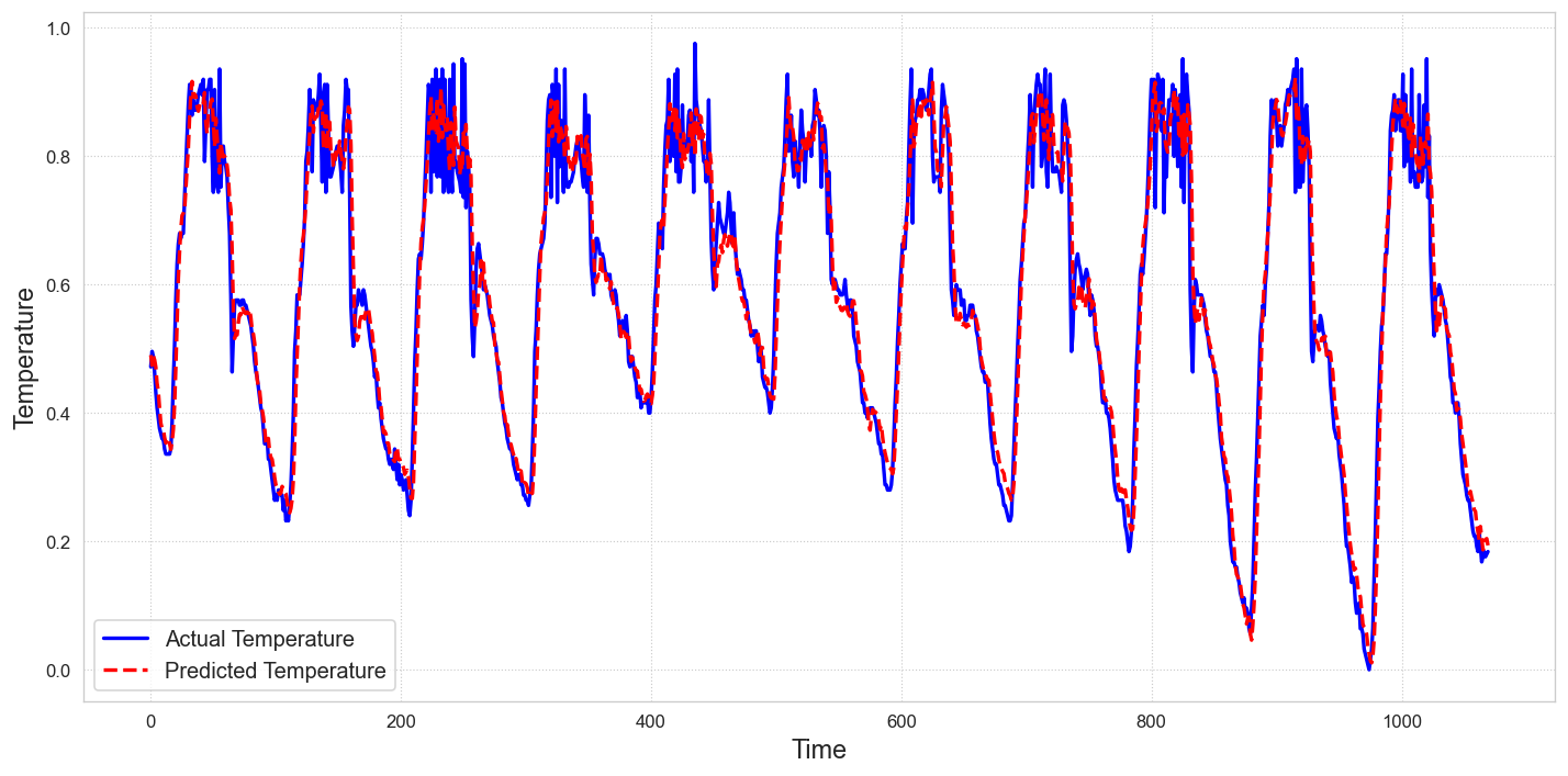
Figure 10: Time series of the observed and predicted greenhouse temperature for the summer period using the RNN model.

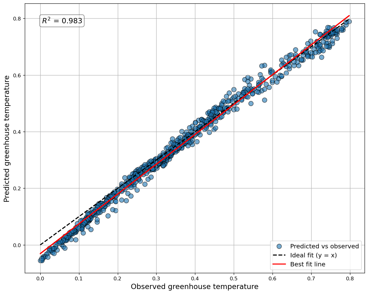
Figure 11: Scatter plot of the observed vs. predicted greenhouse temperature for the autumn period using the RNN model.

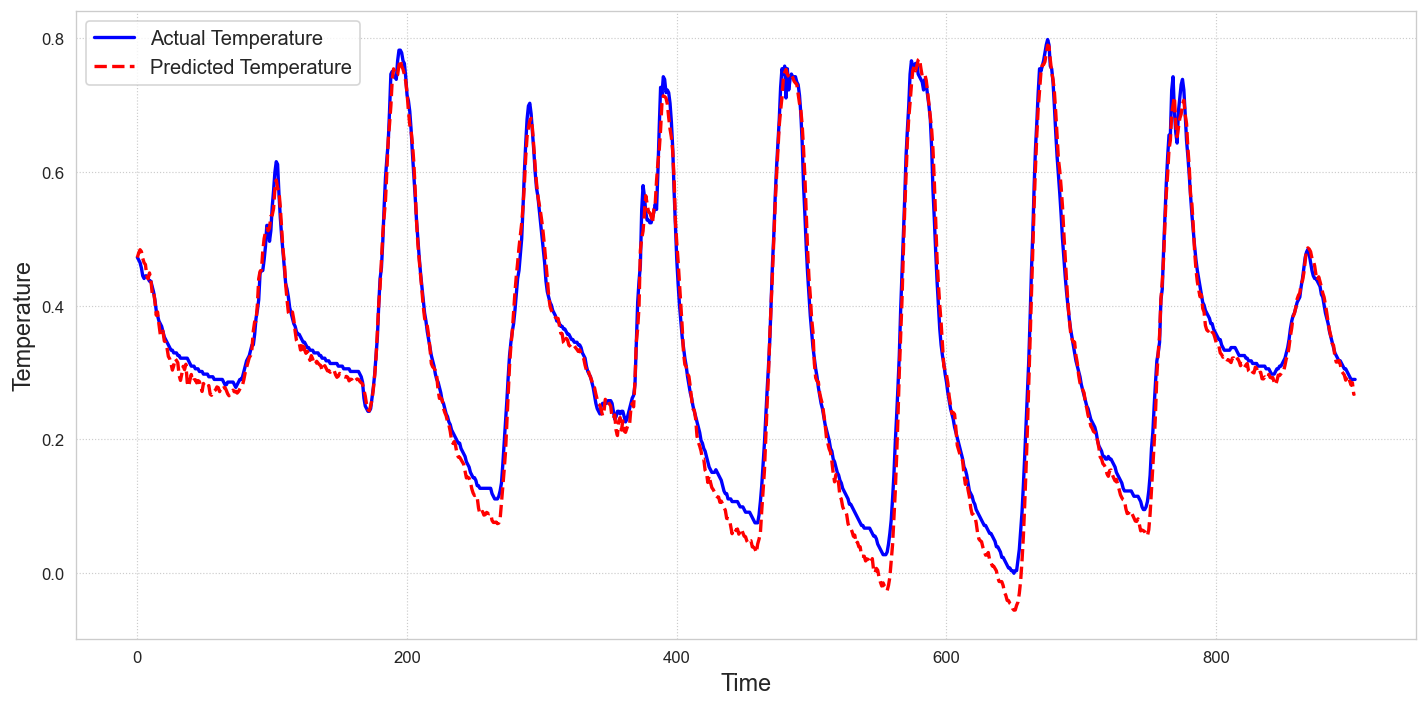
Figure 12: Time series of the observed and predicted greenhouse temperature for the autumn period using the RNN model.

A.1.2 STGNN temperature figures

The graphs of the directed STGNN results for the summer and autumn periods follow.

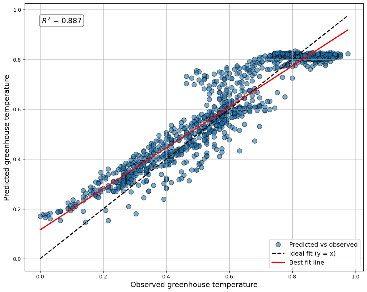
Figure 13: Scatter plot of the observed vs. predicted greenhouse temperature for the summer period using the STGNN model.

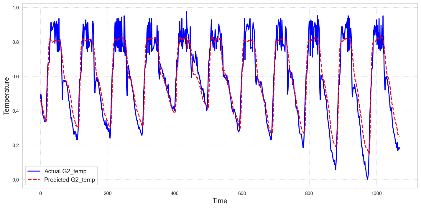
Figure 14: Time series of the observed and predicted greenhouse temperature for the summer period using the STGNN model.

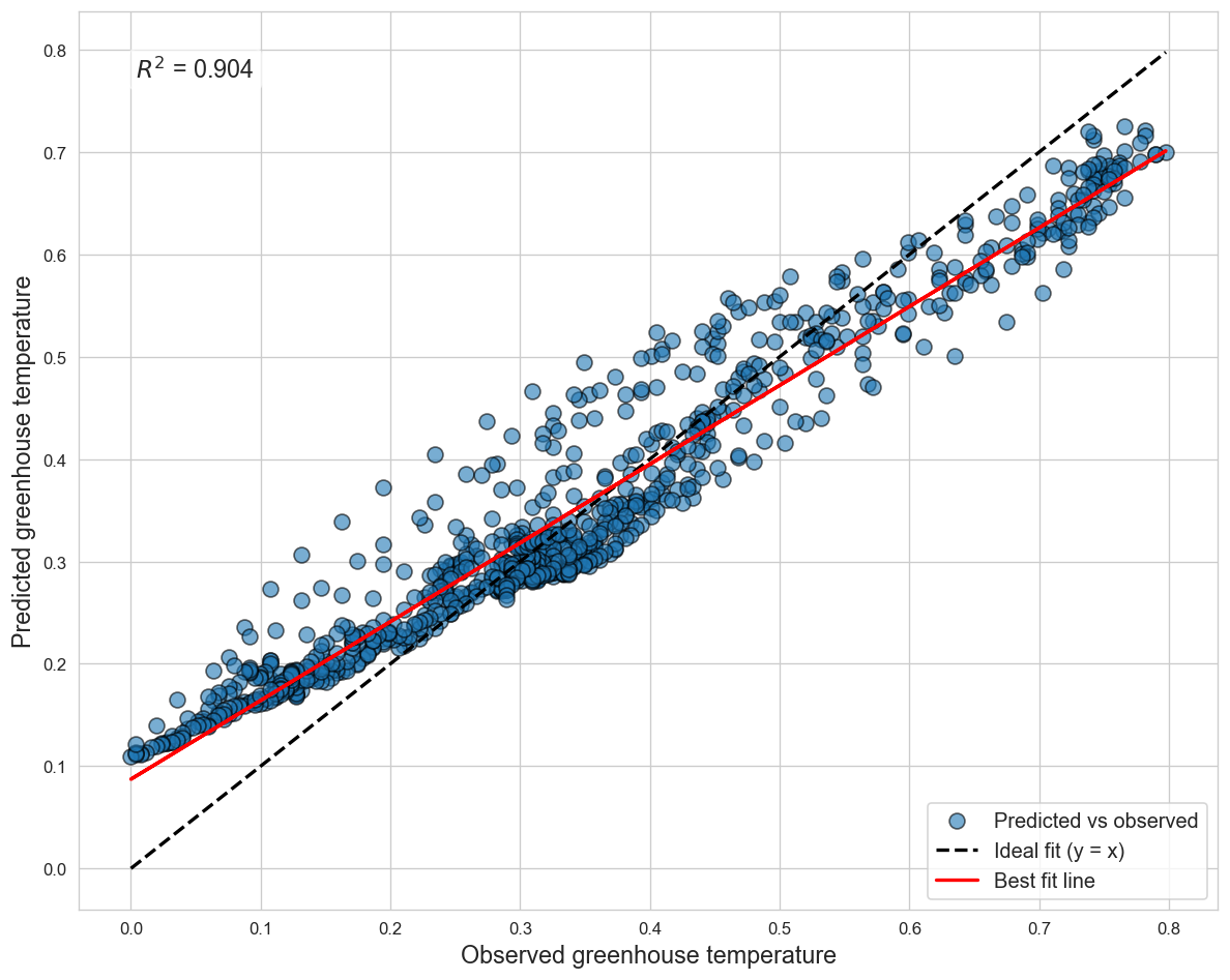
Figure 15: Scatter plot of the observed vs. predicted greenhouse temperature for the autumn period using the STGNN model.

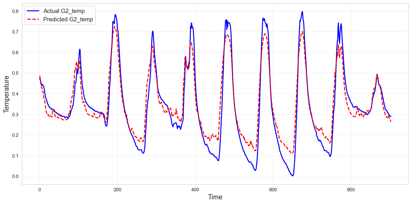
Figure 16: Time series of the observed and predicted greenhouse temperature for the autumn period using the STGNN model.

A.2 Supplementary tables

A.2.1 ADF test results tables

Hypotheses

• $\mbox{H}_{0}$: The series has a unit root (non-stationary),

• $\mbox{H}_{1}$: The series is stationary.

Table 4: ADF test results for stationarity for the summer period

Variable	Dickey-Fuller Statistic	p-value	Conclusion
G2_temp	-15.855	<0.01	Stationary
G2_RH	-11.471	<0.01	Stationary
OUT_temp	-21.311	<0.01	Stationary
OUT_RH	-16.621	<0.01	Stationary
OUT_rad	-21.836	<0.01	Stationary
OUT_wind_speed	-15.131	<0.01	Stationary

Table 5: ADF test results for stationarity for the autumn period

Variable	Dickey-Fuller Statistic	p-value	Conclusion
G2_temp	-16.11	<0.01	Stationary
G2_RH	-13.328	<0.01	Stationary
OUT_temp	-14.324	<0.01	Stationary
OUT_RH	-15.253	<0.01	Stationary
OUT_rad	-17.418	<0.01	Stationary
OUT_wind_speed	-10.395	<0.01	Stationary

Table 6: ADF test results for stationarity for the winter period

Variable	Dickey-Fuller Statistic	p-value	Conclusion
G2_temp	-18.623	<0.01	Stationary
G2_RH	-14.903	<0.01	Stationary
OUT_temp	-13.869	<0.01	Stationary
OUT_RH	-13.673	<0.01	Stationary
OUT_rad	-17.356	<0.01	Stationary
OUT_wind_speed	-9.815	<0.01	Stationary

References

- Abdel-Ghany & Kozai (2006) Abdel-Ghany, A. M., & Kozai, T. (2006). Dynamic modeling of the environment in a naturally ventilated, fog-cooled greenhouse. Renewable Energy, 31, 1521–1539. URL: https://www.sciencedirect.com/science/article/pii/S0960148105002521. doi:https://doi.org/10.1016/j.renene.2005.07.013.
- Alaimo & Seri (2021) Alaimo, L., & Seri, E. (2021). Monitoring the main aspects of social and economic life using composite indicators. a literature review. Research Group Economics, Policy Analysis and Language (REAL) series, .
- Alaoui et al. (2023) Alaoui, M. E., Chahidi, L. O., Rougui, M., Mechaqrane, A., & Allal, S. (2023). Evaluation of cfd and machine learning methods on predicting greenhouse microclimate parameters with the assessment of seasonality impact on machine learning performance. Scientific African, 19, e01578. doi:https://doi.org/10.1016/j.sciaf.2023.e01578.
- Baglivo et al. (2020) Baglivo, C., Mazzeo, D., Panico, S., Bonuso, S., Matera, N., Congedo, P. M., & Oliveti, G. (2020). Complete greenhouse dynamic simulation tool to assess the crop thermal well-being and energy needs. Applied Thermal Engineering, 179, 115698. URL: https://www.sciencedirect.com/science/article/pii/S135943112033180X. doi:https://doi.org/10.1016/j.applthermaleng.2020.115698.
- Behrang et al. (2010) Behrang, M., Assareh, E., Ghanbarzadeh, A., & Noghrehabadi, A. (2010). The potential of different artificial neural network (ann) techniques in daily global solar radiation modeling based on meteorological data. Solar Energy, 84, 1468–1480. doi:https://doi.org/10.1016/j.solener.2010.05.009.
- Belhaj Salah & Fourati (2021) Belhaj Salah, L., & Fourati, F. (2021). A greenhouse modeling and control using deep neural networks. Applied Artificial Intelligence, 35, 1905–1929. doi:10.1080/08839514.2021.1995232.
- Brækken et al. (2023) Brækken, A., Sannan, S., Jerca, I. O., & Bădulescu, L. A. (2023). Assessment of heating and cooling demands of a glass greenhouse in bucharest, romania. Thermal Science and Engineering Progress, 41, 101830. URL: https://www.sciencedirect.com/science/article/pii/S245190492300183X. doi:https://doi.org/10.1016/j.tsep.2023.101830.
- Bussab et al. (2007) Bussab, M. A., Bernardo, J. I., & Hirakawa, A. R. (2007). Greenhouse modeling using neural networks. In World Scientific and Engineering Academy and Society (WSEAS) AIKED’07 (p. 131–135). Stevens Point, Wisconsin, USA. doi:10.5555/1348485.1348508.
- Cheung & Lai (1995) Cheung, Y.-W., & Lai, K. S. (1995). Lag order and critical values of the augmented dickey-fuller test. Journal of Business & Economic Statistics, 13, 277–280. URL: http://www.jstor.org/stable/1392187.
- Dae-Hyun et al. (2020) Dae-Hyun, J., Hyoung, S. K., Changho, J., Hak-Jin, K., & Soo, H. P. (2020). Time-serial analysis of deep neural network models for prediction of climatic conditions inside a greenhouse. Computers and Electronics in Agriculture, 173, 105402. doi:https://doi.org/10.1016/j.compag.2020.105402.
- Dubinin & Effenberger (2024) Dubinin, I., & Effenberger, F. (2024). Fading memory as inductive bias in residual recurrent networks. Neural Networks, 173, 106179. doi:10.1016/j.neunet.2024.106179.
- D’Emilio et al. (2012) D’Emilio, A., Mazzarella, R., Porto, S. M. C., & Cascone, G. (2012). Neural networks for predicting greenhouse thermal regimes during soil solarization. Transactions of the ASABE, 55, 1093–1103. URL: https://api.semanticscholar.org/CorpusID:110002384.
- Escamilla-García et al. (2020) Escamilla-García, A., Soto-Zarazúa, G. M., Toledano-Ayala, M., Rivas-Araiza, E., & Gastélum-Barrios, A. (2020). Applications of artificial neural networks in greenhouse technology and overview for smart agriculture development. Applied Sciences, 10. doi:10.3390/app10113835.
- Ferreira et al. (2002) Ferreira, P., Faria, E., & Ruano, A. (2002). Neural network models in greenhouse air temperature prediction. Neurocomputing, 43, 51–75. doi:https://doi.org/10.1016/S0925-2312(01)00620-8. Selected engineering applications of neural networks.
- Fitz-Rodríguez et al. (2010) Fitz-Rodríguez, E., Kubota, C., Giacomelli, G. A., Tignor, M. E., Wilson, S. B., & McMahon, M. (2010). Dynamic modeling and simulation of greenhouse environments under several scenarios: A web-based application. Computers and Electronics in Agriculture, 70, 105–116. URL: https://www.sciencedirect.com/science/article/pii/S0168169909001902. doi:https://doi.org/10.1016/j.compag.2009.09.010.
- Fourati & Chtourou (2007) Fourati, F., & Chtourou, M. (2007). A greenhouse control with feed-forward and recurrent neural networks. Simulation Modelling Practice and Theory, 15, 1016–1028. doi:https://doi.org/10.1016/j.simpat.2007.06.001.
- Gao et al. (2023) Gao, M., Wu, Q., Li, J., Wang, B., Zhou, Z., Liu, C., & Wang, D. (2023). Temperature prediction of solar greenhouse based on narx regression neural network. Scientific Reports, 13, 1563. doi:https://doi.org/10.1038/s41598-022-24072-1.
- Gharghory (2020) Gharghory, S. M. (2020). Deep network based on long short-term memory for time series prediction of microclimate data inside the greenhouse. International Journal of Computational Intelligence and Applications, 19, 2050013. doi:10.1142/S1469026820500133.
- Goodfellow et al. (2016) Goodfellow, I., Bengio, Y., & Courville, A. (2016). Sequence modeling: Recurrent and recursive nets. In Deep Learning chapter 10. MIT Press. URL: http://www.deeplearningbook.org.
- Guo et al. (2020) Guo, Y., Zhao, H., Zhang, S., Wang, Y., & Chow, D. (2020). Modeling and optimization of environment in agricultural greenhouses for improving cleaner and sustainable crop production. Journal of Cleaner Production, (p. 124843). URL: https://api.semanticscholar.org/CorpusID:228963541.
- Hochreiter & Schmidhuber (1997) Hochreiter, S., & Schmidhuber, J. (1997). Long short-term memory. Neural Computation, 9, 1735–1780. doi:10.1162/neco.1997.9.8.1735.
- Hongkang et al. (2018) Hongkang, W., Li, L., Yong, W., Fanjia, M., Haihua, W., & Sigrimis, N. (2018). Recurrent neural network model for prediction of microclimate in solar greenhouse. IFAC-PapersOnLine, 51, 790–795. doi:10.1016/j.ifacol.2018.08.099. 6th IFAC Conference on Bio-Robotics BIOROBOTICS 2018.
- Jain & Medsker (1999) Jain, L. C., & Medsker, L. R. (1999). Recurrent Neural Networks: Design and Applications. (1st ed.). USA: CRC Press, Inc. doi:10.5555/553011.
- Jin et al. (2024) Jin, M., Koh, H. Y., Wen, Q., Zambon, D., Alippi, C., Webb, G. I., King, I., & Pan, S. (2024). A survey on graph neural networks for time series: Forecasting, classification, imputation, and anomaly detection. IEEE Transactions on Pattern Analysis and Machine Intelligence, 46, 10466–10485. doi:10.1109/TPAMI.2024.3443141.
- Kingma & Ba (2014) Kingma, D., & Ba, J. (2014). Adam: A method for stochastic optimization. In International Conference on Learning Representations. doi:10.48550/arXiv.1412.6980.
- Kirchgässner et al. (2012) Kirchgässner, G., Wolters, J., & Hassler, U. (2012). Introduction to modern time series analysis. (2nd ed.). Heidelberg: Springer Berlin. doi:10.1007/978-3-642-33436-8.
- Malvar et al. (2004) Malvar, H. S., He, L.-w., & Cutler, R. (2004). High-quality linear interpolation for demosaicing of bayer-patterned color images. In 2004 IEEE International Conference on Acoustics, Speech, and Signal Processing (pp. iii–485). IEEE volume 3.
- Manonmani et al. (2018) Manonmani, A., Thyagarajan, T., Elango, M., & Sutha, S. (2018). Modelling and control of greenhouse system using neural networks. Transactions of the Institute of Measurement and Control, 40, 918 – 929. URL: https://api.semanticscholar.org/CorpusID:125880926.
- Mobtaker et al. (2019) Mobtaker, H. G., Ajabshirchi, Y., Ranjbar, S. F., & Matloobi, M. (2019). Simulation of thermal performance of solar greenhouse in north-west of iran: An experimental validation. Renewable Energy, 135, 88–97. URL: https://www.sciencedirect.com/science/article/pii/S096014811831187X. doi:https://doi.org/10.1016/j.renene.2018.10.003.
- Nielsen (2015) Nielsen, M. A. (2015). Neural networks and deep learning volume 25. Determination press San Francisco, CA, USA.
- Nketiah et al. (2023) Nketiah, E. A., Chenlong, L., Yingchuan, J., & Aram, S. A. (2023). Recurrent neural network modeling of multivariate time series and its application in temperature forecasting. Plos one, 18, e0285713. doi:10.1371/journal.pone.0285713.
- Ouazzani Chahidi et al. (2021) Ouazzani Chahidi, L., Fossa, M., Priarone, A., & Mechaqrane, A. (2021). Energy saving strategies in sustainable greenhouse cultivation in the mediterranean climate – a case study. Applied Energy, 282, 116156. URL: https://www.sciencedirect.com/science/article/pii/S0306261920315646. doi:https://doi.org/10.1016/j.apenergy.2020.116156.
- Patil et al. (2008) Patil, S., Tantau, H., & Salokhe, V. (2008). Modelling of tropical greenhouse temperature by auto regressive and neural network models. Biosystems Engineering, 99, 423–431. doi:https://doi.org/10.1016/j.biosystemseng.2007.11.009.
- Petrakis et al. (2022) Petrakis, T., Kavga, A., Thomopoulos, V., & Argiriou, A. A. (2022). Neural network model for greenhouse microclimate predictions. Agriculture, . URL: https://api.semanticscholar.org/CorpusID:249187802.
- Rodriguez et al. (1999) Rodriguez, P., Wiles, J., & Elman, J. L. (1999). A recurrent neural network that learns to count. Connection Science, 11, 5–40. doi:10.1080/095400999116340.
- Salah & Fourati (2021) Salah, L. B., & Fourati, F. (2021). A greenhouse modeling and control using deep neural networks. Applied Artificial Intelligence, 35, 1905 – 1929. URL: https://api.semanticscholar.org/CorpusID:240019305.
- Seginer et al. (1994) Seginer, I., Boulard, T., & Bailey, B. (1994). Neural network models of the greenhouse climate. Journal of Agricultural Engineering Research, 59, 203–216. doi:https://doi.org/10.1006/jaer.1994.1078.
- Singh et al. (2018) Singh, M. C., Singh, J., & Singh, K. (2018). Development of a microclimate model for prediction of temperatures inside a naturally ventilated greenhouse under cucumber crop in soilless media. Computers and Electronics in Agriculture, 154, 227–238. URL: https://www.sciencedirect.com/science/article/pii/S016816991830022X. doi:https://doi.org/10.1016/j.compag.2018.08.044.
- Stanciu et al. (2016) Stanciu, C., Stanciu, D., & Dobrovicescu, A. (2016). Effect of greenhouse orientation with respect to e-w axis on its required heating and cooling loads. Energy Procedia, 85, 498–504. URL: https://www.sciencedirect.com/science/article/pii/S1876610215028994. doi:https://doi.org/10.1016/j.egypro.2015.12.234. EENVIRO-YRC 2015 - Bucharest.
- Sun et al. (2022) Sun, L., Liu, T., Wang, D., Huang, C., & Xie, Y. (2022). Deep learning method based on graph neural network for performance prediction of supercritical co2 power systems. Applied Energy, 324, 119739. doi:https://doi.org/10.1016/j.apenergy.2022.119739.
- Taewon et al. (2019) Taewon, M., Seojung, H., Ha, Y. C., Dae, H. J., Se, H. C., & Jung, E. S. (2019). Interpolation of greenhouse environment data using multilayer perceptron. Computers and Electronics in Agriculture, 166, 105023. doi:https://doi.org/10.1016/j.compag.2019.105023.
- Tsay (2005) Tsay, R. S. (2005). Analysis of financial time series. John wiley & sons.
- Vaswani et al. (2017) Vaswani, A., Shazeer, N., Parmar, N., Uszkoreit, J., Jones, L., Gomez, A. N., Kaiser, L., & Polosukhin, I. (2017). Attention is all you need. In Proceedings of the 31st International Conference on Neural Information Processing Systems NIPS’17 (p. 6000–6010). Red Hook, NY, USA: Curran Associates Inc. doi:10.5555/3295222.3295349.
- Veličković et al. (2018) Veličković, P., Cucurull, G., Casanova, A., Romero, A., Lio, P., & Bengio, Y. (2018). Graph attention networks. In International Conference on Learning Representations (ICLR). doi:10.48550/arXiv.1710.10903.
- Yu et al. (2018) Yu, B., Yin, H., & Zhu, Z. (2018). Spatio-temporal graph convolutional networks: A deep learning framework for traffic forecasting. In Proceedings of the Twenty-Seventh International Joint Conference on Artificial Intelligence, IJCAI-18 (pp. 3634–3640). International Joint Conferences on Artificial Intelligence Organization. doi:10.24963/ijcai.2018/505.