On a class of high dimensional linear regression methods with debiasing and thresholding

Abstract

In this paper, we introduce a unified framework, inspired by classical regularization theory, for designing and analyzing a broad class of linear regression approaches. Our framework encompasses traditional methods like least squares regression and Ridge regression, as well as innovative techniques, including seven novel regression methods such as Landweber and Showalter regressions. Within this framework, we further propose a class of debiased and thresholded regression methods to promote feature selection, particularly in terms of sparsity. These methods may offer advantages over conventional regression techniques, including Lasso, due to their ease of computation via a closed-form expression. Theoretically, we establish consistency results and Gaussian approximation theorems for this new class of regularization methods. Extensive numerical simulations further demonstrate that the debiased and thresholded counterparts of linear regression methods exhibit favorable finite sample performance and may be preferable in certain settings.

Keywords: Linear regression, regularization, consistency, Gaussian approximation, sparsity, debias, threshold

1 Introduction

In a regression setting, suppose the observations are $\left\{(X_{i1},\cdots,X_{ip},Y_{i})\right\}\in\mathbf{R}^{p}\times\mathbf{R}$ for $i=1,2,\cdots,n$, fitting a linear model

$$Y_{i}=\sum_{j=1}^{p}X_{ij}\beta_{j}+e_{i},\ \text{with }e_{i}\ \text{being i.i.d. and }\mathbf{E}e_{i}=0,$$ (1)

remains a strong candidate despite the availability of more complex models like regression trees, neural networks, non-parametric regression techniques, among others, due to the linear model’s good interpretability and low computational costs. Furthermore, in situations where data collection is expensive or the data exhibit high dimensionality (i.e., when $p$ is comparable to or even larger than $n$), nonlinear regression models like those introduced in Bartlett et al. (2019) may incur high model complexities, and suffer from the curse of dimensionality. In such cases, feature selection techniques, such as those proposed by Radchenko and James (2010) and Li et al. (2012), become essential prior to model fitting. However, these techniques can introduce selection bias, and potentially reduce the interpretability of the model.

This paper aims to establish a unified theoretical framework for analyzing various high-dimensional linear regression methods, including both traditional techniques like Ridge regression and newer approaches such as Landweber regression (Wang et al., 2024, Example 3.3) and Showalter regression (Wang et al., 2024, Example 3.4), among others, in situations where $p\approx n$. While extensive research has been conducted to Lasso and its variants in high-dimensional settings, to our knowledge, there is a relative lack of studies on alternative linear regression methods. This has led to limited options for theoretically robust approaches that address different kinds of practical applications. The results presented in this paper provide practitioners with the tools to perform statistical inference across a wide range of linear regression methods, thereby expanding the available choices of linear regression methods for practical implementation. Beyond the simplification of theoretical study of existing linear regression methods, the propose of our work also establishes a basis for generating new regression methods that may be more efficient in practice for various regression problems.

Remark 1.

Conducting linear regression under the scenario of $p\approx n$ is common in practical applications. To mention few examples, the work of Batenburg et al. (2021) in X-ray-based computerized tomography (CT), Zhang et al. (2016) in gas leak localization, Wang et al. (2013) in extinction spectrometry for determining atmospheric aerosol size characteristics, Dassios and Fokas (2020) in electroencephalogram/magnetoencephalography (EEG/MEG) analysis, Hosseini and Plataniotis (2020) in image deblurring, Zhang et al. (2018a) in determination of rate constants in biochemical and pharmacological reactions, among others, adopted integral equations when constructing mathematical models. The Cauchy problem and data completion mentioned in Huang et al. (2023), the diffusion-based bioluminescence tomography introduced in Gong et al. (2020), and the inverse source problems in mathematical physics as mentioned in Zhang and Gong (2020), relied on solving inverse problems for partial differential equations. For integral equations or partial differential equations seldom have close–form solutions, numerical methods, which involve discretization of these equations, becomes essential to solve the system. The discretization of these equations frequently results in linear models (1) with $p\approx n$.

Compared to the widely studied setting where $p\gg n$, the setting where $p\approx n$ presents unique challenges. In particular, the design matrix $X$ can become ill-conditioned and have an extremely large condition number (cond$(X)$), which may diverge to infinity as the sample size $n\to\infty$. Blindly applying commonly used linear regression methods, such as least squares estimation, in this scenario can lead to estimators with high variances. While there are regression algorithms designed to handle ill-conditioned $X$, the theoretical analysis of these methods remains lacking and often case-specific. Our work aims to provide practitioners with a general theoretical framework for analyzing these algorithms.

Another motivation arises from recent advancements and challenges in the field of inverse problems. Significant progress has been made in regularization methods and theories over the past few decades, as seen in the works of (Engl et al., 1996; Kaipio and Somersalo, 2005; Ito and Jin, 2014; Benning and Burger, 2018). In contrast to traditional Tikhonov regularization, also known as Ridge regression in statistics, many new regularization methods have been developed for various purposes, such as sparse promotion (Li, 2023; Grasmair et al., 2008; Chen et al., 2016; Lorenz and Resmerita, 2016; Ding and Han, 2019; Daubechies et al., 2016), edge preservation (Stefan et al., 2010; Guo et al., 2014; Zhang et al., 2017; Weinmann et al., 2014; Tong et al., 2018), structure preservation (Droske and Bertozzi, 2010; Bardsley and Hansen, 2020; Zhang and Hofmann, 2021), positivity preservation (Bardsley and Hansen, 2020; Zhang and Hofmann, 2021), higher-Order feature preservation (Droske and Bertozzi, 2010), acceleration (Zhang, 2023; Jiao et al., 2017), uncertainty quantification (Flath et al., 2011; Ernst et al., 2015; Alexanderian et al., 2021; Zhang and Chen, 2022), among others. However, due to differing mathematical frameworks, these new regularization methods have not garnered widespread attention in the statistical community. Thanks to developments in machine learning, the combination of statistics and inverse problems is now being leveraged to create new algorithms for regression problems.

This paper aims to address the challenges of high-dimensional and ill-posed problems, where traditional techniques like least squares and Ridge regression are often ineffective. In inverse problems, regularization methods are typically applied before discretization to manage the ill-posedness of the original infinite-dimensional models. These regularization techniques are generally dimensionless, allowing them to offer superior linear regression estimates, especially in cases with ill-conditioned matrices where $p\approx n\gg 1$. Building on the theory of general linear regularization (Lu and Pereverzev, 2013) and modern regularization theory in inverse problems (as discussed in Mathé and Pereverzev (2003) or (Zhang and Hofmann, 2019, Section 2)), we extend the statistical framework presented in Wang et al. (2024) for general linear regression to encompass infinite-dimensional cases, which are characterized by the following simple structure:

$$\frac{1}{n}g_{\alpha}(\frac{1}{n}\mathbf{X}_{n}^{\textrm{T}}\mathbf{X}_{n})\mathbf{X}_{n}^{\textrm{T}}\mathbf{Y}_{n},$$ (2)

where $g_{\alpha}$ is a linear function that satisfies the three conditions in Definition 1 in the following section. Additionally, building on this framework to enhance model selection, we develop a class of debiased and thresholded linear regression methods and establish both a consistency theorem and a Gaussian approximation theorem. It is important to note that we do not require the explicit formula for the function $g_{\alpha}$ when designing a concrete regression method; see Section 3.2 for demonstrations. Instead, we only need certain properties of $g_{\alpha}$ to study the statistical properties of a broad class of regression methods, which exhibit the structure described in (2).

In summary, our work addresses parameter selection, estimation, and inference in a linear model where the number of parameters $p$ approximately equals sample size $n$. In addition, we explore its potential applications in solving inverse source problems. The main contributions include the following aspects:

• Model selection procedure: A frequent issue raised in penalized regression methods involves selecting optimal regularization parameters. To address these issues, we introduce a set of new iterative algorithms within our unified regression framework, shifting the focus from parameter selection to determining appropriate iteration steps using effective termination criteria, while maintaining the same order of accuracy. Numerical experiments indicate that a simple a posteriori stopping rule (i.e., the discrepancy principle) can make our novel iterative regression methods highly efficient, often yielding satisfactory or even superior results without additional computational costs.

• Debiasing & Thrsholding gyhystrategy for various linear regression methods: Debiasing is an essential step when performing statistical inference for high-dimensional regression, as emphasized in works of Zhang and Zhang (2014) and Chernozhukov et al. (2018), due to the large bias that may arise. In fact, in certain situations, the magnitude of bias can even exceed that of the random errors. In this paper, we compute the debiased regression estimator for the proposed class of regularized linear regression methods. In addition, we introduce thresholding techniques to enhance variable selection accuracy and preserve the sparsity of the estimator. This combined debiasing and thresholding procedure facilitates valid statistical inference.

• Gaussian approximation theorem & bootstrap algorithm for statistical inference: The limiting behavior of the proposed estimator is analyzed through a Gaussian approximation theorem. For the proposed estimator does not follow a standard asymptotic distribution, a bootstrap algorithm is employed to facilitate statistical inference.

The remainder of the paper is organized as follows: in the first part of Section 3, we present the definition of the generator (i.e., the function $g_{\alpha}$ in (2)) of linear regression methods, after which, we introduce frequently used notation and assumptions. The subsequent portion of Section 3 delves into the examination of various properties of the proposed linear regression methods, including consistency, the Gaussian approximation theorem, and best-worst-case error analysis. Section 3.2 is dedicated to demonstrating the application of our theory. Here, we present nine examples of linear regression methods covered by our framework, comprising two conventional linear regression methods and seven newly developed alternatives. Section 6 presents numerical experiments along with a comparison with nine regression methods. Finally, concluding remarks are given in Section 7, and technical proofs of assertions are provided in the Appendices.

2 Related literature

The study of linear regression dates back to the 1890s, when Pearson (1896) expanded on the concept of regression coined by Galton (1886) and provided the mathematical foundation for the regression model. In recent years, there has been a growing body of literature focusing on the theoretical properties of linear regression in high-dimensional settings. Among these studies, the development and analysis of regularization techniques to improve estimation accuracy have been extensively explored. We divide the discussion into two parts: inverse problems and statistics.

  Inverse Problem

The practical significance of general ill-posed problems, formulated as operator equations, was first highlighted by Tikhonov in his seminal papers Tikhonov (1963a, b). In these papers, Tikhonov also introduced the concept of conditionally well-posed problems and the idea of regularization algorithms, which have played a crucial role in the development of the theory and applications of such problems. This approach incorporates a regularization parameter that strikes a balance between stability and accuracy by imposing constraints during the solution process. The formulation of ill-posed equations and the development of specialized methods for their solutions were explored by Lavret’ev (1953, 1959); Ivanov (1962, 1963); Phillips (1962), among others, during the last decades of the 20th century. Modern regularization theory for ill-posed inverse problems is extensively covered in well-known monographs by Tichonov et al. (1998); Ivanov et al. (2002); Engl et al. (1996); Ito and Jin (2014), and many others. Morozov (1966) introduced the ”Morozov discrepancy principle,” a key criterion for selecting regularization parameters, which has become a widely used method for this purpose. Bakushinsky and Kokurin (2004); Kaltenbacher et al. (2008) systematically studied iterative regularization methods for solving operator equations, while the finite-dimensional analog has been intensively investigated by Hansen (2010). Vainikko and Veretennikov (1986) was the first to study a broad class of regularization methods within a unified framework. Mathé (2004) demonstrated the saturation of methods for solving linear ill-posed problems in Hilbert spaces by introducing the concept of qualification for a wide class of regularization methods. Hofmann and Mathé (2007) proposed a general framework for regularization methods, which inspired and laid the foundation for the linear regression framework developed in Section 3. It is worth noting that although we adopt the same framework of methods, our focus is fundamentally different: while the previous studies in inverse problems emphasize the perturbation theory of regularization methods, our interest lies in their statistical properties.

  High–dimensional linear regression

Analyzing a linear model under the presence of high–dimensionality has been extensively explored in the literature. Some notable results include Fan and Li (2001), Zhao and Yu (2006) for (model–selection) consistency, Bühlmann (2013), Zhang and Zhang (2014) and Guo and Cheng (2022), Li and Li (2022), for statistical inference, and Martin and Tang (2020) for Bayesian inference. Mammen (1993), Lopes (2014), Zhang and Politis (2020), among others, introduced bootstrap algorithm to assist statistical inference and prediction. The work of Chronopoulos et al. (2022) and Zhang and Politis (2023) discussed high–dimensional linear model for dependent and heterogeneous data. We also refer the textbooks by Bühlmann and van de Geer (2011) and Fan et al. (2020) for a complete introduction.

Among linear regression methods, the Lasso algorithm proposed by Tibshirani (1996) has become the main work-horse for high-dimensional sparse linear model, due to its implicitly zeroing out of insignificant regression coefficients, as introduced by Knight and Fu (2000) and Tibshirani (1996). However, in practice the zeroing effect can not be guaranteed for the optimization algorithms used in Lasso, such as stochastic gradient descent, may stop early before reaching the minimizer. To solve this issue, (van de Geer et al., 2011, Section 7) further thresholded the estimated Lasso coefficients, making a guaranteed sparse fitted model. In addition to Lasso, the idea of thresholding is applied to other linear regression algorithms such as ridge regression, as mentioned in Zhang and Politis (2020) and Zhang and Politis (2023).

While performing linear regression in the low- and high-dimensional setting has been extensively studied, regression in scenarios where $p\approx n$ has received comparatively little attention. However, as discussed in the introduction section, recent advances in the fields of inverse problems and computational physics have highlighted new challenges, and regression in the $p\approx n$ setting introduces additional complexities. Concerning this context, we believe that addressing these challenges could be beneficial for a board range of physical problems in complex and random media, including but not limited to the data completion problem in mathematical physics (Dou et al. (2022)), biosensor data analysis (Zhang et al. (2019)), and bioluminescence tomography (Gong et al. (2020)); inverse random source problems for stochastic acoustic, biharmonic, electromagnetic, and elastic wave equations (Li et al. (2022); Bao and Li (2022)), sonar localization problems (Frese et al. (2005); Meng and Zhang (2024)), and aerosol science and technology (Wang et al. (2013); Naseri et al. (2021)).

3 Debiasing and thresholding in linear regression

This manuscript focuses on the high-dimensional linear regression model

$$\mathbf{Y}_{n}=\mathbf{X}_{n}\boldsymbol{\beta}+\boldsymbol{e}_{n},$$ (3)

where $\mathbf{Y}_{n}=[Y_{1},\dots,Y_{n}]^{\textrm{T}}\in\mathbf{R}^{n}$ represents the response vector, $\mathbf{X}_{n}=[x_{ij}]_{1\leq i\leq n,1\leq j\leq p}\in\mathbf{R}^{n\times p}$ denotes the fixed (non-random) design matrix, which is assumed to have rank $s=s(n,p)$ and may grow unbounded as $n,p\to\infty$. $\boldsymbol{\beta}=[\beta_{1},\dots,\beta_{p}]^{\textrm{T}}\in\mathbf{R}^{p}$ represents the vector of coefficients to be estimated. $\boldsymbol{e}_{n}=[e_{1},\dots,e_{n}]^{\textrm{T}}\in\mathbf{R}^{n}$ denotes the error vector.

3.1 A class of linear regression methods

The exploration begins by introducing the generator function $g_{\alpha}(\cdot)$ in (2), which is analogous to our recent work in Wang et al. (2024) on low-dimensional linear regression. The initial idea of using a parametric spectral function $g_{\alpha}(\cdot)$ was first introduced in the monograph Zhang and Hofmann (2019) within the context of regularization theory for inverse problems. In that work, a pair of functions $(g_{\alpha}(\lambda),r_{\alpha}(\lambda))$ was used to systematically study the convergence properties of some simple variational and iterative regularization methods. This pair of functions plays a crucial role in the convergence analysis of regularization methods, revealing the structure described in (2). Building on the specific geometry of the class of functions $g_{\alpha}(\cdot)$ Mathé and Pereverzev (2003) and Hofmann and Mathé (2007) investigated the convergence rate results for ill-posed linear inverse problems in a unified framework. Over the past five years, many researchers in the field of inverse problems, such as Boţ et al. (2022); Zhang and Hofmann (2019, 2020), have extended this framework to study the convergence rate results for more complex modern regularization methods.

Definition 1.

A family of functions $g_{\alpha}(\lambda)$ $(\lambda>0)$, defined for regression parameters $0\leq\alpha\leq\overline{\alpha}$, constitutes a generator of linear regression methods for problem (3) if the following three conditions are satisfied:

1. For the bias function $r_{\alpha}(\lambda):=1-\lambda g_{\alpha}(\lambda)$, it holds that for any fixed $\lambda\in(0,+\infty]$ the limit condition $\lim\limits_{\alpha\to 0}|r_{\alpha}(\lambda)|=0$.

2. There exists a constant $c_{r}>0$ such that $|r_{\alpha}(\lambda)|\leq c_{r}$ for all $\lambda\in(0,+\infty]$ and $\alpha\in(0,\overline{\alpha}]$.

3. There exists a constant $c_{0}>0$ such that $g_{\alpha}(\lambda)\leq\min(2/\lambda,c_{0}/\sqrt{\lambda\alpha})$ for all $\lambda\in(0,+\infty]$ and $\alpha\in(0,\overline{\alpha}]$.

By selecting a suitable generator function $g_{\alpha}(\lambda)$, practitioners can derive a class of linear regression methods parameterized by $\alpha$ through the following expression:

$$\hat{\boldsymbol{\beta}}_{\alpha}=\frac{1}{n}g_{\alpha}(\frac{1}{n}\mathbf{X}_{n}^{\textrm{T}}\mathbf{X}_{n})\mathbf{X}_{n}^{\textrm{T}}\mathbf{Y}_{n}.$$ (4)

When the parameter vector $\boldsymbol{\beta}$ is of comparable dimension to the sample size $n$, the bias introduced during model-fitting is always large compared to the random errors, as introduced in Zhang and Zhang (2014); Chernozhukov et al. (2018); Zhang and Politis (2020). This can result in an inconsistent estimator or significantly reduce the coverage probability of confidence intervals. Therefore, as discussed in Section 4, it becomes necessary to eliminate this bias before performing statistical inference. While eliminating bias is generally a hard problem according to Chernozhukov et al. (2018), a closed-form debiased estimator can be derived in our setting. This estimator is detailed below and in equation (24) in Section 4.

$$\tilde{\boldsymbol{\beta}}_{\alpha}=\frac{1}{n}\left[I+r_{\alpha}(\frac{1}{n}\mathbf{X}_{n}^{\textrm{T}}\mathbf{X}_{n})\right]g_{\alpha}(\frac{1}{n}\mathbf{X}_{n}^{\textrm{T}}\mathbf{X}_{n})\mathbf{X}_{n}^{\textrm{T}}\mathbf{Y}_{n}.$$

Definition 2 (Slightly modified from Definition 2.3 in Zhang and Hofmann (2020)).

A linear regression method (4) for equation (3) generated by the generator function $g_{\alpha}(\lambda)(0<\lambda\leq C_{\lambda})$ is said to have a monomial qualification of order $d$ if the following inequality holds

$$\sup_{\lambda\in\left(0,C_{\lambda}\right]}\left|r_{\alpha}(\lambda)\right|\lambda^{d}\leq C_{*}\alpha^{d},$$ (5)

where $C_{\lambda}$ and $C_{*}$ are constants independent of the value of $\alpha$.

Remark 2.

Definition 1 and 2 are both useful and have been extensively discussed in the realms of inverse problems and regularization, as extensively demonstrated in (Engl et al., 1996). However, to the best of our knowledge, despite their widespread practical application, the framework of Definition 1 and 2 has seldom been theoretically adopted in the regression scenario, particularly when considering the presence of noise and high-dimensionality. Therefore, this manuscript utilizes the framework of Definition 1 and 2 to perform regression and provides practitioners with theoretical guarantees.

With a given positive threshold $b_{n}$ (the subscript stresses the value of $b_{n}$ may change with respect to sample size), we adopt the notation $\mathcal{N}_{b_{n}}$ to denote the set of indices whose corresponding elements are larger than $b_{n}$ in absolute values, i.e., $\mathcal{N}_{b_{n}}=\left\{i||\beta_{i}|>b_{n}\right\}$. Similarly, we define the index sets $\widehat{\mathcal{N}}_{b_{n}}$ and $\widetilde{\mathcal{N}}_{b_{n}}$, the thresholded estimator $\hat{\boldsymbol{\theta}}=\left(\hat{\theta}_{1},\cdots,\hat{\theta}_{p}\right)^{\textrm{T}}$ and the thresholded debiased estimator $\tilde{\boldsymbol{\theta}}=\left(\tilde{\theta}_{1},\cdots,\tilde{\theta}_{p}\right)^{\textrm{T}}$ as follows:

$$\widehat{\mathcal{N}}_{b_{n}}=\left\{i||(\hat{\boldsymbol{\beta}}_{\alpha})_{i}|>b_{n}\right\},\quad\hat{\theta}_{i}=(\hat{\boldsymbol{\beta}}_{\alpha})_{i}\times\boldsymbol{\mathbf{1}}_{i\in\widehat{\mathcal{N}}_{b_{n}}},$$ (6)

$$\widetilde{\mathcal{N}}_{b_{n}}=\left\{i||(\tilde{\boldsymbol{\beta}}_{\alpha})_{i}|>b_{n}\right\},\quad\tilde{\theta}_{i}=(\tilde{\boldsymbol{\beta}}_{\alpha})_{i}\times\boldsymbol{\mathbf{1}}_{i\in\widetilde{\mathcal{N}}_{b_{n}}}.$$

Intuitively, $\hat{\boldsymbol{\theta}}$ and $\tilde{\boldsymbol{\theta}}$ set the estimated values to zero if their original absolute values are too small. Despite its simplicity, this thresholding operation can improve the performance of the original estimator, particularly when the underlying parameter vector $\boldsymbol{\beta}$ is sparse (i.e., most elements of $\boldsymbol{\beta}$ are zero). The underlying idea here is to mitigate error accumulation. Specifically, due to random errors, $(\hat{\boldsymbol{\beta}}_{\alpha})_{i}$ and $(\tilde{\boldsymbol{\beta}}_{\alpha})_{i}$ are often small but non-zero in absolute value when $\boldsymbol{\beta}_{i}=0$. These small errors, however, can accumulate and result in a large value when calculating the Euclidean distance $\sqrt{\sum_{i=1}^{p}|(\tilde{\boldsymbol{\beta}}_{\alpha})_{i}-\boldsymbol{\beta}_{i}|^{2}}$, as the dimension $p$ is large. By applying thresholding, only a few elements of $\hat{\boldsymbol{\theta}}$ and $\tilde{\boldsymbol{\theta}}$ remain non-zero, thereby reducing the summation term $\sqrt{\sum_{i=1}^{p}|(\hat{\boldsymbol{\theta}}_{\alpha})_{i}-\boldsymbol{\beta}_{i}|^{2}}$.

Deriving the simultaneous confidence interval for the parameter vector $\boldsymbol{\beta}$ is more challenging than constructing confidence intervals for individual elements of the parameter vector. This difficulty arises partly from the complex joint distribution exhibited by the estimator $\widehat{\boldsymbol{\theta}}$, as well as the shape of the simultaneous confidence intervals. This manuscript aims to construct rectangular simultaneous confidence intervals, which are more easily visualized compared to the elliptical intervals discussed in Seber and Lee (2012). However, the construction of rectangle simultaneous confidence intervals depends on the distribution of the maximum statistics $\max\limits_{i=1,\dots,p}\left|\hat{\theta}_{i}-\beta_{i}\right|$ and $\max\limits_{i=1,\dots,p}\left|\tilde{\theta}_{i}-\beta_{i}\right|$, for which closed-form formula exists. Concerning this, we resort to the bootstrap algorithms, as demonstrated in Politis et al. (1999), that performs Monte Carlo simulations to estimate the corresponding quantiles. Inspired by the approaches in Chernozhukov et al. (2013), Zhang and Cheng (2017), and Zhang and Wu (2017), we introduce the wild bootstrap algorithm 1.

Algorithm 1 (Wild bootstrap).

Input: Design matrix $\mathbf{X}_{n}$, dependent variables $\mathbf{Y}_{n}=\mathbf{X}_{n}\boldsymbol{\beta}+\boldsymbol{e}_{n}$, threshold $b_{n}$ , nominal coverage probability $1-\alpha^{*}$, number of bootstrap replicates $B$

1. Calculate $\hat{\boldsymbol{\theta}}$ and $\tilde{\boldsymbol{\theta}}$ defined in (6), along with

   $$\widehat{\sigma}^{2}=\frac{1}{n}\sum_{i=1}^{n}\left(Y_{i}-\sum_{j=1}^{p}x_{ij}\hat{\theta}_{j}\right)^{2}\quad\text{and}\quad\widetilde{\sigma}^{2}=\frac{1}{n}\sum_{i=1}^{n}\left(Y_{i}-\sum_{j=1}^{p}x_{ij}\tilde{\theta}_{j}\right)^{2}.$$ (7)

2. Generate i.i.d. errors $\hat{\boldsymbol{e}}_{n}=\left(\hat{e}_{1},\cdots,\hat{e}_{n}\right)^{\textrm{T}}$ with $\hat{e}_{i},i=1,\cdots,n$ having normal distribution with mean 0 and variance $\widehat{\sigma}^{2}$, then calculate $\hat{\mathbf{Y}}^{*}_{n}=\mathbf{X}_{n}\hat{\boldsymbol{\theta}}+\hat{\boldsymbol{e}}_{n}$. Similarly, $\tilde{\boldsymbol{e}}_{n}$ and $\tilde{\mathbf{Y}}^{*}_{n}$ are generated following the same process.

3. Calculate $\hat{\boldsymbol{\beta}}^{*}_{\alpha}=\frac{1}{n}g_{\alpha}(\frac{1}{n}\mathbf{X}_{n}^{\textrm{T}}\mathbf{X}_{n})\mathbf{X}_{n}^{\textrm{T}}\hat{\mathbf{Y}}^{*}_{n}$ and $\tilde{\boldsymbol{\beta}}^{*}_{\alpha}=\frac{1}{n}[I+r_{\alpha}(\frac{1}{n}\mathbf{X}_{n}^{\textrm{T}}\mathbf{X}_{n})]g_{\alpha}(\frac{1}{n}\mathbf{X}_{n}^{\textrm{T}}\mathbf{X}_{n})\mathbf{X}_{n}^{\textrm{T}}\tilde{\mathbf{Y}}^{*}_{n}$

4. Calculate $\widehat{\mathcal{N}}^{*}_{b_{n}}=\left\{i||(\hat{\boldsymbol{\beta}}^{*}_{\alpha})_{i}|>b_{n}\right\}$ and $\hat{\boldsymbol{\theta}}^{*}=\left(\hat{\theta}^{*}_{1},\cdots,\hat{\theta}^{*}_{p}\right)^{\textrm{T}}$ with $\hat{\theta}^{*}_{i}=(\hat{\boldsymbol{\beta}}_{\alpha})^{*}_{i}\times\boldsymbol{\mathbf{1}}_{i\in\widehat{\mathcal{N}}_{b_{n}}}$ for $i=1,\cdots,p$. Similarly, $\widetilde{\mathcal{N}}^{*}_{b_{n}}$ and $\tilde{\boldsymbol{\theta}}^{*}$

5. Calculate $\hat{E}_{b}^{*}=\max\limits_{i=1,\cdots,p}\left|\hat{\theta}^{*}_{i}-\hat{\theta}_{i}\right|$ and $\tilde{E}_{b}^{*}=\max\limits_{i=1,\cdots,p}\left|\tilde{\theta}^{*}_{i}-\tilde{\theta}_{i}\right|$.

6. (For constructing a confidence region) Repeat steps 2 to 5 for $B$ times to generate $\hat{E}_{b}^{*},\tilde{E}_{b}^{*},b=1,2,\ldots,B$; then calculate the $1-\alpha^{*}$ sample quantile $\hat{C}_{1-\alpha^{*}}^{*}$ of $\hat{E}_{b}^{*}$ and $\tilde{C}_{1-\alpha^{*}}^{*}$ of $\tilde{E}_{b}^{*}$. The $1-\alpha^{*}$ confidence region for the parameter of interest $\boldsymbol{\beta}$ are given by the sets

   $$\left\{\boldsymbol{\beta}=(\beta_{1},\cdots,\beta_{p})^{\textrm{T}}|\max_{i=1,\cdots,p}\left|\hat{\theta}_{i}-\beta_{i}\right|\leq\hat{C}_{1-\alpha^{*}}^{*}\right\}$$ (8)

   and

   $$\left\{\boldsymbol{\beta}=(\beta_{1},\cdots,\beta_{p})^{\textrm{T}}|\max_{i=1,\cdots,p}\left|\tilde{\theta}_{i}-\beta_{i}\right|\leq\tilde{C}_{1-\alpha^{*}}^{*}\right\}$$ (9)

3.2 Example linear regression methods

This section exhibits several practically popular linear regression methods that are within the range of validity of the aforementioned framework. The first seven methods (except for Spectral cut-off regression) have already been introduced by Wang et al. (2024); therefore, we will only verify the qualification inequality in Definition 2 for these methods. The remainder methods will be discussed in detail. Furthermore, we examine the numerical implementation of the continuous regularization method discussed earlier in subsection 3.2.

Example 1 (Least squares (LS) regression).

Being one of the most fundamental algorithm, the LS regression minimizes the square loss, that involves solving the following optimization problem

$$\hat{\boldsymbol{\beta}}_{LS}(n)=\arg\min_{\boldsymbol{\beta}}\|\mathbf{X}_{n}\boldsymbol{\beta}-\mathbf{Y}_{n}\|^{2}.$$

The solution of this problem has a closed form

$$\hat{\boldsymbol{\beta}}_{LS}(n)=(\mathbf{X}_{n}^{\textrm{T}}\mathbf{X}_{n})^{-1}\mathbf{X}_{n}^{\textrm{T}}\mathbf{Y}_{n}.$$

The generator function for LS regression is $g_{\alpha}(\lambda)=\frac{1}{\lambda}$, and the bias function is $r_{\alpha}(\lambda)=0$. This aligns with the fact that LS regression is an unbiased estimator.

Example 2 (Spectral cut-off (SC) regression).

SC regression is considered to be an effective method in addressing multicollinearity. However, due to its lack of robustness, it is generally not used in practical applications. This method is based on spectral cut-off or truncated singular value decomposition (TSVD), a classical regularization algorithm for ill-posed inverse problems. It is defined by the following generator function:

$$g_{\alpha}(\lambda)=\begin{cases}\frac{1}{\lambda},\quad&\lambda\geq\alpha,\\ 0,&\lambda<\alpha.\end{cases}$$

And its bias function is

$$r_{\alpha}(\lambda)=\begin{cases}0,\quad&\lambda\geq\alpha,\\ 1,&\lambda<\alpha.\end{cases}$$

According to (Bauer et al., 2007, Example 5), it can be concluded that the three conditions of Definition 1, the three conditions of Definition 10 and Theorem 2 are satisfied for Spectral cut-off regression.

From (49) and (24), the thresholded and debiased estimators of Spectral cut-off regression can be calculated as follows:

$$\hat{\boldsymbol{\theta}}_{\alpha} =\mathbf{V}\varLambda^{-2}_{\alpha}\varLambda\mathbf{U}^{\textrm{T}}\mathbf{Y}_{n}\times\boldsymbol{\mathbf{1}}_{i\in\widehat{\mathcal{N}}_{b_{n}}},$$

$$\tilde{\boldsymbol{\beta}}_{\alpha} =\mathbf{V}(2\mathbf{I}-\varLambda^{2}\varLambda^{-2}_{\alpha})\varLambda^{-2}_{\alpha}\varLambda\mathbf{U}^{\textrm{T}}\mathbf{Y}_{n},$$

where $\varLambda_{\alpha}$ represents $\varLambda$ after truncation of singular values.

Thus, the debiased and thresholded Spectral cut-off regression estimator is expressed as

$$\tilde{\boldsymbol{\theta}}_{\alpha}=\mathbf{V}(2\mathbf{I}-\varLambda^{2}\varLambda^{-2}_{\alpha})\varLambda^{-2}_{\alpha}\varLambda\mathbf{U}^{\textrm{T}}\mathbf{Y}_{n}\times\boldsymbol{\mathbf{1}}_{i\in\widetilde{\mathcal{N}}_{b_{n}}},$$

where $\widehat{\mathcal{N}}_{b_{n}}$ and $\widetilde{\mathcal{N}}_{b_{n}}$ are defined in (6).

Example 3 (Ridge regression).

The Ridge regression uses the minimizer of the penalized least squares optimization

$$\hat{\boldsymbol{\beta}}^{Ridge}_{\alpha}(n)=\arg\min_{\boldsymbol{\beta}}\|\mathbf{X}_{n}\boldsymbol{\beta}-\mathbf{Y}_{n}\|^{2}+\alpha(n)\|\boldsymbol{\beta}\|^{2},\quad\alpha(n)=\frac{C_{R}}{n^{2}},$$

where $C_{R}$ is a constant. The explicit formula for this estimator is

$$\hat{\boldsymbol{\beta}}^{Ridge}_{\alpha}(n)=(\mathbf{X}_{n}^{\textrm{T}}\mathbf{X}_{n}+\alpha(n)\mathbf{I})^{-1}\mathbf{X}_{n}^{\textrm{T}}\mathbf{Y}_{n}.$$

It is clear that the generator function of Ridge regression expresses the formula $g_{\alpha}(\lambda)=\frac{1}{\lambda+\alpha}$, while the bias function is $r_{\alpha}(\lambda)=\frac{\alpha}{\lambda+\alpha}$. According to (Engl et al., 1996, Example 4.15), we can obtain that

$$\begin{cases}\sup\limits_{\lambda\in\left(0,C_{\lambda}\right]}\frac{\alpha\lambda^{d}}{\lambda+\alpha}\leq d^{d}(1-d)^{d}\alpha^{d},\quad&d\leq 1,\\ \sup\limits_{\lambda\in\left(0,C_{\lambda}\right]}\frac{\alpha\lambda^{d}}{\lambda+\alpha}\leq C_{\lambda}^{d-1}\alpha,\quad&d>1.\end{cases}$$

Therefore, Theorem 2 holds true.

Similar to Spectral cut-off regression, we can calculate the thresholded and debiased estimators of Ridge regression as follows:

$$\hat{\boldsymbol{\theta}}^{Ridge}_{\alpha}(n) =(\mathbf{X}_{n}^{\textrm{T}}\mathbf{X}_{n}+\alpha(n)\mathbf{I})^{-1}\mathbf{X}_{n}^{\textrm{T}}\mathbf{Y}_{n}\times\boldsymbol{\mathbf{1}}_{i\in\widehat{\mathcal{N}}_{b_{n}}},$$

$$\tilde{\boldsymbol{\beta}}^{Ridge}_{\alpha}(n) =(\mathbf{X}_{n}^{\textrm{T}}\mathbf{X}_{n}+2\alpha(n)\mathbf{I})(\mathbf{X}_{n}^{\textrm{T}}\mathbf{X}_{n}+\alpha(n)\mathbf{I})^{-2}\mathbf{X}_{n}^{\textrm{T}}\mathbf{Y}_{n}.$$

Therefore, the debiased and thresholded Ridge regression estimator is given by

$$\tilde{\boldsymbol{\theta}}^{Ridge}_{\alpha}(n)=(\mathbf{X}_{n}^{\textrm{T}}\mathbf{X}_{n}+2\alpha(n)\mathbf{I})(\mathbf{X}_{n}^{\textrm{T}}\mathbf{X}_{n}+\alpha(n)\mathbf{I})^{-2}\mathbf{X}_{n}^{\textrm{T}}\mathbf{Y}_{n}\times\boldsymbol{\mathbf{1}}_{i\in\widetilde{\mathcal{N}}_{b_{n}}}.$$

Example 4 (Landweber regression).

The prototype of this linear regression method is the well known Landweber iteration in numerical optimization and inverse problems. It is defined through the following recursive formula (Kaltenbacher et al., 2008):

$$\boldsymbol{\beta}_{k+1}=\boldsymbol{\beta}_{k}+\varDelta t\mathbf{X}_{n}^{\textrm{T}}(\mathbf{Y}_{n}-\mathbf{X}_{n}\boldsymbol{\beta}_{k}),\;\varDelta t\in[0,\frac{2}{\left\lVert\mathbf{X}_{n}\right\rVert^{2}}],\;\boldsymbol{\beta}_{0}=\boldsymbol{0}.$$ (10)

It is straightforward to derive the general formula for the $k$-th iterator of (10):

$$\boldsymbol{\beta}_{k}=\Delta t\sum_{i=0}^{k-1}(\mathbf{I}-\Delta t\mathbf{X}_{n}^{\textrm{T}}\mathbf{X}_{n})^{i}\mathbf{X}_{n}^{\textrm{T}}\mathbf{Y}_{n}=:g(k,\mathbf{X}_{n}^{\textrm{T}}\mathbf{X}_{n})\mathbf{X}_{n}^{\textrm{T}}\mathbf{Y}_{n},$$

where $g(k,\lambda)=\frac{1-(1-\Delta t\lambda)^{k}}{\lambda}$. By identifying $k=\lfloor 1/\alpha\rfloor$ , we obtain the generator function and bias function of the Landweber regression

$$g_{\alpha}(\lambda)=\frac{1-(1-\varDelta t\lambda)^{\lfloor\frac{1}{\alpha}\rfloor}}{\lambda},\quad r_{\alpha}(\lambda)=(1-\varDelta t\lambda)^{\lfloor\frac{1}{\alpha}\rfloor}.$$

By applying the conclusions of (Engl et al., 1996, Theorem 6.5), we can verify Theorem 2. For any fixed $\varDelta t$, it holds that

$$\sup_{\lambda\in\left(0,C_{\lambda}\right]}\left|r_{\alpha}(\lambda)\right|\lambda^{d}\leq\left(\frac{d}{d+\lfloor\frac{1}{\alpha}\rfloor}\right)^{d}\leq C_{*}(d)\alpha^{d},\quad\forall d>0,$$

where $C_{*}(d)=\max\{\left(\frac{1}{\varDelta t}\right)^{d}.\left(\frac{d}{\varDelta t}\right)^{d}\}$. Hence, Theorem 2 is established.

From (24) and

$$[1+r(k,\lambda)]g(k,\lambda)=\frac{1-r^{2}(k,\lambda)}{\lambda}=g(2k,\lambda),$$

it is not difficult to obtain the explicit formulas for both thresholded and debiased estimators of Landweber regression as follows:

$$\hat{\boldsymbol{\theta}}_{k}=g(k,\mathbf{X}_{n}^{\textrm{T}}\mathbf{X}_{n})\mathbf{X}_{n}^{\textrm{T}}\mathbf{Y}_{n}\times\boldsymbol{\mathbf{1}}_{i\in\widehat{\mathcal{N}}_{b_{n}}},$$

$$\tilde{\boldsymbol{\theta}}_{k}=g(2k,\mathbf{X}_{n}^{\textrm{T}}\mathbf{X}_{n})\mathbf{X}_{n}^{\textrm{T}}\mathbf{Y}_{n}\times\boldsymbol{\mathbf{1}}_{i\in\widetilde{\mathcal{N}}_{b_{n}}}.$$ (11)

The formula in (11) suggests calculating the debiased estimator for Landweber regression by using the original iteration scheme from (10) but doubling the number of iterations.

To avoid redundancy, we will no longer elaborate on the threshold estimators in the following five examples.

Example 5 (Showalter regression).

The prototype of the Showalter regression is the Showalter’s method (also known as asymptotic regularization) in the field of inverse problems. It can be viewed as the continuous version of the Landweber regression (let $\varDelta t\to 0$ in (10)), i.e.

$$\begin{cases}\dot{\boldsymbol{\beta}}(t)+\mathbf{X}_{n}^{\textrm{T}}\mathbf{X}_{n}\boldsymbol{\beta}(t)=\mathbf{X}_{n}^{\textrm{T}}\mathbf{Y}_{n},\\ \boldsymbol{\beta}(0)=\boldsymbol{0},\end{cases}$$ (12)

where an artificial scalar time $t$ is introduced.

From equation (49), we know that $\mathbf{X}_{n}\mathbf{v}_{j}=\sqrt{\lambda_{j}}\mathbf{u}_{j}$ and $\mathbf{X}_{n}^{\textrm{T}}\mathbf{u}_{j}=\sqrt{\lambda_{j}}\mathbf{v}_{j}$, where $\mathbf{u}_{j}$ and $\mathbf{v}_{j}$ are the left and right singular vectors of matrix $\mathbf{X}_{n}$, respectively. Consequently, we obtain

$$\boldsymbol{\beta}(t) =\sum_{j=1}^{s}\frac{1-\textrm{e}^{-\lambda_{j}t}}{\lambda_{j}^{\frac{1}{2}}}\left(\mathbf{Y}_{n},\mathbf{u}_{j}\right)\mathbf{v}_{j}=:g(t,\mathbf{X}_{n}^{\textrm{T}}\mathbf{X}_{n})\mathbf{X}_{n}^{\textrm{T}}\mathbf{Y}_{n},$$

where $g(t,\lambda)=\frac{1-\textrm{e}^{-\lambda t}}{\lambda}$. Replacing $t=1/\alpha$, we obtain the generator and bias functions of the Showalter regression

$$g_{\alpha}(\lambda)=\frac{1-e^{-\frac{\lambda}{\alpha}}}{\lambda},\quad r_{\alpha}(\lambda)=e^{-\frac{\lambda}{\alpha}}.$$

Additionally, for all $d>0$,

$$\sup_{\lambda\in\left(0,C_{\lambda}\right]}e^{-\frac{\lambda}{\alpha}}\,\lambda^{d}\leq\left(\frac{d}{e}\right)^{d}\alpha^{d}.$$

This confirms that (5) holds true.

Based on the equation

$$[1+r_{\alpha}(\lambda)]g_{\alpha}(\lambda)=\frac{1-e^{-\frac{2\lambda}{\alpha}}}{\lambda}=g_{\frac{\alpha}{2}}(\lambda),$$

the debiased Showalter regression estimator can be expressed as

$$\tilde{\boldsymbol{\beta}}_{\alpha}=\frac{1}{n}g_{\frac{\alpha}{2}}(\frac{1}{n}\mathbf{X}_{n}^{\textrm{T}}\mathbf{X}_{n})\mathbf{X}_{n}^{\textrm{T}}\mathbf{Y}_{n}.$$

We now focus on the iterative algorithm for Showalter regression. To achieve its numerical implementation, we utilize the widely recognized fourth-order Runge–Kutta method:

$$\begin{cases}\boldsymbol{K}_{1}=\mathbf{X}_{n}^{\textrm{T}}\mathbf{Y}_{n}-\mathbf{X}_{n}^{\textrm{T}}\mathbf{X}_{n}\boldsymbol{\beta}_{k},\\ \boldsymbol{K}_{2}=\mathbf{X}_{n}^{\textrm{T}}\mathbf{Y}_{n}-\mathbf{X}_{n}^{\textrm{T}}\mathbf{X}_{n}(\boldsymbol{\beta}_{k}+\frac{\Delta t}{2}\boldsymbol{K}_{1}),\\ \boldsymbol{K}_{3}=\mathbf{X}_{n}^{\textrm{T}}\mathbf{Y}_{n}-\mathbf{X}_{n}^{\textrm{T}}\mathbf{X}_{n}(\boldsymbol{\beta}_{k}+\frac{\Delta t}{2}\boldsymbol{K}_{2}),\\ \boldsymbol{K}_{4}=\mathbf{X}_{n}^{\textrm{T}}\mathbf{Y}_{n}-\mathbf{X}_{n}^{\textrm{T}}\mathbf{X}_{n}(\boldsymbol{\beta}_{k}+\Delta t\boldsymbol{K}_{3}),\\ \boldsymbol{\beta}_{k+1}=\boldsymbol{\beta}_{k}+\frac{\Delta t}{6}(\boldsymbol{K}_{1}+2\boldsymbol{K}_{2}+2\boldsymbol{K}_{3}+\boldsymbol{K}_{4}).\end{cases}$$ (13)

The efficient numerical implementation of debiased Showalter regression will be discussed at the end of this section, along with other proposed dynamic or iterative regression methods.

Example 6 (Second order asymptotic regression with vanishing damping parameter (SOAR)).

This method is described by the following evolution equation, which has been studied for infinite dimensional deterministic inverse problems in Gong et al. (2020):

$$\begin{cases}\ddot{\boldsymbol{\beta}}(t)+\frac{1+2s^{*}}{t}\dot{\boldsymbol{\beta}}(t)+\mathbf{X}_{n}^{\textrm{T}}\mathbf{X}_{n}\boldsymbol{\beta}(t)=\mathbf{X}_{n}^{\textrm{T}}\mathbf{Y}_{n},\\ \boldsymbol{\beta}(0)=\boldsymbol{0},\quad\dot{\boldsymbol{\beta}}(0)=\boldsymbol{0},\end{cases}$$ (14)

where $s^{*}>-1/2$ is a fixed number. According to (Gong et al., 2020, formula (9)), we have

$$\boldsymbol{\beta}(t)=\sum_{j=1}^{s}\left[1-\frac{2^{s^{*}}\Gamma(s^{*}+1)}{(\lambda_{j}^{\frac{1}{2}}t)^{s^{*}}}J_{s^{*}}(\lambda_{j}^{\frac{1}{2}}t)\right]\lambda_{j}^{-1/2}\left(\mathbf{Y}_{n},\mathbf{u}_{j}\right)\mathbf{v}_{j}=:g(t,\mathbf{X}_{n}^{\textrm{T}}\mathbf{X}_{n})\mathbf{X}_{n}^{\textrm{T}}\mathbf{Y}_{n},$$

where $g(t,\lambda)=\frac{1-2^{s^{*}}\Gamma(s^{*}+1)\frac{J_{s^{*}}(\sqrt{\lambda}t)}{(\sqrt{\lambda}t)^{s^{*}}}}{\lambda}$, where $J_{s}(\cdot)$ denotes the Bessel functions of the first kind $s$, and $\Gamma(\cdot)$ is the gamma function.

By letting $\alpha=\rho/t^{2}$ with $\rho$ a fixed constant, it is straightforward to show that the generator function of (14) has the following closed form:

$$g_{\alpha}(\lambda)=\frac{1-2^{s^{*}}\Gamma(s^{*}+1)\frac{J_{s^{*}}(\sqrt{\rho\lambda}/\sqrt{\alpha})}{(\sqrt{\rho\lambda}/\sqrt{\alpha})^{s}}}{\lambda},\quad r_{\alpha}(\lambda)=2^{s^{*}}\Gamma(s^{*}+1)\frac{J_{s^{*}}(\sqrt{\rho\lambda}/\sqrt{\alpha})}{(\sqrt{\rho\lambda}/\sqrt{\alpha})^{s^{*}}}.$$

Let $\tau=\sqrt{\lambda}t$. Then, according to (Abramowitz and Stegun, 1972, (9.2.1)), there exists a number $C_{J}>\frac{1}{2^{s^{*}}\Gamma(s^{*}+1)}$ such that $J_{s^{*}}(\tau)\leq C_{J}\tau^{-1/2}$ for all $\tau>0$. Furthermore, according to (Gong et al., 2020, Example 2.4), we can establish that Theorem (2) holds true, i.e.,

$$\sup_{\lambda\in\left(0,C_{\lambda}\right]}\left|r_{\alpha}(\lambda)\right|\lambda^{d}\leq\begin{cases}C_{*}\alpha^{d},\quad&\text{if}\quad d\in(0,\frac{1+2s^{*}}{4}],\\ C_{*}\alpha^{\frac{1+2s^{*}}{4}},&\text{if}\quad d>\frac{1+2s^{*}}{4},\end{cases}$$ (15)

where $C_{*}=C_{J}2^{s^{*}}\Gamma(s^{*}+1)\max\left\{C_{\lambda}^{d-\frac{1+2s^{*}}{4}},1\right\}$.

By introducing

$$G_{\alpha}(\lambda):=[1+r_{\alpha}(\lambda)]g_{\alpha}(\lambda)=\frac{1-r^{2}_{\alpha}(\lambda)}{\lambda}=\frac{1-2^{2s^{*}}\Gamma^{2}(s^{*}+1)\frac{J^{2}_{s^{*}}(\sqrt{\rho\lambda}/\sqrt{\alpha})}{(\rho\lambda/\alpha)^{s}}}{\lambda},$$

the debiased estimator of SOAR is given by

$$\tilde{\boldsymbol{\beta}}_{\alpha}=\frac{1}{n}G_{\alpha}\left(\frac{1}{n}\mathbf{X}_{n}^{\textrm{T}}\mathbf{X}_{n}\right)\mathbf{X}_{n}^{\textrm{T}}\mathbf{Y}_{n}.$$

Next, for the SOAR method with a vanishing damping parameter, we use a new iterative regularization method based on the Störmer-Verlet method, as developed in (Zhang and Hofmann, 2020, (45)), which takes the form:

$$\begin{cases}\boldsymbol{z}_{k+\frac{1}{2}}=\boldsymbol{z}_{k}-\frac{\Delta t}{2}\frac{1+2s}{t_{k}}\boldsymbol{z}_{k+\frac{1}{2}}+\frac{\Delta t}{2}\mathbf{X}_{n}^{\textrm{T}}\left(\mathbf{Y}_{n}-\mathbf{X}_{n}\boldsymbol{\beta}_{k}\right),\\ \boldsymbol{\beta}_{k+1}=\boldsymbol{\beta}_{k}+\Delta t\boldsymbol{z}_{k+\frac{1}{2}},\\ \boldsymbol{q}_{k+1}=\boldsymbol{\beta}_{k+1}+2\Delta ta_{k+1}\boldsymbol{z}_{k+\frac{1}{2}},\\ \boldsymbol{z}_{k+1}=\boldsymbol{z}_{k+\frac{1}{2}}-\frac{\Delta t}{2}\frac{1+2s}{t_{k}}\boldsymbol{z}_{k+\frac{1}{2}}+\frac{\Delta t}{2}\mathbf{X}_{n}^{\textrm{T}}\left(\mathbf{Y}_{n}-\mathbf{X}_{n}\boldsymbol{q}_{k+1}\right)\\ \end{cases}$$ (16)

with $t_{k}=k\Delta t$, $a_{k}=\frac{1-\frac{\Delta t(1+2s)}{2t_{k}}}{1+\frac{\Delta t(1+2s)}{2t_{k+1}}}$, $\boldsymbol{\beta}_{0}=\boldsymbol{0}$, $\boldsymbol{q}_{0}=\boldsymbol{0}$ and $\boldsymbol{z}_{0}=\boldsymbol{0}$.

Example 7 (Heavy ball with friction regression (HBF)).

This regression method is based on the following second order evolution equation:

$$\begin{cases}\ddot{\boldsymbol{\beta}}(t)+\eta\dot{\boldsymbol{\beta}}(t)+\mathbf{X}_{n}^{\textrm{T}}\mathbf{X}_{n}\boldsymbol{\beta}(t)=\mathbf{X}_{n}^{\textrm{T}}\mathbf{Y}_{n},\\ \boldsymbol{\beta}(0)=\boldsymbol{0},\quad\dot{\boldsymbol{\beta}}(0)=\boldsymbol{0},\end{cases}$$ (17)

where the damping parameter $\eta$ is a fixed positive number. Furthermore, by defining $t=1/\alpha$, Zhang and Hofmann (2020) obtain the generator and bias functions of this approach

$$g_{\alpha}(\lambda)=\begin{cases}\frac{1}{\lambda}\left(1-\frac{\eta+\sqrt{\eta^{2}-4\lambda}}{2\sqrt{\eta^{2}-4\lambda}}e^{-\frac{\eta-\sqrt{\eta^{2}-4\lambda}}{2\alpha}}+\frac{\eta-\sqrt{\eta^{2}-4\lambda}}{2\sqrt{\eta^{2}-4\lambda}}e^{-\frac{\eta+\sqrt{\eta^{2}-4\lambda}}{2\alpha}}\right),\quad&\eta^{2}>4\lambda,\\ \frac{1}{\lambda}\left\{1-e^{-\frac{\eta}{2\alpha}}\left[\frac{\eta}{\sqrt{4\lambda-\eta^{2}}}\sin\left(\frac{\sqrt{4\lambda-\eta^{2}}}{2\alpha}\right)+\cos\left(\frac{\sqrt{4\lambda-\eta^{2}}}{2\alpha}\right)\right]\right\},\quad&\eta^{2}<4\lambda,\\ \frac{1}{\lambda}\left[1-e^{-\frac{\eta}{2\alpha}}\left(\frac{\eta}{2\alpha}+1\right)\right],\quad&\eta^{2}=4\lambda,\end{cases}$$

and

$$r_{\alpha}(\lambda)=1-\lambda g_{\alpha}(\lambda)=\begin{cases}\frac{\eta+\sqrt{\eta^{2}-4\lambda}}{2\sqrt{\eta^{2}-4\lambda}}e^{-\frac{\eta-\sqrt{\eta^{2}-4\lambda}}{2\alpha}}-\frac{\eta-\sqrt{\eta^{2}-4\lambda}}{2\sqrt{\eta^{2}-4\lambda}}e^{-\frac{\eta+\sqrt{\eta^{2}-4\lambda}}{2\alpha}},\quad&\eta^{2}>4\lambda,\\ e^{-\frac{\eta}{2\alpha}}\left[\frac{\eta}{\sqrt{4\lambda-\eta^{2}}}\sin\left(\frac{\sqrt{4\lambda-\eta^{2}}}{2\alpha}\right)+\cos\left(\frac{\sqrt{4\lambda-\eta^{2}}}{2\alpha}\right)\right],\quad&\eta^{2}<4\lambda,\\ e^{-\frac{\eta}{2\alpha}}\left(\frac{\eta}{2\alpha}+1\right),\quad&\eta^{2}=4\lambda.\end{cases}$$

In addition, according to (Zhang and Hofmann, 2020, Proposition 4.1, Proposition B.1 and Proposition B.2), we demonstrate that the main condition in Theorem 2 holds:

$$\sup_{\lambda\in\left(0,C_{\lambda}\right]}\left|r_{\alpha}(\lambda)\right|\lambda^{d}\leq C_{*}(d)\alpha^{d},\quad\forall d>0,$$

where

$$C_{*}(d)=C_{*}(d,C_{\lambda})=\begin{cases}\left(\frac{d\eta}{e}\right)^{d}\left(\frac{\eta}{2\sqrt{\eta^{2}-4C_{\lambda}}}+\frac{1}{2}\right),\quad&\eta^{2}>4\lambda,\\ \frac{\eta+2C_{\lambda}}{2}\left(\frac{2(d+1)}{e\eta}\right)^{d+1}C_{\lambda}^{d},\quad&\eta^{2}<4\lambda,\\ \frac{\eta+2C_{\lambda}}{2}\left(\frac{d+1}{e}\right)^{d+1}\left(\frac{\eta}{2}\right)^{d-1}\max\left(\left(\frac{\eta}{2}\right)^{d},1\right),\quad&\eta^{2}=4\lambda.\end{cases}$$

By defining

$$G_{\alpha}(\lambda):=\frac{1-\widetilde{R}_{\alpha}(\lambda)}{\lambda},$$

and

$$\widetilde{R}_{\alpha}(\lambda):=r^{2}_{\alpha}(\lambda)=\begin{cases}\frac{e^{-\frac{\eta+\sqrt{\eta^{2}-4\lambda}}{\alpha}}\left(\left(-1+e^{\frac{\sqrt{\eta^{2}-4\lambda}}{\alpha}}\right)\eta+\left(1+e^{\frac{\sqrt{\eta^{2}-4\lambda}}{\alpha}}\right)\sqrt{\eta^{2}-4\lambda}\right)^{2}}{4\left(\eta^{2}-4\lambda\right)},\quad&\eta^{2}>4\lambda,\\ e^{-\frac{\eta}{\alpha}}\left[\frac{\eta^{2}-4\lambda}{4\lambda-\eta^{2}}\sin\left(\frac{\sqrt{4\lambda-\eta^{2}}}{2\alpha}\right)+\frac{\eta}{\sqrt{4\lambda-\eta^{2}}}\sin\left(\frac{\sqrt{4\lambda-\eta^{2}}}{\alpha}\right)+1\right],\quad&\eta^{2}<4\lambda,\\ e^{-\frac{\eta}{\alpha}}\left(\frac{\eta}{2\alpha}+1\right)^{2},\quad&\eta^{2}=4\lambda.\end{cases},$$

the debiased HBF estimator is expressed as

$$\tilde{\boldsymbol{\beta}}_{\alpha}=\frac{1}{n}G_{\alpha}\left(\frac{1}{n}\mathbf{X}_{n}^{\textrm{T}}\mathbf{X}_{n}\right)\mathbf{X}_{n}^{\textrm{T}}\mathbf{Y}_{n}.$$

Furthermore, we rewrite the second-order differential equation (17) into a system of first-order differential equations:

$$\frac{d}{dt}\begin{pmatrix}\boldsymbol{\beta}_{\alpha}\\ \dot{\boldsymbol{\beta}}_{\alpha}\end{pmatrix}=\begin{pmatrix}0&\mathbf{I}\\ -\mathbf{X}_{n}^{\textrm{T}}\mathbf{X}_{n}&-\eta\mathbf{I}\end{pmatrix}\begin{pmatrix}\boldsymbol{\beta}_{\alpha}\\ \dot{\boldsymbol{\beta}}_{\alpha}\end{pmatrix}+\begin{pmatrix}0\\ \mathbf{X}_{n}^{\textrm{T}}\mathbf{Y}_{n}\end{pmatrix}=:\mathbf{A}\boldsymbol{z}+\boldsymbol{b}.$$ (18)

As with the Showalter regression, we apply the iteration formula of Runge–Kutta methods (18) for HBF regression. It is written as

$$\begin{cases}\boldsymbol{K}_{1}=\mathbf{A}\boldsymbol{z}_{k}+\boldsymbol{b},\\ \boldsymbol{K}_{2}=\mathbf{A}(\boldsymbol{z}_{k}+\frac{\Delta t}{2}\boldsymbol{K}_{1})+\boldsymbol{b},\\ \boldsymbol{K}_{3}=\mathbf{A}(\boldsymbol{z}_{k}+\frac{\Delta t}{2}\boldsymbol{K}_{2})+\boldsymbol{b},\\ \boldsymbol{K}_{4}=\mathbf{A}(\boldsymbol{z}_{k}+\Delta t\boldsymbol{K}_{3})+\boldsymbol{b},\\ \boldsymbol{z}_{k+1}=\boldsymbol{z}_{k}+\frac{\Delta t}{6}(\boldsymbol{K}_{1}+2\boldsymbol{K}_{2}+2\boldsymbol{K}_{3}+\boldsymbol{K}_{4}).\end{cases}$$ (19)

Example 8 (Fractional asymptotical regression (FAR)).

This regression method is based on the following evolution equation, which replaces the first derivative in the dynamical model (12) with appropriate fractional derivatives.

$$\left({}^{C}D_{0+}^{\vartheta}\boldsymbol{\beta}\right)(t)+\mathbf{X}_{n}^{\textrm{T}}\mathbf{X}_{n}\boldsymbol{\beta}(t)=\mathbf{X}_{n}^{\textrm{T}}\mathbf{Y}_{n},\quad D^{k}\boldsymbol{\beta}(0)=0,\leavevmode\nobreak\ k=0,\cdots,m^{*}-1,$$ (20)

where $\vartheta\in(0,2),m^{*}=\lfloor\vartheta\rfloor+1$. $D^{k}$ denotes the usual differential operator of order $k$. The left-side Caputo fractional derivative is defined by $\left({}^{C}D_{0+}^{\vartheta}\boldsymbol{\beta}\right)(t):=I_{0+}^{m^{*}-\vartheta}D^{m^{*}}\boldsymbol{\beta}(t)$, where $I_{0+}^{m^{*}-\vartheta}$ is the left-side Riemann-Liouville integral operator, i.e., $\left(I_{0+}^{m^{*}-\vartheta}\boldsymbol{\beta}\right)(t):=\frac{1}{\Gamma(\vartheta)}\int_{0}^{t}\frac{\boldsymbol{\beta}(\tau)}{(t-\tau)^{1-m^{*}+\vartheta}}\,d\tau$. Note that, for $\vartheta=1$, (20) coincides with Showalter regression (12).

By (Zhang and Hofmann, 2019, formula (3.3)), we have

$$\boldsymbol{\beta}(t)=t^{\vartheta}\sum_{j=1}^{s}E_{\vartheta,\vartheta+1}\left(-\lambda_{j}t^{\vartheta}\right)\sqrt{\lambda_{j}}\left(\mathbf{Y}_{n},\mathbf{u}_{j}\right)\mathbf{v}_{j}=:g(t,\mathbf{X}_{n}^{\textrm{T}}\mathbf{X}_{n})\mathbf{X}_{n}^{\textrm{T}}\mathbf{Y}_{n},$$

where $g^{\vartheta}(t,\lambda):=t^{\vartheta}E_{\vartheta,\vartheta+1}\left(-\lambda t^{\vartheta}\right)$, and the two-parametric Mittag-Leffler function $E_{\vartheta_{1},\vartheta_{2}}(z)$ is defined as $E_{\vartheta_{1},\vartheta_{2}}(z)=\sum_{k=0}^{\infty}\frac{z^{k}}{\Gamma\left(\vartheta_{1}k+\vartheta_{2}\right)}$.

By letting $\alpha=t^{-\vartheta}$, the generator and bias functions of the Fractional asymptotical regression (FAR) method attains the form

$$g_{\alpha}(\lambda)=\frac{1}{\alpha}E_{\vartheta,\vartheta+1}\left(\frac{-\lambda}{\alpha}\right),\quad r_{\alpha}(\lambda)=E_{\vartheta}\left(\frac{-\lambda}{\alpha}\right),$$

where $E_{\vartheta}(z)=\sum\limits_{k=0}^{\infty}\frac{z^{k}}{\Gamma(\vartheta k+1)}$ denotes the classical Mittag-Leffler function.

According to (Zhang and Hofmann, 2019, Theorem 3.1 and Proposition 3.1), all conditions in Definition 1 are valid for FAR method when $\vartheta\in(0,1)$. Moreover, the function $\varphi(\lambda)=\lambda^{d}$ is a qualification of the FAR method if and only if $0<d\leq 1$. The three conditions in Definition 10 hold for the FAR regression since

1. For any fixed $\lambda>0$,$\lim\limits_{\alpha\to+\infty}r_{\alpha}(\lambda)=E_{\vartheta}\left(0\right)=1$ and $r_{\alpha}(\lambda)$ is non-negative and monotonically decreasing on the interval $(0,\alpha)$.

2. By using the conclusions of (Gorenflo et al., 2014, Corollary 3.7), $r_{\alpha}(\lambda)$ satisfies inequality

   $$\left|r_{\alpha}(\lambda)\right|=E_{\vartheta}\left(\frac{-\lambda}{\alpha}\right)\leq\frac{C_{\vartheta}\alpha}{\alpha+\lambda},$$

   where $C_{\vartheta}\leq 1$ for $0<\vartheta<1$.

   Hence, for any fixed $\lambda>0$, $r_{\alpha}(\lambda)=E_{\vartheta}\left(\frac{-\lambda}{\alpha}\right)\leq\frac{C_{\vartheta}\alpha}{\alpha+\lambda}:=R_{\alpha}(\lambda)$, and $R_{\alpha}(\lambda)$ is an increasing function with respect to $\alpha$. Additionally, $R_{\alpha}(\lambda)$ is a decreasing function with respect to $\lambda$.

3. $\forall\alpha>0$, $R_{\alpha}(\alpha)=E_{\vartheta}(-1)\leq\sup\limits_{\vartheta\in(0,2)}E_{\vartheta}(-1)=\cos 1<1$. Hence, this condition holds with $c_{1}=\cos 1$.

Furthermore, we can derive the debiased FAR estimator as

$$\tilde{\boldsymbol{\beta}}_{\alpha}=\frac{1}{n}G_{\alpha}\left(\frac{1}{n}\mathbf{X}_{n}^{\textrm{T}}\mathbf{X}_{n}\right)\mathbf{X}_{n}^{\textrm{T}}\mathbf{Y}_{n},\quad G_{\alpha}(\lambda)=\frac{1-E^{2}_{\vartheta}\left(\frac{-\lambda}{\alpha}\right)}{\lambda}.$$

As for the numerical simulation, we employ the one-step Adams-Moulton method (Diethelm et al., 2004) for the FAR regression method. The Adams-Moulton method is an implicit integration technique that provides improved stability, making it well-suited for the numerical solution of fractional differential equations. The specific formulation used in our simulation is given by:

$$\begin{cases}\boldsymbol{\beta}_{k+1}^{P}=\frac{1}{\Gamma(\vartheta)}\sum\limits_{j=0}^{k}b_{j,k+1}\mathbf{X}_{n}^{\textrm{T}}\left(\mathbf{Y}_{n}-\mathbf{X}_{n}\boldsymbol{\beta}_{k}\right)\\ \boldsymbol{\beta}_{k+1}=\frac{1}{\Gamma(\vartheta)}\left(a_{k+1,k+1}\mathbf{X}_{n}^{\textrm{T}}\left(\mathbf{Y}_{n}-\mathbf{X}_{n}\boldsymbol{\beta}_{k+1}^{P}\right)+\sum\limits_{j=0}^{k}a_{j,k+1}\mathbf{X}_{n}^{\textrm{T}}\left(\mathbf{Y}_{n}-\mathbf{X}_{n}\boldsymbol{\beta}_{k}\right)\right).\end{cases}$$

The coefficients $b_{j,k+1}$ and $a_{j,k+1}$ are defined as:

$$b_{j,k+1}=\frac{\Delta t^{\vartheta}}{\vartheta}\left[(k-j+1)^{\vartheta}-(k-j)^{\vartheta}\right],\quad a_{j,k+1}=\frac{\Delta t^{\vartheta}d_{j,k+1}}{\vartheta(\vartheta+1)},$$

where

$$d_{j,k+1}=\begin{cases}\left[k^{\vartheta+1}-(k-\vartheta)(k+1)^{\vartheta}\right],\quad&j=0,\\ \left[(k-j+2)^{\vartheta+1}+(k-j)^{\vartheta+1}-2(k-j+1)^{\vartheta+1}\right],&1\leq j\leq k,\\ 1,\quad&j=k+1.\end{cases}$$

Example 9 (Acceleration regression of order $\kappa$ (AR^κ)).

This regression method is based on the following second order dynamical equation (Zhang, 2023):

$$\begin{cases}t\ddot{\boldsymbol{\beta}}(t)+(t^{-\kappa}-\kappa)\dot{\boldsymbol{\beta}}(t)+t^{\kappa+1}\mathbf{X}_{n}^{\textrm{T}}\mathbf{X}_{n}\dot{\boldsymbol{\beta}}(t)+\mathbf{X}_{n}^{\textrm{T}}\mathbf{X}_{n}\boldsymbol{\beta}(t)=\mathbf{X}_{n}^{\textrm{T}}\mathbf{Y}_{n},\\ \boldsymbol{\beta}(0)=\boldsymbol{0},\quad\dot{\boldsymbol{\beta}}(0)=\boldsymbol{0},\end{cases}$$ (21)

with $\kappa>-1$.

According to (Zhang, 2023, formula (12)), we have

$$\boldsymbol{\beta}(t) =\sum_{j=1}^{s}\frac{1-\textrm{e}^{-\frac{\lambda_{j}}{\kappa+1}t^{\kappa+1}}}{\lambda_{j}^{\frac{1}{2}}}\left(\mathbf{Y}_{n},\mathbf{u}_{j}\right)\mathbf{v}_{j}=:g(t,\mathbf{X}_{n}^{\textrm{T}}\mathbf{X}_{n})\mathbf{X}_{n}^{\textrm{T}}\mathbf{Y}_{n},$$

where $g(t,\lambda)=\frac{1-e^{-\frac{\lambda}{\kappa+1}t^{\kappa+1}}}{\lambda}$, $r(t,\lambda)=1-\lambda g(t,\lambda)=e^{-\frac{\lambda}{\kappa+1}t^{\kappa+1}}$. By setting $\alpha=\frac{\kappa+1}{t^{\kappa+1}}$, we obtain the generator and bias functions of AR^κ,

$$g_{\alpha}(\lambda)=\frac{1-e^{-\frac{\lambda}{\alpha}}}{\lambda},\quad r_{\alpha}(\lambda)=e^{-\frac{\lambda}{\alpha}}.$$

These functions are the same as those in the Showalter regression and do not require further discussion.

For the AR^κ method, we employ the following semi-implicit symplectic Euler (AR^κ-Symp) method

$$\begin{cases}\boldsymbol{\beta}_{k+1}=\boldsymbol{\beta}_{k}+\Delta t\boldsymbol{z}_{k},\\ \boldsymbol{z}_{k+1}=\boldsymbol{z}_{k}+\Delta t\left(-\frac{t_{k}^{-\kappa}-\kappa}{t_{k}}\boldsymbol{z}_{k+1}-t_{k}^{-\kappa}\mathbf{X}_{n}^{\textrm{T}}\mathbf{X}_{n}\boldsymbol{z}_{k+1}+\mathbf{X}_{n}^{\textrm{T}}\left(\mathbf{Y}_{n}-\mathbf{X}_{n}\boldsymbol{\beta}_{k+1}\right)\right),\end{cases}$$

with $t_{k}=k\Delta t$, $\boldsymbol{\beta}_{0}=\boldsymbol{0}$ and $\boldsymbol{z}_{0}=\boldsymbol{0}$.

Example 10 (Nesterov acceleration regression).

The prototype of this linear regression method is the well-known Nesterov acceleration iteration (Neubauer, 2017), extensively used in the fields of convex optimization and inverse problems. In a general nonlinear context, this iteration was suggested by Yurii Nesterov for general convex optimization problems (Nesterov, 1983). It is defined through the following recursive formula:

$$\boldsymbol{z}_{k} =\boldsymbol{\beta}_{k}+\frac{k-1}{k+\omega}\left(\boldsymbol{\beta}_{k}-\boldsymbol{\beta}_{k-1}\right),\quad\;\;\boldsymbol{\beta}_{0}=\boldsymbol{0},\;\boldsymbol{\beta}_{1}=\mathbf{X}_{n}^{\textrm{T}}\mathbf{Y}_{n},$$ (22)

$$\boldsymbol{\beta}_{k+1} =\boldsymbol{z}_{k}+\Delta t\mathbf{X}_{n}^{\textrm{T}}\left(\mathbf{Y}_{n}-\mathbf{X}_{n}\boldsymbol{z}_{k}\right),\quad k\geq 1.$$

where $\varDelta t\in[0,\frac{1}{\left\lVert\mathbf{X}_{n}\right\rVert^{2}}].$

By expressing the residual as $\mathbf{Y}_{n}-\mathbf{X}_{n}\boldsymbol{\beta}_{k}=:r_{k}(\mathbf{X}^{\textrm{T}}_{n}\mathbf{X}_{n})\mathbf{Y}_{n}$, we can obtain

$$r_{k}(\lambda)=(1-\varDelta t\lambda)^{\frac{k+1}{2}}\frac{C_{k-1}^{\left(\frac{\omega+1}{2}\right)}(\sqrt{1-\varDelta t\lambda})}{C_{k-1}^{\left(\frac{\omega+1}{2}\right)}(1)},\quad k\geq 1,\;\omega>-1,$$

with the Gegenbauer polynomials $C_{n}^{(\mu)}$, according to (Kindermann, 2021, Theorem 1).

By setting $\alpha=\frac{1}{k^{2}}$, we obtain the generator function and bias function of the Nesterov acceleration regression

$$g_{\alpha}(\lambda)=\frac{1-(1-\varDelta t\lambda)^{\frac{\sqrt{\alpha}+1}{2\sqrt{\alpha}}}\frac{C_{\frac{1}{\sqrt{\alpha}}-1}^{\left(\frac{\omega+1}{2}\right)}(\sqrt{1-\varDelta t\lambda})}{C_{\frac{1}{\sqrt{\alpha}}-1}^{\left(\frac{\omega+1}{2}\right)}(1)}}{\lambda},\quad r_{\alpha}(\lambda)=(1-\varDelta t\lambda)^{\frac{\sqrt{\alpha}+1}{2\sqrt{\alpha}}}\frac{C_{\frac{1}{\sqrt{\alpha}}-1}^{\left(\frac{\omega+1}{2}\right)}(\sqrt{1-\varDelta t\lambda})}{C_{\frac{1}{\sqrt{\alpha}}-1}^{\left(\frac{\omega+1}{2}\right)}(1)}.$$

Furthermore, we derive the following useful known estimate:

$$\left|\frac{C_{k-1}^{\left(\frac{\omega+1}{2}\right)}(\sqrt{1-\lambda})}{C_{k-1}^{\left(\frac{\omega+1}{2}\right)}(1)}\right|\leqslant 1,\quad 0\leqslant\lambda\leqslant 1,\beta>-1.$$

utilizing the results from (Szeg, 1975, equations (7.33.1) and (4.7.3)). Hence we can find that

$$|r_{k}(\lambda)|=\left|(1-\varDelta t\lambda)^{\frac{k+1}{2}}\frac{C_{k-1}^{\left(\frac{\omega+1}{2}\right)}(\sqrt{1-\varDelta t\lambda})}{C_{k-1}^{\left(\frac{\omega+1}{2}\right)}(1)}\right|\leq(1-\varDelta t\lambda)^{\frac{k+1}{2}},\quad k\geq 1,\;\omega>-1.$$

Thus, the bias functions of Landweber regression and Nesterov acceleration regression exhibit a similar structure. Consequently, analogous to Landweber regression, we can confirm that all conditions stipulated in Definition 1 and Definition 10 are satisfied for Nesterov acceleration regression. Additionally, in accordance with (Kindermann, 2021, Proposition 2 and Theorem 4), the inequality (5) of Definition 2 is also fulfilled for Nesterov acceleration regression when $d\leq\frac{\omega+1}{4}$.

Moreover, we can formulate its debiased estimator as follows:

$$\tilde{\boldsymbol{\beta}}_{k}=\frac{1}{n}G_{k}\left(\frac{1}{n}\mathbf{X}_{n}^{\textrm{T}}\mathbf{X}_{n}\right)\mathbf{X}_{n}^{\textrm{T}}\mathbf{Y}_{n},\quad G_{k}(\lambda)=\frac{1-(1-\varDelta t\lambda)^{k+1}\left[\frac{C_{k-1}^{\left(\frac{\omega+1}{2}\right)}(\sqrt{1-\varDelta t\lambda})}{C_{k-1}^{\left(\frac{\omega+1}{2}\right)}(1)}\right]^{2}}{\lambda}.$$

Obviously, besides these nine examples, there are many other effective linear regression methods, such as second-order dynamical (SOD) regression (Huang et al., 2024). We only introduce these particular examples primarily because they are encompassed within our framework.

At the end of this section, we explore the numerical implementation of the continuous regularization methods. For their debiased estimators, it is straightforward to show that

$$\tilde{\boldsymbol{\beta}}_{\alpha} =\hat{\boldsymbol{\beta}}_{\alpha}+r_{\alpha}\left(\frac{1}{n}\mathbf{X}_{n}^{\textrm{T}}\mathbf{X}_{n}\right)\hat{\boldsymbol{\beta}}_{\alpha}$$

$$=\frac{1}{n}\left[2I-g_{\alpha}\left(\frac{1}{n}\mathbf{X}_{n}^{\textrm{T}}\mathbf{X}_{n}\right)\mathbf{X}_{n}^{\textrm{T}}\mathbf{X}_{n}\right]g_{\alpha}\left(\frac{1}{n}\mathbf{X}_{n}^{\textrm{T}}\mathbf{X}_{n}\right)\mathbf{X}_{n}^{\textrm{T}}\mathbf{Y}_{n}$$

$$=2\hat{\boldsymbol{\beta}}_{\alpha}-\frac{1}{n}g_{\alpha}\left(\frac{1}{n}\mathbf{X}_{n}^{\textrm{T}}\mathbf{X}_{n}\right)\mathbf{X}_{n}^{\textrm{T}}(\mathbf{X}_{n}\hat{\boldsymbol{\beta}}_{\alpha}).$$

So, if we assume that the estimator $\hat{\boldsymbol{\beta}}_{\alpha}$ for $\boldsymbol{\beta}$ obtained through iterative methods is $\boldsymbol{\beta}_{k}(\mathbf{X}_{n},\mathbf{Y}_{n})$, then the debiased estimator $\tilde{\boldsymbol{\beta}}_{\alpha}$ can be caculated by

$$\tilde{\boldsymbol{\beta}}_{\alpha}=2\boldsymbol{\beta}_{k}(\mathbf{X}_{n},\mathbf{Y}_{n})-\boldsymbol{\beta}_{k}(\mathbf{X}_{n},\mathbf{X}_{n}\boldsymbol{\beta}_{k}(\mathbf{X}_{n},\mathbf{Y}_{n})).$$ (23)

In other words, we first iterate $k$ steps using the iterative algorithm to obtain $\boldsymbol{\beta}_{k}(\mathbf{X}_{n},\mathbf{Y}_{n})$. Next, we replace $\mathbf{Y}_{n}$ with $\mathbf{X}_{n}\boldsymbol{\beta}_{k}(\mathbf{X}_{n},\mathbf{Y}_{n})$ and perform $k$ iterations using the same iterative algorithm to obtain $\boldsymbol{\beta}_{k}(\mathbf{X}_{n},\mathbf{X}_{n}\boldsymbol{\beta}_{k}(\mathbf{X}_{n},\mathbf{Y}_{n}))$. Finally, we compute the debiased estimator $\tilde{\boldsymbol{\beta}}_{\alpha}$ according to (23).

4 Reducing the bias

In this section, we present the construction of the debiased regression estimator. To achieve this, we first define the noise-free intermediate quantity $\boldsymbol{\beta}_{\alpha}$ as follows:

$$\boldsymbol{\beta}_{\alpha}=\frac{1}{n}g_{\alpha}(\frac{1}{n}\mathbf{X}_{n}^{\textrm{T}}\mathbf{X}_{n})\mathbf{X}_{n}^{\textrm{T}}\mathbf{X}_{n}\boldsymbol{\beta}.$$

Then, the total error of linear regression (4) can be decomposed as:

$$\hat{\boldsymbol{\beta}}_{\alpha}-\boldsymbol{\beta} =\hat{\boldsymbol{\beta}}_{\alpha}-\boldsymbol{\beta}_{\alpha}+\boldsymbol{\beta}_{\alpha}-\boldsymbol{\beta}$$

$$=\frac{1}{n}g_{\alpha}(\frac{1}{n}\mathbf{X}_{n}^{\textrm{T}}\mathbf{X}_{n})\mathbf{X}_{n}^{\textrm{T}}\boldsymbol{e}_{n}-r_{\alpha}(\frac{1}{n}\mathbf{X}_{n}^{\textrm{T}}\mathbf{X}_{n})\boldsymbol{\beta}.$$

It is noted that the bias term of the estimator $\hat{\boldsymbol{\beta}}_{\alpha}$ is $-r_{\alpha}(\frac{1}{n}\mathbf{X}_{n}^{\textrm{T}}\mathbf{X}_{n})\boldsymbol{\beta}$, which can be simply estimated by the quantity $-r_{\alpha}(\frac{1}{n}\mathbf{X}_{n}^{\textrm{T}}\mathbf{X}_{n})\hat{\boldsymbol{\beta}}_{\alpha}$. By subtracting this estimated bias from our initial estimator $\hat{\boldsymbol{\beta}}_{\alpha}$, one can construct the debiased estimator of parameter $\boldsymbol{\beta}$ as follows:

$$\tilde{\boldsymbol{\beta}}_{\alpha} =\hat{\boldsymbol{\beta}}_{\alpha}+r_{\alpha}(\frac{1}{n}\mathbf{X}_{n}^{\textrm{T}}\mathbf{X}_{n})\hat{\boldsymbol{\beta}}_{\alpha}$$ (24)

$$=\frac{1}{n}\left[I+r_{\alpha}(\frac{1}{n}\mathbf{X}_{n}^{\textrm{T}}\mathbf{X}_{n})\right]g_{\alpha}(\frac{1}{n}\mathbf{X}_{n}^{\textrm{T}}\mathbf{X}_{n})\mathbf{X}_{n}^{\textrm{T}}\mathbf{Y}_{n}.$$

Next, we compute the error of the debiased estimator $\tilde{\boldsymbol{\beta}}_{\alpha}$:

$$\tilde{\boldsymbol{\beta}}_{\alpha}-\boldsymbol{\beta}= \frac{1}{n}g_{\alpha}(\frac{1}{n}\mathbf{X}_{n}^{\textrm{T}}\mathbf{X}_{n})\mathbf{X}_{n}^{\textrm{T}}\boldsymbol{e}_{n}-r_{\alpha}(\frac{1}{n}\mathbf{X}_{n}^{\textrm{T}}\mathbf{X}_{n})\boldsymbol{\beta}+r_{\alpha}(\frac{1}{n}\mathbf{X}_{n}^{\textrm{T}}\mathbf{X}_{n})\hat{\boldsymbol{\beta}}_{\alpha}$$ (25)

$$= \frac{1}{n}g_{\alpha}(\frac{1}{n}\mathbf{X}_{n}^{\textrm{T}}\mathbf{X}_{n})\mathbf{X}_{n}^{\textrm{T}}\boldsymbol{e}_{n}-r_{\alpha}(\frac{1}{n}\mathbf{X}_{n}^{\textrm{T}}\mathbf{X}_{n})\boldsymbol{\beta}$$

$$+r_{\alpha}(\frac{1}{n}\mathbf{X}_{n}^{\textrm{T}}\mathbf{X}_{n})[\frac{1}{n}g_{\alpha}(\frac{1}{n}\mathbf{X}_{n}^{\textrm{T}}\mathbf{X}_{n})\mathbf{X}_{n}^{\textrm{T}}(\mathbf{X}_{n}\boldsymbol{\beta}+\boldsymbol{e}_{n})]$$

$$= \frac{1}{n}[I+r_{\alpha}(\frac{1}{n}\mathbf{X}_{n}^{\textrm{T}}\mathbf{X}_{n})]g_{\alpha}(\frac{1}{n}\mathbf{X}_{n}^{\textrm{T}}\mathbf{X}_{n})\mathbf{X}_{n}^{\textrm{T}}\boldsymbol{e}_{n}-r^{2}_{\alpha}(\frac{1}{n}\mathbf{X}_{n}^{\textrm{T}}\mathbf{X}_{n})\boldsymbol{\beta}.$$

It is evident that if the bias function of a considered linear regression method satisfies the unitary boundedness, i.e.

$$|r_{\alpha}(\cdot)|\leq 1,$$

then we have

$$\left\lVert\mathbb{E}\tilde{\boldsymbol{\beta}}_{\alpha}-\boldsymbol{\beta}\right\rVert_{2}=\left\lVert r^{2}_{\alpha}(\frac{1}{n}\mathbf{X}_{n}^{\textrm{T}}\mathbf{X}_{n})\boldsymbol{\beta}\right\rVert_{2}\leq\left\lVert r_{\alpha}(\frac{1}{n}\mathbf{X}_{n}^{\textrm{T}}\mathbf{X}_{n})\boldsymbol{\beta}\right\rVert_{2}=\left\lVert\mathbb{E}\hat{\boldsymbol{\beta}}_{\alpha}-\boldsymbol{\beta}\right\rVert_{2}.$$

According to the construction rule of our regression estimator, cf. condition (D1-1) of Definition 1, and the choice of regression parameter $\alpha$ in Assumption 2, when the sample size is sufficiently large ($n\gg 1$), we have $|r_{\alpha}|\ll 1$, and hence $\|\mathbb{E}\tilde{\boldsymbol{\beta}}_{\alpha}-\boldsymbol{\beta}\|_{2}\ll\|\mathbb{E}\hat{\boldsymbol{\beta}}_{\alpha}-\boldsymbol{\beta}\|_{2}$. This implies that when there are sufficiently many samples, the order of magnitude of the variance term remains relatively unchanged, while the order of magnitude of the bias term significantly decreases. In summary, when dealing with large sample sizes, our analysis recommends using the debiased estimator $\tilde{\boldsymbol{\beta}}_{\alpha}$ for more accurate regression.

Remark 3.

Debiasing has become widely recognized as a crucial step in statistical inference for high-dimensional data analysis, as bias introduced by estimation procedures often depends on the dimensionality of the parameters, with higher dimensions typically leading to larger bias. In the literature, Zhang and Zhang (2014) proposed a node-wise regression algorithm to eliminate bias. However, this approach was computationally intensive and heavily relied on structural assumptions about the design matrix. Chernozhukov et al. (2018) extended this work to general machine learning algorithms by approximating the Neyman orthogonality condition, but constructing Neyman orthogonal scores remains a case-specific problem. The debiased estimator in eq.(24) offers a simpler solution. It is compatible with a wide range of regression algorithms and has a closed-form expression, which significantly reduces computational complexity.

5 Theoretical Results

In this section, we present the theoretical foundations of our study, which provide key insights into high dimensional linear regression. These results serve as a critical step toward addressing the challenges outlined earlier.

5.1 Consistency

Building on the studies by Tibshirani (1996); Bühlmann and van de Geer (2011); Zhao and Yu (2006), this paper investigates whether the proposed class of regression method accurately identifies the non-zero parameter positions of sparse models in large samples. Additionally, it examines whether the method converges to the true parameter values and evaluates the corresponding rate of convergence.

The convergence rate results of the proposed class of linear regression methods are based on the following assumptions, which have been frequently adopted in the literature of statistics (see e.g. Zhang and Politis (2020) and references therein).

Assumptions:

1. Polynomial-growth conditions of singular values of design matrix: there exists constants $c_{\lambda},C_{\lambda}>0,0<\eta\leq 1/2$, such that the positive singular values of $\mathbf{X}_{n}$ satisfy the following inequality: $C_{\lambda}n\geq\lambda_{1}\geq\lambda_{2}\geq\cdots\geq\lambda_{s}\geq c_{\lambda}n^{2\eta}.$

2. Euclidean energy of ground truth: $\|\boldsymbol{\beta}\|_{2}=\sqrt{\sum\limits_{i=1}^{p}\beta_{i}^{2}}=O\left(n^{\alpha_{\beta}}\right)$ with $0<\alpha_{\beta}<(2d-1)\eta$. Here $d$ is the qualification order given in Definition 2.

3. The priori choice of regression parameter: $\alpha=O\left(n^{2\eta-\delta-1}\right)$ with a positive constant $\delta$ such that $\frac{\eta+\alpha_{\beta}}{d}<\delta<2\eta$.

4. Error structure: $\boldsymbol{e}_{n}=[e_{1},\cdots,e_{n}]^{\textrm{T}}$ driving regression (3) are assumed to be i.i.d., with $\mathbb{E}e_{i}=0$, $\mathbb{E}e^{2}_{i}=\sigma^{2}$, and $\mathbb{E}\left|e_{i}\right|^{m}<\infty$ for some $m>4$.

5. The dimension of $\beta$ satisfies $p=O\left(n^{\alpha_{p}}\right)$ for some constant $\alpha_{p}\in(0,m\eta)$ with $m,\eta$ are as defined in Assumptions 1 and 3.

6. The threshold $b_{n}$ is defined as $b_{n}=C_{b}n^{-v_{b}}$, where $C_{b}$ and $v_{b}$ are positive constants satisfying the inequality $v_{b}+\frac{\alpha_{p}}{m}<\eta$. Assume there exists a constant $0<c_{b}<1$ such that $\max\limits_{i\notin\mathcal{N}_{b_{n}}}\left|\beta_{i}\right|\leq c_{b}b_{n}$, and $\min\limits_{i\in\mathcal{N}_{b_{n}}}\left|\beta_{i}\right|\geq\frac{b_{n}}{c_{b}}$.

7. Polynomial-growth condition for thresholded ground truth: there exists a positive number $\alpha_{\sigma}\in(0,\eta]$ such that

   $$\sum_{j\notin\mathcal{N}_{b_{n}}}\left|\beta_{j}\right|=O\left(n^{v_{b}-\alpha_{\sigma}}\right),\quad\left|\mathcal{N}_{b_{n}}\right|=O\left(n^{2(\eta-\alpha_{\sigma})}\right).$$

Remark 4.

The intuitive meaning of Assumption 4 (b) is that the $\beta_{i}$ that are not being truncated should be significantly larger than the $\beta_{i}$ being truncated. Additionally, Assumption 4 (c) ensures the sparsity of $\boldsymbol{\beta}$.

We begin our investigation into the consistency of our new class of linear regression methods. It should be noted that without additional assumptions, the linear regression estimators, i.e., (4) and its debiased counterpart (24), only exhibit $\|\cdot\|_{\infty}$ consistency, where $\|\boldsymbol{\beta}\|_{\infty}:=\max\limits_{i=1,2,\cdots,p}\beta_{i}$. However, with appropriately selected thresholding $b_{n}$, the thresholded version (6) and its debiased counterpart achieve the stadard $\|\cdot\|_{2}$ consistency. To that end, we recall the following lemma, which establishes the foundational conditions necessary for these estimators to demonstrate consistent behavior. We now present the first main result of this paper.

Theorem 3.

Suppose Assumptions 1 to 3 hold true. If $d>\frac{\alpha_{\beta}+\eta-\frac{\alpha_{p}}{m}}{\delta}$, then

$$\left\|\hat{\boldsymbol{\beta}}_{\alpha}-\boldsymbol{\beta}\right\|_{\infty}=O_{p}\left(n^{\frac{\alpha_{p}}{m}-\eta}\right).$$ (26)

If $d>\frac{\alpha_{\beta}+\eta-\frac{\alpha_{p}}{m}}{2\delta}$, it holds that

$$\left\|\tilde{\boldsymbol{\beta}}_{\alpha}-\boldsymbol{\beta}\right\|_{\infty}=O_{p}\left(n^{\frac{\alpha_{p}}{m}-\eta}\right).$$ (27)

Based on Theorems 3, we observe that in high-dimensional cases, $\hat{\boldsymbol{\beta}}_{\alpha}$ and $\tilde{\boldsymbol{\beta}}_{\alpha}$ only converge in $L_{\infty}$. Therefore, we introduce a threshold to attempt to achieve better results.

We can now present the second main result of this paper.

Theorem 4.

Suppose Assumptions 1 to 4 hold true. Then the variable selection consistency of the general linear regression $\hat{\boldsymbol{\beta}}_{\alpha}(n)$ in (4) and the debiased linear regression $\tilde{\boldsymbol{\beta}}_{\alpha}(n)$ in (24) hold true asymptotically, namely,

$$\mathbb{P}\left(\widehat{\mathcal{N}}_{b_{n}}\neq\mathcal{N}_{b_{n}}\right)=O\left(n^{-(m\eta-\alpha_{p}-mv_{b})}\right).$$ (28)

and

$$\mathbb{P}\left(\widetilde{\mathcal{N}}_{b_{n}}\neq\mathcal{N}_{b_{n}}\right)=O\left(n^{-(m\eta-\alpha_{p}-mv_{b})}\right).$$ (29)

Building on the foundational groundwork established by Theorems 4, we proceed to demonstrate the consistency and convergence rate of the thresholded linear regression estimator.

Theorem 5.

Suppose Assumptions 1 to 5 hold true. If $d>\frac{\alpha_{\beta}+\eta-\frac{\alpha_{p}}{m}}{\delta}$, then

$$\left\lVert\hat{\boldsymbol{\theta}}-\boldsymbol{\beta}\right\rVert_{2}=O_{p}\left(n^{-(\alpha_{\sigma}-\frac{\alpha_{p}}{m})}\right).$$ (30)

If $d>\frac{\alpha_{\beta}+\eta-\frac{\alpha_{p}}{m}}{2\delta}$, we have

$$\left\lVert\tilde{\boldsymbol{\theta}}-\boldsymbol{\beta}\right\rVert_{2}=O_{p}\left(n^{-(\alpha_{\sigma}-\frac{\alpha_{p}}{m})}\right).$$ (31)

Furthermore, we demonstrate the consistency and the rate of convergence of the estimators for $\sigma^{2}$.

Theorem 6.

Suppose Assumptions 1 to 5 hold true. Then

$$\left|\widehat{\sigma}^{2}-\sigma^{2}\right|=O_{p}\left(n^{-\alpha_{\sigma}}\right).$$ (32)

and

$$\left|\widetilde{\sigma}^{2}-\sigma^{2}\right|=O_{p}\left(n^{-\alpha_{\sigma}}\right).$$ (33)

5.2 Gaussian approximation theorem

In this subsection, we prove the asymptotic normality (Van der Vaart, 2000) of the thresholded linear regression estimator. The transition from establishing consistency to demonstrating asymptotic normality is crucial, as it not only underscores the estimator’s reliability with large sample sizes but also clarifies its distributional properties in the limit, providing deeper insights into its statistical behavior. To this end, we introduce one additional assumption.

Denote $\tau_{i}$ ($i=1,2,\cdots,p$) as

$$\tau_{i}=\sqrt{\sum_{k=1}^{s}v_{ik}^{2}\left(1+r_{\alpha}\left(\frac{\lambda_{k}}{n}\right)\right)^{2}g^{2}_{\alpha}\left(\frac{\lambda_{k}}{n}\right)\frac{\lambda_{k}}{n^{2}}+\frac{1}{n}}.$$ (34)

Assumption 6. One of the two following conditions holds true:

1. $$\underset{i=1,\cdots,p,\atop l=1,2,\cdots,n}{\max}\left|\frac{1}{\tau_{i}}\sum_{k=1}^{s}\frac{v_{ik}}{n}u_{lk}[1+r_{\alpha}(\frac{\lambda_{k}}{n})]g_{\alpha}(\frac{\lambda_{k}}{n})\sqrt{\lambda_{k}}\right|$$

   $$\qquad=\;o\left(\min\left(n^{\left(\alpha_{\sigma}-1\right)/2}\times\log^{-3/2}(n),n^{-1/3}\times\log^{-3/2}(n)\right)\right).$$

2. $\alpha_{\sigma}<1/2$, $p=o\left(n^{\alpha_{\sigma}}\times\log^{-3}(n)\right)$ and

   $$\max_{i=1,\cdots,p,\atop l=1,2,\cdots,n}\left|\frac{1}{\tau_{i}}\sum_{k=1}^{s}\frac{v_{ik}}{n}u_{lk}[1+r_{\alpha}(\frac{\lambda_{k}}{n})]g_{\alpha}(\frac{\lambda_{k}}{n})\sqrt{\lambda_{k}}\right|=O\left(n^{-\alpha_{\sigma}}\times\log^{-3/2}(n)\right).$$

According to error decomposition of the debiased estimator $\tilde{\boldsymbol{\beta}}_{\alpha}$ (25), the quantity

$$\sum\limits_{l=1}^{n}\left(\frac{1}{\tau_{i}}\sum\limits_{k=1}^{s}\frac{v_{ik}}{n}u_{lk}[1+r_{\alpha}(\frac{\lambda_{k}}{n})]g_{\alpha}(\frac{\lambda_{k}}{n})\sqrt{\lambda_{k}}\right)e_{l}$$

asymptotically approximates the normalized estimation error $\frac{\widetilde{\theta}_{i}-\beta_{i}}{\tau_{i}}$. Therefore, the intuitive meaning of Assumption 6 is that all terms $\frac{1}{\tau_{i}}\sum\limits_{k=1}^{s}\frac{v_{ik}}{n}u_{lk}[1+r_{\alpha}(\frac{\lambda_{k}}{n})]g_{\alpha}(\frac{\lambda_{k}}{n})\sqrt{\lambda_{k}}e_{l}$ in the summation are negligible and $p$ cannot be excessively large.

Remark 5 (The Reasonableness of Assumption 6).

Let $n=p$ be even, $s=O(n^{\alpha_{s}})$ with $\alpha_{s}<\min\left\{\alpha_{\sigma}+2\eta-1,2\eta-\frac{2}{3}\right\}$, $\lambda_{s}=O(n^{2\eta})$ and $\mathbf{U}=\mathbf{V}=\frac{1}{\sqrt{n}}\mathbf{H}$, where $\mathbf{H}$ is part of a Hadamard matrix. In this case, we have:

$$\tau_{i}^{2}=\sum_{k=1}^{s}\frac{1}{n}\left(1+r_{\alpha}\left(\frac{\lambda_{k}}{n}\right)\right)^{2}g^{2}_{\alpha}\left(\frac{\lambda_{k}}{n}\right)\frac{\lambda_{k}}{n^{2}}+\frac{1}{n}.$$

Consequently,

$$\left|\frac{1}{\tau_{i}}\sum_{k=1}^{s}\frac{v_{ik}}{n}u_{lk}\left[1+r_{\alpha}\left(\frac{\lambda_{k}}{n}\right)\right]g_{\alpha}\left(\frac{\lambda_{k}}{n}\right)\sqrt{\lambda_{k}}\right|^{2}$$

$$\quad=\frac{1}{\tau_{i}^{2}}\sum_{k=1}^{s}\frac{1}{n^{2}}\left[1+r_{\alpha}\left(\frac{\lambda_{k}}{n}\right)\right]^{2}g^{2}_{\alpha}\left(\frac{\lambda_{k}}{n}\right)\frac{\lambda_{k}}{n}\leq\sum\limits_{k=1}^{s}\frac{1}{n}\left[1+r_{\alpha}\left(\frac{\lambda_{k}}{n}\right)\right]^{2}g^{2}_{\alpha}\left(\frac{\lambda_{k}}{n}\right)\frac{\lambda_{k}}{n}$$

$$\quad=\sum\limits_{k=1}^{s}\frac{\left[1-r^{2}_{\alpha}\left(\frac{\lambda_{k}}{n}\right)\right]^{2}}{\lambda_{k}}\leq\frac{s(1+c^{2}_{r})^{2}}{\lambda_{s}}=O\left(n^{\alpha_{s}-2\eta}\right)=o\left(n^{\min\{\alpha_{\sigma}-1,-\frac{2}{3}\}}\times\log^{-3}(n)\right),$$

which verifies Assumptions 6.

For any $x\in\mathbf{R}^{n}$ define

$$H(x) =\mathbb{P}\left(\max_{i=1,\cdots,p}\frac{1}{\tau_{i}}\left|\sum_{k=1}^{s}v_{ik}\left(1+r_{\alpha}\left(\frac{\lambda_{k}}{n}\right)\right)g_{\alpha}\left(\frac{\lambda_{k}}{n}\right)\frac{\sqrt{\lambda_{k}}}{n}\xi_{k}\right|\leq x\right),$$

where $\xi_{k},k=1,2,\cdots,s$ are independent normal random variables with mean 0 and variance $\sigma^{2}=\mathbb{E}e_{1}^{2}$. The estimator $\max_{i=1,2,\cdots,p}\frac{\left|(\tilde{\boldsymbol{\beta}}_{\alpha})_{i}-\beta_{i}\right|}{\tau_{i}}$ does not have an asymptotic distribution. However, its cumulative distribution function can still be approximated by $H(x)$, whose expression varies with the sample size.

We are now ready to prove our main result.

Theorem 7.

Suppose Assumptions 1 to 6 hold true. Then,

$$\lim_{n\to\infty}\sup_{x\geq 0}\left|\mathbb{P}\left(\max_{i=1,2,\cdots,p}\frac{\left|(\tilde{\boldsymbol{\beta}}_{\alpha})_{i}-\beta_{i}\right|}{\tau_{i}}\leq x\right)-H(x)\right|=0,$$ (35)

where $\beta_{i},i=1,\cdots,p$ are defined in Section 1.

Let $c_{1-\alpha^{*}}$ be defined as the $1-\alpha^{*}$ quantile of the distribution $H$. therefore $H(x)$ is strictly increasing, and for any $0<\alpha^{*}<1,H\left(c_{1-\alpha^{*}}\right)=1-\alpha^{*}$. According to Theorem 7, for any given $0<\alpha^{*}_{0}<\alpha^{*}_{1}<1$,

$$\sup_{\alpha_{0}\leq\alpha\leq\alpha_{1}}\left|\mathbb{P}\left(\max_{i=1,2,\cdots,p}\frac{\left|(\tilde{\boldsymbol{\beta}}_{\alpha})_{i}-\beta_{i}\right|}{\tau_{i}}\leq c_{1-\alpha^{*}}\right)-(1-\alpha^{*})\right|$$

$$\qquad\qquad\leq\sup_{x\geq 0}\left|\mathbb{P}\left(\max_{i=1,2,\cdots,p}\frac{\left|(\tilde{\boldsymbol{\beta}}_{\alpha})_{i}-\beta_{i}\right|}{\tau_{i}}\leq x\right)-H(x)\right|\to 0$$

as $n\to\infty$.

Additionally, the set

$$\left\{\boldsymbol{\beta}=\left.\left(\beta_{1},\cdots,\beta_{p}\right)\right|\max_{i=1,\cdots,p}\frac{\left|(\tilde{\boldsymbol{\beta}}_{\alpha})_{i}-\beta_{i}\right|}{\tau_{i}}\leq c_{1-\alpha^{*}}\right\}$$

constitutes an asymptotically valid $(1-\alpha^{*})\times 100\%$ confidence region for the parameter $\boldsymbol{\beta}$.

In analogy to the concept of $\tau_{i}$ for a debiased estimator, we define $\tau^{*}_{i},i=1,2,\cdots,p$ and $H^{*}(x),x\in\mathbf{R}$ as

$$\tau^{*}_{i}=\sqrt{\sum_{k=1}^{s}v_{ik}^{2}g^{2}_{\alpha}\left(\frac{\lambda_{k}}{n}\right)\frac{\lambda_{k}}{n^{2}}+\frac{1}{n}},$$ (36)

and

$$H^{*}(x) =\mathbb{P}\left(\max_{i=1,\cdots,p}\frac{1}{\tau^{*}_{i}}\left|\sum_{k=1}^{s}v_{ik}g_{\alpha}\left(\frac{\lambda_{k}}{n}\right)\frac{\sqrt{\lambda_{k}}}{n}\xi_{k}\right|\leq x\right).$$

Furthermore, these definitions facilitate the derivation of the asymptotic Gaussian properties for the class of linear regression methods described by (4).

Theorem 8.

Suppose Assumptions 1 to 6 hold true. Then, if $d>\frac{2(\alpha_{\beta}+\eta-\delta)}{\delta}$ such that

$$\lim_{n\to\infty}\sup_{x\geq 0}\left|\mathbb{P}\left(\max_{i=1,2,\cdots,p}\frac{\left|(\hat{\boldsymbol{\beta}}_{\alpha})_{i}-\beta_{i}\right|}{\tau^{*}_{i}}\leq x\right)-H^{*}(x)\right|=0.$$ (37)

Theorems 4-8 require only that conditions (a) and (b) of Assumption 4 are satisfied. When condition (c) of Assumption 4 is also satisfied, we can derive the asymptotic Gaussian properties for $\tilde{\boldsymbol{\theta}}$ and $\hat{\boldsymbol{\theta}}$.

Theorem 9.

Suppose Assumptions 1 to 6 hold true. Then,

$$\lim_{n\to\infty}\sup_{x\geq 0}\left|\mathbb{P}\left(\max_{i=1,2,\cdots,p}\frac{\left|\tilde{\theta}_{i}-\beta_{i}\right|}{\tau_{i}}\leq x\right)-H(x)\right|=0,$$ (38)

and if $d>\frac{2(\alpha_{\beta}+\eta-\delta)}{\delta}$, we have

$$\lim_{n\to\infty}\sup_{x\geq 0}\left|\mathbb{P}\left(\max_{i=1,2,\cdots,p}\frac{\left|\hat{\theta}_{i}-\beta_{i}\right|}{\tau^{*}_{i}}\leq x\right)-H^{*}(x)\right|=0.$$ (39)

5.3 Best worst case error

Consider the following admissible set of noisy data

$$\bar{B}_{\sigma}(\mathbf{X}_{n}\boldsymbol{\beta}):=\left\{\check{\mathbf{Y}}_{n}\in\mathbf{R}^{n}:\leavevmode\nobreak\ \|\check{\mathbf{Y}}_{n}-\mathbf{X}_{n}\boldsymbol{\beta}\|\leq\sqrt{n}\sigma\right\}.`$$

Let $\check{\boldsymbol{\beta}}$ be a solution from the general linear regression method (4), with $\mathbf{Y}_{n}$ replacing any element $\check{\mathbf{Y}}_{n}\in\bar{B}_{\sigma}(\mathbf{X}_{n}\boldsymbol{\beta})$. In this subsection, we are interested in the convergence-rate results for the best worst case error of linear regression methods (4): $\sup\limits_{\check{\mathbf{Y}}_{n}\in\bar{B}_{\sigma}(\mathbf{X}_{n}\boldsymbol{\beta})}\inf\limits_{\alpha>0}\|\hat{\boldsymbol{\beta}}_{\alpha}-\boldsymbol{\beta}\|$, which represents the distance between the oracle quantity $\boldsymbol{\beta}$ and linear regression estimator $\hat{\boldsymbol{\beta}}_{\alpha}$ that for some data $\check{\mathbf{Y}}_{n}$ belongs to the ball $\bar{B}_{\sigma}(\mathbf{X}_{n}\boldsymbol{\beta})$ under the optimal choice of the regression parameter $\alpha$.

Definition 10.

((Albani et al., 2016, Definition 2.1)) A generator of linear regression methods $g_{\alpha}(\lambda)(\lambda>0)$ is called regular if

1. $\lim\limits_{\alpha\to+\infty}|r_{\alpha}(\lambda)|=1$ for any fixed $\lambda\in(0,+\infty]$, in addition, $r_{\alpha}(\lambda)$ is non-negative and monotonically decreasing on the interval $(0,\alpha)$.

2. There exists a monotonically decreasing, continuous function $R_{\alpha}:(0,\infty)\to[0,1]$ for every $\alpha>0$ such that $R_{\alpha}\geq\left|r_{\alpha}\right|$ and $\alpha\mapsto R_{\alpha}(\lambda)$ is continuous and monotonically increasing for every fixed $\lambda>0$.

3. There exists a constant $c_{1}\in(0,1)$ such that $R_{\alpha}(\alpha)\leq c_{1}$ for all $\alpha>0$.

Let

$$\check{\boldsymbol{\beta}}_{\alpha}(\check{\mathbf{Y}}_{n})=\frac{1}{n}g_{\alpha}(\frac{1}{n}\mathbf{X}_{n}^{\textrm{T}}\mathbf{X}_{n})\mathbf{X}_{n}^{\textrm{T}}\check{\mathbf{Y}}_{n},\quad\boldsymbol{\beta}_{\alpha}=\frac{1}{n}g_{\alpha}(\frac{1}{n}\mathbf{X}_{n}^{\textrm{T}}\mathbf{X}_{n})\mathbf{X}_{n}^{\textrm{T}}\mathbf{X}_{n}\boldsymbol{\beta},$$

where $g_{\alpha}$ is a regular generator of linear regression methods defined in Definition 10. Then, the following lemma holds:

Lemma 11.

Suppose $\|\boldsymbol{\beta}_{\alpha}-\boldsymbol{\beta}\|>0$ for all $\alpha>0$. If we choose for every $\sigma>0$ the largest parameter $\alpha_{\sigma}>0$ such that

$$\sqrt{\alpha_{\sigma}}\|\boldsymbol{\beta}_{\alpha_{\sigma}}-\boldsymbol{\beta}\|=\sigma,$$ (40)

then there exists a constant $C_{1}>0$ such that

$$\sup_{\check{\mathbf{Y}}_{n}\in\bar{B}_{\sigma}(\mathbf{X}_{n}\boldsymbol{\beta})}\inf_{\alpha>0}\|\check{\boldsymbol{\beta}}_{\alpha}(\check{\mathbf{Y}}_{n})-\boldsymbol{\beta}\|\leq\frac{C_{1}\sigma}{\sqrt{\alpha_{\sigma}}}.$$ (41)

Moreover, there exists a constant $C_{2}>0$ such that, for large enough sample size $n$,

$$\sup_{\check{\mathbf{Y}}_{n}\in\bar{B}_{\sigma}(\mathbf{X}_{n}\boldsymbol{\beta})}\inf_{\alpha>0}\|\check{\boldsymbol{\beta}}_{\alpha}(\check{\mathbf{Y}}_{n})-\boldsymbol{\beta}\|\geq\frac{C_{2}\sigma}{\sqrt{\alpha_{\sigma}}}.$$ (42)

Drawing from this lemma and the transformation from noise-free to noisy as delineated in (Boţ et al., 2022, Definition 5 and Lemma 6), we now establish an equivalence relation between the convergence rates in noisy and noise-free scenarios.

Theorem 12.

Let $\varphi:[0,\infty)\to[0,\infty)$ be a strictly increasing $\zeta$-homogeneous function satisfying $\varphi(0)=0$. Also, let

$$\check{\varphi}(\alpha)=\sqrt{\alpha}\varphi(\alpha),\quad\psi(\sigma)=\sigma/\sqrt{\check{\varphi}^{-1}(\sigma)}.$$

Then, the following two statements are equivalent:

1. There exists a constant $c>0$ such that,

   $$\sup_{\check{\mathbf{Y}}_{n}\in\bar{B}_{\sigma}(\mathbf{X}_{n}\boldsymbol{\beta})}\inf_{\alpha>0}\|\check{\boldsymbol{\beta}}_{\alpha}(\check{\mathbf{Y}}_{n})-\boldsymbol{\beta}\|\leq c\psi(\sigma).$$ (43)

2. There exists a constant $\check{c}>0$ such that

   $$\|\boldsymbol{\beta}_{\alpha}-\boldsymbol{\beta}\|\leq\check{c}\varphi(\alpha).$$ (44)

The proof technique of Theorem 12 closely follows the approach recently proposed by Wang et al. (2024), with targeted modifications to address the challenges inherent in the high-dimensional case. We end this section with the following remark about the best worst case error of the debiased estimator $\check{\boldsymbol{\beta}}_{\alpha}$.

Remark 6.

By defining

$$\check{\boldsymbol{\beta}}_{\alpha}(\check{\mathbf{Y}}_{n}) =\frac{1}{n}g_{\alpha}(\frac{1}{n}\mathbf{X}_{n}^{\textrm{T}}\mathbf{X}_{n})\mathbf{X}_{n}^{\textrm{T}}\check{\mathbf{Y}}_{n}+\frac{1}{n}r_{\alpha}(\frac{1}{n}\mathbf{X}_{n}^{\textrm{T}}\mathbf{X}_{n})g_{\alpha}(\frac{1}{n}\mathbf{X}_{n}^{\textrm{T}}\mathbf{X}_{n})\mathbf{X}_{n}^{\textrm{T}}\check{\mathbf{Y}}_{n},$$

$$\boldsymbol{\beta}_{\alpha} =\frac{1}{n}[I+r_{\alpha}(\frac{1}{n}\mathbf{X}_{n}^{\textrm{T}}\mathbf{X}_{n})]g_{\alpha}(\frac{1}{n}\mathbf{X}_{n}^{\textrm{T}}\mathbf{X}_{n})\mathbf{X}_{n}^{\textrm{T}}\mathbf{X}_{n}\boldsymbol{\beta}.$$

both Lemma 11 and Theorem 12 remains valid for $\check{\boldsymbol{\beta}}_{\alpha}$.

6 Numerical experiments

All data and code associated with this paper are freely available on GitHub for public access, https://github.com/Ao-King/HighDimLR.git. All the computations were carried out on a Dell workstation with an Intel Core i7-12850HX CPU at 2.10 GHz and 32.00 GB RAM using Python 3.12.4. All experiments in this section are implemented for the following three subsection:

6.1 Sparse case

In this subsection, we generate the design matrix $\mathbf{X}_{n}$, the parameters vector $\boldsymbol{\beta}$ and error vector $\boldsymbol{e}_{n}$ through the following strategies.

• Design matrix $\mathbf{X}_{n}$: Define $\mathbf{X}_{n}=\left[x_{1},\cdots,x_{n}\right]^{\textrm{T}}$ with $x_{i}=\left(x_{i1},\cdots,x_{ip}\right)^{\textrm{T}}\in\mathbf{R}^{p},i=1,\cdots,n$. Generate $x_{1},x_{2},\cdots$ as i.i.d. normal random vectors with mean $\boldsymbol{0}$ and covariance matrix $\Sigma\in$ $\mathbf{R}^{p\times p}$. We select $\Sigma$ with diagonal elements equal to 2.0 and off-diagonal elements equal to 0.5. Subsequently, apply singular value decomposition (SVD) to the matrix $\mathbf{X}_{n}$, adjust the singular values to ensure that the condition number exceeds 10,000, and treat the resulting matrix as the new $\mathbf{X}_{n}$.

• Parameters vector $\boldsymbol{\beta}$: Generate a zero vector $\boldsymbol{\beta}=\left(\beta_{1},\cdots,\beta_{p}\right)^{\textrm{T}}(p\geq 20)$, then randomly select 20 components of $\boldsymbol{\beta}$. Assign values as follows: set 5 components to 2, 5 components to -2, 5 components to 1, and 5 components to -1.

• Error vector $\boldsymbol{e}_{n}$: For the normal distribution, we select a variance of 4. For the Laplace distribution, we choose the scale parameter as $\sqrt{2}$, ensuring that the variance of the residuals is 4.

After defining the design matrix, parameter vector, and error vector, we proceed to generate the simulation data according to model (3). For Lasso regression, we consider values ranging from 0 to 1 at intervals of 0.001, comparing them to determine the optimal regularization parameter that minimizes $\|\hat{\boldsymbol{\beta}}_{\alpha}-\boldsymbol{\beta}\|$. Similarly, for Ridge regression, we consider values ranging from 0 to 200 at intervals of 0.1.

Next, We adopt the truncated discrepancy principle as the iteration termination rule for seven newly developed regression methods (i.e., the Landweber regression in (10), the Showalter regression in (12), the SOAR regression in (14), the HBF regression in (17), the FAR regression in (20), the AR^κ regression in (21), and the Nesterov acceleration regression in (22)); specifically, the output estimator is defined by $\hat{\boldsymbol{\beta}}=\boldsymbol{\beta}_{k_{0}}$, where $k_{0}=\min(k_{\max},k^{*})$, and $k^{*}$ is chosen according to the discrepancy principle:

$$\left\lVert\mathbf{Y}_{n}-\mathbf{X}_{n}\boldsymbol{\beta}_{k^{*}}\right\rVert\leq\varsigma\left\lVert\boldsymbol{e}_{n}\right\rVert<\left\lVert\mathbf{Y}_{n}-\mathbf{X}_{n}\boldsymbol{\beta}_{k}\right\rVert,\quad 1\leq k<k^{*}.$$ (45)

where $\varsigma>0$ is a fixed number, which will be discussed later case by case.

Remark 7.

The transformation $g_{\alpha}\left(\mathbf{X}_{n}^{\textrm{T}}\mathbf{X}_{n}\right)\mathbf{X}_{n}^{\textrm{T}}\mathbf{Y}_{n}$ relative to $\frac{1}{n}g_{\alpha}\left(\frac{1}{n}\mathbf{X}_{n}^{\textrm{T}}\mathbf{X}_{n}\right)\mathbf{X}_{n}^{\textrm{T}}\mathbf{Y}_{n}$ is equivalent to scaling $\mathbf{X}_{n}$ and $\mathbf{Y}_{n}$ by $\frac{1}{\sqrt{n}}$. This scaling can be translated into a corresponding adjustment of the iteration step size $\Delta t$ for all seven iterative regression methods mentioned above. Therefore, instead of scaling the design matrix $\mathbf{X}_{n}$ and observation vector $\mathbf{Y}_{n}$, we can directly use the classic iterative regression methods for numerical simulation by appropriately adjusting the iteration step size $\Delta t$.

We consider two cases for simulation involving different $p/n$ ratios and compare normal versus Laplace (two-sided exponential) errors. In both cases in section 6.1, we set $\eta=5$ for HBF regression in (17), $\kappa=1.5$ for AR^κ regression in (21), $s^{*}=0.5$ for SOAR regression in (14), and $\omega=5$ for Nesterov acceleration regression in (22). When $n>p$, the problem does not fall into the high-dimensional category. In these instances, the LS method is generally computationally efficient and provides the most accurate results. Therefore, this situation is not the focus of our study.

6.1.1 Case I: $n=p=1000$

In this case, $\varsigma=1$ is set for the conventional discrepancy principle, with $k_{\max}=5000$. The iteration step size is $\Delta t=5\times 10^{-4}$ for HBF and SOAR regression, $\Delta t=5\times 10^{-7}$ for Landweber, Showalter, and Nesterov regression, and $\Delta t=5\times 10^{-5}$ for FAR and AR^κ regression. The average value that minimizes the errors $\|\hat{\boldsymbol{\theta}}-\boldsymbol{\beta}\|$ and $\|\tilde{\boldsymbol{\theta}}-\boldsymbol{\beta}\|$ is selected as the optimal $b_{n}$. Additionally, $k_{r}$ in the following table refers to the number of variables retained in SC regression.

Normal	$\|\hat{\boldsymbol{\beta}}_{\alpha}-\boldsymbol{\beta}\|$	$k_{0}$	$\|\tilde{\boldsymbol{\beta}}_{\alpha}-\boldsymbol{\beta}\|$	$\|\hat{\boldsymbol{\theta}}-\boldsymbol{\beta}\|$	$\|\tilde{\boldsymbol{\theta}}-\boldsymbol{\beta}\|$	$b_{n}$ of $\hat{\boldsymbol{\theta}}$	$b_{n}$ of $\tilde{\boldsymbol{\theta}}$
Landweber	3.9770	2298	3.5195	2.9016	2.1367	0.3580	0.4170
Showalter	3.9767	2299	3.5192	2.9014	2.1359	0.3580	0.4170
HBF	4.6847	938	4.5993	0.6266	0.7955	0.6640	0.5925
$\textrm{AR}^{\kappa}$	3.9798	686	3.5240	2.8912	2.1346	0.3590	0.4170
SOAR	3.8624	178	3.4110	2.0220	1.9352	0.4385	0.4335
Nesterov	3.9770	2299	3.5194	2.9016	2.1365	0.3580	0.4170
FAR	3.7090	396	3.2517	1.3422	1.6599	0.4955	0.4605
LS	43.217			41.324		0.9975
SC ($k_{r}=163$)	3.5216		4.5054	3.5216	4.5054	0.4995	0.4995
Lasso ($\alpha=0.135$)	7.0711			7.0711		0.4995
Ridge ($\alpha=74.1$)	3.1218		3.3353	1.4272	0.8573	0.4860	0.5640
Laplace	$\|\hat{\boldsymbol{\beta}}_{\alpha}-\boldsymbol{\beta}\|$	$k_{0}$	$\|\tilde{\boldsymbol{\beta}}_{\alpha}-\boldsymbol{\beta}\|$	$\|\hat{\boldsymbol{\theta}}-\boldsymbol{\beta}\|$	$\|\tilde{\boldsymbol{\theta}}-\boldsymbol{\beta}\|$	$b_{n}$ of $\hat{\boldsymbol{\theta}}$	$b_{n}$ of $\tilde{\boldsymbol{\theta}}$
Landweber	3.8916	2348	3.4630	2.7455	1.9472	0.3450	0.4175
Showalter	3.8917	2348	3.4629	2.7459	1.9468	0.3450	0.4175
HBF	5.3727	913	5.2364	0.9280	0.9266	0.6570	0.6675
$\textrm{AR}^{\kappa}$	3.8965	689	3.4687	2.7373	1.9469	0.3460	0.4180
SOAR	3.8373	178	3.3862	1.8558	1.7568	0.4340	0.4375
Nesterov	3.8916	2349	3.4629	2.7455	1.9470	0.3450	0.4175
FAR	3.7473	391	3.2665	1.1587	1.4945	0.5050	0.4525
LS	25.502			21.010		0.9985

SC ($k_{r}=163$)	3.6496		4.8158	3.6496	4.8158	0.4995	0.4995
Lasso ($\alpha=0.147$)	7.0711			7.0711		0.4995
Ridge ($\alpha=92.7$)	3.1326		3.3906	1.3899	0.8091	0.4765	0.5905

Table 1: Estimation performance of various linear regression methods of Case I.

According to the numerical results presented in Table 1, we compare the estimation performance of the eleven linear regression methods mentioned above under Normal and Laplace distributions. The metrics include the norms of the differences between the estimated and true coefficient vector $\boldsymbol{\beta}$, iteration steps $k_{0}$, and the added threshold $b_{n}$.

We observe that even with the addition of a threshold, LS regression is ineffective when $n=p=1000$. In contrast, all traditional regularization methods (Ridge regression and Lasso regression) and eight newly proposed methods, along with their debiased estimators demonstrate robust performance under these conditions. Overall, the HBF and Ridge methods provide the best estimation accuracy among the compared methods.

Figure LABEL:fig:case3 presents a thorough comparison of the errors associated with both general iterative estimators and their debiased counterparts across various thresholds, highlighting the performance enhancements achievable through the implementation of debiasing and thresholding techniques. The figure clearly illustrates that regression methods based on second-order evolution equations, specifically the HBF method, exhibited the best performance after the application of thresholds when $\boldsymbol{e}_{n}$ followed a Laplace distribution. Notably, the HBF regression also demonstrated superior performance when $\boldsymbol{e}_{n}$ followed a normal distribution. Furthermore, the errors associated with the other five newly proposed methods were significantly reduced through the application of thresholds. It is worth noting that in sparse situations, where SC regression and Lasso regression are commonly used for dimensionality reduction, adding thresholds is ineffective.

Table 2 presents the average errors of the proposed estimators $\hat{\boldsymbol{\theta}}$ and $\tilde{\boldsymbol{\theta}}$ (as defined in (6)), along with the average errors of $\widehat{\sigma}^{2}$ and $\widetilde{\sigma}^{2}$ (as defined in (7)). It also shows the coverage probabilities of the confidence regions (8) and (9), based on 1000 numerical simulations, where Coverage I corresponds to the coverage probability of $\hat{\boldsymbol{\theta}}$ and Coverage II to that of $\tilde{\boldsymbol{\theta}}$. Least squares regression and Lasso regression are excluded due to their poor performance, while the FAR and HBF methods are also omitted because of their slow computation speed, which would result in excessive time consumption. Additionally, for the bootstrap algorithm, the iteration step sizes are set as follows: $\Delta t=2.5\times 10^{-4}$ for SOAR regression, $\Delta t=2.5\times 10^{-6}$ for Landweber, Showalter and Nesterov regression, and $\Delta t=5\times 10^{-5}$ for $\textrm{AR}^{\kappa}$ regression.

	SC	Ridge	Landweber	Showalter	$\textrm{AR}^{\kappa}$	SOAR	Nesterov
$b_{n}^{\circ}$	50	0	72.5	90	0	5	95
Coverage I	100%	88.0%	99.6%	96.2%	95.2%	92.9%	36.5%
Coverage II	100%	96.8%	95.5%	95.5%	98.7%	96.8%	94.5%
$\overline{\|\hat{\boldsymbol{\theta}}-\boldsymbol{\beta}\|}$	1.2328	1.5466	1.2762	1.3195	1.0194	1.0828	2.8877
$\overline{\|\tilde{\boldsymbol{\theta}}-\boldsymbol{\beta}\|}$	2.7484	1.0138	0.9823	1.0466	0.9120	1.0882	2.0942
$\overline{\|\hat{\boldsymbol{\theta}}-\boldsymbol{\beta}\|_{\infty}}$	0.4902	0.5586	0.4937	0.4938	0.4162	0.4382	0.9541
$\overline{\|\tilde{\boldsymbol{\theta}}-\boldsymbol{\beta}\|_{\infty}}$	1.6557	0.4145	0.4113	0.4185	0.4086	0.4429	0.7333
$\overline{|\widehat{\sigma}^{2}-\sigma^{2}|}$	2.1258	2.6925	3.3377	2.3489	2.3190	2.3685	3.9684
$\overline{|\widetilde{\sigma}^{2}-\sigma^{2}|}$	12.876	2.3165	3.5926	1.4591	2.2589	2.3703	3.1856

Table 2: Frequency of linear regression model misspecification; average errors of $\hat{\boldsymbol{\theta}}$, $\tilde{\boldsymbol{\theta}}$, $\widehat{\sigma}^{2}$, and $\widetilde{\sigma}^{2}$, and the coverage probability for the confidence regions (8) and (9), where $b_{n}^{\circ}=x$ represents the value corresponding to the $x$-th percentile within the closed interval of thresholds that minimize $\|\hat{\boldsymbol{\theta}}-\boldsymbol{\beta}\|$ or $\|\tilde{\boldsymbol{\theta}}-\boldsymbol{\beta}\|$, Coverage I represents the coverage probability of (8), and Coverage II represents the coverage probability of (9). The nominal coverage probability is $1-\alpha^{*}=95\%$. The overscore indicates the sample mean calculated across 1000 simulations. The number of bootstrap replicates is set to $B=500$.

The numerical simulation results presented in Table 2 highlight the significant advantages of debiased thresholded estimators $\tilde{\boldsymbol{\theta}}$ in improving coverage probabilities, reducing estimation errors, mitigating bias, and refining variance estimation. These benefits are particularly prominent within the class of regularized regression methods. By comparison with thresholded estimators $\hat{\boldsymbol{\theta}}$, the debiasing process achieves consistent and substantial improvements across various metrics, demonstrating its broad applicability.

For Ridge regression, the debiasing process markedly enhances the alignment of Coverage II with the nominal value of 95%, increasing it from 88.0% to 96.8%. Concurrently, the estimation error significantly decreases from 1.5466 to 1.0138, while the maximum error reduces from 0.5586 to 0.4145, clearly showcasing the enhanced precision achieved through debiasing. Similarly, the $\textrm{AR}^{\kappa}$ method achieves exemplary performance after debiasing, with Coverage II reaching 98.7%. Despite being slightly above the nominal level, the estimation and maximum errors reduce further to 0.9120 and 0.4086, respectively. The variance estimation error also improves, indicating the robustness and stability imparted by the debiasing process.

Other regression methods, though not surpassing Ridge and $\textrm{AR}^{\kappa}$ in performance, demonstrate meaningful improvements post-debiasing. For instance, the debiasing process applied to Showalter, Landweber, and Nesterov methods enhances coverage probabilities and reduces estimation errors and bias to varying degrees. Notably, the Showalter method excels in variance estimation, outperforming all other methods and underscoring its advantage in this specific metric. In contrast, the Landweber method shows limited improvement in variance estimation error, while the Nesterov method, despite achieving a coverage probability near the nominal value, exhibits slightly lower overall performance compared to other regularized regression methods.

An exception to this trend is the SC method, which performs poorly after debiasing. This underscores the inability of the debiasing process to rectify the SC method’s inherent estimation challenges, further exposing its limitations in high-dimensional sparse environments.

In conclusion, debiased thresholded regression estimators exhibit notable improvements across Ridge, Showalter, Landweber, $\textrm{AR}^{\kappa}$, SOAR and Nesterov methods. By enhancing coverage probabilities and refining estimation metrics such as error and variance, these estimators establish themselves as robust tools for regularized regression. Their effectiveness, particularly in high-dimensional sparse settings, underscores their potential for delivering accurate confidence regions and reliable parameter estimation.

6.1.2 Case II: $n=1000,\;p=1500$

In this case, the parameter assumptions remained unchanged from those in the case I. This consistency in parameter settings allows for a direct comparison of results between the two cases, ensuring that any observed differences in performance can be attributed to the underlying changes in the $p/n$ ratios and error distributions rather than variations in the parameters themselves.

Normal	$\|\hat{\boldsymbol{\beta}}_{\alpha}-\boldsymbol{\beta}\|$	$k_{0}$	$\|\tilde{\boldsymbol{\beta}}_{\alpha}-\boldsymbol{\beta}\|$	$\|\hat{\boldsymbol{\theta}}-\boldsymbol{\beta}\|$	$\|\tilde{\boldsymbol{\theta}}-\boldsymbol{\beta}\|$	$b_{n}$ of $\hat{\boldsymbol{\theta}}$	$b_{n}$ of $\tilde{\boldsymbol{\theta}}$
Landweber	6.4709	2261	6.3779	6.1834	5.9506	0.1330	0.1625
Showalter	6.4708	2262	6.3779	6.1833	5.9503	0.1330	0.1630
HBF	7.3118	604	7.6976	5.1906	5.3359	0.3980	0.4555
$\textrm{AR}^{\kappa}$	6.4715	684	6.3788	6.1818	5.9505	0.1335	0.1625
SOAR	6.4626	167	6.3699	6.0710	5.9119	0.1600	0.1685
Nesterov	6.4709	2262	6.3779	6.1834	5.9505	0.1330	0.1625
FAR	6.4388	323	6.3462	5.9148	5.8546	0.1860	0.1690
LS	232.12			231.98		0.9980
SC ($k_{r}=670$)	6.4674		7.5951	6.4674	7.5951	0.4995	0.4995
Lasso ($\alpha=0.033$)	7.0711			7.0711		0.4995
Ridge ($\alpha=137.3$)	6.3073		6.4040	5.7438	5.4704	0.2035	0.2515
Laplace	$\|\hat{\boldsymbol{\beta}}_{\alpha}-\boldsymbol{\beta}\|$	$k_{0}$	$\|\tilde{\boldsymbol{\beta}}_{\alpha}-\boldsymbol{\beta}\|$	$\|\hat{\boldsymbol{\theta}}-\boldsymbol{\beta}\|$	$\|\tilde{\boldsymbol{\theta}}-\boldsymbol{\beta}\|$	$b_{n}$ of $\hat{\boldsymbol{\theta}}$	$b_{n}$ of $\tilde{\boldsymbol{\theta}}$
Landweber	6.5207	1890	6.4337	6.2634	6.0638	0.1285	0.1695
Showalter	6.5207	1890	6.4337	6.2635	6.0637	0.1285	0.1695
HBF	7.3336	595	7.7030	5.3808	5.6015	0.3780	0.4050
$\textrm{AR}^{\kappa}$	6.5214	657	6.4346	6.2624	6.0640	0.1285	0.1695
SOAR	6.5133	151	6.4274	6.1553	6.0324	0.1585	0.1750
Nesterov	6.5207	1891	6.4337	6.2634	6.0638	0.1285	0.1695
FAR	6.4862	292	6.3987	6.0091	5.9602	0.1830	0.1670
LS	301.72			301.64		0.9985

SC ($k_{r}=702$)	6.5101		7.4283	6.5101	7.4283	0.4995	0.4995
Lasso ($\alpha=0.049$)	7.0711			7.0711		0.4995
Ridge ($\alpha=139.4$)	6.3662		6.4501	5.8620	5.6252	0.1755	0.2920

Table 3: Estimation performance of various linear regression methods of Case II.

Based on the numerical results shown in Table 3, we evaluate the estimation performance of the eleven aforementioned linear regression methods under both Normal and Laplace distributions. The evaluation metrics include the norms of the differences between the estimated and true coefficient vector, the iteration steps, and the applied threshold.

Similar to the scenario where $n=p=1000$, all seven newly proposed debiased estimators for linear regression methods exhibited smaller errors compared to traditional techniques, except for Ridge regression, as shown in Table 3. Furthermore, when the ground truth $\boldsymbol{\beta}$ is a sparse vector, applying thresholding further reduces the errors for all regression methods and their debiased estimators.

Figure LABEL:fig:case2 in Appendix B provides a thorough comparison of the errors associated with both general iterative estimators and their debiased counterparts across various thresholds, underscoring the performance improvements afforded by debiasing and thresholding techniques. The figure clearly demonstrates that the HBF regression and its debiased estimator performed best, regardless of whether the error vector followed a normal distribution or a Laplace distribution.

Combining the above two cases, it is evident that these seven newly proposed linear regression methods outperform majority of traditional methods in high-dimensional settings. As a classic regularization method, Ridge regression performs well and exhibits even better results with thresholding and debiasing. Notably, in our studied two groups of experiments, the HBF method exhibits particularly outstanding performance in accuracy. In addition, although the debiased estimator of Ridge regression performs worse before adding a threshold, it significantly reduces errors after the threshold is applied.

6.2 Non-sparse case

After addressing sparse scenarios, we proceed to validate the effectiveness of the proposed linear regression method in non-sparse settings through a series of numerical experiments. In these non-sparse cases, the application of thresholding techniques is unnecessary and potentially misleading. Therefore, our analysis concentrates exclusively on the general regression estimators, denoted as $\hat{\boldsymbol{\beta}}_{\alpha}$, along with their corresponding debiased estimators $\tilde{\boldsymbol{\beta}}_{\alpha}$.

In this subsection, we generate the design matrix $\mathbf{X}_{n}$, the parameters vector $\boldsymbol{\beta}$ and error vector $\boldsymbol{e}_{n}$ through the following strategies.

• Design matrix $\mathbf{X}_{n}$: Define $\mathbf{X}_{n}=\left[x_{1},\cdots,x_{n}\right]^{\textrm{T}}$ with $x_{i}=\left(x_{i1},\cdots,x_{ip}\right)^{\textrm{T}}\in\mathbf{R}^{p},i=1,\cdots,n$. Generate $x_{1},x_{2},\cdots$ as i.i.d. normal random vectors with mean $\boldsymbol{0}$ and covariance matrix $\Sigma\in$ $\mathbf{R}^{p\times p}$. We select $\Sigma$ with diagonal elements equal to 2.0 and off-diagonal elements equal to 0.5.

• Parameters vector $\boldsymbol{\beta}$: Generate a vector $\boldsymbol{\beta}=\left(\beta_{1},\cdots,\beta_{p}\right)^{\textrm{T}}$ that follows a uniform distribution in the range of $[-2,2]$.

• Error vector $\boldsymbol{e}_{n}$: Generate a vector $\boldsymbol{e}_{n}=\left(e_{1},\cdots,e_{n}\right)^{\textrm{T}}$ with $e_{i},i=1,\cdots,n$ having normal distribution with mean 0 and variance 4.

Without loss of generality, we focus on the non-sparse case where $n=p=1000$. After defining the design matrix, parameter vector, and error vector, we proceed to evaluate the errors associated with various regression methods under two distinct iteration termination criteria. The first criterion is the adjusted optimal stopping rule (AOSR), which output estimator is defined by $\hat{\boldsymbol{\beta}}=\boldsymbol{\beta}_{k_{0}}$, where $k_{0}=\min(k_{\max},\max(k^{*},k_{\min}))$, and $k^{*}$ is chosen according to the following principle:

$$\left\lVert\boldsymbol{\beta}-\boldsymbol{\beta}_{k^{*}}\right\rVert<\left\lVert\boldsymbol{\beta}-\boldsymbol{\beta}_{k}\right\rVert\text{ and }\left\lVert\boldsymbol{\beta}-\boldsymbol{\beta}_{k^{*}}\right\rVert\leq\left\lVert\boldsymbol{\beta}-\boldsymbol{\beta}_{k^{*}+1}\right\rVert,\quad 1\leq k<k^{*}.$$ (46)

In the vast majority of practical situations, the true solution $\boldsymbol{\beta}$ is unknown. Therefore, we often adopt the second criterion, the truncated discrepancy principle (TDP), as outlined in (45). Specifically, in the numerical simulations of Section 6.2, we set $\varsigma=0.6$ for the truncated discrepancy principle.

For Lasso regression, we search for the optimal regularization parameter in the range 0 to 1 with a step size of 0.001. For Ridge regression, the range is expanded to 0 to 50 with a step size of 0.01.

In both cases in section 6.2, we set $\eta=5$ for HBF regression in (17), $\kappa=0.5$ for AR^κ regression in (21), $s^{*}=0.5$ for SOAR regression in (14), and $\omega=3$ for Nesterov acceleration regression in (22). Additionally, we set $k_{\min}=500$, $k_{\max}=100000$, The iteration step sizes are set to $\Delta t=5\times 10^{-4}$ for HBF and SOAR regression, $\Delta t=3\times 10^{-6}$ for Landweber, Showalter, and Nesterov regression, and $\Delta t=5\times 10^{-5}$ for FAR and AR^κ regression.

Table 4 presents the estimation performance of various linear regression methods in the non-sparse case, comparing the Euclidean norm of the estimation errors and the number of iterations under the TDP and AOSR iteration termination criteria. The results show that Least squares (LS) regression and Lasso regression have the highest estimation errors, indicating poor performance in non-sparse settings. While Ridge regression demonstrates some improvement under the AOSR criterion, it remains suboptimal. Iterative methods such as Landweber, Showalter, and Nesterov reduce estimation errors but require a significantly higher number of iterations, leading to increased computational costs.

In contrast, the HBF and SOAR methods achieve low estimation errors with a moderate number of iterations, demonstrating superior computational efficiency and accuracy. The $\textrm{AR}^{\kappa}$ regression method also delivers good estimation accuracy with fewer iterations. Overall, the HBF, SOAR, and $\textrm{AR}^{\kappa}$ methods perform exceptionally well in non-sparse linear regression problems, effectively balancing estimation accuracy and computational efficiency.

	TDP			AOSR
	$\|\hat{\boldsymbol{\beta}}_{\alpha}-\boldsymbol{\beta}\|$	$k_{0}$	$\|\tilde{\boldsymbol{\beta}}_{\alpha}-\boldsymbol{\beta}\|$	$\|\hat{\boldsymbol{\beta}}_{\alpha}-\boldsymbol{\beta}\|$	$k_{0}$	$\|\tilde{\boldsymbol{\beta}}_{\alpha}-\boldsymbol{\beta}\|$
LS	43.2172			43.2172
SC	7.7426		9.9797	7.7426		9.9797
Lasso	35.9007			36.3338
Ridge	34.2867		32.2905	6.7844		7.4128
Landweber	10.3824	7482	8.7730	6.7596	86788	7.1668
Showalter	10.3819	7484	8.7724	6.7596	86790	7.1668
HBF	6.9123	2611	7.0552	8.2207	1464	6.8022
$\textrm{AR}^{\kappa}$	10.3234	589	8.7054	7.0294	1112	6.9566
SOAR	8.1805	1225	7.0530	7.1507	2126	6.9334
Nesterov	10.3821	7484	8.7727	6.7596	86790	7.1668
FAR	9.4964	1241	7.6901	9.4382	1360	7.7156

Table 4: Estimation performance of various linear regression methods of non-sparse case.

In addition, under the adjusted optimal stopping rule, there is only a slight difference between the results obtained by traditional regularization methods, such as Ridge regression, and modern iterative regularization methods. Therefore, it can be considered that the optimal estimates they achieve are effectively the same.

6.3 Inverse source problems (ISP) in partial differential equations (PDEs)

As mentioned in the introduction, after appropriate discretization, many practical inverse problems with noisy measurements in mathematical physics, such as inverse problems in PDEs, can be viewed as highly ill-conditioned, high-dimensional linear regression problems (1) with $p\approx n\gg 1$. Clearly, the introduced class of linear regression methods can be adapted to stably solve these inverse problems as well. In this subsection, we demonstrate the solution algorithm using an inverse source problem as an example and verify the applicability of the Gaussian approximation theorem. To this end, we formulate the inverse source problem using a simple PDE model (47).

(ISP): Given both Dirichlet boundary data $q_{1}$ and Neumann boundary data $q_{2}$ on $\Gamma$, determine the source function $f(x)$ such that the pair $(f(x),u(x))$ satisfies the following elliptic PDE:

$$\left\{\begin{array}[]{l}-\Delta u+u=f\chi_{\Omega_{0}}\text{ in }\Omega,\\ u=q_{1}\text{ and }\frac{\partial u}{\partial\mathbf{n}}=q_{2}\text{ on }\Gamma,\end{array}\right.$$ (47)

where $\Omega\subset\mathbb{R}^{d}$ ($d=2,3$) is a bounded domain with a smooth boundary $\Gamma$, $\frac{\partial}{\partial\mathbf{n}}$ denotes the unit outward normal derivative, $\Omega_{0}\subset\Omega$ is the permissible region of the source function, and $\chi$ is the indicator function such that $\chi_{\Omega_{0}}(x)=1$ for $x\in\Omega_{0}$ and $\chi_{\Omega_{0}}(x)=0$ for $x\notin\Omega_{0}$.

The well-posedness of (ISP) can be found in the monograph of Isakov (1990). Here we only focus on the numeral aspect of the problem. To that end, we employ the boundary fitting formulation from Han et al. (2006), i.e.

$$\min_{f}\frac{1}{2}\left\|u(f)-q_{1}\right\|_{0,\Gamma}^{2},$$ (48)

where $u(f)$ is the weak solution in $H^{1}(\Omega)$ of (47) with the Neumann boundary condition $\frac{\partial u}{\partial\mathbf{n}}=q_{2}$, and $\|\cdot\|_{0,\Gamma}$ represents the standard $L^{2}(\Gamma)$ norm. Our simulations for (ISP) consist of three steps. First, given the domain $\Omega$, the permissible region $\Omega_{0}\subset\Omega$ and a true source function $f^{\dagger}$ in $\Omega_{0}$, we solve the boundary value problem (BVP):

$$-\Delta u+u=f^{\dagger}\chi_{\Omega_{0}}\text{ in }\Omega,\quad\text{with }\frac{\partial u}{\partial\mathbf{n}}=q_{2}=0\text{ on }\Gamma,$$

using the standard linear finite element method described in Larson and Bengzon (2013) on a sufficiently fine mesh to obtain $u$. In the simulation, we consider the following model problem, given by Zhang et al. (2018b): $\Omega=\left\{\left(x_{1},x_{2}\right)\in\mathbb{R}^{2}\mid x_{1}^{2}+x_{2}^{2}<1\right\}$, $\Omega_{0}=\left\{\left(x_{1},x_{2}\right)\in\mathbb{R}^{2}\mid-\frac{1}{2}<x_{1},x_{2}<\frac{1}{2}\right\}$. $f^{\dagger}\left(x_{1},x_{2}\right)$ $=\left(1+x_{1}+x_{2}\right)\chi_{\Omega_{0}}$. The approximate solutions are computed over a mesh, as illustrated in Figure 2.

Figure 2: The mesh map of the Dirichlet boundary, generated using the finite element method with a mesh size of $h=0.1293$. The mesh consists of 1128 triangles and 599 nodes.

With this setup, the resulting mesh contains 599 nodes, implying that in this example, we have $p=n=599$.

Second, using the finite element solution from the first step, the Dirichlet boundary data (treated as the exact data) is obtained as $q_{1}=u|_{\Gamma}$. It is important to note that, to balance the dimensionality between the discrete source function defined in the domain $\Omega_{0}$ and the discrete boundary data defined on the boundary $\Gamma$, the Dirichlet data $q_{1}$ is computed on a finer mesh $\Xi$, with a mesh size of $h=0.1293$, consisting of 599 nodes and 1128 elements. Additionally, artificial noisy data are generated as follows:

$$q_{1,2}^{\sigma}(x)=q_{1,2}(x)+\operatorname{randn}(0,\sigma)$$

for all $x\in\Gamma\cap\Xi$, where $\operatorname{randn}(0,\sigma)$ denotes the random value from a normal distribution with mean 0 and variance $\sigma^{2}$.

Next, we adopt the truncated discrepancy principle as the iteration termination rule for seven newly developed regression methods to compute both the approximate solutions and the debiased approximate solutions of the inverse source problems: the Landweber regression in (10), the Showalter regression in (12), the SOAR regression in (14), the HBF regression in (17), the FAR regression in (20), the AR^κ regression in (21), and the Nesterov acceleration regression in (22).

At the last step of the simulation, the observation data $q_{1,2}^{\sigma}(x)$ is processed through our algorithms, and the retrieved source function $\hat{f}$ and $\tilde{f}$ are compared with the exact one $f^{\dagger}$. In the context of PDEs, similar to the estimators for $\sigma^{2}$ introduced in (7), we can define analogous natural estimators for $\sigma^{2}$ as follows:

$$\widehat{\sigma}^{2}=\frac{1}{n_{1}}\left\|q_{1}-u(\hat{f})\right\|_{0,\Gamma}^{2}\quad\text{and}\quad\widetilde{\sigma}^{2}=\frac{1}{n_{1}}\left\|q_{1}-u(\tilde{f})\right\|_{0,\Gamma}^{2},$$

where $n_{1}$ denotes the dimensions of the stiffness matrix associated with the Neumann boundary condition.

Following the work of Johnson (2009), the bounded domain $\Omega$ is discretized using a mesh $\mathcal{T}$ composed of non-overlapping triangles. The double conjugate gradient method is then employed to compute $u(f)$ corresponding to $f$. Subsequently, the algorithm introduced in Section 3.2 is applied to obtain the estimator $\hat{f}$ and the unbiased estimator $\tilde{f}$. To assess the performance, the Bootstrap algorithm is utilized to compute the coverage probability.

For the numerical simulation of (ISP), the artificial noisy normal data is set with $\sigma=0.002$. The parameters are chosen as follows: $\eta=1$ for the HBF method in (17), $\kappa=1$ for the AR^κ method in (21), $s^{*}=1.5$ for the SOAR method in (14), and $\omega=3$ for the Nesterov acceleration method in (22). The maximum number of iterations is set to $k_{\max}=100000$. The iteration step sizes are specified as $\Delta t=1.8$ for the HBF method, $\Delta t=2.5$ for the Nesterov and SOAR methods, $\Delta t=2.125$ for the Landweber and Showalter methods, $\Delta t=0.725$ for the AR^κ regression, and $\Delta t=0.025$ for the FAR regression.

	Landweber	Showalter	HBF	$\textrm{AR}^{\kappa}$	SOAR	Nesterov	FAR
$\varsigma$	1.1	1.01	1.1	1.3	1.1	1.1	1.01
Coverage I	0%	100%	17.5%	100%	74.9%	0%	100%
Coverage II	95.9%	95.7%	95.1%	100%	96.4%	93.4%	100%
$\overline{\|\hat{f}-f^{\dagger}\|_{0,\Gamma}}$	0.2414	0.2214	0.2418	0.2718	0.2212	0.2251	0.2239
$\overline{\|\tilde{f}-f^{\dagger}\|_{0,\Gamma}}$	0.1436	0.1356	0.1662	0.2154	0.1383	0.1507	0.1442
$\overline{\|\hat{f}-f^{\dagger}\|_{\infty,\Gamma}}$	0.0292	0.0267	0.0293	0.0333	0.0270	0.0271	0.0270
$\overline{\|\tilde{f}-f^{\dagger}\|_{\infty,\Gamma}}$	0.0170	0.0160	0.0198	0.0261	0.0164	0.0178	0.0192
$\overline{|\widehat{\sigma}^{2}-\sigma^{2}|}$	6.383$e^{-4}$	5.378$e^{-4}$	6.407$e^{-4}$	8.419$e^{-4}$	5.613$e^{-4}$	5.562$e^{-7}$	3.868$e^{-7}$
$\overline{|\widetilde{\sigma}^{2}-\sigma^{2}|}$	2.340$e^{-4}$	2.066$e^{-4}$	3.083$e^{-4}$	5.844$e^{-4}$	2.166$e^{-4}$	2.541$e^{-7}$	2.569$e^{-7}$

Table 5: Frequency of model misspecification for (ISP), alongside the average errors of $\hat{f}$, $\tilde{f}$, $\widehat{\sigma}^{2}$, and $\widetilde{\sigma}^{2}$, and the coverage probabilities for the constructed confidence regions. Coverage I denotes the empirical coverage probability of $\hat{f}$, while Coverage II denotes that of $\tilde{f}$. The nominal coverage probability is fixed at $1-\alpha^{*}=95\%$. The overscore represents the sample mean computed across 1000 independent simulations. The number of bootstrap replicates is set to $B=500$, and $\|\cdot\|_{\infty,\Gamma}$ indicates the standard $L^{\infty}(\Gamma)$ norm.

In Table 5, we provide a comparative simulation of various iterative regularization methods applied to (ISP), focusing on the performance differences between the biased estimator $\hat{f}$ and the unbiased estimator $\tilde{f}$ in terms of coverage probabilities, average errors, and variance estimation biases.

For coverage probabilities, $\tilde{f}$ demonstrates a closer alignment with the theoretical nominal value of $95\%$ in Coverage II. For example, the Showalter method achieves $95.7\%$, SOAR achieves $96.4\%$, and Nesterov achieves $93.4\%$. In contrast, Coverage I for $\hat{f}$ shows significant deviations from the theoretical value in some methods. Both the Showalter and FAR methods achieve $100\%$, indicating overly wide confidence intervals, while Landweber and Nesterov completely fail to achieve any coverage ($0\%$). The SOAR method achieves a Coverage I of $74.9\%$, which is relatively reasonable but still less stable compared to $\tilde{f}$.

In terms of error control, $\tilde{f}$ consistently outperforms $\hat{f}$. Errors in $\tilde{f}$ are reduced by approximately $30\%$ to $40\%$ compared to $\hat{f}$ in both $L^{2}(\Gamma)$ and $L^{\infty}(\Gamma)$ norms, highlighting $\tilde{f}$’s superior accuracy across all methods. For instance, the average error $\overline{|\tilde{f}-f^{\dagger}|_{0,\Gamma}}$ is $0.1356$ for Showalter, compared to $0.2214$ for $\hat{f}$. In the $L^{\infty}(\Gamma)$ norm, the average error $\overline{|\tilde{f}-f^{\dagger}|_{\infty,\Gamma}}$ is $0.0160$ for Showalter, compared to $0.0267$ for $\hat{f}$.

$\tilde{f}$ also demonstrates significant improvements in variance estimation. Biases are reduced by approximately $1/3$ to $2/5$ across different methods. For example, for the Showalter method, $\overline{|\widetilde{\sigma}^{2}-\sigma^{2}|}$ is $2.066\times 10^{-4}$ compared to $\overline{|\widehat{\sigma}^{2}-\sigma^{2}|}$ at $5.378\times 10^{-4}$, representing a reduction by a factor of $2.6$. For the FAR method, $\overline{|\widetilde{\sigma}^{2}-\sigma^{2}|}$ is $2.569\times 10^{-7}$ compared to $\overline{|\widehat{\sigma}^{2}-\sigma^{2}|}$ at $3.868\times 10^{-7}$, representing a reduction by a factor of $1.5$.

In summary, $\tilde{f}$ outperforms $\hat{f}$ in terms of coverage probabilities, error control, and variance estimation, exhibiting more stable and accurate performance. Particularly in the Showalter and SOAR methods, $\tilde{f}$ achieves errors and coverage probabilities close to theoretical values, making it a more reliable choice. In contrast, $\hat{f}$ exhibits significant variability across most methods, with substantial deviations in Coverage I, making it unsuitable for applications requiring high precision.

Next, we will perform a detailed comparison of the performance of $\hat{f}$ and $\tilde{f}$ based on the confidence intervals constructed using the wild bootstrap algorithm, visualized through confidence interval plots, where the asymptotic colored surface represents the true solution and the black grid delineates the boundaries of the confidence intervals. In this context, $M_{0}$ denotes the mass matrix derived from the finite element method over the region $\Omega_{0}$.

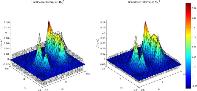
Figure 3: Confidence intervals for Landweber regression and its debiased estimator.

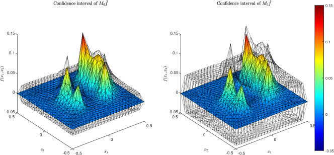
Figure 4: Confidence intervals for SOAR regression and its debiased estimator.

From Figures 3 to 8, as well as 10 (correspondingly, Figures 5 to 8, and 10 in Appendix B), it can be observed that when the general estimators $\hat{f}$ exhibit issues such as overfitting or underfitting in confidence interval sizes, the debiased estimators $\tilde{f}$, which perform well in coverage probability, achieve better results. In contrast, the debiased estimators $\tilde{f}$, which perform poorly in coverage probability, still have little impact on confidence interval size.

7 Conclusion and outlook

In this paper, we introduced a unified framework for designing and analyzing a broad class of linear regression methods, inspired by classical regularization theory. This framework encompasses traditional methods such as least squares and Ridge regression, as well as innovative approaches including Landweber regression (10), Showalter regression (12), SOAR regression (14), HBF regression (17), FAR regression (20), AR^κ regression (21), and Nesterov acceleration regression (22). Building upon this framework, we proposed a novel class of debiased and thresholded regression methods designed to promote feature selection and achieving sparsity.

Our theoretical analysis established the consistency and Gaussian approximation theorems for these new methods. The debiased and thresholded regression methods demonstrated significant advantages over conventional methods, including Lasso, particularly in high-dimensional settings. Extensive numerical simulations confirmed the favorable finite-sample performance of these methods, underscoring their potential in various practical applications where high-dimensional data is prevalent.

The success of our proposed methods lies in their ease of computation via a closed-form expression while effectively addressing high-dimensional challenges. These methods not only provide robust parameter estimates but also enhance model selection by promoting sparsity, making them valuable tools for statisticians and data scientists working with complex datasets.

Future research could explore further extensions of this framework to other types of regression problems and the development of more efficient computational algorithms for handling even larger datasets. Additionally, investigating the performance of these methods in real-world applications across different domains could provide further insights into their practical utility and robustness.

Acknowledgments and Disclosure of Funding

This work was partially supported by the Shenzhen Sci-Tech Fund (Grant No. RCJC20231211090030059), National Natural Science Foundation of China (No. 12171036), National Key Research and Development Program of China (No. 2022YFC3310300) and Beijing Natural Science Foundation (No. Z210001).

Appendix A Proofs

To prove Theorem 3 and the rest of the theorems, we state Lemma 13 (Whittle, 1960, Theorem 2) which directly contributes to the model selection consistency:

Lemma 13.

Suppose random variables $e_{1},\cdots,e_{n}$ are i.i.d., $\mathbb{E}e_{1}=0$, and there exists a constant $m>0$ such that $\mathbb{E}\left|e_{1}\right|^{m}<\infty$. In addition suppose the matrix $\Gamma=\left(\gamma_{ij}\right)_{i=1,2,\cdots,k,j=1,2,\cdots,n}$ satisfies

$$\max_{i=1,2,\cdots,k}\sum_{j=1}^{n}\gamma_{ij}^{2}\leq D,\quad D>0.$$

Then there exists a constant $E$ which only depends on $m$ and $\mathbb{E}\left|e_{1}\right|^{m}$ such that for all $\delta>0$,

$$\mathbb{P}\left(\max_{i=1,2,\cdots,k}\left|\sum_{j=1}^{n}\gamma_{ij}e_{j}\right|>\delta\right)\leq\frac{kED^{m/2}}{\delta^{m}}.$$

In addition, we also need to introduce the thin singular value decomposition of the design matrix $\mathbf{X}_{n}$, as detailed in (Horn and Johnson, 1985, Theorem 7.3.2), as follows:

$$\mathbf{X}_{n}=\mathbf{U}\text{\leavevmode\nobreak\ diag}\{\sqrt{\lambda_{1}},\cdots,\sqrt{\lambda_{s}}\}\mathbf{V}^{\textrm{T}}:=\mathbf{U}\varLambda\mathbf{V}^{\textrm{T}},$$ (49)

where $\left(\mathbf{U},\mathbf{V},\{\sqrt{\lambda_{i}}\}^{s}_{i=1}\right)$ represents the singular system of matrix $\mathbf{X}_{n}$. $0<\lambda_{s}\leq\cdots\leq\lambda_{1}$ are ordered eigenvalues of the square matrix $\mathbf{X}_{n}^{\textrm{T}}\mathbf{X}_{n}$. $\mathbf{U}=[u_{ij}]_{n\times s}$ and $\mathbf{V}=[v_{ij}]_{p\times s}$ in equation (49) are respectively $n\times s$ and $p\times s$ orthonormal matrices, satisfying $\mathbf{U}^{\textrm{T}}\mathbf{U}=\mathbf{V}^{\textrm{T}}\mathbf{V}=\mathbf{I}_{s}$, $\mathbf{I}_{s}$ denotes the $s\times s$ identity matrix. $s\leq\min\{n,p\}$ is the rank of the design matrix $\mathbf{X}_{n}$.

Then we have

$$\hat{\boldsymbol{\beta}}_{\alpha}-\boldsymbol{\beta}=\frac{1}{n}\mathbf{V}g_{\alpha}(\frac{1}{n}\varLambda^{2})\varLambda\mathbf{U}^{\textrm{T}}\boldsymbol{e}_{n}-\mathbf{V}r_{\alpha}(\frac{1}{n}\varLambda^{2})\mathbf{V}^{\textrm{T}}\boldsymbol{\beta},$$ (50)

and

$$\tilde{\boldsymbol{\beta}}_{\alpha}-\boldsymbol{\beta}=\frac{1}{n}\mathbf{V}[I+r_{\alpha}(\frac{1}{n}\varLambda^{2})]g_{\alpha}(\frac{1}{n}\varLambda^{2})\varLambda\mathbf{U}^{\textrm{T}}\boldsymbol{e}_{n}-\mathbf{V}r^{2}_{\alpha}(\frac{1}{n}\varLambda^{2})\mathbf{V}^{\textrm{T}}\boldsymbol{\beta}.$$ (51)

Proof of Theorem 3 Define $\boldsymbol{\zeta}=[\zeta_{1},\cdots,\zeta_{n}]^{\textrm{T}}:=\mathbf{V}^{\textrm{T}}\boldsymbol{\beta}$, then the component-wise error of $\hat{\boldsymbol{\beta}}_{\alpha}$ equals

$$(\hat{\boldsymbol{\beta}}_{\alpha})_{i}-\beta_{i}=\sum_{j=1}^{s}\frac{v_{ij}}{n}g_{\alpha}(\frac{\lambda_{j}}{n})\lambda_{j}^{\frac{1}{2}}\sum_{l=1}^{n}u_{lj}e_{l}-\sum_{j=1}^{s}v_{ij}\zeta_{j}r_{\alpha}\left(\frac{\lambda_{j}}{n}\right).$$

From Cauchy inequality, Definition 2 and (D1-3) of Definition 10, we can deduce that

$$\max_{i=1,2,\cdots,p}\left|\sum_{j=1}^{s}v_{ij}\zeta_{j}r_{\alpha}\left(\frac{\lambda_{j}}{n}\right)\right| \leq\max_{i=1,2,\cdots,p}\sqrt{\sum_{j=1}^{s}v_{ij}^{2}}\sqrt{\sum_{j=1}^{s}\zeta^{2}_{j}r^{2}_{\alpha}\left(\frac{\lambda_{j}}{n}\right)}$$ (52)

$$\leq\frac{C_{*}n^{d}\alpha^{d}}{\lambda^{d}_{s}}\sqrt{\sum_{j=1}^{s}\zeta^{2}_{j}}=O\left(n^{\alpha_{\beta}-d\delta}\right),$$

and

$$\max_{i=1,\cdots,p}\sum_{l=1}^{n}\left(\sum_{j=1}^{s}\frac{v_{ij}}{n}g_{\alpha}(\frac{\lambda_{j}}{n})\lambda_{j}^{\frac{1}{2}}u_{lj}\right)^{2}=\max_{i=1,\cdots,p}\sum_{j=1}^{s}\frac{v_{ij}^{2}}{n^{2}}g^{2}_{\alpha}(\frac{\lambda_{j}}{n})\lambda_{j}\leq\max_{i=1,\cdots,p}\sum_{j=1}^{s}\frac{4v_{ij}^{2}}{\lambda_{j}}\leq\frac{4}{\lambda_{s}}.$$ (53)

Further, we can obtain

$$\mathbb{P}\left(\max_{i=1,2,\cdots,p}\left|\sum_{j=1}^{s}\frac{v_{ij}}{n}g_{\alpha}(\frac{\lambda_{j}}{n})\lambda_{j}^{\frac{1}{2}}\sum_{l=1}^{n}u_{lj}e_{l}\right|>\delta\right)\leq\frac{pE2^{m}}{\lambda_{s}^{\frac{m}{2}}\delta^{m}}\text{ for any }\ \delta>0,$$ (54)

where $E$ is the constant defined in Lemma 13. Subsequently, (54) implied that

$$\max_{i=1,2,\cdots,p}\left|\sum_{k=1}^{s}\frac{v_{ij}}{n}g_{\alpha}(\frac{\lambda_{j}}{n})\lambda_{j}^{\frac{1}{2}}\sum_{l=1}^{n}u_{lk}e_{l}\right|=O_{p}\left(n^{\frac{\alpha_{p}}{m}-\eta}\right).$$

which yields (26).

By using a similar proof approach, we can derive the following results.

$$(\tilde{\boldsymbol{\beta}}_{\alpha})_{i}-\beta_{i}=\sum_{j=1}^{s}\frac{v_{ij}}{n}[1+r_{\alpha}(\frac{\lambda_{j}}{n})]g_{\alpha}(\frac{\lambda_{j}}{n})\lambda_{j}^{\frac{1}{2}}\sum_{l=1}^{n}u_{lj}e_{l}-\sum_{j=1}^{s}v_{ij}\zeta_{j}r^{2}_{\alpha}\left(\frac{\lambda_{j}}{n}\right),$$ (55)

$$\max_{i=1,,\cdots,p}\left|\sum_{j=1}^{s}v_{ij}\zeta_{j}r^{2}_{\alpha}\left(\frac{\lambda_{j}}{n}\right)\right|\leq\max_{i=1,2,\cdots,p}\sqrt{\sum_{j=1}^{s}v_{ij}^{2}}\sqrt{\sum_{j=1}^{s}\zeta^{2}_{j}r^{2}_{\alpha}\left(\frac{\lambda_{j}}{n}\right)}=O\left(n^{\alpha_{\beta}-2d\delta}\right),$$ (56)

and

$$\max_{i=1,2,\cdots,p}\sum_{l=1}^{n}\left(\sum_{j=1}^{s}\frac{v_{ij}}{n}[1+r_{\alpha}(\frac{\lambda_{j}}{n})]g_{\alpha}(\frac{\lambda_{j}}{n})\lambda^{\frac{1}{2}}_{j}u_{lj}\right)^{2}\leq\frac{16}{\lambda_{s}}.$$ (57)

By combining (55)-(57) with Lemma 13, we can derive the estimate (27).  

Proof of Theorem 4 From (50),

$$\mathbb{P}\left(\widehat{\mathcal{N}}_{b_{n}}\neq\mathcal{N}_{b_{n}}\right)$$

$$\leq\mathbb{P}\left(\min_{i\in\mathcal{N}_{b_{n}}}\left|\hat{\theta}_{i}\right|\leq b_{n}\right)+\mathbb{P}\left(\max_{i\notin\mathcal{N}_{b_{n}}}\left|\hat{\theta}_{i}\right|>b_{n}\right)$$

$$\leq\mathbb{P}\left(\min_{i\in\mathcal{N}_{b_{n}}}\left|\beta_{i}\right|-\max_{i\in\mathcal{N}_{b_{n}}}\left|\sum_{j=1}^{s}v_{ij}\zeta_{j}r_{\alpha}\left(\frac{\lambda_{j}}{n}\right)\right|-\max_{i\in\mathcal{N}_{b_{n}}}\left|\sum_{j=1}^{s}\frac{v_{ij}}{n}g_{\alpha}(\frac{\lambda_{j}}{n})\lambda_{j}^{\frac{1}{2}}\sum_{l=1}^{n}u_{lj}e_{l}\right|\leq b_{n}\right)$$

$$\quad+\mathbb{P}\left(\max_{i\notin\mathcal{N}_{b_{n}}}\left|\beta_{i}\right|+\max_{i\notin\mathcal{N}_{b_{n}}}\left|\sum_{j=1}^{s}v_{ij}\zeta_{j}r_{\alpha}\left(\frac{\lambda_{j}}{n}\right)\right|+\max_{i\notin\mathcal{N}_{b_{n}}}\left|\sum_{j=1}^{s}\frac{v_{ij}}{n}g_{\alpha}(\frac{\lambda_{j}}{n})\lambda_{j}^{\frac{1}{2}}\sum_{l=1}^{n}u_{lj}e_{l}\right|>b_{n}\right).$$

Furthermore, for sufficiently large $n$, from (53), Assumption 4 and (D1-1) of Definition 1 we have

$$\min_{i\in\mathcal{N}_{b_{n}}}\left|\theta_{i}\right|-\max_{i\in\mathcal{N}_{b_{n}}}\left|\sum_{j=1}^{s}v_{ij}\zeta_{j}r_{\alpha}\left(\frac{\lambda_{j}}{n}\right)\right|-b_{n} >\frac{1}{2}\left(\frac{1}{c_{b}}-1\right)b_{n},$$

$$b_{n}-\max_{i\notin\mathcal{N}_{b_{n}}}\left|\theta_{i}\right|-\max_{i\notin\mathcal{N}_{b_{n}}}\left|\sum_{j=1}^{s}v_{ij}\zeta_{j}r_{\alpha}\left(\frac{\lambda_{j}}{n}\right)\right| >\frac{1}{2}\left(1-c_{b}\right)b_{n}.$$

Drawing from Lemma 13, we infer the inequality

$$\mathbb{P}\left(\widehat{\mathcal{N}}_{b_{n}}\neq\mathcal{N}_{b_{n}}\right)\leq\frac{E2^{m}\left|\mathcal{N}_{b_{n}}\right|}{\lambda_{s}^{\frac{m}{2}}\left(\frac{1}{2}\left(\frac{1}{c_{b}}-1\right)b_{n}\right)^{m}}+\frac{E2^{m}\left(p-\left|\mathcal{N}_{b_{n}}\right|\right)}{\lambda_{s}^{\frac{m}{2}}\left(\frac{1}{2}\left(1-c_{b}\right)b_{n}\right)^{m}}=O\left(n^{\alpha_{p}+m\nu_{b}-m\eta}\right).$$

which yields (28).

In a closely analogous manner, we can obtain

$$\mathbb{P}\left(\widetilde{\mathcal{N}}_{b_{n}}\neq\mathcal{N}_{b_{n}}\right)$$

$$\leq\mathbb{P}\left(\min_{i\in\mathcal{N}_{b_{n}}}\left|\hat{\theta}_{i}\right|\leq b_{n}\right)+\mathbb{P}\left(\max_{i\notin\mathcal{N}_{b_{n}}}\left|\hat{\theta}_{i}\right|>b_{n}\right)$$

$$\leq\mathbb{P}\left(\min_{i\in\mathcal{N}_{b_{n}}}\left|\beta_{i}\right|-\max_{i\in\mathcal{N}_{b_{n}}}\left|\sum_{j=1}^{s}v_{ij}\zeta_{j}r^{2}_{\alpha}\left(\frac{\lambda_{j}}{n}\right)\right|\right.$$

$$\qquad\left.-\max_{i\in\mathcal{N}_{b_{n}}}\left|\sum_{j=1}^{s}\frac{v_{ij}}{n}[1+r_{\alpha}(\frac{\lambda_{j}}{n})]g_{\alpha}(\frac{\lambda_{j}}{n})\lambda^{\frac{1}{2}}_{j}\sum_{l=1}^{n}u_{lj}e_{l}\right|\leq b_{n}\right)$$

$$\quad+\mathbb{P}\left(\max_{i\notin\mathcal{N}_{b_{n}}}\left|\beta_{i}\right|+\max_{i\notin\mathcal{N}_{b_{n}}}\left|\sum_{j=1}^{s}v_{ij}\zeta_{j}r^{2}_{\alpha}\left(\frac{\lambda_{j}}{n}\right)\right|\right.$$

$$\qquad\left.+\max_{i\notin\mathcal{N}_{b_{n}}}\left|\sum_{j=1}^{s}\frac{v_{ij}}{n}[1+r_{\alpha}(\frac{\lambda_{j}}{n})]g_{\alpha}(\frac{\lambda_{j}}{n})\lambda^{\frac{1}{2}}_{j}\sum_{l=1}^{n}u_{lj}e_{l}\right|>b_{n}\right).$$

which yields (29) by using (56), (53) and Lemma 13.  

Proof of Theorem 5 According to Theorem 4, we only need to consider the case when $\widehat{\mathcal{N}}_{b_{n}}=\mathcal{N}_{b_{n}}$. As stated in Assumption 4, we have

$$\left\lVert\hat{\boldsymbol{\theta}}-\boldsymbol{\beta}\right\rVert^{2}_{2}$$

$$=\sum_{i\in\mathcal{N}_{b_{n}}}\left(\hat{\theta}_{i}-\beta_{i}\right)^{2}+\sum_{i\notin\mathcal{N}_{b_{n}}}\beta_{i}^{2}$$

$$\leq 2\sum_{i\in\mathcal{N}_{b_{n}}}\left(\sum_{j=1}^{s}v_{ij}\zeta_{j}r_{\alpha}\left(\frac{\lambda_{j}}{n}\right)\right)^{2}+2\sum_{i\in\mathcal{N}_{b_{n}}}\left(\sum_{j=1}^{s}\frac{v_{ij}}{n}g_{\alpha}(\frac{\lambda_{j}}{n})\lambda_{j}^{\frac{1}{2}}\sum_{l=1}^{n}u_{lj}e_{l}\right)^{2}+\sum_{i\notin\mathcal{N}_{b_{n}}}\beta_{i}^{2}$$

$$\leq 2\sum_{i\in\mathcal{N}_{b_{n}}}\left(\sum_{j=1}^{s}v_{ij}\zeta_{j}r_{\alpha}\left(\frac{\lambda_{j}}{n}\right)\right)^{2}+2\sum_{i\in\mathcal{N}_{b_{n}}}\left(\sum_{j=1}^{s}\frac{v_{ij}}{n}g_{\alpha}(\frac{\lambda_{j}}{n})\lambda_{j}^{\frac{1}{2}}\sum_{l=1}^{n}u_{lj}e_{l}\right)^{2}$$

$$\quad+C_{b}c_{b}n^{-v_{b}}\sum_{i\notin\mathcal{N}_{b_{n}}}\left|\beta_{i}\right|$$

$$\leq 2\left|\mathcal{N}_{b_{n}}\right|\left[\max_{i=1,2,\cdots,p}\left(\sum_{j=1}^{s}v_{ij}\zeta_{j}r_{\alpha}\left(\frac{\lambda_{j}}{n}\right)\right)^{2}+\max_{i=1,2,\cdots,p}\left(\sum_{j=1}^{s}\frac{v_{ij}}{n}g_{\alpha}(\frac{\lambda_{j}}{n})\lambda_{j}^{\frac{1}{2}}\sum_{l=1}^{n}u_{lj}e_{l}\right)^{2}\right]$$

$$\quad+C_{b}c_{b}n^{-v_{b}}\sum_{i\notin\mathcal{N}_{b_{n}}}\left|\beta_{i}\right|.$$

According to the inequality (52) and Assumptions 1 and 5 we obtain

$$\left|\mathcal{N}_{b_{n}}\right|\times\max_{i=1,2,\cdots,p}\left(\sum_{j=1}^{s}v_{ij}\zeta_{j}r_{\alpha}\left(\frac{\lambda_{j}}{n}\right)\right)^{2}=O\left(n^{2\alpha_{\beta}+2\eta-2d\delta-2\alpha_{\sigma}}\right).$$

For the second term, the inequality (54) implies that

$$\max_{i=1,2,\cdots,p}\left|\sum_{k=1}^{s}\frac{v_{ij}}{n}g_{\alpha}(\frac{\lambda_{j}}{n})\lambda_{j}^{\frac{1}{2}}\sum_{l=1}^{n}u_{lk}e_{l}\right|=O_{p}\left(n^{\frac{\alpha_{p}}{m}-\eta}\right).$$

Building on this result, we conclude

$$\left|\mathcal{N}_{b_{n}}\right|\times\max_{i=1,2,\cdots,p}\left(\sum_{k=1}^{s}\frac{v_{ij}}{n}g_{\alpha}(\frac{\lambda_{j}}{n})\lambda_{j}^{\frac{1}{2}}\sum_{l=1}^{n}u_{lk}e_{l}\right)^{2}=O_{p}\left(n^{\frac{2\alpha_{p}}{m}-2\alpha_{\sigma}}\right).$$

In conjunction with Assumptions 4, 5 and Definition 2, above analysis supports a further conclusion that the 2-norm difference between the estimator $\hat{\boldsymbol{\theta}}$ and the true parameter $\boldsymbol{\beta}$ has the asymptotical estimate for $d>\frac{\alpha_{\beta}+\eta-\frac{\alpha_{p}}{m}}{\delta}$:

$$\left\lVert\hat{\boldsymbol{\theta}}-\boldsymbol{\beta}\right\rVert_{2}=O_{p}\left(n^{\frac{\alpha_{p}}{m}-\alpha_{\sigma}}\right).$$

In the same vein, it is sufficient to consider the case when $\widetilde{\mathcal{N}}_{b_{n}}=\mathcal{N}_{b_{n}}$ according to Theorem 4.

$$\left\lVert\tilde{\boldsymbol{\theta}}-\boldsymbol{\beta}\right\rVert^{2}_{2}$$

$$=\sum_{i\in\mathcal{N}_{b_{n}}}\left(\tilde{\theta}_{i}-\beta_{i}\right)^{2}+\sum_{i\notin\mathcal{N}_{b_{n}}}\beta_{i}^{2}$$

$$\leq 2\sum_{i\in\mathcal{N}_{b_{n}}}\left(\sum_{j=1}^{s}v_{ij}\zeta_{j}r^{2}_{\alpha}\left(\frac{\lambda_{j}}{n}\right)\right)^{2}+2\sum_{i\in\mathcal{N}_{b_{n}}}\left(\sum_{j=1}^{s}\frac{v_{ij}}{n}[1+r_{\alpha}(\frac{\lambda_{j}}{n})]g_{\alpha}(\frac{\lambda_{j}}{n})\lambda_{j}^{\frac{1}{2}}\sum_{l=1}^{n}u_{lj}e_{l}\right)^{2}+\sum_{i\notin\mathcal{N}_{b_{n}}}\beta_{i}^{2}$$

$$\leq 2\left|\mathcal{N}_{b_{n}}\right|\left[\max_{i=1,2,\cdots,p}\left(\sum_{j=1}^{s}v_{ij}\zeta_{j}r^{2}_{\alpha}\left(\frac{\lambda_{j}}{n}\right)\right)^{2}+\max_{i=1,2,\cdots,p}\left(\sum_{j=1}^{s}\frac{v_{ij}}{n}[1+r_{\alpha}(\frac{\lambda_{j}}{n})]g_{\alpha}(\frac{\lambda_{j}}{n})\lambda_{j}^{\frac{1}{2}}\sum_{l=1}^{n}u_{lj}e_{l}\right)^{2}\right]$$

$$\quad+C_{b}c_{b}n^{-v_{b}}\sum_{i\notin\mathcal{N}_{b_{n}}}\left|\beta_{i}\right|.$$

From (57), we have

$$\mathbb{P}\left(\max_{i=1,2,\cdots,p}\left|\sum_{j=1}^{s}\frac{v_{ij}}{n}[1+r_{\alpha}(\frac{\lambda_{j}}{n})]g_{\alpha}(\frac{\lambda_{j}}{n})\lambda^{\frac{1}{2}}_{j}\sum_{l=1}^{n}u_{lj}e_{l}\right|>\delta\right)\leq\frac{pE4^{m}}{\lambda_{s}^{\frac{m}{2}}\delta^{m}}\text{ for all }\delta>0.$$

Here $E$ is the constant defined in Lemma 13. Furthermore, we can find that

$$\left|\mathcal{N}_{b_{n}}\right|\times\max_{i=1,2,\cdots,p}\left(\sum_{k=1}^{s}\frac{v_{ij}}{n}[1+r_{\alpha}(\frac{\lambda_{j}}{n})]g_{\alpha}(\frac{\lambda_{j}}{n})\lambda_{j}^{\frac{1}{2}}\sum_{l=1}^{n}u_{lk}e_{l}\right)^{2}=O_{p}\left(n^{\frac{2\alpha_{p}}{m}-2\alpha_{\sigma}}\right).$$

By combining with Assumption 4, 5, Remark 2 and (56), we prove (31).  

Proof of Theorem 6 As mentioned above, we only need to consider the situation when $\widehat{\mathcal{N}}_{b_{n}}=\mathcal{N}_{b_{n}}$. In this case, we have the error decomposition:

$$\widehat{\sigma}^{2}-\sigma^{2}= \frac{1}{n}\sum_{i=1}^{n}\left(e_{i}-\sum_{j\in\mathcal{N}_{b_{n}}}x_{ij}\left(\hat{\theta}_{j}-\beta_{j}\right)+\sum_{j\notin\mathcal{N}_{b_{n}}}x_{ij}\beta_{j}\right)^{2}-\sigma^{2}$$ (58)

$$= \frac{1}{n}\sum_{i=1}^{n}e_{i}^{2}-\sigma^{2}+\frac{1}{n}\sum_{i=1}^{n}\left(\sum_{j\in\mathcal{N}_{b_{n}}}x_{ij}\left(\hat{\theta}_{j}-\beta_{j}\right)\right)^{2}+\frac{1}{n}\sum_{i=1}^{n}\left(\sum_{j\notin\mathcal{N}_{b_{n}}}x_{ij}\beta_{j}\right)^{2}$$

$$-\frac{2}{n}\sum_{i=1}^{n}\sum_{j\in\mathcal{N}_{b_{n}}}e_{i}x_{ij}\left(\hat{\theta}_{j}-\beta_{j}\right)+\frac{2}{n}\sum_{i=1}^{n}\sum_{j\notin\mathcal{N}_{b_{n}}}e_{i}x_{ij}\beta_{j}$$

$$-\frac{2}{n}\sum_{i=1}^{n}\left(\sum_{j\in\mathcal{N}_{b_{n}}}x_{ij}\left(\hat{\theta}_{j}-\beta_{j}\right)\right)\left(\sum_{j\notin\mathcal{N}_{b_{n}}}x_{ij}\beta_{j}\right).$$

Now, let us estimate the right-hand side of the error decomposition (58) term by term.

From Assumption 3, Lemma 13 and the inequality $\mathbb{E}\left(\frac{1}{n}\sum\limits_{i=1}^{n}e_{i}^{2}-\sigma^{2}\right)^{2}\leq\frac{2}{n}\left(\mathbb{E}e_{1}^{4}+\sigma^{4}\right)=O(\frac{1}{n})$, we obtain the estimation of the first term in (58):

$$\frac{1}{n}\sum\limits_{i=1}^{n}e_{i}^{2}-\sigma^{2}=O_{p}(\frac{1}{\sqrt{n}}).$$

For the second term in the error decomposition (58), from Assumption 1 and (52), we derive that

$$\frac{1}{n}\sum_{i=1}^{n} \left(\sum_{j\in\mathcal{N}_{b_{n}}}x_{ij}\left(\hat{\theta}_{j}-\beta_{j}\right)\right)^{2}$$ (59)

$$\leq C_{\lambda}\sum_{j\in\mathcal{N}_{b_{n}}}\left(\hat{\theta}_{j}-\beta_{j}\right)^{2}$$

$$\leq 2C_{\lambda}\sum_{j\in\mathcal{N}_{b_{n}}}\left[\left(\sum_{k=1}^{s}v_{jk}\zeta_{j}r_{\alpha}\left(\frac{\lambda_{k}}{n}\right)\right)^{2}+\left(\sum_{k=1}^{s}\frac{1}{n}v_{jk}g_{\alpha}(\frac{\lambda_{k}}{n})\sqrt{\lambda_{k}}\sum_{l=1}^{n}u_{lk}e_{l}\right)^{2}\right]$$

$$=O\left(n^{2\alpha_{\beta}-2d\delta}\left|\mathcal{N}_{b_{n}}\right|\right)+2C_{\lambda}\sum_{j\in\mathcal{N}_{b_{n}}}\left(\sum_{k=1}^{s}\frac{1}{n}v_{jk}g_{\alpha}(\frac{\lambda_{k}}{n})\sqrt{\lambda_{k}}\sum_{l=1}^{n}u_{lk}e_{l}\right)^{2}.$$

Since

$$\mathbb{E}\sum_{j\in\mathcal{N}_{b_{n}}}\left(\sum_{k=1}^{s}\frac{1}{n}q_{ik}g_{\alpha}(\frac{\lambda_{k}}{n})\sqrt{\lambda_{k}}\sum_{l=1}^{n}u_{lk}e_{l}\right)^{2} =\sigma^{2}\sum_{j\in\mathcal{N}_{b_{n}}}\sum_{l=1}^{n}\left(\sum_{k=1}^{s}\frac{1}{n}q_{ik}g_{\alpha}(\frac{\lambda_{k}}{n})\sqrt{\lambda_{k}}u_{lk}\right)^{2}$$

$$=\sigma^{2}\sum_{j\in\mathcal{N}_{b_{n}}}\sum_{k=1}^{s}\frac{1}{n^{2}}q^{2}_{ik}g^{2}_{\alpha}(\frac{\lambda_{k}}{n})\lambda_{k}$$

$$\leq\frac{4\sigma^{2}\left|\mathcal{N}_{b_{n}}\right|}{\lambda_{s}},$$

we have

$$\frac{1}{n}\sum\limits_{i=1}^{n}\left(\sum\limits_{j\in\mathcal{N}_{b_{n}}}x_{ij}\left(\hat{\theta}_{j}-\beta_{j}\right)\right)^{2}=O_{p}\left(n^{2\alpha_{\beta}-2d\delta}\left|\mathcal{N}_{b_{n}}\right|+n^{-2\eta}\left|\mathcal{N}_{b_{n}}\right|\right).$$

For the third term in (58), from Assumption 5 we have

$$\frac{1}{n}\sum_{i=1}^{n}\left(\sum_{j\notin\mathcal{N}_{b_{n}}}x_{ij}\beta_{j}\right)^{2}\leq C_{\lambda}\sum_{j\notin\mathcal{N}_{b_{n}}}\beta_{j}^{2}\leq C_{\lambda}b_{n}\sum_{j\notin\mathcal{N}_{b_{n}}}\left|\beta_{j}\right|=O\left(n^{-\alpha_{\sigma}}\right).$$ (60)

For the fourth term in (58), from Cauchy inequality and inequality (59), we have

$$\mathbb{E}\frac{1}{n}\left|\sum_{i=1}^{n}\sum_{j\in\mathcal{N}_{b_{n}}}e_{i}x_{ij}\left(\hat{\theta}_{j}-\beta_{j}\right)\right|\leq \frac{1}{n}\mathbb{E}\sqrt{\sum_{i=1}^{n}e_{i}^{2}}\sqrt{\sum_{i=1}^{n}\left(\sum_{j\in\mathcal{N}_{b_{n}}}x_{ij}\left(\hat{\theta}_{j}-\beta_{j}\right)\right)^{2}}$$

$$\leq \sqrt{\frac{\mathbb{E}\sum\limits_{i=1}^{n}e_{i}^{2}}{n}}\sqrt{\frac{1}{n}\mathbb{E}\sum_{i=1}^{n}\left(\sum_{j\in\mathcal{N}_{b_{n}}}x_{ij}\left(\hat{\theta}_{j}-\beta_{j}\right)\right)^{2}}$$

$$= O\left(\sqrt{\left.n^{2\alpha_{\beta}-2d\delta}\left|\mathcal{N}_{b_{n}}\right|+n^{-2\eta}\left|\mathcal{N}_{b_{n}}\right|\right)}\right).$$

It is sufficiently to illustrates that

$$\frac{1}{n}\left|\sum_{i=1}^{n}\sum_{j\in\mathcal{N}_{b_{n}}}e_{i}x_{ij}\left(\hat{\theta}_{j}-\beta_{j}\right)\right|=O_{p}\left(n^{\alpha_{\beta}-d\delta}\sqrt{\left|\mathcal{N}_{b_{n}}\right|}+n^{-\eta}\sqrt{\left|\mathcal{N}_{b_{n}}\right|}\right).$$

In reference to (59) and (60), and employing the Cauchy-Schwarz inequality, we ascertain the asymptotic order of the fifth term as (61)

$$\frac{1}{n}\sum_{i=1}^{n}\sum_{j\notin\mathcal{N}_{b_{n}}}e_{i}x_{ij}\beta_{j}=O_{p}\left(n^{-\left(1+\alpha_{\sigma}\right)/2}\right)$$ (61)

by using

$$\mathbb{E}\left|\frac{1}{n}\sum_{i=1}^{n}\sum_{j\notin\mathcal{N}_{b_{n}}}e_{i}x_{ij}\beta_{j}\right|^{2}=\frac{\sigma^{2}}{n^{2}}\sum_{i=1}^{n}\left(\sum_{j\notin\mathcal{N}_{b_{n}}}x_{ij}\beta_{j}\right)^{2}\leq\frac{\sigma^{2}C_{\lambda}}{n}\sum_{j\notin\mathcal{N}_{b_{n}}}\beta_{j}^{2}.$$

Then, the convergence order for the last term is

$$\frac{1}{n}\left|\sum_{i=1}^{n}\left(\sum_{j\in\mathcal{N}_{b_{n}}}x_{ij}\left(\hat{\theta}_{j}-\beta_{j}\right)\right)\left(\sum_{j\notin\mathcal{N}_{b_{n}}}x_{ij}\beta_{j}\right)\right|$$

$$\leq C_{\lambda}\sqrt{\sum_{j\in\mathcal{N}_{b_{n}}}\left(\hat{\theta}_{j}-\beta_{j}\right)^{2}}\sqrt{\sum_{j\notin\mathcal{N}_{b_{n}}}\beta_{j}^{2}}=O_{p}\left(n^{\alpha_{\beta}-d\delta-\alpha_{\sigma}/2}\sqrt{\left|\mathcal{N}_{b_{n}}\right|}+n^{-\eta-\alpha_{\sigma}/2}\sqrt{\left|\mathcal{N}_{b_{n}}\right|}\right).$$

From the the estimation (28) in Theorem 4, $\mathbb{P}\left(\widehat{\mathcal{N}}_{b_{n}}\neq\mathcal{N}_{b_{n}}\right)\to 0$ as $n\to\infty$.

Hence, we conclude that

$$\left|\widehat{\sigma}^{2}-\sigma^{2}\right|=O_{p}\left(\frac{1}{\sqrt{n}}+n^{\alpha_{\beta}-d\delta}\sqrt{\left|\mathcal{N}_{b_{n}}\right|}+n^{-\eta}\sqrt{\left|\mathcal{N}_{b_{n}}\right|}+n^{-\alpha_{\sigma}}\right).$$

Finally, the theorem holds according to Assumption 2 and 5.

Similarly, let $\widetilde{\mathcal{N}}_{b_{n}}=\mathcal{N}_{b_{n}}$. From the arguments presented in the proof of Theorem 6, it follows that

$$\widehat{\sigma}^{2}-\sigma^{2}= \frac{1}{n}\sum_{i=1}^{n}\left(e_{i}-\sum_{j\in\mathcal{N}_{b_{n}}}x_{ij}\left(\tilde{\theta}_{j}-\beta_{j}\right)+\sum_{j\notin\mathcal{N}_{b_{n}}}x_{ij}\theta_{j}\right)^{2}-\sigma^{2}$$

$$= \frac{1}{n}\sum_{i=1}^{n}e_{i}^{2}-\sigma^{2}+\frac{1}{n}\sum_{i=1}^{n}\left(\sum_{j\in\mathcal{N}_{b_{n}}}x_{ij}\left(\tilde{\theta}_{j}-\theta_{j}\right)\right)^{2}+\frac{1}{n}\sum_{i=1}^{n}\left(\sum_{j\notin\mathcal{N}_{b_{n}}}x_{ij}\theta_{j}\right)^{n}$$

$$-\frac{2}{n}\sum_{i=1}^{n}\sum_{j\in\mathcal{N}_{b_{n}}}e_{i}x_{ij}\left(\tilde{\theta}_{j}-\theta_{j}\right)+\frac{2}{n}\sum_{i=1}^{n}\sum_{j\notin\mathcal{N}_{b_{n}}}e_{i}x_{ij}\theta_{j}$$

$$-\frac{2}{n}\sum_{i=1}^{n}\left(\sum_{j\in\mathcal{N}_{b_{n}}}x_{ij}\left(\tilde{\theta}_{j}-\theta_{j}\right)\right)\left(\sum_{j\notin\mathcal{N}_{b_{n}}}x_{ij}\theta_{j}\right)$$

$$= O_{p}\left(\frac{1}{\sqrt{n}}+n^{\alpha_{\beta}-2d\delta}\sqrt{\left|\mathcal{N}_{b_{n}}\right|}+n^{-\eta}\sqrt{\left|\mathcal{N}_{b_{n}}\right|}+n^{-\alpha_{\sigma}}\right)$$

$$= O_{p}\left(n^{-\alpha_{\sigma}}\right),$$

which yields the required estimate.  

Before proving the asymptotic normality of our estimator, we need two lemmas from Chernozhukov et al. (2013), which use a joint normal distribution to approximate the distribution of linear combinations of independent random variables.

Lemma 14.

Suppose $\boldsymbol{e}_{n}=\left(e_{1},\cdots,e_{n}\right)^{\textrm{T}}$ are joint normal random variables with mean $\mathbb{E}\boldsymbol{e}_{n}=\boldsymbol{0}$, non-singular covariance matrix $\mathbb{E}\boldsymbol{e}_{n}\boldsymbol{e}_{n}^{\textrm{T}}$, and positive marginal variance $\sigma_{i}^{2}=\mathbb{E}e_{i}^{2}>$ $0,i=1,2,\cdots,n$. In addition, suppose there exists two constants $0<c_{0}\leq C_{0}<\infty$ such that $c_{0}\leq\sigma_{i}\leq$ $C_{0}$ for $i=1,2,\cdots,n$. Then for any given $\delta>0$, we have

$$\sup_{x\in\mathbf{R}}\left(\mathbb{P}\left(\max_{i=1,2,\cdots,n}\left|e_{i}\right|\leq x+\delta\right)-\mathbb{P}\left(\max_{i=1,2,\cdots,n}\left|e_{i}\right|\leq x\right)\right)\leq C\delta(\sqrt{\log(n)}+\sqrt{|\log(\delta)|}+1),$$

where the constant $C$ only depends on $c_{0}$ and $C_{0}$.

Lemma 15.

Suppose $\boldsymbol{e}_{n}=\left(e_{1},\cdots,e_{n}\right)^{\textrm{T}}$ are i.i.d. random variables with $\mathbb{E}e_{1}=\boldsymbol{0},\mathbb{E}e_{1}^{2}=$ $\sigma^{2}$ and $\mathbb{E}\left|e_{1}\right|^{3}<\infty$. $\Gamma=\left(\gamma_{ij}\right)_{i=1,2,\cdots,n,j=1,2,\cdots,k}$ is an $n\times k\;(1\leq k\leq n)$ rank $k$ matrix. And there exists constants $0<c_{\Gamma}\leq C_{\Gamma}<\infty$ such that $c_{\Gamma}^{2}\leq\sum_{j=1}^{n}\gamma_{ji}^{2}\leq C_{\Gamma}^{2}$ for $i=1,2,\cdots,k$. $\widehat{\sigma}^{2}=\widehat{\sigma}^{2}(e)$ is an estimator of $\sigma^{2}$, and the random variables $\boldsymbol{e}_{n}^{*}=\left(e_{1}^{*},\cdots,e_{n}^{*}\right)^{\textrm{T}}$, conditional on $\boldsymbol{e}$, are i.i.d. with $e_{1}^{*}$ following a normal distribution $\mathcal{N}\left(0,\widehat{\sigma}^{2}\right)$. Furthermore, $\frac{e_{i}^{*}}{\widehat{\sigma}}$ is independent of $\boldsymbol{e}_{n}$ for $i=1,2,\cdots,n$. In addition, suppose one of the following conditions:

1. there exists a constant $0<\alpha_{\sigma}\leq 1/2$ such that for $j=1,2,\cdots,n,i=1,2,\cdots,k$,

   $$\left|\sigma^{2}-\widehat{\sigma}^{2}\right|=O_{p}\left(n^{-\alpha_{\sigma}}\right),\;\max_{i,j}\left|\gamma_{ji}\right|=o\left(\min\left(n^{\left(\alpha_{\sigma}-1\right)/2}\times\log^{-3/2}(n),n^{-1/3}\times\log^{-3/2}(n)\right)\right.,$$

2. There exists a constant $0<\alpha_{\sigma}<1/2$ such that for $j=1,2,\cdots,n,i=1,2,\cdots,k$,

   $$\left|\sigma^{2}-\widehat{\sigma}^{2}\right|=O_{p}\left(n^{-\alpha_{\sigma}}\right),\;k=o\left(n^{\alpha_{\sigma}}\times\log^{-3}(n)\right),\;\max_{i,j}\left|\gamma_{ji}\right|=O\left(n^{-\alpha_{\sigma}}\times\log^{-3/2}(n)\right),$$

we have

$$\sup_{x\in[0,\infty)}\left|\mathbb{P}\left(\max_{i=1,2,\cdots,k}\left|\sum_{j=1}^{n}\gamma_{ji}e_{j}\right|\leq x\right)-\mathbb{P}^{*}\left(\max_{i=1,2,\cdots,k}\left|\sum_{j=1}^{n}\gamma_{ji}e_{j}^{*}\right|\leq x\right)\right|=o_{p}(1)$$

where $\mathbb{P}^{*}(\cdot)$ represent the conditional probability $\mathbb{P}(\cdot|\mathbf{Y}_{n}))$

In particular, if $\widehat{\sigma}=\sigma$, by assuming one of the following conditions,

1. $$\max_{j=1,2,\cdots,n,i=1,2,\cdots,k}\left|\gamma_{ji}\right|=o\left(n^{-1/3}\times\log^{-3/2}(n)\right),$$

2. $$k\times\max_{j=1,2,\cdots,n,i=1,2,\cdots,k}\left|\gamma_{ji}\right|=o\left(\log^{-9/2}(n)\right),$$

then we have

$$\sup_{x\in[0,\infty)}\left|\mathbb{P}\left(\max_{i=1,2,\cdots,k}\left|\sum_{j=1}^{n}\gamma_{ji}e_{j}\right|\leq x\right)-\mathbb{P}\left(\max_{i=1,2,\cdots,k}\left|\sum_{j=1}^{n}\gamma_{ji}e_{j}^{*}\right|\leq x\right)\right|=o(1).$$

Proof of Theorem 7 Based on (D1-1) of Definition 1, for sufficiently large $n$,

$$\frac{\lambda^{2}r^{2}_{\alpha}(\lambda)}{\alpha^{2}}\leq C_{*}^{2}(2)\leq 4C_{*}^{2}(2)\left[1-r^{2}_{\alpha}(\lambda)\right]^{2}=4C_{*}^{2}(2)\left[1+r_{\alpha}(\lambda)\right]^{2}g^{2}_{\alpha}(\lambda)\lambda^{2}.$$ (62)

From (62), Cauchy inequality and Assumption 2, suppose $\delta=\frac{\eta+\alpha_{\beta}+\delta_{1}}{d}$ with $\delta_{1}>0$. For $i=1,\cdots,p$,

$$\left|\sum_{k=1}^{s}v_{ik}\zeta_{k}r^{2}_{\alpha}\left(\frac{\lambda_{k}}{n}\right)\right| \leq\sqrt{\sum_{k=1}^{s}\frac{v_{ik}^{2}\lambda_{k}}{n^{2}\alpha^{2}}r^{2}_{\alpha}\left(\frac{\lambda_{k}}{n}\right)}\sqrt{\sum_{k=1}^{s}\frac{n^{2}\alpha^{2}\zeta_{k}^{2}r^{2}_{\alpha}\left(\frac{\lambda_{k}}{n}\right)}{\lambda_{k}}}$$

$$\leq\frac{2C_{*}(2)C_{*}(d)\tau_{i}(n\alpha)^{d+1}\|\boldsymbol{\beta}\|_{2}}{\lambda_{s}^{\frac{2d+1}{2}}},$$

and then

$$\max_{i=1,\cdots,p}\frac{1}{\tau_{i}}\left|\sum_{k=1}^{s}v_{ik}\zeta_{k}r^{2}_{\alpha}\left(\frac{\lambda_{k}}{n}\right)\right|=O\left(n^{-\delta_{1}-\delta}\right).$$

Define $t_{il}=\frac{1}{\tau_{i}}\sum\limits_{k=1}^{s}\frac{v_{ik}}{n}u_{lk}[1+r_{\alpha}(\frac{\lambda_{k}}{n})]g_{\alpha}(\frac{\lambda_{k}}{n})\sqrt{\lambda_{k}}$ for $i=1,\cdots,p$ and $l=1,2,\cdots,n$, then (51) implies

$$\max_{i=1,2,\cdots,p}\left|(\tilde{\boldsymbol{\beta}}_{\alpha})_{i}-\beta_{i}\right|= \max_{i=1,2,\cdots,p}\left|\sum_{k=1}^{s}\frac{v_{ik}}{n}[1+r_{\alpha}(\frac{\lambda_{k}}{n})]g_{\alpha}(\frac{\lambda_{k}}{n})\lambda^{\frac{1}{2}}_{k}\sum_{l=1}^{n}u_{lk}e_{l}-\sum_{k=1}^{s}v_{ik}\zeta_{k}r^{2}_{\alpha}\left(\frac{\lambda_{k}}{n}\right)\right|$$

$$\leq \max_{i=1,2,\cdots,p}\left|\sum_{k=1}^{s}\frac{v_{ik}}{n}[1+r_{\alpha}(\frac{\lambda_{k}}{n})]g_{\alpha}(\frac{\lambda_{k}}{n})\lambda^{\frac{1}{2}}_{k}\sum_{l=1}^{n}u_{lk}e_{l}\right|$$

$$+\max_{i=1,2,\cdots,p}\left|\sum_{k=1}^{s}v_{ik}\zeta_{k}r^{2}_{\alpha}\left(\frac{\lambda_{k}}{n}\right)\right|.$$

From (34) and (51), there exists a constant $C>1$, for sufficiently large $n$,

$$\max_{i=1,2,\cdots,p}\frac{\left|(\tilde{\boldsymbol{\beta}}_{\alpha})_{i}-\beta_{i}\right|}{\tau_{i}} \leq\max_{i=1,\cdots,p}\frac{1}{\tau_{i}}\left|\sum_{k=1}^{s}v_{ik}\zeta_{k}r^{2}_{\alpha}\left(\frac{\lambda_{k}}{n}\right)\right|+\max_{i=1,\cdots,p}\left|\sum_{l=1}^{n}t_{il}e_{l}\right|$$

$$\leq\max_{i=1,\cdots,p}\left|\sum_{l=1}^{n}t_{il}e_{l}\right|+Cn^{-\delta_{1}}$$

and

$$\max_{i=1,2,\cdots,p}\frac{\left|(\tilde{\boldsymbol{\beta}}_{\alpha})_{i}-\beta_{i}\right|}{\tau_{i}} \geq\max_{i=1,\cdots,p}\left|\sum_{l=1}^{n}t_{il}e_{l}\right|-\max_{i=1,\cdots,p}\frac{1}{\tau_{i}}\left|\sum_{k=1}^{s}v_{ik}\zeta_{k}r^{2}_{\alpha}\left(\frac{\lambda_{k}}{n}\right)\right|$$

$$\geq\max_{i=1,\cdots,p}\left|\sum_{l=1}^{n}t_{il}e_{l}\right|-Cn^{-\delta_{1}}.$$

For sufficiently large $n$ and any $x\geq 0$, we can get

$$\mathbb{P}\left(\max_{i=1,2,\cdots,p}\frac{\left|(\tilde{\boldsymbol{\beta}}_{\alpha})_{i}-\beta_{i}\right|}{\tau_{i}}\leq x\right)$$ (63)

$$\quad\leq\mathbb{P}\left(\max_{i=1,\cdots,p}\left|\sum_{l=1}^{n}t_{il}e_{l}\right|\leq x+Cn^{-\delta_{1}}\right)$$

$$\quad\leq\mathbb{P}\left(\max_{i=1,\cdots,p}\left|\sum_{l=1}^{n}t_{il}e_{l}^{*}\right|\leq x\right)$$

$$\qquad+\sup_{x\geq 0}\left|\mathbb{P}\left(\max_{i=1,\cdots,p}\left|\sum_{l=1}^{n}t_{il}e_{l}\right|\leq x\right)-\mathbb{P}\left(\max_{i=1,\cdots,p}\left|\sum_{l=1}^{n}t_{il}e_{l}^{*}\right|\leq x\right)\right|$$

$$\qquad+\sup_{x\in\mathbf{R}}\left(\mathbb{P}\left(\max_{i=1,\cdots,p}\left|\sum_{l=1}^{n}t_{il}e_{l}^{*}\right|\leq x+Cn^{-\delta_{1}}\right)-\mathbb{P}\left(\max_{i=1,\cdots,p}\left|\sum_{l=1}^{n}t_{il}e_{l}^{*}\right|\leq x\right)\right).$$

and

$$\mathbb{P}\left(\max_{i=1,2,\cdots,p}\frac{\left|(\tilde{\boldsymbol{\beta}}_{\alpha})_{i}-\beta_{i}\right|}{\tau_{i}}\leq x\right)$$

$$\quad\geq\mathbb{P}\left(\max_{i=1,\cdots,p}\left|\sum_{l=1}^{n}t_{il}e_{l}\right|\leq x-Cn^{-\delta_{1}}\right)$$

$$\quad\geq\mathbb{P}\left(\max_{i=1,\cdots,p}\left|\sum_{l=1}^{n}t_{il}e_{l}^{*}\right|\leq x\right)$$

$$\qquad-\sup_{x\geq 0}\left|\mathbb{P}\left(\max_{i=1,\cdots,p}\left|\sum_{l=1}^{n}t_{il}e_{l}\right|\leq x-Cn^{-\delta_{1}}\right)-\mathbb{P}\left(\max_{i=1,\cdots,p}\left|\sum_{l=1}^{n}t_{il}e_{l}^{*}\right|\leq x-Cn^{-\delta_{1}}\right)\right|$$

$$\qquad-\sup_{x\in\mathbf{R}}\left(\mathbb{P}\left(\max_{i=1,\cdots,p}\left|\sum_{l=1}^{n}t_{il}e_{l}^{*}\right|\leq x\right)-\mathbb{P}\left(\max_{i=1,\cdots,p}\left|\sum_{l=1}^{n}t_{il}e_{l}^{*}\right|\leq x-Cn^{-\delta_{1}}\right)\right).$$

From assumption 1 and 2, for sufficiently large $n$ we have

$$\max_{i=1,\cdots,p}\mathbb{E}\left(\sum_{l=1}^{n}t_{il}e_{l}^{*}\right)^{2}=\sigma^{2}\max_{i=1,\cdots,p}\sum_{l=1}^{n}t_{il}^{2}=\sigma^{2}\max_{i=1,\cdots,p}\frac{\sum\limits_{k=1}^{s}v_{ik}^{2}\left(1+r_{\alpha}\left(\frac{\lambda_{k}}{n}\right)\right)^{2}g^{2}_{\alpha}\left(\frac{\lambda_{k}}{n}\right)\frac{\lambda_{k}}{n^{2}}}{\tau_{i}^{2}}\leq\sigma^{2},$$ (64)

and

$$\max_{i=1,\cdots,p}\mathbb{E}\left(\sum_{l=1}^{n}t_{il}e_{l}^{*}\right)^{2} =\sigma^{2}\max_{i=1,\cdots,p}\frac{\sum\limits_{k=1}^{s}v_{ik}^{2}\left(1+r_{\alpha}\left(\frac{\lambda_{k}}{n}\right)\right)^{2}g^{2}_{\alpha}\left(\frac{\lambda_{k}}{n}\right)\frac{\lambda_{k}}{n^{2}}}{\tau_{i}^{2}}$$ (65)

$$=\sigma^{2}\max_{i=1,\cdots,p}\frac{1}{1+\frac{1}{n\sum\limits_{k=1}^{s}v_{ik}^{2}\left(1+r_{\alpha}\left(\frac{\lambda_{k}}{n}\right)\right)^{2}g^{2}_{\alpha}\left(\frac{\lambda_{k}}{n}\right)\frac{\lambda_{k}}{n^{2}}}}$$

$$=\sigma^{2}\max_{i=1,\cdots,p}\frac{1}{1+\frac{\lambda_{k}}{n\sum\limits_{k=1}^{s}v_{ik}^{2}\left(1-r^{2}_{\alpha}\left(\frac{\lambda_{k}}{n}\right)\right)^{2}}}$$

$$\geq\frac{\sigma^{2}}{1+4C_{\lambda}}>0.$$

Besides, $\left(t_{il}\right)_{i=1,\cdots,p,\;l=1,2,\cdots,n}=\mathbf{D}_{1}\mathbf{V}\mathbf{D}_{2}\mathbf{U}^{\textrm{T}}$, here $\mathbf{D}_{1}=\operatorname{diag}\{\frac{1}{\tau_{i}}\},i=1,\cdots,p$, and $\mathbf{D}_{2}=\operatorname{diag}\{\frac{1}{n}[1+r_{\alpha}(\frac{1}{n}\lambda_{1})]g_{\alpha}(\frac{1}{n}\lambda_{1})\lambda^{\frac{1}{2}}_{1},\cdots,\frac{1}{n}[1+r_{\alpha}(\frac{1}{n}\lambda_{s})]g_{\alpha}(\frac{1}{n}\lambda_{s})\lambda^{\frac{1}{2}}_{s}\}$. So from Lemma 14, there exists a constant $C^{\prime}$ which only depends on $\sigma,C_{\lambda}$ such that

$$\sup_{x\in\mathbf{R}}\left(\mathbb{P}\left(\max_{i=1,\cdots,p}\left|\sum_{l=1}^{n}t_{il}e_{l}^{*}\right|\leq x+Cn^{-\delta_{1}}\right)-\mathbb{P}\left(\max_{i=1,\cdots,p}\left|\sum_{l=1}^{n}t_{il}e_{l}^{*}\right|\leq x\right)\right)$$

$$\quad\leq C^{\prime}Cn^{-\delta_{1}}\left(1+\sqrt{\log(f)}+\sqrt{\left|\log\left(Cn^{-\delta_{1}}\right)\right|}\right).$$

For any $a>0$ and sufficiently large $n$, we can obtain that

$$\sup_{x\in\mathbf{R}}\left(\mathbb{P}\left(\max_{i=1,\cdots,p}\left|\sum_{l=1}^{n}t_{il}e_{l}^{*}\right|\leq x+Cn^{-\delta_{1}}\right)-\mathbb{P}\left(\max_{i=1,\cdots,p}\left|\sum_{l=1}^{n}t_{il}e_{l}^{*}\right|\leq x\right)\right)$$

$$\quad\leq C^{\prime}Cn^{-\delta_{1}}(1+\sqrt{\alpha_{p}\log(n)}+\sqrt{\delta_{1}\log(n)})$$

$$\quad\leq 3C^{\prime}a.$$

From Assumption 6, (64), (65) and Lemma 15, for sufficiently large $n$ we have

$$\sup_{x\geq 0}\left|\mathbb{P}\left(\max_{i=1,\cdots,p}\left|\sum_{l=1}^{n}t_{il}e_{l}\right|\leq x\right)-\mathbb{P}\left(\max_{i=1,\cdots,p}\left|\sum_{l=1}^{n}t_{il}e_{l}^{*}\right|\leq x\right)\right|<a.$$ (66)

If $x<Cn^{-\delta_{1}}$, then

$$\mathbb{P}\left(\max\limits_{i=1,\cdots,p}\left|\sum_{l=1}^{n}t_{il}e_{l}\right|\leq x-Cn^{-\delta_{1}}\right)=0,$$

and

$$\mathbb{P}\left(\max\limits_{i=1,\cdots,p}\left|\sum_{l=1}^{n}t_{il}e^{*}_{l}\right|\leq x-Cn^{-\delta_{1}}\right)=0.$$

Combine with (63) to (66), we have

$$\sup_{x\geq 0}\left|\mathbb{P}\left(\max_{i=1,2,\cdots,p}\frac{\left|(\tilde{\boldsymbol{\beta}}_{\alpha})_{i}-\beta_{i}\right|}{\tau_{i}}\leq x\right)-\mathbb{P}\left(\max_{i=1,\cdots,p}\left|\sum_{l=1}^{n}t_{il}e_{l}^{*}\right|\leq x\right)\right|\leq 3C^{\prime}a+a$$ (67)

and we prove (35).  

Proof of Theorem 8 According to (D1-1) of Definition 1, for sufficiently large $n$,

$$\frac{\lambda^{2}\left|r_{\alpha}(\lambda)\right|}{\alpha^{2}}\leq C_{*}(2)\leq 4C_{*}(2)\left[1-r_{\alpha}(\lambda)\right]^{2}=4C_{*}(2)g^{2}_{\alpha}(\lambda)\lambda^{2}.$$ (68)

By the assumption of theorem, $\delta_{1}=\frac{d}{2}\delta+\delta-\alpha_{\beta}-\eta>0$. From inequalities (68), Cauchy inequality and Assumption 2, for $i=1,\cdots,p$, we have

$$\left|\sum_{k=1}^{s}v_{ik}\zeta_{k}r_{\alpha}\left(\frac{\lambda_{k}}{n}\right)\right| \leq\sqrt{\sum_{k=1}^{s}v_{ik}^{2}\frac{\lambda_{k}}{n^{2}\alpha^{2}}\left|r_{\alpha}\left(\frac{\lambda_{k}}{n}\right)\right|}\sqrt{\sum_{k=1}^{s}\frac{n^{2}\alpha^{2}\zeta_{k}^{2}\left|r_{\alpha}\left(\frac{\lambda_{k}}{n}\right)\right|}{\lambda_{k}}}$$

$$\leq\frac{2\sqrt{C_{*}(2)C_{*}(d)}\tau^{*}_{i}(n\alpha)^{\frac{d}{2}+1}\|\boldsymbol{\beta}\|_{2}}{\lambda_{s}^{\frac{d+1}{2}}},$$

and

$$\max_{i=1,\cdots,p}\frac{1}{\tau^{*}_{i}}\left|\sum_{k=1}^{s}v_{ik}\zeta_{k}r_{\alpha}\left(\frac{\lambda_{k}}{n}\right)\right|=O\left(n^{-\delta_{1}}\right).$$

From (50) we can obtain that

$$\max_{i=1,2,\cdots,p}\left|(\hat{\boldsymbol{\beta}}_{\alpha})_{i}-\beta_{i}\right|= \max_{i=1,2,\cdots,p}\left|\sum_{k=1}^{s}\frac{v_{ik}}{n}g_{\alpha}(\frac{\lambda_{k}}{n})\lambda^{\frac{1}{2}}_{k}\sum_{l=1}^{n}u_{lk}e_{l}-\sum_{k=1}^{s}v_{ik}\zeta_{k}r_{\alpha}\left(\frac{\lambda_{k}}{n}\right)\right|$$ (69)

$$\leq \max_{i=1,2,\cdots,p}\left|\sum_{k=1}^{s}\frac{v_{ik}}{n}g_{\alpha}(\frac{\lambda_{k}}{n})\lambda^{\frac{1}{2}}_{k}\sum_{l=1}^{n}u_{lk}e_{l}\right|$$

$$+\max_{i=1,2,\cdots,p}\left|\sum_{k=1}^{s}v_{ik}\zeta_{k}r_{\alpha}\left(\frac{\lambda_{k}}{n}\right)\right|.$$

Given $t^{*}_{il}=\frac{1}{\tau^{*}_{i}}\sum\limits_{k=1}^{s}\frac{v_{ik}}{n}u_{lk}g_{\alpha}(\frac{\lambda_{k}}{n})\sqrt{\lambda_{k}}$ for $i=1,\cdots,p$ and $l=1,2,\cdots,n$, then there exists a constant $C^{*}>1$ such that, for sufficiently large $n$,

$$\max_{i=1,2,\cdots,p}\frac{\left|(\hat{\boldsymbol{\beta}}_{\alpha})_{i}-\beta_{i}\right|}{\tau^{*}_{i}} \leq\max_{i=1,\cdots,p}\frac{1}{\tau^{*}_{i}}\left|\sum_{k=1}^{s}v_{ik}\zeta_{k}r_{\alpha}\left(\frac{\lambda_{k}}{n}\right)\right|+\max_{i=1,\cdots,p}\left|\sum_{l=1}^{n}t^{*}_{il}e_{l}\right|$$

$$\leq\max_{i=1,\cdots,p}\left|\sum_{l=1}^{n}t^{*}_{il}e_{l}\right|+C^{*}n^{-\delta_{1}}$$

and

$$\max_{i=1,2,\cdots,p}\frac{\left|(\hat{\boldsymbol{\beta}}_{\alpha})_{i}-\beta_{i}\right|}{\tau^{*}_{i}} \geq\max_{i=1,\cdots,p}\left|\sum_{l=1}^{n}t^{*}_{il}e_{l}\right|-\max_{i=1,\cdots,p}\frac{1}{\tau^{*}_{i}}\left|\sum_{k=1}^{s}v_{ik}\zeta_{k}r_{\alpha}\left(\frac{\lambda_{k}}{n}\right)\right|$$

$$\geq\max_{i=1,\cdots,p}\left|\sum_{l=1}^{n}t^{*}_{il}e_{l}\right|-C^{*}n^{-\delta_{1}}.$$

Moreover, we are able to establish the validity of (37) employing the same methodological approach used in the proof of Theorem 7.  

Proof of Theorem 9 Suppose $\delta=\frac{\eta+\alpha_{\beta}+\delta_{1}}{d}$ with $\delta_{1}>0$,

$$\max_{i=1,2,\cdots,p}\left|\tilde{\theta}_{i}-\beta_{i}\right|\leq \max_{i=1,2,\cdots,p}\left|\sum_{k=1}^{s}\frac{v_{ik}}{n}[1+r_{\alpha}(\frac{\lambda_{k}}{n})]g_{\alpha}(\frac{\lambda_{k}}{n})\lambda^{\frac{1}{2}}_{k}\sum_{l=1}^{n}u_{lk}e_{l}\right|$$

$$+\max_{i=1,2,\cdots,p}\left|\sum_{k=1}^{s}v_{ik}\zeta_{k}r^{2}_{\alpha}\left(\frac{\lambda_{k}}{n}\right)\right|+\max_{i\notin\mathcal{N}_{b_{n}}}|\beta_{i}|.$$

If $\widetilde{\mathcal{N}}_{b_{n}}=\mathcal{N}_{b_{n}}$, we have $\tau_{i}\geq\frac{1}{\sqrt{n}}$ and there exists a constant $C>1$, for any $a>0$ and sufficiently large $n$,

$$\max_{i=1,2,\cdots,p}\frac{\left|\theta_{i}-\beta_{i}\right|}{\tau_{i}} \leq\max_{i=1,\cdots,p}\frac{1}{\tau_{i}}\left|\sum_{k=1}^{s}v_{ik}\zeta_{k}r^{2}_{\alpha}\left(\frac{\lambda_{k}}{n}\right)\right|+\max_{i=1,\cdots,p}\left|\sum_{l=1}^{n}t_{il}e_{l}\right|+\max_{i\notin\mathcal{N}_{b_{n}}}\frac{|\beta_{i}|}{\tau_{i}}$$

$$\leq\max_{i=1,\cdots,p}\left|\sum_{l=1}^{n}t_{il}e_{l}\right|+Cn^{-\delta_{1}}+\frac{a}{\sqrt{\log(n)}}$$

and

$$\max_{i=1,2,\cdots,p}\frac{\left|\theta_{i}-\beta_{i}\right|}{\tau_{i}} \geq\max_{i=1,\cdots,p}\left|\sum_{l=1}^{n}t_{il}e_{l}\right|-\max_{i=1,\cdots,p}\frac{1}{\tau_{i}}\left|\sum_{k=1}^{s}v_{ik}\zeta_{k}r^{2}_{\alpha}\left(\frac{\lambda_{k}}{n}\right)\right|-\max_{i\notin\mathcal{N}_{b_{n}}}\frac{|\beta_{i}|}{\tau_{i}}$$

$$\geq\max_{i=1,\cdots,p}\left|\sum_{l=1}^{n}t_{il}e_{l}\right|-Cn^{-\delta_{1}}-\frac{a}{\sqrt{\log(n)}}.$$

According to Theorem 4, there exists a constant $C>1$, for sufficiently large $n$ and any $x\geq 0$, we can get

$$\mathbb{P}\left(\max_{i=1,2,\cdots,p}\frac{\left|\tilde{\theta}_{i}-\beta_{i}\right|}{\tau_{i}}\leq x\right)$$ (70)

$$\quad\leq\mathbb{P}\left(\max_{i=1,2,\cdots,p}\frac{\left|\tilde{\theta}_{i}-\beta_{i}\right|}{\tau_{i}}\leq x\bigcap\widetilde{\mathcal{N}}_{b_{n}}=\mathcal{N}_{b_{n}}\right)+\mathbb{P}\left(\widetilde{\mathcal{N}}_{b_{n}}=\mathcal{N}_{b_{n}}\right)$$

$$\quad\leq\mathbb{P}\left(\max_{i=1,\cdots,p}\left|\sum_{l=1}^{n}t_{il}e_{l}\right|\leq x+Cn^{-\delta_{1}}\right)+Cn^{\alpha_{p}+m\nu_{b}-m\eta}$$

$$\quad\leq\mathbb{P}\left(\max_{i=1,\cdots,p}\left|\sum_{l=1}^{n}t_{il}e_{l}^{*}\right|\leq x\right)+Cn^{\alpha_{p}+m\nu_{b}-m\eta}$$

$$\qquad+\sup_{x\geq 0}\left|\mathbb{P}\left(\max_{i=1,\cdots,p}\left|\sum_{l=1}^{n}t_{il}e_{l}\right|\leq x\right)-\mathbb{P}\left(\max_{i=1,\cdots,p}\left|\sum_{l=1}^{n}t_{il}e_{l}^{*}\right|\leq x\right)\right|$$

$$\qquad+\sup_{x\in\mathbf{R}}\left(\mathbb{P}\left(\max_{i=1,\cdots,p}\left|\sum_{l=1}^{n}t_{il}e_{l}^{*}\right|\leq x+Cn^{-\delta_{1}}\right)-\mathbb{P}\left(\max_{i=1,\cdots,p}\left|\sum_{l=1}^{n}t_{il}e_{l}^{*}\right|\leq x\right)\right).$$

and

$$\mathbb{P}\left(\max_{i=1,2,\cdots,p}\frac{\left|\tilde{\theta}_{i}-\beta_{i}\right|}{\tau_{i}}\leq x\right)$$

$$\quad\geq\mathbb{P}\left(\max_{i=1,2,\cdots,p}\frac{\left|\tilde{\theta}_{i}-\beta_{i}\right|}{\tau_{i}}\leq x\bigcap\widetilde{\mathcal{N}}_{b_{n}}=\mathcal{N}_{b_{n}}\right)$$

$$\quad\geq\mathbb{P}\left(\max_{i=1,2,\cdots,p}\frac{\left|\tilde{\theta}_{i}-\beta_{i}\right|}{\tau_{i}}\leq x\bigcap\widetilde{\mathcal{N}}_{b_{n}}=\mathcal{N}_{b_{n}}\right)-\mathbb{P}\left(\widetilde{\mathcal{N}}_{b_{n}}=\mathcal{N}_{b_{n}}\right)$$

$$\quad\geq\mathbb{P}\left(\max_{i=1,\cdots,p}\left|\sum_{l=1}^{n}t_{il}e_{l}\right|\leq x-Cn^{-\delta_{1}}\right)-Cn^{\alpha_{p}+m\nu_{b}-m\eta}$$

$$\quad\geq\mathbb{P}\left(\max_{i=1,\cdots,p}\left|\sum_{l=1}^{n}t_{il}e_{l}^{*}\right|\leq x\right)-Cn^{\alpha_{p}+m\nu_{b}-m\eta}$$

$$\qquad-\sup_{x\geq 0}\left|\mathbb{P}\left(\max_{i=1,\cdots,p}\left|\sum_{l=1}^{n}t_{il}e_{l}\right|\leq x-Cn^{-\delta_{1}}\right)-\mathbb{P}\left(\max_{i=1,\cdots,p}\left|\sum_{l=1}^{n}t_{il}e_{l}^{*}\right|\leq x-Cn^{-\delta_{1}}\right)\right|$$

$$\qquad-\sup_{x\in\mathbf{R}}\left(\mathbb{P}\left(\max_{i=1,\cdots,p}\left|\sum_{l=1}^{n}t_{il}e_{l}^{*}\right|\leq x\right)-\mathbb{P}\left(\max_{i=1,\cdots,p}\left|\sum_{l=1}^{n}t_{il}e_{l}^{*}\right|\leq x-Cn^{-\delta_{1}}\right)\right).$$

From Lemma 14, there exists a constant $C^{\prime}$ which only depends on $\sigma,C_{\lambda}$ such that

$$\sup_{x\in\mathbf{R}}\left(\mathbb{P}\left(\max_{i=1,\cdots,p}\left|\sum_{l=1}^{n}t_{il}e_{l}^{*}\right|\leq x+Cn^{-\delta_{1}}+\frac{a}{\sqrt{\log(n)}}\right)-\mathbb{P}\left(\max_{i=1,\cdots,p}\left|\sum_{l=1}^{n}t_{il}e_{l}^{*}\right|\leq x\right)\right)$$

$$\quad\leq C^{\prime}\left(Cn^{-\delta_{1}}+\frac{a}{\sqrt{\log(n)}}\right)\left(1+\sqrt{\log(f)}+\sqrt{\left|\log\left(Cn^{-\delta_{1}}+\frac{a}{\sqrt{\log(n)}}\right)\right|}\right).$$

For sufficiently large $n$, we have $Cn^{-\delta_{1}}+\frac{a}{\sqrt{\log(n)}}<1$ and

$$\left|\log\left(Cn^{-\delta_{1}}+\frac{a}{\sqrt{\log(n)}}\right)\right|\leq\log\left(\frac{\sqrt{\log(n)}}{a}\right)=\frac{\log(\log(n))}{2}-\log(a)\leq\log(\log(n))$$

Furthermore, we can deduce that

$$\sup_{x\in\mathbf{R}}\left(\mathbb{P}\left(\max_{i=1,\cdots,p}\left|\sum_{l=1}^{n}t_{il}e_{l}^{*}\right|\leq x+Cn^{-\delta_{1}}+\frac{a}{\sqrt{\log(n)}}\right)-\mathbb{P}\left(\max_{i=1,\cdots,p}\left|\sum_{l=1}^{n}t_{il}e_{l}^{*}\right|\leq x\right)\right)$$ (71)

$$\quad\leq C^{\prime}\left(Cn^{-\delta_{1}}+\frac{a}{\sqrt{\log(n)}}\right)\left(1+\sqrt{\alpha_{p}\log(n)}+\sqrt{\log(\log(n))}\right)$$

$$\quad\leq 6C^{\prime}a\max\{1,\sqrt{\alpha_{p}}\}.$$

If $x<Cn^{-\delta_{1}}+\frac{a}{\sqrt{\log(n)}}$, then

$$\mathbb{P}\left(\max\limits_{i=1,\cdots,p}\left|\sum_{l=1}^{n}t_{il}e_{l}\right|\leq x-Cn^{-\delta_{1}}-\frac{a}{\sqrt{\log(n)}}\right)=0,$$

and

$$\mathbb{P}\left(\max\limits_{i=1,\cdots,p}\left|\sum_{l=1}^{n}t_{il}e^{*}_{l}\right|\leq x-Cn^{-\delta_{1}}-\frac{a}{\sqrt{\log(n)}}\right)=0.$$

Combine with (70) to (71), (64), (65) and (66), we have

$$\sup_{x\geq 0}\left|\mathbb{P}\left(\max_{i=1,2,\cdots,p}\frac{\left|(\tilde{\boldsymbol{\beta}}_{\alpha})_{i}-\beta_{i}\right|}{\tau_{i}}\leq x\right)-\mathbb{P}\left(\max_{i=1,\cdots,p}\left|\sum_{l=1}^{n}t_{il}e_{l}^{*}\right|\leq x\right)\right|$$ (72)

$$\quad\leq Cn^{\alpha_{p}+m\nu_{b}-m\eta}+6C^{\prime}a\max\{1,\sqrt{\alpha_{p}}\}+a$$

and we prove (38). In the same manner, (39) can also be proven.  

Proof of Lemma 11 First, we note that the function

$$\xi_{\sigma}(\alpha)=\sqrt{\alpha}\|\boldsymbol{\beta}_{\alpha}-\boldsymbol{\beta}\|=\sqrt{\alpha}\|r_{\alpha}(\mathbf{X}_{n}^{\textrm{T}}\mathbf{X}_{n})\boldsymbol{\beta}\|$$

is continuous, and satisfies $\lim\limits_{\alpha\to 0}\xi_{\sigma}(\alpha)=0$ and $\lim\limits_{\alpha\to\infty}\xi_{\sigma}(\alpha)>0$. Hence, we find, for all $\sigma>0$ a unique value $\alpha>0:\alpha_{\sigma}=\xi^{-1}_{\sigma}(\sigma)$, where for a non monotonic function $\xi_{\sigma}$ we define $\xi^{-1}_{\sigma}(\sigma):=\sup\{\alpha>0:\xi_{\sigma}(\alpha)\leq\sigma\}$. Consequently, $\alpha_{\sigma}$ is the unique maximal solution to equation (40).

Let $\check{\mathbf{Y}}_{n}\in\bar{B}_{\sigma}(\mathbf{X}_{n}\boldsymbol{\beta})$ be fixed. We have

$$\|\check{\boldsymbol{\beta}}_{\alpha}-\boldsymbol{\beta}_{\alpha}\|\leq\|\frac{1}{n}g_{\alpha}(\frac{1}{n}\mathbf{X}_{n}^{\textrm{T}}\mathbf{X}_{n})\mathbf{X}_{n}^{\textrm{T}}\|\|\check{\mathbf{Y}}_{n}-\mathbf{X}_{n}\boldsymbol{\beta}\|\leq\sigma\sup_{\lambda}\sqrt{\lambda}g_{\alpha}(\lambda)\leq\frac{\sigma c_{0}}{\sqrt{\alpha}}.$$ (73)

From this estimate, we obtain, with the triangular inequality and definition (40) of $\alpha_{\sigma}$,

$$\sup_{\check{\mathbf{Y}}_{n}\in\bar{B}_{\sigma}(\mathbf{X}_{n}\boldsymbol{\beta})}\inf_{\alpha>0}\|\check{\boldsymbol{\beta}}_{\alpha}(\check{\mathbf{Y}}_{n})-\boldsymbol{\beta}\|\leq\inf_{\alpha>0}\left(\|\boldsymbol{\beta}_{\alpha}-\boldsymbol{\beta}\|+\frac{\sigma c_{0}}{\sqrt{\alpha}}\right)\leq\frac{(1+c_{0})\sigma}{\sqrt{\alpha_{\sigma}}},$$

which is the upper bound (41).

For the lower bound (42), we write, similarly,

$$\|\check{\boldsymbol{\beta}}_{\alpha}(\check{\mathbf{Y}}_{n})-\boldsymbol{\beta}\|^{2}= \|\check{\boldsymbol{\beta}}_{\alpha}(\check{\mathbf{Y}}_{n})-\boldsymbol{\beta}_{\alpha}\|^{2}+\|\boldsymbol{\beta}_{\alpha}-\boldsymbol{\beta}\|^{2}+2\langle\check{\boldsymbol{\beta}}_{\alpha}(\check{\mathbf{Y}}_{n})-\boldsymbol{\beta}_{\alpha},\boldsymbol{\beta}_{\alpha}-\boldsymbol{\beta}\rangle$$

$$= \|\boldsymbol{\beta}_{\alpha}-\boldsymbol{\beta}\|^{2}+\frac{1}{n}\langle\check{\mathbf{Y}}_{n}-\mathbf{X}_{n}\boldsymbol{\beta},\,\frac{1}{n}g^{2}_{\alpha}(\frac{1}{n}\mathbf{X}_{n}\mathbf{X}^{\textrm{T}}_{n})\mathbf{X}_{n}\mathbf{X}^{\textrm{T}}_{n}(\check{\mathbf{Y}}_{n}-\mathbf{X}_{n}\boldsymbol{\beta})\rangle$$

$$+2\langle\frac{1}{n}g_{\alpha}(\frac{1}{n}\mathbf{X}_{n}\mathbf{X}^{\textrm{T}}_{n})(\check{\mathbf{Y}}_{n}-\mathbf{X}_{n}\boldsymbol{\beta}),\,\frac{1}{n}g_{\alpha}(\frac{1}{n}\mathbf{X}_{n}\mathbf{X}^{\textrm{T}}_{n})\mathbf{X}_{n}\mathbf{X}^{\textrm{T}}_{n}\mathbf{X}_{n}\boldsymbol{\beta}-\mathbf{X}_{n}\boldsymbol{\beta}\rangle.$$

It is important to note that for every $\sigma>0$, there exists a sufficiently large constant $K>0$ ensuring that the interval $\left[\frac{\alpha_{\sigma}}{K},\alpha_{\sigma}\right]$ or $\left[\alpha_{\sigma},K\alpha_{\sigma}\right]$ includes at least one eigenvalue of the matrix $\frac{1}{n}\mathbf{X}^{\text{T}}_{n}\mathbf{X}_{n}$. Without loss of generality, we consider the interval $\left[\alpha_{\sigma},K\alpha_{\sigma}\right]$ and define

$$\alpha_{\sigma_{0}}:=\max\{\alpha\in\{\frac{1}{n}\lambda_{i}(\mathbf{X}^{\textrm{T}}_{n}\mathbf{X}_{n})\}_{i=1}^{s}|\alpha_{\sigma}\leq\alpha\leq K\alpha_{\sigma}\}\in\left[\alpha_{\sigma},K\alpha_{\sigma}\right].$$

We further set the model for the response variable $\check{\mathbf{Y}}_{n}$ as follows

$$\check{\mathbf{Y}}_{n}=\mathbf{X}_{n}\boldsymbol{\beta}+\sqrt{n}\sigma\frac{\boldsymbol{z}}{\|\boldsymbol{z}\|},\quad\boldsymbol{z}=[z_{1},\cdots,z_{n}]^{\textrm{T}}.$$

Then, $\check{\mathbf{Y}}_{n}\in\bar{B}_{\sigma}(\mathbf{X}_{n}\boldsymbol{\beta})$ and equation (A) becomes

$$\|\check{\boldsymbol{\beta}}_{\alpha}(\check{\mathbf{Y}}_{n})-\boldsymbol{\beta}\|^{2}= \|\boldsymbol{\beta}_{\alpha}-\boldsymbol{\beta}\|^{2}+\frac{\sigma^{2}}{\|\boldsymbol{z}\|^{2}}\langle\boldsymbol{z},\,\frac{1}{n}g^{2}_{\alpha}(\frac{1}{n}\mathbf{X}_{n}\mathbf{X}^{\textrm{T}}_{n})\mathbf{X}_{n}\mathbf{X}^{\textrm{T}}_{n}\boldsymbol{z}\rangle$$

$$+\frac{2\sqrt{n}\sigma}{\|\boldsymbol{z}\|}\langle\frac{1}{n}g_{\alpha}(\frac{1}{n}\mathbf{X}_{n}\mathbf{X}^{\textrm{T}}_{n})\boldsymbol{z},\,\frac{1}{n}g_{\alpha}(\frac{1}{n}\mathbf{X}_{n}\mathbf{X}^{\textrm{T}}_{n})\mathbf{X}_{n}\mathbf{X}^{\textrm{T}}_{n}\mathbf{X}_{n}\boldsymbol{\beta}-\mathbf{X}_{n}\boldsymbol{\beta}\rangle,$$

If an appropriate value of $\boldsymbol{z}$ is selected (Wang et al., 2024), it follows that the final term on the right-hand side of the equation (A) either vanishes or becomes non-negative. Furthermore, the equation

$$\frac{\sigma^{2}}{\|\boldsymbol{z}\|^{2}}\langle\boldsymbol{z},\,\frac{1}{n}g^{2}_{\alpha}(\frac{1}{n}\mathbf{X}_{n}\mathbf{X}^{\textrm{T}}_{n})\mathbf{X}_{n}\mathbf{X}^{\textrm{T}}_{n}\boldsymbol{z}\rangle=\sigma^{2}\alpha_{\sigma_{0}}g^{2}_{\alpha}(\alpha_{\sigma_{0}})$$

is established.

Therefore, the following lower bounds hold:

$$\sup_{\check{\mathbf{Y}}_{n}\in\bar{B}_{\sigma}(\mathbf{X}_{n}\boldsymbol{\beta})}\inf_{\alpha>0}\|\check{\boldsymbol{\beta}}_{\alpha}(\check{\mathbf{Y}}_{n})-\boldsymbol{\beta}\|\geq\inf_{\alpha>0}\left(\|\boldsymbol{\beta}_{\alpha}-\boldsymbol{\beta}\|^{2}+\sigma^{2}\alpha_{\sigma_{0}}g^{2}_{\alpha}(\alpha_{\sigma_{0}})\right)^{1/2}.$$

Moreover, we have the following inequality according to (D2-2) of Definition 10.

$$\alpha_{\sigma_{0}}g^{2}_{\alpha}(\alpha_{\sigma_{0}})=\frac{\left(1-r_{\alpha}(\alpha_{\sigma_{0}})\right)^{2}}{\alpha_{\sigma_{0}}}>\frac{\left(1-R_{\alpha}(\alpha_{\sigma})\right)^{2}}{K\alpha_{\sigma}}.$$

From the continuity of the first term (D1-1) of Definition 1 and (D2-1) of Definition 10, we know that both $\lim\limits_{\alpha\to 0+}\|\boldsymbol{\beta}_{\alpha}-\boldsymbol{\beta}\|=0$ and $\lim\limits_{\alpha\to+\infty}\|\boldsymbol{\beta}_{\alpha}-\boldsymbol{\beta}\|=\|\boldsymbol{\beta}\|$ hold. In addition, the second term is decreasing in $\alpha$. Hence, we can estimate the expression for $\alpha\leq\alpha_{\sigma}$ from the equation below using the second term at $\alpha=\alpha_{\sigma}$, and for $\alpha>\alpha_{\sigma}$ using the first term at $\alpha=\alpha_{\sigma}$:

$$\hskip-17.07182pt\sup_{\check{\mathbf{Y}}_{n}\in\bar{B}_{\sigma}(\mathbf{X}_{n}\boldsymbol{\beta})}\inf_{\alpha>0}\|\check{\boldsymbol{\beta}}_{\alpha}(\check{\mathbf{Y}}_{n})-\boldsymbol{\beta}\|\geq\min\left\{\|\boldsymbol{\beta}_{\alpha_{\sigma}}-\boldsymbol{\beta}\|,\sigma\frac{\left(1-R_{\alpha_{\sigma}}(\alpha_{\sigma})\right)}{\sqrt{\alpha_{\sigma}}}\right\}\geq\frac{1-c_{1}}{\sqrt{K}}\frac{\sigma}{\sqrt{\alpha_{\sigma}}},$$

which yields the required inequality (42).  

Proof of Theorem 12 From the $\zeta$-homogeneous of $\varphi$, we have $\check{\varphi}(\gamma\alpha)\leq\sqrt{\gamma}\zeta(\gamma)\check{\varphi}(\alpha)$, and so by setting $\check{\zeta}(\gamma)=\sqrt{\gamma}\zeta(\gamma),\sigma=\check{\varphi}(\alpha)$ and $\check{\gamma}=\check{\zeta}(\gamma)$, we get

$$\check{\zeta}^{-1}(\check{\gamma})\check{\varphi}^{-1}(\sigma)\leq\check{\varphi}^{-1}(\check{\gamma}\sigma).$$

Thus, we have

$$\psi(\check{\gamma}\sigma)=\frac{\check{\gamma}\sigma}{\sqrt{\check{\varphi}^{-1}(\check{\gamma}\sigma)}}\leq\frac{\check{\gamma}\sigma}{\sqrt{\check{\zeta}^{-1}(\check{\gamma})\check{\varphi}^{-1}(\sigma)}}=h(\check{\gamma})\psi(\sigma)$$ (74)

where $h(\check{\gamma})=\check{\gamma}/\sqrt{\check{\zeta}^{-1}(\check{\gamma})}$.

In the case where $\|\boldsymbol{\beta}_{\alpha}-\boldsymbol{\beta}\|=0$ for all $\alpha\in(0,\varepsilon]$ for some $\varepsilon>0$, inequality (44) is trivially fulfilled for some $\check{c}>0$. Moreover, by picking $\alpha=\varepsilon$ in inequality (73), we get

$$\sup_{\check{\mathbf{Y}}_{n}\in\bar{B}_{\sigma}(\mathbf{X}_{n}\boldsymbol{\beta})}\inf_{\alpha>0}\|\check{\boldsymbol{\beta}}_{\alpha}(\check{\mathbf{Y}}_{n})-\boldsymbol{\beta}\|\leq\inf_{\alpha>0}\left(\|\boldsymbol{\beta}_{\alpha}-\boldsymbol{\beta}\|+\sigma c_{0}/\sqrt{\alpha}\right)\leq\sigma c_{0}/\sqrt{\varepsilon},$$

which implies inequality (43) for some constant $c>0$, since we have according to the definition of the function $\psi$, $\psi(\sigma)\geq a\sigma$ for all $\sigma\in(0,\sigma_{0})$ for some constants $a>0$ and $\sigma_{0}>0$.

Thus, we may assume that $\|\boldsymbol{\beta}_{\alpha}-\boldsymbol{\beta}\|>0$ for all $\alpha>0$.

Let (44) hold. For arbitrary $\sigma>0$, we use the regression parameter $\alpha_{\sigma}$ defined in (40). Then, inequality (44) implies that

$$\frac{\sigma}{\sqrt{\alpha_{\sigma}}}\leq\check{c}\varphi(\alpha_{\sigma}).$$

Consequently,

$$\check{\varphi}^{-1}\Big{(}\frac{\sigma}{\check{c}}\Big{)}\leq\alpha_{\sigma},$$

and therefore, using inequality (40) obtained in Lemma 11, we find with (74) that

$$\sup_{\check{\mathbf{Y}}_{n}\in\bar{B}_{\sigma}(\mathbf{X}_{n}\boldsymbol{\beta})}\inf_{\alpha>0}\|\check{\boldsymbol{\beta}}_{\alpha}(\check{\mathbf{Y}}_{n})-\boldsymbol{\beta}\|\leq C_{1}\frac{\sigma}{\sqrt{\alpha_{\sigma}}}\leq C_{1}\check{c}\psi\Big{(}\frac{\sigma}{\check{c}}\Big{)}\leq C_{1}\check{c}h(\frac{1}{\sqrt{\check{c}}})\psi(\sigma),$$

which is estimate (43) with $c=C_{1}\check{c}h(\frac{1}{\sqrt{\check{c}}})$.

Conversely, if (43) holds, we can use inequality (42) of Lemma 11 to obtain, from condition (43) that

$$C_{2}\frac{\sigma}{\sqrt{\alpha_{\sigma}}}\leq c\psi(\sigma).$$

Thus, from the definition of $\psi$, we have

$$\check{\varphi}^{-1}(\sigma)\leq(\frac{c}{C_{2}})^{2}\alpha_{\sigma}.$$

Finally, from the $\zeta$-homogeneous of $\varphi$ we get

$$\|\boldsymbol{\beta}_{\alpha_{\sigma}}-\boldsymbol{\beta}\|=\frac{\sigma}{\sqrt{\alpha_{\sigma}}}\leq\frac{c}{C_{2}}\varphi\Big{(}(\frac{c}{C_{2}})^{2}\alpha_{\sigma}\Big{)}\leq\frac{c}{C_{2}}\zeta((\frac{c}{C_{2}})^{2})\varphi(\alpha_{\sigma}),$$

and since this holds for every $\sigma$, we have inequality (44) with $\check{c}=\frac{c}{C_{2}}\zeta((\frac{c}{C_{2}})^{2})$.  

Appendix B Figures

The following figures provide supplementary data that supports the results discussed in the main text. These figures serve as an important reference for understanding the experimental setup and results.

Figure 5: Confidence intervals for Showalter regression and its debiased estimator.

Figure 6: Confidence intervals for HBF regression and its debiased estimator.

Figure 7: Confidence intervals for Nesterov regression and its debiased estimator.

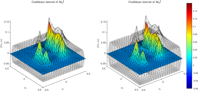
Figure 8: Confidence intervals for FAR regression and its debiased estimator.

Figure 10: Confidence intervals for $\textrm{AR}^{\kappa}$ regression and its debiased estimator.

References

- Abramowitz and Stegun (1972) Milton Abramowitz and Irene A. Stegun. Handbook of Mathematical Functions. Dover Publications, New York, 1972.
- Albani et al. (2016) Vinicius Albani, Peter Elbau, Maarten V. de Hoop, and Otmar Scherzer. Optimal convergence rates results for linear inverse problems in Hilbert spaces. Numerical Functional Analysis and Optimization, 37(5):521–540, 2016.
- Alexanderian et al. (2021) Alen Alexanderian, Noemi Petra, Georg Stadler, and Isaac Sunseri. Optimal design of large-scale Bayesian linear inverse problems under reducible model uncertainty: Good to know what you don’t know. SIAM/ASA Journal on Uncertainty Quantification, 9(1):163–184, 2021.
- Bakushinsky and Kokurin (2004) Anatoly Borisovich Bakushinsky and Mikhail Yuryevich Kokurin. Iterative Methods for Approximate Solution of Inverse Problems. Springer, New York, 2004.
- Bao and Li (2022) Gang Bao and Peijun Li. Maxwell’s Equations in Periodic Structures. Springer, Singapore, 2022.
- Bardsley and Hansen (2020) Johnathan M. Bardsley and Per Christian Hansen. MCMC algorithms for computational UQ of nonnegativity constrained linear inverse problems. SIAM Journal on Scientific Computing, 42(2):A1269–A1288, 2020.
- Bartlett et al. (2019) Peter L Bartlett, Nick Harvey, Christopher Liaw, and Abbas Mehrabian. Nearly-tight VC-dimension and pseudodimension bounds for piecewise linear neural networks. Journal of Machine Learning Research, 20(63):1–17, 2019.
- Batenburg et al. (2021) K. Joost Batenburg, Per Christian Hansen, and Jakob Jørgensen. Chapter 9: Discretization Models and the System Matrix, pages 155–181. SIAM, Philadelphia, 2021.
- Bauer et al. (2007) Frank Bauer, Sergei Pereverzev, and Lorenzo Rosasco. On regularization algorithms in learning theory. Journal of Complexity, 23(1):52–72, 2007.
- Benning and Burger (2018) Martin Benning and Martin Burger. Modern regularization methods for inverse problems. Acta Numerica, 27:1–111, 2018.
- Boţ et al. (2022) Radu Boţ, Guozhi Dong, Peter Elbau, and Otmar Scherzer. Convergence rates of first-and higher-order dynamics for solving linear ill-posed problems. Foundations of Computational Mathematics, 22(5):1567–1629, 2022.
- Bühlmann (2013) Peter Bühlmann. Statistical significance in high-dimensional linear models. Bernoulli, 19(4):1212–1242, 2013.
- Bühlmann and van de Geer (2011) Peter Bühlmann and Sara van de Geer. Statistics for High-Dimensional Data: Methods, Theory and Applications. Springer, Heidelberg, 2011.
- Chen et al. (2016) De-Han Chen, Bernd Hofmann, and Jun Zou. Elastic-net regularization versus -regularization for linear inverse problems with quasi-sparse solutions. Inverse Problems, 33(1):015004, 2016.
- Chernozhukov et al. (2013) Victor Chernozhukov, Denis Chetverikov, and Kengo Kato. Gaussian approximations and multiplier bootstrap for maxima of sums of high-dimensional random vectors. The Annals of Statistics, 41(6):2786–2819, 2013.
- Chernozhukov et al. (2018) Victor Chernozhukov, Denis Chetverikov, Mert Demirer, Esther Duflo, Christian Hansen, Whitney Newey, and James Robins. Double/debiased machine learning for treatment and structural parameters. The Econometrics Journal, 21(1):C1–C68, 2018.
- Chronopoulos et al. (2022) Ilias Chronopoulos, Katerina Chrysikou, and George Kapetanios. High dimensional generalised penalised least squares. arXiv preprint arXiv:2207.07055, 2022.
- Dassios and Fokas (2020) George Dassios and Athanassios S. Fokas. Electroencephalography and Magnetoencephalography: An Analytical-Numerical Approach. De Gruyter, Berlin, Boston, 2020.
- Daubechies et al. (2016) Ingrid Daubechies, Michel Defrise, and Christine De Mol. Sparsity-enforcing regularisation and ISTA revisited. Inverse Problems, 32(10):104001, 2016.
- Diethelm et al. (2004) Kai Diethelm, Neville J. Ford, and Alan D. Freed. Detailed error analysis for a fractional Adams method. Numerical Algorithms, 36(1):31–52, 2004.
- Ding and Han (2019) Liang Ding and Weimin Han. regularization for sparse recovery. Inverse Problems, 35(12):125009, 2019.
- Dou et al. (2022) Fangfang Dou, Xiaodong Liu, Shixu Meng, and Bo Zhang. Data completion algorithms and their applications in inverse acoustic scattering with limited-aperture backscattering data. Journal of Computational Physics, 469:111550, 2022.
- Droske and Bertozzi (2010) Marc Droske and Andrea Bertozzi. Higher-order feature-preserving geometric regularization. SIAM Journal on Imaging Sciences, 3(1):21–51, 2010.
- Engl et al. (1996) Heinz Werner Engl, Martin Hanke, and Andreas Neubauer. Regularization of Inverse Problems. Springer Netherlands, Dordrecht, 1996.
- Ernst et al. (2015) Oliver G. Ernst, Björn Sprungk, and Hans-Jörg Starkloff. Analysis of the ensemble and polynomial chaos Kalman filters in Bayesian inverse problems. SIAM/ASA Journal on Uncertainty Quantification, 3(1):823–851, 2015.
- Fan and Li (2001) Jianqing Fan and Runze Li. Variable selection via nonconcave penalized likelihood and its oracle properties. Journal of the American Statistical Association, 96(456):1348–1360, 2001.
- Fan et al. (2020) Jianqing Fan, Runze Li, Cun-Hui Zhang, and Hui Zou. Statistical Foundations of Data Science. Chapman & Hall/CRC, New York, 2020.
- Flath et al. (2011) H Pearl Flath, Lucas C Wilcox, Volkan Akçelik, Judith Hill, Bart van Bloemen Waanders, and Omar Ghattas. Fast algorithms for Bayesian uncertainty quantification in large-scale linear inverse problems based on low-rank partial Hessian approximations. SIAM Journal on Scientific Computing, 33(1):407–432, 2011.
- Frese et al. (2005) Udo Frese, Per Larsson, and Tom Duckett. A multilevel relaxation algorithm for simultaneous localization and mapping. IEEE Transactions on Robotics, 21(2):196–207, 2005.
- Galton (1886) Francis Galton. Regression towards mediocrity in hereditary stature. The Journal of the Anthropological Institute of Great Britain and Ireland, 15:246–263, 1886.
- Gong et al. (2020) Rongfang Gong, Bernd Hofmann, and Ye Zhang. A new class of accelerated regularization methods, with application to bioluminescence tomography. Inverse Problems, 36(5):055013, 2020.
- Gorenflo et al. (2014) Rudolf Gorenflo, Anatoly A. Kilbas, Francesco Mainardi, and Sergei Rogosin. Mittag-Leffler Functions, Related Topics and Applications. Springer-Verlag, Heidelberg, 2014.
- Grasmair et al. (2008) Markus Grasmair, Markus Haltmeier, and Otmar Scherzer. Sparse regularization with lq penalty term. Inverse Problems, 24(5):055020, 2008.
- Guo et al. (2014) Weihong Guo, Jing Qin, and Wotao Yin. A new detail-preserving regularization scheme. SIAM Journal on Imaging Sciences, 7(2):1309–1334, 2014.
- Guo and Cheng (2022) Xiao Guo and Guang Cheng. Moderate-dimensional inferences on quadratic functionals in ordinary least squares. Journal of the American Statistical Association, 117(540):1931–1950, 2022.
- Han et al. (2006) Weimin Han, Wenxiang Cong, and Ge Wang. Mathematical theory and numerical analysis of bioluminescence tomography. Inverse Problems, 22(5):1659, 2006.
- Hansen (2010) Per Christian Hansen. Discrete Inverse Problems: Insight and Algorithms. Society for Industrial and Applied Mathematics, Philadelphia, 2010.
- Hofmann and Mathé (2007) Bernd Hofmann and Peter Mathé. Analysis of profile functions for general linear regularization methods. SIAM Journal on Numerical Analysis, 45(3):1122–1141, 2007.
- Horn and Johnson (1985) Roger A. Horn and Charles R. Johnson. Matrix Analysis. Cambridge University Press, New York, 1985.
- Hosseini and Plataniotis (2020) Mahdi S. Hosseini and Konstantinos N. Plataniotis. Convolutional deblurring for natural imaging. IEEE Transactions on Image Processing, 29:250–264, 2020.
- Huang et al. (2023) Qin Huang, Rongfang Gong, Qinian Jin, and Ye Zhang. A Tikhonov regularization method for Cauchy problem based on a new relaxation model. Nonlinear Analysis: Real World Applications, 74:103935, 2023.
- Huang et al. (2024) Qin Huang, Rongfang Gong, and Ye Zhang. A new second-order dynamical method for solving linear inverse problems in hilbert spaces. Applied Mathematics and Computation, 473:128642, 2024.
- Isakov (1990) Victor Isakov. Inverse Source Problems. American Mathematical Society, New York, 1990.
- Ito and Jin (2014) Kazufumi Ito and Bangti Jin. Inverse Problems: Tikhonov Theory And Algorithms. World Scientific, Singapore, 2014.
- Ivanov et al. (2002) Valentin Konstantinovich Ivanov, Vladimir Vasilievich Vasin, and Vitalii Petrovich Tanana. Theory of linear ill-posed problems and its applications. Walter de Gruyter, Utrecht, 2002.
- Ivanov (1962) Vladimir Konstantinovich Ivanov. On linear ill-posed problems. Proceedings of the USSR Academy of Sciences, 145(2):270–272, 1962.
- Ivanov (1963) Vladimir Konstantinovich Ivanov. On ill-posed problems. Mathematics of the USSR. Sbornik, 61(2):211–223, 1963.
- Jiao et al. (2017) Yuling Jiao, Bangti Jin, and Xiliang Lu. Preasymptotic convergence of randomized Kaczmarz method. Inverse Problems, 33(12):125012, 2017.
- Johnson (2009) Claes Johnson. Numerical Solution of Partial Differential Equations by the Finite Element Method. Dover, New York, 2009.
- Kaipio and Somersalo (2005) Jari Kaipio and Erkki Somersalo. Statistical and Computational Inverse Problems. Springer, New York, 2005.
- Kaltenbacher et al. (2008) Barbara Kaltenbacher, Andreas Neubauer, and Otmar Scherzer. Iterative regularization methods for nonlinear ill-posed problems. Walter de Gruyter, Berlin, 2008.
- Kindermann (2021) Stefan Kindermann. Optimal-order convergence of nesterov acceleration for linear ill-posed problems. Inverse Problems, 37(6):065002, 2021.
- Knight and Fu (2000) Keith Knight and Wenjiang J. Fu. Asymptotics for lasso-type estimators. The Annals of Statistics, 28(5):1356–1378, 2000.
- Larson and Bengzon (2013) Mats G. Larson and Fredrik Bengzon. The Finite Element Method: Theory, Implementation, and Applications. Springer Science & Business Media, New York, 2013.
- Lavret’ev (1953) Mikhail Alekseevich Lavret’ev. On improving the accuracy of solution of a system of linear equations. Proceedings of the USSR Academy of Sciences, 92(5):885–886, 1953.
- Lavret’ev (1959) Mikhail Alekseevich Lavret’ev. On integral equations of the first kind. Proceedings of the USSR Academy of Sciences, 127(1):31–33, 1959.
- Li and Li (2022) Changcheng Li and Runze Li. Linear hypothesis testing in linear models with high-dimensional responses. Journal of the American Statistical Association, 117(540):1738–1750, 2022.
- Li et al. (2022) Jianliang Li, Peijun Li, and Xu Wang. Inverse source problems for the stochastic wave equations: Far-field patterns. SIAM Journal on Applied Mathematics, 82(4):1113–1134, 2022.
- Li (2023) Qing Li. A comprehensive survey of sparse regularization: Fundamental, state-of-the-art methodologies and applications on fault diagnosis. Expert Systems with Applications, 229:120517, 2023.
- Li et al. (2012) Runze Li, Wei Zhong, and Liping Zhu. Feature screening via distance correlation learning. Journal of the American Statistical Association, 107(499):1129–1139, 2012.
- Lopes (2014) Miles Lopes. A residual bootstrap for high-dimensional regression with near low-rank designs. In Advances in Neural Information Processing Systems, volume 27, page 3239–3247, 2014.
- Lorenz and Resmerita (2016) Dirk A Lorenz and Elena Resmerita. Flexible sparse regularization. Inverse Problems, 33(1):014002, 2016.
- Lu and Pereverzev (2013) Shuai Lu and Sergei V. Pereverzev. Regularization Theory for Ill-posed Problems: Selected Topics. Walter de Gruyter, Berlin, 2013.
- Mammen (1993) Enno Mammen. Bootstrap and wild bootstrap for high-dimensional linear models. The Annals of Statistics, 21(1):255–285, 1993.
- Martin and Tang (2020) Ryan Martin and Yiqi Tang. Empirical priors for prediction in sparse high-dimensional linear regression. Journal of Machine Learning Research, 21(144):1–30, 2020.
- Mathé (2004) Peter Mathé. Saturation of regularization methods for linear ill-posed problems in Hilbert spaces. SIAM Journal on Numerical Analysis, 42(3):968–973, 2004.
- Mathé and Pereverzev (2003) Peter Mathé and Sergei V. Pereverzev. Geometry of linear ill-posed problems in variable Hilbert scales. Inverse Problems, 19(3):789–803, 2003.
- Meng and Zhang (2024) Shixu Meng and Bo Zhang. A kernel machine learning for inverse source and scattering problems. SIAM Journal on Numerical Analysis, 62(3):1443–1464, 2024.
- Morozov (1966) Vladimir Alexandrovich Morozov. On the solution of functional equations by the method of regularization. Doklady Akademii Nauk SSSR, 167(3):510, 1966.
- Naseri et al. (2021) Arash Naseri, Timothy A. Sipkens, Steven Rogak, and Jason Olfert. An improved inversion method for determining two-dimensional mass distributions of non-refractory materials on refractory black carbon. Aerosol Science and Technology, 55(1):104–118, 2021.
- Nesterov (1983) Yurii Nesterov. A method for solving the convex programming problem with convergence rate O. Doklady Akademii Nauk SSSR, 269:543–547, 1983.
- Neubauer (2017) Andreas Neubauer. On Nesterov acceleration for Landweber iteration of linear ill-posed problems. Journal of Inverse and Ill-posed Problems, 25(3):381–390, 2017.
- Pearson (1896) Karl Pearson. VII. Mathematical contributions to the theory of evolution.—III. Regression, heredity, and panmixia. Philosophical Transactions of the Royal Society of London. Series A, containing papers of a mathematical or physical character, (187):253–318, 1896.
- Phillips (1962) David Lawrence Phillips. A technique for the numerical solution of certain integral equations of the first kind. Journal of the ACM, 9(1):84–97, 1962.
- Politis et al. (1999) Dimitris N. Politis, Joseph P. Romano, and Michael Wolf. Subsampling. Springer, New York, 1999.
- Radchenko and James (2010) Peter Radchenko and Gareth M. James. Variable selection using adaptive nonlinear interaction structures in high dimensions. Journal of the American Statistical Association, 105(492):1541–1553, 2010.
- Seber and Lee (2012) George A. F. Seber and Alan J. Lee. Linear regression analysis. John Wiley & Sons, Hoboken, second edition, 2012.
- Stefan et al. (2010) Wolfgang Stefan, Renaut A. Renaut, and Anne Gelb. Improved total variation-type regularization using higher order edge detectors. SIAM Journal on Imaging Sciences, 3(2):232–251, 2010.
- Szeg (1975) Gabor Szeg. Orthogonal Polynomials. American Mathematical Society, Providence, 1975.
- Tibshirani (1996) Robert Tibshirani. Regression shrinkage and selection via the lasso. Journal of the Royal Statistical Society: Series B, 58(1):267–288, 1996.
- Tichonov et al. (1998) Andrej Nikolaevich Tichonov, Aleksandr Sergeevič Leonov, and Anatolij Georgievich Jagola. Nonlinear Ill-Posed Problems. Chapman and Hall, London, 1998.
- Tikhonov (1963a) Andrei Nikolaevich Tikhonov. Regularization of incorrectly posed problems. Soviet Mathematics Doklady, 4:1624–1627, 1963a.
- Tikhonov (1963b) Andrei Nikolaevich Tikhonov. Solution of incorrectly formulated problems and the regularization method. Soviet Mathematics Doklady, 4:1035–1038, 1963b.
- Tong et al. (2018) Shanshan Tong, Bo Han, and Jinping Tang. Edge-guided TVp regularization for diffuse optical tomography based on radiative transport equation. Inverse Problems, 34(11):115009, 2018.
- Vainikko and Veretennikov (1986) Genrikh Mikhailovich Vainikko and Alexander Yuryevich Veretennikov. Iteration Procedures in Ill-Posed Problems (In Russian). Nauka, Moscow, 1986.
- van de Geer et al. (2011) Sara van de Geer, Peter Bühlmann, and Shuheng Zhou. The adaptive and the thresholded Lasso for potentially misspecified models (and a lower bound for the Lasso). Electronic Journal of Statistics, 5:688–749, 2011.
- Van der Vaart (2000) Aad W Van der Vaart. Asymptotic Statistics. Cambridge university press, Cambridge, 2000.
- Wang et al. (2013) Yanfei Wang, Ye Zhang, Dmitry Lukyanenko, and Anatoly Yagola. Recovering aerosol particle size distribution function on the set of bounded piecewise-convex functions. Inverse Problems in Science and Engineering, 21(2):339–354, 2013.
- Wang et al. (2024) Ying-Ao Wang, Qin Huang, Zhigang Yao, and Ye Zhang. On a class of linear regression methods. Journal of Complexity, 82:101826, 2024.
- Weinmann et al. (2014) Andreas Weinmann, Laurent Demaret, and Martin Storath. Total variation regularization for manifold-valued data. SIAM Journal on Imaging Sciences, 7(4):2226–2257, 2014.
- Whittle (1960) Peter Whittle. Bounds for the Moments of Linear and Quadratic Forms in Independent Variables. Theory of Probability and Its Applications, 5(3):302–305, 1960.
- Zhang and Zhang (2014) Cun-Hui Zhang and Stephanie S. Zhang. Confidence intervals for low dimensional parameters in high dimensional linear models. Journal of the Royal Statistical Society. Series B. Statistical Methodology, 76(1):217–242, 2014.
- Zhang and Wu (2017) Danna Zhang and Wei Biao Wu. Gaussian approximation for high dimensional time series. The Annals of Statistics, 45(5):1895–1919, 2017.
- Zhang and Cheng (2017) Xianyang Zhang and Guang Cheng. Simultaneous inference for high-dimensional linear models. Journal of the American Statistical Association, 112(518):757–768, 2017.
- Zhang et al. (2017) Xiongjun Zhang, Minru Bai, and Michael K. Ng. Nonconvex-TV based image restoration with impulse noise removal. SIAM Journal on Imaging Sciences, 10(3):1627–1667, 2017.
- Zhang (2023) Ye Zhang. On the acceleration of optimal regularization algorithms for linear ill-posed inverse problems. Calcolo, 60(1):6, 2023.
- Zhang and Chen (2022) Ye Zhang and Chuchu Chen. Stochastic asymptotical regularization for linear inverse problems. Inverse Problems, 39(1):015007, 2022.
- Zhang and Gong (2020) Ye Zhang and Rongfang Gong. Second order asymptotical regularization methods for inverse problems in partial differential equations. Journal of Computational and Applied Mathematics, 375:112798, 2020.
- Zhang and Hofmann (2019) Ye Zhang and Bernd Hofmann. On fractional asymptotical regularization of linear ill-posed problems in Hilbert spaces. Fractional Calculus and Applied Analysis, 22(3):699–721, 2019.
- Zhang and Hofmann (2020) Ye Zhang and Bernd Hofmann. On the second-order asymptotical regularization of linear ill-posed inverse problems. Applicable Analysis, 99(6):1000–1025, 2020.
- Zhang and Hofmann (2021) Ye Zhang and Bernd Hofmann. Two new non-negativity preserving iterative regularization methods for ill-posed inverse problems. Inverse Problems and Imaging, 15(2):229–256, 2021.
- Zhang et al. (2016) Ye Zhang, Mårten Gulliksson, VM Hernandez Bennetts, and Erik Schaffernicht. Reconstructing gas distribution maps via an adaptive sparse regularization algorithm. Inverse Problems in Science and Engineering, 24(7):1186–1204, 2016.
- Zhang et al. (2018a) Ye Zhang, Patrik Forssén, Torgny Fornstedt, Mårten Gulliksson, and Xiaoxia Dai. An adaptive regularization algorithm for recovering the rate constant distribution from biosensor data. Inverse Problems in Science and Engineering, 26(10):1464–1489, 2018a.
- Zhang et al. (2018b) Ye Zhang, Rongfang Gong, Xiaoliang Cheng, and Mårten Gulliksson. A dynamical regularization algorithm for solving inverse source problems of elliptic partial differential equations. Inverse Problems, 34(6):065001, 2018b.
- Zhang et al. (2019) Ye Zhang, Zhigang Yao, Patrik Forssén, and Torgny Fornstedt. Estimating the rate constant from biosensor data via an adaptive variational bayesian approach. Annals of Applied Statistics, 13:2011–2042, 2019.
- Zhang and Politis (2023) Yunyi Zhang and Dimitris N. Politis. Debiased and thresholded ridge regression for linear models with heteroskedastic and correlated errors. Journal of the Royal Statistical Society. Series B. Statistical Methodology, 85(2):327–355, 2023.
- Zhang and Politis (2020) Yunyi Zhang and Dimitris Nicolas Politis. Ridge regression revisited: Debiasing, thresholding and bootstrap. The Annals of Statistics, 50(3):1401–1422, 2020.
- Zhao and Yu (2006) Peng Zhao and Bin Yu. On model selection consistency of Lasso. Journal of Machine Learning Research, 7:2541–2563, 2006.