A Jacobian-free Newton-Krylov method for cell-centred finite volume solid mechanics

Abstract

This study investigates the efficacy of Jacobian-free Newton-Krylov methods in finite-volume solid mechanics. Traditional Newton-based approaches require explicit Jacobian matrix formation and storage, which can be computationally expensive and memory-intensive. In contrast, Jacobian-free Newton-Krylov methods approximate the Jacobian’s action using finite differences, combined with Krylov subspace solvers such as the generalised minimal residual method (GMRES), enabling seamless integration into existing segregated finite-volume frameworks without major code refactoring. This work proposes and benchmarks the performance of a compact-stencil Jacobian-free Newton-Krylov method against a conventional segregated approach on a suite of test cases, encompassing varying geometric dimensions, nonlinearities, dynamic responses, and material behaviours. Key metrics, including computational cost, memory efficiency, and robustness, are evaluated, along with the influence of preconditioning strategies and stabilisation scaling. Results show that the proposed Jacobian-free Newton-Krylov method outperforms the segregated approach in all linear and nonlinear elastic cases, achieving order-of-magnitude speedups in many instances; however, divergence is observed in elastoplastic cases, highlighting areas for further development. It is found that preconditioning choice impacts performance: a LU direct solver is fastest in small to moderately-sized cases, while a multigrid method is more effective for larger problems. The findings demonstrate that Jacobian-free Newton-Krylov methods are promising for advancing finite-volume solid mechanics simulations, particularly for existing segregated frameworks where minimal modifications enable their adoption. The described implementations are available in the solids4foam toolbox for OpenFOAM, inviting the community to explore, extend, and compare these procedures.

1 Introduction

Finite volume formulations for solid mechanics are heavily influenced by their fluid mechanics counterparts, favouring fully explicit [1, 2, 3, 4] or segregated implicit [5, 6, 7, 8, 9, 10, 11, 12] methods. Segregated approaches, where the governing equations are temporarily decomposed into scalar component equations, offer memory efficiency and simplicity of implementation, but the outer coupling Picard iterations often suffer from slow convergence. Explicit formulations are straightforward to implement and offer superior robustness but are only efficient for high-speed dynamics, where the physics requires small time increments. In contrast, the finite element community commonly employs Newton-Raphson-type solution algorithms, which necessitate repeated assembly of the Jacobian matrix and solution of the resulting block-coupled non-diagonally dominant linear system. A disadvantage of traditional Newton-based approaches is that they typically require explicit formation and storage of the Jacobian matrix, which can be computationally expensive and memory-intensive. A further disadvantage from a finite volume perspective is that extending existing code frameworks from segregated algorithms to coupled Newton-Raphson-type approaches is challenging in terms of the required assembly, storage, and solution of the resulting block-coupled system. In addition, the derivation of the true Jacobian matrix is non-trivial. Consequently, similar block-coupled solution finite volume methods are rare in the literature [13, 14, 15]. The motivation of the current work is to seek the robustness and efficiency of block-coupled Newton-Raphons approaches in a way that can be easily incorporated into existing segregated solution frameworks. To this end, the current article proposes and examines the efficacy of Jacobian-free Newton-Krylov methods, where the quadratic convergence of Newton methods can potentially be achieved without deriving, assembling and storing the exact Jacobian.

Jacobian-free Newton-Krylov methods circumvent the need for the Jacobian matrix by combining the Newton-Raphson method with Krylov subspace iterative linear solvers, such as the generalised minimal residual method (GMRES), and noticing that such Krylov solvers do not explicitly require the Jacobian matrix. Instead, only the action of the Jacobian matrix on a solution-type vector is required. The key step in Jacobian-free Newton-Krylov methods is the approximation of products between the Jacobian matrix and a vector using the finite difference method; that is

$$\bm{J}\bm{v}\approx\frac{\bm{R}(\bm{u}+\epsilon\bm{v})-\bm{R}(\bm{u})}{\epsilon}$$ (1)

where $\bm{J}$ is the Jacobian matrix, $\bm{R}$ is the residual function of the governing equation, $\mathbf{u}$ is the current solution vector (e.g. nodal displacements), $\mathbf{v}$ is a vector (e.g., from a Krylov subspace), and $\epsilon$ is a small scalar perturbation. With an appropriate choice of $\epsilon$ (balancing truncation and round-off errors), the characteristic quadratic convergence of Newton methods can be achieved without the Jacobian, hence the modifier Jacobian-free. This approach promises significant memory savings over Jacobian-based methods, especially for large-scale problems, but also potentially for execution time, with appropriate choice of solution components.

A crucial aspect of ensuring the efficiency and robustness of the Jacobian-free Newton-Krylov method is the choice of a suitable preconditioner for the Krylov iterations. This preconditioner is often derived from the exact Jacobian matrix in traditional Newton methods. However, the Jacobian-free approach does not allow direct access to the full Jacobian matrix, necessitating an alternative strategy to approximate its action. To this end, and to extend existing segregated frameworks, this work proposes using a compact-stencil approximate Jacobian as the preconditioner. This approximate Jacobian corresponds to the matrix typically employed in segregated solid mechanics approaches; similar approaches are successful in fluid mechanics applications [16, 17, 18, 19, 20, 21, 22, 23, 24, 25]; however, it is unclear if such an approach is suitable for solid mechanics - a question this work aims to answer. By leveraging this compact-stencil approximate Jacobian, it is aimed to effectively precondition the Krylov iterations, enhancing convergence while maintaining the memory and computational savings that define the Jacobian-free and segregated methods. Similarly, if such an approach is efficient, it would naturally fit into existing segregated frameworks, as existing matrix storage and assembly can be reused.

As noted by Knoll and Keyes [20], Jacobian-free Newton–Krylov methods first appeared in the 1980s and early 1990s for the solution of ordinary and partial differential equations [26, 27, 28, 29]. McHugh and Knoll [16] and co-workers demonstrated the potential of Jacobian-free Newton-Krylov approaches for the solution of steady, incompressible, Navier-Stokes problems using a staggered finite volume formulation. They found the GMRES linear solver to be faster than a conjugate solver, however, the true Jacobian matrix was still evalauted by finite differencing in the construction of the preconditioning matrix. Qin et al. [17] later extended Jacobian-free Newton–Krylov methods to unsteady compressible Reynolds-averaged Navier–Stokes equations. Once again it was found that GMRES was more robust than a conjugate gradient linear solver. For preconditioning, a fully matrix-free approach was proposed, based on the approximate factorization procedure of Badcock and Gaitonde [30]. Geuzaine [18] examined the use of lower and higher-order discretisations for the preconditioning matrix for steady, compressible high Reynolds number flows. They found that the lower-order compact stencil preconditioner gave the best performance when combined with the GMRES linear solver and ILU($k$) preconditioner. As is common with other Newton approaches, a pseudo transient algorithm and mesh sequencing strategy were used to improve the convergence. With the aim of exploiting mature segregated solution approaches, Pernice and Tocci [19] recast the SIMPLE segregated algorithm as a method which operators on residuals, allowing it to act as the preconditioner for a Jacobian-free Newton-Krylov approach. It was found that the SIMPLE-preconditioned Jacobian-free Newton-Krylov substantially accelerated convergence for the incompressible Navier–Stokes problems examined. GMRES was the adopted linear solver, where the importance of choosing an appropriate restart parameter was noted. They also found a multigrid approach to be more efficient than ILU($k$) for preconditioning, where the implementation was based on the PETSc [31] package.

Over the subsequent two decades, Jacobian-free Newton-Krylov methods have seen increasing application in the field of finite volume computational fluid dynamics, albeit they are still far from widespread. The use of low-order approximate Jacobians for preconditioning has been established as an efficient and robust approach, e.g. [21, 22, 24, 25]. A particularly attractive application of the low-order preconditioning approach is for higher-order discretisations; that is, spatial discretisation of order greater than two. Nejat and Ollivier-Gooch [21] demonstrated such a higher order approach for steady, inviscid compressible flows, with up to fourth order accuracy. GMRES was the adopted linear solver with the ILU($k$) preconditioner and fill-in values ($k$) ranging from 2 to 4. Nejat et al. [24] later applied the second-order variant of the approach to non-Newtonian flows and found Newton-GMRES with ILU(1) to be the most efficient combination. Like Vaassen et al. [22] and many other authors, Nejat and co-workers [21, 24] proposed a special start-up phase to encourage the solution to efficiently reach the Newton method’s domain of quadratic convergence. The use of a pseudo-transient approach combined with an adaptive time step (e.g., based on the convergence of the Newton iterations) is common. A further promotion for the benefit of Jacobian-free Newton-Krylov methods in fluid dynamics was provided by Lucas et al. [23], who demonstrated order of magnitude speedups over nonlinear multigrid methods. A particular benefit was the insensitivity of the Jacobian-free Newton-Krylov methods to changes in mesh aspect ratio, density, time step and Reynolds number. A final relevant point is the effect of numerical stabilisation (damping) on the convergence: Nishikawa et al. [32] demonstrated that a Jacobian-free Newton-Krylov approach was less sensitive to the magnitude of the damping and remained stable for lower values of damping compared with a segregated approach.

Although they are increasingly seen in finite volume computational fluid dynamics, Jacobian-free Newton-Krylov methods have yet to be used for finite volume solid mechanics. This article aims to address this point by assessing the efficacy of Jacobian-free Newton-Krylov cell-centred finite volume formulations applied to static, dynamic, linear and nonlinear solid mechanics problems. Particular focus is given to the use of a compact-stencil approximate Jacobian preconditioner, inspired from existing segregated solid mechanics procedures, and ease of implementation into an existing segregated finite volume framework – OpenFOAM [33]. The remainder of the paper is structured as follows: Section 2 summarises a typical solid mechanics mathematical model and its cell-centred finite volume discretisation. Section 3 presents the solution algorithms, starting with the classic segregated solution algorithm, followed by the proposed Jacobian-free Newton-Krylov solution algorithm. The performance of the proposed Jacobian-free Newton-Krylov approach is compared with the segregated approach on several varying benchmark cases in Section 4, where the effect of several factors are examined. Finally, the article ends with a summary of the main conclusions of the work.

2 Mathematical Model and Numerical Methods

2.1 Governing Equations

In this work, interest is restricted to Lagrangian formulations of the conservation of linear momentum. Assuming small strains, the linear geometry formulation is expressed in strong integral form as:

$$\int_{\Omega}\rho\frac{\partial^{2}\bm{u}}{\partial t^{2}}\,d\Omega=\oint_{\Gamma}\bm{n}\cdot\bm{\sigma}_{s}\,d\Gamma+\int_{\Omega}\bm{f}_{b}\,d\Omega$$ (2)

where $\Omega$ is the volume of an arbitrary body bounded by a surface $\Gamma$ with outwards pointing normal $\bm{n}$. The density is $\rho$, $\bm{u}$ is the displacement vector, $\bm{\sigma}_{s}$ is the engineering (small strain) stress tensor, and $\bm{f}_{b}$ is a body force per unit volume, e.g., $\rho\bm{g}$, where $\bm{g}$ is gravity.

More generally, linear momentum conservation can be expressed in a nonlinear geometry form, which is suitable for finite strains. Two equivalent nonlinear geometry forms are common: the total Lagrangian form:

$$\int_{\Omega_{o}}\rho_{o}\frac{\partial^{2}\bm{u}}{\partial t^{2}}d\Omega_{o}=\oint_{\Gamma_{o}}\left(J\bm{F}^{-\text{T}}\cdot\bm{n}_{o}\right)\cdot\bm{\sigma}\ d\Gamma_{o}+\int_{\Omega_{o}}\bm{f}_{b}\,d\Omega_{o}$$ (3)

and the updated Lagrangian form:

$$\int_{\Omega_{u}}\frac{\partial}{\partial t}\left(\rho_{u}\frac{\partial\bm{u}}{\partial t}\right)d\Omega_{u}=\oint_{\Gamma_{u}}(j\bm{f}^{-\text{T}}\cdot{\bm{n}_{u})\cdot\bm{\sigma}}\ d\Gamma_{u}+\int_{\Omega_{u}}\bm{f}_{b}\,d\Omega_{u}$$ (4)

where subscript $o$ indicates quantities in the initial reference configuration, and subscript $u$ indicates quantities in the updated configuration. The true (Cauchy) stress tensor is indicated by $\bm{\sigma}$. The deformation gradient is defined as $\bm{F}=\textbf{I}+(\bm{\nabla}\bm{u})^{\text{T}}$ and its determinant as $J=\text{det}(\bm{F})$. Similarly, the relative deformation gradient is given in terms of the displacement increment as $\bm{f}=\textbf{I}+\left[\bm{\nabla}(\Delta\bm{u})\right]^{\text{T}}$ and its determinant as $j=\text{det}(\bm{f})$. The displacement increment is the change in displacement between the current time step and the previous time step when the time interval is discretised into a finite number of steps.

The governing equations are complemented by boundary conditions, with three types considered here: prescribed displacement, prescribed traction, and symmetry. The definition of the engineering stress ($\bm{\sigma}_{s}$) and true stress ($\bm{\sigma}$) in Equations 2, 3 and 4 is given by a chosen mechanical law. Five mechanical laws are considered in this work, as briefly outlined in Appendix A: linear elasticity (Hooke’s law), three forms of hyperelasticity (St. Venant-Kirchhoff, neo-Hookean, and Guccione), and neo-Hookean $J_{2}$ hyperelastoplasticity.

2.2 Newton-Type Solution Methods

To facilitate the comparison between the classic segregated solution algorithm and the proposed Jacobian-free Newton-Krylov algorithm, the governing linear momentum conservation (Equations 2, 3 and 4) is expressed in the general form:

$$\bm{R}(\bm{u})=\bm{0}$$ (5)

where $\bm{R}$ represents the residual (imbalance) of the equation, which is a function of the primary unknown field. For example, in the linear geometry case, the residual is given as

$$\bm{R}(\bm{u})\;=\;\oint_{\Gamma}\bm{n}\cdot\bm{\sigma}_{s}(\bm{u})\,d\Gamma+\int_{\Omega}\rho\bm{g}\,d\Omega-\int_{\Omega}\rho\frac{\partial^{2}\bm{u}}{\partial t^{2}}\,d\Omega\;=\;\bm{0}$$ (6)

where the dependence of the stress tensor on the solution vector is made explicitly clear: $\bm{\sigma}_{s}(\bm{u})$.

In Newton-type methods, a Taylor expansion about a current point $\bm{u}_{k}$ can be used to solve Equation 5 [20]:

$$\bm{R}(\bm{u}_{k+1})=\bm{R}(\bm{u}_{k})\;+\;\bm{R}^{\prime}(\bm{u}_{k})(\bm{u}_{k+1}-\bm{u}_{k})\;+\;\text{H.O.T.}=\bm{0}$$ (7)

Neglecting the higher-order terms (H.O.T.) yields the strict Newton method in terms of an iteration over a sequence of linear systems:

$$\bm{J}(\bm{u}_{k})\delta\bm{u} = -\bm{R}(\bm{u}_{k}),$$

$$\bm{u}_{k+1} = \bm{u}_{k}+s\,\delta\bm{u},$$

$$\quad k = 0,1,...$$ (8)

where $\bm{J}\equiv\bm{R}^{\prime}\equiv\partial\bm{R}/\partial\bm{u}$ is the Jacobian matrix. Starting the Newton procedure requires the specification of $\bm{u}_{0}$. The scalar $s>0$ can be chosen to improve convergence, for example, using a line search or under-relaxation/damping procedure, and is equal to unity in the classic Newton-Raphson approach. Iterations are performed over this system until the residual $\bm{R}(\bm{u}_{k})$ and solution correction $\delta\bm{u}$ are sufficiently small, with appropriate normalisation.

For problems with $N$ scalar equations and $N$ scalar unknowns, the residual $\bm{R}$ and solution $\bm{u}$ vectors have dimensions of $N\times 1$. The components of the $N\times N$ Jacobian are

$${J}_{ij}=\frac{\partial{R}_{i}(\bm{u})}{\partial u_{j}}$$ (9)

The current work focuses on vector problems, where the governing momentum equation is formulated in terms of the unknown displacement solution vector. In this case, Equation 9 refers to the individual scalar components of the residual, solution, and Jacobian. That is, for 3-D analyses, the residual takes the form

$$\bm{R}(\bm{u})=\left\{R_{1}^{x},R_{1}^{y},R_{1}^{z},R_{2}^{x},R_{2}^{y},R_{2}^{z},...,R_{n}^{z}\right\}$$ (10)

and the solution takes the form

$$\bm{u}=\left\{u_{1}^{x},u_{1}^{y},u_{1}^{z},u_{2}^{x},u_{2}^{y},u_{2}^{z},...,u_{n}^{z}\right\}$$ (11)

In practice, it is often more practical and efficient to form and store the residual, solution and Jacobian in a blocked manner, where the residual and solution can be considered as vectors of vectors. Similarly, the Jacobian can be formed in terms of sub-matrix block coefficients.

In the strict Newton procedure, the residuals converge at a quadratic rate when the current solution is close to the true solution; that is, the iteration error decreases proportionally to the square of the error at the previous iteration. Once the method gets sufficiently close to the true solution, the number of correct digits in the approximation roughly doubles with each iteration. However, quadratic convergence is only possible when using the exact Jacobian. In contrast, a quasi-Newton method uses an approximation to the Jacobian, sacrificing strict quadratic convergence in an attempt to produce an overall more computationally efficient procedure. From this perspective, the segregated solution algorithm commonly employed in finite volume solid mechanics can be viewed as a quasi-Newton method, where an approximate Jacobian replaces the exact Jacobian:

$$\bm{\tilde{J}}(\bm{u}_{k})\;\delta\bm{u}=-\bm{R}(\bm{u}_{k})$$ (12)

In this case, the approximate Jacobian $\bm{\tilde{J}}$ comes from the compact stencil discretisation of a simple diffusion (Laplacian) term inertia terms. A benefit of this approach is that the inter-component coupling is removed from the Jacobian, allowing the solution of three smaller scalar systems rather than one larger vector system in 3-D (or two smaller systems in 2-D).

A fully explicit procedure can also be viewed from this perspective by selecting a diagonal approximate Jacobian $\bm{\tilde{D}}$ (only the inertia term), making the solution of the linear system trivial:

$$\bm{\tilde{D}}(\bm{u}_{k})\;\delta\bm{u}=-\bm{R}(\bm{u}_{k})$$ (13)

2.3 Cell-Centred Finite Volume Discretisation

In this work, a nominally second-order cell-centred finite volume discretisation is employed. The solution domain is discretised in both space and time. The total simulation period is divided into a finite number of time increments, denoted as $\Delta t$, and the discretised governing momentum equation is solved iteratively in a time-marching fashion. The spatial domain is partitioned into a finite set $\mathcal{P}$ of contiguous convex polyhedral cells, where each cell is denoted by $P\in\mathcal{P}$. The number of cells in the mesh is indicated by $|\mathcal{P}|$. A representative cell $P$ is shown in Figure 1. The set of all faces of cell $P$ is denoted by $\mathcal{F}_{P}$. This set is further subdivided into two disjoint subsets:

• Internal Faces ($\mathcal{F}^{\text{int}}_{P}$): Faces that are shared with neighbouring cells.

• Boundary Faces ($\mathcal{F}^{\text{bnd}}_{P}$): Faces that lie on the boundary of the spatial domain. The boundary faces of cell $P$ are further classed into three disjoint sets, $\mathcal{F}^{\text{bnd}}_{P}\coloneqq\mathcal{F}^{\text{disp}}_{P}\cup\mathcal{F}^{\text{trac}}_{P}\cup\mathcal{F}^{\text{symm}}_{P}$, representing boundary faces where displacement ($\mathcal{F}^{\text{disp}}_{P}$), traction ($\mathcal{F}^{\text{trac}}_{P}$) and symmetry ($\mathcal{F}^{\text{symm}}_{P}$) conditions are prescribed.

Each internal face $f_{i}\in\mathcal{F}^{\text{int}}_{P}$ corresponds to a neighbouring cell $N_{f_{i}}\in\mathcal{N}_{P}$, where $\mathcal{N}_{P}$ is the set of all neighbouring cells of $P$. The outward unit normal vector associated with an internal face $f_{i}$ is denoted by $\mathbf{n}_{f_{i}}$, while the outward unit normal vector associated with a boundary face $b_{i}$ is denoted by $\mathbf{n}_{b_{i}}$. The vector $\mathbf{d}_{f_{i}}$ connects the centroid of cell $P$ with the centroid of the neighbouring cell $N_{f_{i}}$, whereas the vector $\mathbf{d}_{b_{i}}$ connects the centroid of cell $P$ with the centroid of boundary face ${b_{i}}$. For convenience, we will also define the set of all faces of cell $P$ excluding those on a traction boundary as $\mathcal{F}_{P}^{\text{non-trac}}\coloneqq\mathcal{F}_{P}^{\text{int}}\cup\mathcal{F}_{P}^{\text{disp}}\cup\mathcal{F}_{P}^{\text{symm}}$.

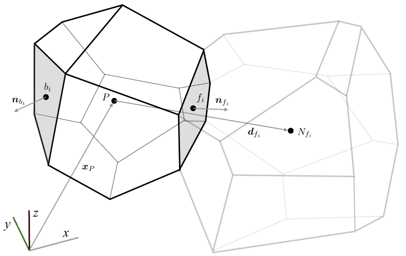
Figure 1: Representative convex polyhedral cell $P$ and neighbouring cell $N_{f_{i}}$, which share a face $f_{i}$.

The conservation equation (Equations 2, 3, or 4) is applied to each cell $P$ and discretised in terms of the displacement at the centroid of the cell $\bm{u}_{P}$ and the displacements $\bm{u}_{N_{f_{i}}}$ at the centroids of the neighbouring cells. Proceeding with the discretisation, the volume and surface integrals in the governing equation are approximated by algebraic equations as described below.

2.3.1 Volume Integrals

To discretise the volume integrals, the integrand $\bm{\phi}$ is assumed to locally vary according to a truncated Taylor series expansion about the centroid of cell $P$:

$$\bm{\phi}(\bm{x})\approx\bm{\phi}_{P}+(\bm{x}-\bm{x}_{P})\cdot\nabla\bm{\phi}_{P}$$ (14)

where subscript $P$ indicates a value at the centroid of the cell $P$. Consequently, volume integrals over a cell $P$ can be approximated to second-order accuracy as

$$\int_{\Omega_{P}}\bm{\phi}\,d\Omega_{P} \approx \int_{\Omega_{P}}\left[\bm{\phi}_{P}+(\bm{x}-\bm{x}_{P})\cdot\nabla\bm{\phi}_{P}\right]d\Omega_{P}$$ (15)

$$\approx \bm{\phi}_{P}\Omega_{P}$$

where $\Omega_{P}$ is the volume of cell $P$ and $\int_{\Omega_{P}}(\bm{x}-\bm{x}_{P})d\Omega_{P}\equiv 0$ by definition of the cell centroid. This approximation corresponds to the midpoint rule and one point quadrature.

Using Equation 15, the inertia term (e.g. left-hand side term of Equation 2) becomes

$$\int_{\Omega_{P}}\rho\frac{\partial\bm{u}}{\partial t}d\Omega_{P}\; \approx \;\rho_{P}\left(\frac{\partial^{2}\bm{u}}{\partial t^{2}}\right)_{P}\Omega_{P}$$ (16)

Similarly, the body force term (e.g. the second term on the right-hand side of Equation 2) becomes:

$$\int_{\Omega_{P}}\,\rho\,\bm{g}\,d\Omega_{P}\; \approx \;\rho_{P}\,\bm{g}\,\Omega_{P}$$ (17)

The discretisation of the acceleration in Equation 16 can be achieved using one of many finite difference schemes, e.g. first-order Euler, second-order backwards, or second-order Newmark-beta. In the current work, the second-order backwards (BDF2) scheme is used:

$$\left(\frac{\partial^{2}\bm{u}_{P}}{\partial t^{2}}\right)_{P} \approx \frac{3\bm{v}_{P}^{[t+1]}-4\bm{v}_{P}^{[t]}+\bm{v}_{P}^{[t-1]}}{2\Delta t}$$ (18)

$$\approx \frac{3\left(\dfrac{3\bm{u}_{P}^{[t+1]}-4\bm{u}_{P}^{[t]}+\bm{u}_{P}^{[t-1]}}{2\Delta t}\right)-4\bm{v}_{P}^{[t]}+\bm{v}_{P}^{[t-1]}}{2\Delta t}$$

where $\Delta t$ is the time increment – assumed constant here. Superscript $[t]$ indicates the time level, with $\bm{u}_{P}^{[t+1]}$ corresponding to the unknown displacement at the current time step. The velocity vector $\bm{v}=\partial\bm{u}/\partial t$ at the current time step is also updated using the BDF2 scheme as

$$\bm{v}_{P}^{[t+1]} \approx \dfrac{3\bm{u}_{P}^{[t+1]}-4\bm{u}_{P}^{[t]}+\bm{u}_{P}^{[t-1]}}{2\Delta t}$$ (19)

Consequently, the displacement and velocity at the two previous time steps must be stored, or alternatively, the displacement at the previous four time steps.

2.3.2 Surface Integrals

The surface integral term can be discretised using one-point quadrature at each face $f_{i}$ as

$$\oint_{\Gamma_{P}}\bm{n}\cdot\bm{\sigma}\;d\Gamma_{P} = \sum_{f_{i}\in\mathcal{F}_{P}}\int_{\Gamma_{f_{i}}}\bm{n}\cdot\bm{\sigma}\,d\Gamma_{f_{i}}$$ (20)

$$\approx \sum_{f_{i}\in\mathcal{F}_{P}^{\text{int}}}\bm{\Gamma}_{f_{i}}\cdot\bm{\sigma}_{f_{i}}+\sum_{d_{i}\in\mathcal{F}_{P}^{\text{disp}}}\bm{\Gamma}_{d_{i}}\cdot\bm{\sigma}_{P}+\sum_{s_{i}\in\mathcal{F}_{P}^{\text{symm}}}\bm{\Gamma}_{s_{i}}\cdot\bm{\sigma}_{s_{i}}+\sum_{t_{i}\in\mathcal{F}_{P}^{\text{trac}}}|\bm{\Gamma}_{t_{i}}|\bar{\bm{T}}_{t_{i}}$$

where $\Gamma_{P}$ indicates the surface of cell $P$, $\bm{\Gamma}_{f_{i}}$ indicates the area vector of face $f_{i}$, and vector $\bar{\bm{T}}_{t_{i}}$ represents the prescribed traction on the traction boundary face $t_{i}$.

It is noted that the displacement is assumed to vary linearly within each cell; hence, the displacement gradient and stress are constant within each cell. In the current work, a unique definition of stress $\bm{\sigma}_{f_{i}}$ at each cell face $f_{i}$ is given as a weighted-averaged of values in the two cells ($\bm{\sigma}_{P}$, $\bm{\sigma}_{N_{f_{i}}}$) straddling the face [34]:

$$\bm{\sigma}_{f_{i}} = w_{f_{i}}\bm{\sigma}_{P}+(1-w_{f_{i}})\bm{\sigma}_{N_{f_{i}}}$$ (21)

where the interpolation weight is defined as $w_{f_{i}}=(\bm{n}_{f_{i}}\cdot[\bm{x}_{N_{f_{i}}}-\bm{x}_{f_{i}}])/(\bm{n}_{f_{i}}\cdot[\bm{x}_{N_{f_{i}}}-\bm{x}_{P}])$; however, achieving second-order accuracy of the displacement field is independent of the value of the weights, and, for example, $w_{f_{i}}=\nicefrac{{1}}{{2}}$ would also be sufficient.

The stress $\bm{\sigma}_{s_{i}}$ at a symmetry boundary face is calculated as

$$\bm{\sigma}_{s_{i}} = \frac{1}{2}\left(\bm{\sigma}_{P}+\bm{R}_{s_{i}}\cdot\bm{\sigma}_{P}\right)$$ (22)

$$= \left(\textbf{I}-\bm{n}_{s_{i}}\otimes\bm{n}_{s_{i}}\right)\cdot\bm{\sigma}_{P}$$

where $\bm{R}_{s_{i}}\cdot\bm{\sigma}_{P}$ represents the mirror reflection of $\bm{\sigma}_{P}$ across the symmetry boundary face $s_{i}$. The reflection tensor is $\bm{R}_{s_{i}}=\textbf{I}-2\bm{n}_{s_{i}}\otimes\bm{n}_{s_{i}}$ [35], with $\bm{n}_{s_{i}}$ indicating the unit normal of the symmetry boundary face $s_{i}$. From Equation 22, it is clear that shear stresses are zero on a symmetry plane boundary face. Note from Equation 20 that the stress on displacement boundary faces is assumed to be equal to the stress $\bm{\sigma}_{P}$ at the centroid of cell $P$.

The cell-centred stress $\bm{\sigma}_{P}$ is calculated as a function of the displacement gradient according to the chosen mechanical law, for example, as shown in Appendix A. The presented discretisation is second-order accurate in space for displacement if the cell-centred displacement gradients (and the stress) are at least first-order accurate in space, even if the cell faces are not flat. To achieve this, the cell-centred displacement gradients are determined using a weighted first-neighbours least squares method [34],

$$\left(\bm{\nabla}\bm{u}\right)_{P} = \sum_{f_{i}\in\mathcal{F}^{\text{int}}_{P}}w_{f_{i}}|\bm{\Gamma}_{f_{i}}|\frac{\bm{G}^{-1}_{P}\cdot\bm{d}_{f_{i}}}{\bm{d}_{f_{i}}\cdot\bm{d}_{f_{i}}}\otimes\left(\bm{u}_{N_{f_{i}}}-\bm{u}_{P}\right)$$ (23)

$$+\sum_{d_{i}\in\mathcal{F}^{\text{disp}}_{P}}w_{f_{i}}|\bm{\Gamma}_{d_{i}}|\frac{\bm{G}^{-1}_{P}\cdot\bm{d}_{d_{i}}}{\bm{d}_{d_{i}}\cdot\bm{d}_{d_{i}}}\otimes\left(\bm{u}_{d_{i}}-\bm{u}_{P}\right)$$

$$+\sum_{s_{i}\in\mathcal{F}^{\text{symm}}_{P}}w_{f_{i}}|\bm{\Gamma}_{s_{i}}|\frac{\bm{G}^{-1}_{P}\cdot\bm{d}_{s_{i}}}{\bm{d}_{s_{i}}\cdot\bm{d}_{s_{i}}}\otimes\left(\bm{R}_{s_{i}}\cdot\bm{u}_{P}-\bm{u}_{P}\right)$$

which is exact for linear functions. The vector $\bm{u}_{b_{i}}$ indicates the displacement at the centroid of boundary face ${b_{i}}$, while vector $\bm{d}_{d_{i}}$ connects the centroid of cell $P$ to the centroid of displacement boundary face $d_{i}$. The quantity $\bm{R}_{s_{i}}\cdot\bm{u}_{P}$ represents the mirror reflection of $\bm{u}_{P}$ across the symmetry boundary face $s_{i}$. The vector $\bm{d}_{s_{i}}$ connects the centroid $\bm{x}_{P}$ of cell $P$ with its mirror reflection $\bm{R}_{s_{i}}\cdot\bm{x}_{P}$ through boundary face $s_{i}$. Traction boundary faces are excluded in Equation 23, as the displacement is unknown there; this is in contrast to the default approach in OpenFOAM [36]. The $\bm{G}_{P}$ tensor for cell $P$ is calculated as

$$\bm{G}_{P} = \sum_{{f_{i}}\in\mathcal{F}^{\text{int}}_{P}}(1-w_{f_{i}})|\bm{\Gamma}_{f_{i}}|\frac{\bm{d}_{f_{i}}\otimes\bm{d}_{f_{i}}}{\bm{d}_{f_{i}}\cdot\bm{d}_{f_{i}}}$$ (24)

$$+\sum_{{d_{i}}\in\mathcal{F}^{\text{disp}}_{P}}(1-w_{d_{i}})|\bm{\Gamma}_{d_{i}}|\frac{\bm{d}_{d_{i}}\otimes\bm{d}_{d_{i}}}{\bm{d}_{d_{i}}\cdot\bm{d}_{d_{i}}}$$

$$+\sum_{{s_{i}}\in\mathcal{F}^{\text{symm}}_{P}}(1-w_{s_{i}})|\bm{\Gamma}_{s_{i}}|\frac{\bm{d}_{s_{i}}\otimes\bm{d}_{s_{i}}}{\bm{d}_{s_{i}}\cdot\bm{d}_{s_{i}}}$$

As the $w|\bm{\Gamma}|\ \bm{G}^{-1}_{P}\cdot\bm{d}/(\bm{d}\cdot\bm{d})$ vectors in Equation 23 are purely a function of the mesh, they can be computed once (or each time the mesh moves) and stored. Equation 23 approximates the cell-centre gradients to at least a first-order accuracy, increasing to second-order accuracy on certain smooth grids [37]; first-order accurate gradients are sufficient to preserve second-order accuracy of the cell-centre displacements.

As noted, boundary conditions are enforced through the discretised surface integral terms at the boundary faces. If required, the displacement $\bm{u}_{t_{i}}$ on a traction boundary face $t_{i}$ can be calculated by extrapolation from the centre of cell $P$ as

$$\bm{u}_{t_{i}}=\bm{u}_{P}+\bm{d}_{t_{i}}\cdot\left(\bm{\nabla}\bm{u}\right)_{P}$$ (25)

where $\bm{d}_{t_{i}}$ represents the vector from the centroid of cell $P$ to the centroid of the traction boundary face $t_{i}$. Similarly, if required, the displacement $\bm{u}_{s_{i}}$ at a symmetry plane face $s_{i}$ is calculated using the same approach as Equation 22:

$$\bm{u}_{s_{i}} = \frac{1}{2}\left(\bm{u}_{P}+\bm{R}_{s_{i}}\cdot\bm{u}_{P}\right)$$ (26)

$$= \left(\textbf{I}-\bm{n}_{s_{i}}\otimes\bm{n}_{s_{i}}\right)\cdot\bm{u}_{P}$$

2.3.3 Rhie-Chow Stabilisation

To quell zero-energy solution modes (i.e. checkerboarding oscillations), a Rhie-Chow-type stabilisation term [38] is added to the residual (Equation 5). The Rhie-Chow stabilisation term $\mathcal{D}_{P}^{\text{Rhie-Chow }}$ for a cell $P$ takes the following form:

$$\mathcal{D}_{P}^{\text{Rhie-Chow}} = \sum_{f_{i}\in\mathcal{F}^{\text{int}}_{P}}\alpha\bar{K}_{f_{i}}\left[\left|\bm{\Delta}_{f_{i}}\right|\frac{\bm{u}_{N_{f_{i}}}-\bm{u}_{P}}{\left|\bm{d}_{f_{i}}\right|}-\bm{\Delta}_{f_{i}}\cdot\left(\bm{\nabla}\bm{u}\right)_{f_{i}}\right]\left|\bm{\Gamma}_{f_{i}}\right|$$ (27)

$$+\sum_{d_{i}\in\mathcal{F}^{\text{disp}}_{P}}\alpha\bar{K}_{d_{i}}\left[\left|\bm{\Delta}_{d_{i}}\right|\frac{\bar{\bm{u}}_{d_{i}}-\bm{u}_{P}}{\left|\bm{d}_{d_{i}}\right|}-\bm{\Delta}_{d_{i}}\cdot\left(\bm{\nabla}\bm{u}\right)_{P}\right]\left|\bm{\Gamma}_{d_{i}}\right|$$

$$+\sum_{s_{i}\in\mathcal{F}^{\text{symm}}_{P}}\alpha\bar{K}_{s_{i}}\left[\left|\bm{\Delta}_{s_{i}}\right|\frac{\bm{R}_{s_{i}}\cdot\bm{u}_{P}-\bm{u}_{P}}{\left|\bm{d}_{s_{i}}\right|}-\bm{\Delta}_{s_{i}}\cdot\left(\bm{\nabla}\bm{u}\right)_{s_{i}}\right]\left|\bm{\Gamma}_{s_{i}}\right|$$

where $\alpha>0$ is a user-defined parameter for globally scaling the amount of stabilisation. Parameter $\bar{K}$ is a stiffness-type parameter that gives the stabilisation an appropriate scale and dimension. Here, $\bar{K}=\frac{4}{3}\mu+\kappa=2\mu+\lambda$ following previous work [8, 10, 39], where $\mu$ is the shear modulus (first Lamé parameter), $\kappa$ is the bulk modulus, and $\lambda$ is the second Lamé parameter. Vector $\bar{\bm{u}}_{d_{i}}$ represents the prescribed displacement at the centroid of displacement boundary face $d_{i}$. The quantities $\bm{\Delta}=\nicefrac{{\bm{d}}}{{\bm{d}\cdot\bm{n}}}$ are termed the over-relaxed orthogonal vectors [34]. The displacement gradient $\left(\bm{\nabla}\bm{u}\right)_{f_{i}}$ at the internal face $f_{i}$ is calculated by interpolation from adjacent cell centres (like in Equation 21). Similarly, the displacement gradient $\left(\bm{\nabla}\bm{u}\right)_{s_{i}}$ at a symmetry boundary face $s_{i}$ is averaged from cell $P$ and its mirror reflection across face $s_{i}$, as in Equation 22. Note that the displacement gradient at the displacement boundary $d_{i}$ is assumed to be equal to the displacement gradient at the centroid of cell $P$. In addition, no stabilisation term is applied on a traction boundary face $t_{i}$.

Within the square braces on the right-hand side of Equation 27, the first terms represent a compact stencil (two-node) approximation of the face normal gradient, while the second terms represent a larger stencil approximation. These two terms cancel out in the limit of mesh refinement (or if the solution varies linearly); otherwise, they produce a stabilisation effect that tends to smooth the solution fields. The magnitude of the stabilisation is shown in Appendix B to reduce at a second-order rate (not a third-order rate as stated previously [7]), and hence does not affect the overall scheme’s second-order accuracy. It is informative to note that the first term in the square bracket in Equation 27 can be expressed, assuming $(\bm{d}_{f_{i}}\cdot\bm{n}_{f_{i}})>0$, as

$$\alpha\left[\left|\bm{\Delta}_{f_{i}}\right|\frac{\bm{u}_{N_{f_{i}}}-\bm{u}_{P}}{\left|\bm{d}_{f_{i}}\right|}-\bm{\Delta}_{f_{i}}\cdot\left(\bm{\nabla}\bm{u}\right)_{f_{i}}\right] = \alpha\left|\frac{\bm{d}_{f_{i}}}{\bm{d}_{f_{i}}\cdot\bm{n}_{f_{i}}}\right|\frac{\bm{u}_{N_{f_{i}}}-\bm{u}_{P}}{\left|\bm{d}_{f_{i}}\right|}-\alpha\frac{\bm{d}_{f_{i}}}{\bm{d}_{f_{i}}\cdot\bm{n}_{f_{i}}}\cdot\left(\bm{\nabla}\bm{u}\right)_{f_{i}}$$ (28)

$$= \frac{\alpha}{\bm{d}_{f_{i}}\cdot\bm{n}_{f_{i}}}\left[\left(\bm{u}_{N_{f_{i}}}-\bm{u}_{P}\right)-\bm{d}_{f_{i}}\cdot\left(\bm{\nabla}\bm{u}\right)_{f_{i}}\right]$$

Noting that $\left(\bm{\nabla}\bm{u}\right)_{f_{i}}=\left[\left(\bm{\nabla}\bm{u}\right)_{N_{f_{i}}}+\left(\bm{\nabla}\bm{u}\right)_{P}\right]/2$, Equation 28 can be expressed as

$$\alpha\left[\left|\bm{\Delta}_{f_{i}}\right|\frac{\bm{u}_{N_{f_{i}}}-\bm{u}_{P}}{\left|\bm{d}_{f_{i}}\right|}-\bm{\Delta}_{f_{i}}\cdot\left(\bm{\nabla}\bm{u}\right)_{f_{i}}\right] = \frac{\alpha}{\bm{d}_{f_{i}}\cdot\bm{n}_{f_{i}}}\left(\bm{u}_{N_{f_{i}}}^{*}-\bm{u}_{P}^{*}\right)$$ (29)

where

$$\bm{u}_{P}^{*} = \bm{u}_{P}+(\bm{d}_{f_{i}}/2)\cdot\left(\bm{\nabla}\bm{u}\right)_{P}$$ (30)

$$\bm{u}_{N_{f_{i}}}^{*} = \bm{u}_{N_{f_{i}}}-(\bm{d}_{f_{i}}/2)\cdot\left(\bm{\nabla}\bm{u}\right)_{N_{f_{i}}}$$ (31)

So, this Rhie-Chow stabilisation can take the form of a jump term; that is, it is a function of the jump in solution between neighbouring cells. The two states, $\bm{u}_{P}^{*}$ and $\bm{u}_{N_{f_{i}}}^{*}$, are evaluated halfway between $P$ and $N_{f_{i}}$, and it may not be at a face centre; however, as noted by Nishikawa [40], this will not affect the second-order accuracy of the method; consequently, the user is free to choose the value of $\alpha$ for stabilisation and accuracy purposes.

3 Solution Algorithms

3.1 Segregated Solution Algorithm

The classic segregated solution algorithm can be viewed as a quasi-Newton method, where an approximate Jacobian is derived from the inertia term and a compact-stencil discretisation of a diffusion term (from the stabilisation term):

$$\tilde{\bm{J}} = \frac{\partial}{\partial\bm{u}}\left[\oint_{\Gamma_{P}}\alpha\bar{K}\,\bm{n}\cdot\bm{\nabla}\bm{u}\;d\Gamma_{P}\;-\;\int_{\Omega_{P}}\rho\frac{\partial^{2}\bm{u}}{\partial t^{2}}\,d\Omega_{P}\right]$$ (32)

The inertia term is discretised as described in Equations 16 and 18, while the diffusion term is discretised in the same manner as the compact-stencil component of the Rhie-Chow stabilisation term:

$$\oint_{\Gamma_{P}}\alpha\bar{K}\,\bm{n}\cdot\bm{\nabla}\bm{u}\;d\Gamma_{P} \approx \sum_{f_{i}\in\mathcal{F}^{\text{int}}_{P}}\alpha\bar{K}\left|\bm{\Delta}_{f_{i}}\right|\frac{\bm{u}_{N_{f_{i}}}-\bm{u}_{P}}{\left|\bm{d}_{f_{i}}\right|}\left|\bm{\Gamma}_{f_{i}}\right|$$ (33)

$$+\sum_{d_{i}\in\mathcal{F}^{\text{disp}}_{P}}\alpha\bar{K}\left|\bm{\Delta}_{d_{i}}\right|\frac{\bar{\bm{u}}_{d_{i}}-\bm{u}_{P}}{\left|\bm{d}_{d_{i}}\right|}\left|\bm{\Gamma}_{d_{i}}\right|$$

$$+\sum_{s_{i}\in\mathcal{F}^{\text{symm}}_{P}}\alpha\bar{K}\left|\bm{\Delta}_{s_{i}}\right|\frac{\bm{R}_{s_{i}}\cdot\bm{u}_{P}-\bm{u}_{P}}{\left|\bm{d}_{s_{i}}\right|}\left|\bm{\Gamma}_{s_{i}}\right|$$

When a diffusion term is typically discretised using the cell-centre finite volume method, non-orthogonal corrections are included in a deferred correction manner to preserve the order of accuracy on distorted grids. However, in the current quasi-Newton method form, the approximate Jacobian’s exact value does not affect the final converged solution, but only the convergence behaviour. Consequently, non-orthogonal corrections are not included in the approximate Jacobian here. However, grid distortion is appropriately accounted for in the calculation of the residual. Nonetheless, as a result, it is expected that the convergence behaviour of the segregated approach may degrade as mesh non-orthogonality increases.

The linearised system (Equation 12) is formed for each cell in the domain, resulting in a system of algebraic equations:

$$\left[\bm{\tilde{J}}\right]\;\left[\delta\bm{u}\right]=-\left[\bm{R}(\bm{u}_{k})\right]$$ (34)

where $\left[\bm{\tilde{J}}\right]$ is a symmetric, $M\times M$ stiffness matrix, where $M=3|\mathcal{P}|$ in 3-D and $M=2|\mathcal{P}|$ in 2-D. If $\Delta t<\infty$ or $\mathcal{F}^{\text{disp}}_{P}\neq\emptyset$, matrix $\left[\bm{\tilde{J}}\right]$ is strongly diagonally dominant; otherwise, it is weakly diagonally dominant. The block ($3\times 3$ for 3-D, $2\times 2$ for 2-D) diagonal coefficient for cell $P$ (row $P$, column $P$) can be expressed as

$$\left[\tilde{\bm{J}}\right]_{PP} = -\sum_{f_{i}\in\mathcal{F}^{\text{int}}_{P}}\alpha\bar{K}\frac{\left|\bm{\Delta}_{f_{i}}\right|}{\left|\bm{d}_{f_{i}}\right|}\left|\bm{\Gamma}_{f_{i}}\right|\textbf{I}\quad-\sum_{d_{i}\in\mathcal{F}^{\text{disp}}_{P}}\alpha\bar{K}\frac{\left|\bm{\Delta}_{d_{i}}\right|}{\left|\bm{d}_{d_{i}}\right|}\left|\bm{\Gamma}_{d_{i}}\right|\textbf{I}$$ (35)

$$\quad-\sum_{s_{i}\in\mathcal{F}^{\text{symm}}_{P}}\alpha\bar{K}\frac{\left|\bm{\Delta}_{s_{i}}\right|}{\left|\bm{d}_{s_{i}}\right|}\left|\bm{\Gamma}_{s_{i}}\right|\bm{n}_{s_{i}}\otimes\bm{n}_{s_{i}}\quad-\quad\frac{9}{4}\frac{\rho_{P}\Omega_{P}}{\Delta t^{2}}\textbf{I}$$

while the off-diagonal coefficients (row $P$, column $Q$) can be expressed as

$$\left[\tilde{\bm{J}}\right]_{PQ} = \alpha\bar{K}\frac{\left|\bm{\Delta}_{f_{PQ}}\right|}{\left|\bm{d}_{f_{PQ}}\right|}\left|\bm{\Gamma}_{f_{PQ}}\right|\textbf{I}$$ (36)

where subscript $PQ$ indicates a quantity associated with the internal face $f$ shared between cells $P$ and $Q$.

By design, matrix $\left[\bm{\tilde{J}}\right]$ contains no inter-component coupling, i.e., each block coefficient is diagonal; consequently, three equivalent smaller linear systems can be formed in 3-D (or two linear systems in 2-D) and solved for the Cartesian components of the displacement correction, e.g.

$$\left[\bm{\tilde{J}}_{x}\right]\;\left[\Delta\bm{u}_{x}\right]=-\left[\mathcal{R}_{x}(\bm{u}_{k})\right]$$ (37)

$$\left[\bm{\tilde{J}}_{y}\right]\;\left[\Delta\bm{u}_{y}\right]=-\left[\mathcal{R}_{y}(\bm{u}_{k})\right]$$ (38)

$$\left[\bm{\tilde{J}}_{z}\right]\;\left[\Delta\bm{u}_{z}\right]=-\left[\mathcal{R}_{z}(\bm{u}_{k})\right]$$ (39)

where $\bullet_{x}$ represents the components in the $x$ direction, $\bullet_{y}$ represents the components in the $y$ direction, and $\bullet_{z}$ represents the components in the $z$ direction. Matrices $\left[\bm{\tilde{J}}_{x}\right]$, $\left[\bm{\tilde{J}}_{y}\right]$ and $\left[\bm{\tilde{J}}_{z}\right]$ have the size $|\mathcal{P}|\times|\mathcal{P}|$. An additional benefit from a memory and assembly perspective, is that matrices $\left[\bm{\tilde{J}}_{x}\right]$, $\left[\bm{\tilde{J}}_{y}\right]$ and $\left[\bm{\tilde{J}}_{z}\right]$ are identical, except for the effects from including boundary conditions ($\mathcal{F}^{\text{symm}}_{P}$ terms). From an implementation perspective, this allows a single scalar matrix to be formed and stored, where the boundary condition contributions are inserted before solving a particular component.

The inner linear sparse systems (Equations 37, 38 and 39) can be solved using any typical direct or iterative linear solver approach; however, an incomplete Cholesky pre-conditioned conjugate gradient method [41] is often preferred as the diagonally dominant characteristic leads to good convergence characteristics. Algebraic multigrid can also be used to accelerate convergence.

In literature, the segregated solution algorithm is typically formulated in terms of the total displacement vector (or its difference between time steps) as the primary unknown; in contrast, in the quasi-Newton interpretation presented here, the primary unknown is the correction to the displacement vector, which goes to zero at convergence. In the total displacement approach, the matrix is the same, and the only difference is the formulation of the right-hand side, which is calculated as the difference between the residual and the matrix times the previous solution. Equivalence of both approaches can be seen by adding $\left[\bm{\tilde{J}}\right]\;\left[\bm{u}\right]_{k}$ to both sides of Equation 3.1:

$$\left[\bm{\tilde{J}}\right]\;\left[\delta\bm{u}\right]+\left[\bm{\tilde{J}}\right]\;\left[\bm{u}\right]_{k}=-\left[\bm{R}(\bm{u}_{k})\right]+\left[\bm{\tilde{J}}\right]\;\left[\bm{u}\right]_{k}$$

$$\left[\bm{\tilde{J}}\right]\;\left[\bm{u}\right]_{k+1}=\left[\bm{\tilde{J}}\right]\;\left[\bm{u}\right]_{k}-\left[\bm{R}(\bm{u}_{k})\right]\$$ (40)

where $\left[\bm{u}\right]_{k}$ is the solution field at the previous iteration, and noting that $\left[\bm{u}\right]_{k+1}=\left[\bm{u}\right]_{k}+\left[\delta\bm{u}\right]$. In practice, the $\left[\bm{\tilde{J}}\right]\;\left[\bm{u}\right]_{k}$ term on the right-hand side can be evaluated directly in terms of the discretised temporal and diffusion terms, without the need for matrix multiplication. In the current work, the standard total displacement segregated formulation is employed.

As a final comment, the $\alpha$ scaling factor in the stabilisation term (Equation 27) need not take the same value as in the approximate Jacobian (Equation 32). In the current work, $\alpha$ is taken as unity in the approximate Jacobian, while the variation of its value in the residual calculation is examined in Section 4.4.

3.2 Jacobian-free Newton-Krylov Algorithm

As noted in the introduction, the Jacobian-free Newton-Krylov method avoids the need to explicitly construct the Jacobian matrix by approximating its action on a solution vector using the finite difference method, repeated here:

$$\bm{J}\bm{v}\approx\frac{\bm{R}(\bm{u}+\epsilon\bm{v})-\bm{R}(\bm{u})}{\epsilon}$$ (41)

The derivation of this approximation can be shown for a $2\times 2$ system as [20]:

$$\frac{\bm{R}(\mathbf{u}+\epsilon\mathbf{v})-\mathbf{R}(\mathbf{u})}{\epsilon} = \begin{pmatrix}\dfrac{R_{1}(u_{1}+\epsilon v_{1},u_{2}+\epsilon v_{2})-R_{1}(u_{1},u_{2})}{\epsilon}\\ \dfrac{R_{2}(u_{1}+\epsilon v_{1},u_{2}+\epsilon v_{2})-R_{2}(u_{1},u_{2})}{\epsilon}\end{pmatrix}$$ (42)

$$\approx \begin{pmatrix}\dfrac{R_{1}(u_{1},u_{2})+\epsilon v_{1}\dfrac{\partial R_{1}}{\partial u_{1}}+\epsilon v_{2}\dfrac{\partial R_{1}}{\partial u_{2}}-R_{1}(u_{1},u_{2})}{\epsilon}\\ \dfrac{R_{2}(u_{1},u_{2})+\epsilon v_{1}\dfrac{\partial R_{2}}{\partial u_{1}}+\epsilon v_{2}\dfrac{\partial R_{2}}{\partial u_{2}}-R_{2}(u_{1},u_{2})}{\epsilon}\end{pmatrix}$$

$$\approx \begin{pmatrix}v_{1}\dfrac{\partial R_{1}}{\partial u_{1}}+v_{2}\dfrac{\partial R_{1}}{\partial u_{2}}\\ v_{1}\dfrac{\partial R_{2}}{\partial u_{1}}+v_{2}\dfrac{\partial R_{2}}{\partial u_{2}}\end{pmatrix}$$

$$\approx \bm{J}\bm{v}$$

where a first-order truncated Taylor series expansion about $\bm{u}$ was used to approximate $\bm{R}(\bm{u}+\epsilon\bm{v})$. As noted above, choosing an appropriate value for $\epsilon$ is non-trivial, and care must be taken to balance truncation error (reduced by decreasing $\epsilon$) and round-off error (increased by decreasing $\epsilon$).

The purpose of preconditioning the Jacobian-free Newton-Krylov method is to reduce the number of inner linear solver iterations. The current work uses the GMRES linear solver for the inner system. Using right preconditioning, the finite difference approximation of Equation 41 becomes

$$\bm{J}\bm{P}^{-1}\bm{v}\approx\frac{\bm{R}(\bm{u}+\epsilon\bm{P}^{-1}\bm{v})-\bm{R}(\bm{u})}{\epsilon}$$ (43)

where $\bm{P}$ is the preconditioning matrix or process. In practice, only the action of $\bm{P}^{-1}$ on a vector is required, and $\bm{P}^{-1}$ need not be explicitly formed. Concretely, the preconditioner needs to approximately solve the linear system $\bm{y}=\bm{P}^{-1}\bm{v}$.

In the current work, we propose to use the compact-stencil approximate Jacobian from the segregated algorithm $\tilde{\bm{J}}$ as the preconditioning matrix $\bm{P}$ for the preconditioned Jacobian-free Newton-Krylov method. This preconditioning approach can be considered a “physics-based” preconditioner in the classifications of Knoll and Keyes [20]. The approach is conceptually similar to approximating a higher-order large-stencil scheme Jacobian by a compact-stencil lower-order scheme. A benefit of the proposed approach is that existing segregated frameworks can re-use their existing matrix assembly and storage implementations. Concretely, the Jacobian-free Newton-Krylov method requires only a procedure for forming this preconditioning matrix and a procedure for explicitly evaluating the residual. Both routines are easily implemented - and are likely already available - in an existing segregated framework. The only additional required procedure is an interface to an existing Jacobian-free Newton-Krylov implementation. In the current work, the PETSc package (version 3.22.2) [31] is used as the nonlinear solver, driven by a finite volume solver implemented in the solids4foam toolbox [39, 11] for OpenFOAM toolbox [33] (version OpenFOAM-v2312). The codes are publicly available at https://github.com/solids4foam/solids4foam on the feature-petsc-snes branch, and the cases and plotting scripts are available at https://github.com/solids4foam/solid-benchmarks.

Several preconditioners are available in the literature, incomplete Cholesky or ILU($k$) being popular; however, multigrid methods offer the greatest potential for large-scale problems. As noted by Knoll and Keyes [20], algorithmic simplifications within a multigrid procedure, which may result in loss of convergence for multigrid as a solver, have a much weaker effect when multigrid is used as a preconditioner. In this work, three preconditioners are considered:

1. ILU($k$): incomplete lower-upper decomposition with fill-in $k$.

2. Multigrid: the HYPRE Boomerang [42] multigrid implementation.

3. LU: the MUMPS [43, 44] lower-upper decomposition direct solver.

A challenge with Newton-type methods, including Jacobian-free versions, is poor convergence when far from the true solution, and divergence is often a real possibility. Globalisation refers to steering an initial solution towards the quadratic convergence range of the Newton method. Several strategies are possible, and it is common to combine approaches [20]. In the current work, a line search procedure is used to select the $s$ parameter in the solution update step (the second line in Equations 2.2). Line search methods assume the Newton update direction is correct and aim to find a scalar $s>0$ that decreases the residual $\bm{R}(\bm{u}_{k}+s\delta\bm{u})<\bm{R}(\bm{u}_{k})$. In addition to a line search approach, a transient continuation globalisation approach is used in the current work, where the displacement $\bm{u}_{P}$ for cell $P$ at time $t+\Delta t$ is predicted at the start of a new time (or loading) step, based on a truncated second-order Taylor series expansion:

$$\bm{u}^{[t+\Delta t]}_{P}=\bm{u}^{[t]}_{P}+\Delta t\,\bm{v}^{[t]}_{P}+\frac{1}{2}\Delta t^{2}\left(\frac{\partial\bm{v}}{\partial t}\right)^{[t]}_{P}$$ (44)

where $\bm{v}^{[t]}_{P}$ is the velocity of cell $P$ at time $t$, and $\left(\frac{\partial\bm{v}}{\partial t}\right)^{[t]}_{P}$ is the acceleration. In this way, for highly nonlinear problems, the user can decrease the time step size $\Delta t$ as a globalisation approach to improve the performance of the Newton method. The predictor step in Equation 44 has been chosen to be consistent with the discretisation of the inertia term (Equation 18).

A final comment on the Jacobian-free Newton-Krylov solution algorithm is the potential importance of oversolving. Here, oversolving refers to solving the linear system to a tolerance that is too tight during the early Newton iterations, essentially wasting time when the solution is far from the true solution. In addition, some authors [20] have shown Newton convergence to be worse when the earlier iterations are solved to too tight a tolerance. The concept of oversolving also applies to segregated solution procedures and has been well-known since the early work of Demirdžić and co-workers [7], where the residuals are typically reduced by one order of magnitude in the inner linear system. In the current work, the residual is reduced by a factor of 0.9 in the segregated approach and by three orders in the Jacobian-free Newton-Krylov approach.

3.3 Checking Convergence

The current work adopts three checks for determining whether convergence has been achieved within each time (or loading) step, closely following the default strategy in the PETSc toolbox:

• Norm of the residual $|\bm{R}(\bm{u})|$:

  • Absolute: Convergence is declared when $|\bm{R}(\bm{u})|$ falls below an absolute tolerance $a_{\text{tol}}$, taken here as $1\times 10^{-50}$. This acts as a failsafe in situations where the relative criterion (below) is ineffective because the initial solution already nearly satisfies the governing equation.

  • Relative: Convergence is declared when $|\bm{R}(\bm{u})|$ falls below $r_{\text{tol}}\times|\bm{R}(\bm{u}_{0})|$, with $|\bm{R}(\bm{u}_{0})|$ denoting the residual norm at the start of the time (or loading) step. In this work, $r_{\text{tol}}=10^{-6}$.

• Norm of the solution correction $|\delta\bm{u}|$: Convergence is declared when the norm of the change in the solution between successive iterations is less than $s_{\text{tol}}\times|\bm{u}|$.

Although applying the same tolerances for the segregated and Jacobian-free Newton-Krylov solution procedures may seem reasonable, care must be taken with $s_{\text{tol}}$. The Jacobian-free Newton-Krylov method typically makes a small number of large corrections to the solution, whereas the segregated procedure often makes a large number of small corrections. Consequently, if the same $s_{\text{tol}}$ value were used, the segregated procedure might be declared convergent prematurely. To avoid this, $s_{\text{tol}}$ is set to zero in the present work, meaning convergence is based solely on residual reduction. Nonetheless, setting $s_{\text{tol}}>0$ could yield a more robust procedure capable of handling potential stalling.

4 Test Cases

This section compares the performance of the proposed Jacobian-free Newton-Krylov solution approach with the segregated approach on several benchmark cases. The cases have been chosen to exhibit a variety of characteristics in terms of

• Geometric dimension (2-D vs. 3-D),

• Geometric nonlinearity (small strain vs. large strain),

• Geometric complexity (basic geometric shapes vs. complex geometry),

• Statics vs. dynamics, and

• Material behaviour (elasticity, elastoplasticity, hyperelasticity).

Although the presented analyses aim to be extensive, several common features of modern solid mechanics procedures are left for future work, including nonlinear boundary conditions (e.g., contact, fracture) and mixed formulations (e.g., incompressibility).

The remainder of this section is structured as follows: The proposed discretisation’s accuracy and order are assessed on several test cases of varying dimensions and phenomena. Subsequently, the efficiency of the Jacobian-free Newton-Krylov approach is compared with the standard segregated procedure in terms of time, memory and robustness. Finally, the effect of preconditioning strategy and stabilisation scaling is examined.

4.1 Testing the Accuracy and Order of Accuracy

This section solely focuses on assessing the accuracy and order of accuracy of the discretisation. Assessment of the computational efficiency regarding time and memory requirements is left to the subsequent sections. In all cases where convergence is achieved, the differences between the Jacobian-free Newton-Raphson and segregated approaches are minimal; this is expected since both approaches use the same discretisation, and the solution tolerances have been chosen to ensure the iteration errors are small. Consequently, the results presented below (Section 4.1) have been solely generated using the Jacobian-free Newton-Raphson solution algorithm, unless stated otherwise.

Case 1: Order Verification via the Manufactured Solution Procedure

The first test case consists of a $0.2\times 0.2\times 0.2$ m cube with linear elastic ($E=200$ GPa, $\nu=0.3$) properties. A manufactured solution for displacement (Figure 2(a)) is employed of the form [45]

$$\bm{u}=\begin{pmatrix}a_{x}\sin(4\pi x)\sin(2\pi y)\sin(\pi z)\\ a_{y}\sin(4\pi x)\sin(2\pi y)\sin(\pi z)\\ a_{z}\sin(4\pi x)\sin(2\pi y)\sin(\pi z)\end{pmatrix}$$ (45)

where $a_{x}=2\,\mu$m, $a_{y}=4\,\mu$m, and $a_{z}=6\,\mu$m. The Cartesian coordinates are given by $x$, $y$ and $z$. The corresponding manufactured body force term ($\bm{f}_{b}$ in Equation 2) is given in Appendix C.

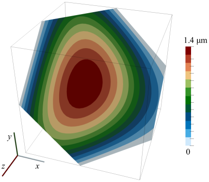
(a) Magnitude of the manufactured displacement solution

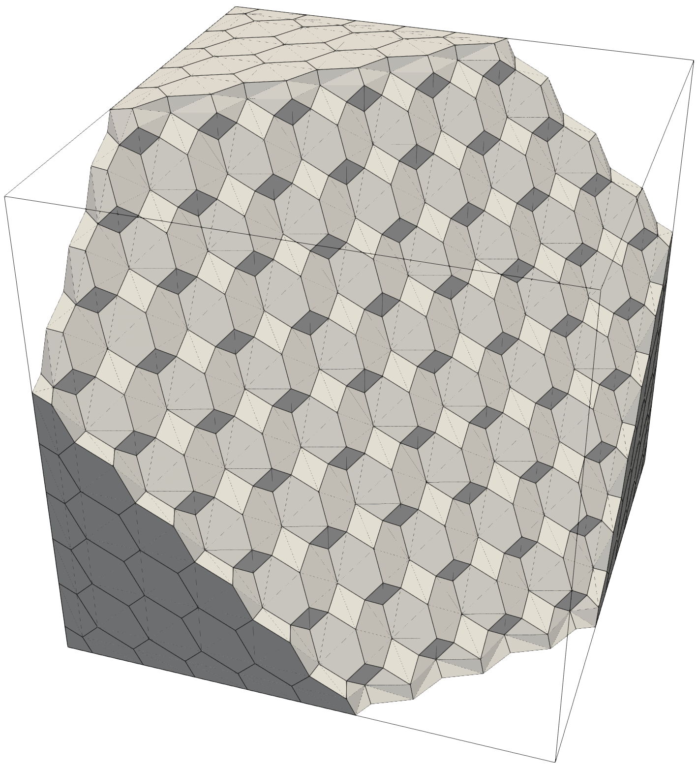
(b) Regular polyhedral mesh with $1\,000$ cells

Figure 2: A cut plane through the cube case geometry showing the magnitude of the manufactured displacement solution (left) and a polyhedral mesh (right). The cut plane passes through the centre of the cube and has the unit normal $\bm{n}=(\nicefrac{{1}}{{\sqrt{3}}}\quad\nicefrac{{1}}{{\sqrt{3}}}\quad\nicefrac{{1}}{{\sqrt{3}}})$.

The manufactured displacement solution is applied at the domain’s boundaries (prescribed displacements), and inertial effects are neglected. Four mesh types are examined: (i) regular tetrahedra, (ii) regular polyhedra (shown in Figure 2(b)), (iii) regular hexahedra, and (iv) distorted hexahedra. The second coarsest meshes are shown in Appendix D. The tetrahedral meshes are created using Gmsh [46], while the polyhedral meshes are created by converting the tetrahedral meshes to their dual polyhedral representations using the OpenFOAM polyDualMesh utility. The regular hexahedral meshes are created using the OpenFOAM blockMesh utility, and the distorted hexahedral meshes are created by perturbing the points of the regular hexahedra by a random vector of magnitude less than 0.3 times the local minimum edge length. Starting from an initial mesh spacing of $0.04$ m, six meshes of each type are created by successively halving the spacing. The cell numbers for the hexahedral and polyhedral meshes are 125, $1\,000$, $8\,000$, $64\,000$, $512\,000$, and $4\,096\,000$, while the tetrahedral mesh cell counts are 384, $4\,374$, $41\,154$, $355\,914$, $2\,958\,234$, and $24\,118\,074$. For the same average cell width, the cell counts show that the tetrahedral meshes have more cells by a factor of 3 to 6.

Figure 3(a) shows the displacement magnitude discretisation errors ($L_{2}$ and $L_{\infty}$) as a function of the average cell width for the four mesh types (tetrahedral, polyhedral, regular and distorted hexahedral), while Figure 3(b) shows the corresponding order of accuracy plots. For ease of interpretation, the symbol shapes in the figures have been chosen to correspond to the cell shapes: a triangle for tetrahedra, a pentagon for polyhedra, a square for regular hexahedra, and a diamond for distorted hexahedra. The maximum ($L_{\infty}$) and average ($L_{2}$) displacement discretisation errors are seen to reduce at an approximately second-order rate for all mesh types, except for the $L_{2}$ error on the hexahedral meshes, which is approximately 2.3 on the finest grid. The distorted hexahedral meshes show the largest average and maximum errors but still approach second-order accuracy as the element spacing decreases.

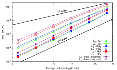
(a) Displacement magnitude discretisation errors

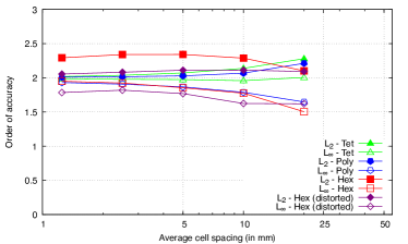
(b) Displacement discretisation error order of accuracy

Figure 3: Manufactured solution cube case: the accuracy and order of accuracy for displacement magnitude

The predicted $\sigma_{xx}$ stress distribution for a hexahedral mesh with $512\,000$ cells is shown in Figure 4(a). The corresponding cell-wise $\sigma_{xx}$ error distribution is shown in Figure 4(b). The errors of greatest magnitude ($43$ kPa) occur at the boundaries, corresponding to where the local truncation error is higher.

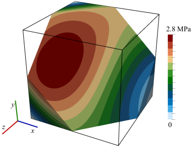
(a) Predicted $\sigma_{xx}$ stress distribution

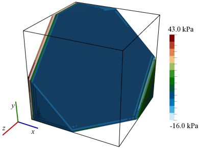
(b) Cell-wise $\sigma_{xx}$ error distribution

Figure 4: Manufactured solution cube case: the predicted $\sigma_{xx}$ stress distribution on a cut-plane for the regular hexahedral mesh with $512\,000$ cells (left).

The discretisation errors in the stress magnitude as a function of cell size are shown in Figure 5(a), and the order of accuracy in Figure 5(b). The order of accuracy for the average ($L_{2}$) stress error is seen to be approximately 1.5 for the hexahedral and polyhedral meshes. In contrast, the average stress error order for the tetrahedral and distorted hexahedral meshes is 1. Similarly, the maximum ($L_{\infty}$) stress order of accuracy is seen to approach 1 for all mesh types. Unlike for the displacements, the greatest stress errors are seen in the tetrahedral rather than the distorted hexahedral meshes; however, the greatest stress maximum errors occur in the distorted hexahedral meshes.

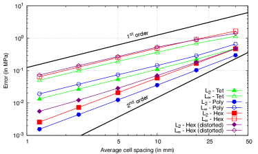
(a) Stress magnitude discretisation errors

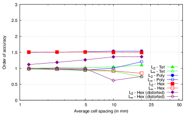
(b) Stress discretisation error order of accuracy

Figure 5: Manufactured solution cube case: the accuracy and order of accuracy for stress magnitude

The presented results agree with the theory: the least squares gradient scheme should be at least first-order accurate for random grids, with greater than first-order accuracy on regular grids due to local truncation error cancellations. In addition, the displacement predictions should be at least second-order accurate on all grid types as long as the gradient scheme achieves at least first-order accuracy.

Case 2: Spherical Cavity in an Infinite Solid Subjected to Remote Stress

This classic 3-D problem consists of a spherical cavity with radius $a=0.2$ m (Figure 6) in an infinite, isotropic linear elastic solid ($E=200$ GPa, $\nu=0.3$). Far from the cavity, the solid is subjected to a tensile stress $\sigma_{zz}=T=1$ MPa, with all other stress components zero.

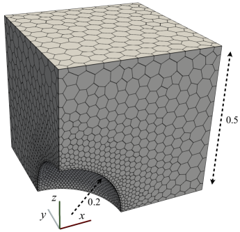
(a) Polyhedral mesh with $4\,539$

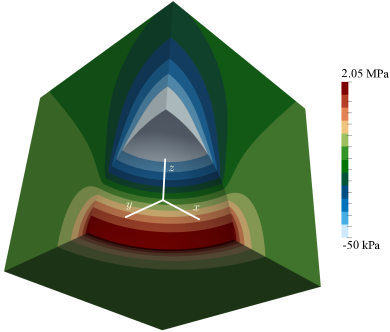
(b) Axial ($zz$) stress distribution on the mesh with $1\,614\,261$ cells

Figure 6: Spherical cavity case

The analytical expressions for the stress, derived by Southwell and Gough [47], and displacement, derived by Goodier [48], are given in Appendix E. The problem is characterised by a localised stress concentration near the cavity on the plane perpendicular to the loading, which drops off rapidly away from the cavity.

The computational solution domain is taken as one-eighth of a $1\times 1\times 1$ m cube aligned with the Cartesian axes, with one corner at the centre of the sphere. The problem is axisymmetric but is analysed here using a 3-D domain to allow a graded unstructured polyhedral mesh to be assessed. The analytical tractions are applied at the far boundaries of the domain to mitigate the effects of finite geometry. The average cell sizes at the cavity surfaces are 100, 50, 25, 12.5, 6.25, and 3.125 mm, and the corresponding cell counts are 976, $4\,552$ (Figure 6), $29\,611$, $213\,100$, $1\,614\,261$. Initially, unstructured tetrahedral meshes were generated using the Gmsh meshing utility [46], followed by conversion to their dual polyhedral representations using the OpenFOAM polyDualMesh utility.

Figure 6(b) shows the predicted axial ($zz$) stress field on the mesh with $1\,614\,261$ cells. The predicted mean ($L_{2}$) and maximum ($L_{\infty}$) displacement and axial stress discretisation errors as a function of the average cell width are presented in Figure 7. The mean and maximum displacement errors are seen to reduce at an approximately second-order rate, while the stress errors are seen to reduce at a first-order rate. As seen in the previous case, the results agree with the theoretical expectations for unstructured (irregular) meshes.

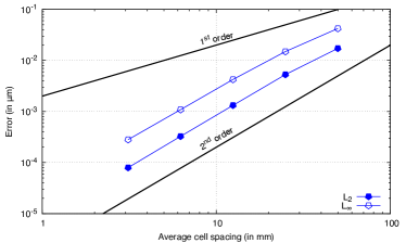
(a) Displacement magnitude discretisation errors

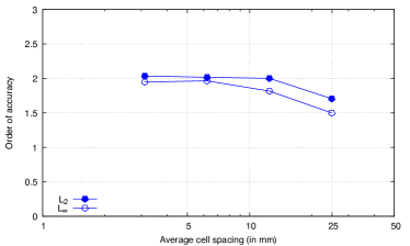
(b) Displacement discretisation error order of accuracy

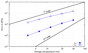
(c) Axial ($zz$) stress discretisation errors

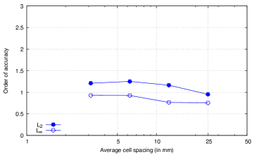
(d) Axial ($zz$) stress discretisation error order of accuracy

Figure 7: Spherical cavity discretisation errors as a function of the average cell spacing

Case 3: Out-of-plane bending of an elliptic plate

This 3-D, static, linear elastic test case (Figure 8) consists of a thick elliptic plate (0.6 m thick) with a centred elliptic hole, with the inner and outer ellipses given as

$$\left(\frac{x}{2}\right)^{2}+\left(\frac{y}{1}\right)^{2}=1$$ inner ellipse (46)

$$\left(\frac{x}{3.25}\right)^{2}+\left(\frac{y}{2.75}\right)^{2}=1$$ outer ellipse (47)

The case has been described by the National Agency for Finite Element Methods and Standards (NAFEMS) [49] and analysed using finite volume procedures by Demirdžić et al. [50] and Cardiff et al. [51]. Unlike the previous cases, this case features significant bending, which is known to slow the convergence of segregated solution procedures [51]. Symmetry allows one-quarter of the geometry to be simulated. A constant pressure of 1 MPa is applied to the upper surface, and the outer surface is fully clamped. The mechanical properties are: $E=210$ GPa, $\nu=0.3$. Six successively refined hexahedral meshes are used, with cell counts of 45, 472 (Figure 8), $4\,140$, $34\,968$, $287\,280$ and $2\,438\,242$.

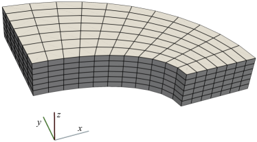
Figure 8: Elliptic Plate geometry and mesh containing 472 hexahedral cells

The prediction for the equivalent (von Mises) stress in the domain are shown in Figure 9(a), and the values along the line $r=\sqrt{x^{2}+y^{2}}=2.1$ m, $z=0.3$ m are shown in Figure 9(b). The results from the finest grid in Demirdžić et al. [50] are given for comparison, where good agreement is seen; the small offset between the finest mesh predictions and those from Demirdžić et al. [50] are likely due to errors introduced when extracting the Demirdžić et al. [50] results using WebPlotDigitizer [52]. The sample values have been calculated by generating 40 uniformly spaced angles between 0 and $\nicefrac{{\pi}}{{2}}$ along the line, finding the cell of each sampled point, and extrapolating from the cell-centred value using the field gradient.

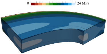
(a) Equivalent stress distribution for the mesh with $2\,438\,242$ cells. The deformation is scaled by $1\,000$ and a translucent line indicates the outline of the undeformed geometry

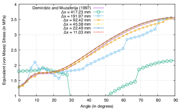
(b) Equivalent stress along the line $r=2.1$, $z=0.3$ m

Figure 9: Equivalent (von Mises) stress distribution in the elliptic plate

Case 4: Inflation of an idealised ventricle

Inflation of an idealised ventricle (Figure 10) was proposed by Land et al. [53] as a benchmark problem for cardiac mechanics software. The case is 3-D, static, with finite hyperelastic strains. The initial geometry is defined as a truncated ellipsoid:

$$x=r_{s}\sin(u)\cos(v),\quad y=r_{s}\sin(u)\sin(v),\quad z=r_{l}\cos(u)$$ (48)

where on the inner (endocardial) surface $r_{s}=7$ mm, $r_{l}=17$ mm, $u\in\left[-\pi,-\arccos\left(\frac{5}{17}\right)\right]$ and $v\in\left[-\pi,\pi\right]$, while on the outer (epicardial) surface $r_{s}=10$ mm, $r_{l}=20$ mm, $u\in\left[-\pi,-\arccos\left(\frac{5}{20}\right)\right]$ and $v\in\left[-\pi,\pi\right]$. The base plane $z=5$ mm is implicitly defined by the ranges for $u$. The hyperelastic material behaviour is described by the transversely isotropic constitutive law proposed by Guccione et al. [54] law, where the parameters are $C=10$ kPa, $c_{f}=c_{t}=c_{fs}=1$; the specified parameters produce isotropic behaviour. The benchmark specifies an incompressible material; in the current work, incompressibility is enforced weakly using a penalty approach, where the bulk modulus parameter is chosen to be two orders of magnitude greater ($\kappa=1000$ kPa) than the greatest shear modulus parameter. A pressure of 10 kPa is applied to the inner surface over 100 equal load increments, and the base plane is fixed. The geometry is meshed using a revolved, structured approach and is predominantly composed of hexahedra, with prism cells forming the apex. The OpenFOAM utilities blockMesh and extrudeMesh are used to create the meshes. Four successively refined meshes are examined: $1\,620$ (shown in Figure 10(a)), $12\,960$, $103\,680$, and $829\,440$ cells. The case can be simulated as 2-D axisymmetric but is simulated here using the full 3-D geometry.

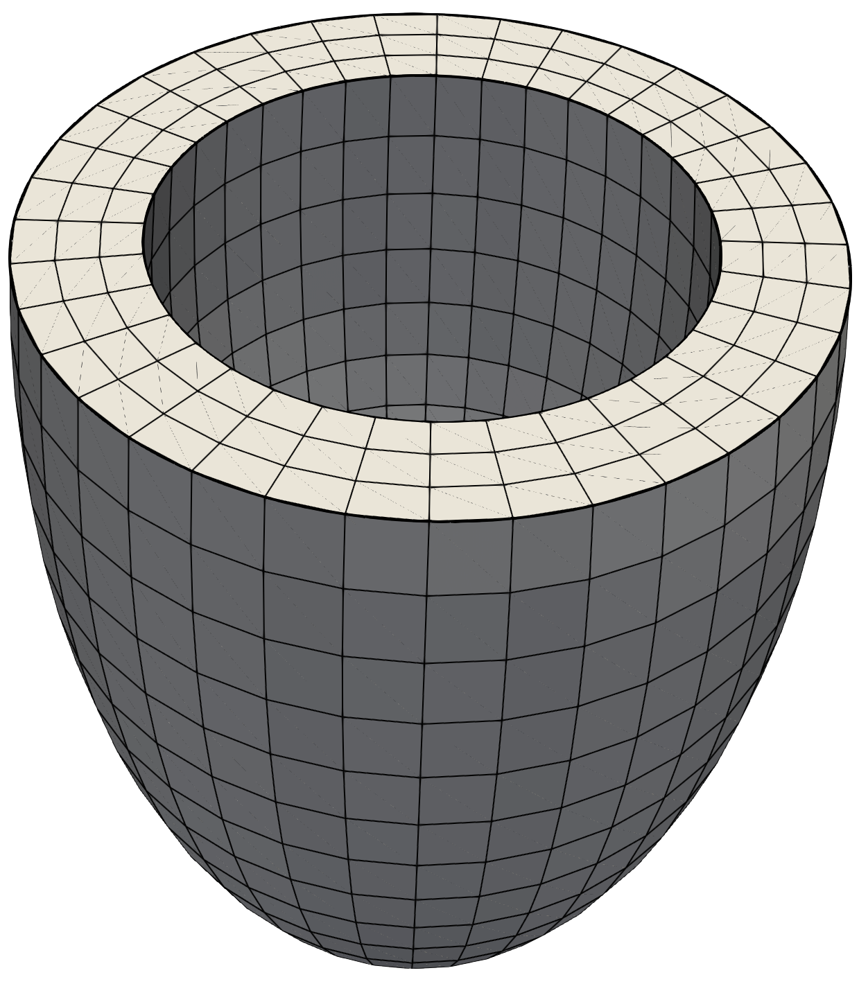
(a) Ventricle undeformed geometry, showing the mesh with 1,620 cells

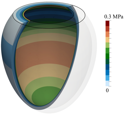
(b) Cross-section showing the equivalent (von Mises) stress distribution for the mesh with 829,440 cells

Figure 10: Idealised ventricle case

The equivalent (von Mises) stress at full inflation is shown for the mesh with 829,440 cells in Figure 10(b), where the high stresses on the inner (endocardial) surface quickly drop off through the wall thickness towards the outer (endocardial) surface. The predicted deformed configuration of the ventricle wall midline is shown in Figure 11, where a side-by-side comparison is given with the round-robin benchmark results from Land et al. [53]. The predictions are seen to become quickly mesh-independent and fall within the benchmark ranges.

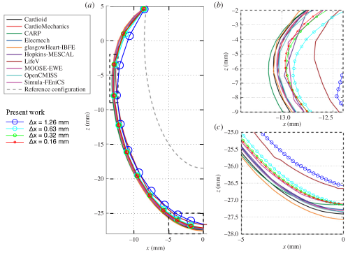
Figure 11: Idealised ventricle: predictions for the four meshes from the present work overlaid on the round-robin predictions from Land et al. [53]

Case 5: Cook’s membrane

Cook’s membrane (Figure 12) is a well-known bending-dominated benchmark case used in linear and non-linear analysis. The 2-D plane strain tapered panel (trapezoid) is fixed on one side and subjected to uniform shear traction on the opposite side. The vertices of the trapezoid (in mm) are (0, 0), (48, 44), (48, 60), and (0, 44).

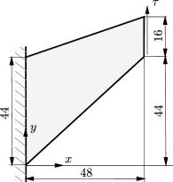
(a) Case geometry and dimensions (in mm)

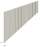
(b) Quadrilateral mesh with 144 cells

Figure 12: Cook’s membrane case geometry and mesh

The current work considers three forms of the problem:

1. Small strain, linear elastic [55, 56]: $E=70$ MPa, $\nu=1/3$, and $\tau=6.25$ kPa.

2. Finite strain, neo-Hookean hyperelastic [57]: $E=1.0985$ MPa, $\nu=0.3$, and $\tau=62.5$ kPa.

3. Finite strain, neo-Hookean hyperelastoplastic [58, 56, 59]: $E=206.9$ MPa, $\nu=0.29$, $\sigma_{y}(\bar{\varepsilon}_{p})=0.45+0.12924\bar{\varepsilon}_{p}+(0.715-0.45)(1-e^{-16.93\bar{\varepsilon}_{p}})$ MPa, and $\tau=312.5$ kPa.

where $E$ is the Young’s modulus, $\nu$ is the Poisson’s ratio, $\tau$ is the prescribed shear traction, and $\sigma_{y}(\bar{\varepsilon}_{p})$ is the yield strength, which is a function of the equivalent plastic strain $\bar{\varepsilon}_{p}$. Eight successively refined quadrilateral meshes are considered, where the cell counts are 9, 36, 144 (Figure 12(b)), 576, $2\,304$, $9\,216$, $36\,864$, and $147\,456$. The problem is solved quasi-statically, and there are no body forces. The linear elastic case is solved in one loading increment, whereas the hyperelastic and hyperelastoplastic cases use 30 equally sized loading increments.

Figure 13 shows the predicted equivalent stress distribution on the mesh with $36\,842$ cells for linear elastic, hyperelastic and hyperelastoplastic cases. The stress distribution is consistent with bending, with regions of high stress near the upper and lower surfaces and a line of relatively unstressed material in the centre. The greatest equivalent stresses occur at the top-left corner and the lower surface in all versions of the case. In the hyperelastoplastic case, almost the entire domain is plastically yielding with only a small thin region remaining elastic, indicated by the blue line in Figure 13(c).

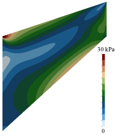
(a) Linear elastic case

(b) Hyperelastic case

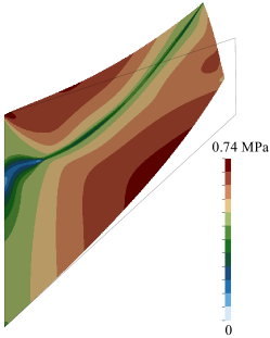
(c) Hyperelastoplastic case

Figure 13: Equivalent (von Mises) stress distribution for the three Cook’s membrane cases using the mesh with $36\,842$ cells

Figure 14 compares the predicted vertical displacement at the reference point as a function of the average cell widths with results from the literature and finite element software Abaqus (element code C3D8). The reference point is taken as the top right point – $(48,60)$ mm – in the elastic and hyperelastoplastic cases, while it is taken as the midway point of the loading surface – $(48,52)$ mm – in the hyperelastic case.

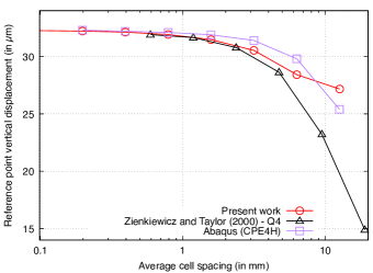
(a) Linear elastic case

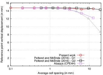
(b) Hyperelastic case

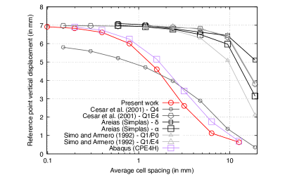
(c) Hyperelastoplastic case

Figure 14: Cook’s membrane vertical displacement predictions at the reference point as a function of the average cell width. Comparisons are given with the results from the literature [55, 57, 58, 56]

The results shown for the hyperelastoplastic case were generated using the segregated solution procedure as the Jacobian-free Newton-Krylov approach diverged for six of the eight mesh densities, as discussed further in Section 4.2.

Case 6: Vibration of a 3-D Cantilevered Beam

This 3-D, dynamic, finite strain case geometry consists of a $2\times 0.2\times 0.2$ m cuboid column and was proposed in its initial form by Tuković and Jasak [60]. A sudden, constant traction $\bm{T}=\left(50,50,0\right)$ kPa is applied to the upper surface. A neo-Hookean hyperelastic material is assumed with $E=15.293$ MPa, $\nu=0.3$ and density $\rho=1000$ kg m^-3, while the area $A=0.04$ m² and the second moment of area $I=\nicefrac{{1}}{{7\,500}}$ m⁴. The geometric and material parameters were chosen for the first natural frequency to be 1 Hz in the small strain limit. The magnitude of the applied traction is chosen here to test the robustness of the solution procedures when large rotations and strains are present. Four succesively refined hexahedral meshes are generated using the OpenFOAM blockMesh utility, with cell counts of 270, $2\,160$, $17\,280$ and $138\,240$. The time step size is 1 ms, and the total period is 1 s.

The deformed configuration of the beam at six time steps is shown in Figure 15(a) for the mesh with $2\,160$ cells, where the upper surface is seen to drop below the horizontal from approximately t = 0.2 s to 0.32 s. The corresponding displacement magnitude of the centre of the upper surface of the beam vs time is shown in Figure 15(b), where the predictions are seen to converge to the results from finite element software Abaqus (element code C3D8) using the $138\,240$ mesh.

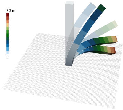
(a) Displacement magnitude for t = $\left\{0,\,0.1,\,0.2\right\}$ s (translucent) and t = $\left\{0.3,\,0.4,\,0.5\right\}$ s (opaque) for the mesh with $138\,240$ cells

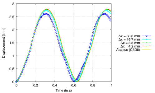
(b) Displacement magnitude of the centre of the upper surface of the beam vs time

Figure 15: Deflection of a 3-D Cantilevered Beam

Case 7: Elastic plate behind a rigid cylinder

The final test case, introduced by Turek and Hron [61], extends the classic flow around a cylinder in a channel problem [62] into a well-established fluid-solid interaction benchmark. The FSI3 variant of the case examined here (Figure 16) consists of a horizontal channel (0.41 m in height, 2.5 m in length) with a rigid cylinder of radius 0.05 m, where the cylinder centre is 0.2 m from the bottom and inlet (left) boundaries. A parabolic velocity is prescribed at the inlet velocity with a mean value of 2 m/s. A St. Venant-Kirchhoff hyperelastic plate ($E=5.6$ MPa, $\nu=0.4$) of 0.35 m in length and 0.02 m in height is attached to the right-hand side of the rigid cylinder. The fluid model is assumed to be isothermal, incompressible, and laminar and adopts the segregated PIMPLE solution algorithm. The fluid’s kinematic viscosity is 0.001 m²/s and density is 1000 kg m^-3, while the solid’s density is $10\,000$ kg m^-3. The interface quasi-Newton coupling approach with inverse Jacobian from a least-squares model [63] is employed for the fluid-solid interaction coupling. The fluid-solid interface residual is reduced by four orders of magnitude within each time step. Further details of the fluid-solid interaction procedure are found in Tuković et al. [11]. Three successively refined quadrilateral meshes are employed: The fluid region meshes have $1\,252$, $5\,008$, and $20\,032$ cells, while the solid region meshes have 156, 624 and $2\,496$ cells. The total simulation time is 20 s, and the time-step size is 0.5 ms.

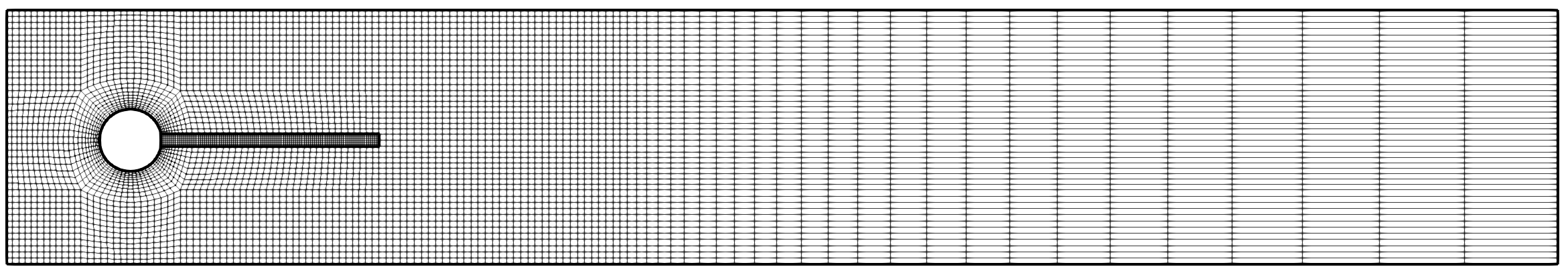
(a) Mesh containing $5\,336$ cells in the fluid region and 630 cells in the solid region

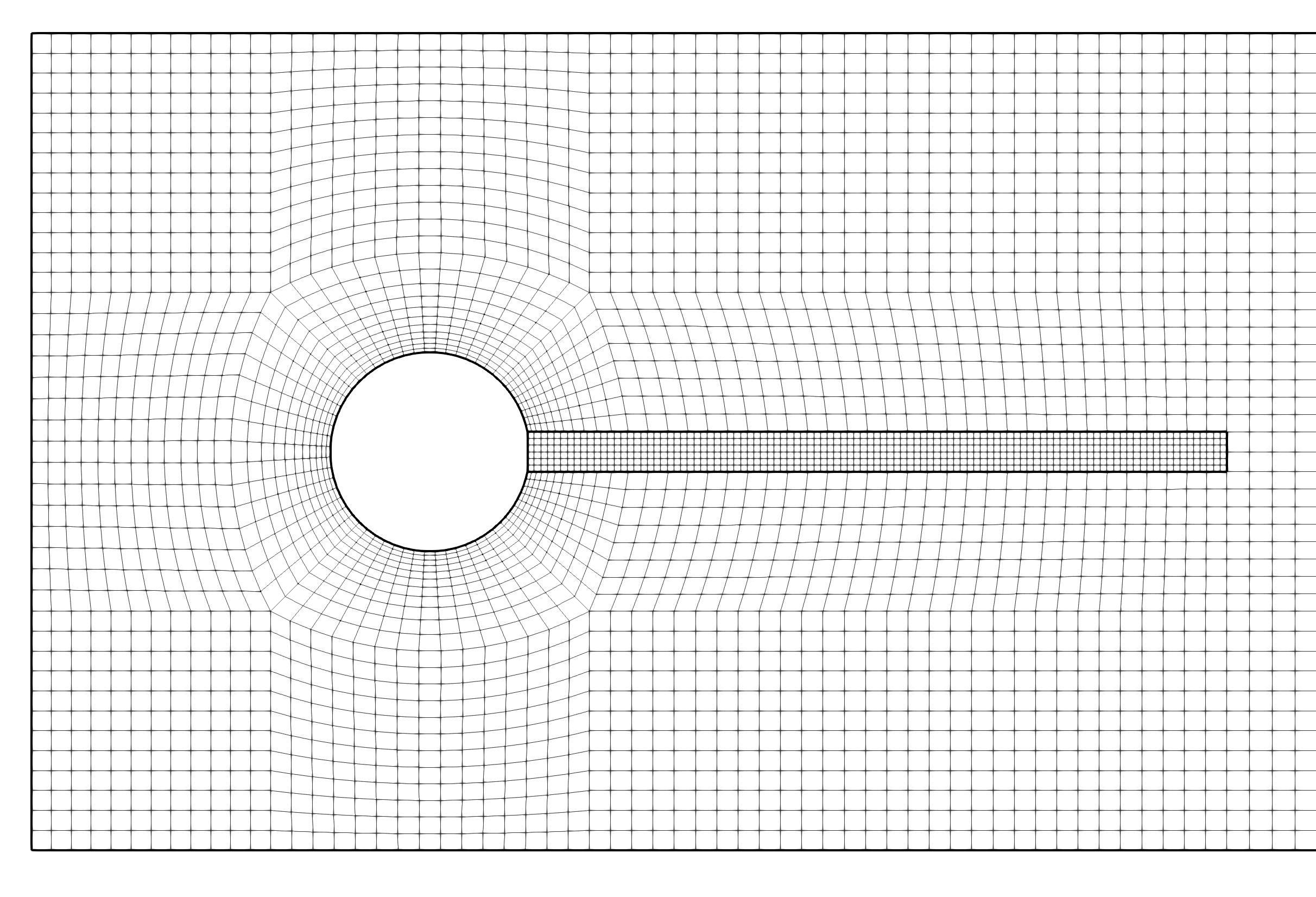
(b) Close-up of the mesh around the plate

Figure 16: Elastic plate behind a rigid cylinder case geometry and mesh

Figure 17 shows the velocity field in the fluid region and displacement magnitude in the solid region at $t=4.42$ s, corresponding to a peak in the vertical displacement of the plate free-end oscillation. The fluid is seen to accelerate as it passes the cylinder, with regular vortices being thrown off the plate, causing it to oscillate.

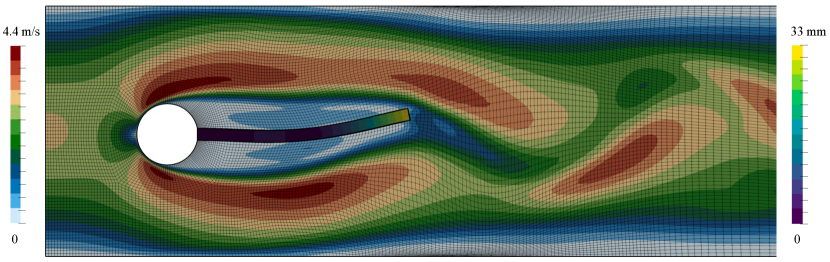
Figure 17: Elastic plate behind a rigid cylinder case results at $t=20$ s for the mesh with $20\,032$ cells in the fluid region and $2\,496$ in the solid region. The velocity magnitude is shown in the fluid region, while the displacement magnitude is shown in the solid region.

The predicted mean, amplitude and frequency of the vertical and horizontal displacement of the end of the plate are seen to approach the results from Turek and Hron [61] in Table 4.1. As directed in Turek and Hron [61], the maximum and minimum values for the last period are used to calculate the mean and amplitude:

$$\text{mean}=\frac{1}{2}(\text{max}+\text{min}),\quad\quad\text{amplitude}=\frac{1}{2}(\text{max}-\text{min})$$ (49)

while the frequency is calculated as the inverse of the period.

Mesh (number of fluid and solid cells)	$u_{x}$ (in mm)	$u_{y}$ (in mm)
1 ($1252$ + $156$)	$-0.10\pm 0.03\,[58.82]$	$1.60\pm 0.00\,[5.78]$
2 ($5008$ + $624$)	$-2.10\pm 2.02\,[10.42]$	$1.44\pm 29.68\,[5.59]$
3 ($20032$ + $2496$)	$-2.46\pm 2.30\,[10.75]$	$1.46\pm 32.63\,[5.68]$

Turek and Hron [61] & $-2.69\pm 2.53\,[10.9]$ $1.48\pm 34.38\,[5.3]$

Table 1: Predicted oscillations (mean $\pm$ amplitude $[$frequency$]$) of the free end of the plate. Note that large-scale plate oscillations in mesh 1 (coarsest mesh) die out within the first 10 s.

4.2 Resource Requirements and Robustness

This section compares resource requirements and the robustness of the Jacobian-free Newton-Krylov and segregated approaches on the cases presented in Section 4.1. Specifically, time and memory requirements are analysed, and whether the solution converged for all meshes and loading steps. In all cases, the Jacobian-free Newton-Krylov approach used the GMRES linear solver with the direct LU preconditioner for 2-D and the Hypre BoomerAMG multigrid preconditioner for 3-D, unless stated otherwise. A restart value of 30 is used for the GMRES solver, where the loose variant of the GMRES solver is used, which retains a small number of extra solution vectors across restarts (2 in this case). In contrast, the segregated approach used the conjugate gradient linear solver and the incomplete Cholesky preconditioner with no infill – equivalent to ILU(0). Time and memory requirements are implementation and hardware-specific; nonetheless, it is insightful to see the relative performances of the Jacobian-free Newton-Krylov and segregated approaches on the same hardware and within the same implementation framework. Clock times and memory usage (measured with the GNU time utility) were generated using a Mac Studio with an M1 Ultra CPU on one core, where the code was built with the Clang compiler (version 16.0.0). Examination of multi-CPU-core parallelisation is left to Section 4.5.

Table 4.2 lists the wall clock times (time according to a clock on the wall) and maximum memory usage for all cases and all meshes, where diverged cases are indicated by the symbol ${\dagger}$. Figure 19(a) plots the corresponding speedup on all cases as a function of the number of degrees of freedom, where the speedup is defined as the segregated clock time divided by the Jacobian-free Newton-Krylov clock time. The number of degrees of freedom is $2\times$ the cell count in 2-D cases and $3\times$ in 3-D cases, except in the fluid-solid interaction case where the fluid domain has three degrees of freedom (two velocity components and pressure) in 2-D. Speedup is only calculated for clock times greater than 2 seconds to avoid the comparison of small numbers. In all cases where convergence was achieved, the Jacobian-free Newton-Krylov approach was faster (speedup $>1$), with speedups of one or two orders of magnitude in many cases. Additionally, it can be observed from Figure 19(a) that the speedup increases as the number of degrees of freedom increases. The largest speedup was 341 on the sixth mesh ($9\,216$ cells) of the membrane i (2-D, linear elastic) case, while the lowest speed was 1 and occurred in the manufacctured solution coarser meshes.

Table 2: Execution times (rounded to the nearest second) and maximum memory usage for Jacobian-free Newton-Krylov (JFNK) and segregated methods (rounded to the nearest MB). ${\dagger}$ indicates the solver diverged.

& 976 0 103 1 90 Cavity $4\,552$ 1 204 1 143 3-D, static $29\,611$ 6 982 9 543 linear elastic $213\,100$ 87 $5\,804$ 135 $1\,620$ $1\,614\,261$ $1\,265$ $27\,173$ $2\,367$ $9\,017$ Elliptic Plate $45$ 0 75 0 65 3-D static $472$ 0 80 1 69 linear elastic $4\,140$ 0 131 2 109 $34\,968$ 8 709 35 415 $287\,280$ 107 $3\,852$ 475 $1\,497$ $2\,438\,242$ $1\,073$ $22\,957$ $7\,176$ $7\,021$ Ventricle $1\,620$ 52 150 ${\dagger}$ 123 3-D, static $12\,960$ 608 595 ${\dagger}$ 415 hyperelastic $103\,680$ $11\,893$ 2350 ${\dagger}$ 1999 $829\,440$ $118\,944$ 7957 ${\dagger}$ 5589 Membrane i 9 0 76 0 65 2-D static 36 0 76 1 65 linear elastic 144 0 77 1 66 576 0 81 1 73 $2\,304$ 0 99 1 81 $9\,216$ 0 174 9 143 $36\,864$ 2 606 67 422 $147\,456$ 9 $1\,605$ 532 $1\,384$ Membrane ii 9 0 76 1 65 2-D, static, 36 0 76 2 65 hyperelastic 144 0 77 7 65 576 0 82 52 67 $2\,304$ 2 106 503 89 $9\,216$ 8 213 $2\,725$ 188 $36\,864$ 37 686 $1\,795$ 469 $147\,456$ 170 $2\,118$ $15\,573$ 910 Membrane iii 9 0 76 2 66 2-D, static, 36 1 77 6 66 hyperelastoplastic 144 ${\dagger}$ 79 29 67 576 ${\dagger}$ 83 167 73 $2\,304$ ${\dagger}$ 103 894 102 $9\,216$ ${\dagger}$ 218 $6\,936$ 262 $36\,864$ ${\dagger}$ 813 $57\,753$ $1\,217$ $147\,456$ ${\dagger}$ $1\,832$ $522\,811$ $3\,216$ Cantilever $270$ 12 85 11 73 3-D, dynamic $2\,160$ 87 166 93 94 hyperelastic $17\,280$ $1\,028$ 739 $1\,459$ 591 $138\,240$ $12\,156$ $5\,791$ ${\dagger}$ $1\,838$ FSI $1\,252$ + 156 $3\,591$ 773 $5\,883$ 869 2-D, dynamic, $5\,008$ + 624 $25\,920$ 911 $43\,365$ 884 hyperelastic $20\,032$ + $2\,496$ $154\,938$ 908 $199\,143$ 865

Figure 18(b) shows the relative memory usage, defined here as the maximum memory usage of the Jacobian-free Newton-Krylov approach divided by that of the segregated approach. The relative memory usage is close to unity for coarse meshes (less than $10^{4}$ degrees of freedom), but shows a general increasing trend beyond this. The maximum value for relative memory was 3.6 and occurred in the second-finest mesh for the spherical cavity case. The variations in the relative memory trends between cases can likely be attributed to the variable memory usage of the GMRES linear solver in the Jacobian-free Newton-Krylov, where the number of stored directions can vary depending on the ease of convergence. In addition, the memory usage of the multigrid preconditioner can vary depending on the geometry and cell types. The effect of the preconditioner and linear solver settings are examined further in Section 4.3.

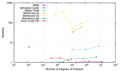
(a) Speedup

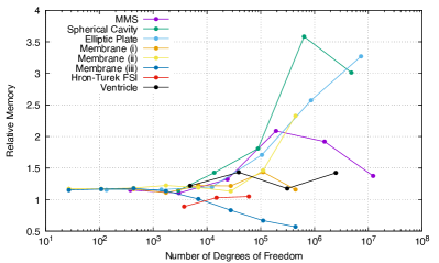
(b) Relative memory

Figure 18: The speedup (segregated clock time divided by the Jacobian-free Newton-Krylov clock time) and relative memory usage (segregated maximum memory usage divided by the Jacobian-free Newton-Krylov maximum memory usage) as a function of degrees of freedom

Regarding robustness, the Jacobian-free Newton-Krylov approach converged in all cases bar one, requiring less than five outer Newton iterations on average in all converged cases. The only case where the Jacobian-free Newton-Krylov approach failed to converge was for the membrane iii problem, the only elastoplastic case examined. For the failed meshes, approximately 80% of the total load was reached before the linear solver diverged. The cause of this divergence is likely related to the proposed compact preconditioner matrix – which is formulated based on small elastic strains – being a poor approximation of the true Jacobian for large plastic strains. Interestingly, convergence problems were not encountered in the hyperelastic cases (membrane ii, ventricle, cantilever, fluid-solid interaction), demonstrating that the proposed compact linear elastic preconditioner matrix is suitable for such large strain, large rotation hyperelastic cases. In contrast, the segregated approach – which uses the same matrix – had no problems with the elastoplastic case (membrane iii) but failed to converge on two of the hyperelastic cases (ventricle, cantilever). In both cases where the segregated approach failed, large elastic strains and large rotations were observed, and the segregated solver failed in the early time steps. It is interesting to note that the same linear elastic preconditioner matrix works well with the Jacobian-free Newton-Krylov approach for hyperelastic cases but not for the segregated approach, while the opposite is true for elastoplastic cases.

Regarding geometric dimension, the same general trends are observed in 2-D and 3-D, with no major distinctions in behaviour. The same can be said for geometric nonlinearity (small strain vs. large strain) with similar speed-ups for both linear elastic and hyperelastic cases. One observation worth highlighting is the lower speedup seen for the method of manufactured solutions case (3-D, linear elastic): a possible explanation is that the segregated approach has previously been seen to be efficient on geometry with low aspect ratios (ratio of maximum to minimum dimensions) and minimal bending deformation; in this case, the aspect ratio is at its minimum (unity) and bending deformation is localised. In contrast, in the other 3-D linear elastic cases (elliptic plate, membrane i), the aspect ratios are greater than unity and more widespread bending is present, and the segregated approach performs worse relative to the Jacobian-free Newton-Krylov approach.

4.3 Effect of the Preconditioner Choice

This section examines the effect of preconditioning strategy on the performance of the Jacobian-free Newton Krylov approach. Three choices of preconditioning procedure are compared:

• LU - The MUltifrontal Massively Parallel sparse direct Solver (MUMPS) [43, 44] LU decomposition direct solver. A direct solver is expected to be the more robust but may suffer from excessive time and memory requirements for larger numbers of unknowns.

• ILU($k$) - Incomplete LU decomposition with $k$ fill-in. ILU($k$) is expected to have lower memory requirements than the LU direct solver but at the expense of robustness. As the system of unknowns becomes larger, the number of ILU($k$) iterations is expected to increase. As the fill-in factor $k$ increases, ILU($k$) approaches the robustness of a LU direct solver. In the current section, $k=5$ for all cases examined.

• Algebraic multigrid - The Hypre Boomerang [42] parallelised multigrid preconditioner. Multigrid approaches have the potential to offer superior performance than other methods for larger problems, with near linear scaling of time and memory requirements.

An additional consideration when selecting a preconditioner is its ability to scale in parallel as the number of CPU cores increases. From this perspective, the iterative approaches (ILU($k$) and multigrid) are expected to show better parallel scaling than direct methods (LU), a point that is briefly examined in Section 4.5.

The preconditioning approaches are compared in three cases: membrane i (2-D, linear elastic), elliptic plate (3-D, linear elastic), and idealised ventricle (3-D, hyperelastic). Figure 19 compares the clock times and maximum memory requirements for the three preconditioning approaches as a function of degrees of freedom. Examining the clock times, the LU preconditioner is seen to be faster for all meshes in the membrane i and idealised ventricle cases, while the multigrid approach is faster for all meshes in the elliptic plate cases. The LU approach was found to be up to $5.4\times$ faster in the membrane i case than the multigrid approach, and $1.8\times$ faster in the idealised ventricle case. In contrast, the multigrid was up to $1.4\times$ faster than the LU approach in the elliptic plate case. The ILU(5) approach is seen to be slowest in all cases, in addition, the ILU(5) approach diverged on the idealised ventricle finest mesh; lower values of fill-in $k$ were found to cause divergence to occur earlier in the idealised ventricle case.

Regarding memory usage, below approximately $50$ k degrees of freedom, the memory usage is the same for all three approaches (approximately $80$ MB), corresponding to the solver’s minimum memory overhead. For greater numbers of degrees of freedom, the LU approach uses the greatest amount of memory for both 3-D cases (idealised ventricle, elliptic plate), while the ILU(5) uses the least. In contrast, the LU approach uses the smallest amount of memory for the 2-D cases (membrane i) examined. The rate of memory increase is seen to be much steeper for the LU approach on the 3-D cases than the multigrid and ILU(5) approaches, with the LU results for the finest meshes not shown as they required more than the maximum available memory (64 GB).

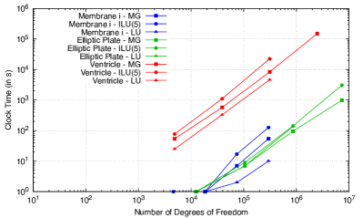
(a) Clock time

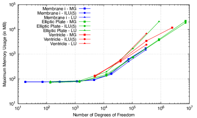
(b) Maximum memory

Figure 19: The clock times and maximum memory usage for three preconditioning approaches (multigrid, ILU(5), and LU) as a function of degrees of freedom

4.4 Effect of Rhie-Chow Stabilisation

This section highlights the impact of the global scaling factor $\alpha$ in the Rhie-Chow stabilisation (Equation 27) on the performance of the proposed Jacobian-free Newton Krylov method. As described in Section 2.3, the stabilisation term is introduced to quell zero-energy modes (oscillations) in the discrete solution, such as checkerboarding. As the amount of stabilisation increases (increasing $\alpha$), these numerical modes are quelled, and the solution stabilises; however, at some point, further increases in the amount of stabilisation reduce the accuracy of the discretisation due to over-smoothing. A less obvious consequence of changing the stabilisation magnitude is its effect on the convergence of the linear solver in the Jacobian-free Newton-Krylov solution procedure. This section examines this effect.

As in the previous section, three cases are used to highlight the effect: membrane i (2-D, linear elastic), elliptic plate (3-D, linear elastic), and idealised ventricle (3-D, hyperelastic). The LU preconditioning method is used for the 2-D membrane i case, while the multigrid approach is used for the two 3-D cases. Figure 20 presents the execution times and the number of accumulated linear solver iterations for three values of global stabilisation factor ($\alpha=\left[0.01,0.1,1\right]$) for several mesh densities. The memory usage is unaffected by the value of $\alpha$ and is hence not shown. From Figure 20(a), the clock time is seen to increase exponentially (linearly on a log-log plot) for all cases and all values of $\alpha$. For all meshes in all three cases, the lowest value of global stabilisation factor ($\alpha=0.01$) – corresponding to the least amount of stabilisation – takes the greatest amount of time to converge, while the largest value of global stabilisation factor ($\alpha=1$) is the fastest to converge. In the membrane i case, the largest value of ($\alpha$) is approximage $1.5\times$ faster than the lowest value of $\alpha$. Nonetheless, the clock time is not a linear function of $\alpha$, and it can be seen that $\alpha=0.1$ requires approximately the same amount of time as $\alpha=1$ in all cases. In terms of robustness, the idealised ventricle cases failed with $\alpha=0.01$, suggesting increasing the stabilisation increases robustness. From Figure 20(b), the accumulated number of linear solver (GMRES) iterations are seen to follow the same trends as the clock times, where $\alpha=0.01$ requires the greatest number of iterations while $\alpha=0.1$ and $\alpha=1$ require approximately the same number of iterations. In all cases, the number of iterations are seen to increase as the number of degrees of freedom increase.

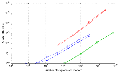
(a) Clock time

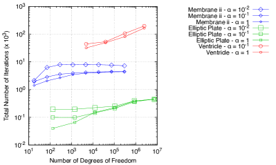
(b) Accumulated linear solver iterations

Figure 20: The clock times and accumulated linear solver iterations for different values of Rhie-Chow global stabilisation factor $\alpha$

4.5 Parallelisation

In this final analysis, the multi-CPU-core parallel scaling performance of the proposed Jacobian-free Newton Krylov method is compared with the segregated approach. A strong scaling study is performed, where the clock time to solve a fixed-size problem is measured as the number of CPU cores is increased. The elliptic plate (3-D, linear elastic) mesh with $2\,438\,242$ cells is chosen for the scaling analysis. Parallelisation adopts the standard OpenFOAM domain decomposition approach, where the mesh is decomposed into one sub-domain for each CPU core. In the current work, the Scotch decomposition approach [64] is employed. The Jacobian-free Newton Krylov approach uses the GMRES linear solver where the performance of the multigrid and LU preconditioners are compared. The segregated approach uses the conjugate gradient solver with the incomplete (zero in-fill – $k=0$) Cholesky preconditioner. The cases are run on the MeluXina high-performance computing system, where each standard computing node contains $2\times$ AMD EPYC Rome 7H12 64c 2.6GHz CPUs with 512 GB of memory. In the current study, the number of CPU cores are varied from 1 to $1\,048$ ($\left[1,2,4,8,16,32,64,128,256,512,1\,048\right]$). In the ideal case, the speedup should double when the number of cores is doubled; in reality, inter-CPU-core communication reduces the parallel scaling efficiency below the ideal.

The clock times from the strong scaling study are shown in Figure 21(a), where the ideal scaling is shown for comparison as a dashed line. Figure 21(b) shows the corresponding speedup, defined as the clock time on one CPU core divided by the clock time on a given number of CPU cores. The Jacobian-free Newton-Krylov approach with the multigrid preconditioner is found to be the fastest by almost an order of magnitude over the segregated approach and the Jacobian-free Newton-Krylov approach with LU preconditioner. The times for the segregated and Jacobian-free Newton-Krylov LU preconditioner approaches using 1, 2, and 4 cores were not recorded due to the excessive times. For all approaches the speedup is seen to increase at an approximately ideal rate up to 128 cores, after which the speedup continues to increase but at a lower rate. At 128 cores (corresponding to one full computing node), the number of cells per core is approximately 19 k; increasing the number of cores beyond 128 likely shows a less than ideal scaling for two reasons: (i) the number of cells per core is becoming small relative to the amount of inter-core communication, and (ii) inter-node communication is likely slower than intra-node communication. The segregated and Jacobian-free Newton-Krylov LU preconditioner approaches produce their fastest predictions at 512 cores, while the Jacobian-free Newton-Krylov multigrid preconditioner approach continues to speedup up to the maximum number of cores tested ($1\,048$), albeit $1\,048$ cores is just $2\times$ faster than 128 cores. At $1\,048$ cores, there is approximately 2.5 k cells per core and the inter-core communication is expected to be significant.

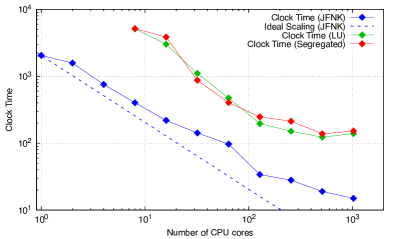
(a) Clock times vs number of CPU cores

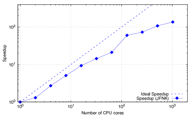
(b) Speedup $S$ vs number of CPU cores

Figure 21: Strong parallel scaling study comparing the performance of the Jacobian-free Newton-Krylov approach using the multigrid and LU preconditioning strategies, and the segregated solution procedure

As a final observation, the effect of hardware can be highlighted by comparing the time required for 1 core when using the multigrid preconditioner: the case required $2\,048$ s on the MeluXina system (EPYC Rome CPU), while it required $988$ s on a Mac Studio (M1 Ultra CPU) system as presented in Section 4.2 – over twice as fast. The difference in performance can be primarily attributed to the unified memory architecture of the M1 Ultra, which provides significantly greater memory bandwidth compared to the DDR4 memory used in the MeluXina compute nodes.

5 Conclusions

A Jacobian-free Newton-Krylov solution algorithm has been proposed for solid mechanics problems discretised using the cell-centred finite volume method. A compact-stencil discretisation of the diffusion term is proposed as the preconditioner matrix, allowing a straightforward extension of existing segregated solution frameworks. The key conclusions of the work are:

• Efficiency of Jacobian-free Newton-Krylov approach: The proposed Jacobian-free Newton-Krylov solution algorithm has been shown to be faster than a conventional segregated solution algorithm for all linear and nonlinear elastic test cases examined. In particular, speedups of one order of magnitude were seen in many cases, with a maximum speedup of 341 in the 2-D linear elastic Cook’s membrane case.

• Additional memory overhead: The Jacobian-free Newton-Krylov approach has been shown to have approximately the same memory requirements as a segregated solution algorithm for less than $10^{4}$ degrees of freedom, but generally increases beyond this. The greatest memory increase was found to be 3.6 and occured in the spherical cavity case. Nonetheless, these differences are likely attributed to the different linear solver and preconditioner used in the Jacobian-free Newton-Krylov approach (GMRESS with multigrid or LU decomposition) compared to the segregated approach (conjugate gradient with zero in-fill Cholesky decomposition).

• Applicability to existing segregated frameworks: By employing a compact-stencil diffusion approximation of the Jacobian as the preconditioner, the proposed Jacobian-free Newton-Krylov approach can be integrated into existing segregated finite volume frameworks with minimal modifications to the existing code base, in particular if existing publicly available Jacobian-free Newton-Krylov solvers (e.g., PETSc) are used.

• Choice of preconditioning approach: It has been shown that the LU direct solver preconditioning approach is faster than multigrid and ILU($k$) approaches for 2-D cases and moderately-sized 3-D problems; however, for larger 3-D problems the multigrid approach is the fastest while also requiring less memory than the direct LU approach. In addition, the multigrid approach is seen to show approximate ideal scaling in a parallel strong scaling study.

• Rhie-Chow stabilisation: The magnitude of the Rhie-Chow stabilisation term is shown to affect the speed and robustness of the Jacobian-free Newton-Krylov approach, where $\alpha=0.1$ and $1$ are seen to outperform $\alpha=0.01$.

• Open access and extensibility: The implementation is made publicly available within the solids4foam toolbox for OpenFOAM to encourage implementation critique, community adoption, and comparative studies, contributing to advancing finite volume solid mechanics simulations.

The presented study highlights the potential of the Jacobian-free Newton-Krylov method in finite-volume solid mechanics simulations, yet several areas for future exploration remain:

1. Enhanced preconditioning for plasticity: While the proposed elastic compact-stencil preconditioning matrix has been shown to perform well in linear and nonlinear elastic scenarios, it fails in cases exhibiting plasticity, where a segregated approach succeeds. Future studies will explore modifications to the compact preconditioning matrix to extend the applicability of the proposed approach to small and large strain elastoplasticity.

2. Incorporation of non-orthogonality in the preconditioner: The current preconditioning matrix does not account for non-orthogonal contributions in distorted meshes. Including these effects in future work could further enhance robustness, particularly for complex geometries.

3. Comparison with full Jacobian approaches: A comparison with a fully coupled Jacobian-based method would provide greater insights into the trade-offs between computational cost, memory usage, and convergence performance. Such a study could highlight the specific advantages of the Jacobian-free Newton-Krylov approach for large-scale, nonlinear problems.

4. Globalisation strategies: The robustness and efficiency of the proposed Jacobian-free Newton-Krylov approach could be improved for nonlinear problems by using a segregated approach as an initialisation phase for each loading step. In its current form, the segregated approach would not be generally suitable as it is less robust on several nonlinear hyperelastic problems; however, modifications such as introducing pseudo-time-stepping (introducing a pseudo-time damping term), may enhance its robustness and suitability for these scenarios.

5. Higher-order discretisations: Future work will explore the application of the proposed linear elastic compact-stencil Jacobian-free Newton-Krylov approach to higher-order finite volume discretisations. Using the same compact-stencil preconditioning matrix for these discretisations could yield efficient and accurate solutions for problems requiring increased fidelity.

6. Development of a monolithic fluid-solid interaction framework: Extending the Jacobian-free Newton-Krylov method to a fully monolithic fluid-solid interaction framework presents a promising avenue. In this approach, both fluid and solid domains would be solved simultaneously using a unified Jacobian-free Newton-Krylov method, potentially improving stability and performance in highly nonlinear coupled problems.

Acknowledgments Technical reviews and insightful comments from Hiroaki Nishikawa of the National Institute of Aerospace, Hampton, VA, USA, are greatly appreciated. This project has received funding from the European Research Council (ERC) under the European Union’s Horizon 2020 research and innovation programme (Grant Agreement No. 101088740). Financial support is gratefully acknowledged from the Irish Research Council through the Laureate programme, grant number IRCLA/2017/45, from Bekaert through the University Technology Centre (UTC phases I and II) at UCD (www.ucd.ie/bekaert), from I-Form, funded by Science Foundation Ireland (SFI) Grant Numbers 16/RC/3872 and RC2302_2, co-funded under European Regional Development Fund and by I-Form industry partners, and from NexSys, funded by SFI Grant Number 21/SPP/3756. Additionally, the authors wish to acknowledge the DJEI/DES/SFI/HEA Irish Centre for High-End Computing (ICHEC) for the provision of computational facilities and support (www.ichec.ie), and part of this work has been carried out using the UCD ResearchIT Sonic cluster which was funded by UCD IT Services and the UCD Research Office.

Appendix A Mechanical Laws

A.1 Linear Elasticity

The definition of engineering stress $\bm{\sigma}_{s}$ for linear elasticity can be given as

$$\bm{\sigma}_{s} = 2\mu\bm{\varepsilon}+\lambda\,\text{tr}\left(\bm{\varepsilon}\right)\textbf{I}$$ (50)

$$= \mu\bm{\nabla}\bm{u}+\mu\left(\bm{\nabla}\bm{u}\right)^{\text{T}}+\lambda\left(\bm{\nabla}\cdot\bm{u}\right)\textbf{I}$$

where $\lambda$ is the first Lamé parameter, and $\mu$ is the second Lamé parameter, synonymous with the shear modulus. The Lamé parameters can be expressed in term of the Young’s modulus ($E$) and Poisson’s ratio $\nu$ as

$$\mu=\frac{E}{2(1+\nu)},\quad\lambda=\frac{E\nu}{(1+\nu)(1-2\nu)}$$ (51)

A.2 St. Venant-Kirchoff Hyperelasticity

The St. Venant-Kirchoff model defines the second Piola–Kirchhoff stress S as

$$\bm{S} = 2\mu\bm{E}+\lambda\,\text{tr}\left(\bm{E}\right)\textbf{I}$$ (52)

where, as before, $\lambda$ is the first Lamé parameter, and $\mu$ is the second Lamé parameter. The Lagrangian Green strain E is defined as

$$\bm{E} = \frac{1}{2}\left(\bm{\nabla}\bm{u}+\bm{\nabla}\bm{u}^{\text{T}}+\bm{\nabla}\bm{u}\cdot\bm{\nabla}\bm{u}^{\text{T}}\right)$$ (53)

The true stress can be calculated from the second Piola–Kirchhoff stress as

$$\bm{\sigma} = \frac{1}{J}\bm{F}\cdot\bm{S}\cdot\bm{F}^{\text{T}}$$ (54)

A.3 Neo-Hookean Hyperelasticity

The definition of true (Cauchy) stress $\bm{\sigma}$ for neo-Hookean hyperelasticity can be given as

$$\bm{\sigma} = \frac{\mu}{J}\,\text{dev}\left(\bar{\bm{b}}\right)+\frac{\kappa}{2}\frac{J^{2}-1}{J}\textbf{I}$$ (55)

where, once again, $\mu$ is the shear modulus, and $\kappa$ is the bulk modulus. The bulk modulus can be expressed in terms of the Young’s modulus ($E$) and Poisson’s ratio $\nu$ as

$$\kappa=\frac{E}{3(1-2\nu)}$$ (56)

The volume-preserving component of the elastic left Cauchy–Green deformation tensor is $\bm{b}$ is given as

$$\bar{\bm{b}}=J^{-2/3}\bm{b}=J^{-2/3}\bm{F}\cdot\bm{F}^{\text{T}}$$ (57)

In the limit of small deformations $\lVert\nabla\mathbf{u}\rVert\ll 1$, neo-Hookean hyperelasticity (Equation 55) reduces to linear elasticity (Equation 50).

A.4 Guccione Hyperelasticity

The Guccione et al. [54] hyperelastic law defines the second Piola-Kirchhoff stress as

$$\bm{S} = \frac{\partial Q}{\partial\bm{E}}\left(\frac{C}{2}\right)e^{Q}+\frac{\kappa}{2}\frac{J^{2}-1}{J}\textbf{I}$$ (58)

where

$$Q(I_{1},I_{2},I_{4},I_{5}) = c_{t}I_{1}^{2}-2c_{t}I_{2}+(c_{f}-2c_{fs}+c_{t})I_{4}^{2}+2(c_{fs}-c_{t})I_{5}$$ (59)

$$\frac{\partial Q}{\partial\bm{E}} = 2c_{t}\bm{E}+2(c_{f}-2c_{fs}+c_{t})I_{4}(\bm{f_{0}}\otimes\bm{f_{0}})$$ (60)

$$+2(c_{fs}-c_{t})\left[\bm{E}\cdot(\bm{f_{0}}\otimes\bm{f_{0}})+(\bm{f_{0}}\otimes\bm{f_{0}})\cdot\bm{E}\right]$$

The scalars $C$, $c_{f}$, $c_{fs}$, and $c_{t}$ are material parameters and invariants of the Green strain, $\bm{E}=\bm{F}^{\text{T}}\cdot\bm{F}$, are defined as

$$I_{1}=\text{tr}(\bm{E}),\quad I_{2}=\frac{1}{2}\left[\text{tr}^{2}(\bm{E})-\text{tr}(\bm{E}\cdot\bm{E})\right],$$

$$I_{4}=\bm{E}:\left(\bm{f_{0}}\otimes\bm{f_{0}}\right),\quad I_{5}=\left(\bm{E}\cdot\bm{E}\right):\left(\bm{f_{0}}\otimes\bm{f_{0}}\right)$$ (61)

with $\bm{f_{0}}$ representing the unit fibre directions in the initial configuration.

Equation 54 is used to convert the second Piola-Kirchhoff stress to the true stress.

A.5 Neo-Hookean $J_{2}$ Hyperelastoplasticity

For neo-Hookean $J_{2}$ hyperelastoplasticity, the expression for the true (Cauchy) stress $\bm{\sigma}$ takes the same form as Equation 55, except $\bm{b}$ is replaced by its elastic component $\bm{b}_{e}$. Determination of $\bm{b}_{e}$ employs the definition of $J_{2}$ (Mises) plasticity in terms of a yield function, flow rule, Kuhn–Tucker loading/unloading conditions, and the consistency condition. The stress calculation procedure (radial return algorithm) is described by Simo and Hughes [65] (Box 9.1, page 319).

Appendix B Truncation Error Analysis of the Rhie-Chow Stabilisation Term

On a 1-D uniform mesh with spacing $\Delta x$ and unity areas, the Rhie-Chow term stabilisation term (Equation 27) for an internal cell $P$ (no boundary faces) becomes

$$\mathcal{D}_{P}^{\text{Rhie-Chow}} = \sum_{f_{i}\in\mathcal{F}^{\text{int}}_{p}}\alpha\bar{K}\left[\left|\bm{\Delta}_{f_{i}}\right|\frac{\bm{u}_{N_{f_{i}}}-\bm{u}_{P}}{\left|\bm{d}_{f}\right|}-\bm{\Delta}_{f_{i}}\cdot\left(\bm{\nabla}\bm{u}\right)_{f}\right]\left|\bm{\Gamma}_{{f_{i}}}\right|$$

$$= \alpha\bar{K}\left[\frac{\bm{u}_{E}-\bm{u}_{P}}{\Delta x}-\left(\bm{\nabla}\bm{u}\right)_{e}\right]+\alpha\bar{K}\left[\frac{\bm{u}_{W}-\bm{u}_{P}}{\Delta x}+\left(\bm{\nabla}\bm{u}\right)_{w}\right]$$

where $E$ and $W$ indicate the east and west neighbour cell centre values, $EE$ and $WW$ are the far east and west neighbour cell centre values, and $e$ and $w$ indicate east and west face values; $\alpha$ and $\bar{K}$ are assumed uniform, and $\left|\bm{\Gamma}_{{f_{i}}}\right|$ is assumed equal to unity. The face gradients are calculated as

$$\left(\bm{\nabla}\bm{u}\right)_{e}=\frac{1}{2}\left[\left(\bm{\nabla}\bm{u}\right)_{P}+\left(\bm{\nabla}\bm{u}\right)_{E}\right]$$

$$\left(\bm{\nabla}\bm{u}\right)_{w}=\frac{1}{2}\left[\left(\bm{\nabla}\bm{u}\right)_{W}+\left(\bm{\nabla}\bm{u}\right)_{P}\right]$$ (63)

where the cell centre gradients are calculated as

$$\left(\bm{\nabla}\bm{u}\right)_{W}=\frac{\bm{u}_{P}-\bm{u}_{WW}}{2\Delta x}$$

$$\left(\bm{\nabla}\bm{u}\right)_{P}=\frac{\bm{u}_{E}-\bm{u}_{W}}{2\Delta x}$$

$$\left(\bm{\nabla}\bm{u}\right)_{E}=\frac{\bm{u}_{EE}-\bm{u}_{P}}{2\Delta x}$$ (64)

The final Rhie-Chow term becomes

$$\mathcal{D}_{P}^{\text{Rhie-Chow}} = \alpha\bar{K}\left\{\frac{\bm{u}_{E}-\bm{u}_{P}}{\Delta x}-\frac{1}{2}\left[\left(\bm{\nabla}\bm{u}\right)_{P}+\left(\bm{\nabla}\bm{u}\right)_{E}\right]+\frac{\bm{u}_{W}-\bm{u}_{P}}{\Delta x}+\frac{1}{2}\left[\left(\bm{\nabla}\bm{u}\right)_{W}+\left(\bm{\nabla}\bm{u}\right)_{P}\right]\right\}$$ (65)

$$= \alpha\bar{K}\left\{\frac{\bm{u}_{E}-\bm{u}_{P}}{\Delta x}-\frac{1}{2}\left(\bm{\nabla}\bm{u}\right)_{E}+\frac{\bm{u}_{W}-\bm{u}_{P}}{\Delta x}+\frac{1}{2}\left(\bm{\nabla}\bm{u}\right)_{W}\right\}$$

$$= \alpha\bar{K}\left[\frac{\bm{u}_{E}-\bm{u}_{P}}{\Delta x}-\frac{\bm{u}_{EE}-\bm{u}_{P}}{4\Delta x}+\frac{\bm{u}_{W}-\bm{u}_{P}}{\Delta x}+\frac{\bm{u}_{P}-\bm{u}_{WW}}{4\Delta x}\right]$$

$$= \frac{\alpha\bar{K}}{4\Delta x}\left[-\bm{u}_{WW}+4\bm{u}_{W}-6\bm{u}_{P}+4\bm{u}_{E}-\bm{u}_{EE}\right]$$

A local truncation analysis can be performed using the following truncated Taylor series about the true solution ($\bm{U}$) and its gradients ($\left(\bm{\nabla}\bm{U}\right)_{P}$, $\left(\bm{\nabla}^{2}\bm{U}\right)_{P}$, $...$) at $P$:

$$\bm{u}_{WW} = \bm{U}_{P}-2\Delta x\left(\bm{\nabla}\bm{U}\right)_{P}+\frac{4\Delta x^{2}}{2!}\left(\bm{\nabla}^{2}\bm{U}\right)_{P}-\frac{8\Delta x^{3}}{3!}\left(\bm{\nabla}^{3}\bm{U}\right)_{P}+O(\Delta x^{4})$$

$$\bm{u}_{W} = \bm{U}_{P}-\Delta x\left(\bm{\nabla}\bm{U}\right)_{P}+\frac{\Delta x^{2}}{2!}\left(\bm{\nabla}^{2}\bm{U}\right)_{P}-\frac{\Delta x^{3}}{3!}\left(\bm{\nabla}^{3}\bm{U}\right)_{P}+O(\Delta x^{4})$$

$$\bm{u}_{P} = \bm{U}_{P}$$

$$\bm{u}_{E} = \bm{U}_{P}+\Delta x\left(\bm{\nabla}\bm{U}\right)_{P}+\frac{\Delta x^{2}}{2!}\left(\bm{\nabla}^{2}\bm{U}\right)_{P}+\frac{\Delta x^{3}}{3!}\left(\bm{\nabla}^{3}\bm{U}\right)_{P}+O(\Delta x^{4})$$

$$\bm{u}_{EE} = \bm{U}_{P}+2\Delta x\left(\bm{\nabla}\bm{U}\right)_{P}+\frac{4\Delta x^{2}}{2!}\left(\bm{\nabla}^{2}\bm{U}\right)_{P}+\frac{8\Delta x^{3}}{3!}\left(\bm{\nabla}^{3}\bm{U}\right)_{P}+O(\Delta x^{4})$$ (66)

where $O(\Delta x^{4})$ are higher-order terms with a leading term proportional to $\Delta x^{4}$.

Substituting the expressions above (Equations B) for the true solution into Equation 65 results in

$$\mathcal{D}_{P}^{\text{Rhie-Chow}} = \frac{\alpha\bar{K}}{4\Delta x}\left[-\bm{u}_{WW}+4\bm{u}_{W}-6\bm{u}_{P}+4\bm{u}_{E}-\bm{u}_{EE}\right]$$ (67)

$$= \frac{\alpha\bar{K}}{4\Delta x}\Bigg{[}-\bm{U}_{P}+2\Delta x\left(\bm{\nabla}\bm{U}\right)_{P}-4\frac{\Delta x^{2}}{2!}\left(\bm{\nabla}^{2}\bm{U}\right)_{P}+8\frac{\Delta x^{3}}{3!}\left(\bm{\nabla}^{3}\bm{U}\right)_{P}$$

$$\quad\quad+4\bm{U}_{P}-4\Delta x\left(\bm{\nabla}\bm{U}\right)_{P}+4\frac{\Delta x^{2}}{2!}\left(\bm{\nabla}^{2}\bm{U}\right)_{P}-4\frac{\Delta x^{3}}{3!}\left(\bm{\nabla}^{3}\bm{U}\right)_{P}$$

$$\quad\quad-6\bm{U}_{P}$$

$$\quad\quad+4\bm{U}_{P}+4\Delta x\left(\bm{\nabla}\bm{U}\right)_{P}+4\frac{\Delta x^{2}}{2!}\left(\bm{\nabla}^{2}\bm{U}\right)_{P}+4\frac{\Delta x^{3}}{3!}\left(\bm{\nabla}^{3}\bm{U}\right)_{P}$$

$$\quad\quad-\bm{U}_{P}-2\Delta x\left(\bm{\nabla}\bm{U}\right)_{P}-4\frac{\Delta x^{2}}{2!}\left(\bm{\nabla}^{2}\bm{U}\right)_{P}+8\frac{\Delta x^{3}}{3!}\left(\bm{\nabla}^{3}\bm{U}\right)_{P}+O(\Delta x^{4})\Bigg{]}$$

$$= \frac{\alpha\bar{K}}{4\Delta x}\left[16\frac{\Delta x^{3}}{3!}\left(\bm{\nabla}^{3}\bm{U}\right)_{P}+O(\Delta x^{4})\right]$$

$$= \frac{2}{3}\alpha\bar{K}\Delta x^{2}\left(\bm{\nabla}^{3}\bm{U}\right)_{P}+O(\Delta x^{3})$$

showing the leading truncation error term to reduce at a second order rate as $\Delta x$ is reduced.

Appendix C Body Force for the Method of Manufactured Solutions Case

The body force for the manufactured solution case is [45]:

$$\bm{f}_{b}=\begin{pmatrix}\lambda\left[8a_{y}\pi^{2}\cos(4\pi x)\cos(2\pi y)\sin(\pi z)\right.\\ \quad+4a_{z}\pi^{2}\cos(4\pi x)\cos(\pi z)\sin(2\pi y)\\ \quad\left.-16a_{x}\pi^{2}\sin(4\pi x)\sin(2\pi y)\sin(\pi z)\right]\\ +\mu\left[8a_{y}\pi^{2}\cos(4\pi x)\cos(2\pi y)\sin(\pi z)\right.\\ \quad+4a_{z}\pi^{2}\cos(4\pi x)\cos(\pi z)\sin(2\pi y)\\ \quad\left.-5a_{x}\pi^{2}\sin(4\pi x)\sin(2\pi y)\sin(\pi z)\right]\\ -32a_{x}\mu_{\pi}^{2}\sin(4\pi x)\sin(2\pi y)\sin(\pi z)\\ \\ \lambda\left[8a_{x}\pi^{2}\cos(4\pi x)\cos(2\pi y)\sin(\pi z)\right.\\ \quad+2a_{z}\pi^{2}\cos(2\pi y)\cos(\pi z)\sin(4\pi x)\\ \quad\left.-4a_{y}\pi^{2}\sin(4\pi x)\sin(2\pi y)\sin(\pi z)\right]\\ +\mu\left[8a_{x}\pi^{2}\cos(4\pi x)\cos(2\pi y)\sin(\pi z)\right.\\ \quad+2a_{z}\pi^{2}\cos(2\pi y)\cos(\pi z)\sin(4\pi x)\\ \quad\left.-17a_{y}\pi^{2}\sin(4\pi x)\sin(2\pi y)\sin(\pi z)\right]\\ -8a_{y}\mu_{\pi}^{2}\sin(4\pi x)\sin(2\pi y)\sin(\pi z)\\ \\ \lambda\left[4a_{x}\pi^{2}\cos(4\pi x)\cos(\pi z)\sin(2\pi y)\right.\\ \quad+2a_{y}\pi^{2}\cos(2\pi y)\cos(\pi z)\sin(4\pi x)\\ \quad\left.-a_{z}\pi^{2}\sin(4\pi x)\sin(2\pi y)\sin(\pi z)\right]\\ +\mu\left[4a_{x}\pi^{2}\cos(4\pi x)\cos(\pi z)\sin(2\pi y)\right.\\ \quad+2a_{y}\pi^{2}\cos(2\pi y)\cos(\pi z)\sin(4\pi x)\\ \quad\left.-20a_{z}\pi^{2}\sin(4\pi x)\sin(2\pi y)\sin(\pi z)\right]\\ -2a_{z}\mu_{\pi}^{2}\sin(4\pi x)\sin(2\pi y)\sin(\pi z)\end{pmatrix}$$ (68)

Appendix D Meshes Used with the Method of Manufactured Solutions

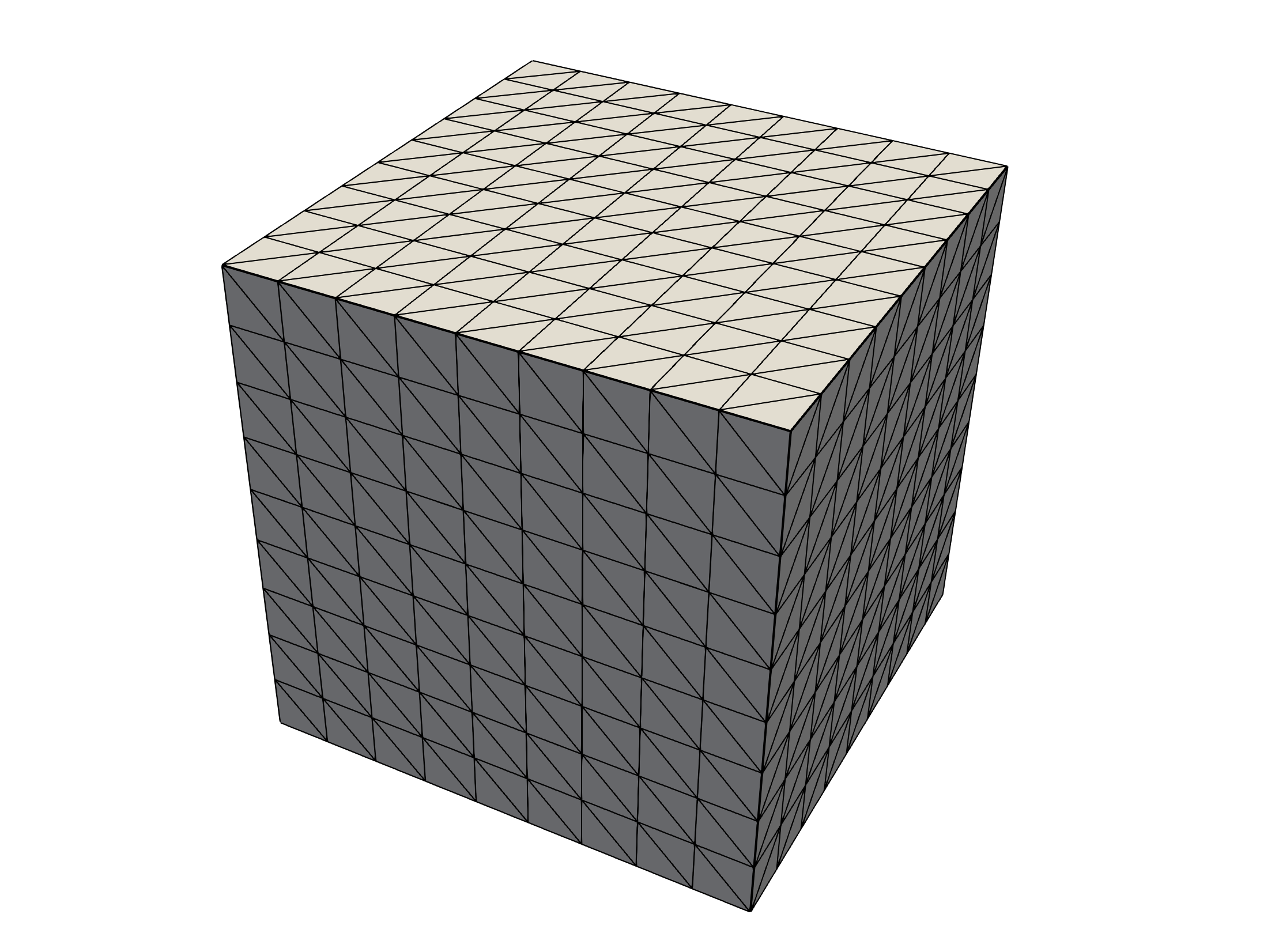
(a) Regular tetrahedral mesh with $4\,374$ cells

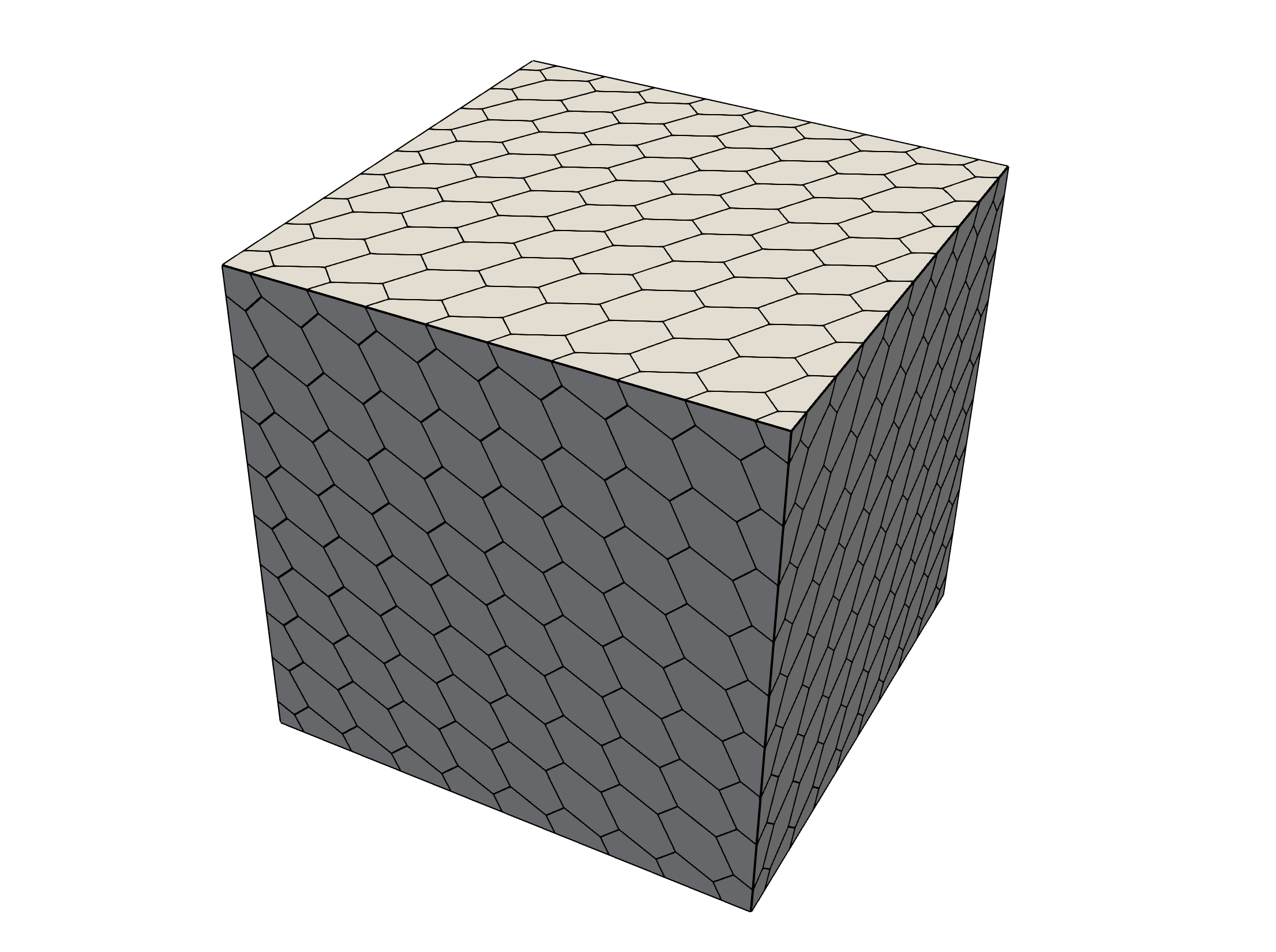
(b) Regular polyhedral mesh with $1\,000$ cells

(c) Regular hexahedral mesh with $1\,000$ cells

(d) Distorted hexahedral mesh with $1\,000$ cells

Figure 22: Meshes used in the method of manufactured solutions case

Appendix E Analytical Expressions for the Stress and Displacement Distributions around a Spherical Cavity under Uniaxial Tensions

The analytical expressions for the stress distributions around the cavity, first derived by Southwell and Gough [47], are

$$\sigma_{rr} = \frac{T}{14-10\nu}\frac{a^{3}}{R^{3}}\left[9-15\nu-12\frac{a^{2}}{R^{2}}-\frac{r^{2}}{R^{2}}\left(72-15\nu-105\frac{a^{2}}{R^{2}}\right)+15\frac{r^{4}}{R^{4}}\left(5-7\frac{a^{2}}{R^{2}}\right)\right],$$ (69)

$$\sigma_{\theta\theta} = \frac{T}{14-10\nu}\frac{a^{3}}{R^{3}}\left[9-15\nu-12\frac{a^{2}}{R^{2}}-15\frac{r^{2}}{R^{2}}\left(1-2\nu-\frac{a^{2}}{R^{2}}\right)\right],$$ (70)

$$\sigma_{zz} = T\left[1-\frac{1}{14-10\nu}\frac{a^{3}}{R^{3}}\left\{38-10\nu-24\frac{a^{2}}{R^{2}}-\frac{r^{2}}{R^{2}}\left(117-15\nu-120\frac{a^{2}}{R^{2}}\right)+15\frac{r^{4}}{R^{4}}\left(5-7\frac{a^{2}}{R^{2}}\right)\right\}\right],$$

$$\sigma_{zr} = \frac{T}{14-10\nu}\frac{a^{3}zr}{R^{5}}\left[-3(19-5\nu)+60\frac{a^{2}}{R^{2}}+15\frac{r^{2}}{R^{2}}\left(5-7\frac{a^{2}}{R^{2}}\right)\right].$$ (72)

where $a$ is the hole radius, $T$ is the distant stress applied in the $z$ direction, $\nu$ is the Poisson’s ratio, $r^{2}=x^{2}+y^{2}$ is the cylinderical radial coordinate, $R^{2}=r^{2}+z^{2}$ is the spherical radial coodinate, and $x$, $y$, $z$ are the Cartesian coordinates.

The displacement distributions were later derived by Goodier [48]:

$$u_{r} = -\frac{A}{r^{2}}-\frac{3B}{r^{4}}+\left[\frac{5-4\nu}{1-2\nu}\frac{C}{r^{2}}-9\frac{B}{r^{4}}\right]\cos(2\theta),$$ (73)

$$u_{\theta} = -\left[\frac{2C}{r^{2}}+6\frac{B}{r^{4}}\right]\sin(2\theta),$$ (74)

where the constants $A$, $B$ and $C$ are defined as follows:

$$\frac{A}{a^{3}}=-\frac{T}{8\mu}\frac{13-10\nu}{7-5\nu},\qquad\frac{B}{a^{5}}=-\frac{T}{8\mu}\frac{1}{7-5\nu},\qquad\frac{C}{a^{3}}=-\frac{T}{8\mu}\frac{5(1-2\nu)}{7-5\nu}.$$ (75)

and $\mu$ is the shear modulus.

References

- \bibcommenthead
- Trangenstein and Colella [1991] Trangenstein, J.A., Colella, P.: A higher-order Godunov method for modeling finite deformation in elastic-plastic solids. Communications on Pure and Applied Mathematics 44, 41–100 (1991)
- Kluth and Després [2010] Kluth, G., Després, B.: Discretization of hyperelasticity on unstructured mesh with a cell-centered Lagrangian scheme. Journal of Computational Physics 229, 9092–9118 (2010)
- Lee et al. [2013] Lee, C.H., Gil, A.J., Bonet, J.: Development of a cell centred upwind finite volume algorithm for a new conservation law formulation in structural dynamics. Computers & Structures 118, 13–38 (2013)
- Haider et al. [2017] Haider, J., Lee, C.H., Gil, A.J., Bonet, J.: A first order hyperbolic framework for large strain computational solid dynamics: An upwind cell centred total Lagrangian scheme. International Journal for Numerical Methods in Engineering 109, 407–456 (2017)
- Demirdžić et al. [1988] Demirdžić, I., Martinović, D., Ivanković, A.: Numerical simulation of thermal deformation in welded workpiece. Zavarivanje 31, 209–219 (1988). In Croatian. English translation available at https://www.researchgate.net/profile/Alojz_Ivankovic/publication/296148474_Numerical_simulation_of_thermal_deformation_in_welded_workpiece/links/5d07642ba6fdcc39f12219eb/Numerical-simulation-of-thermal-deformation-in-welded-workpiece.pdf
- Fryer et al. [1991] Fryer, Y.D., Bailey, C., Cross, M., Lai, C.-H.: A control volume procedure for solving the elastic stress-strain equations on an unstructured mesh. Applied Mathematical Modelling 15, 639–645 (1991)
- Demirdžić and Muzaferija [1995] Demirdžić, I., Muzaferija, S.: Numerical method for coupled fluid flow, heat transfer and stress analysis using unstructured moving meshes with cells of arbitrary topology. Computer Methods in Applied Mechanics and Engineering 125(1), 235–255 (1995) https://doi.org/10.1016/0045-7825(95)00800-G
- Jasak and Weller [2000] Jasak, H., Weller, H.G.: Application of the finite volume method and unstructured meshes to linear elasticity. International Journal for Numerical Methods in Engineering 48(2), 267–287 (2000) https://doi.org/10.1002/(SICI)1097-0207(20000520)48:2<267::AID-NME884>3.0.CO;2-Q https://onlinelibrary.wiley.com/doi/pdf/10.1002/%28SICI%291097-0207%2820000520%2948%3A2%3C267%3A%3AAID-NME884%3E3.0.CO%3B2-Q
- Tuković et al. [2013] Tuković, Ž., Ivanković, A., Karač, A.: Finite-volume stress analysis in multi-material linear elastic body. International Journal for Numerical Methods in Engineering 93(4), 400–419 (2013) https://doi.org/10.1002/nme.4390 https://onlinelibrary.wiley.com/doi/pdf/10.1002/nme.4390
- Cardiff et al. [2017] Cardiff, P., Tuković, Ž., Jaeger, P.D., Clancy, M., Ivanković, A.: A Lagrangian cell-centred finite volume method for metal forming simulation. International Journal for Numerical Methods in Engineering 109(13), 1777–1803 (2017) https://doi.org/10.1002/nme.5345 https://onlinelibrary.wiley.com/doi/pdf/10.1002/nme.5345
- Tuković et al. [2018] Tuković, Ž., Karač, A., Cardiff, P., Jasak, H., Ivanković, A.: OpenFOAM finite volume solver for fluid-solid interaction. Transactions of FAMENA 42(3), 1–31 (2018) https://doi.org/10.21278/TOF.42301
- Batistić et al. [2022] Batistić, I., Cardiff, P., Tuković, Ž.: A finite volume penalty based segment-to-segment method for frictional contact problems. Applied Mathematical Modelling 101, 673–693 (2022) https://doi.org/10.1016/j.apm.2021.09.009
- Das et al. [2011] Das, S., Mathur, S.R., Murthy, J.Y.: An Unstructured Finite-Volume Method for Structure–Electrostatics Interactions in MEMS. Numerical Heat Transfer, Part B: Fundamentals 60(6), 425–451 (2011) https://doi.org/10.1080/10407790.2011.628252 https://doi.org/10.1080/10407790.2011.628252
- Cardiff et al. [2016] Cardiff, P., Tuković, Ž., Jasak, H., Ivanković, A.: A block-coupled finite volume methodology for linear elasticity and unstructured meshes. Computers & Structures 175, 100–122 (2016) https://doi.org/10.1016/j.compstruc.2016.07.004
- Castrillo et al. [2024] Castrillo, P., Schillaci, E., Rigola, J.: High-order cell-centered finite volume method for solid dynamics on unstructured meshes. Computers & Structures 295, 107288 (2024) https://doi.org/10.1016/j.compstruc.2024.107288
- McHugh and Knoll [1994] McHugh, P.R., Knoll, D.A.: Comparison of standard and matrix-free implementations of several Newton–Krylov solvers. AIAA Journal 32(12), 2394–2400 (1994) https://doi.org/10.2514/3.12305
- Qin et al. [2000] Qin, N., Ludlow, D.K., Shaw, S.T.: A matrix-free preconditioned Newton/GMRES method for unsteady Navier–Stokes solutions. International Journal for Numerical Methods in Fluids 33(2), 223–248 (2000) https://doi.org/10.1002/(SICI)1097-0363(20000530)33:2<223::AID-FLD10>3.0.CO;2-V
- Geuzaine [2001] Geuzaine, P.: Newton-Krylov strategy for compressible turbulent flows on unstructured meshes. AIAA Journal 39(3), 528–531 (2001) https://doi.org/10.2514/2.1339
- Pernice and Tocci [2001] Pernice, M., Tocci, M.D.: A multigrid-preconditioned Newton–Krylov method for the incompressible Navier–Stokes equations. SIAM Journal on Scientific Computing 23(2), 398–418 (2001) https://doi.org/10.1137/S1064827500372250
- Knoll and Keyes [2004] Knoll, D.A., Keyes, D.E.: Jacobian-free Newton–Krylov methods: a survey of approaches and applications. Journal of Computational Physics 193(2), 357–397 (2004) https://doi.org/10.1016/j.jcp.2003.08.010
- Nejat and Ollivier-Gooch [2008] Nejat, A., Ollivier-Gooch, C.: A high-order accurate unstructured finite volume Newton–Krylov algorithm for inviscid compressible flows. Journal of Computational Physics 227(4), 2582–2609 (2008) https://doi.org/10.1016/j.jcp.2007.11.011
- Vaassen et al. [2008] Vaassen, J.-M., Vigneron, D., Essers, J.-A.: An implicit high order finite volume scheme for the solution of 3d Navier–Stokes equations with new discretization of diffusive terms. Journal of Computational and Applied Mathematics 215(2), 595–601 (2008) https://doi.org/10.1016/j.cam.2006.04.066
- Lucas et al. [2010] Lucas, P., Zuijlen, A.H., Bijl, H.: Fast unsteady flow computations with a jacobian-free Newton–Krylov algorithm. Journal of Computational Physics 229(24), 9201–9215 (2010) https://doi.org/10.1016/j.jcp.2010.08.033
- Nejat et al. [2011] Nejat, A., Jalali, A., Sharbatdar, M.: A Newton–Krylov finite volume algorithm for the power-law non-Newtonian fluid flow using pseudo-compressibility technique. Journal of Non-Newtonian Fluid Mechanics 166(19–20), 1158–1172 (2011) https://doi.org/10.1016/j.jnnfm.2011.07.003
- Nishikawa [2020] Nishikawa, H.: A hyperbolic poisson solver for tetrahedral grids. Journal of Computational Physics 409, 109358 (2020) https://doi.org/10.1016/j.jcp.2020.109358
- Gear and Saad [1983] Gear, C.W., Saad, Y.: Iterative solution of linear equations in ODE codes. SIAM Journal on Scientific and Statistical Computing 4(4), 583–601 (1983) https://doi.org/10.1137/0904040
- Chan and Jackson [1984] Chan, T.F., Jackson, K.R.: Nonlinearly preconditioned Krylov subspace methods for discrete Newton algorithms. SIAM Journal on Scientific and Statistical Computing 5(3), 533–542 (1984) https://doi.org/10.1137/0905039
- Brown and Hindmarsh [1986] Brown, P.N., Hindmarsh, A.C.: Matrix-free methods for stiff systems of ODE’s. SIAM Journal on Numerical Analysis 23(3), 610–638 (1986) https://doi.org/10.1137/0723034
- Brown and Saad [1990] Brown, P.N., Saad, Y.: Hybrid Krylov methods for nonlinear systems of equations. SIAM Journal on Scientific and Statistical Computing 11(3), 450–481 (1990) https://doi.org/10.1137/0911026
- Badcock and Gaitonde [1996] Badcock, K.J., Gaitonde, A.L.: An unfactored implicit moving mesh method for the two-dimensional unsteady N-S equations. International Journal for Numerical Methods in Fluids 23(6), 607–631 (1996) https://doi.org/10.1002/(SICI)1097-0363(19960930)23:6<607::AID-FLD433>3.0.CO;2-E . First published: 30 September 1996
- Balay et al. [2015] Balay, S., Abhyankar, S., Adams, M.F., Brown, J., Brune, P., Buschelman, K., Dalcin, L., Eijkhout, V., Gropp, W.D., Kaushik, D., Knepley, M.G., McInnes, L.C., Rupp, K., Smith, B.F., Zampini, S., Zhang, H.: PETSc Web page. http://www.mcs.anl.gov/petsc (2015). http://www.mcs.anl.gov/petsc
- Nishikawa et al. [2017] Nishikawa, H., Nakashima, Y., Watanabe, N.: Effects of high-frequency damping on iterative convergence of implicit viscous solver. Journal of Computational Physics 348, 66–81 (2017) https://doi.org/10.1016/j.jcp.2017.07.021
- Weller et al. [1998] Weller, H.G., Tabor, G., Jasak, H., Fureby, C.: A tensorial approach to computational continuum mechanics using object orientated techniques. Computers in Physics 12, 620–631 (1998)
- Jasak [1996] Jasak, H.: Error analysis and estimation for the finite volume method with applications to fluid flows. PhD thesis, Imperial College London (University of London) (1996)
- Demirdžić and Cardiff [2022] Demirdžić, I., Cardiff, P.: Symmetry plane boundary conditions for cell-centered finite-volume continuum mechanics. Numerical Heat Transfer, Part B: Fundamentals (2022) https://doi.org/10.1080/10407790.2022.2105073
- Jasak [2011] Jasak, H.: Finite Volume Discretisation with Polyhedral Cell Support: What is Discretisation? Presentation at NUMAP-FOAM Summer School, Zagreb, Croatia, 2-15 September 2009 (2011). https://www.slideshare.net/slideshow/57969246-finitevolume/16128767
- Syrakos et al. [2023] Syrakos, A., Oxtoby, O., Villiers, E., Varchanis, S., Dimakopoulos, Y., Tsamopoulos, J.: A unification of least-squares and green–gauss gradients under a common projection-based gradient reconstruction framework. Mathematics and Computers in Simulation 205, 108–141 (2023) https://doi.org/10.1016/j.matcom.2022.09.008
- Rhie and Chow [1983] Rhie, C.M., Chow, W.L.: Numerical study of the turbulent flow past an airfoil with trailing edge separation. AIAA Journal 21(11), 1525–1532 (1983) https://doi.org/10.2514/3.8284 https://doi.org/10.2514/3.8284
- Cardiff et al. [2018] Cardiff, P., Karač, A., Jaeger, P.D., Jasak, H., Nagy, J., Ivanković, A., Tuković, Ž.: An open-source finite volume toolbox for solid mechanics and fluid-solid interaction simulations (2018) https://doi.org/10.48550/arXiv.1808.10736 . https://arxiv.org/abs/1808.10736
- Nishikawa [2010] Nishikawa, H.: Beyond interface gradient: A general principle for constructing diffusion schemes. In: 40th Fluid Dynamics Conference and Exhibit. AIAA, Chicago, Illinois, USA (2010). https://doi.org/10.2514/6.2010-5093 . Published online: 13 Nov 2012
- Jsvobs [1986] Jsvobs, D.A.H.: A Generalization of the Conjugate-Gradient Method to Solve Complex Systems. IMA Journal of Numerical Analysis 6(4), 447–452 (1986) https://doi.org/10.1093/imanum/6.4.447 https://academic.oup.com/imajna/article-pdf/6/4/447/2181350/6-4-447.pdf
- Falgout and Yang [2002] Falgout, R.D., Yang, U.M.: hypre: A library of high performance preconditioners. In: Sloot, P.M.A., Hoekstra, A.G., Tan, C.J.K., Dongarra, J.J. (eds.) Computational Science — ICCS 2002, pp. 632–641. Springer, Berlin, Heidelberg (2002)
- Amestoy et al. [2001] Amestoy, P.R., Duff, I.S., Koster, J., L’Excellent, J.-Y.: A fully asynchronous multifrontal solver using distributed dynamic scheduling. SIAM Journal on Matrix Analysis and Applications 23(1), 15–41 (2001)
- Amestoy et al. [2019] Amestoy, P.R., Buttari, A., L’Excellent, J.-Y., Mary, T.: Performance and Scalability of the Block Low-Rank Multifrontal Factorization on Multicore Architectures. ACM Transactions on Mathematical Software 45, 2–1226 (2019)
- Mazzanti [2024] Mazzanti, F.: Coupled vertex-centred finite volume methods for large-strain elastoplasticity. PhD thesis, University College Dublin (2024). For examination
- Geuzaine and Remacle [2009] Geuzaine, C., Remacle, J.-F.: Gmsh: A 3-d finite element mesh generator with built-in pre- and post-processing facilities. International journal for numerical methods in engineering 79(11), 1309–1331 (2009) https://doi.org/10.1002/nme.2579
- Southwell and Gough [1926] Southwell, R.V., Gough, H.J.: Vi. on the concentration of stress in the neighbourhood of a small spherical flaw; and on the propagation of fatigue fractures in “statistically isotropic” materials. The London, Edinburgh, and Dublin Philosophical Magazine and Journal of Science 1(1), 71–97 (1926) https://doi.org/10.1080/14786442608633614 https://doi.org/10.1080/14786442608633614
- Goodier [1933] Goodier, J.N.: Concentration of stress around spherical and cylindrical inclusions and flaws. Journal of Applied Mechanics 1(2), 39–44 (1933)
- Hitchings et al. [1987] Hitchings, D., Davies, G.A.O., Kamoulakos, A.: Linear Static Benchmarks. International Association for the Engineering Analysis Community & National Agency for Finite Element Methods & Standards (NAFEMS), Glasgow, UK (1987)
- Demirdžić et al. [1997] Demirdžić, I., Muzaferija, S., Perić, M.: Advances in computation of heat transfer, fluid flow, and solid body deformation using finite volume approaches. In: W. J. Minkowycz, E.M.S. (ed.) Advances in Numerical Heat Transfer, Chapter 2, pp. 59–96. Taylor & Francis, London, United Kingdom (1997)
- Cardiff et al. [2016] Cardiff, P., Tuković, Jasak, H., Ivanković, A.: A block-coupled finite volume methodology for linear elasticity and unstructured meshes. Computers & Structures 175, 100–122 (2016) https://doi.org/10.1016/j.compstruc.2016.07.004
- [52] Rohatgi, A.: WebPlotDigitizer. https://automeris.io
- Land et al. [2015] Land, S., Gurev, V., Arens, S., Augustin, C.M., Baron, L., Blake, R., Bradley, C., Castro, S., Crozier, A., Favino, M., Fastl, T.E., Fritz, T., Gao, H., Gizzi, A., Griffith, B.E., Hurtado, D.E., Krause, R., Luo, X., Nash, M.P., Pezzuto, S., Plank, G., Rossi, S., Ruprecht, D., Seemann, G., Smith, N.P., Sundnes, J., Rice, J.J., Trayanova, N., Wang, D., Wang, Z.J., Niederer, S.A.: Verification of cardiac mechanics software: benchmark problems and solutions for testing active and passive material behaviour 471(2184), 20150641 (2015) https://doi.org/10.1098/rspa.2015.0641
- Guccione et al. [1995] Guccione, J.M., Costa, K.D., McCulloch, A.D.: Finite element stress analysis of left ventricular mechanics in the beating dog heart. Journal of Biomechanics 28(10), 1167–1177 (1995) https://doi.org/10.1016/0021-9290(94)00174-3
- Zienkiewicz and Taylor [2000] Zienkiewicz, O.C., Taylor, R.L.: The Finite Element Method vol. 2. Butterworth-heinemann, Berlin, Germany (2000)
- [56] Areias, P.: Simplas. Portuguese Software Association (ASSOFT). http://www.simplassoftware.com.
- Pelteret and McBride [2018] Pelteret, J.-P., McBride, A.: The deal.II code gallery: Quasi-Static Finite-Strain Compressible Elasticity. Zenodo (2018). https://doi.org/10.5281/zenodo.1228964 . https://doi.org/10.5281/zenodo.1228964
- Simo and Armero [1992] Simo, J.C., Armero, F.: Geometrically non-linear enhanced strain mixed methods and the method of incompatible modes. International Journal for Numerical Methods in Engineering 33(7), 1413–1449 (1992) https://doi.org/10.1002/nme.1620330705 https://onlinelibrary.wiley.com/doi/pdf/10.1002/nme.1620330705
- César de Sá et al. [2001] Sá, J.M.A., Areias, P.M.A., Natal Jorge, R.M.: Quadrilateral elements for the solution of elasto-plastic finite strain problems. International Journal for Numerical Methods in Engineering 51(8), 883–917 (2001) https://doi.org/10.1002/nme.183 https://onlinelibrary.wiley.com/doi/pdf/10.1002/nme.183
- Tuković and Jasak [2007] Tuković, Ž., Jasak, H.: Updated Lagrangian finite volume solver for large deformation dynamic response of elastic body. Transactions of FAMENA 31(1), 55–70 (2007)
- Turek and Hron [2006] Turek, S., Hron, J.: Proposal for numerical benchmarking of fluid-structure interaction between an elastic object and laminar incompressible flow. In: Bungartz, H.-J., Schäfer, M. (eds.) Fluid-Structure Interaction: Modelling, Simulation, Optimisation. Lecture Notes in Computational Science and Engineering, vol. 53, pp. 371–385. Springer, Berlin, Heidelberg (2006). https://doi.org/10.1007/3-540-34596-5_20
- Ferziger and Peric [2002] Ferziger, J.H., Peric, M.: Computational Methods for Fluid Dynamics, 3rd edn. Springer, Berlin, Germany (2002)
- Degroote et al. [2009] Degroote, J., Bathe, K.-J., Vierendeels, J.: Performance of a new partitioned procedure versus a monolithic procedure in fluid-structure interaction. Computers & Structures 87(11-12), 793–801 (2009) https://doi.org/10.1016/j.compstruc.2009.01.006
- Pellegrini [2012] Pellegrini, F.: Scotch and PT-Scotch graph partitioning software: An overview. In: Naumann, U., Schenk, O. (eds.) Combinatorial Scientific Computing, pp. 373–406. Chapman and Hall/CRC, London, United Kingdom (2012). Chap. 14. https://doi.org/10.1201/b11644-15 . https://hal.inria.fr/hal-00770422
- Simo and Hughes [1998] Simo, J.C., Hughes, T.J.R.: Computational Inelasticity vol. 7. Springer, New York (1998)