Peakons and pseudo-peakons of higher order b-family equations

Abstract

The peakon equations have garnered significant attention due to their rich mathematical structure and potential applications in various physical contexts. In this study, we extend the well-known b-family system, $m_{t}+m_{x}v+bv_{x}m=0,\quad m=(1-\partial_{x}^{2})v,$ to a more general higher-order one with $m=(1-\partial_{x}^{2})^{J}v$ for an arbitrary positive integer $J$. We conjecture the existence of a b-independent pseudo-peakon solution of the form, $v=c\left(1+\left|x-ct\right|+\sum_{i=1}^{J-2}a_{i}\left|x-ct\right|^{i+1}\right)\mbox{\rm e}^{-\left|x-ct\right|}$ which includes $J-1$ arbitrary constants $a_{1},\ a_{2},\ \cdots,\ a_{J-1}$ for all $J\geq 2$. In additional to the b-independent psudo-peakon solution, we conclude that there are one b-independent peakon, one b-dependent peakon (for odd J) or two b-dependent peakons (for even J), and $J-3$ (for odd J) or $J-4$ (for even J) complex peakons. This comprehensive analysis provides deeper insights into the structure and behavior of peakons and pseudo-peakons within the extended b-family framework.

The b-family of equations represents a significant class of nonlinear partial differential equations that have garnered substantial attention in the field of mathematical physics. These equations are known for their rich structure and the presence of peakon solutions, which are solitary waves with a peak at their crest. The general form of the b-family equation is given by:

$$m_{t}+vm_{x}+bv_{x}m=0,\quad m=(1-\partial_{x})^{2}v,$$ (1)

where $b$ is a parameter that influences the nonlinearity and dispersion properties of the equation.

The study of the b-family equations has provided significant insights into nonlinear wave behavior, particularly through the discovery of peakon solutions-weak solutions with discontinuous first derivatives at their peaks. These solutions have been widely studied due to their unique properties and physical applications.

Camassa and Holm CH introduced the Camassa-Holm equation, a special case of the b-family with $b=2$, which admits peakon solutions. This foundational work spurred further research into the integrability and stability of peakons. Degasperis and Procesi DP derived another member of the b-family for $b=3$, the Degasperis-Procesi equation, which also supports peakons and exhibits a bi-Hamiltonian structure, emphasizing its integrability.

The concept of pseudo-peakons, smooth approximations of peakons, has further enriched the field. Research by Lenells Lenells and others has explored their properties and stability, bridging the gap between smooth solitons and peakons. Constantin and Strauss CS investigated peakon stability, while Ivanov Ivanov advanced the understanding of higher-order b-family equations. Holm and Staley HS analyzed wave structures and nonlinear balances in evolutionary PDEs, contributing to the dynamics of peakon systems. Johnson Johnson connected the Camassa-Holm and Korteweg-de Vries equations, enhancing their relevance in water wave modeling. Olver-Rosenau OR and Chen-Liu-Zhang CLZ generalized the Camassa-Holm equation to two components, expanding solution scopes and integrability insights.

Recent advancements have extended the b-family and related models to higher-order formulations HIS ; Lou ; Fokas . Henry, Ivanov, and Sakellaris HIS extended the CH and DP equations, offering a theoretical framework for oceanic internal wave-current interactions. Gorka, Pons, and Reyes GPR explored higher-order Camassa-Holm equations using loop group geometry, while Liu and Qiao LiuQiao introduced pseudo-peakons and multi-peakons in a fifth-order model. Qiao and Reyes QR further advanced the field with fifth-order extensions, broadening the understanding of nonlinear wave phenomena.

In this letter, we investigate the peakon and pseudo-peakon structures for a class of higher-order b-family equations, defined as

$$m_{t}+vm_{x}+bv_{x}m=0,\quad m=(1-\partial_{x}^{2})^{J}v,$$ (2)

where $J$ is an arbitrary positive integer. For notational convenience, we refer to (2) as the $J$-th b-family ($J$-bF) equation. Specifically, when $b=2$, the equation is termed the $J$-th Camassa-Holm ($J$-CH) equation, and for $b=3$, it is referred to as the $J$-th Degasperis-Procesi ($J$-DP) equation. The loop group geometric aspects of the $J$-CH equation have been previously explored in GPR .

Through extensive and intricate calculations on the weak solutions of the $J$-bF system (2) for various values of $J$, we propose the following conjecture:
Conjecture. The $J$-bF equation (2) admits a $b$-independent pseudo-peakon solution

$$v=c\left(1+|x-ct|+\sum_{i=1}^{J-2}a_{i}|x-ct|^{i+1}\right)\mbox{\rm e}^{-|x-ct|},\quad\forall J\geq 2,$$ (3)

where $a_{1},a_{2},\dots,a_{J-2}$ are arbitrary constants.

The conjecture has been verified for the cases of $J\leq 14$ by means of the computer algebra MAPLE. While a clear path to a general proof remains elusive at this stage, we are hopeful that a proof will be established by researchers in the near future.

The simplest scenario, corresponding to $J=2$ in equation (3), has been previously established by several researchers. However, the generalized solution (3) for any $J>2$ is introduced for the first time in this paper. The pseudo-peakon solution (3) exhibits a rich and intricate structure. In this letter, we explore specific instances for various values of $J$. Prior to delving into particular cases, we provide a formal definition of the $n$th pseudo-peakon.
Definition. A solution is termed the $n$th pseudo-peakon if its $i$th-order $x$-derivatives are continuous for all $i\leq n-1$, while the $n$th-order $x$-derivative is discontinuous.
Case 1. $J=2$, 3rd pseudo-peakon. In this particular case, the model (2) becomes ($v_{xi}=v_{x^{i}}$)

$$m_{t}+vm_{x}+bv_{x}m=0,\quad m=v-2v_{xx}+v_{x4},$$ (4)

while the solution (3) is given by

$$v=v_{J=2}=c(1+|x-ct|)\mbox{\rm e}^{-|x-ct|},$$ (5)

which shares the same functional form as a solution to another fifth-order CH equation QR . The solution (5) is classified as a 3rd pseudo-peakon but not a peakon (1st pseudo-peakon). This distinction arises because the first and second order derivatives of $u$ are continuous, satisfying $v_{x}(x=c(t+0^{+}))=v_{x}(x=c(t+0^{-}))\quad\text{and}\quad v_{xx}(x=c(t+0^{+}))=v_{xx}(x=c(t+0^{-})),$ while the third order derivative is discontinuous, i.e., $v_{x3}(x=c(t+0^{+}))\neq v_{x3}(x=c(t+0^{-})).$

In addition to the 3rd pseudo-peakon solution (5), we can find a previously unknown $b$-independent peakon solution

$$v=\frac{1}{2}c\left(2+|x-ct|\right)\mbox{\rm e}^{-|x-ct|},$$ (6)

for the $2$-bF equation (4).
Case 2. $J=3$, 3rd and 5th pseudo-peakons. For $J=3$, the model (2) and the solution (3) are given by

$$m_{t}+vm_{x}+bv_{x}m=0,\quad m=v-3v_{xx}+3v_{x4}-v_{x6},$$ (7)

$$v=v_{J=3}=c\left(1+|x-ct|+a_{1}|x-ct|^{2}\right)\mbox{\rm e}^{-|x-ct|}.$$ (8)

The solution (8) represents a 3rd pseudo-peakon for a general constant $a_{1}\neq\frac{1}{3}$, while it reduces to a 5th pseudo-peakon for the specific constant $a_{1}=\frac{1}{3}$. Figs. 1(a)–1(d) illustrate the intricate structure of the pseudo-peakon (8) for parameter choices $a=-2$, $-50$, $2$, and $\frac{1}{2}$, respectively, at time $t=0$. The velocity parameter $c$ and the time $t$ are fixed at $c=1$ and $t=0$ for all figures in this paper. Fig. 1(e) demonstrates the structure of the second-order partial derivative, $v_{xx}$, at the center of the pseudo-peakon (8) with $a=\frac{1}{2}$. Similarly, Fig. 1(f) highlights the property of the fourth-order partial derivative, $v_{x4}$, at the center of the pseudo-peakon (8) with $a=\frac{1}{3}$. The Figures 1(e) and 1(f) indicate also the discontinuous of the third and the fifth order partial derivatives of the field $v$ with respect to $x$.

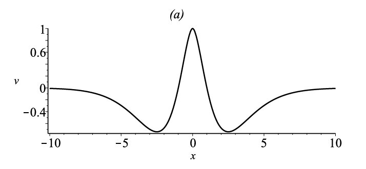
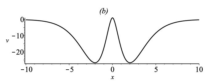
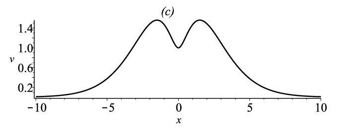
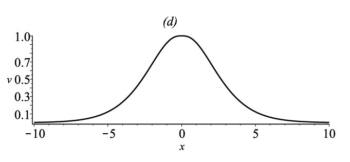
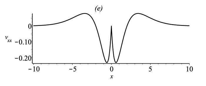
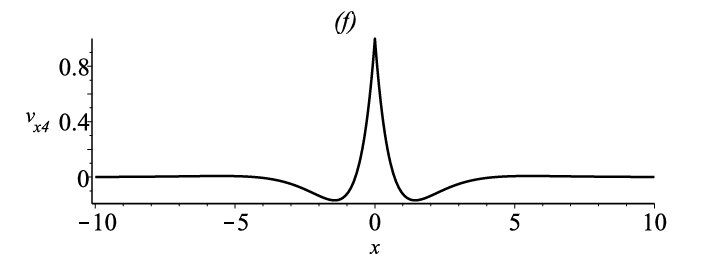
Figure 1: (a) Pseudo-peakon structure with one smooth peak and double bottoms expressed by (8) and $a=-2$; (b) W-shaped pseudo-peakon structure given by (8) and $a=-50$; (c) M-shaped pseudo-peakon structure of (8) with $a=2$; (d) Pseudo-peakon structure with a single smooth peak expressed by (8) and $a=\frac{1}{2}$; (e) The structure of the second-order derivative of the 3rd pseudo-peakon (8) with $a=\frac{1}{2}$; (f) The structure of the fourth-order derivative of the 5th pseudo-peakon (8) with $a=\frac{1}{3}$.

Similar to the case of $J=2$, the $3$-bF model (7) also admits a $b$-independent peakon solution of the form

$$v=\frac{1}{138}c\left(138+72|x-ct|+13|x-ct|^{2}\right)\mathrm{e}^{-|x-ct|}.$$ (9)

The structure of this $b$-independent peakon (9) is illustrated in Fig. 2(a) for the amplitude $c=1$ at time $t=0$.

In contrast to the $J=2$ case, there exists a $b$-dependent peakon solution given by

$$v=\frac{653c}{385923-67196b}\left(591+289|x-ct|+46|x-ct|^{2}\right)\mathrm{e}^{-|x-ct|}.$$ (10)

Fig. 2(b) depicts the structure of this $b$-dependent peakon (10) with the amplitude $\frac{385923c}{385923-67196b}$ at time $t=0$. For this solution, a critical value of $b$ exists, defined as $b_{\text{cr}}=\frac{385923c}{67196}\approx 5.743329c$. When the parameter $b$ transitions from $b>b_{\text{cr}}$ (with $c>0$) to $b<b_{\text{cr}}$, the peakon transforms into an anti-peakon. Moreover, as $b$ approaches the critical value $b_{\text{cr}}$, the amplitude of the peakon diverges to infinity.

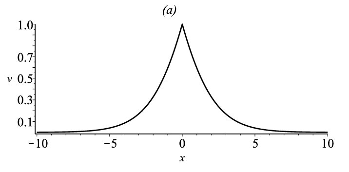
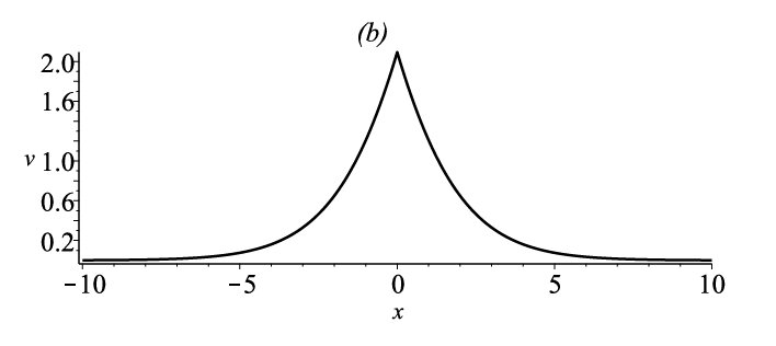
Figure 2: (a) The structure of the $b$-independent peakon expressed by (9); (b) The structure of the $b$-dependent peakon of (10) with $b=3$.

Case 3. $J=4$, $3$rd, $5$th, and $7$th pseudo-peakons. For $J=4$, the $J$-bF system (2) and the pseudo-peakon solution (3) take the form

$$m_{t}+vm_{x}+bv_{x}m=0,\quad m=v-4v_{xx}+6v_{x4}-4v_{x6}+v_{x8},$$ (11)

$$v=v_{J=4}=c\left(1+|x-ct|+a_{1}|x-ct|^{2}+a_{2}|x-ct|^{3}\right)\mathrm{e}^{-|x-ct|}.$$ (12)

The solution (12) corresponds to a 3rd-order pseudo-peakon for general constants $\{a_{1},a_{2},b,c\}$ under the condition $3(a_{2}-a_{1})+1\neq 0$. When $3(a_{2}-a_{1})+1=0$ but $a_{1}\neq\frac{2}{5}$, the solution (12) reduces to a 5th-order pseudo-peakon. Additionally, for the specific parameter values $\{a_{1}=\frac{2}{5},a_{2}=\frac{1}{15}\}$, (12) describes a 7th-order pseudo-peakon.

Figures 3(a)–3(d) illustrate the structure of the pseudo-peakon defined by (12) for the parameter sets $\{a_{1}=\frac{1}{2},a_{2}=\frac{1}{6}\}$, $\{a_{1}=1,a_{2}=1\}$, $\{a_{1}=-\frac{5}{4},a_{2}=1\}$, and $\{a_{1}=1,a_{2}=-30\}$, respectively. To demonstrate the discontinuous nature of the pseudo-peakon (12), Figures 3(e)–3(f) showcase the peak characteristics of the fourth and sixth derivatives of the field $v$ with respect to $x$.

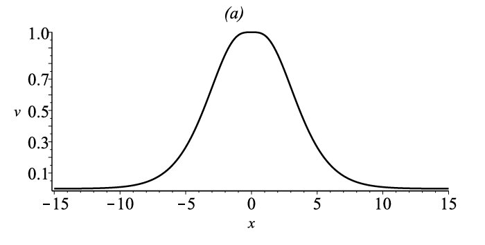
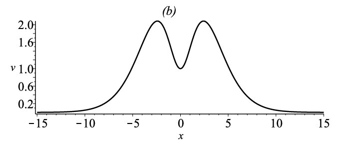
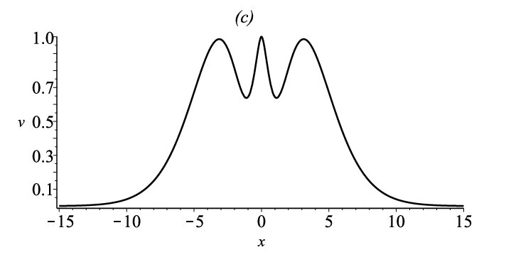
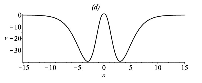
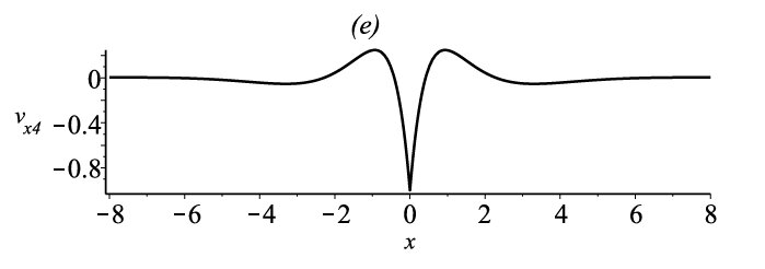
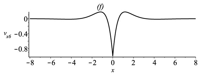
Figure 3: (a) A quite smooth pseudo-peakon (12) with $\{a_{1}=\frac{1}{2},\ a_{2}=\frac{1}{6}\}$ and $v_{x}|_{x=ct}=v_{xx}|_{x=ct}=v_{xxx}|_{x=ct}=0$; (b) M-shaped pseudo-peakon (12) with $a_{1}=a_{2}=1$; (c) The structure of the pseudo-peakon with three smooth peaks expressed by (12), $a_{1}=-\frac{5}{4}$ and $a_{2}=1$; (d) W-shaped pseudo-peakon (12) with $\{a_{1}=1,\ a_{2}=-30\}$; (e) The structure of the fourth-order derivative of $v$ with respect to $x$ for the 5th pseudo-peakon expressed by (12) with the same parameters as (a); (f) The structure of the sixth-order derivative of $v$ with respect to $x$ for the 7th pseudo-peakon given by (12) with the selections $\{a_{1}=\frac{2}{5},\ a_{2}=\frac{1}{15}\}$.

Similar to the case of $J=3$, the $3$-bF system admits not only the pseudo-peakon solution (12) but also several types of peakon solutions. The first peakon solution is independent of the parameter $b$ and takes the form

$$v=\frac{c}{3408}\left(3408+1485|x-ct|+243|x-ct|^{2}+16|x-ct|^{3}\right)\mathrm{e}^{-|x-ct|}.$$ (13)

In addition, there exist two $b$-dependent peakon solutions, which can be expressed in a unified form (with $\alpha\equiv 11461919(a_{0}-1)$):

$$v =\frac{c}{104709174912b}\left[24a_{0}b\left(21135531|x-ct|^{3}+312776708|x-ct|^{2}+1902237510|x-ct|\right.\right.$$

$$\quad\left.\left.+4362882288\right)+\alpha\left(343|x-ct|^{3}+2272|x-ct|^{2}+4758|x-ct|\right)\right]\mathrm{e}^{-|x-ct|},$$ (14)

where the parameter $a_{0}$ takes on two distinct values:

$$a_{0}=\frac{1}{27905650366969405}\left(23586956522630821\pm 288\sqrt{56775579142818640974199474}\right).$$ (15)

The structures of the solutions (13) and (14) are qualitatively similar to those illustrated in Figures 2(a)–2(b).
Case 4. $J=5$, 3rd, 5th, 7th, and 9th pseudo-peakons. For $J=5$, the $J$-bF system (2) and the pseudo-peakon solution (3) take the form

$$m_{t}+vm_{x}+bv_{x}m=0,\quad m=v-5v_{xx}+10v_{x4}-10v_{x6}+5v_{x8}-v_{x10},$$ (16)

$$v=v_{J=5}=c\left(1+|x-ct|+a_{1}|x-ct|^{2}+a_{2}|x-ct|^{3}+a_{3}|x-ct|^{4}\right)\mathrm{e}^{-|x-ct|}.$$ (17)

The solution (17) represents a $b$-independent 3rd pseudo-peakon for arbitrary constants $\{a_{1},a_{2},a_{3},b,c\}$, provided that $3(a_{2}-a_{1})+1\neq 0$. When $3(a_{2}-a_{1})+1=0$ but $5(3a_{3}-a_{1})+2c\neq 0$, the solution (17) simplifies to a 5th pseudo-peakon. For $\{3(a_{2}-a_{1})+1=0,5(3a_{3}-a_{1})+2c=0\}$ but with $7a_{1}\neq 3c$, the solution (17) corresponds to a 7th pseudo-peakon. Finally, for the specific parameter values $\{a_{1}=\frac{3}{7},a_{2}=\frac{2}{21},a_{3}=\frac{1}{105}\}$, (17) describes a 9th pseudo-peakon.

Figures 4(a)–4(f) illustrate the $b$-independent pseudo-peakon (17) with the following parameter selections: $\{a_{1}=10,a_{2}=-7,a_{3}=1\}$, $\{a_{1}=1,a_{2}=-5,a_{3}=1\}$, $\{a_{1}=1,a_{2}=1,a_{3}=1\}$, $\{a_{1}=\frac{1}{2},a_{2}=\frac{1}{5},a_{3}=\frac{1}{10}\}$, $\{a_{1}=\frac{3}{7},a_{2}=\frac{2}{21},a_{3}=\frac{1}{105}\}$, and $\{a_{1}=\frac{1}{2},a_{2}=\frac{1}{5},a_{3}=-2\}$, respectively. Meanwhile, Figs. 4(g)–4(h) demonstrate that the 9th pseudo-peakon solution (17) with $\{a_{1}=\frac{3}{7},a_{2}=\frac{2}{21},a_{3}=\frac{1}{105}\}$ exhibits continuous derivatives of $v$ up to the eighth order.

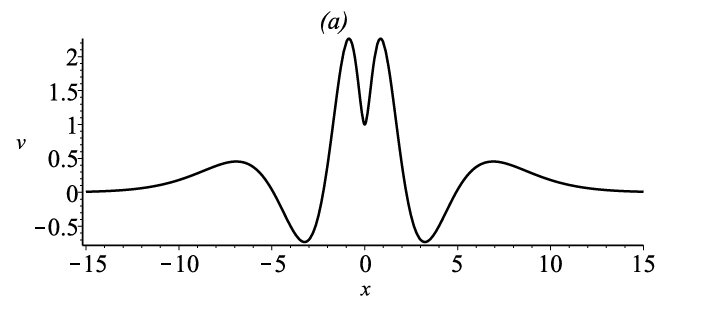
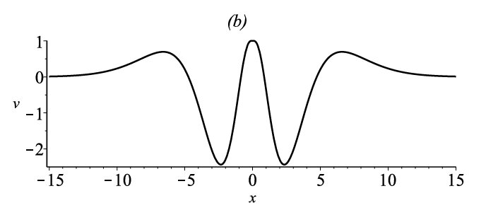
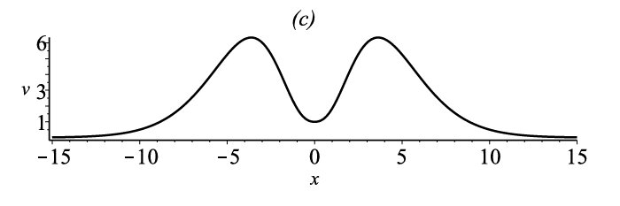
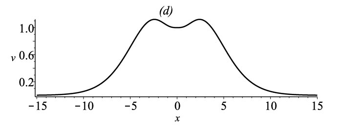
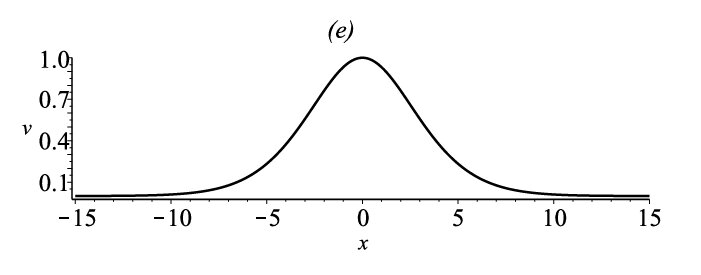
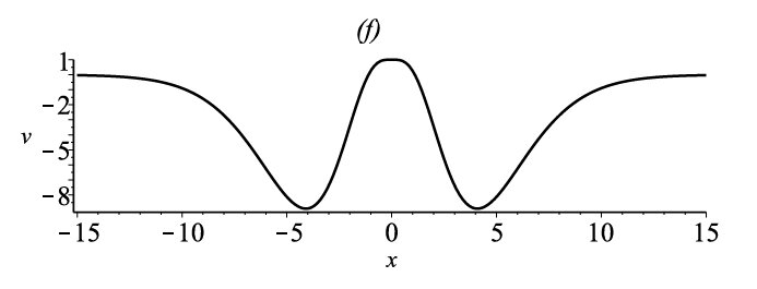
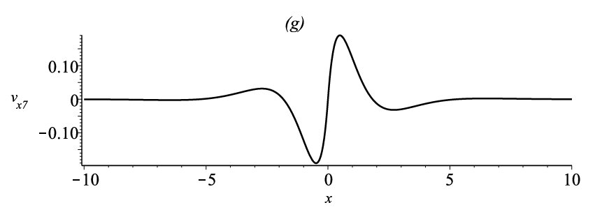
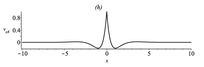
Figure 4: (a) Pseudo-peakon with four smooth peaks expressed by (17) and $\{a_{1}=10,\ a_{2}=-7,\ a_{3}=1\}$; (b) Pseudo-peakon with three smooth peaks given by (17) and $\{a_{1}=1,\ a_{2}=-5,\ a_{3}=1\}$; (c) M-shaped pseudo-peakon expressed by (17) with $\{a_{1}=10,\ a_{2}=1,\ a_{3}=1\}$; (d) Pseudo-peakon with double smooth peaks expressed by (17) and $\{a_{1}=\frac{1}{2},\ a_{2}=\frac{1}{5},\ a_{3}=\frac{1}{10}\}$; (e) Single smooth peaked pseudo-peakon expressed by (17) with $\{a_{1}=\frac{3}{7},\ a_{2}=\frac{2}{21},\ a_{3}=\frac{1}{105}\}$; (f) W-shaped pseudo-peakon expressed by (17) with $\{a_{1}=\frac{1}{2},\ a_{2}=\frac{1}{5},\ a_{3}=-2\}$; (g) The seventh-order derivative of $v$ with respect to $x$ of (e); (h) The eighth-order derivative of $v$ with respect to $x$ of (e).

The $b$-independent peakon solution of (16) is given by

$$v = \frac{c}{3493276440}\left(4120035|x-ct|^{4}+65760592|x-ct|^{3}+490916844|x-ct|^{2}\right.$$ (18)

$$\left.+1972076400|x-ct|+3493276440\right)\mathrm{e}^{-|x-ct|}.$$

For the $b$-dependent peakon solution of (16), we present an approximate form for simplicity:

$$v=c\left(a_{0}+a_{1}|x-ct|+a_{2}|x-ct|^{2}+a_{3}|x-ct|^{3}+a_{4}|x-ct|^{4}\right)\mathrm{e}^{-|x-ct|},$$ (19)

where the coefficients $\{a_{1},\ a_{2},\ a_{3},\ a_{4}\}$ are defined as

$$a_{1} =(2.888b^{2}+0.1728b^{3}-1.979b+78.94)\frac{a_{0}^{2}}{10^{3}b^{2}}+(5.597b^{2}+1.06b-1.579)\frac{a_{0}}{10b^{2}}$$

$$\quad-0.104\frac{1}{b}+0.07894\frac{1}{b^{2}},$$

$$a_{2} =(3.912b^{2}+0.234b^{3}-2.681b+106.9)\frac{a_{0}^{2}}{10^{3}b^{2}}+(1.36b^{2}+0.3439b-2.139)\frac{a_{0}}{10b^{2}}$$

$$\quad-0.0317\frac{1}{b}+0.1069\frac{1}{b^{2}},$$

$$a_{3} =(1.461b^{2}+0.08737b^{3}-1.001b+39.92)\frac{a_{0}^{2}}{10^{3}b^{2}}+(0.1737b^{2}+0.02133b-0.7984)\frac{a_{0}}{10b^{2}}$$

$$\quad-0.001132\frac{1}{b}+0.03992\frac{1}{b^{2}},$$

$$a_{4} =(1.986b^{2}+0.1188b^{3}-1.361b+54.29)\frac{a_{0}^{2}}{10^{4}b^{2}}+(1.007b^{2}-0.2496b-10.86)\frac{a_{0}}{10^{3}b^{2}}$$

$$\quad+0.0003858\frac{1}{b}+0.005429\frac{1}{b^{2}}.$$

The parameter $a_{0}$ is exactly related to $b$ through the equation

$$(c_{1}b^{3}+c_{2}b^{2}-c_{3}b+c_{4})a_{0}^{3}+(2c_{3}b-c_{2}b^{2}-3c_{4})a_{0}^{2}+(3c_{4}-c_{3}b)a_{0}-c_{4}=0,$$ (20)

where the constants $\{c_{1},\ c_{2},\ c_{3},\ c_{4}\}$ are fixed by

$$c_{1} =614878544608436385388895742565764444000,$$

$$c_{2} =10279470885893649824891268018213135542160,$$

$$c_{3} =7045277220996996124849013446715176502633,$$

$$c_{4} =280965775971808797424508037702679295549980.$$

It can be proven that for every real value of $b$, there exist one real and two conjugate complex solutions $a_{0}$ of (20). This procedure can be extended to larger values of $J$. Through extensive calculations, we find that for every odd integer $J=2n+1$ with $n\geq 1$, in addition to the $b$-independent pseudo-peakon solution (3), there exists one real $b$-independent peakon, one real $b$-dependent peakon and $J-3=2(n-1)$ complex $b$-dependent peakons. Similarly, for every even integer $J=2n+2$ with $n\geq 1$, in addition to the $b$-independent pseudo-peakon solution (3), there exist one real $b$-independent peakon, two real $b$-dependent peakons and $J-4=2(n-1)$ complex $b$-dependent peakons. These conclusions have been verified for $J\leq 14$ using the computer algebra software MAPLE.

In summary, we have explored the rich structure of peakon and pseudo-peakon solutions for a class of higher-order $b$-family equations (2), referred to as the $J$-th $b$-family ($J$-bF) equations. Our primary focus has been on the conjecture that the $J$-bF equation admits a $b$-independent pseudo-peakon solution of the form (3). This conjecture has been analytically verified for $J\leq 14$ using the computer algebra software MAPLE, and it generalizes previous results for the cases of $J=1$ and $J=2$. While a rigorous proof for arbitrary $J$ remains an open problem, the results presented in this paper strongly support the validity of this conjecture.

Beyond the pseudo-peakon solutions, we have also identified the existence of both $b$-independent and $b$-dependent peakon solutions. The $b$-independent peakons are characterized by their independence from the parameter $b$, and their explicit forms have been derived for various values of $J$. These solutions exhibit non-smooth peaks and are distinct from the pseudo-peakons, which possess higher-order derivative discontinuities.

In addition to the $b$-independent peakons, we have discovered $b$-dependent peakon solutions, whose forms explicitly depend on the parameter $b$. Through detailed and intricate calculations, we have shown that for odd integers $J$ and any real $b$, there exists only one real $b$-dependent peakon solution, whereas for even integer cases, there are two real $b$-dependent peakon solutions. This distinction highlights the nuanced relationship between the parameters $b$ and $J$ and the structure of the peakon solutions.

The existence of both $b$-independent and $b$-dependent peakons, along with the pseudo-peakon solutions, underscores the rich dynamical structure of the $J$-bF equations. These solutions not only generalize previous results for lower-order equations but also provide new insights into the interplay between nonlinearity and dispersion in higher-order wave models.

Future research directions in the study of peakon systems related to this paper could focus on the following areas:

Higher-order generalizations: Investigate all possible higher-order extensions of all known peakon systems and establish the corresponding conjectures similar to (3) for their possible peakon or pseudo-peakon solutions for all higher extensions.

Proof of conjectures: Rigorously prove the conjectures related to these generalized peakon systems. This would involve advanced analytical techniques to validate theoretical predictions.

Interactions of peakons and pseudo-peakons: Study the possible interactions between different types of peakons and pseudo-peakons. Understanding these interactions could reveal new dynamics and stability properties.

Stability of new peakons and pseudo-peakons: Analyze the stability of newly discovered peakon and pseudo-peakon solutions. This includes both linear and nonlinear stability analysis to determine their robustness under different types of perturbations.

Integrable and/or non-integrable properties: Explore the integrable and non-integrable properties of various generalized models and their corresponding multi-peakon dynamical systems.

Mathematical structures and geometric properties: Investigate the underlying mathematical structures, including geometric properties, of the generalized models. This could involve studying the Hamiltonian structures, conservation laws, symmetries, symplectic geometry, and other geometric aspects.

Physical applications: Explore potential physical applications of these generalized peakon models. This could include applications in fluid dynamics, nonlinear optics, and other areas where solitary waves, peakons, and pseudo-peakons play a crucial role.

These research directions would significantly advance our understanding of peakon systems and their broader implications in both mathematics and physics.

References

References

- (1) Camassa R. and Holm D. D., An integrable shallow water equation with peaked solitons. Phys. Rev. Lett., 71 (1993) 1661-1664.
- (2) Degasperis A. and Procesi M., Asymptotic Integrability. In: Degasperis, A. and Gaeta, G., Eds., Symmetry and Perturbation Theory, World Scientific Publication, River Edge, NJ, (1999) pp23-37.
- (3) Lenells J., Traveling wave solutions of the Camassa-Holm equation. J. Diff. Eq., 217 (2005) 393-430.
- (4) Constantin A. and Strauss, W. A., Stability of peakons. Commun. Pure and Appl. Math., 53 (2000) 603-610.
- (5) Ivanov R. I., On the integrability of a class of nonlinear dispersive wave equations. J. Nonl. Math. Phys., 14 (2005) 462-488.
- (6) Holm D. D. and Staley M. F., Wave structure and nonlinear balances in a family of evolutionary PDEs. SIAM J. Appl. Dyn. Syst., 2 (2003) 323-380.
- (7) Johnson R. S., Camassa-Holm, Korteweg-de Vries and related models for water waves. J. Fluid Mech., 455 (2002) 63-82.
- (8) Parker A., On the Camassa-Holm equation and a direct method of solution. I. Bilinear form and solitary waves. Proc. Roy. Soc. Lond. Series A: Math. Phys. Engin. Sci., 460 (2004) 2929-2957.
- (9) Olver P. J. and Rosenau P., Tri-Hamiltonian duality between solitons and solitary-wave solutions having compact support, Phys. Rev. E, 53 (1996) 1900-1906.
- (10) Chen M., Liu S. and Zhang Y., A two-component generalization of the Camassa-Holm equation and its solutions. Lett. Math. Phys., 75 (2006) 1-15
- (11) Henry D., Ivanov R. I. and Sakellaris Z. N., Higher-order integrable models for oceanic internal wave-current interactions, Stud. Appl. Math., 153 (2024) e12778.
- (12) Lou S. Y., Soliton molecules and asymmetric solitons in three fifth order systems via velocity resonance, J. Phys. Commun. 4 (2020) 041002.
- (13) Fokas A. S. and Liu Q. M., Asymptotic integrability of water waves, Phys. Rev. Lett. 77 (1996) 2347-2351.
- (14) Górka P., Pons D. J. and Reyes E. G., Equations of Camassa-Holm type and the geometry of loop groups J. Geom. Phys. 87 (2015) 190-197.
- (15) Liu Q. S. and Qiao Z. J., Fifth order Camassa Holm model with pseudo-peakons and multi-peakons, Int. J. Nonl. Mech. 105 (2018) 179-185.
- (16) Qiao Z. J. and E. G. Reyes, Fifth-order equations of Camassa-Holm type and pseudo-peakons, Appl. Numer. Math. 199 (2024) 165-176.