Improved Diffusion-based Generative Model with Better Adversarial Robustness

Abstract

Diffusion Probabilistic Models (DPMs) have achieved significant success in generative tasks. However, their training and sampling processes suffer from the issue of distribution mismatch. During the denoising process, the input data distributions differ between the training and inference stages, potentially leading to inaccurate data generation. To obviate this, we analyze the training objective of DPMs and theoretically demonstrate that this mismatch can be alleviated through Distributionally Robust Optimization (DRO), which is equivalent to performing robustness-driven Adversarial Training (AT) on DPMs. Furthermore, for the recently proposed Consistency Model (CM), which distills the inference process of the DPM, we prove that its training objective also encounters the mismatch issue. Fortunately, this issue can be mitigated by AT as well. Based on these insights, we propose to conduct efficient AT on both DPM and CM. Finally, extensive empirical studies validate the effectiveness of AT in diffusion-based models. The code is available at https://github.com/kugwzk/AT_Diff.

1 Introduction

Diffusion Probabilistic Models (DPMs) (Ho et al., 2020; Song et al., 2020; Yi et al., 2024) have achieved remarkable success across a wide range of generative tasks such as image synthesis (Dhariwal & Nichol, 2021; Rombach et al., 2022; Ho et al., 2022a), video generation (Ho et al., 2022b; Blattmann et al., 2023), text-to-image generation (Nichol et al., ; Ramesh et al., 2022; Saharia et al., 2022), etc. The core mechanism of DPMs involves a forward diffusion process that progressively injects noise into the data, followed by a reverse process that learns to generate data by denoising the noise. Unlike traditional generative models such as GANs(Goodfellow et al., 2014) or VAEs (Kingma & Welling, 2013), which directly map an easily sampled latent variable (e.g., Gaussian noise) to the target data through a single network function evaluation (NFE), DPMs adopt a gradual denoising approach that requires multiple NFEs (Song et al., 2022; Salimans & Ho, 2022; Lu et al., 2022b; Ma et al., 2024). However, this noising-then-denoising process introduces a distribution mismatch between the training and sampling stages, potentially leading to inaccuracies in the generated outputs.

Concretely, during the training stage, the model is learned to predict the noise in ground-truth noisy data derived from the training set. In contrast, during the inference stage, the input distribution is obtained from the output generated by the DPM in the previous step, which differs from the training phase, caused by the inaccurate estimation of the score function due to training (Song et al., 2021; Yi et al., 2023a) and the discretization error (Chen et al., 2022; Li et al., 2023; Xue et al., 2024b; a) brought by sampling. Such distribution mismatches are referred to as Exposure Bias, which has been discussed in auto-regressive language models (Bengio et al., 2015; Ranzato et al., 2016).

Recently, the aforementioned distribution mismatch problem in diffusion has been also recognized by (Ning et al., 2023; Li & van der Schaar, 2024; Ren et al., 2024; Ning et al., 2024; Li et al., 2024; Lou & Ermon, 2023). However, these studies are either rely on strong mismatch distributional assumptions (e.g., Gaussian) (Ning et al., 2023; 2024; Ren et al., 2024) or incur significant additional computational costs (Li & van der Schaar, 2024). This indicates that a more practical solution to this problem has been overlooked until now. To bridge this gap, we begin with the discrete DPM introduced in (Ho et al., 2020). Intuitively, although there is a mismatch between training and inference, the distributions of intermediate noise generated during the inference stage are close to the ground-truth distributions observed during training. Therefore, improving the distributional robustness (Yi et al., 2021; Namkoong, 2019; Shapiro, 2017) (which measures the robustness of the model to distributional perturbations in training data) of DPM mitigates the distribution mismatch problem. To achieve this, we refer to Distribution Robust Optimization (DRO) (Shapiro, 2017; Namkoong, 2019), which aims to improve the distributional robustness of models. We then prove that applying DRO to DPM is mathematically equivalent to implementing robustness-driven Adversarial Training (AT) (Madry et al., 2018; Shafahi et al., 2019; Yi et al., 2021) on DPM. Following the DRO framework, we also analyze the recently proposed diffusion-based Consistency Model (CM) (Song et al., 2023; Luo et al., 2023) which distills the trajectory of DPM into a model with one NFE generation. We first prove that the training objective of CM similarly suffers from the mismatch issue as in multi-step DPM. Moreover, the issue can also be mitigated by implementing AT. Therefore, for both DPM and CM, we propose to apply efficient AT (e.g., “Free-AT” (Shafahi et al., 2019)) during their training stages to mitigate the distribution mismatch problem. Finally, we summarize our contributions as follows.

• We conduct an in-depth analysis of the diffusion-based models (DPM and CM) from a theoretical perspective and systematically characterize its distribution mismatch problem.

• For both DPM and CM, we theoretically show that their mismatch problem is mitigated by DRO, which is equivalent to implementing AT with proved error bounds during training.

• We propose to conduct efficient AT on both DPM and CM in various tasks, including image generation on CIFAR10 32$\times$32(Krizhevsky & Hinton, 2009) and ImageNet 64$\times$64 (Deng et al., 2009), and zero-shot Text-to-Image (T2I) generation on MS-COCO 512$\times$512 (Lin et al., 2014b). Extensive experimental results illustrate the effectiveness of the proposed AT training method in alleviating the distribution mismatch of DPM and CM.

2 Related Work

Distribution Mismatch in DPM.

The problem is analogous to the exposure bias in auto-regressive language models (Bengio et al., 2015; Ranzato et al., 2016; Shen et al., 2016; Rennie et al., 2017; Zhang et al., 2019c), whereas the next word prediction (Radford et al., 2019) relies on tokens predicted by the model in the inference stage, which may be mismatched with the ground-truth one taken in the training stage. The similarity to DPMs becomes evident due to their gradual denoising generation process. Ning et al. (2023) and Ning et al. (2024) propose adding extra Gaussian perturbation during the training stage or data-dependent perturbation during the inference stage, to mitigate this issue. Following this line of work, several methods are further proposed. For instance, to reduce the accumulated discrepancy between the intermediate noisy data in the training and inference stages, Li et al. (2024) search for a suboptimal mismatched input time step of the model to conduct inference. Similarly, Li & van der Schaar (2024) and Ren et al. (2024) directly minimize the difference between the generated intermediate noisy data and the ground-truth data. However, these methods either rely on strong assumptions (Ning et al., 2023; 2024; Li et al., 2024; Ren et al., 2024) or are computationally expensive (Li & van der Schaar, 2024). In contrast, we are the first to explore the distribution mismatch problem from the perspective of DRO. Meanwhile, our proposed AT with strong theoretical foundations is both simple and efficient, compared with the existing methods.

Adversarial Training and DRO.

In this paper, we leverage the Distributionally Robust Optimization (DRO) (Shapiro, 2017; Namkoong, 2019; Yi et al., 2021; Sinha et al., 2018; Wang et al., 2022; Yi et al., 2023b) to improve the distributional robustness of DPM and CM, thereby mitigating the distribution mismatch problem. As demonstrated in (Sinha et al., 2018; Yi et al., 2021; Lee & Raginsky, 2018), we link the DRO with AT (Madry et al., 2018; Goodfellow et al., 2015), which is designed to improve the input (instead of distributional) robustness of the model. In supervised learning, the adversarial examples generated by efficient AT methods (Shafahi et al., 2019; Zhang et al., 2019a; b; Zhu et al., 2020; Jiang et al., 2020) have been proven to be efficient augmented data to improve the robustness and generalization performance of models (Rebuffi et al., 2021; Wu et al., 2020; Yi et al., 2021). In this paper, we further verify that the AT generated adversarial augmented examples are also beneficial for generative models DPM and CM.

In addition, recent studies (Nie et al., 2022; Wang et al., 2023; Zhang et al., 2023) utilize DPM to generate examples in adversarial training to improve the robustness of the classification model. This is quite different from the method in this paper, as we focus on employing AT during training of diffusion-based model to improve its distributional robustness to alleviate the distribution mismatching.

3 Preliminary

Diffusion Probabilistic Models.

DPM (Sohl-Dickstein et al., 2015; Ho et al., 2020) constructs the Markov chain $\boldsymbol{x}_{t}$ by transition kernel $q(\boldsymbol{x}_{t+1}\mid\boldsymbol{x}_{t})=\mathcal{N}(\sqrt{\alpha_{t+1}}\boldsymbol{x}_{t},(1-\alpha_{t+1})\boldsymbol{I})$, where $\alpha_{1},\cdots,\alpha_{T}$ are in $[0,1]$. Let $\bar{\alpha}_{t}:=\Pi_{s=1}^{t}\alpha_{s}$, and $\boldsymbol{x}_{0}\sim q$ be ground-truth data. Then, for $\boldsymbol{x}_{t}$, it holds

$$\boldsymbol{x}_{t}=\sqrt{\bar{\alpha}_{t}}\boldsymbol{x}_{0}+\sqrt{1-\bar{\alpha}_{t}}\boldsymbol{\epsilon}_{t}\qquad t=1,\cdots,T,$$ (1)

with $\boldsymbol{\epsilon}_{t}\sim\mathcal{N}(0,\boldsymbol{I})$. The reverse process $p_{\boldsymbol{\theta}}(\boldsymbol{x}_{t}\mid\boldsymbol{x}_{t+1})$ is parameterized as

$$p_{\boldsymbol{\theta}}(\boldsymbol{x}_{t}\mid\boldsymbol{x}_{t+1})=\mathcal{N}(\mu_{\boldsymbol{\theta}}(\boldsymbol{x}_{t+1},t+1),\sigma_{t+1}^{2}\boldsymbol{I}),$$ (2)

where $\sigma_{t+1}^{2}=1-\alpha_{t+1}$. To learn $p_{\boldsymbol{\theta}}(\boldsymbol{x}_{t}\mid\boldsymbol{x}_{t+1})$, a standard method is to minimize the following evidence lower bound of negative log-likelihood (NLL) (Ho et al., 2020),

$$-\mathbb{E}_{q}\left[\log{p}_{\boldsymbol{\theta}}(\boldsymbol{x}_{0})\right]\leq\mathbb{E}_{q}\left[-\log{\frac{p_{\boldsymbol{\theta}}(\boldsymbol{x}_{0:T})}{q(\boldsymbol{x}_{1:T}\mid\boldsymbol{x}_{0})}}\right].$$ (3)

Here, minimizing the ELBO in the r.h.s. of above inequality links to $p_{\boldsymbol{\theta}}(\boldsymbol{x}_{t}\mid\boldsymbol{x}_{t+1})$ since it is equivalent to minimizing the following rewritten objective

$$\min_{\boldsymbol{\theta}}\left\{D_{KL}(q(\boldsymbol{x}_{T})\parallel p_{\boldsymbol{\theta}}(\boldsymbol{x}_{T}))+\sum_{t=0}^{T-1}\underbrace{D_{KL}(q(\boldsymbol{x}_{t}\mid\boldsymbol{x}_{t+1})\parallel p_{\boldsymbol{\theta}}(\boldsymbol{x}_{t}\mid\boldsymbol{x}_{t+1}))}_{L_{t}}\right\},$$ (4)

as in (Ho et al., 2020; Bao et al., 2022; Yi et al., 2023a). Here, the conditional Kullback–Leibler (KL) divergence $D_{KL}(q(\boldsymbol{x}_{t}\mid\boldsymbol{x}_{t+1})\parallel p(\boldsymbol{x}_{t}\mid\boldsymbol{x}_{t+1}))=\int q(\boldsymbol{x}_{t}\mid\boldsymbol{x}_{t+1})\log{\frac{q(\boldsymbol{x}_{t}\mid\boldsymbol{x}_{t+1})}{p(\boldsymbol{x}_{t}\mid\boldsymbol{x}_{t+1})}}d\boldsymbol{x}_{t}d\boldsymbol{x}_{t+1}$ (Duchi, 2016), and minimizing $L_{t}$ is equivalent to solve the following noise prediction problem

$$\min_{\boldsymbol{\theta}}\mathbb{E}\left[\left\|\boldsymbol{\epsilon}_{\boldsymbol{\theta}}(\sqrt{\bar{\alpha}_{t}}\boldsymbol{x}_{0}+\sqrt{1-\bar{\alpha}_{t}}\boldsymbol{\epsilon}_{t},t)-\boldsymbol{\epsilon}_{t}\right\|^{2}\right].$$ (5)

We use $\|\cdot\|_{p}$ to denote $\ell_{p}$-norm. Unless specified, the norm $\|\cdot\|$ refers to the $\ell_{2}$-norm $\|\cdot\|_{2}$. Since $\bar{\alpha}_{t}\rightarrow 0$ for $t\to T$, $\boldsymbol{x}_{0}$ is obtained by conducting the reverse diffusion process $p_{\boldsymbol{\theta}}(\boldsymbol{x}_{t}\mid\boldsymbol{x}_{t+1})$ starting from $\boldsymbol{x}_{T}\sim\mathcal{N}(0,\boldsymbol{I})$ and $\boldsymbol{\epsilon}\sim\mathcal{N}(0,\boldsymbol{I})$, under the learned model $\boldsymbol{\epsilon}_{\boldsymbol{\theta}}$ with

$$\boldsymbol{x}_{t}=\frac{1}{\sqrt{\alpha_{t+1}}}\left(\boldsymbol{x}_{t+1}-\frac{1-\alpha_{t+1}}{\sqrt{1-\bar{\alpha}_{t+1}}}\boldsymbol{\epsilon}_{\boldsymbol{\theta}}(\boldsymbol{x}_{t+1},t+1)\right)+\sqrt{1-\alpha_{t+1}}\boldsymbol{\epsilon}.$$ (6)

Wasserstein Distance.

For integer $p>0$, $\Gamma(\mu,\nu)$ as the set of union distributions with marginal $\mu$ and $\nu$, the Wasserstein $p$-distance (Villani et al., 2009) between distributions $\mu$ and $\nu$ with finite $p$-moments is

$$\mathsf{W}_{p}^{p}(\mu,\nu)=\inf_{\gamma\in\Gamma(\mu,\nu)}\mathbb{E}_{(\boldsymbol{x},\boldsymbol{y})\sim\gamma}\|\boldsymbol{x}-\boldsymbol{y}\|_{p}^{p}.$$ (7)

4 Robustness-driven Adversarial Training of Diffusion Models

In this section, we formally show that the success of DPM relies on specific conditions, i.e., $\boldsymbol{x}_{t}$ is close to $\boldsymbol{x}_{t+1}$. Next, to mitigate the drawbacks brought by the restriction, we propose to consider the distribution mismatch problem as discussed in Section 1, and connect the problem to a rewritten ELBO. Finally, we apply DRO for this ELBO to mitigate the distribution mismatch problem and finally link it to AT to be implemented in practice.

4.1 How Does DPM Works in Practice?

Notably, minimizing (4) potentially obtains a sharp NLL under target distribution $q(\boldsymbol{x}_{0})$. However, in the following proposition, we show that (4) also implicitly minimizes the NLL of each $\boldsymbol{x}_{t}$.

Proposition 1.

The minimization problem (4) is equivalent to minimizing an upper bound of $\mathbb{E}_{q}[-\log{p_{\boldsymbol{\theta}}}(\boldsymbol{x}_{t})]$ for any $0\leq t\leq T$.

The proof is provided in Appendix A. It shows that though (4) is proposed to generate $\boldsymbol{x}_{0}\sim q(\boldsymbol{x}_{0})$, it also guides the model to generate $\boldsymbol{x}_{t}$ such that $p_{\boldsymbol{\theta}}(\boldsymbol{x}_{t})$ approximates the ground-truth distribution $q(\boldsymbol{x}_{t})$. The conclusion is nontrivial as minimizing the ELBO of NLL $\mathbb{E}_{q}\left[-\log{p}_{\boldsymbol{\theta}}(\boldsymbol{x}_{0})\right]$ does not necessarily impose any restrictions on $\boldsymbol{x}_{t}$ for $t\geq 1$.

Next, we will further explain why (4) leads to a small NLL of $\boldsymbol{x}_{t}$. In $L_{t}$ of (4), $p_{\boldsymbol{\theta}}(\boldsymbol{x}_{t}\mid\boldsymbol{x}_{t+1})$ approximates $q(\boldsymbol{x}_{t}\mid\boldsymbol{x}_{t+1})$ with $\boldsymbol{x}_{t+1}\sim q(\boldsymbol{x}_{t+1})$ representing ground-truth data. Consequently, $p_{\boldsymbol{\theta}}(\boldsymbol{x}_{t})$ approximates $q(\boldsymbol{x}_{t})$ by recursively applying such a relationship as in the following proposition.

Proposition 2.

Suppose $p_{\boldsymbol{\theta}}(\boldsymbol{x}_{t}\mid\boldsymbol{x}_{t+1})$ matches $q(\boldsymbol{x}_{t}\mid\boldsymbol{x}_{t+1})$ well such that

$$L_{t}=D_{KL}(q(\boldsymbol{x}_{t}\mid\boldsymbol{x}_{t+1})\parallel p_{\boldsymbol{\theta}}(\boldsymbol{x}_{t}\mid\boldsymbol{x}_{t+1}))\leq\frac{\gamma}{T},$$ (8)

and the discrepancy satisfies $D_{KL}(q(\boldsymbol{x}_{T})\parallel p_{\boldsymbol{\theta}}(\boldsymbol{x}_{T}))\leq\gamma_{0}$, then for any $0\leq t\leq T$, we have

$$D_{KL}(q(\boldsymbol{x}_{t})\parallel p_{\boldsymbol{\theta}}(\boldsymbol{x}_{t}))\leq D_{KL}(q(\boldsymbol{x}_{T})\parallel p_{\boldsymbol{\theta}}(\boldsymbol{x}_{T}))+L_{t}\leq\gamma_{0}+\frac{(T-t)\gamma}{T}.$$ (9)

The results is similarly obtained in (Chen et al., 2023), while their result is applied for $D_{KL}(q(\boldsymbol{x}_{0})\parallel p_{\boldsymbol{\theta}_{0}})$, which is narrowed compared with Proposition 2. The proof is provided in Appendix A, which formally explains why (4) results in $p_{\boldsymbol{\theta}}(\boldsymbol{x}_{t})$ approximating $q(\boldsymbol{x}_{t})$. However, this proposition is built upon small $L_{t}$, and notably, the error introduced by $L_{t}$ will be accumulated on the r.h.s. of (9), as it increases w.r.t. $t$. This phenomenon is caused by the distribution mismatch problem discussed in Section 1. Concretely, in (4), minimizing $L_{t}$ learns the transition probability $p_{\boldsymbol{\theta}}(\boldsymbol{x}_{t}\mid\boldsymbol{x}_{t+1})$ based on $\boldsymbol{x}_{t+1}\sim q(\boldsymbol{x}_{t+1})$, while in practice, $\boldsymbol{x}_{t}$ in (6) is generated from $\boldsymbol{x}_{t+1}\sim p_{\boldsymbol{\theta}}(\boldsymbol{x}_{t+1})$. The error between $p_{\boldsymbol{\theta}}(\boldsymbol{x}_{t+1})$ and $q(\boldsymbol{x}_{t+1})$ will propagates into the error between $p_{\boldsymbol{\theta}}(\boldsymbol{x}_{t})$ and $q(\boldsymbol{x}_{t})$ as in (9).

Therefore, owing to the existence of distribution mismatch, only if $L_{t}$ is minimized, the gap between $p_{\boldsymbol{\theta}}(\boldsymbol{x}_{t})$ and $q(\boldsymbol{x}_{t})$ can be guaranteed. However, the following proposition proved in Appendix A indicates that $L_{t}$ is theoretically minimized with restrictions.

Proposition 3.

$L_{t}$ in (4) is well minimized, only if $q(\boldsymbol{x}_{t+1})$ is Gaussian or $\|\boldsymbol{x}_{t+1}-\boldsymbol{x}_{t}\|\to 0$.

In practice, the $q(\boldsymbol{x}_{t+1})$ is usually non-Gaussian. Besides, the gap $\|\boldsymbol{x}_{t+1}-\boldsymbol{x}_{t}\|$ is not necessarily small, especially for samplers with few sampling steps, e.g., DDIM (Song et al., 2022), DPM-Solver (Lu et al., 2022a). Therefore, in practice, the accumulated error in (9) caused by the distribution mismatch problem may become large, and degenerate the quality of $\boldsymbol{x}_{0}$.

Figure 1: A comparison between standard training and the proposed distributional robust optimization in (12). When minimizing $D_{KL}(\tilde{q}_{t}(\boldsymbol{x}_{t}\mid\boldsymbol{x}_{t+1})\parallel p_{\boldsymbol{\theta}}(\boldsymbol{x}_{t}\mid\boldsymbol{x}_{t+1}))$, the $\boldsymbol{x}_{t+1}$ is sampled from $\tilde{q}_{t}(\boldsymbol{x}_{t+1})$, such that both $\tilde{q}_{t}(\boldsymbol{x}_{t+1})$ in training stage and $p_{\boldsymbol{\theta}}(\boldsymbol{x}_{t+1})$ in inference stage are in $B_{D_{KL}}(q(x_{t+1}),\eta_{0})$, so that $p_{\boldsymbol{\theta}}(\boldsymbol{x}_{t})$ tends to locates in $B_{D_{KL}}(q(x_{t}),\eta_{0})$ as well as $\tilde{q}_{t}(\boldsymbol{x}_{t})$. Then, the distributional robustness captured by (12) guarantees the generated $p_{\boldsymbol{\theta}}(\boldsymbol{x}_{t})$ always locates around $q(\boldsymbol{x}_{t})$ for all $t$.

4.2 Distributional Robustness in DPM

Inspired by the discussion above, we propose a new training objective as the sum of NLLs under $\boldsymbol{x}_{t}$,

$$\min_{\boldsymbol{\theta}}\mathcal{L}(\boldsymbol{\theta})=\sum_{t=0}^{T}\mathbb{E}_{q}\left[-\log{p_{\boldsymbol{\theta}}}(\boldsymbol{x}_{t})\right].$$ (10)

Then the following proposition constructs ELBOs for each of $\mathbb{E}_{q}[-\log{p_{\boldsymbol{\theta}}}(\boldsymbol{x}_{t})]$.

Proposition 4.

For any distribution $\tilde{q}$ satisfies $\tilde{q}(\boldsymbol{x}_{t})=q(\boldsymbol{x}_{t})$ for specific $t$, we have

$$\mathbb{E}_{q}\left[-\log{p_{\boldsymbol{\theta}}}(\boldsymbol{x}_{t})\right]\leq\underbrace{D_{KL}(\tilde{q}(\boldsymbol{x}_{t}\mid\boldsymbol{x}_{t+1})\parallel p_{\boldsymbol{\theta}}(\boldsymbol{x}_{t}\mid\boldsymbol{x}_{t+1}))}_{L^{\tilde{q}}_{t}}+C,$$ (11)

for a constant $C$ independent of $\boldsymbol{\theta}$.

The proof is in Appendix A.2. This proposition generalizes the results in Proposition 1 since $\tilde{q}$ can be taken as $q$ in Proposition 1. During minimizing $L^{\tilde{q}}_{t}$, the transition probability $p_{\boldsymbol{\theta}}(\boldsymbol{x}_{t}\mid\boldsymbol{x}_{t+1})$ matches $\tilde{q}(\boldsymbol{x}_{t}\mid\boldsymbol{x}_{t+1})$, while $\boldsymbol{x}_{t+1}\sim\tilde{q}(\boldsymbol{x}_{t+1})$ in the training stage has no restriction. Thus, one may take $\tilde{q}(\boldsymbol{x}_{t+1})\approx p_{\boldsymbol{\theta}}(\boldsymbol{x}_{t+1})$, then in $L_{t}^{\tilde{q}}$, $p_{\boldsymbol{\theta}}(\boldsymbol{x}_{t}\mid\boldsymbol{x}_{t+1})$ matches $\tilde{q}(\boldsymbol{x}_{t}\mid\boldsymbol{x}_{t+1})$ leads $p_{\boldsymbol{\theta}}(\boldsymbol{x}_{t})\approx\tilde{q}(\boldsymbol{x}_{t})=q(\boldsymbol{x}_{t})$, which mitigates the distribution mismatch problem, when minimizing such $L_{t}^{\tilde{q}}$.

Unfortunately, for each $t$, obtaining such specific $\tilde{q}_{t}(\boldsymbol{x}_{t+1})=p_{\boldsymbol{\theta}}(\boldsymbol{x}_{t+1})$ is computationally expensive (Li & van der Schaar, 2024), which prevents us using desired $\tilde{q}_{t}(\boldsymbol{x}_{t+1})$. However, we know $p_{\boldsymbol{\theta}}(\boldsymbol{x}_{t+1})$ is around $q(\boldsymbol{x}_{t+1})$. Therefore, by borrowing the idea from DRO (Shapiro, 2017), for each $t$, we propose to minimize the maximal value of $L_{t}^{\tilde{q}_{t}}$ over all possible $\tilde{q}_{t}(\boldsymbol{x}_{t+1})$ around $q(\boldsymbol{x}_{t+1})$. This leads to a small $L_{t}^{p_{\boldsymbol{\theta}}}$, as $p_{\boldsymbol{\theta}}(\boldsymbol{x}_{t+1})$ locates around $q(\boldsymbol{x}_{t+1})$, so that is included in the “maximal range”. Technically, the DRO-based EBLO of (11) is formulated as follows. Here $p_{\boldsymbol{\theta}}(x_{t+1})$ is supposed in $B_{D_{KL}}(q(\boldsymbol{x}_{t+1}),\eta_{0})$, and it capatures the distributional robustness of $p_{\boldsymbol{\theta}}(\boldsymbol{x}_{t}\mid\boldsymbol{x}_{t+1})$ w.r.t. input $\boldsymbol{x}_{t+1}$.

$$\min_{\boldsymbol{\theta}}\sum_{t=0}^{T-1}L_{t}^{\mathrm{DRO}}(\boldsymbol{\theta})=\min_{\boldsymbol{\theta}}\sum_{t=0}^{T-1}\sup_{\tilde{q}_{t}(\boldsymbol{x}_{t+1})\in B_{D_{KL}}(q(\boldsymbol{x}_{t+1}),\eta_{0})}D_{KL}(\tilde{q}_{t}(\boldsymbol{x}_{t}\mid\boldsymbol{x}_{t+1})\parallel p_{\boldsymbol{\theta}}(\boldsymbol{x}_{t}\mid\boldsymbol{x}_{t+1}));$$ (12)

$$s.t.\qquad\tilde{q}_{t}(\boldsymbol{x}_{t})=q(\boldsymbol{x}_{t}).$$

Here $\tilde{q}_{t}(\boldsymbol{x}_{t+1})\in B_{D_{KL}}(q(\boldsymbol{x}_{t+1}),\eta_{0})$ means $D_{KL}(q(\boldsymbol{x}_{t+1})\parallel\tilde{q}_{t}(\boldsymbol{x}_{t+1}))\leq\eta_{0}$. By solving problem (12), if the desired $\tilde{q}_{t}(\boldsymbol{x}_{t+1})=p_{\boldsymbol{\theta}}(\boldsymbol{x}_{t+1})$ is in $B_{D_{KL}}(q(\boldsymbol{x}_{t+1}),\eta_{0})$, then the conditional probability in (12) transfers $\boldsymbol{x}_{t+1}\sim p_{\boldsymbol{\theta}}(\boldsymbol{x}_{t+1})$ to target $\boldsymbol{x}_{t}\sim q(\boldsymbol{x}_{t})$ is learned, which mitigates the distribution mismatch problem. The theoretical clarification is in the following Proposition proved in Appendix A.2, which indicates that small DRO loss (12) guarantees the quality of generated $\boldsymbol{x}_{0}$.

Proposition 5.

If $L_{t}^{\mathrm{DRO}}(\boldsymbol{\theta})\leq\eta_{0}$ in (12) for all $t$, and $D_{KL}(q(\boldsymbol{x}_{T})\parallel p_{\boldsymbol{\theta}}(\boldsymbol{x}_{T}))\leq\eta_{0}$, then $D_{KL}(q(x_{0})\parallel p_{\boldsymbol{\theta}}(\boldsymbol{x}_{0}))\leq\eta_{0}$.

Up to now, we do not know how to compute the DRO-based training objective (12) we derived. Fortunately, the following theorem corresponds (12) to a “perturbed” noise prediction problem similar to (5). The theorem is proved in Appendix A.2.

Theorem 1.

There exists $\boldsymbol{\delta}_{t}$ depends on $\boldsymbol{x}_{0}$ and $\boldsymbol{\epsilon}_{t}$ makes (13) equivalent to problem (12).

$$\min_{\boldsymbol{\theta}}\sum_{t=0}^{T-1}\mathbb{E}_{q(\boldsymbol{x}_{0}),\boldsymbol{\epsilon}_{t}}\left[\left\|\boldsymbol{\epsilon}_{\boldsymbol{\theta}}(\sqrt{\bar{\alpha}_{t}}\boldsymbol{x}_{0}+\sqrt{1-\bar{\alpha}_{t}}\boldsymbol{\epsilon}_{t}+\boldsymbol{\delta}_{t},t)-\boldsymbol{\epsilon}_{t}-\frac{\boldsymbol{\delta}_{t}}{\sqrt{1-\bar{\alpha}_{t}}}\right\|^{2}\right].$$ (13)

This theorem connects the proposed DRO problem (12) with noise prediction problem (13). Naturally, we can solve (13), if we know the exact $\boldsymbol{\delta}_{t}$. Fortunately, we have the following proposition to characterize the range of $\boldsymbol{\delta}_{t}$, and it is proved in Appendix A.2.

Proposition 6.

For $\eta>0$ and $\boldsymbol{\delta}_{t}$ in (13), $\|\boldsymbol{\delta}_{t}\|_{1}\leq\eta$ holds with probability at least $1-\sqrt{2(1-\bar{\alpha}_{t})/\eta}$.

The proposition indicates that for any $\boldsymbol{\delta}_{t}$ depends on $\boldsymbol{x}_{0},\boldsymbol{\epsilon}_{t}$ in (13), it is likely in a small range (measured under any $\ell_{p}$-norm, since they can bound each other in Euclidean space). Thus, to resolve (13) (so that (12)), we propose to directly consider the following adversarial training (Madry et al., 2018) objective with the perturbation $\boldsymbol{\delta}$ is taken over its possible range as proved in Proposition 6, which captures the input (instead of distribution) robustness of model $\boldsymbol{\epsilon}_{\boldsymbol{\theta}}$.

$$\min_{\boldsymbol{\theta}}\sum_{t=0}^{T-1}\mathbb{E}_{q(\boldsymbol{x}_{0})}\left[\mathbb{E}_{q(\boldsymbol{x}_{t}\mid\boldsymbol{x}_{0})}\left[\sup_{\boldsymbol{\delta}:\|\boldsymbol{\delta}\|\leq\eta}\left\|\boldsymbol{\epsilon}_{\boldsymbol{\theta}}(\sqrt{\bar{\alpha}_{t}}\boldsymbol{x}_{0}+\sqrt{1-\bar{\alpha}_{t}}\boldsymbol{\epsilon}_{t}+\boldsymbol{\delta})-\boldsymbol{\epsilon}_{t}-\frac{\boldsymbol{\delta}}{\sqrt{1-\bar{\alpha}_{t}}}\right\|^{2}\right]\right].$$ (14)

We present a fine-grained connection between (14) and classical AT in Appendix C. Notably, our objective (14) is different from the ones in (Ning et al., 2023), whereas $\boldsymbol{\delta}$ in it is a Gaussian, and $\boldsymbol{\epsilon}_{\boldsymbol{\theta}}$ predicts $\boldsymbol{\epsilon}_{t}$ instead of $\boldsymbol{\epsilon}_{t}+\boldsymbol{\delta}/\sqrt{1-\bar{\alpha}_{t}}$ as ours.

To make it clear, we summarize the rationale from DRO objective (12) to AT our objective (14). Since Theorem 1 shows solving (12) is equivalent to (13), which conducts noise prediction (5) with a perturbation $\boldsymbol{\delta}_{t}$ in a small range added (Proposition 6). Thus, we propose to minimize the maximal loss over the possible $\boldsymbol{\delta}_{t}$, which is indeed our AT objective (14).

5 Adversarial Training under Consistency Model

Although the DPM generates high-quality target data $\boldsymbol{x}_{0}$, the multi-step denoising process (6) requires numerous model evaluations, which can be computationally expensive. To resolve this, the diffusion-based consistency model (CM) is proposed in (Song et al., 2023). Consistency model $f_{\boldsymbol{\theta}}(\boldsymbol{x}_{t},t)$ transfers $\boldsymbol{x}_{t}\sim q(\boldsymbol{x}_{t})$ into a distribution that approximates the target $q(\boldsymbol{x}_{0})$. $f_{\boldsymbol{\theta}}$ is optimized by the following consistency distillation (CD) loss

$$\min_{\boldsymbol{\theta}}\mathcal{L}_{CD}(\boldsymbol{\theta})=\sum_{t=0}^{T-1}\mathbb{E}_{\boldsymbol{x}_{t+1}\sim q(\boldsymbol{x}_{t+1})}\left[d\left(f_{\boldsymbol{\theta}}(\Phi_{t}(\boldsymbol{x}_{t+1}),t),f_{\boldsymbol{\theta}}(\boldsymbol{x}_{t+1},t+1)\right)\right],$$ (15)

where $\Phi_{t}(\boldsymbol{x}_{t+1})$ is a solution of a specific ordinary differential equation (ODE) ((37) in Appendix B) which is a deterministic function transfers $\boldsymbol{x}_{t+1}$ to $\boldsymbol{x}_{t}$, i.e., $\Phi_{t}(\boldsymbol{x}_{t+1})\sim q(\boldsymbol{x}_{t})$, and $d(\boldsymbol{x},\boldsymbol{y})$ is a distance between $\boldsymbol{x}$ and $\boldsymbol{y}$ e.g., $\ell_{1},\ell_{2}$ distance.

Remark 1.

In (Song et al., 2023; Luo et al., 2023), the noisy data $\boldsymbol{x}_{t}$ in (15) is described by an ODE (37) in Appendix B. However, we use the discrete $\boldsymbol{x}_{t}$ (1) here to unify the notations with Section 4. The two frameworks are mathematically equivalent as all $\boldsymbol{x}_{t}$ in (1) located in the trajectory of ODE in (Song et al., 2023). More details of this claim refer to Appendix B.

Next, we use the following theorem to illustrate that solving problem (15) indeed creates $f_{\boldsymbol{\theta}}(\boldsymbol{x}_{t},t)$ with distribution close target $q(\boldsymbol{x}_{0})$. The theorem is proved in Appendix B.

Theorem 2.

For $\mathcal{L}_{CD}(\boldsymbol{\theta})$ in (15) with $d(\cdot,\cdot)$ is $\ell_{2}$ distance, then $\mathsf{W}_{1}(f_{\boldsymbol{\theta}}(\boldsymbol{x}_{t},t),\boldsymbol{x}_{0})\leq\sqrt{t\mathcal{L}_{CD}(\boldsymbol{\theta})}$ .

Though solving problem (15) creates the desired CM $f_{\boldsymbol{\theta}}$, computing the exact $\Phi_{t}(\boldsymbol{x}_{t+1})$ involves solving an ODE as pointed out in Appendix B. Thus, in practice (Song et al., 2023; Luo et al., 2023), the $\Phi_{t}(\boldsymbol{x}_{t+1})$ is approximated by a computable numerical estimation $\hat{\Phi}_{t}(\boldsymbol{x}_{t+1},\boldsymbol{\epsilon}_{\boldsymbol{\phi}})$ of it, e.g., Euler ((42) in Appendix B.1) or DDIM (Song et al., 2023), where $\boldsymbol{\epsilon}_{\boldsymbol{\phi}}$ is a pretrained noise prediction model as in (5). Therefore, the practical training objective of (15) becomes

$$\min_{\boldsymbol{\theta}}\sum_{t=0}^{T-1}\hat{\mathcal{L}}_{CD}(\boldsymbol{\theta})=\mathbb{E}_{\boldsymbol{x}_{t+1}\sim q(\boldsymbol{z}_{t})}\left[d\left(f_{\boldsymbol{\theta}}(\hat{\Phi}_{t}(\boldsymbol{x}_{t+1},\boldsymbol{\epsilon}_{\boldsymbol{\phi}}),t),f_{\boldsymbol{\theta}}(\boldsymbol{x}_{t+1},t+1)\right)\right].$$ (16)

In (16), $\hat{\Phi}_{t}(\boldsymbol{x}_{t+1},\boldsymbol{\epsilon}_{\boldsymbol{\phi}})$ is an estimation to $\Phi_{t}(\boldsymbol{x}_{t+1})$, which causes an inaccurate training objective $\hat{\mathcal{L}}_{CD}$ in (16), compared with target $\mathcal{L}_{CD}$ (15). Thus, this results in the distribution mismatch problem in CM, as in DPM of Section 4. However, similar to Section 4.2, if we train $f_{\boldsymbol{\theta}}$ with robustness to the gap between $\hat{\Phi}_{t}(\boldsymbol{x}_{t+1},\boldsymbol{\epsilon}_{\boldsymbol{\phi}})$ and $\Phi_{t}(\boldsymbol{x}_{t+1})$, the distribution mismatch problem in CM is mitigated.

Technically, suppose $\Phi_{t}(\boldsymbol{x}_{t+1})=\hat{\Phi}_{t}(\boldsymbol{x}_{t+1},\boldsymbol{\epsilon}_{\boldsymbol{\phi}})+\boldsymbol{\delta}_{t}(\boldsymbol{x}_{t+1})$, we can consider minimizing the following adversarial training objective of CM, if $\|\boldsymbol{\delta}_{t}(\boldsymbol{x}_{t+1})\|\leq\eta$ uniformly over $t$, for some constant $\eta$, so that the target $\Phi_{t}(\boldsymbol{x}_{t+1})$ is included in the maximal range as well.

$$\hat{\mathcal{L}}_{CD}^{Adv}(\boldsymbol{\theta})=\sum_{t=0}^{T-1}\mathbb{E}_{\boldsymbol{x}_{t+1}}\left[\sup_{\|\boldsymbol{\delta}\|\leq\eta}d\left(f_{\boldsymbol{\theta}}(\hat{\Phi}_{t}(\boldsymbol{x}_{t+1},\boldsymbol{\epsilon}_{\boldsymbol{\phi}})+\boldsymbol{\delta},t),f_{\boldsymbol{\theta}}(\boldsymbol{x}_{t+1},t+1)\right)\right].$$ (17)

By doing so, the learned model $f_{\boldsymbol{\theta}}$ can be robust to the perturbation brought by $\boldsymbol{\delta}_{t}(\boldsymbol{x}_{t+1})$, so that results in a small $\mathcal{L}_{CD}(\boldsymbol{\theta})$, as well as the small $\mathsf{W}_{1}(f_{\boldsymbol{\theta}}(\boldsymbol{x}_{T},T),\boldsymbol{x}_{0})$ as proved in Theorem 2. Next, we use the following theorem to show that $\|\boldsymbol{\delta}_{t}(\boldsymbol{x}_{t+1})\|$ is indeed small, and minimizing $\hat{\mathcal{L}}_{CD}^{Adv}(\boldsymbol{\theta})$ results in $f_{\boldsymbol{\theta}}(\boldsymbol{x}_{T},T)$ with distribution approximates $\boldsymbol{x}_{0}$.

Theorem 3.

Under proper regularity conditions, for $0\leq t<T$, we have $\mathbb{E}_{\boldsymbol{x}_{t+1}}[\|\boldsymbol{\delta}_{t}(\boldsymbol{x}_{t+1})\|]\leq o(1)$. On the other hand, it holds

$$\mathsf{W}_{1}(f_{\boldsymbol{\theta}}(\boldsymbol{x}_{T},T),\boldsymbol{x}_{0})\leq\sqrt{T\hat{\mathcal{L}}_{CD}^{Adv}(\boldsymbol{\theta})+o(1)}.$$ (18)

The theorem is proved in Appendix B.1, and it indicates that using the proposed adversarial training objective (17) of CM indeed guarantees the learned CM transfers $\boldsymbol{x}_{T}$ into data from $q(\boldsymbol{x}_{0})$.

Algorithm 1 Adversarial Training for Diffusion Model

1:Input: dataset $\mathcal{D}$, model parameter $\boldsymbol{\theta}$, learning rate $\kappa$, loss weighting $\lambda(\cdot)$, adversarial steps $K$, adversarial learning rate $\alpha$

2:while do not converge do

3:  Sample $\boldsymbol{x}\sim\mathcal{D}$ and $t\sim\mathcal{U}[1,T]$

4:  Sample $\boldsymbol{\epsilon}\sim\mathcal{N}(\boldsymbol{0},\boldsymbol{I})$

5:  $\boldsymbol{\delta}\leftarrow\boldsymbol{0}$

6:  for $i=1,2,\ldots,K$ do

7:   $\mathcal{L}\leftarrow\left\|\boldsymbol{\epsilon}_{\boldsymbol{\theta}}(\sqrt{\bar{\alpha}_{t}}\boldsymbol{x}_{0}+\sqrt{1-\bar{\alpha}_{t}}\boldsymbol{\epsilon}+\boldsymbol{\delta})-\boldsymbol{\epsilon}-\frac{\boldsymbol{\delta}}{\sqrt{1-\bar{\alpha}_{t}}}\right\|^{2}$ in (14)

8:   $\boldsymbol{\delta}\leftarrow\boldsymbol{\delta}+\alpha\cdot\frac{\nabla_{\boldsymbol{\delta}}\mathcal{L}}{\|\nabla_{\boldsymbol{\delta}}\mathcal{L}\|}$ $\triangleright$ maximize perturbation

9:   $\boldsymbol{\theta}\leftarrow\boldsymbol{\theta}-\kappa\cdot\nabla_{\boldsymbol{\boldsymbol{\theta}}}\mathcal{L}$ $\triangleright$ update model

10:  end for

11:end while

Algorithm 2 Adversarial Training for Consistency Distillation

1:Input: dataset $\mathcal{D}$, initial model parameter $\boldsymbol{\theta}$, learning rate $\kappa$, pretrained noise prediction model $\boldsymbol{\epsilon}_{\boldsymbol{\phi}}$, ODE solver $\hat{\Phi}_{\cdot}(\cdot,\boldsymbol{\epsilon}_{\boldsymbol{\phi}}$, metric $d(\cdot,\cdot)$, loss weighting $\lambda(\cdot)$, target model EMA $\mu$, adversarial steps $K$, adversarial learning rate $\alpha$

2:$\boldsymbol{\theta}^{-}\leftarrow\boldsymbol{\theta}$

3:while do not converge do

4:  Sample $\boldsymbol{x}\sim\mathcal{D}$ and $t\sim\mathcal{U}[0,T-1]$

5:  Sample $\boldsymbol{x}_{t+1}$ from (1)

6:  $\boldsymbol{\delta}\leftarrow\boldsymbol{0}$

7:  for $i=1,2,\ldots,K$ do

8:   $\mathcal{L}\leftarrow\lambda(t)d(f_{\boldsymbol{\theta}}(\boldsymbol{x}_{t+1},t+1),f_{\boldsymbol{\theta}^{-}}(\hat{\Phi}_{t}(\boldsymbol{x}_{t+1},\boldsymbol{\epsilon}_{\boldsymbol{\phi}})+\boldsymbol{\delta},t))$ in (17)

9:   $\boldsymbol{\delta}\leftarrow\boldsymbol{\delta}+\alpha\cdot\frac{\nabla_{\boldsymbol{\delta}}\mathcal{L}}{\|\nabla_{\boldsymbol{\delta}}\mathcal{L}\|}$ $\triangleright$ maximize perturbation

10:   $\boldsymbol{\theta}\leftarrow\boldsymbol{\theta}-\kappa\cdot\nabla_{\boldsymbol{\boldsymbol{\theta}}}\mathcal{L}$ $\triangleright$ update model

11:   $\boldsymbol{\theta}^{-}\leftarrow\text{stopgrad}(\mu\boldsymbol{\theta}^{-}+(1-\mu)\boldsymbol{\theta})$

12:  end for

13:end while

6 Experiments

6.1 Algorithms

In the standard adversarial training method like Projected Gradient Descent (PGD) (Madry et al., 2018), the perturbation $\boldsymbol{\delta}$ is constructed by implementing numbers (3-8) of gradient ascents to $\boldsymbol{\delta}$ before updating the model, which slows down the training process. To resolve this, we adopt an efficient implementation (Shafahi et al., 2019) in Algorithms 1, 2 to solve AT (14) and (17) of DPM and CM, which has similar computational cost compared to standard training, and significantly accelerate standard AT. Notably, unlike PGD, in Algorithms 1 and 2, every maximization step of perturbation $\boldsymbol{\delta}$ follows an update step of the model $\boldsymbol{\theta}$. Thus, the efficient AT do not require further back propagations to construct adversarial samples as in PGD. We provide a comparison between our efficient AT and standard AT (PGD) with the same update iterations of model $\boldsymbol{\theta}$ in Appendix G.1. Moreover, we observe that efficient AT can yield comparable and even better performance than PGD while accelerating the training (2.6$\times$ speed-up), further verifying the benefits of our efficient AT.

6.2 Performance on DPM

Settings.

The experiments are conducted on the unconditional generation on CIFAR-10 32$\times$32 (Krizhevsky & Hinton, 2009) and the class-conditional generation on ImageNet $64\times 64$ (Deng et al., 2009). Our model and training pipelines in adopted from ADM (Dhariwal & Nichol, 2021) paper, where ADM is a UNet-type network (Ronneberger et al., 2015), with strong performance in image generation under diffusion model.

To save training costs, our methods and baselines are fine-tuned from pretrained models, rather than training from scratch. By doing so, we can efficiently assess the performance of methods, which is more practical for general scenarios. We also explore training from scratch in Appendix G.2, which also verifies the effectiveness of our method in this regime. During training, we fine-tune the pretrained models (details are in Appendix E.1) with batch size 128 for 150K iterations under learning rate 1e-4 on CIFAR-10, and batch size 1024 for 50K iterations under learning rate of 3e-4 on ImageNet. For the hyperparameters of AT, we select the adversarial learning rate $\alpha$ from $\left\{0.05,0.1,0.5\right\}$ and the adversarial step $K$ from $\left\{3,5\right\}$. More details are in Appendix E.1.

We use the Frechet Inception Distance (FID) (Heusel et al., 2017) to evaluate image quality. Unless otherwise specified, 50K images are sampled for evaluation. Other results of metric Classification Accuracy Score (CAS) (Ravuri & Vinyals, 2019), sFID, Inception Score, Precision, and Recall are in Appendix F.1 and F.4 for comprehensive evaluation.

Baselines.

For experiments on diffusion models, we consider the following baselines. 1): the original pretrained model. Compared with it, we verify whether the models are overfitting during fine-tuning. 2): continue fine-tuning the pretrained model, which is fine-tuned with the standard diffusion objective (5). Compared to it, we validate whether performance improvements come only from more training costs. We also compare with the existing typical method to alleviate the DPM distribution mismatch, 3): ADM-IP (Ning et al., 2023), which adds a Gaussian perturbation to the input data to simulate mismatch errors during the training process. The last two fine-tuning baselines are based on the same pretrained model and hyperparameters as in the original literature.

Table 1: Sample quality measured by FID $\downarrow$ of different sampling methods of DPM under different NFEs on CIFAR10 32x32. All models are trained with same iterations (computational costs).

(a) IDDPM

Methods $\backslash$ NFEs	5	8	10	20	50
ADM (original)	37.99	26.75	22.62	10.52	4.55
ADM (finetune)	36.91	26.06	21.94	10.58	4.34
ADM-IP	47.57	26.91	20.09	7.81	3.42
ADM-AT (Ours)	37.15	23.59	15.88	6.60	3.34

(b) DDIM

Methods $\backslash$ NFEs	5	8	10	20	50
ADM (original)	34.28	14.34	11.66	7.00	4.68
ADM (finetune)	29.30	15.08	12.06	6.80	4.15
ADM-IP	43.15	15.72	10.47	4.58	4.89
ADM-AT (Ours)	26.38	12.98	9.30	4.40	3.07

(c) ES

Methods $\backslash$ NFEs	5	8	10	20	50
ADM (original)	82.18	29.28	17.73	5.11	2.70
ADM (finetune)	63.46	24.80	17.03	5.19	2.52
ADM-IP	91.10	31.44	18.72	5.19	2.89
ADM-AT (Ours)	41.07	21.62	14.68	4.36	2.48

(d) DPM-Solver

Methods $\backslash$ NFEs	5	8	10	20	50
ADM (original)	23.95	8.00	5.46	3.46	3.14
ADM (finetune)	22.98	7.61	5.29	3.41	3.12
ADM-IP	43.83	6.70	6.80	9.78	10.91
ADM-AT (Ours)	18.40	5.84	4.81	3.28	3.01

Table 2: Sample quality measured by FID $\downarrow$ of different sampling methods of DPM under different NFEs on ImageNet 64x64. All models are trained with the same iterations (computational costs).

(a) IDDPM

Methods $\backslash$ NFEs	5	8	10	20	50
ADM (original)	76.92	33.74	27.63	12.85	5.30
ADM (finetune)	78.87	33.99	27.82	12.80	5.26
ADM-IP	67.12	29.96	22.60	8.66	3.83
ADM-AT (Ours)	45.65	23.79	19.18	8.28	4.01

(b) DDIM

Methods $\backslash$ NFEs	5	8	10	20	50
ADM (original)	60.07	20.10	14.97	8.41	5.65
ADM (finetune)	60.32	20.26	15.04	8.32	5.48
ADM-IP	76.51	26.25	18.05	8.40	6.94
ADM-AT (Ours)	43.04	16.08	12.15	6.20	4.67

(c) ES

Methods $\backslash$ NFEs	5	8	10	20	50
ADM (original)	71.31	28.97	21.10	8.23	3.76
ADM (finetune)	72.30	29.24	21.58	8.25	3.64
ADM-IP	88.37	33.91	23.32	7.80	3.54
ADM-AT (Ours)	43.95	19.57	14.12	6.16	3.45

(d) DPM-Solver

Methods $\backslash$ NFEs	5	8	10	20	50
ADM (original)	27.72	10.06	7.21	4.69	4.24
ADM (finetune)	27.82	9.97	7.22	4.64	4.15
ADM-IP	32.43	9.94	8.87	9.16	9.68
ADM-AT (Ours)	17.36	6.55	5.78	4.56	4.34

Results.

To verify the effectiveness of our AT method, we conduct experiments with four diffusion samplers: IDDPM (Dhariwal & Nichol, 2021), DDIM (Song et al., 2022), DPM-Solver (Lu et al., 2022b), and ES (Ning et al., 2024) under various NFEs. The sampler choices contain the three most popular samplers: IDDPM, DDIM, DPM-Solver, and ES, a sampler that scales down the norm of predicted noise to mitigate the distribution mismatch from the perspective of sampling. The experimental results of CIFAR-10 and ImageNet are shown in Table 1(d) and Table 2(d), respectively. Results of more than hundreds of NFEs are shown in Appendix F.3

As can be seen, the proposed AT for DPM significantly improves the performance of the original pretrained model and outperforms the other baselines (continue fine-tuning and ADM-IP) overall for all diffusion samplers and NFEs we take. Moreover, we have the following observarions.

1): Fewer (practically used) sampling steps (5,10) will result in larger mismatching errors, while our AT method demonstrates significant improvements in this regime across various samplers, e.g., AT improves FID 27.72 to 17.36 under 5 NFEs DPM-Solver on ImageNet. This suggests that our method is indeed effective in alleviating the distribution mismatch of DPM. The results also indicate that our method consistently beats the baseline methods, regardless of stochastic (IDDPM) or deterministic samplers (DDIM, DPM-Solver). 2): The ES sampler results show that our AT is orthogonal to the sampling-based method to mitigate the distribution mismatch problem and can be combined to further alleviate the issue. Notably, we further verify in Appendix G.2 that our methods will not slow the convergence unlike AT in classification (Madry et al., 2018). We also perform ablation analysis of hyperparameters in our AT framework in Appendix G.3.

6.3 Performance on Latent Consistency Models

Settings.

We further evaluate the proposed AT for consistency models on text-to-image generation tasks with Latent Consistency Models (Luo et al., 2023) Stable Diffusion (SD) v1.5 (Rombach et al., 2022) backbone, which generates 512$\times$512 images. Both our AT and the original LCM training (baseline) are trained from scratch with the same hyperparameters (the IP method (Ning et al., 2023) is not applied straightforwardly). The training set is LAION-Aesthetics-6.5+ (Schuhmann et al., 2022) with hyperparameters following Song et al. (2023); Luo et al. (2023). We select the adversarial learning rate $\alpha$ from $\left\{0.02,0.05\right\}$ and adversarial step $K$ from $\left\{2,3\right\}$. The models are trained with a batch size of 64 for 100K iterations. More details are shown in Appendix E.2.

Following Luo et al. (2023) and Chen et al. (2024), we evaluate models on MS-COCO 2014 (Lin et al., 2014a) at a resolution of 512$\times$512 by randomly drawing 30K prompts from its validation set. Then, we report the FID between the generated samples under these prompts and the reference samples from the full validation set following Saharia et al. (2022). We also report CLIP scores (Hessel et al., 2021) to evaluate the text-image alignment by CLIP-ViT-B/16.

Results.

Table 3: Results of LCM on MS-COCO 2014 validation set at 512$\times$512 resolution in terms of FID $\downarrow$ and CLIP score $\uparrow$. All models are trained with the same setting (computational costs).

Methods	FID $\downarrow$				CLIP Score $\uparrow$
	1 step	2 step	4 step	8 step	1 step	2 step	4 step	8 step
LCM	25.43	12.61	11.61	12.62	29.25	30.24	30.40	30.47
LCM-AT (Ours)	23.34	11.28	10.31	10.68	29.63	30.43	30.49	30.53

The methods are evaluated under various sampling steps in Table 3, which shows that the LCM with AT consistently improves FID under various sampling steps. Besides, though the AT is not specified to improve text-image alignment, we observe that it has comparable or even better CLIP scores across various sampling steps, which shows that AT will not degenerate text-image alignment.

7 Conclusion

In this paper, we novelly introduce efficient Adversarial Training (AT) in the training of DPM and CM to mitigate the issue of distribution mismatch between training and sampling. We conduct an in-depth analysis of the DPM training objective and systematically characterize the distribution mismatch problem. Furthermore, we prove that the training objective of CM similarly faces the distribution mismatch issue. We theoretically prove that DRO can mitigate the mismatch for both DPM and CM, which is equivalent to conducting AT. Experiments on image generation and text-to-image generation benchmarks verify the effectiveness of the proposed AT method in alleviating the distribution mismatch of DPM and CM.

Acknowledgments

We thank anonymous reviewers for insightful feedback that helped improve the paper. Zekun Wang, Ming Liu, Bing Qin are supported by the National Science Foundation of China (U22B2059, 62276083), the Human-Machine Integrated Consultation System for Cardiovascular Diseases (2023A003). They also appreciate the support from China Mobile Group Heilongjiang Co., Ltd.

Appendix A Proofs in Section 4

In this section, we present the proofs of the results in Section 4.

A.1 Proofs in Section 4.2

See 1

Proof.

We prove the first equivalence, by Jensen’s inequality. For any $0\leq t<T$, we have

$$-\mathbb{E}_{q}\left[\log{p}_{\boldsymbol{\theta}}(\boldsymbol{x}_{t})\right]$$ (19)

$$\leq \mathbb{E}_{q}\left[-\log{\frac{p_{\boldsymbol{\theta}}(\boldsymbol{x}_{t:T})}{q(\boldsymbol{x}_{t+1:T}\mid\boldsymbol{x}_{t})}}\right]$$

$$= \mathbb{E}_{q}\left[-\log{p}_{\boldsymbol{\theta}}(\boldsymbol{x}_{T})-\sum_{t\leq s<T}\log{\frac{p_{\boldsymbol{\theta}}(\boldsymbol{x}_{s}\mid\boldsymbol{x}_{s+1})}{q(\boldsymbol{x}_{s+1}\mid\boldsymbol{x}_{s})}}\right]$$

$$= \mathbb{E}_{q}\left[-\log{p}_{\boldsymbol{\theta}}(\boldsymbol{x}_{T})-\sum_{t\leq s<T}\log{\frac{p_{\boldsymbol{\theta}}(\boldsymbol{x}_{s}\mid\boldsymbol{x}_{s+1})}{q(\boldsymbol{x}_{s}\mid\boldsymbol{x}_{s+1})}\cdot\frac{q(\boldsymbol{x}_{s})}{q(\boldsymbol{x}_{s+1})}}\right]$$

$$= \mathbb{E}_{q}\left[-\log\frac{p_{\boldsymbol{\theta}}(\boldsymbol{x}_{T})}{q(\boldsymbol{x}_{T})}-\sum_{t\leq s<T}\log{\frac{p_{\boldsymbol{\theta}}(\boldsymbol{x}_{s}\mid\boldsymbol{x}_{s+1})}{q(\boldsymbol{x}_{s}\mid\boldsymbol{x}_{s+1})}-\log q(\boldsymbol{x}_{t})}\right]$$

$$= D_{KL}(q(\boldsymbol{x}_{T})\parallel p_{\boldsymbol{\theta}}(\boldsymbol{x}_{T}))+\mathbb{E}_{q}\left[\sum_{s=t}^{T-1}\underbrace{D_{KL}(q(\boldsymbol{x}_{s}\mid\boldsymbol{x}_{s+1})\parallel p_{\boldsymbol{\theta}}(\boldsymbol{x}_{s}\mid\boldsymbol{x}_{s+1}))}_{L_{t}}\right]+H(\boldsymbol{x}_{t})$$

Taking $t=0$, we prove the first equivalence. Besides that, the entropy $H(x_{t})$ of $\boldsymbol{x}_{t}$ is a constant for $\boldsymbol{\theta}$ given data distribution $\boldsymbol{x}_{0}$ for any $0\leq t<T$. The second conclusion holds due to the non-negative property of KL-divergence. ∎

See 2

Proof.

We have the following decomposition due to the chain rule of KL-divergence

$$D_{KL}(q(\boldsymbol{x}_{t},\boldsymbol{x}_{t+1})\parallel p_{\boldsymbol{\theta}}(\boldsymbol{x}_{t},\boldsymbol{x}_{t+1})) =D_{KL}(q(\boldsymbol{x}_{t}\mid\boldsymbol{x}_{t+1})\parallel p_{\boldsymbol{\theta}}(\boldsymbol{x}_{t}\mid\boldsymbol{x}_{t+1}))+D_{KL}(q(\boldsymbol{x}_{t+1})\parallel p_{\boldsymbol{\theta}}(\boldsymbol{x}_{t+1}))$$ (20)

$$=D_{KL}(q(\boldsymbol{x}_{t+1}\mid\boldsymbol{x}_{t})\parallel p_{\boldsymbol{\theta}}(\boldsymbol{x}_{t+1}\mid\boldsymbol{x}_{t}))+D_{KL}(q(\boldsymbol{x}_{t})\parallel p_{\boldsymbol{\theta}}(\boldsymbol{x}_{t})),$$

The transition probability $p_{\boldsymbol{\theta}}(\boldsymbol{x}_{t}\mid\boldsymbol{x}_{t+1})$ matches $q(\boldsymbol{x}_{t}\mid\boldsymbol{x}_{t+1})$, so that the above equality implies

$$D_{KL}(q(\boldsymbol{x}_{t})\parallel p_{\boldsymbol{\theta}}(\boldsymbol{x}_{t}))$$ (21)

$$= D_{KL}(q(\boldsymbol{x}_{t+1})\parallel p_{\boldsymbol{\theta}}(\boldsymbol{x}_{t+1}))+D_{KL}(q(\boldsymbol{x}_{t}\mid\boldsymbol{x}_{t+1})\parallel p_{\boldsymbol{\theta}}(\boldsymbol{x}_{t}\mid\boldsymbol{x}_{t+1}))-D_{KL}(q(\boldsymbol{x}_{t+1}\mid\boldsymbol{x}_{t})\parallel p_{\boldsymbol{\theta}}(\boldsymbol{x}_{t+1}\mid\boldsymbol{x}_{t}))$$

$$\leq D_{KL}(q(\boldsymbol{x}_{t+1})\parallel p_{\boldsymbol{\theta}}(\boldsymbol{x}_{t+1}))+\frac{\gamma}{T}.$$

The proposition holds due to initial condition $D_{KL}(q(\boldsymbol{x}_{T})\parallel p_{\boldsymbol{\theta}}(\boldsymbol{x}_{T}))\leq\gamma_{0}$ and simple induction. ∎

See 3

Proof.

Due to Bayes’ rule, we have

$$q(\boldsymbol{x}_{t}\mid\boldsymbol{x}_{t+1})=\frac{q(\boldsymbol{x}_{t+1}\mid\boldsymbol{x}_{t})q(\boldsymbol{x}_{t})}{q(\boldsymbol{x}_{t+1})}$$ (22)

$$\propto \exp\left(-\frac{\left\|\boldsymbol{x}_{t+1}-\sqrt{\alpha_{t+1}}\boldsymbol{x}_{t}\right\|^{2}}{2(1-\alpha_{t+1})}+\log{q(\boldsymbol{x}_{t})}-\log{q(\boldsymbol{x}_{t+1})}\right)$$

$$\propto \exp\left(-\frac{\left\|\boldsymbol{x}_{t+1}-\sqrt{\alpha_{t+1}}\boldsymbol{x}_{t}\right\|^{2}}{2(1-\alpha_{t+1})}+\left\langle\nabla_{\boldsymbol{x}}\log{q(\boldsymbol{x}_{t+1})},\boldsymbol{x}_{t}-\boldsymbol{x}_{t+1}\right\rangle\right)\cdot$$

$$\exp\left(\frac{1}{2}(\boldsymbol{x}_{t}-\boldsymbol{x}_{t+1})^{\top}\nabla^{2}_{\boldsymbol{x}}\log{q(\boldsymbol{x}_{t+1})}(\boldsymbol{x}_{t}-\boldsymbol{x}_{t+1})+O(\|\boldsymbol{x}_{t+1}-\boldsymbol{x}_{t}\|^{3})\right).$$

As can be seen, the conditional probability can be approximated by Gaussian only if $\nabla^{3}_{\boldsymbol{x}}\log{q(\boldsymbol{x}_{t+1})}$ is zero or $\|\boldsymbol{x}_{t+1}-\boldsymbol{x}_{t}\|^{3}$ is extremely small with high probability. The two conditions can be respectively satisfied when $q(\boldsymbol{x}_{t})$ is a Gaussian or $\boldsymbol{x}_{t}$ close to $\boldsymbol{x}_{t+1}$. ∎

A.2 Proofs in Section 4.2

See 4

Proof.

W.o.l.g., suppose $p_{\boldsymbol{\theta}}(\boldsymbol{x}_{t},\boldsymbol{x}_{t+1})=p_{\boldsymbol{\theta}}(\boldsymbol{x}_{t}\mid\boldsymbol{x}_{t+1})q(\boldsymbol{x}_{t+1})$ and $\tilde{q}(\boldsymbol{x}_{t},\boldsymbol{x}_{t+1})=\tilde{q}(\boldsymbol{x}_{t+1}\mid\boldsymbol{x}_{t})q(\boldsymbol{x}_{t})$. By Jensen’s inequality, we have

$$\mathbb{E}_{q}\left[-\log{p_{\boldsymbol{\theta}}}(\boldsymbol{x}_{t})\right]$$ (23)

$$= -\int q(\boldsymbol{x}_{t})\left(\log{\int p_{\boldsymbol{\theta}}(\boldsymbol{x}_{t},\boldsymbol{x}_{t+1})}d\boldsymbol{x}_{t+1}\right)d\boldsymbol{x}_{t}$$

$$= -\int q(\boldsymbol{x}_{t})\left(\log{\int\frac{p_{\boldsymbol{\theta}}(\boldsymbol{x}_{t},\boldsymbol{x}_{t+1})}{\tilde{q}(\boldsymbol{x}_{t+1}\mid\boldsymbol{x}_{t})}\tilde{q}(\boldsymbol{x}_{t+1}\mid\boldsymbol{x}_{t})}d\boldsymbol{x}_{t+1}\right)d\boldsymbol{x}_{t}$$

$$\leq -\int q(\boldsymbol{x}_{t})\left(\int\log{\frac{p_{\boldsymbol{\theta}}(\boldsymbol{x}_{t},\boldsymbol{x}_{t+1})}{\tilde{q}(\boldsymbol{x}_{t+1}\mid\boldsymbol{x}_{t})}}\tilde{q}(\boldsymbol{x}_{t+1}\mid\boldsymbol{x}_{t})d\boldsymbol{x}_{t+1}\right)d\boldsymbol{x}_{t}$$

$$= -\int q(\boldsymbol{x}_{t})\left(\int\tilde{q}(\boldsymbol{x}_{t+1}\mid\boldsymbol{x}_{t})\log{\frac{p_{\boldsymbol{\theta}}(\boldsymbol{x}_{t}\mid\boldsymbol{x}_{t+1})}{\tilde{q}(\boldsymbol{x}_{t+1}\mid\boldsymbol{x}_{t})}}d\boldsymbol{x}_{t+1}\right)d\boldsymbol{x}_{t}$$

$$-\int q(\boldsymbol{x}_{t})\left(\int\tilde{q}(\boldsymbol{x}_{t+1}\mid\boldsymbol{x}_{t})\log{\frac{q(\boldsymbol{x}_{t+1})}{\tilde{q}(\boldsymbol{x}_{t+1}\mid\boldsymbol{x}_{t})}}d\boldsymbol{x}_{t+1}\right)d\boldsymbol{x}_{t}$$

$$= -\int\tilde{q}(\boldsymbol{x}_{t},\boldsymbol{x}_{t+1})\log{\frac{p_{\boldsymbol{\theta}}(\boldsymbol{x}_{t}\mid\boldsymbol{x}_{t+1})}{\tilde{q}(\boldsymbol{x}_{t+1}\mid\boldsymbol{x}_{t})}}d\boldsymbol{x}_{t}d\boldsymbol{x}_{t+1}+C_{1}$$

$$= -\int\tilde{q}(\boldsymbol{x}_{t},\boldsymbol{x}_{t+1})\log{\frac{p_{\boldsymbol{\theta}}(\boldsymbol{x}_{t}\mid\boldsymbol{x}_{t+1})}{\tilde{q}(\boldsymbol{x}_{t}\mid\boldsymbol{x}_{t+1})}\cdot\frac{q(\boldsymbol{x}_{t})}{\tilde{q}(\boldsymbol{x}_{t+1})}}d\boldsymbol{x}_{t}d\boldsymbol{x}_{t+1}+C_{1}$$

$$= -\int\tilde{q}(\boldsymbol{x}_{t},\boldsymbol{x}_{t+1})\log{\frac{p_{\boldsymbol{\theta}}(\boldsymbol{x}_{t}\mid\boldsymbol{x}_{t+1})}{\tilde{q}(\boldsymbol{x}_{t}\mid\boldsymbol{x}_{t+1})}}d\boldsymbol{x}_{t}d\boldsymbol{x}_{t+1}+C_{1}+C_{2}$$

$$= D_{KL}(\tilde{q}(\boldsymbol{x}_{t}\mid\boldsymbol{x}_{t+1})\parallel p_{\boldsymbol{\theta}}(\boldsymbol{x}_{t}\mid\boldsymbol{x}_{t+1}))+C$$

$$= L_{\mathrm{vlb}}^{\tilde{q}}(\boldsymbol{\theta},t)+C,$$

where $C$, $C_{1}$, $C_{2}$ are all constants independent of $\boldsymbol{\theta}$. ∎

A.2.1 Proof of Theorem 1

In this section, we prove the Theorem 1. To simplify the notation, let $p_{\boldsymbol{\theta}}(\boldsymbol{x}_{t}\mid\boldsymbol{x}_{t+1})\sim\mathcal{N}(\text{\boldmath{$\mu$}}_{\boldsymbol{\theta}}(\boldsymbol{x}_{t+1},t+1),\sigma_{t+1}$ in (6), then the optimal solution (Lemma 9 in (Bao et al., 2022)) of minimizing $L^{\tilde{q}_{t}}_{t+1}$ is

$$\text{\boldmath{$\mu$}}_{\boldsymbol{\theta}}(\boldsymbol{x}_{t+1},t+1)=\mathbb{E}_{\tilde{q}_{t}}[\boldsymbol{x}_{t}\mid\boldsymbol{x}_{t+1}].$$ (24)

For every specific $t$, we consider the following $\tilde{q}_{t}$ in (12) , such that

$$\tilde{q}_{t}(\boldsymbol{x}_{t+1}\mid\boldsymbol{x}_{t})\neq q(\boldsymbol{x}_{t+1}\mid\boldsymbol{x}_{t});$$ (25)

$$\tilde{q}_{t}(\boldsymbol{x}_{t+1})\neq q(\boldsymbol{x}_{t+1});$$

$$\tilde{q}_{t}(\boldsymbol{x}_{0:t})=q(\boldsymbol{x}_{0:t}).$$

$$\tilde{q}_{t}(\boldsymbol{x}_{t}\mid\boldsymbol{x}_{0},\boldsymbol{x}_{t+1})=q(\boldsymbol{x}_{t}\mid\boldsymbol{x}_{0},\boldsymbol{x}_{t+1})=\mathcal{N}(\mu_{t+1}(\boldsymbol{x}_{0},\boldsymbol{x}_{t+1}),\sigma_{t}).$$

where $\mu_{t+1}(\boldsymbol{x}_{0},\boldsymbol{x}_{t+1})=\frac{\sqrt{\bar{\alpha}_{t}}(1-\alpha_{t+1})}{1-\bar{\alpha}_{t+1}}\boldsymbol{x}_{0}+\frac{\sqrt{\alpha_{t+1}}(1-\bar{\alpha}_{t})}{1-\bar{\alpha}_{t+1}}\boldsymbol{x}_{t+1}$. The $\tilde{q}_{t}$ can be taken due to the Bayesian rule. Next, we analyze the optimal formulation in (24). Due to the property of conditional expectation, we have

$$\text{\boldmath{$\mu$}}_{\boldsymbol{\theta}}(\boldsymbol{x}_{t+1},t+1)=\mathbb{E}_{\tilde{q}_{t}}\left[\mathbb{E}_{\tilde{q}_{t}}\left[\boldsymbol{x}_{t}\mid\boldsymbol{x}_{0},\boldsymbol{x}_{t+1}\right]\mid\boldsymbol{x}_{t+1}\right]=\mu_{t+1}\left(\mathbb{E}_{\tilde{q}_{t}}[\boldsymbol{x}_{0}\mid\boldsymbol{x}_{t+1}],\boldsymbol{x}_{t+1}\right).$$ (26)

As can be seen, the optimal transition rule is decided by the conditional expectation $\mathbb{E}_{\tilde{q}_{t}}[\boldsymbol{x}_{0}\mid\boldsymbol{x}_{t+1}]$ for some $\tilde{q}_{t}(\boldsymbol{x}_{t+1})\in B_{D_{KL}}(\tilde{q}(\boldsymbol{x}_{t+1}),\eta_{0})$ in (12). Then, we have the following lemma to get the desired conditional expectation.

Lemma 1.

There exists some $\eta\geq\eta_{0}$ in (27) which makes (27) equivalent to problem (12).

$$\min_{\boldsymbol{\theta}}\sum_{t=0}^{T-1}\mathbb{E}_{\tilde{q}_{t}(\boldsymbol{x}_{0})}\sup_{\tilde{q}_{t}(\boldsymbol{x}_{t+1}\mid\boldsymbol{x}_{0})\in B_{D_{KL}}(q_{t}(\boldsymbol{x}_{t+1}\mid\boldsymbol{x}_{0}),\eta)}\mathbb{E}_{\tilde{q}_{t}(\boldsymbol{x}_{t+1}\mid\boldsymbol{x}_{0})}\left[\left\|\boldsymbol{x}_{\boldsymbol{\theta}}(\boldsymbol{x}_{t+1},t+1)-\boldsymbol{x}_{0}\right\|^{2}\right],$$ (27)

where $\mathbb{E}_{p_{\boldsymbol{\theta}}}[\boldsymbol{x}_{0}\mid\boldsymbol{x}_{t+1}]=\boldsymbol{x}_{\boldsymbol{\theta}}(\boldsymbol{x}_{t+1},t+1)$.

Proof.

Let us check the training objective $\min_{\boldsymbol{\theta}}\sup_{\tilde{q}_{t}\in B_{D_{KL}}(q_{t+1},\eta)}D_{KL}(\tilde{q}_{t}(\boldsymbol{x}_{t}\mid\boldsymbol{x}_{t+1})\parallel p_{\boldsymbol{\theta}}(\boldsymbol{x}_{t}\mid\boldsymbol{x}_{t+1}))$. During this proof, we abbreviate $B_{D_{KL}}(q_{t+1}(\boldsymbol{x}_{t+1}),\eta)$ as $B$. Since $p_{\boldsymbol{\theta}}(\boldsymbol{x}_{t}\mid\boldsymbol{x}_{t+1})\sim\mathcal{N}(\text{\boldmath{$\mu$}}_{\boldsymbol{\theta}}(\boldsymbol{x}_{t+1},t+1),\sigma_{t+1})$, then

$$\sup_{\tilde{q}_{t}(\boldsymbol{x}_{t+1})\in B}D_{KL}(\tilde{q}_{t}(\boldsymbol{x}_{t}\mid\boldsymbol{x}_{t+1})\parallel p_{\boldsymbol{\theta}}(\boldsymbol{x}_{t}\mid\boldsymbol{x}_{t+1}))$$ (28)

$$\propto -\frac{d}{2}\log{2\pi\sigma_{t+1}^{2}}-\frac{1}{2\sigma_{t+1}^{2}}\sup_{\tilde{q}_{t}(\boldsymbol{x}_{t+1})\in B}\mathbb{E}_{\tilde{q}(\boldsymbol{x}_{t},\boldsymbol{x}_{t+1})}\left[\left\|\boldsymbol{x}_{t}-\text{\boldmath{$\mu$}}_{\boldsymbol{\theta}}(\boldsymbol{x}_{t+1},t+1)\right\|^{2}\right].$$

As we consider $\sigma_{t+1}$ as constant, an analysis of the expectation term is enough. Due to

$$\mathbb{E}_{\tilde{q}_{t}(\boldsymbol{x}_{t},\boldsymbol{x}_{t+1})}\left[\left\|\boldsymbol{x}_{t}-\text{\boldmath{$\mu$}}_{\boldsymbol{\theta}}(\boldsymbol{x}_{t+1},t+1)\right\|^{2}\right] \geq\inf_{f}\mathbb{E}_{\tilde{q}_{t}(\boldsymbol{x}_{0},\boldsymbol{x}_{t},\boldsymbol{x}_{t+1})}\left[\left\|\boldsymbol{x}_{t}-f(\boldsymbol{x}_{0},\boldsymbol{x}_{t+1})\right\|^{2}\right]$$ (29)

$$=\mathbb{E}_{\tilde{q}_{t}(\boldsymbol{x}_{0},\boldsymbol{x}_{t},\boldsymbol{x}_{t+1})}\left[\left\|\boldsymbol{x}_{t}-\mathbb{E}_{\tilde{q}}[\boldsymbol{x}_{t}\mid\boldsymbol{x}_{0},\boldsymbol{x}_{t+1}]\right\|^{2}\right],$$

where the last term is invariant over $\tilde{q}_{t}\in B$ so that it is a uniform lower bound over all possible $\tilde{q}_{t}$ and $p_{\boldsymbol{\theta}}(\boldsymbol{x}_{t}\mid\boldsymbol{x}_{t+1})$. The above inequality indicates that the optimal $\text{\boldmath{$\mu$}}_{\boldsymbol{\theta}}(\boldsymbol{x}_{t+1},t+1)$ is achieved when the left in (29) becomes the right in (29).

On the other hand, for any $\tilde{q}_{t}\in B$, let us compute the gap such that

$$\mathbb{E}_{\tilde{q}_{t}(\boldsymbol{x}_{t},\boldsymbol{x}_{t+1})}\left[\left\|\boldsymbol{x}_{t}-\text{\boldmath{$\mu$}}_{\boldsymbol{\theta}}(\boldsymbol{x}_{t+1},t+1)\right\|^{2}\right]$$ (30)

$$=\mathbb{E}_{\tilde{q}_{t}}\left[\left\|\boldsymbol{x}_{t}-\mathbb{E}_{\tilde{q}_{t}}[\boldsymbol{x}_{t}\mid\boldsymbol{x}_{0},\boldsymbol{x}_{t+1}]+\mathbb{E}_{\tilde{q}_{t}}[\boldsymbol{x}_{t}\mid\boldsymbol{x}_{0},\boldsymbol{x}_{t+1}]-\text{\boldmath{$\mu$}}_{\boldsymbol{\theta}}(\boldsymbol{x}_{t+1},t+1)\right\|^{2}\right]$$

$$=\mathbb{E}_{\tilde{q}_{t}}\left[\left\|\boldsymbol{x}_{t}-\mathbb{E}_{\tilde{q}_{t}}[\boldsymbol{x}_{t}\mid\boldsymbol{x}_{0},\boldsymbol{x}_{t+1}]\right\|^{2}\right]$$

$$+\mathbb{E}_{\tilde{q}_{t}}\left[\left\|\text{\boldmath{$\mu$}}_{\boldsymbol{\theta}}(\boldsymbol{x}_{t+1},t+1)-\mathbb{E}_{\tilde{q}_{t}}[\boldsymbol{x}_{t}\mid\boldsymbol{x}_{0},\boldsymbol{x}_{t+1}]\right\|^{2}\right]$$

$$-2\mathbb{E}_{\tilde{q}_{t}}\left[\left\langle\boldsymbol{x}_{t}-\mathbb{E}_{\tilde{q}_{t}}[\boldsymbol{x}_{t}\mid\boldsymbol{x}_{0},\boldsymbol{x}_{t+1}],\text{\boldmath{$\mu$}}_{\boldsymbol{\theta}}(\boldsymbol{x}_{t+1},t+1)-\mathbb{E}_{\tilde{q}_{t}}[\boldsymbol{x}_{t}\mid\boldsymbol{x}_{0},\boldsymbol{x}_{t+1}]\right\rangle\right]$$

$$=\mathbb{E}_{\tilde{q}_{t}}\left[\left\|\boldsymbol{x}_{t}-\mathbb{E}_{\tilde{q}_{t}}[\boldsymbol{x}_{t}\mid\boldsymbol{x}_{0},\boldsymbol{x}_{t+1}]\right\|^{2}\right]$$

$$+\left(\sqrt{\bar{\alpha}_{t}}-\sqrt{1-\bar{\alpha}_{t}-\sigma_{t+1}^{2}}\sqrt{\frac{\bar{\alpha}_{t+1}}{1-\bar{\alpha}_{t+1}}}\right)\mathbb{E}_{\tilde{q}_{t}(\boldsymbol{x}_{0},\boldsymbol{x}_{t+1})}\left[\left\|\boldsymbol{x}_{0}-\boldsymbol{x}_{\boldsymbol{\theta}}(\boldsymbol{x}_{t+1},t+1)\right\|^{2}\right],$$

where the equality is due to the property of conditional expectation leads to $\mathbb{E}_{\tilde{q}_{t}}[\langle\boldsymbol{x}_{t}-\mathbb{E}_{\tilde{q}_{t}}[\boldsymbol{x}_{t}\mid\boldsymbol{x}_{0},\boldsymbol{x}_{t+1}],\text{\boldmath{$\mu$}}_{\boldsymbol{\theta}}(\boldsymbol{x}_{t+1},t+1)-\mathbb{E}_{\tilde{q}_{t}}[\boldsymbol{x}_{t}\mid\boldsymbol{x}_{0},\boldsymbol{x}_{t+1}]\rangle]=0$, and rewriting $\mathbb{E}_{\tilde{q}_{t}}[\|\text{\boldmath{$\mu$}}_{\boldsymbol{\theta}}(\boldsymbol{x}_{t+1},t+1)-\mathbb{E}_{\tilde{q}_{t}}[\boldsymbol{x}_{t}\mid\boldsymbol{x}_{0},\boldsymbol{x}_{t+1}]\|^{2}]$ as in equations (5)-(10) in (Ho et al., 2020). Due to this, we know that minimizing the square error is equivalent to minimizing the $\mathbb{E}_{\tilde{q}_{t}(\boldsymbol{x}_{t},\boldsymbol{x}_{t+1})}[\|\boldsymbol{x}_{0}-\boldsymbol{x}_{\boldsymbol{\theta}}(\boldsymbol{x}_{t+1},t+1)\|^{2}]$. On the other hand, since $\tilde{q}_{t}^{*}\in B$, then we have

$$D_{KL}(q(\boldsymbol{x}_{t+1}\mid\boldsymbol{x}_{0})\parallel\tilde{q}_{t}^{*}(\boldsymbol{x}_{t+1}\mid\boldsymbol{x}_{0}))$$ (31)

$$= D_{KL}(q(\boldsymbol{x}_{0}\mid\boldsymbol{x}_{t+1})\parallel\tilde{q}_{t}^{*}(\boldsymbol{x}_{0}\mid\boldsymbol{x}_{t+1}))+D_{KL}(q(\boldsymbol{x}_{t+1})\parallel\tilde{q}_{t}^{*}(\boldsymbol{x}_{t+1}))$$

$$\geq \eta_{0}.$$

Thus, we prove our conclusion. ∎

See 1

Proof.

By combining Lemma 1, suppose the supreme is attained under $\tilde{q}_{t-1}$ such that $\boldsymbol{x}_{t}\sim\tilde{q}_{t-1}(\boldsymbol{x}_{t})$ with

$$\boldsymbol{x}_{t}=\sqrt{\bar{\alpha}_{t}}\boldsymbol{x}_{0}+\sqrt{1-\bar{\alpha}_{t}}\boldsymbol{\epsilon}_{t}+\boldsymbol{\delta}_{t},$$ (32)

with $\boldsymbol{\delta}_{t}$ depends on $\boldsymbol{x}_{0}$ and $\boldsymbol{x}_{t}$. Then we prove the conclusion. ∎

A.2.2 Proof of Proposition 5

See 5

Proof.

This theorem can proved by induction. Since $D_{KL}(q(\boldsymbol{x}_{T})\parallel p_{\boldsymbol{\theta}}(\boldsymbol{x}_{T}))\leq\eta_{0}$, then, let $\tilde{q}_{T-1}^{*}(\boldsymbol{x}_{T})=p_{\boldsymbol{\theta}}(\boldsymbol{x}_{T})$ and satisfies $\tilde{q}_{T-1}^{*}(\boldsymbol{x}_{T})=q(\boldsymbol{x}_{T-1})$. The existence of such distribution is due to Kolmogorov existence theorem (Shiryaev, 2016). Then, we have

$$D_{KL}(\tilde{q}_{T-1}^{*}(\boldsymbol{x}_{T-1})\parallel p_{\boldsymbol{\theta}}(\boldsymbol{x}_{T-1})) \leq D_{KL}(\tilde{q}_{T-1}^{*}(\boldsymbol{x}_{T})\parallel p_{\boldsymbol{\theta}}(\boldsymbol{x}_{T}))$$ (33)

$$+D_{KL}(\tilde{q}^{*}_{T-1}(\boldsymbol{x}_{T-1}\mid\boldsymbol{x}_{T})\parallel p_{\boldsymbol{\theta}}(\boldsymbol{x}_{T-1}\mid\boldsymbol{x}_{T}))$$

$$\leq L_{t}^{\mathrm{DRO}}(\boldsymbol{\theta})$$

$$\leq\eta_{0},$$

where the first inequality is due to the definition of $L_{t}^{\mathrm{DRO}}(\boldsymbol{\theta})$ and $\tilde{q}_{T-1}^{*}(\boldsymbol{x}_{T})=p_{\boldsymbol{\theta}}(\boldsymbol{x}_{T})$. Then, we prove our conclusion by induction over $t$. ∎

A.2.3 Proof of Proposition 6

See 6

Proof.

Due to the definition of the first order Wasserstein distance $\mathsf{W}_{1}(\cdot,\cdot)$ (Villani et al., 2009) for any specific $\boldsymbol{x}_{0}$, suppose

$$\pi^{*}\in\operatorname*{arg\,min}_{\pi(\boldsymbol{x}_{t},\tilde{\boldsymbol{x}}_{t})\in q_{t}(\boldsymbol{x}_{t}\mid\boldsymbol{x}_{0})\times\tilde{q}_{t}(\tilde{\boldsymbol{x}}_{t}\mid\boldsymbol{x}_{0})}\mathbb{E}\left[\|\tilde{\boldsymbol{x}}_{t}-\boldsymbol{x}_{t}\|_{1}\right],$$ (34)

so that

$$\mathbb{E}_{\pi^{*}}\left[\|\tilde{\boldsymbol{x}}_{t}-\boldsymbol{x}_{t}\|_{1}\right]=\mathsf{W}_{1}(q_{t}(\boldsymbol{x}_{t}\mid\boldsymbol{x}_{0}),\tilde{q}_{t}(\boldsymbol{x}_{t}\mid\boldsymbol{x}_{0})).$$ (35)

Let $\boldsymbol{\delta}_{t}$ be the one of (13) under $\pi^{*}$ derived by Lemma 1, then

$$\mathbb{P}\left(\|\boldsymbol{\delta}_{t}\|_{1}\geq\eta\mid\boldsymbol{x}_{0}\right) \leq\frac{\mathbb{E}_{\pi^{*}}[\|\boldsymbol{\delta}_{t}\|_{1}]}{\eta}$$ (36)

$$=\frac{\mathsf{W}_{1}(q_{t}(\boldsymbol{x}_{t}\mid\boldsymbol{x}_{0}),\tilde{q}_{t}(\boldsymbol{x}_{t}\mid\boldsymbol{x}_{0}))}{\eta}$$

$$\overset{\leq}{a}\frac{\sqrt{2(1-\bar{\alpha}_{t})D_{KL}(q_{t}(\boldsymbol{x}_{t}\mid\boldsymbol{x}_{0})\parallel\tilde{q}_{t}(\boldsymbol{x}_{t}\mid\boldsymbol{x}_{0}))}}{\eta}$$

$$\leq\sqrt{\frac{2(1-\bar{\alpha}_{t})}{\eta}},$$

where inequality $a$ is due to the Talagrand’s inequality (Wainwright, 2019). Then we prove our conclusion. ∎

Appendix B Proofs in Section 5

Next, we give the proof of results in Section 5. Firstly, let us check the definition of the $\Phi_{t}(\boldsymbol{x}_{t+1})$. For the variance-preserving stochastic differential equation in Song et al. (2022)

$$d\boldsymbol{z}_{s}=-\frac{\beta_{s}}{2}\boldsymbol{z}_{s}dt+\sqrt{\beta_{s}}dW_{s}.$$ (37)

Due to the solution of $\boldsymbol{z}_{s}$ in Song et al. (2023), we know $\boldsymbol{z}_{s_{t}}$ has the same distribution with $\boldsymbol{x}_{t}$ in (1) for $\{s_{t}\}_{t=1}^{T}$ satisfies

$$\exp\left(-\int_{0}^{s_{t}}\beta(u)du\right)=\bar{\alpha}_{t}\qquad(s_{0}=0).$$ (38)

In the rest of this section, we use $d(\boldsymbol{x},\boldsymbol{y})$ in (15) as $\ell_{2}$ distance $\|\boldsymbol{x}-\boldsymbol{y}\|^{2}$, whereas the conclusions under other distance can be similarly derived. Owing the the discussion in above, similar to (Song et al., 2023), when $\boldsymbol{x}_{t+1}=\boldsymbol{z}_{s_{t+1}}$, let $\Phi_{t}(\boldsymbol{x}_{t+1})=\Psi_{s_{t}}(\boldsymbol{z}_{s_{t+1}})$, we can rewrite the objective (15) as follows.

$$\min_{\boldsymbol{\theta}}\mathcal{L}_{CD}(\boldsymbol{\theta})=\min_{\boldsymbol{\theta}}\sum_{t=0}^{T-1}\mathbb{E}_{\boldsymbol{z}_{s_{t}}}\left[\left\|f_{\boldsymbol{\theta}}(\Psi_{s_{t}}(\boldsymbol{z}_{s_{t+1}}),t)-f_{\boldsymbol{\theta}}(\boldsymbol{z}_{s_{t+1}},t+1)\right\|^{2}\right].$$ (39)

Here $\boldsymbol{z}_{s}$ follows the following reverse time ODE of (37) with $\boldsymbol{z}_{0}\sim q(\boldsymbol{x}_{0})$,

$$d\boldsymbol{z}_{s}=\underbrace{-\frac{\beta_{s}}{2}\left(\boldsymbol{z}_{s}+\frac{1}{2}\nabla_{\boldsymbol{z}}\log{q_{s}(\boldsymbol{z}_{s})}\right)}_{\phi_{s}}ds,$$ (40)

and such $\boldsymbol{z}_{s}$ has the same distribution with the ones in (37) (Song et al., 2022), where $q_{s}$ is the density of $\boldsymbol{z}_{s}$. $\Psi_{s_{t}}(\boldsymbol{z}_{s_{t+1}})=\boldsymbol{z}_{s_{t+1}}-\int_{s_{t}}^{s_{t+1}}\phi_{s}(\boldsymbol{z}_{s})ds$, which is a deterministic function of $\boldsymbol{z}_{s_{t+1}}$, and $f_{\boldsymbol{\theta}}(\boldsymbol{z}_{s_{0}},0)=\boldsymbol{z}_{s_{0}}=\boldsymbol{z}_{0}$.

Now, we are ready to prove the Theorem 2 as follows.

See 2

Proof.

Owing to the definition of $\mathsf{W}_{1}$-distance, and the discussion in above, we have

$$\mathsf{W}_{1}(f_{\boldsymbol{\theta}}(\boldsymbol{x}_{T},T),\boldsymbol{x}_{0}) =\mathsf{W}_{1}(f_{\boldsymbol{\theta}}(\boldsymbol{z}_{s_{T}},T),\boldsymbol{z}_{s_{0}})$$ (41)

$$=\mathsf{W}_{1}\left(f_{\boldsymbol{\theta}}(\boldsymbol{z}_{s_{T}},T),\Psi_{s_{0}}\left(\Psi_{s_{1}}\left(\cdots\Psi_{s_{T-1}}\left(\boldsymbol{z}_{s_{T}}\right)\right)\right)\right)$$

$$\leq\mathbb{E}\left[\|f_{\boldsymbol{\theta}}(\boldsymbol{z}_{s_{T}},T)-\Psi_{s_{0}}\left(\Psi_{s_{1}}\left(\cdots\Psi_{s_{T-1}}\left(\boldsymbol{z}_{s_{T}}\right)\right)\right)\|\right]$$

$$\leq\sum_{t=0}^{T-1}\mathbb{E}\left[\left\|f_{\boldsymbol{\theta}}(\boldsymbol{z}_{s_{t+1}},t+1)-f_{\boldsymbol{\theta}}(\Psi_{s_{t}}(\boldsymbol{z}_{s_{t+1}}),t)\right\|\right]$$

$$\leq\sqrt{T\mathcal{L}_{CD}(\boldsymbol{\theta})},$$

where the first inequality is due to the definition of Wasserstein distance, the second and last inequalities respectively use the triangle inequality and Schwarz’s inequality. ∎

B.1 Proof of Theorem 3

As pointed out in the above, the used $\hat{\Phi}_{t}(\boldsymbol{x}_{t+1},\boldsymbol{\epsilon}_{\boldsymbol{\phi}})$ is a numerical estimator of $\Phi_{t}(\boldsymbol{x}_{t+1})$. In the sequel, let us consider $\hat{\Phi}$ is an Euler estimator as follows, whereas our analysis can be similarly generalized to the other estimators.

$$\hat{\Phi}_{t}(\boldsymbol{x}_{t+1},\boldsymbol{\epsilon}_{\boldsymbol{\phi}})=\hat{\Psi}_{s_{t}}(\boldsymbol{z}_{s_{t+1}},\boldsymbol{\epsilon}_{\boldsymbol{\phi}})=\boldsymbol{z}_{s_{t+1}}+(s_{t+1}-s_{t})\underbrace{\frac{\beta_{s_{t+1}}}{2}\left(\boldsymbol{z}_{s_{t+1}}+\boldsymbol{\epsilon}_{\boldsymbol{\phi}}(\boldsymbol{z}_{s_{t+1}},t+1)/\sqrt{1-\bar{\alpha}_{t+1}}\right)}_{\hat{\phi}_{s_{t+1}}},$$ (42)

where $\sqrt{1-\bar{\alpha}_{t+1}}\boldsymbol{\epsilon}_{\boldsymbol{\phi}}(\boldsymbol{z}_{s_{t+1}},t+1)$ estimates $\nabla_{\boldsymbol{z}}\log{q_{s_{t+1}}(\boldsymbol{z}_{s_{t+1}})}$ as pointed out in (Song et al., 2020), and the condition $\boldsymbol{x}_{t+1}=\boldsymbol{z}_{s_{t+1}}$ is hold.

Next, we illustrate the used regularity conditions to derive Theorem 3.

Assumption 1.

The discretion error of $\hat{\Psi}_{s_{t}}(\boldsymbol{z}_{s_{t+1}},\boldsymbol{\epsilon}_{\boldsymbol{\phi}})$ is smaller than $C(s_{t+1}-s_{t})^{2}$ for constant $C$, that says

$$\left\|\hat{\Psi}_{s_{t}}(\boldsymbol{z}_{s_{t+1}},\boldsymbol{\epsilon}_{\boldsymbol{\phi}})-\boldsymbol{z}_{s_{t+1}}-\int_{s_{t}}^{s_{t+1}}\hat{\phi}_{s}(\boldsymbol{z}_{s})ds\right\|\leq C(s_{t+1}-s_{t})^{2}$$ (43)

Assumption 2.

The estimated score $\nabla_{\boldsymbol{z}}\log{\hat{q}_{s}(\boldsymbol{z})}$ has bounded expected error, i.e.,

$$\mathbb{E}_{\boldsymbol{z}\sim q_{s_{t}}(\boldsymbol{z})}\left[\left\|\hat{\phi}_{s_{t}}(\boldsymbol{z})-\phi_{s_{t}}(\boldsymbol{z})\right\|^{2}\right]\leq\epsilon.$$ (44)

for all $0\leq t<T$.

Assumption 3.

For the learned model $f_{\boldsymbol{\theta}}$, it holds $\|f_{\boldsymbol{\theta}}\|\leq D$.

The Assumption 1 describes the discretion error of the Euler method under ODE with drift term $\hat{\phi}_{s}$, which can be satisfied under proper continuity conditions of model $\boldsymbol{\epsilon}_{\phi}$. On the other hand, Assumption 2 describes the estimation error of $\hat{\phi}_{s_{t}}(\boldsymbol{z})$, which terms out to be the training objective of obtaining it, see (Song et al., 2020) for more details. The Assumption 3 is natural, since $f_{\boldsymbol{\theta}}$ predicts $\boldsymbol{x}_{0}$, which is usually an image data with bounded norm. Now, we are ready to prove the Theorem 3, which is presented by proving the following formal version.

Theorem 4.

Under Assumptions 1, 2, and 3, for all $\boldsymbol{\delta}_{s_{t}}$, we have $\mathbb{E}_{\boldsymbol{z}_{s_{t}}}[\|\boldsymbol{\delta}_{s_{t}}(\boldsymbol{z}_{s_{t}})\|]\leq O(\Delta^{2}_{s_{t}}+\epsilon\sqrt{\Delta_{s_{t}}})$ for $\Delta_{s_{t}}=s_{t+1}-s_{t}$. Besides that, we have

$$\mathsf{W}_{1}(f_{\boldsymbol{\theta}}(\boldsymbol{z}_{T},T),\boldsymbol{z}_{0})\leq\sqrt{T\hat{\mathcal{L}}_{CD}^{Adv}(\boldsymbol{\theta})+\frac{4D^{2}}{\eta}\left[C\Delta_{s_{t}}^{2}+\epsilon O(\sqrt{\Delta_{s_{t}}})\right]}.$$ (45)

Proof.

Noting that $\Phi_{t}(\boldsymbol{x}_{t+1})=\Psi_{s_{t}}(\boldsymbol{z}_{s_{t+1}})$ and $\hat{\Phi}_{t}(\boldsymbol{x}_{t+1},\boldsymbol{\epsilon}_{\boldsymbol{\phi}})=\hat{\Psi}_{s_{t}}(\boldsymbol{z}_{s_{t+1}},\boldsymbol{\epsilon}_{\boldsymbol{\phi}})$, the key problem is to upper bound the difference between $\hat{\Psi}_{s_{t}}(\boldsymbol{z},\boldsymbol{\epsilon}_{\boldsymbol{\phi}})$ and $\Psi_{s_{t}}(\boldsymbol{z})$ for all $t$ and $\boldsymbol{z}$. To do so, we note that

$$\left\|\hat{\Psi}_{s_{t}}(\boldsymbol{z},\boldsymbol{\epsilon}_{\boldsymbol{\phi}})-\Psi_{s_{t}}(\boldsymbol{z})\right\|\leq\left\|\hat{\Psi}_{s_{t}}(\boldsymbol{z},\boldsymbol{\epsilon}_{\boldsymbol{\phi}})-\boldsymbol{z}-\int_{s_{t}}^{s_{t+1}}\hat{\phi}_{s}(\boldsymbol{z}_{s})ds\right\|+\left\|\boldsymbol{z}-\int_{s_{t}}^{s_{t+1}}\hat{\phi}_{s}(\boldsymbol{z}_{s})ds-\Psi_{s_{t}}(\boldsymbol{z})\right\|,$$ (46)

where the first one in r.h.s can be upper bounded by $C(s_{t+1}-s_{t})^{2}$ according to Assumption 1. On the other hand, define $\frac{d\hat{\boldsymbol{z}}_{s}}{ds}=\hat{\phi}_{s}(\hat{\boldsymbol{z}}_{s})$, then when $\hat{\boldsymbol{z}}_{s_{t+1}}=\boldsymbol{z}_{s_{t+1}}=\boldsymbol{z}$ and $s\in[s_{t},s_{t+1}]$.

$$\frac{d}{ds}\|\hat{\boldsymbol{z}}_{s}-\boldsymbol{z}_{s}\|^{2} =\left\langle\hat{\boldsymbol{z}}_{s}-\boldsymbol{z}_{s},\hat{\phi}_{s}(\hat{\boldsymbol{z}}_{s})-\phi_{s}(\boldsymbol{z}_{s})\right\rangle$$ (47)

$$=\left\langle\hat{\boldsymbol{z}}_{s}-\boldsymbol{z}_{s},\hat{\phi}_{s}(\hat{\boldsymbol{z}}_{s})-\hat{\phi}_{s}(\boldsymbol{z}_{s})+\hat{\phi}_{s}(\boldsymbol{z}_{s})-\phi_{s}(\boldsymbol{z}_{s})\right\rangle$$

$$\leq L\|\hat{\boldsymbol{z}}_{s}-\boldsymbol{z}_{s}\|^{2}+\left\langle\hat{\boldsymbol{z}}_{s}-\boldsymbol{z}_{s},\hat{\phi}_{s}(\boldsymbol{z}_{s})-\phi_{s}(\boldsymbol{z}_{s})\right\rangle$$

$$\leq\left(\frac{1}{2}+L\right)\|\hat{\boldsymbol{z}}_{s}-\boldsymbol{z}_{s}\|^{2}+\frac{1}{2}\left\|\hat{\phi}_{s}(\boldsymbol{z}_{s})-\phi_{s}(\boldsymbol{z}_{s})\right\|^{2}.$$

Taking expectation over $\boldsymbol{z}$, by Gronwall’s inequality, Assumption 2 and $\hat{\boldsymbol{z}}_{s_{t+1}}=\boldsymbol{z}_{s_{t+1}}$, we have

$$\mathbb{E}\left[\|\hat{\boldsymbol{z}}_{s_{t}}-\boldsymbol{z}_{s_{t}}\|^{2}\right]\leq\int_{s_{t}}^{s_{t+1}}\frac{e^{(1/2+L)(s-s_{t})}}{2}\mathbb{E}\left[\|\hat{\phi}_{s}(\boldsymbol{z}_{s})-\phi_{s}(\boldsymbol{z}_{s})\|^{2}\right]ds\leq\frac{\epsilon}{4}\int_{s_{t}}^{s_{t+1}}\beta_{s}e^{(1/2+L)(s-s_{t})}ds.$$ (48)

Plugging this into (46), we know

$$\mathbb{E}\left[\left\|\hat{\Psi}_{s_{t}}(\boldsymbol{z}_{s_{t}},\boldsymbol{\epsilon}_{\boldsymbol{\phi}})-\Psi_{s_{t}}(\boldsymbol{z}_{s_{t}})\right\|\right]\leq C(s_{t+1}-s_{t})^{2}+\epsilon O(\sqrt{s_{t+1}-s_{t}}).$$ (49)

By Markov’s inequality, we have

$$\mathbb{P}\left(\left\|\hat{\Psi}_{s_{t}}(\boldsymbol{z}_{s_{t}},\boldsymbol{\epsilon}_{\boldsymbol{\phi}})-\Psi_{s_{t}}(\boldsymbol{z}_{s_{t}})\right\|\geq\eta\right) \leq\frac{\mathbb{E}\left[\left\|\hat{\Psi}_{s_{t}}(\boldsymbol{z}_{s_{t}},\boldsymbol{\epsilon}_{\boldsymbol{\phi}})-\Psi_{s_{t}}(\boldsymbol{z}_{s_{t}})\right\|\right]}{\eta}$$ (50)

$$\leq\frac{1}{\eta}\left[C(s_{t+1}-s_{t})^{2}+\epsilon O(\sqrt{s_{t+1}-s_{t}})\right].$$

Thus,

$$\mathbb{E}\left[\left\|f_{\boldsymbol{\theta}}(\boldsymbol{x}_{t+1},t+1)-f_{\boldsymbol{\theta}}(\Phi_{t}(\boldsymbol{x}_{t+1}),t)\right\|^{2}\right]$$ (51)

$$=\mathbb{E}\left[\left\|f_{\boldsymbol{\theta}}(\boldsymbol{z}_{s_{t+1}},t+1)-f_{\boldsymbol{\theta}}(\Psi_{s_{t}}(\boldsymbol{z}_{s_{t+1}}),t)\right\|^{2}\right]$$

$$=\mathbb{E}\left[\left\|f_{\boldsymbol{\theta}}(\boldsymbol{z}_{s_{t+1}},t+1)-f_{\boldsymbol{\theta}}(\hat{\Psi}_{s_{t}}(\boldsymbol{z}_{s_{t+1}}+\boldsymbol{\delta}_{s_{t}},\boldsymbol{\epsilon}_{\boldsymbol{\phi}}),t)\right\|\right]$$

$$=\mathbb{E}\left[\left(\textbf{1}_{\|\boldsymbol{\delta}_{s_{t}}\|>\eta}+\textbf{1}_{\|\boldsymbol{\delta}_{s_{t}}\|\leq\eta}\right)\left\|f_{\boldsymbol{\theta}}(\boldsymbol{z}_{s_{t+1}},t+1)-f_{\boldsymbol{\theta}}(\hat{\Psi}_{s_{t}}(\boldsymbol{z}_{s_{t+1}}+\boldsymbol{\delta}_{s_{t}},\boldsymbol{\epsilon}_{\boldsymbol{\phi}}),t)\right\|^{2}\right]$$

$$\leq\mathbb{E}\left[\sup_{\|\boldsymbol{\delta}\|\leq\eta}\left\|f_{\boldsymbol{\theta}}(\boldsymbol{z}_{s_{t+1}},t+1)-f_{\boldsymbol{\theta}}(\hat{\Psi}_{s_{t}}(\boldsymbol{z}_{s_{t+1}}+\boldsymbol{\delta}_{s_{t}},\boldsymbol{\epsilon}_{\boldsymbol{\phi}}),t)\right\|\right]+4D^{2}\mathbb{P}\left(\left\|\delta_{s_{t}}\right\|^{2}\geq\eta\right)$$

$$\leq\mathbb{E}\left[\sup_{\|\boldsymbol{\delta}\|\leq\eta}\left\|f_{\boldsymbol{\theta}}(\boldsymbol{z}_{s_{t+1}},t+1)-f_{\boldsymbol{\theta}}(\hat{\Psi}_{s_{t}}(\boldsymbol{z}_{s_{t+1}}+\boldsymbol{\delta},\boldsymbol{\epsilon}_{\boldsymbol{\delta}}),t)\right\|^{2}\right]+\frac{4D^{2}}{\eta}\left[C(s_{t+1}-s_{t})^{2}+\epsilon O(\sqrt{s_{t+1}-s_{t}})\right].$$

Taking sum over $t$ and combining Theorem 2, we prove our conclusion. ∎

Therefore, in this theorem, by taking $\Delta_{s_{t}}=s_{t+1}-s_{t}$ close to zero, we get the results in Theorem 3.

Appendix C The Connection to Standard Adversarial Training

In this section, we clarify why the proposed AT objective (14) is a general version of the standard AT objective proposed in (Madry et al., 2018) used for classification problems.

For classification problem, given model $f_{\boldsymbol{\theta}}(\boldsymbol{x})$, data $\boldsymbol{x}$, and label $y$, it aims to minimize the adversarial training objective

$$\min_{\boldsymbol{\theta}}\mathbb{E}_{(\boldsymbol{x},y)}\left[\sup_{\boldsymbol{\delta}:\|\boldsymbol{\delta}\|\leq\eta_{0}}\ell(f_{\boldsymbol{\theta}}(\boldsymbol{x}+\boldsymbol{\delta}),y)\right],$$ (52)

for some loss function $\ell$ (e.g. cross entropy) and adversarial radius $\eta_{0}$. However, the objective is not directly generalized to the diffusion model, as its training objective is a regression problem instead of classification (52). Thus, we should refer to the general version of adversarial training as in (Yi et al., 2021; Sinha et al., 2018), where the training objective is $\min_{\boldsymbol{\theta}}\mathbb{E}_{\boldsymbol{x}}[\ell_{\boldsymbol{\theta}}(\boldsymbol{x})]$, and the adversarial training objective becomes

$$\min_{\boldsymbol{\theta}}\mathbb{E}_{\boldsymbol{x}}\left[\sup_{\boldsymbol{\delta}:\|\boldsymbol{\delta}\|\leq\eta_{0}}\ell_{\boldsymbol{\theta}}(\boldsymbol{x}+\boldsymbol{\delta}))\right],$$ (53)

where $\ell_{\boldsymbol{\theta}}$ is the parameterized loss function, and $\boldsymbol{x}$ is data. Then, we can conclude our objective (14) follows the above formulation, such that the goal is represented as

$$\min_{\boldsymbol{\theta}}\sum_{t=0}^{T-1}\mathbb{E}_{\boldsymbol{x}_{0}}\left[\mathbb{E}_{\boldsymbol{x}_{t}\mid\boldsymbol{x}_{0}}\left[\sup_{\boldsymbol{\delta}:\|\boldsymbol{\delta}\|\leq\eta_{0}}\ell_{\boldsymbol{\theta}}^{\boldsymbol{x}_{0}}(\boldsymbol{x}_{t}+\boldsymbol{\delta})\right]\right],$$ (54)

compared with the original noise prediction objective $\min_{\boldsymbol{\theta}}\sum_{t=0}^{T-1}\mathbb{E}_{\boldsymbol{x}_{0}}\left[\mathbb{E}_{\boldsymbol{x}_{t}\mid\boldsymbol{x}_{0}}\left[\ell_{\boldsymbol{\theta}}^{\boldsymbol{x}_{0}}(\boldsymbol{x}_{t})\right]\right]$ (5), such that the loss function

$$\ell_{\boldsymbol{\theta}}^{\boldsymbol{x}_{0}}(\boldsymbol{x}_{t})=\left\|\boldsymbol{\epsilon}_{\boldsymbol{\theta}}(t,\boldsymbol{x}_{t})-\frac{\boldsymbol{x}_{t}-\sqrt{\bar{\alpha}_{t}}\boldsymbol{x}_{0}}{\sqrt{1-\bar{\alpha}_{t}}}\right\|^{2}.$$ (55)

This clarifies the equivalence of our objective (14) to general adversarial training.

Appendix D Adversarial Training on Consistency Training Model

In (Song et al., 2023), the consistency model can be even trained without estimator $\hat{\phi}_{s}$. They prove that the empirical consistency distillation loss $\hat{\mathcal{L}}_{CD}(\boldsymbol{\theta})$ can be approximated by the following $\mathcal{L}_{CT}(\boldsymbol{\theta})$

$$\mathcal{L}_{CT}(\boldsymbol{\theta})=\sum_{t=0}^{T-1}\mathbb{E}_{\boldsymbol{x}_{t+1}\sim q(\boldsymbol{x}_{t+1})}\left[\left\|f_{\boldsymbol{\theta}}(\boldsymbol{x}_{t},t)-f_{\boldsymbol{\theta}}(\boldsymbol{x}_{t+1},t+1)\right\|^{2}\right].$$ (56)

In our adversarial regime, we can also prove that the desired $\hat{\mathcal{L}}_{CD}^{Adv}(\boldsymbol{\theta})$ can be approximated by the following $\mathcal{L}_{CT}^{Adv}(\boldsymbol{\theta})$ with adversarial perturbation

$$\mathcal{L}_{CT}^{Adv}(\boldsymbol{\theta})=\sum_{t=0}^{T-1}\mathbb{E}_{\boldsymbol{x}_{t+1}\sim q(\boldsymbol{x}_{t+1})}\left[\sup_{\|\boldsymbol{\delta}\|\leq\eta}\left\|f_{\boldsymbol{\theta}}(\boldsymbol{x}_{t}+\boldsymbol{\delta},t)-f_{\boldsymbol{\theta}}(\boldsymbol{x}_{t+1},t+1)\right\|^{2}\right].$$ (57)

The results can be checked by the following theorem.

Theorem 5.

Suppose $f_{\boldsymbol{\theta}}(\boldsymbol{x}_{t},t)$ is twice continuously differentiable with a bounded second derivative. Then

$$\hat{\mathcal{L}}_{CD}^{Adv}(\boldsymbol{\theta})\lesssim\mathcal{L}_{CT}^{Adv}(\boldsymbol{\theta})+O\left(T-\sum_{t=1}^{T}\sqrt{\alpha_{t}}+T\eta^{2}\right),$$ (58)

where “$\lesssim$” means approximately less than or equal.

Proof.

Due to the continuity of $f_{\boldsymbol{\theta}}(\boldsymbol{x},t)$, for any $\boldsymbol{\delta}$ with $\|\boldsymbol{\delta}\|\leq\eta$, by Taylor’s expansion on $\boldsymbol{x}_{t+1}$ from $\boldsymbol{x}_{t}+\boldsymbol{\delta}$, we have

$$\mathbb{E}\left[\left\|f_{\boldsymbol{\theta}}(\boldsymbol{x}_{t}+\boldsymbol{\delta},t)-f_{\boldsymbol{\theta}}(\boldsymbol{x}_{t+1},t+1)\right\|^{2}\right]=\mathbb{E}\left[\left\|f_{\boldsymbol{\theta}}(\boldsymbol{x}_{t+1},t)-f_{\boldsymbol{\theta}}(\boldsymbol{x}_{t+1},t+1)\right\|^{2}\right]$$ (59)

$$+\mathbb{E}\left[(f_{\boldsymbol{\theta}}(\boldsymbol{x}_{t+1},t)-f_{\boldsymbol{\theta}}(\boldsymbol{x}_{t+1},t+1))^{\top}\nabla f_{\boldsymbol{\theta}}(\boldsymbol{x}_{t+1},t)(\boldsymbol{x}_{t}+\boldsymbol{\delta}-\boldsymbol{x}_{t+1})\right]+O\left(\mathbb{E}\left[\|\boldsymbol{x}_{t+1}-\boldsymbol{x}_{t}-\boldsymbol{\delta}\|^{2}\right]\right).$$

Due to the Taylor’s expansion $f_{\boldsymbol{\theta}}(\boldsymbol{x}_{t}+\boldsymbol{\delta},t)=f_{\boldsymbol{\theta}}(\boldsymbol{x}_{t+1},t)+\nabla f_{\boldsymbol{\theta}}(\boldsymbol{x}_{t+1},t)(\boldsymbol{x}_{t}+\boldsymbol{\delta}-\boldsymbol{x}_{t+1})+\mathcal{O}(\|\boldsymbol{x}_{t+1}-\boldsymbol{x}_{t}-\boldsymbol{\delta}\|^{2})$. Then, from the formulation of $\boldsymbol{x}_{t}$, we know $\mathbb{E}\left[\|\boldsymbol{x}_{t+1}-\boldsymbol{x}_{t}-\boldsymbol{\delta}\|^{2}\right]=O(1-\sqrt{\alpha_{t}}+\eta^{2})$. Noting that due to definition of $s_{t}$, we have

$$\mathbb{E}[\boldsymbol{x}_{t}\mid\boldsymbol{x}_{t+1}=\boldsymbol{z}_{s_{t+1}}] =\mathbb{E}[\boldsymbol{z}_{s_{t}}\mid\boldsymbol{z}_{s_{t+1}}]$$ (60)

$$=\frac{1}{\sqrt{\alpha_{t+1}}}\left(\boldsymbol{z}_{s_{t+1}}-(1-\alpha_{t+1})\nabla_{\boldsymbol{x}}\log{q_{s_{t+1}}(\boldsymbol{z}_{s_{t+1}})}\right)$$

$$=\exp\left(\frac{1}{2}\int_{s_{t}}^{s_{t+1}}\beta_{s}ds\right)\left(\boldsymbol{z}_{s_{t+1}}-\left(1-e^{\int_{s_{t}}^{s_{t+1}}\beta_{s}ds}\right)\nabla_{\boldsymbol{z}}\log{q_{s_{t+1}}(\boldsymbol{z}_{s_{t+1}})}\right)$$

$$\approx\left(1+\frac{1}{2}\int_{s_{t}}^{s_{t+1}}\beta_{s}ds\right)\boldsymbol{z}_{s_{t+1}}+\frac{1}{2}\int_{s_{t}}^{s_{t+1}}\beta_{s}ds\nabla_{\boldsymbol{z}}\log{q_{s_{t+1}}(\boldsymbol{z}_{s_{t+1}})}$$

$$\approx\hat{\Psi}_{s_{t}}(\boldsymbol{z}_{s_{t+1}},\sqrt{1-\bar{\alpha}_{t+1}}\nabla_{\boldsymbol{z}}\log{q_{s_{t+1}}}),$$

where the first equality is due to Tweedie’s formula i.e., Lemma 11 in (Bao et al., 2022), the “$\approx$” is due to $e^{a}\approx 1+a$ when $a\to 0$, and the last $\approx$ is due to Euler-Mayaruma discretion. Due to this, we notice that

$$\mathbb{E}\left[(f_{\boldsymbol{\theta}}(\boldsymbol{x}_{t+1},t)-f_{\boldsymbol{\theta}}(\boldsymbol{x}_{t+1},t+1))^{\top}\nabla f_{\boldsymbol{\theta}}(\boldsymbol{x}_{t+1},t)(\boldsymbol{x}_{t}+\boldsymbol{\delta}-\boldsymbol{x}_{t+1})\mid\boldsymbol{x}_{t+1}=\boldsymbol{z}_{s_{t+1}}\right]$$ (61)

$$=\mathbb{E}\left[(f_{\boldsymbol{\theta}}(\boldsymbol{x}_{t+1},t)-f_{\boldsymbol{\theta}}(\boldsymbol{x}_{t+1},t+1))^{\top}\nabla f_{\boldsymbol{\theta}}(\boldsymbol{x}_{t+1},t)\left(\mathbb{E}\left[\boldsymbol{x}_{t}+\boldsymbol{\delta}\mid\boldsymbol{x}_{t+1}=\boldsymbol{z}_{s_{t+1}}\right]-\boldsymbol{x}_{t+1}\right)\mid\boldsymbol{x}_{t+1}=\boldsymbol{z}_{s_{t+1}}\right]$$

$$\approx\mathbb{E}\left[(f_{\boldsymbol{\theta}}(\boldsymbol{z}_{s_{t+1}},t)-f_{\boldsymbol{\theta}}(\boldsymbol{z}_{s_{t+1}},t+1))^{\top}\nabla f_{\boldsymbol{\theta}}(\boldsymbol{z}_{s_{t+1}},t)\left(\hat{\Psi}_{s_{t}}(\boldsymbol{z}_{s_{t+1}},\nabla_{\boldsymbol{z}}\log{q_{s_{t+1}}})+\mathbb{E}[\boldsymbol{\delta}\mid\boldsymbol{z}_{s_{t+1}}]-\boldsymbol{z}_{t+1}\right)\right],$$

where the first equality is due to the property of conditional expectation, and the second “$\approx$” is due to (60). Combining this with (59), we have

$$\mathbb{E}\left[\left\|f_{\boldsymbol{\theta}}(\boldsymbol{x}_{t}+\boldsymbol{\delta},t)-f_{\boldsymbol{\theta}}(\boldsymbol{x}_{t+1},t+1)\right\|^{2}\mid\boldsymbol{x}_{t+1}=\boldsymbol{z}_{s_{t+1}}\right]$$ (62)

$$=\mathbb{E}\left[\left\|f_{\boldsymbol{\theta}}(\boldsymbol{z}_{s_{t}}+\boldsymbol{\delta},t)-f_{\boldsymbol{\theta}}(\boldsymbol{z}_{s_{t+1}},t+1)\right\|^{2}\mid\boldsymbol{z}_{s_{t+1}}\right]$$

$$=\mathbb{E}\left[\left\|f_{\boldsymbol{\theta}}(\boldsymbol{z}_{s_{t+1}},t)-f_{\boldsymbol{\theta}}(\boldsymbol{z}_{s_{t+1}},t+1)\right\|^{2}\right]$$

$$+\mathbb{E}\left[(f_{\boldsymbol{\theta}}(\boldsymbol{z}_{s_{t+1}},t)-f_{\boldsymbol{\theta}}(\boldsymbol{z}_{s_{t+1}},t+1))^{\top}\nabla f_{\boldsymbol{\theta}}(\boldsymbol{z}_{s_{t+1}},t)\left(\hat{\Psi}_{s_{t}}(\boldsymbol{z}_{s_{t+1}},\nabla_{\boldsymbol{z}}\log{q_{s_{t+1}}})+\mathbb{E}[\boldsymbol{\delta}\mid\boldsymbol{z}_{s_{t+1}}]-\boldsymbol{z}_{s_{t+1}}\right)\right]$$

$$+O(1-\sqrt{\alpha_{t}}+\eta^{2})$$

$$=\mathbb{E}\left[\left\|f_{\boldsymbol{\theta}}(\hat{\Psi}_{s_{t}}(\boldsymbol{z}_{s_{t+1}},\nabla_{\boldsymbol{z}}\log{q_{s_{t+1}}})+\boldsymbol{\delta},t)-f_{\boldsymbol{\theta}}(\boldsymbol{z}_{s_{t+1}},t+1)\right\|^{2}\right]+O(1-\sqrt{\alpha_{t}}+\eta^{2}),$$

where the last equality is due to Taylor’s expansion from $f_{\boldsymbol{\theta}}(\hat{\Psi}_{s_{t}}(\boldsymbol{z}_{s_{t+1}},\nabla_{\boldsymbol{z}}\log{q_{s_{t+1}}})+\boldsymbol{\delta},t)$ to $f_{\boldsymbol{\theta}}(\boldsymbol{z}_{s_{t+1}},t)$. Due to the arbitrariness of $\boldsymbol{\delta}$, we prove our conclusion. ∎

Appendix E Implementation Details

E.1 Hyperparameters of Diffusion Models

For the diffusion models, all methods adopt the ADM model (Dhariwal & Nichol, 2021) as the backbone and follow the same training pipeline. Following existing work (Dhariwal & Nichol, 2021; Ning et al., 2023), we train models using the AdamW optimizer (Loshchilov & Hutter, 2019) with mixed precision training and the EMA rate is set to 0.9999. For CIFAR-10, the pretrained ADM is trained using a batch size of 128 for 250K iterations with a learning rate set to 1e-4. For ImageNet, the pretrained model is trained with a batch size of 1024 for 400K iterations, employing a learning rate of 3e-4. The models are trained in a cluster of NVIDIA Tesla V100s. More hyperparameters are reported in Table 4.

Table 4: Hyperparameters of diffusion model on each datasets.

Hyperparameters	CIFAR10 $32\times 32$	ImageNet $64\times 64$
Channels	128	192
Batch size	128	1024
Learning rate	1e-4	3e-4
Fine-tuning iterations	200K	200K
Dropout	0.3	0.1
Noise schedule	Cosine	Cosine

E.2 Hyperparameters of Latent Consistency Models

For experiments on Latent Consistency Models (LCM) (Luo et al., 2023), we train models on LAIOIN-Aesthetic-6.5+ (Schuhmann et al., 2022) at the resolution of 512$\times$512, comprising 650K text-image pairs with predicted aesthetic scores higher than 6.5. Stable Diffusion v1.5 (Rombach et al., 2022) is adopted as the teacher model and initialized the student and target models in the latent consistency distillation framework. We set the range of the guidance scale $[w_{min},w_{max}]=[3,5]$ during training and use $w=4$ in sampling because it performs better in our preliminary experiments, which is similar to DMD (Yin et al., 2024). The models are trained in a cluster of NVIDIA Tesla V100s. Both models of our AT and the original LCM training are trained from scratch with the same hyperparameters. We select the adversarial learning rate $\alpha$ from $\left\{0.02,0.05\right\}$ and adversarial step $K$ from $\left\{2,3\right\}$. More details of hyperparameters are shown in Table 5 and other details of implementations can be found in the original LCM paper (Luo et al., 2023).

Table 5: Hyperparameters of latent consistency model.

Hyperparameters	LAIOIN-Aesthetic-6.5+
Batch size	64
Learning rate	8e-6
Training iterations	100K
EMA rate of target model	0.95
Conditional guidance scale $[w_{min},w_{max}]$	$[3,5]$

Appendix F Additional Results

F.1 Results of Classification Accuracy Score

Table 6: Comparasion of CAS of different methods on CIFAR-10 32$\times$32 dataset.

Methods	CAS
Real	92.5
only using the synthetic data.
ADM	91.0
ADM-IP	89.2
ADM-AT (Ours)	91.6
using the synthetic data with real data.
ADM	95.0
ADM-IP	94.9
ADM-AT (Ours)	95.4

Classification Accuracy Score (CAS) (Ravuri & Vinyals, 2019) is proposed to evaluate the utility of the images produced by the generative model for downstream classification tasks. The underlying motivation for this metric is that if the generative model captures the real data distribution, the real data distribution can be replaced by the model-generated data and achieve similar results on downstream tasks like image classification.

Following the evaluation pipeline in Ravuri & Vinyals (2019), we train the image classifier in two settings: only on synthetic data or real data augmented with synthetic data, and use the classifier to predict labels on the test set of real data. Synthetic images are generated with a DDIM sampler under 20 NFEs. We use ResNet-18 (He et al., 2016) as the image classifier and train it for 200 epochs with a learning rate of 0.1 and a batch size of 128. We report CAS in the CIFAR-10 dataset at a resolution of 32$\times$32 in Table 6. The results indicate that our method consistently performs better than other baseline methods on CAS metric in both settings. Although CAS with synthetic data cannot surpass real data, it demonstrates significant potential for enhancing classifier accuracy when employed as an augmentation technique alongside real data.

Table 7: Comparasion of AT with TS-DDIM on CIFAR10 32$\times$32. Both models are based on the ADM backbone. The results of TS are taken directly from the original paper.

Methods $\backslash$ NFEs	50	20	10	5
ADM-TS-DDIM	3.52	5.35	10.73	26.94
ADM-AT (Ours)	3.07	4.40	9.30	26.38

F.2 Comparison to TS-DDIM

Li et al. (2024) introduces another approach named Time-Shift (TS) to alleviate the DPM distribution mismatch by searching for coupled time steps in sampling. Table 7 shows the comparison between our AT method with TS on CIFAR-10 with the DDIM Sampler. Both methods are based on the ADM pretrained model (Dhariwal & Nichol, 2021) as a backbone, which is the same as Section 6.2. We observe our method consistently better than the TS method across various sampling steps.

F.3 Results of More NFEs

Table 8: Sample quality measured by FID $\downarrow$ of various sampling methods of DPM under 100 or 200 NFEs on CIFAR10 32x32.

Methods	IDDPM		DDIM		ES		DPM-Solver
	100	200	100	200	100	200	100	200
ADM-FT	3.34	3.02	4.02	4.22	2.38	2.45	2.97	2.97
ADM-IP	2.83	2.73	6.69	8.44	2.97	3.12	10.10	10.11
ADM-AT (Ours)	2.52	2.46	3.19	3.23	2.18	2.35	2.83	3.00

Table 9: Sample quality measured by FID $\downarrow$ of various sampling methods of DPM under 100 or 200 NFEs on ImageNet 64x64.

Methods	IDDPM		DDIM		ES		DPM-Solver
	100	200	100	200	100	200	100	200
ADM-FT	3.88	3.48	4.71	4.38	3.07	2.98	4.20	4.13
ADM-IP	3.55	3.08	8.53	10.43	3.36	3.31	9.75	9.77
ADM-AT (Ours)	3.35	3.16	4.58	4.34	3.05	3.10	4.31	4.10

We present results obtained with various samplers under 100 or 200 NFEs on CIFAR10 32x32 and ImageNet 64x64 in Table 8 and Table 9, respectively. The results show that our method is still effective for samplers under hundreds of NFEs.

F.4 Results of More Metrics

Table 10: Comparison of sFID $\downarrow$ and IS $\uparrow$ on CIFAR10 32x32.

(a) IDDPM

	5		8		10		20		50
	sFID	IS	sFID	IS	sFID	IS	sFID	IS	sFID	IS
ADM	20.95	8.25	25.03	8.51	23.56	8.50	16.01	9.14	6.81	9.49
ADM-IP	25.81	7.02	24.51	8.04	19.02	8.50	8.99	9.28	5.32	9.66
ADM-AT	19.78	8.71	25.67	8.66	23.09	8.77	6.01	9.30	5.04	9.65

(b) DDIM

	5		8		10		20		50
	sFID	IS	sFID	IS	sFID	IS	sFID	IS	sFID	IS
ADM	12.75	7.76	8.53	8.62	8.39	8.70	6.19	9.08	4.99	9.19
ADM-IP	15.53	7.55	8.00	8.98	7.12	9.15	5.30	9.41	5.64	9.49
ADM-AT	12.56	7.97	7.93	8.90	7.08	8.90	5.37	9.17	4.66	9.51

(c) ES

	5		8		10		20		50
	sFID	IS	sFID	IS	sFID	IS	sFID	IS	sFID	IS
ADM	27.39	6.14	14.91	8.33	10.04	8.79	5.45	9.55	4.12	9.62
ADM-IP	34.70	5.73	16.84	8.23	10.89	8.88	4.94	9.59	4.08	9.70
ADM-AT	16.84	6.97	10.33	8.60	8.00	8.95	4.78	9.65	4.04	9.77

(d) DPM-Solver

	5		8		10		20		50
	sFID	IS	sFID	IS	sFID	IS	sFID	IS	sFID	IS
ADM	11.82	8.00	5.79	9.12	5.05	9.41	4.43	9.78	4.32	9.82
ADM-IP	26.46	7.09	5.93	9.19	5.49	9.45	7.53	9.66	8.37	9.75
ADM-AT	11.19	8.43	5.10	9.35	5.29	9.65	4.75	10.03	4.59	9.93

Table 11: Comparison of Precision (P) $\uparrow$ and Recall (R) $\uparrow$ on CIFAR10 32x32.

(a) IDDPM

	5		8		10		20		50
	P	R	P	R	P	R	P	R	P	R
ADM	0.54	0.47	0.59	0.45	0.61	0.46	0.64	0.52	0.68	0.58
ADM-IP	0.54	0.39	0.59	0.43	0.61	0.46	0.66	0.54	0.68	0.59
ADM-AT	0.52	0.47	0.57	0.45	0.62	0.46	0.68	0.55	0.69	0.59

(b) DDIM

	5		8		10		20		50
	P	R	P	R	P	R	P	R	P	R
ADM	0.57	0.47	0.59	0.52	0.61	0.52	0.64	0.52	0.63	0.60
ADM-IP	0.57	0.44	0.62	0.53	0.63	0.56	0.65	0.60	0.65	0.61
ADM-AT	0.59	0.46	0.62	0.52	0.63	0.54	0.65	0.58	0.66	0.61

(c) ES

	5		8		10		20		50
	P	R	P	R	P	R	P	R	P	R
ADM	0.54	0.37	0.60	0.48	0.61	0.52	0.64	0.52	0.63	0.60
ADM-IP	0.46	0.32	0.58	0.45	0.62	0.51	0.67	0.58	0.68	0.60
ADM-AT	0.61	0.45	0.64	0.51	0.65	0.54	0.65	0.58	0.66	0.61

(d) DPM-Solver

	5		8		10		20		50
	P	R	P	R	P	R	P	R	P	R
ADM	0.61	0.47	0.65	0.58	0.65	0.59	0.66	0.61	0.63	0.62
ADM-IP	0.49	0.32	0.65	0.58	0.65	0.59	0.62	0.58	0.61	0.56
ADM-AT	0.62	0.49	0.65	0.59	0.65	0.61	0.67	0.62	0.65	0.61

Table 12: Comparison of sFID $\downarrow$ and IS $\uparrow$ on ImageNet 64x64.

(a) IDDPM

	5		8		10		20		50
	sFID	IS	sFID	IS	sFID	IS	sFID	IS	sFID	IS
ADM	26.17	12.55	36.34	22.61	40.52	26.55	26.08	39.10	11.35	45.68
ADM-IP	40.90	12.19	47.98	23.47	37.72	27.86	25.06	39.40	6.75	44.87
ADM-AT	24.82	14.50	37.04	23.84	36.50	30.03	22.83	39.12	5.69	46.25

(b) DDIM

	5		8		10		20		50
	sFID	IS	sFID	IS	sFID	IS	sFID	IS	sFID	IS
ADM	27.74	14.30	14.27	25.88	12.78	28.29	8.84	33.54	6.31	38.08
ADM-IP	52.08	10.21	16.40	22.03	11.70	25.94	9.09	32.04	15.14	31.62
ADM-AT	25.49	14.82	10.68	26.62	9.22	29.29	6.41	34.33	4.66	39.36

(c) ES

	5		8		10		20		50
	sFID	IS	sFID	IS	sFID	IS	sFID	IS	sFID	IS
ADM	34.55	13.29	42.32	24.98	34.44	29.36	14.44	40.45	6.41	45.36
ADM-IP	44.81	10.07	41.01	22.44	30.12	27.66	10.13	39.50	4.67	44.69
ADM-AT	29.72	16.49	33.58	27.85	27.64	31.94	10.22	42.18	5.10	45.59

(d) DPM-Solver

	5		8		10		20		50
	sFID	IS	sFID	IS	sFID	IS	sFID	IS	sFID	IS
ADM	25.70	24.34	11.08	34.77	8.05	37.45	5.35	40.54	4.69	41.31
ADM-IP	42.68	16.93	7.47	33.85	7.22	33.57	14.74	31.29	18.99	30.32
ADM-AT	20.79	26.32	7.60	34.89	6.36	36.51	4.51	38.79	4.22	39.10

Table 13: Comparison of Precision (P) $\uparrow$ and Recall (R) $\uparrow$ on ImageNet 64x64.

(a) IDDPM

	5		8		10		20		50
	P	R	P	R	P	R	P	R	P	R
ADM	0.34	0.48	0.46	0.50	0.51	0.48	0.65	0.52	0.73	0.57
ADM-IP	0.39	0.39	0.50	0.45	0.56	0.48	0.68	0.55	0.73	0.60
ADM-AT	0.40	0.50	0.50	0.50	0.55	0.49	0.69	0.52	0.77	0.59

(b) DDIM

	5		8		10		20		50
	P	R	P	R	P	R	P	R	P	R
ADM	0.42	0.47	0.54	0.56	0.58	0.58	0.65	0.60	0.69	0.61
ADM-IP	0.38	0.40	0.51	0.53	0.55	0.57	0.63	0.61	0.62	0.61
ADM-AT	0.44	0.43	0.58	0.55	0.62	0.56	0.69	0.59	0.72	0.61

(c) ES

	5		8		10		20		50
	P	R	P	R	P	R	P	R	P	R
ADM	0.40	0.44	0.52	0.47	0.58	0.48	0.69	0.55	0.73	0.59
ADM-IP	0.37	0.35	0.49	0.44	0.56	0.49	0.68	0.57	0.72	0.60
ADM-AT	0.44	0.46	0.58	0.48	0.63	0.49	0.73	0.55	0.76	0.59

(d) DPM-Solver

	5		8		10		20		50
	P	R	P	R	P	R	P	R	P	R
ADM	0.51	0.49	0.65	0.58	0.67	0.60	0.69	0.62	0.69	0.62
ADM-IP	0.39	0.44	0.64	0.60	0.64	0.60	0.59	0.60	0.57	0.59
ADM-AT	0.56	0.50	0.68	0.57	0.69	0.59	0.72	0.60	0.71	0.61

We present the results of more generation quality metrics, including sFID, Inception Score (IS), Precision, and Recall, on CIFAR10 32x32 (Table 10(d) and Table 11(d)) and ImageNet 64x64 (Table 12(d) and Table 13(d)). The evaluation is performed following  Dhariwal & Nichol (2021). We observe that our method shows effectiveness across these metrics.

Appendix G More Analysis

G.1 Efficient AT vs Standard AT

In this section, we conduct an ablation of the AT method in diffusion model training. We compare the performance of our used efficient AT and a standard AT method PGD on CIFAR-10 dataset at the resolution of 32$\times$32. The adversarial step $K$ is set to be 3 for both methods. We fine-tune both models from the same pretrained ADM model with 100K update iterations of the model. The results are shown in Table 14. We report the results of 4 sampler settings (method-NFEs): IDDPM-50, DDIM-50, ES-20, and DPM-Solver-10.

Table 14: Comparison of different AT methods used in our AT framework. All models are trained with the same model-updating iterations while the efficient AT has less training time.

Methods	FID				Training Time
	IDDPM-50	DDIM-50	ES-20	DPM-Solver-10	Speedup
Standard AT PGD-3	4.02	3.37	6.42	7.60	1.0$\times$
Efficient AT (Ours)	3.97	3.42	5.98	6.05	2.6$\times$

We observe that efficient AT achieves performance comparable to or even better than PGD with the same model update iterations while accelerating the training (2.6$\times$ speed-up). Thus, we propose applying the efficient AT method for our adversarial training framework.

G.2 Convergence of AT on Diffusion Models

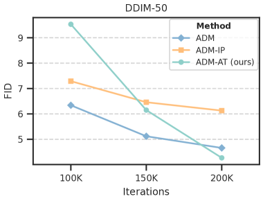
Figure 2: The convergence of methods trained from scratch on CIFAR-10 $32\times 32$. We use the DDIM sampler with 50 NFEs for sampling.

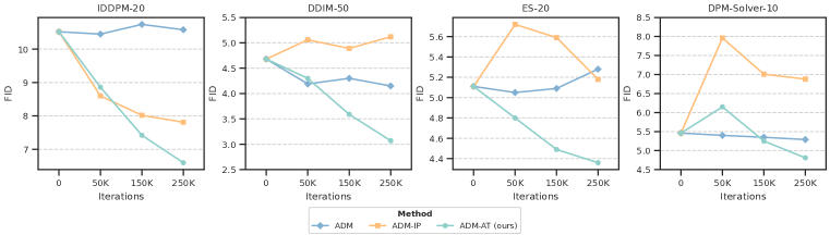
Figure 3: The convergence of methods fine-tuned from a same pretrained model on CIFAR-10 $32\times 32$. We compare the performance of methods on various samplers.

In classification tasks, adding adversarial perturbations usually slows the convergence of model training (Zhu et al., 2020). We are interested to see whether AT also affects the convergence of the diffusion training process.

Firstly, we explore the convergence of models trained from scratch. We utilize DDIM as the sampler with 50 NFEs and the results are shown in Figure 2. We observe that our AT method and ADM-IP exhibit slower convergence compared to ADM at the beginning (before 100K iterations), while as training more iterations (200K), our AT method shows a notable advantage.

Moreover, we explore the convergence of models under fine-tuning setting and the results are shown in Figure 3. We observe under this setting, when given a pretrained diffusion model like ADM, fine-tuning it with our proposed AT improves performance faster than other baselines. Overall, we observe that incorporating AT with a diffusion framework does not affect the convergence of the model much, especially in the fine-tuning setting.

G.3 More Ablation Study

Table 15: Comparison of different adversarial learning rate $\alpha$ of our AT framework on CIFAR10 32x32. IDDPM is adopted as the inference sampler.

$\alpha$ $\backslash$ NFEs	5	8	10	20	50
$\alpha=0.05$	51.72	32.09	25.48	10.38	4.36
$\alpha=0.1$	37.15	23.59	15.88	6.60	3.34
$\alpha=0.5$	63.73	40.08	27.57	7.23	3.42

Table 16: Comparison of different adversarial learning rate $\alpha$ of our AT framrwork on ImageNet 64x64. IDDPM is adopted as the inference sampler.

$\alpha$ $\backslash$ NFEs	5	8	10	20	50
$\alpha=0.1$	56.92	27.39	24.06	10.17	5.82
$\alpha=0.5$	45.65	23.79	19.18	8.28	4.01
$\alpha=0.8$	46.92	28.46	22.47	9.70	4.25

Ablation on $\alpha$

We investigate the impact of adversarial learning rate $\alpha$ in our framework. The results of various $\alpha$ on CIFAR10 32x32 and ImageNet 64x64 are shown in Table 15 and Table 16, respectively. We observe that $\alpha$ set to 0.1 is better on CIFAR10 32x32 and $\alpha=0.5$ is better for ImageNet 64x64. That says, the image in larger size corresponds to larger optimal perturbation level $\alpha$. We speculate this is because we use the perturbation measured under $\ell_{2}$-norm, where the $\ell_{2}$-norm of vector will increase with its dimension.

Table 17: Comparison of different perturbation norms ($l_{1}$, $l_{2}$ $l_{\infty}$) of our AT framework on CIFAR10 32x32.

Perturbation Norm	IDDPM-50	DDIM-50	ES-20	DPM-Solver-10
$l_{1}$	4.45	4.91	4.72	5.05
$l_{2}$	3.34	3.07	4.36	4.81
$l_{\infty}$	3.87	3.63	4.48	5.32

Ablation on perturbation norm

During our experiments, we adopt $\ell_{2}$-adversarial perturbation. Actually, perturbations in Euclidean space under different $\ell_{p}$ norm are equivalent with each other, e.g., for vector $\boldsymbol{\delta}\in\mathbb{R}^{d}$, it holds $\|\boldsymbol{\delta}\|_{\infty}\leq\|\boldsymbol{\delta}\|_{2}\leq\sqrt{d}\|\boldsymbol{\delta}\|_{\infty}$. Therefore, we select $\|\cdot\|_{2}$ as representation in our paper. Next, we explore the proposed ADM-AT under different adversarial perturbations.

The results are in Table 17. We found that our method under $\ell_{2}$-perturbation is more stable and indeed has better performance, thus we suggest to use $\ell_{2}$-perturbation as in the main body of this paper.

G.4 Qualitative Comparisons

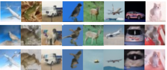
Figure 4: The qualitative comparsions of ADM-AT (top, FID 6.60), ADM-IP (middle, FID 7.81), and ADM (bottom, FID 10.58) on CIFAR10 $32\times 32$. We use the IDDPM sampler with 20 NFEs for sampling.

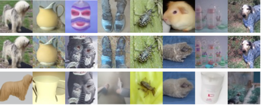
Figure 5: The qualitative comparsions of ADM-AT (top, FID 6.20), ADM-IP (middle, FID 8.40) and ADM (bottom, FID 8.32) on ImageNet $64\times 64$. We use the DDIM sampler with 20 NFEs for sampling.

Figure 6: The qualitative comparsions of LCM (left) and LCM-AT (right) with one-step generation. The text prompt is A photo of beautiful mountain with realistic sunset and blue lake, highly detailed, masterpiece.

Figure 7: The qualitative comparsions of LCM (left) and LCM-AT (right) with one-step generation. The text prompt is Astronaut in a jungle, cold color palette, muted colors, detailed, 8k.

Figure 4, 5, 6, 7 show the qualitative comparisons between our proposed AT method and baselines. Our proposed AT method generates more realistic and higher-fidelity samples. We attribute this to our AT algorithm mitigates the distribution mismatch problem.

References

- Bao et al. (2022) Fan Bao, Chongxuan Li, Jun Zhu, and Bo Zhang. Analytic-dpm: an analytic estimate of the optimal reverse variance in diffusion probabilistic models. In International Conference on Learning Representations, 2022.
- Bengio et al. (2015) Samy Bengio, Oriol Vinyals, Navdeep Jaitly, and Noam Shazeer. Scheduled sampling for sequence prediction with recurrent neural networks. In Advances in Neural Information Processing Systems, 2015.
- Blattmann et al. (2023) Andreas Blattmann, Robin Rombach, Huan Ling, Tim Dockhorn, Seung Wook Kim, Sanja Fidler, and Karsten Kreis. Align your latents: High-resolution video synthesis with latent diffusion models. In Conference on Computer Vision and Pattern Recognition, 2023.
- Chen et al. (2023) Hongrui Chen, Holden Lee, and Jianfeng Lu. Improved analysis of score-based generative modeling: User-friendly bounds under minimal smoothness assumptions. In International Conference on Machine Learning, 2023.
- Chen et al. (2024) Junsong Chen, Jincheng Yu, Chongjian Ge, Lewei Yao, Enze Xie, Zhongdao Wang, James T. Kwok, Ping Luo, Huchuan Lu, and Zhenguo Li. Pixart-: Fast training of diffusion transformer for photorealistic text-to-image synthesis. In International Conference on Learning Representations, 2024.
- Chen et al. (2022) Sitan Chen, Sinho Chewi, Jerry Li, Yuanzhi Li, Adil Salim, and Anru Zhang. Sampling is as easy as learning the score: theory for diffusion models with minimal data assumptions. In International Conference on Learning Representations, 2022.
- Deng et al. (2009) Jia Deng, Wei Dong, Richard Socher, Li-Jia Li, Kai Li, and Li Fei-Fei. Imagenet: A large-scale hierarchical image database. In Conference on Computer Vision and Pattern Recognition, 2009.
- Dhariwal & Nichol (2021) Prafulla Dhariwal and Alexander Quinn Nichol. Diffusion models beat GANs on image synthesis. In Advances in Neural Information Processing Systems, volume 34, pp. 8780–8794, 2021.
- Duchi (2016) John Duchi. Lecture notes for statistics 311/electrical engineering 377. URL: https://stanford. edu/class/stats311/Lectures/full_notes. pdf. Last visited on, 2:23, 2016.
- Goodfellow et al. (2014) Ian J Goodfellow, Jean Pouget-Abadie, Mehdi Mirza, Bing Xu, David Warde-Farley, Sherjil Ozair, Aaron C Courville, and Yoshua Bengio. Generative adversarial nets. In Advances in Neural Information Processing Systems, 2014.
- Goodfellow et al. (2015) Ian J. Goodfellow, Jonathon Shlens, and Christian Szegedy. Explaining and harnessing adversarial examples. In International Conference on Learning Representations, 2015.
- He et al. (2016) Kaiming He, Xiangyu Zhang, Shaoqing Ren, and Jian Sun. Deep residual learning for image recognition. In Conference on Computer Vision and Pattern Recognition, 2016.
- Hessel et al. (2021) Jack Hessel, Ari Holtzman, Maxwell Forbes, Ronan Le Bras, and Yejin Choi. Clipscore: A reference-free evaluation metric for image captioning. In Proceedings of the Conference on Empirical Methods in Natural Language Processing,, 2021.
- Heusel et al. (2017) Martin Heusel, Hubert Ramsauer, Thomas Unterthiner, Bernhard Nessler, and Sepp Hochreiter. Gans trained by a two time-scale update rule converge to a local nash equilibrium. 2017.
- Ho et al. (2020) Jonathan Ho, Ajay Jain, and Pieter Abbeel. Denoising diffusion probabilistic models. In Advances in Neural Information Processing Systems, 2020.
- Ho et al. (2022a) Jonathan Ho, Chitwan Saharia, William Chan, David J Fleet, Mohammad Norouzi, and Tim Salimans. Cascaded diffusion models for high fidelity image generation. Journal of Machine Learning Research, 23(47):1–33, 2022a.
- Ho et al. (2022b) Jonathan Ho, Tim Salimans, Alexey Gritsenko, William Chan, Mohammad Norouzi, and David J Fleet. Video diffusion models. In Advances in Neural Information Processing Systems, 2022b.
- Jiang et al. (2020) Haoming Jiang, Pengcheng He, Weizhu Chen, Xiaodong Liu, Jianfeng Gao, and Tuo Zhao. SMART: robust and efficient fine-tuning for pre-trained natural language models through principled regularized optimization. In Proceedings of the 58th Annual Meeting of the Association for Computational Linguistics, 2020.
- Kingma & Welling (2013) Diederik P Kingma and Max Welling. Auto-encoding variational Bayes. In International Conference on Learning Representations, 2013.
- Krizhevsky & Hinton (2009) Alex Krizhevsky and Geoffrey Hinton. Learning multiple layers of features from tiny images. 2009.
- Lee & Raginsky (2018) Jaeho Lee and Maxim Raginsky. Minimax statistical learning with wasserstein distances. In Advances in Neural Information Processing Systems, 2018.
- Li et al. (2023) Gen Li, Yuting Wei, Yuxin Chen, and Yuejie Chi. Towards faster non-asymptotic convergence for diffusion-based generative models. Preprint arXiv:2306.09251, 2023.
- Li et al. (2024) Mingxiao Li, Tingyu Qu, Wei Sun, and Marie-Francine Moens. Alleviating exposure bias in diffusion models through sampling with shifted time steps. In International Conference on Learning Representations, 2024.
- Li & van der Schaar (2024) Yangming Li and Mihaela van der Schaar. On error propagation of diffusion models. In The Twelfth International Conference on Learning Representations, 2024.
- Lin et al. (2014a) Tsung-Yi Lin, Michael Maire, Serge Belongie, James Hays, Pietro Perona, Deva Ramanan, Piotr Dollár, and C Lawrence Zitnick. Microsoft coco: Common objects in context. In Computer Vision–ECCV 2014: 13th European Conference, Zurich, Switzerland, September 6-12, 2014, Proceedings, Part V 13, 2014a.
- Lin et al. (2014b) Tsung-Yi Lin, Michael Maire, Serge J. Belongie, James Hays, Pietro Perona, Deva Ramanan, Piotr Dollár, and C. Lawrence Zitnick. Microsoft COCO: common objects in context. In ECCV, 2014b.
- Loshchilov & Hutter (2019) Ilya Loshchilov and Frank Hutter. Decoupled weight decay regularization. In International Conference on Learning Representations, 2019.
- Lou & Ermon (2023) Aaron Lou and Stefano Ermon. Reflected diffusion models. In International Conference on Machine Learning, 2023.
- Lu et al. (2022a) Cheng Lu, Yuhao Zhou, Fan Bao, Jianfei Chen, Chongxuan Li, and Jun Zhu. Dpm-solver: A fast ode solver for diffusion probabilistic model sampling in around 10 steps. In Advances in Neural Information Processing Systems, 2022a.
- Lu et al. (2022b) Cheng Lu, Yuhao Zhou, Fan Bao, Jianfei Chen, Chongxuan LI, and Jun Zhu. Dpm-solver: A fast ode solver for diffusion probabilistic model sampling in around 10 steps. In Advances in Neural Information Processing Systems, 2022b.
- Luo et al. (2023) Simian Luo, Yiqin Tan, Longbo Huang, Jian Li, and Hang Zhao. Latent consistency models: Synthesizing high-resolution images with few-step inference, 2023.
- Ma et al. (2024) Jiajun Ma, Shuchen Xue, Tianyang Hu, Wenjia Wang, Zhaoqiang Liu, Zhenguo Li, Zhi-Ming Ma, and Kenji Kawaguchi. The surprising effectiveness of skip-tuning in diffusion sampling. arXiv preprint arXiv:2402.15170, 2024.
- Madry et al. (2018) Aleksander Madry, Aleksandar Makelov, Ludwig Schmidt, Dimitris Tsipras, and Adrian Vladu. Towards deep learning models resistant to adversarial attacks. In International Conference on Learning Representations, 2018.
- Namkoong (2019) Hongseok Namkoong. Reliable machine learning via distributional robustness. PhD thesis, Stanford University, 2019.
- (35) Alexander Quinn Nichol, Prafulla Dhariwal, Aditya Ramesh, Pranav Shyam, Pamela Mishkin, Bob McGrew, Ilya Sutskever, and Mark Chen. GLIDE: towards photorealistic image generation and editing with text-guided diffusion models. In International Conference on Machine Learning.
- Nie et al. (2022) Weili Nie, Brandon Guo, Yujia Huang, Chaowei Xiao, Arash Vahdat, and Animashree Anandkumar. Diffusion models for adversarial purification. In International Conference on Machine Learning, 2022.
- Ning et al. (2023) Mang Ning, Enver Sangineto, Angelo Porrello, Simone Calderara, and Rita Cucchiara. Input perturbation reduces exposure bias in diffusion models. In International Conference on Machine Learning, 2023.
- Ning et al. (2024) Mang Ning, Mingxiao Li, Jianlin Su, Albert Ali Salah, and Itir Önal Ertugrul. Elucidating the exposure bias in diffusion models. In International Conference on Learning Representations, 2024.
- Radford et al. (2019) Alec Radford, Jeffrey Wu, Rewon Child, David Luan, Dario Amodei, Ilya Sutskever, et al. Language models are unsupervised multitask learners. OpenAI blog, 1(8):9, 2019.
- Ramesh et al. (2022) Aditya Ramesh, Prafulla Dhariwal, Alex Nichol, Casey Chu, and Mark Chen. Hierarchical text-conditional image generation with clip latents, 2022.
- Ranzato et al. (2016) Marc’Aurelio Ranzato, Sumit Chopra, Michael Auli, and Wojciech Zaremba. Sequence level training with recurrent neural networks. In International Conference on Learning Representations, 2016.
- Ravuri & Vinyals (2019) Suman V. Ravuri and Oriol Vinyals. Classification accuracy score for conditional generative models. In Advances in Neural Information Processing Systems, 2019.
- Rebuffi et al. (2021) Sylvestre-Alvise Rebuffi, Sven Gowal, Dan A. Calian, Florian Stimberg, Olivia Wiles, and Timothy A. Mann. Fixing data augmentation to improve adversarial robustness. Preprint arXiv:2103.01946, 2021.
- Ren et al. (2024) Zhiyao Ren, Yibing Zhan, Liang Ding, Gaoang Wang, Chaoyue Wang, Zhongyi Fan, and Dacheng Tao. Multi-step denoising scheduled sampling: Towards alleviating exposure bias for diffusion models. In AAAI Conference on Artificial Intelligence, 2024.
- Rennie et al. (2017) Steven J. Rennie, Etienne Marcheret, Youssef Mroueh, Jerret Ross, and Vaibhava Goel. Self-critical sequence training for image captioning. In IEEE Conference on Computer Vision and Pattern Recognition, 2017.
- Rombach et al. (2022) Robin Rombach, Andreas Blattmann, Dominik Lorenz, Patrick Esser, and Björn Ommer. High-resolution image synthesis with latent diffusion models. In Conference on Computer Vision and Pattern Recognition, 2022.
- Ronneberger et al. (2015) Olaf Ronneberger, Philipp Fischer, and Thomas Brox. U-net: Convolutional networks for biomedical image segmentation. In Medical Image Computing and Computer-Assisted Intervention–MICCAI 2015: 18th International Conference, Munich, Germany, October 5-9, 2015, Proceedings, Part III 18, pp. 234–241. Springer, 2015.
- Saharia et al. (2022) Chitwan Saharia, William Chan, Saurabh Saxena, Lala Li, Jay Whang, Emily L Denton, Kamyar Ghasemipour, Raphael Gontijo Lopes, Burcu Karagol Ayan, Tim Salimans, Jonathan Ho, David J Fleet, and Mohammad Norouzi. Photorealistic text-to-image diffusion models with deep language understanding. In Advances in Neural Information Processing Systems, 2022.
- Salimans & Ho (2022) Tim Salimans and Jonathan Ho. Progressive distillation for fast sampling of diffusion models. In International Conference on Learning Representations, 2022.
- Schuhmann et al. (2022) Christoph Schuhmann, Romain Beaumont, Richard Vencu, Cade Gordon, Ross Wightman, Mehdi Cherti, Theo Coombes, Aarush Katta, Clayton Mullis, Mitchell Wortsman, Patrick Schramowski, Srivatsa Kundurthy, Katherine Crowson, Ludwig Schmidt, Robert Kaczmarczyk, and Jenia Jitsev. LAION-5B: an open large-scale dataset for training next generation image-text models. In Advances in Neural Information Processing Systems, 2022.
- Shafahi et al. (2019) Ali Shafahi, Mahyar Najibi, Amin Ghiasi, Zheng Xu, John P. Dickerson, Christoph Studer, Larry S. Davis, Gavin Taylor, and Tom Goldstein. Adversarial training for free! In Advances in Neural Information Processing Systems 32: Annual Conference on Neural Information Processing Systems 2019, NeurIPS 2019, December 8-14, 2019, Vancouver, BC, Canada, 2019.
- Shapiro (2017) Alexander Shapiro. Distributionally robust stochastic programming. SIAM Journal on Optimization, 27(4):2258–2275, 2017.
- Shen et al. (2016) Shiqi Shen, Yong Cheng, Zhongjun He, Wei He, Hua Wu, Maosong Sun, and Yang Liu. Minimum risk training for neural machine translation. In Proceedings of the 54th Annual Meeting of the Association for Computational Linguistics, 2016.
- Shiryaev (2016) Albert N Shiryaev. Probability-1, volume 95. Springer, 2016.
- Sinha et al. (2018) Aman Sinha, Hongseok Namkoong, and John Duchi. Certifying some distributional robustness with principled adversarial training. In International Conference on Learning Representations, 2018.
- Sohl-Dickstein et al. (2015) Jascha Sohl-Dickstein, Eric Weiss, Niru Maheswaranathan, and Surya Ganguli. Deep unsupervised learning using nonequilibrium thermodynamics. In International Conference on Machine Learning, 2015.
- Song et al. (2022) Jiaming Song, Chenlin Meng, and Stefano Ermon. Denoising diffusion implicit models. In International Conference on Learning Representations, 2022.
- Song et al. (2020) Yang Song, Jascha Sohl-Dickstein, Diederik P Kingma, Abhishek Kumar, Stefano Ermon, and Ben Poole. Score-based generative modeling through stochastic differential equations. In International Conference on Learning Representations, 2020.
- Song et al. (2021) Yang Song, Conor Durkan, Iain Murray, and Stefano Ermon. Maximum likelihood training of score-based diffusion models. 2021.
- Song et al. (2023) Yang Song, Prafulla Dhariwal, Mark Chen, and Ilya Sutskever. Consistency models. In International Conference on Machine Learning, 2023.
- Villani et al. (2009) Cédric Villani et al. Optimal transport: old and new, volume 338. Springer, 2009.
- Wainwright (2019) Martin J Wainwright. High-dimensional statistics: A non-asymptotic viewpoint, volume 48. Cambridge university press, 2019.
- Wang et al. (2022) Ruoyu Wang, Mingyang Yi, Zhitang Chen, and Shengyu Zhu. Out-of-distribution generalization with causal invariant transformations. In Conference on Computer Vision and Pattern Recognition, 2022.
- Wang et al. (2023) Zekai Wang, Tianyu Pang, Chao Du, Min Lin, Weiwei Liu, and Shuicheng Yan. Better diffusion models further improve adversarial training. In International Conference on Machine Learning, 2023.
- Wu et al. (2020) Dongxian Wu, Shu-Tao Xia, and Yisen Wang. Adversarial weight perturbation helps robust generalization. In Advances in Neural Information Processing Systems, 2020.
- Xue et al. (2024a) Shuchen Xue, Zhaoqiang Liu, Fei Chen, Shifeng Zhang, Tianyang Hu, Enze Xie, and Zhenguo Li. Accelerating diffusion sampling with optimized time steps. arXiv preprint arXiv:2402.17376, 2024a.
- Xue et al. (2024b) Shuchen Xue, Mingyang Yi, Weijian Luo, Shifeng Zhang, Jiacheng Sun, Zhenguo Li, and Zhi-Ming Ma. Sa-solver: Stochastic adams solver for fast sampling of diffusion models. Advances in Neural Information Processing Systems, 36, 2024b.
- Yi et al. (2021) Mingyang Yi, Lu Hou, Jiacheng Sun, Lifeng Shang, Xin Jiang, Qun Liu, and Zhiming Ma. Improved ood generalization via adversarial training and pretraing. In International Conference on Machine Learning, 2021.
- Yi et al. (2023a) Mingyang Yi, Jiacheng Sun, and Zhenguo Li. On the generalization of diffusion model. Preprint arXiv:2305.14712, 2023a.
- Yi et al. (2023b) Mingyang Yi, Ruoyu Wang, Jiacheng Sun, Zhenguo Li, and Zhi-Ming Ma. Breaking correlation shift via conditional invariant regularizer. In The International Conference on Learning Representations, 2023b.
- Yi et al. (2024) Mingyang Yi, Aoxue Li, Yi Xin, and Zhenguo Li. Towards understanding the working mechanism of text-to-image diffusion model. Preprint arXiv:2405.15330, 2024.
- Yin et al. (2024) Tianwei Yin, Michaël Gharbi, Richard Zhang, Eli Shechtman, Frédo Durand, William T Freeman, and Taesung Park. One-step diffusion with distribution matching distillation. In CVPR, 2024.
- Zhang et al. (2023) Boya Zhang, Weijian Luo, and Zhihua Zhang. Enhancing adversarial robustness via score-based optimization. In Advances in Neural Information Processing Systems, 2023.
- Zhang et al. (2019a) Dinghuai Zhang, Tianyuan Zhang, Yiping Lu, Zhanxing Zhu, and Bin Dong. You only propagate once: Accelerating adversarial training via maximal principle. In Advances in Neural Information Processing Systems, 2019a.
- Zhang et al. (2019b) Hongyang Zhang, Yaodong Yu, Jiantao Jiao, Eric P. Xing, Laurent El Ghaoui, and Michael I. Jordan. Theoretically principled trade-off between robustness and accuracy. In International Conference on Machine Learning, 2019b.
- Zhang et al. (2019c) Wen Zhang, Yang Feng, Fandong Meng, Di You, and Qun Liu. Bridging the gap between training and inference for neural machine translation. In Proceedings of the 57th Conference of the Association for Computational Linguistics, 2019c.
- Zhu et al. (2020) Chen Zhu, Yu Cheng, Zhe Gan, Siqi Sun, Tom Goldstein, and Jingjing Liu. Freelb: Enhanced adversarial training for natural language understanding. In International Conference on Learning Representations, 2020.