Erwin: A Tree-based Hierarchical Transformer for Large-scale Physical Systems

Abstract

Large-scale physical systems defined on irregular grids pose significant scalability challenges for deep learning methods, especially in the presence of long-range interactions and multi-scale coupling. Traditional approaches that compute all pairwise interactions, such as attention, become computationally prohibitive as they scale quadratically with the number of nodes. We present Erwin, a hierarchical transformer inspired by methods from computational many-body physics, which combines the efficiency of tree-based algorithms with the expressivity of attention mechanisms. Erwin employs ball tree partitioning to organize computation, which enables linear-time attention by processing nodes in parallel within local neighborhoods of fixed size. Through progressive coarsening and refinement of the ball tree structure, complemented by a novel cross-ball interaction mechanism, it captures both fine-grained local details and global features. We demonstrate Erwin’s effectiveness across multiple domains, including cosmology, molecular dynamics, and particle fluid dynamics, where it consistently outperforms baseline methods both in accuracy and computational efficiency.

Figure 1: Top: Ball tree attention over a molecular graph. Multi-head self-attention (MHSA) is computed in parallel at fixed hierarchy levels (bold circles). In the following layers, the tree is progressively coarsened to learn global features, while the partition size is fixed. Bottom: Computational advantages of our model.

1 Introduction

Scientific deep learning is tackling increasingly computationally intensive tasks, following the trajectory of computer vision and natural language processing. Applications range from molecular dynamics (MD) (Arts et al., 2023), computational particle mechanics (Alkin et al., 2024b), to weather forecasting (Bodnar et al., 2024), where simulations often involve data defined on irregular grids with thousands to millions of nodes, depending on the required resolution and complexity of the system.

Such large-scale systems pose a significant challenge to existing methods that were developed and validated at smaller scales. For example, in computational chemistry, models are typically trained on molecules with tens of atoms (Kovács et al., 2023), while molecular dynamics simulations can involve well beyond thousands of atoms. This scale disparity might result in prohibitive runtimes that render models inapplicable in high-throughput scenarios such as protein design (Watson et al., 2023) or screening (Fu et al., 2022).

A key challenge in scaling to larger system sizes is that computational methods which work well at small scales break down at larger scales. For small systems, all pairwise interactions can be computed explicitly, allowing deep learning models to focus on properties like equivariance (Cohen & Welling, 2016). However, this brute-force approach becomes intractable as the system size grows. At larger scales, approximations are required to efficiently capture both long-range effects from slowly decaying potentials or multi-scale coupling (Majumdar et al., 2020). As a result, models validated only on small systems often lack the architectural components necessary for efficient scaling.

This problem has been extensively studied in computational many-body physics (Hockney & Eastwood, 2021), where the need for evaluating long-range potentials for large-scale particle systems led to the development of sub-quadratic tree-based algorithms (Barnes & Hut, 1986; Carrier et al., 1988). These methods are based on the intuition that distant particles can be approximated through their mean field effect rather than individual interactions (Pfalzner & Gibbon, 1996). The computation then is structured using hierarchical trees to efficiently organize the computation at multiple scales. While highly popular for numerical simulations, these tree-based methods have seen limited adoption in deep learning due to poor synergy with GPU architectures.

Transformers (Vaswani et al., 2017), on the other hand, employ the highly optimized attention mechanism, which comes with the quadratic cost of computing all-to-all interactions. In this work, we combine the efficiency of hierarchical tree methods with the expressivity of attention to create a scalable architecture for the processing of large-scale particle systems. Our approach leverages ball trees to organize computation at multiple scales, enabling both local accuracy and global feature capture while maintaining linear complexity in the number of nodes.

The main contributions of the work are the following:

• We introduce ball tree partitioning for efficient point cloud processing, enabling linear-time self-attention through localized computation within balls at different hierarchical levels.

• We present Erwin, a hierarchical transformer that processes data through progressive coarsening and refinement of ball tree structures, effectively capturing both fine-grained local interactions and global features while maintaining computational efficiency.

• We validate Erwin’s performance across multiple large-scale physical domains:

  • Capturing long-range interactions (cosmology)

  • Computational efficiency (molecular dynamics)

  • Model expressivity on large-scale multi-scale phenomena (turbulent fluid dynamics)

  achieving state-of-the-art performance in both computational efficiency and prediction accuracy.

2 Related Works: sub-quadratic attention

One way to avoid the quadratic cost of self-attention is to linearize attention by performing it on non-overlapping patches. For data on regular grids, like images, the SwinTransformer (Liu et al., 2021) achieves this by limiting attention to local windows with cross-window connection enabled by shifting the windows. However, for irregular data such as point clouds or non-uniform meshes, one first needs to induce a structure that will allow for patching. Several approaches (Liu et al., 2023; Sun et al., 2022) transform point clouds into sequences, most notably, PointTransformer v3 (Wu et al., 2024), which projects points into voxels and orders them using space-filling curves (e.g., Hilbert curve). While scalable, these curves introduce artificial discontinuities that can break local spatial relationships.

Particularly relevant to our work are hierarchical attention methods. In the context of 1D sequences, approaches like the H-transformer (Zhu & Soricut, 2021) and Fast Multipole Attention (Kang et al., 2023) approximate self-attention through multi-level decomposition: tokens interact at full resolution locally while distant interactions are computed using learned or fixed groupings at progressively coarser scales. For point clouds, OctFormer (Wang, 2023) converts spatial data into a sequence by traversing an octree, ensuring spatially adjacent points are consecutive in memory. While conceptually similar to our approach, OctFormer relies on computationally expensive octree convolutions, whereas our utilization of ball trees leads to significant efficiency gains.

Rather than using a hierarchical decomposition, another line of work proposes cluster attention (Janny et al., 2023; Alkin et al., 2024a). These methods first group points into clusters and aggregate their features at the cluster centroids through message passing or cross-attention. After computing attention between the centroids, the updated features are then distributed back to the original points. While these approaches achieve the quadratic cost only in the number of clusters, they introduce an information bottleneck at the clustering step that may sacrifice fine-grained details and fail to capture features at multiple scales - a limitation our hierarchical approach aims to overcome.

3 Background

Our work revolves around attention, which we aim to linearize by imposing structure onto point clouds using ball trees. We formally introduce both concepts in this section.

3.1 Attention

The standard self-attention mechanism is based on the scaled dot-product attention (Vaswani et al., 2017). Given a set $X$ of $N$ input feature vectors of dimension $C$, self-attention is computed as

$$\begin{gathered}\mathbf{Q},\>\mathbf{K},\>\mathbf{V}=\mathbf{XW}_{q},\>\mathbf{XW}_{k},\>\mathbf{XW}_{v}\\ \mathrm{Att}(\mathbf{Q},\mathbf{K},\mathbf{V})=\text{softmax}\left(\frac{\mathbf{QK}^{T}}{\sqrt{C^{\prime}}}+\mathcal{B}\right)\>\mathbf{V}\end{gathered}$$ (1)

where $\mathbf{W}_{q},\mathbf{W}_{k},\mathbf{W}_{v}\in\mathbb{R}^{C\times C^{\prime}}$ are learnable weights and $\mathcal{B}\in\mathbb{R}^{N\times N}$ is the bias term.

Multi-head self-attention (MHSA) improves expressivity by computing attention $H$ times with different weights and concatenating the output before the final projection:

$$\begin{gathered}\mathrm{MHSA}(\mathbf{X})=[\mathbf{Y}_{1},\cdots,\mathbf{Y}_{H}]\>\mathbf{W}^{O}\\ \mathbf{Y}_{i}=\mathrm{Att}(\mathbf{X}\mathbf{W}_{q}^{i},\mathbf{X}\mathbf{W}_{k}^{i},\mathbf{X}\mathbf{W}_{v}^{i})\end{gathered}$$ (2)

where $[\cdot,\cdots,\cdot]$ denotes concatenation along the feature dimension, and $\mathbf{W}^{i}_{q},\mathbf{W}^{i}_{k},\mathbf{W}^{i}_{v}\in\mathbb{R}^{C\times(C^{\prime}/H)}$ and $\mathbf{W}^{O}\in\mathbb{R}^{C\times C^{\prime}}$ are learnable weights.

The operator explicitly computes interactions between all elements in the input set without any locality constraints. This yields the quadratic computational cost w.r.t. the input set size $\mathcal{O}(N^{2})$. Despite being heavily optimized (Dao, 2024), this remains a bottleneck for large-scale applications.

3.2 Ball tree

A ball tree is a hierarchical data structure that recursively partitions points into nested sets of equal size, where each set is represented by a ball that covers all the points in the set. Assume we operate on the $d$-dim. Euclidean space $\left(\mathbb{R}^{d},||\cdot||_{2}\right)$ where we have a point cloud (set) $P=\{\mathbf{p}_{1},...,\mathbf{p}_{n}\}\subset\mathbb{R}^{d}$.

Definition 3.1 (Ball).

A ball is a region bounded by a hypersphere in $\mathbb{R}^{d}$. Each ball is represented by the coordinates of its center $\mathbf{c}\in\mathbb{R}^{d}$ and radius $r\in\mathbb{R}_{+}$:

$$B=B(\mathbf{c},r)=\{\mathbf{z}\in\mathbb{R}^{d}\mid||\mathbf{z}-\mathbf{c}||_{2}\leq r\}.$$ (3)

We will omit the parameters $(\mathbf{c},r)$ for brevity from now on.

Definition 3.2 (Ball Tree).

A ball tree $T$ on point set $P$ is a hierarchical sequence of partitions $\{L_{0},L_{1},...,L_{m}\}$, where each level $L_{i}$ consists of disjoint balls that cover $P$. At the leaf level $i=0$, the nodes are the original points:

$$L_{0}=\{\{\mathbf{p}_{j}\}\mid\mathbf{p}_{j}\in P\}$$

For each subsequent level $i>0$, each ball $B\in L_{i}$ is formed by merging two balls at the previous level $B_{1},B_{2}\in L_{i-1}$:

$$L_{i}=\{\{B_{1}\cup B_{2}\}\mid B_{1},B_{2}\in L_{i-1}\}$$ (4)

such that its center is computed as the center of mass:

$$\mathbf{c}_{B}=\frac{|B_{1}|\mathbf{c}_{1}+|B_{2}|\mathbf{c}_{2}}{|B_{1}|+|B_{2}|}$$

and its radius is determined by the furthest point it contains:

$$r_{B}=max\{||\mathbf{p}-\mathbf{c}_{B}||_{2}\mid\mathbf{p}\in B_{1}\cup B_{2}\}\vskip-5.0pt$$

where $|B|$ denotes the number of points contained in $B$.

To construct the ball tree, we recursively split the data points into two sets starting from $P$. In each recursive step, we find the dimension of the largest spread (i.e. the $\text{max}-\text{min}$ value) and split at its median (Pedregosa et al., 2012), constructing covering balls per Def.3.2. For details, see Appendix Alg.1.

Tree Completion

To enable efficient implementation, we want to work with perfect binary trees, i.e. trees where all internal nodes have exactly two children and all leaf nodes appear at the same depth. To achieve this, we pad the leaf level of a ball tree with virtual nodes, yielding the total number of nodes $2^{m}$, where $m=\text{ceil}(\log_{2}(n))$.

3.2.1 Ball tree properties

In the context of our method, there are several properties of ball trees that enable efficient hierarchical partitioning:

Proposition 3.3 (Ball Tree Properties).

The ball tree $T$ constructed as described satisfies the following properties:

1. The tree is a perfect binary tree.

2. At each level $i$, each ball contains exactly $2^{i}$ leaf nodes.

3. Balls at each level cover the point set

   $$\bigcup_{B\in L_{i}}B=P\quad\forall i\in\{0,...,m\}.$$

Proposition 3.4 (Contiguous Storage).

For a ball tree $T=\{L_{0},L_{1},...,L_{m}\}$ on point cloud $P=\{\mathbf{p}_{1},...,\mathbf{p}_{n}\}$, there exists a bijective mapping $\pi:\{1,...,n\}\rightarrow\{1,...,n\}$ such that points belonging to the same ball $B\in L_{i}$ have contiguous indices under $\pi$.

As a corollary, the hierarchical structure at each level can be represented by nested intervals of contiguous indices:

Example.

Let $P=\{\mathbf{p}_{1},...,\mathbf{p}_{8}\}$, then a ball tree $T=\{L_{0},L_{1},L_{2},L_{3}\}$ is stored after the permutation $\pi$ as

$$L_{3}\hskip 35.0pt \overbracket{\hskip 118.0pt}$$

$$L_{2}\hskip 35.0pt \overbracket{\hskip 53.5pt}\overbracket{\hskip 63.0pt}$$

$$L_{1}\hskip 35.0pt \overbracket{\hskip 28.0pt}\overbracket{\hskip 28.5pt}\overbracket{\hskip 28.5pt}\overbracket{\hskip 28.5pt}$$

$$L_{0}=\pi(P)\hskip 14.0pt \hskip 3.0pt\mathbf{p}_{a}\hskip 4.0pt\mathbf{p}_{b}\hskip 5.0pt\mathbf{p}_{c}\hskip 4.0pt\mathbf{p}_{d}\hskip 5.0pt\mathbf{p}_{e}\hskip 4.0pt\mathbf{p}_{f}\hskip 5.0pt\mathbf{p}_{g}\hskip 4.0pt\mathbf{p}_{h}$$

The contiguous storage property, combined with the fixed size of balls at each level, enables efficient implementation through tensor operations. Specifically, accessing any ball $B\in L_{i}$ simply requires selecting a contiguous sequence of $2^{i}$ indices. For instance, in the example above, for $i=2$, we select a:d and e:h to access the balls. Since the balls are equal, we can simply reshape $L_{0}$ to access any level. This representation makes it particularly efficient to implement our framework’s core operations - ball attention and coarsening/refinement - which we will introduce next.

Another important property of ball trees is that while they cover the whole point set, they are not required to partition the entire space. Coupled with completeness, it means that at each tree level, the nodes are essentially associated with the same scale. This contrasts with other structures such as oct-trees that cover the entire space and whose nodes at the same level can be associated with regions of different sizes:

Figure 2: Ball tree vs Oct-tree construction. Colors highlight the difference in scales for nodes including the same number of points.

4 Erwin Transformer

Figure 3: Overview of Erwin. Left: A sequence of two ball attention layers with intermediate tree coarsening. In every layer, attention is computed on partitions of size $16$, which correspond to progressively higher levels of hierarchy. Center (top): Coarsening and refinement of a ball tree. Center (bottom): Building a tree on top of a rotated configuration for cross-ball interaction. Right: Architecture of Erwin.

Following the notation from the background Section 3.2, we consider a point cloud $P=\{\mathbf{p}_{1},...,\mathbf{p}_{n}\}\subset\mathbb{R}^{d}$. Additionally, each point is now endowed with a feature vector yielding a feature set $X=\{\mathbf{x}_{1},...,\mathbf{x}_{n}\}\subset\mathbb{R}^{C}$.

On top of the point cloud, we build a ball tree $T=\{L_{0},...,L_{m}\}$. We initialize $L_{\mathrm{leaf}}:=L_{0}$ to denote the current finest level of the tree. As each leaf node contains a single point, it inherits its feature vector:

$$X_{\mathrm{leaf}}=\{\mathbf{x}_{B}=\mathbf{x}_{i}\mid B=\{\mathbf{p}_{i}\}\in L_{\mathrm{leaf}}\}$$ (5)

4.1 Ball tree attention

Ball attention

For each ball attention operator, we specify a level $k$ of the ball tree where each ball $B\in L_{k}$ contains $2^{k}$ leaf nodes. The choice of $k$ presents a trade-off: larger balls capture longer-range dependencies, while smaller balls are more resource-efficient. For each ball $B\in L_{k}$, we collect the leaf nodes within B

$$\mathrm{leaves}_{B}=\{B^{\prime}\in L_{\mathrm{leaf}}\mid B^{\prime}\subset B\}$$ (6)

along with their features from $X_{\mathrm{leaf}}$

$$X_{B}=\{\mathbf{x}_{B^{\prime}}\in X_{\mathrm{leaf}}\mid B^{\prime}\in\mathrm{leaves}_{B}\}$$ (7)

We then compute self-attention independently on each ball:

$$X^{\prime}_{B}=\mathrm{BAtt}(X_{B}):=\mathrm{Att}(X_{B}\mathbf{W}_{q},X_{B}\mathbf{W}_{k},X_{B}\mathbf{W}_{v})$$ (8)

where weights are shared between balls and the output $X^{\prime}_{B}$ maintains row correspondence with $X_{B}$.

Computational cost

As attention is computed independently for each ball $B\in L_{k}$, the computational cost is reduced from quadratic to linear. Precisely, for ball attention, the complexity is $\mathcal{O}(|B|^{2}\cdot\frac{n}{|B|})$, i.e. quadratic in the ball size and linear in the number of balls:

Figure 4: For highlighted points, standard attention computes interactions with all other points in the point cloud, while ball attention only considers points within their balls.

Positional encoding

We introduce positional information to the attention layer in two ways. First, we augment the features of leaf nodes with their relative positions with respect to the ball’s center of mass (relative position embedding):

$$\text{RPE}:\qquad X_{B}=X_{B}+(P_{B}-\mathbf{c}_{B})\mathbf{W}_{\mathrm{pos}}$$ (9)

where $P_{B}$ contains positions of leaf nodes, $\mathbf{c}_{B}$ is the center of mass, and $\mathbf{W}_{\mathrm{pos}}$ is a learnable projection. This allows the layer to incorporate geometric structure within each ball.

Second, we introduce a distance-based attention bias:

$$\mathcal{B}_{B}=-\sigma^{2}||\mathbf{c}_{B^{\prime}}-\mathbf{c}_{B^{\prime\prime}}||_{2},\quad B^{\prime},B^{\prime\prime}\in\mathrm{leaves}_{B}$$ (10)

with a learnable parameter $\sigma\in\mathbb{R}$ (Wessels et al., 2024). The term decays rapidly as the distance between two nodes increases which enforces locality and helps to mitigate potential artifacts from the tree building, particularly in cases where distant points are grouped together.

Cross-ball connection

To increase the receptive field of our attention operator, we implement cross-ball connections inspired by the shifted window approach in Swin Transformer (Liu et al., 2021). There, patches are displaced diagonally by half their size to obtain two different image paTreertitioning configurations. This operation can be equivalently interpreted as keeping the patches fixed while sliding the image itself.

Following this interpretation, we rotate the point cloud and construct the second ball tree $T_{\mathrm{rot}}=\{L_{0}^{\mathrm{rot}},...,L_{m}^{\mathrm{rot}}\}$ which induces a permutation $\pi^{\mathrm{rot}}$ of leaf nodes (see Fig. 3, center). We can then compute ball attention on the rotated configuration by first permuting the features according to $\pi^{\mathrm{rot}}$, applying attention, and then permuting back:

$$X^{\prime}_{B}=\pi^{-1}_{\mathrm{rot}}\left(\mathrm{BAtt}\left(\pi_{\mathrm{rot}}\left(X_{B}\right)\right)\right)$$ (11)

By alternating between the original and rotated configurations in consecutive layers, we ensure the interaction between leaf nodes in otherwise separated balls.

Tree coarsening/refinement

For larger systems, we are interested in coarser representations to capture features at larger scales. The coarsening operation allows us to hierarchically aggregate information by pooling leaf nodes to the centers of containing balls at $l$ levels higher (see Fig. 3, top, $l=1$). Suppose the leaf level is $k$. For every ball $B\in L_{k+l}$, we concatenate features of all interior leaf nodes along with their relative positions with respect to $\mathbf{c}_{B}$ and project them to a higher-dimensional representation:

$$\vskip-2.0pt\mathbf{x}_{B}=\left(\bigoplus_{B^{\prime}\in\mathrm{leaves}_{B}}\left[\mathbf{x}_{B^{\prime}},\mathbf{c}_{B^{\prime}}-\mathbf{c}_{B}\right]\right)\mathbf{W}_{c}$$ (12)

where $\bigoplus$ denotes leaf-wise concatenation, and $\mathbf{W}_{c}\in\mathbb{R}^{C^{\prime}\times 2^{l}(C+d)}$ is a learnable projection that increases the feature dimension to maintain expressivity. After coarsening, balls at level $k+l$ become the new leaf nodes, $L_{\mathrm{leaf}}:=L_{k+l}$, with features $X_{\mathrm{leaf}}:=\{\mathbf{x}_{B}\mid B\in L_{k+l}\}$. To highlight the simplicity of our method, we provide the pseudocode:

The inverse operation, refinement, allocates information from a coarse representation back to finer scales. More precisely, for a ball $B\in L_{k}$, its features are distributed back to the nodes at level $L_{k-l}$ contained within $B$ as

$$\vskip-1.0pt\{\mathbf{x}_{B^{\prime}}\mid B^{\prime}\in L_{k-l}\}=\left[\mathbf{x}_{B},P_{B}-\mathbf{c}_{B}\right]\>\mathbf{W}_{r}$$ (13)

where $P_{B}$ contains positions of all nodes at level $k-l$ within ball $B$ with center of mass $\mathbf{c}_{B}$, and $\mathbf{W}_{r}\in\mathbb{R}^{2^{l}C\times(C^{\prime}+d)}$ is a learnable projection. After refinement, $L_{\mathrm{leaf}}$ and $X_{\mathrm{leaf}}$ are updated accordingly. In pseudocode:

4.2 Model architecture

We are now ready to describe the details of the main model to which we refer as Erwin (see Fig. 3) - a hierarchical transformer operating on ball trees.

Embedding

At the embedding phase, we first construct a ball tree on top of the input point cloud and pad the leaf layer to complete the tree, as described in Section 3.2. To capture local geometric features, we employ a small-scale MPNN, which is conceptually similar to PointTransformer’s embedding module using sparse convolution. When input connectivity is not provided (e.g. mesh), we utilize the ball tree structure for a fast nearest neighbor search.

ErwinBlock

The core building block of Erwin follows a standard pre-norm transformer structure: LayerNorm followed by ball attention with a residual connection, and a SwiGLU feed-forward network (Shazeer, 2020). For the ball attention, the size $2^{k}$ of partitions is a hyperparameter. To ensure cross-ball interaction, we alternate between the original and rotated ball tree configurations, using an even number of blocks per ErwinLayer in our experiments.

Overall architecture

Following a UNet structure (Ronneberger et al., 2015; Wu et al., 2024), Erwin processes features at multiple scales through encoder and decoder paths (Fig. 3, right). The encoder progressively coarsens the ball tree while increasing feature dimensionality to maintain expressivity. The coarsening factor is a hyperparameter that takes values that are powers of $2$. At the decoder stage, the representation is refined back to the original resolution, with skip connections from corresponding encoder levels enabling multi-scale feature integration.

5 Experiments

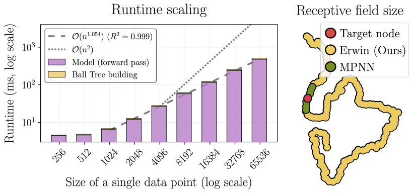
Figure 5: Left: Computational cost of Erwin. We split the total runtime into building a ball tree and running a model. The input is a batch of $16$ point clouds, each of size $n$. We fit a power law which indicates close to linear scaling. Right: Receptive field of MPNN vs Erwin, $n=800$. A node is in the receptive field if changing its features affects the target node’s output. MPNN consists of 6 layers, each node connected to $16$ nearest neighbours.

Implementation details for all experiments are given in Appendix C. The code is available at anonymized link. Extended experiments are given in Appendix B, including an additional experiment on airflow pressure modelling.

Computational cost

To experimentally evaluate Erwin’s scaling, we learn the power-law form $\mathrm{Runtime}=C\cdot n^{\beta}$ by first applying the logarithm transform to both sides and then using the least square method to evaluate $\beta$. The result is an approximately linear scaling with $\beta=1.054$ with $R^{2}=0.999$, see Fig. 5, left. Ball tree construction accounts for only a fraction of the overall time, proving the efficiency of our method for linearizing attention for point clouds.

Receptive field

One of the theoretical properties of our model is that with sufficiently many layers, its receptive field is global. To verify this claim experimentally, for an arbitrary target node, we run the forward pass of Erwin and MPNN and compute gradients of the node output with respect to all input nodes’ features. If the gradient is non-zero, the node is considered to be in the receptive field of the target node. The visualization is provided in Fig. 5, right, where we compare the receptive field of our model with that of MPNN. As expected, the MPNN has a limited receptive field, as it cannot exceed $N$ hops, where $N$ is the number of message-passing layers. Conversely, Erwin implicitly computes all-to-all interactions, enabling it to capture long-range interactions in data.

5.1 Cosmological simulations

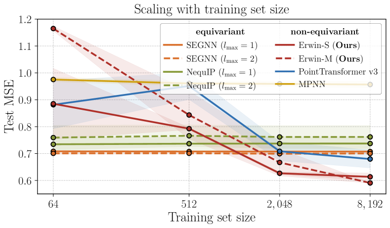
Figure 6: Test mean-squared error (MSE) on the predicted velocities as a function of training set size for the cosmology task, 5 runs per point. Point transformers indicate favourable scaling surpassing graph-based models with sufficiently many training samples.

To demonstrate our model’s ability to capture long-range interactions, we use the cosmology benchmark (Balla et al., 2024) which consists of large-scale point clouds representing potential galaxy distributions.

Dataset

The dataset is derived from N-body simulations that evolve dark matter particles from the early universe to the present time. After the simulation, gravitationally bound structures (halos) are indicated, from which the $5000$ heaviest ones are selected as potential galaxy locations. The halos form local clusters through gravity while maintaining long-range correlations that originated from interactions in the early universe before cosmic expansion, reflecting the initial conditions of simulations.

Task

The input is a point cloud $\mathbf{X}\in\mathbb{R}^{5000\times 3}$, where each row corresponds to a galaxy and column to $x,y,z$ coordinate respectively. The task is a regression problem to predict the velocity of every galaxy $\mathbf{Y}\in\mathbb{R}^{5000\times 3}$. We vary the size of the training dataset from $64$ to $8192$, while the validation and test datasets have a fixed size of $512$. The models are trained using mean squared error loss

$$\mathcal{L}=\text{MSE}(\hat{Y},Y)\vskip-2.0pt$$

between predicted and ground truth velocities.

Results

The results are shown in Fig. 6. We compare against multiple equivariant (NequIP (Batzner et al., 2021), SEGNN (Brandstetter et al., 2022)) and non-equivariant (MPNN (Gilmer et al., 2017), PointTransformer v3 (Wu et al., 2024)) baselines. In the small data regime, graph-based equivariant models are preferable. However, as the training set size increases, their performance plateaus. We note that this is also the case for non-equivariant MPNN, suggesting that the issue might arise from failing to capture medium to large-scale interactions, where increased local expressivity of the model has minimal impact. Conversely, transformer-based models scale favorably with the training set size and eventually surpass graph-based models, highlighting their ability to capture both small and large-scale interactions. Our model demonstrates particularly strong performance and significantly outperforms other baselines for larger training set sizes.

5.2 Molecular dynamics

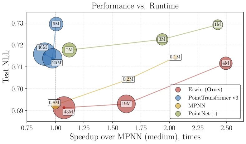
Figure 7: Test negative log-likelihood (NLL) of the predicted acceleration distribution for the molecular dynamics task (averaged over 3 runs). The baseline MPNN is taken from (Fu et al., 2022). The size of the markers reflects the number of parameters.

Molecular dynamics (MD) is essential for understanding physical and biological systems at the atomic level but remains computationally expensive even with neural network potentials due to all-atom force calculations and femtosecond timesteps required to maintain stability and accuracy. Fu et al. (2022) suggested accelerating MD simulation through coarse-grained dynamics with MPNN. In this experiment, we take a different approach and instead operate on the original representation but improve the runtime by employing our hardware-efficient model. Therefore, the question we ask is how much we can accelerate a simulation w.r.t. an MPNN without compromising the performance.

Dataset

The dataset consists of single-chain coarse-grained polymers (Webb et al., 2020; Fu et al., 2022) simulated using MD. Each system includes 4 types of coarse-grained beads interacting through bond, angle, dihedral, and non-bonded potentials. The training set consists of polymers with the repeated pattern of the beads while the polymers in the test set are constructed by randomly sampling sequences of the beads thus introducing a challenging distribution shift. The training set contains $100$ short trajectories ($50k$ $\tau$), while the test set contains $40$ trajectories that are $100$ times longer. Each polymer chain contains approximately $890$ beads on average.

Task

We follow the experimental setup from Fu et al. (2022). The model takes as input a polymer chain of $N$ coarse-grained beads. Each bead has a specific weight and is associated with the history $\{\dot{\mathbf{x}}_{t-16\Delta t},...,\dot{\mathbf{x}}_{t-\Delta t}\}$ of (normalized) velocities from $16$ previous timesteps at intervals of $\Delta t=5\tau$. The model predicts the mean $\mathbf{\mu}_{t}\in\mathbb{R}^{N\times 3}$ and variance $\mathbf{\sigma}_{t}^{2}\in\mathbb{R}_{+}^{N\times 3}$ of (normalized) acceleration for each bead, assuming a normal distribution. We train using negative log-likelihood loss

$$\mathcal{L}=-\log\mathcal{N}(\hat{\ddot{\mathbf{x}}}_{t}|\mathbf{\mu}_{t},\mathbf{\sigma}_{t}^{2})\vskip-2.0pt$$

between predicted and ground truth accelerations computed from the ground truth trajectories.

Table 1: Ablation on the cosmology task. Increasing window size improves performance at the cost of slower runtime (Erwin-S).

Ball Size	256	128	64	32
Test Loss	$\mathbf{0.595}$	$0.603$	$0.612$	$0.620$
Runtime, ms	$229.6$	$165.2$	$135.3$	$\mathbf{126.0}$

Table 2: Ablation study (MD task, Erwin-S) on the architectural choices: using MPNN in embedding, RPE (see Eq. 9) and cross-ball connection via rotating trees. Runtime includes building trees.

	Test Loss	Runtime, ms
w/o	$0.738$	$25.15$
$+$ MPNN	$0.720$	$26.07$
$+$ RPE	$0.715$	$26.05$
$+$ rotating tree	$0.712$	$26.73$

Results

The results are given in Fig. 7. As baselines, we use MPNN (Gilmer et al., 2017) as well as two hardware-efficient architectures: PointNet++ (Qi et al., 2017) and PointTransformer v3 (Wu et al., 2024). Notably, model choice has minimal impact on performance, potentially due to the absence of long-range interactions as the CG beads do not carry any charge. Furthermore, it is sufficient to only learn local bonded interactions. There is, however, a considerable improvement in runtime for Erwin ($1.7-2.5$ times depending on the size), which is only matched by smaller MPNN or PointNet++, both having significantly higher test loss.

5.3 Turbulent fluid dynamics

In the last experiment, we demonstrate the expressivity of our model by simulating turbulent fluid dynamics. The problem is notoriously challenging due to multiple factors: the inherently nonlinear behaviour of fluids, the multiscale and chaotic nature of turbulence, and the presence of long-range dependencies. Moreover, the geometry of the simulation domain and the presence of objects introduce complex boundary conditions thus adding another layer of complexity.

Dataset

We use EAGLE (Janny et al., 2023), a large-scale benchmark of unsteady fluid dynamics. Each simulation includes a flow source (drone) that moves in 2D environments with different boundary geometries producing airflow. The time evolution of velocity and pressure fields is recorded along with dynamically adapting meshes. The dataset contains $600$ different geometries of $3$ types, with approximately $1.1$ million 2D meshes averaging $3388$ nodes each. The total dataset includes $1184$ simulations with $990$ time steps per simulation. The dataset is split with 80% for training and 10% each for validation and testing.

Task

We follow the original experimental setup of the benchmark. The input is the velocity $V\in\mathbb{R}^{N\times 2}$ and pressure $P\in\mathbb{R}^{N\times 2}$ fields evaluated at every node of the mesh in the time step $t$ along with the type of the node. The task is to predict the state of the system at the next time step $t+1$. The training is done by predicting a trajectory of states of length $5$ and optimizing the loss

$$\mathcal{L}=\sum_{i=1}^{5}\left(\text{MSE}(V_{t+i},\hat{V}_{t+i})+\alpha\;\text{MSE}(P_{t+i},\hat{P}_{t+i})\right),$$

where $\alpha=0.1$ is the parameter that balances the importance of the pressure field over the velocity field.

Results

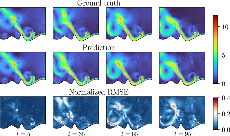
Figure 8: The norm of the velocity field at different steps of the rollout trajectories.

For comparison, we include the baselines from the original benchmark: MeshGraphNet (MGN; Pfaff et al., 2021), GAT (Velickovic et al., 2018), DilResNet (DRN; Stachenfeld et al., 2021) and EAGLE (Janny et al., 2023). The first two baselines are based on message-passing, while DilResNet operates on regular grids hence employing interpolation for non-uniform meshes. EAGLE uses message-passing to pool the mesh to a coarser representation with a fixed number of clusters, on which attention is then computed. The quantitative results are given in Table 3 and unrolling trajectories are shown in Fig. 8 and in Appendix B. Erwin demonstrates strong results on the benchmark and outperforms every baseline, performing especially well at predicting pressure. In terms of inference time and memory consumption, Erwin achieves substantial gains over EAGLE, being $3$ times faster and using $8$ times less memory.

Table 3: RMSE on velocity V and pressure P fields across different prediction horizons (mean $\pm$ std over 5 runs). Inference runtime and memory use computed for a batch of $8$, $3500$ nodes on average.

Horizon	$+1$		$+50$		Time	Mem.
Field / Unit	V	P	V	P	(ms)	(GB)
MGN	$0.081$	$0.43$	$0.592$	$2.25$	$40$	$0.7$
GAT	$0.170$	$64.6$	$0.855$	$163$	$44$	$0.5$
DRN	$0.251$	$1.45$	$0.537$	$2.46$	$42$	$\mathbf{0.2}$
EAGLE	$0.053$	$0.46$	$0.349$	$1.44$	$30$	$1.5$
Erwin	$\mathbf{0.044}$	$\mathbf{0.31}$	$\mathbf{0.281}$	$\mathbf{1.15}$	$\mathbf{11}$	$\mathbf{0.2}$
(Ours)	$\pm 0.001$	$\pm 0.01$	$\pm 0.001$	$\pm 0.06$

5.4 Ablation study

We also conducted an ablation study to examine the effect of increasing ball sizes on the model’s performance in the cosmology experiment, see Table 1. Given the presence of long-range interactions in the data, larger window sizes (and thus receptive fields) improve model performance, albeit at the cost of increased computational runtime. Our architectural ablation study on the MD task (Table 2) reveals that using MPNN at the embedding step produces substantial improvements, likely due to its effectiveness in learning local interactions.

6 Conclusion

We present Erwin, a hierarchical transformer that uses ball tree partitioning to process large-scale physical systems with linear complexity. Erwin achieves state-of-the-art performance on both the cosmology benchmark (Balla et al., 2024) and the EAGLE dataset (Janny et al., 2023), demonstrating its effectiveness across diverse physical domains. The efficiency of Erwin makes it a suitable candidate for any tasks that require modeling large particle systems, such as tasks in computational chemistry (Fu et al., 2024) or diffusion-based molecular dynamics (Jing et al., 2024).

Limitations and Future Work

Because Erwin relies on perfect binary trees, we need to pad the input set with virtual nodes, which induces computational overhead for ball attention computed over non-coarsened trees (first ErwinBlock). This issue can be circumvented by employing learnable pooling to the next level of the ball tree, which is always full, ensuring the remaining tree is perfect. Whether we can perform such pooling without sacrificing expressivity is a question that we leave to future research.

Erwin was developed by jointly optimizing for expressivity and runtime. As a result, certain architectural decisions are not optimal with respect to memory usage. In particular, we use a distance-based attention bias (see Eq. 10), for which both computational and memory requirements grow quadratically with the ball size. Developing alternative ways of introducing geometric information into attention computation could reduce these requirements. Finally, Erwin is neither permutation nor rotation equivariant, although rotation equivariance can be incorporated without compromising scalability. One possible approach is to use geometric algebra transformers (Brehmer et al., 2023) and omit the proposed cross-ball connections, as they rely on invariance-breaking tree building.

Appendix A Implementation details

Algorithm 1 BuildBallTree

 input Array of data points $D$ in $\mathbb{R}^{d}$

 output Ball tree node $B$

 

 if $|D|=1$ then

  Create leaf node $B$ containing single point in $D$

  return $B$

 end if

 

 # Find dimension of greatest spread

 $\delta\leftarrow\text{argmax}_{i\in{1,\ldots,d}}(\max_{x\in D}x_{i}-\min_{x\in D}x_{i})$

 

 # Find the median point along $\delta$

 $p\leftarrow\text{median}\{x_{\delta}\mid x\in D\}$ # Points left of median along $\delta$

 $L\leftarrow\{x\in D\mid x_{\delta}\leq p_{\delta}\}$ # Points right of median along $\delta$

 $R\leftarrow\{x\in D\mid x_{\delta}>p_{\delta}\}$

 

 # Recursively construct children

 $B.\text{child}_{1}\leftarrow\textsc{BuildBallTree}(L)$

 $B.\text{child}_{2}\leftarrow\textsc{BuildBallTree}(R)$

 

 return $B$

Ball tree construction

The algorithm used for constructing ball trees (Pedregosa et al., 2012) can be found in Alg. 1. Note that this implementation is not rotationally equivariant as it relies on choosing the dimension of the greatest spread which in turn depends on the original orientation. Examples of ball trees built in our experiments are shown in Fig. 9.

MPNN in the embedding

Erwin employs a small-scale MPNN in the embedding. More precisely, given a graph $G=(V,E)$ with nodes $v_{i}\in V$ and edges $e_{ij}\in E$, we compute multiple layers of message-passing as proposed in (Gilmer et al., 2017):

$$\mathbf{m}_{ij}=\text{MLP}_{e}(\mathbf{h}_{i},\mathbf{h}_{j},\mathbf{p}_{i}-\mathbf{p}_{j}),\qquad \mathrm{message}$$

$$\mathbf{m}_{i}\,\,\,=\sum_{j\in\mathcal{N}(i)}\mathbf{m}_{ij},\qquad \mathrm{aggregate}$$ (14)

$$\mathbf{h}_{i}=\text{MLP}_{h}(\mathbf{h}_{i},\mathbf{m}_{i}),\qquad \mathrm{update}$$

where $\mathbf{h}_{i}\in\mathbb{R}^{H}$ is a feature vector of $v_{i}$, $\mathcal{N}(i)$ denotes the neighborhood of $v_{i}$. The motivation for using an MPNN is to incorporate local neighborhood information into the model. Theoretically, attention should be able to capture it as well; however, this might require substantially increasing feature dimension and the number of attention heads, which would be prohibitively expensive for a large number of nodes in the original level of a ball tree.

In our experiments, we consistently maintain the size of MLP_e and MLP_h small ($H\leq 32$) such that embedding accounts for less than $5$% of total runtime.

Appendix B Extended experiments

B.1 Turbulent fluid dynamics

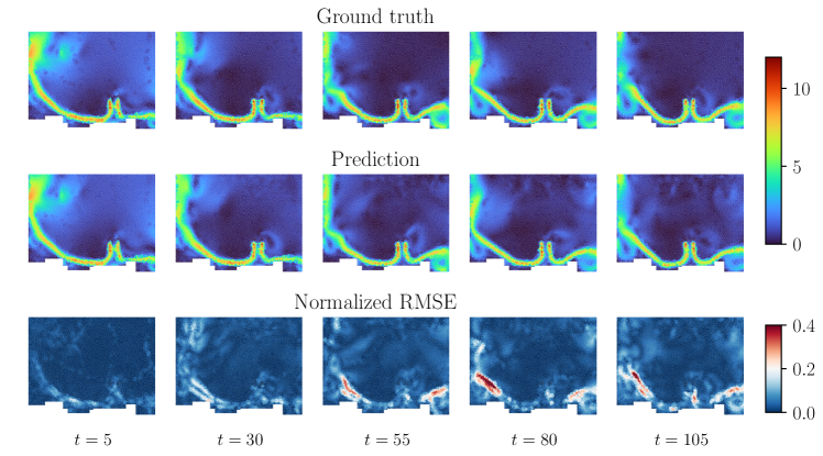
Figure 10: The norm of the velocity field at different steps of the rollout trajectories, predicted by Erwin.

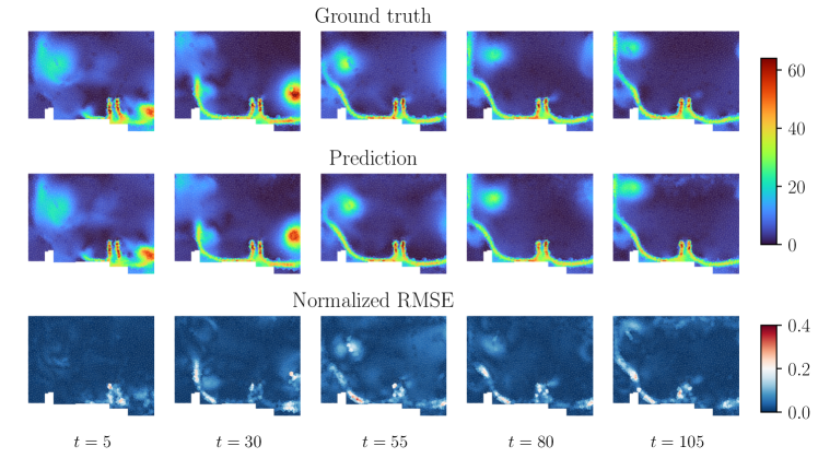
Figure 11: The norm of the pressure field at different steps of the rollout trajectories, predicted by Erwin.

We provide additional exemplary rollouts of Erwin for both velocity (Fig. 10) and pressure (Fig. 11) fields.

B.2 Airflow pressure modeling

Dataset

We use the ShapeNet-Car dataset generated by Umetani & Bickel (2018) and preprocessed by Alkin et al. (2024a). It consists of $889$ car models, each car being represented by $3586$ surface points in $3$D space. Airflow was simulated around each car for $10$s (Reynolds number $Re=5\times 10^{6}$) and averaged over the last $4$s to obtain pressure values at each point. The dataset is randomly split into $700$ training and $189$ test samples.

Task

Given surface points, the task is to predict the value of pressure $P\in\mathbb{R}^{N\times 1}$ at each point in $X^{N\times 3}$. The training is done by optimizing the mean squared error loss between predicted and ground truth pressures.

Table 4: Test MSE for ShapeNet-Car pressure prediction. [U] and [R] indicate U-Net- and ResNet-like structures respectively.

Model	MSE, $\times 10^{-2}$
U-Net	$6.13$
FNO	$4.04$
GINO	$2.34$
UPT	$2.31$
PointTransformer v3 [U]	$1.78$
Erwin (Ours) [U]	$1.42$
PointTransformer v3 [R]	$\mathbf{0.92}$
Erwin (Ours) [R]	$\mathbf{0.92}$

Results

The results are given in Table 4. We evaluate PointTransformer v3 and use the baseline results obtained by Alkin et al. (2024a) for U-Net (Ronneberger et al., 2015), FNO (Li et al., 2021), GINO (Li et al., 2023), and UPT (Alkin et al., 2024a). Both Erwin and PointTransformer v3 achieve significantly lower test MSE compared to other models, which can be attributed to their ability to capture fine geometric details by operating directly on the original point cloud. In comparison, other approaches introduce information loss through compression - UPT encodes the mesh into a latent space representation, while the remaining baselines interpolate the geometry onto regular grids and back. Moreover, in our experiments, ResNet-like configurations that did not include any coarsening performed dramatically better than the ones following the U-Net structure. Overall, this result highlights the potential for Erwin to be used as a scalable neural operator (Wang et al., 2024).

Figure 9: Examples of ball trees built on top of data. Partitions at different levels of ball trees are shown. Top: a polypeptide from the molecular dynamics task. Center: a domain from the EAGLE dataset. Bottom: a car surface from the ShapeNet-Car dataset.

Appendix C Experimental details

In this section, we provide experimental details regarding hyperparameter choice and optimization. All experiments were conducted on a single NVIDIA RTX A6000. All models were trained using the AdamW optimizer (Loshchilov & Hutter, 2019) with weight decay $0.01$ and a cosine decay schedule. The learning rate was tuned in the range $10^{-4}$ to $10^{-3}$ to minimize loss on the respective validation sets.

Cosmological simulations

We follow the experimental setup of the benchmark. The training was done for $5000$ epochs with batch size $16$ for point transformers and batch size $8$ for message-passing-based models. The implementation of SEGNN, NequIP and MPNN was done in JAX and taken from the original benchmark repository (Balla et al., 2024). We maintained the hyperparameters of the baselines used in the benchmark. For Erwin and PointTransformer, those are provided in Table 5. In Erwin’s embedding, we conditioned messages on Bessel basis functions rather than the relative position, which significantly improved overall performance.

Molecular dynamics

All models were trained with batch size $32$ for $50000$ training iterations with an initial learning rate of $5\cdot 10^{-4}$. We finetuned the hyperparameters of every model on the validation dataset (reported in Table 7).

Turbulent fluid dynamics

Baseline results are taken from (Janny et al., 2023), except for runtime and peak memory usage, which we measured ourselves. Erwin was trained with batch size $12$ for $4000$ epochs.

Airflow pressure modeling

We take the results of baseline models from Alkin et al. (2024a). Both Erwin and PointTransformer v3 were trained with batch size $32$ for $1000$ epochs, and their hyperparameters are given in Table 6).

Table 5: Model architectures for the cosmological simulations task. For varying sizes of Erwin, the values are given as (S/M).

Model	Parameter	Value
Point	Grid size	0.01
Transformer v3	Enc. depths	(2, 2, 6, 2)
	Enc. channels	(32, 64, 128, 256)
	Enc. heads	(2, 4, 8, 16)
	Enc. patch size	64
	Dec. depths	(2, 2, 2)
	Dec. channels	(64, 64, 128)
	Dec. heads	(2, 4, 8)
	Dec. patch size	64
	Pooling	(2, 2, 2)
Erwin	MPNN dim.	32
	Channels	32-512/64-1024
	Window size	64
	Enc. heads	(2, 4, 8, 16)
	Enc. depths	(2, 2, 6, 2)
	Dec. heads	(2, 4, 8)
	Dec. depths	(2, 2, 2)
	Pooling	(2, 2, 2, 1)

Table 6: Model architectures for the airflow pressure task.

Model	Parameter	Value
Point	Grid size	0.01
Transformer v3	Enc. depths	(2, 2, 2, 2, 2)
	Enc. channels	24-384
	Enc. heads	(2, 4, 8, 16, 32)
	Enc. patch size	256
	Dec. depths	(2, 2, 2, 2)
	Dec. channels	48-192
	Dec. heads	(4, 4, 8, 16)
	Dec. patch size	256
Erwin	MPNN dim.	8
	Channels	96
	Window size	256
	Enc. heads	(8, 16)
	Enc. depths	(6, 2)
	Dec. heads	(8,)
	Dec. depths	(2,)
	Pooling	(2, 1)
	MP steps	1

Table 7: Model architectures for the molecular dynamics task. For models of varying sizes, the values are given as (S/M/L).

Model	Parameter	Value
MPNN	Hidden dim.	48/64/128
	MP steps	6
	MLP layers	2
	Message agg-n	mean
PointNet++	Hidden dim.	64/128/196
	MLP layers	2
Point	Grid size	0.025
Transformer v3	Enc. depths	(2, 2, 2, 6, 2)
	Enc. channels	16-192/24-384/64-1024
	Enc. heads	(2, 4, 8, 16, 32)
	Enc. patch size	128
	Dec. depths	(2, 2, 2, 2)
	Dec. channels	16-96/48-192/64-512
	Dec. heads	(4, 4, 8, 16)
	Dec. patch size	128
Erwin	MPNN dim.	16/16/32
	Channels	(16-256/32-512/64-1024)
	Window size	128
	Enc. heads	(2, 4, 8, 16, 32)
	Enc. depths	(2, 2, 2, 6, 2)
	Dec. heads	(4, 4, 8, 16)
	Dec. depths	(2, 2, 2, 2)
	Pooling	(2, 2, 2, 2, 1)

References

- Alkin et al. (2024a) Alkin, B., Fürst, A., Schmid, S., Gruber, L., Holzleitner, M., and Brandstetter, J. Universal physics transformers: A framework for efficiently scaling neural operators. In Conference on Neural Information Processing Systems (NeurIPS), 2024a.
- Alkin et al. (2024b) Alkin, B., Kronlachner, T., Papa, S., Pirker, S., Lichtenegger, T., and Brandstetter, J. Neuraldem – real-time simulation of industrial particulate flows. arXiv preprint arXiv:2411.09678, 2024b.
- Arts et al. (2023) Arts, M., Satorras, V., Huang, C.-W., Zuegner, D., Federici, M., Clementi, C., Noé, F., Pinsler, R., and Berg, R. Two for one: Diffusion models and force fields for coarse-grained molecular dynamics. Journal of chemical theory and computation, 19, 09 2023. doi: 10.1021/acs.jctc.3c00702.
- Balla et al. (2024) Balla, J., Mishra-Sharma, S., Cuesta-Lázaro, C., Jaakkola, T. S., and Smidt, T. E. A cosmic-scale benchmark for symmetry-preserving data processing. arXiv preprint arXiv:2410.20516, 2024.
- Barnes & Hut (1986) Barnes, J. and Hut, P. A hierarchical O(N log N) force-calculation algorithm. Nature, 324(6096):446–449, 1986. doi: 10.1038/324446a0.
- Batzner et al. (2021) Batzner, S. L., Musaelian, A., Sun, L., Geiger, M., Mailoa, J. P., Kornbluth, M., Molinari, N., Smidt, T. E., and Kozinsky, B. E(3)-equivariant graph neural networks for data-efficient and accurate interatomic potentials. Nature Communications, 13, 2021.
- Bodnar et al. (2024) Bodnar, C., Bruinsma, W. P., Lucic, A., Stanley, M., Brandstetter, J., Garvan, P., Riechert, M., Weyn, J., Dong, H., Vaughan, A., Gupta, J. K., Tambiratnam, K., Archibald, A., Heider, E., Welling, M., Turner, R. E., and Perdikaris, P. Aurora: A foundation model of the atmosphere. arXiv preprint arXiv:2405.13063, 2024.
- Brandstetter et al. (2022) Brandstetter, J., Hesselink, R., van der Pol, E., Bekkers, E. J., and Welling, M. Geometric and physical quantities improve E(3) equivariant message passing. In International Conference on Learning Representations (ICLR), 2022.
- Brehmer et al. (2023) Brehmer, J., de Haan, P., Behrends, S., and Cohen, T. S. Geometric algebra transformer. In Conference on Neural Information Processing Systems (NeurIPS), 2023.
- Carrier et al. (1988) Carrier, J., Greengard, L., and Rokhlin, V. A fast adaptive multipole algorithm for particle simulations. SIAM Journal on Scientific and Statistical Computing, 9(4):669–686, 1988. doi: 10.1137/0909044.
- Cohen & Welling (2016) Cohen, T. and Welling, M. Group equivariant convolutional networks. In International Conference on Machine Learning (ICML), 2016.
- Dao (2024) Dao, T. Flashattention-2: Faster attention with better parallelism and work partitioning. In International Conference on Learning Representations (ICLR), 2024.
- Fu et al. (2022) Fu, X., Xie, T., Rebello, N. J., Olsen, B. D., and Jaakkola, T. Simulate time-integrated coarse-grained molecular dynamics with multi-scale graph networks. Trans. Mach. Learn. Res., 2023, 2022.
- Fu et al. (2024) Fu, X., Xie, T., Rosen, A. S., Jaakkola, T. S., and Smith, J. Mofdiff: Coarse-grained diffusion for metal-organic framework design. In International Conference on Learning Representations (ICLR), 2024.
- Gilmer et al. (2017) Gilmer, J., Schoenholz, S. S., Riley, P. F., Vinyals, O., and Dahl, G. E. Neural message passing for quantum chemistry. In International Conference on Machine Learning (ICML), 2017.
- Hockney & Eastwood (2021) Hockney, R. and Eastwood, J. Computer Simulation Using Particles. CRC Press, 2021. ISBN 9781439822050. URL https://books.google.nl/books?id=nTOFkmnCQuIC.
- Janny et al. (2023) Janny, S., Béneteau, A., Nadri, M., Digne, J., Thome, N., and Wolf, C. EAGLE: large-scale learning of turbulent fluid dynamics with mesh transformers. In International Conference on Learning Representations (ICLR), 2023.
- Jing et al. (2024) Jing, B., Stärk, H., Jaakkola, T. S., and Berger, B. Generative modeling of molecular dynamics trajectories. arXiv preprint arXiv:2409.17808, 2024.
- Kang et al. (2023) Kang, Y., Tran, G., and Sterck, H. D. Fast multipole attention: A divide-and-conquer attention mechanism for long sequences. arXiv preprint arXiv:2310.11960, 2023.
- Kovács et al. (2023) Kovács, D. P., Moore, J. H., Browning, N. J., Batatia, I., Horton, J. T., Kapil, V., Witt, W. C., Magdău, I.-B., Cole, D. J., and Csányi, G. Mace-off23: Transferable machine learning force fields for organic molecules, 2023.
- Li et al. (2021) Li, Z., Kovachki, N. B., Azizzadenesheli, K., Liu, B., Bhattacharya, K., Stuart, A. M., and Anandkumar, A. Fourier neural operator for parametric partial differential equations. In International Conference on Learning Representations (ICLR), 2021.
- Li et al. (2023) Li, Z., Kovachki, N. B., Choy, C. B., Li, B., Kossaifi, J., Otta, S. P., Nabian, M. A., Stadler, M., Hundt, C., Azizzadenesheli, K., and Anandkumar, A. Geometry-informed neural operator for large-scale 3d pdes. In Conference on Neural Information Processing Systems (NeurIPS), 2023.
- Liu et al. (2021) Liu, Z., Lin, Y., Cao, Y., Hu, H., Wei, Y., Zhang, Z., Lin, S., and Guo, B. Swin transformer: Hierarchical vision transformer using shifted windows. In International Conference on Computer Vision (ICCV), 2021.
- Liu et al. (2023) Liu, Z., Yang, X., Tang, H., Yang, S., and Han, S. Flatformer: Flattened window attention for efficient point cloud transformer. In Conference on Computer Vision and Pattern Recognition(CVPR), 2023.
- Loshchilov & Hutter (2019) Loshchilov, I. and Hutter, F. Decoupled weight decay regularization. In International Conference on Learning Representations (ICLR), 2019.
- Majumdar et al. (2020) Majumdar, S., Sun, J., Golding, B., Joe, P., Dudhia, J., Caumont, O., Gouda, K. C., Steinle, P., Vincendon, B., Wang, J., and Yussouf, N. Multiscale forecasting of high-impact weather: Current status and future challenges. Bulletin of the American Meteorological Society, 102:1–65, 10 2020. doi: 10.1175/BAMS-D-20-0111.1.
- Pedregosa et al. (2012) Pedregosa, F., Varoquaux, G., Gramfort, A., Michel, V., Thirion, B., Grisel, O., Blondel, M., Prettenhofer, P., Weiss, R., Dubourg, V., VanderPlas, J., Passos, A., Cournapeau, D., Brucher, M., Perrot, M., and Duchesnay, E. Scikit-learn: Machine learning in python. arXiv preprint arXiv:1201.0490, 2012.
- Pfaff et al. (2021) Pfaff, T., Fortunato, M., Sanchez-Gonzalez, A., and Battaglia, P. W. Learning mesh-based simulation with graph networks. In International Conference on Learning Representations (ICLR), 2021.
- Pfalzner & Gibbon (1996) Pfalzner, S. and Gibbon, P. Many-Body Tree Methods in Physics. Cambridge University Press, 1996.
- Qi et al. (2017) Qi, C. R., Yi, L., Su, H., and Guibas, L. J. Pointnet++: Deep hierarchical feature learning on point sets in a metric space. In Conference on Neural Information Processing Systems (NeurIPS), 2017.
- Rogozhnikov (2022) Rogozhnikov, A. Einops: Clear and reliable tensor manipulations with einstein-like notation. In International Conference on Learning Representations (ICLR), 2022.
- Ronneberger et al. (2015) Ronneberger, O., Fischer, P., and Brox, T. U-net: Convolutional networks for biomedical image segmentation. In International Conference on Medical Image Computing and Computer-Assisted Intervention (MICCAI), 2015.
- Shazeer (2020) Shazeer, N. GLU variants improve transformer. arXiv preprint arXiv:2002.05202, 2020.
- Stachenfeld et al. (2021) Stachenfeld, K. L., Fielding, D. B., Kochkov, D., Cranmer, M. D., Pfaff, T., Godwin, J., Cui, C., Ho, S., Battaglia, P. W., and Sanchez-Gonzalez, A. Learned coarse models for efficient turbulence simulation. arXiv preprint arXiv:2112.15275, 2021.
- Sun et al. (2022) Sun, P., Tan, M., Wang, W., Liu, C., Xia, F., Leng, Z., and Anguelov, D. Swformer: Sparse window transformer for 3d object detection in point clouds. In European Conference on Computer Vision (ECCV), 2022.
- Umetani & Bickel (2018) Umetani, N. and Bickel, B. Learning three-dimensional flow for interactive aerodynamic design. ACM Trans. Graph., 37(4):89, 2018. URL https://doi.org/10.1145/3197517.3201325.
- Vaswani et al. (2017) Vaswani, A., Shazeer, N., Parmar, N., Uszkoreit, J., Jones, L., Gomez, A. N., Kaiser, L., and Polosukhin, I. Attention is all you need. In Conference on Neural Information Processing Systems (NeurIPS), pp. 5998–6008, 2017.
- Velickovic et al. (2018) Velickovic, P., Cucurull, G., Casanova, A., Romero, A., Liò, P., and Bengio, Y. Graph attention networks. In International Conference on Learning Representations (ICLR), 2018.
- Wang (2023) Wang, P.-S. Octformer: Octree-based transformers for 3D point clouds. ACM Transactions on Graphics (SIGGRAPH), 42(4), 2023.
- Wang et al. (2024) Wang, S., Seidman, J. H., Sankaran, S., Wang, H., Pappas, G. J., and Perdikaris, P. Bridging operator learning and conditioned neural fields: A unifying perspective. arXiv preprint arXiv:2405.13998, 2024.
- Watson et al. (2023) Watson, J. L., Juergens, D., Bennett, N. R., Trippe, B. L., Yim, J., Eisenach, H. E., Ahern, W., Borst, A. J., Ragotte, R. J., Milles, L. F., Wicky, B. I. M., Hanikel, N., Pellock, S. J., Courbet, A., Sheffler, W., Wang, J., Venkatesh, P., Sappington, I., Torres, S. V., Lauko, A., Bortoli, V. D., Mathieu, E., Ovchinnikov, S., Barzilay, R., Jaakkola, T., DiMaio, F., Baek, M., and Baker, D. De novo design of protein structure and function with rfdiffusion. Nature, 620:1089 – 1100, 2023.
- Webb et al. (2020) Webb, M., Jackson, N., Gil, P., and de Pablo, J. Targeted sequence design within the coarse-grained polymer genome. Science Advances, 6:eabc6216, 10 2020. doi: 10.1126/sciadv.abc6216.
- Wessels et al. (2024) Wessels, D. R., Knigge, D. M., Papa, S., Valperga, R., Vadgama, S. P., Gavves, E., and Bekkers, E. J. Grounding continuous representations in geometry: Equivariant neural fields. arXiv preprint arXiv:2406.05753, 2024.
- Wu et al. (2024) Wu, X., Jiang, L., Wang, P., Liu, Z., Liu, X., Qiao, Y., Ouyang, W., He, T., and Zhao, H. Point transformer V3: simpler, faster, stronger. In Conference on Computer Vision and Pattern Recognition(CVPR), 2024.
- Zhu & Soricut (2021) Zhu, Z. and Soricut, R. H-transformer-1d: Fast one-dimensional hierarchical attention for sequences. In Conference on Neural Information Processing Systems (NeurIPS), pp. 3801–3815. Association for Computational Linguistics, 2021.