Latency-Aware Resource Allocation for Integrated Communications, Computation, and Sensing in Cell-Free mMIMO Systems

Abstract

In this paper, we investigate a cell-free massive multiple-input and multiple-output (MIMO)-enabled integration communication, computation, and sensing (ICCS) system, aiming to minimize the maximum computation latency to guarantee the stringent sensing requirements. We consider a two-tier offloading framework, where each multi-antenna terminal can optionally offload its local tasks to either multiple mobile-edge servers for distributed computation or the cloud server for centralized computation while satisfying the sensing requirements and power constraint. The above offloading problem is formulated as a mixed-integer programming and non-convex problem, which can be decomposed into three sub-problems, namely, distributed offloading decision, beamforming design, and execution scheduling mechanism. First, the continuous relaxation and penalty-based techniques are applied to tackle the distributed offloading strategy. Then, the weighted minimum mean square error (WMMSE) and successive convex approximation (SCA)-based lower bound are utilized to design the integrated communication and sensing (ISAC) beamforming. Finally, the other resources can be judiciously scheduled to minimize the maximum latency. A rigorous convergence analysis and numerical results substantiate the effectiveness of our method. Furthermore, simulation results demonstrate that multi-point cooperation in cell-free massive MIMO-enabled ICCS significantly reduces overall computation latency, in comparison to the benchmark schemes.

I Introduction

Recently, integrated communication and sensing (ISAC) has emerged as one of the potential paradigms for the sixth generation (6G) wireless communication systems [1, 2, 3]. ISAC is able to simultaneously achieve high-accuracy sensing and high-quality wireless connectivity, leveraging the similarities in hardware and signal processing. Compared to the legacy wireless networks, the ISAC-enabled systems can significantly improve spectrum efficiency, reduce infrastructure costs, and offer flexible and versatile solutions for a wide range of applications, such as autonomous driving [4, 5] and smart manufacturing [6].

The integration of ISAC with massive multiple-input multiple-output (MIMO) techniques offers significantly spatial beamforming gains, enhancing both communication and sensing capabilities [7, 8], and thus MIMO-ISAC has extracted extensive research attentions from academia and industry [9, 10, 11, 12, 13, 14, 15, 16]. For example, by optimizing the ISAC beamforming, the Cramér-Rao bound (CRB) for sensing is derived in [9] while considering the minimal communication requirement. Since echo and communication signals share the same frequency and time resources, they can significantly interfere with each other, ultimately degrading both communication and sensing performance. To theoretically analyze this issue, the authors of [10] derive the CRB-rate region for a single target, revealing the trade-off bound between communication and sensing. Based on their results in [10], the fundamental trade-off between the achievable rate and the multi-target estimation CRB is analyzed in [11]. Considering the full-duplex operation for both radar and communication, the downlink precoding scheme and uplink transmission power are jointly devised to maximize the sum rate [12]. Then, to mitigate the severe inter-cell interference, the authors of [13] proposed an interference management, and the beamforming is devised by exploiting the multi-cell cooperation [14]. Considering the cell-free massive MIMO systems, the cooperative CRB-rate bound is studied in the cell-free massive MIMO systems [15]. Furthermore, to tackle the self-interference posed by ISAC, the authors of [16] assume that each AP can work as sensing or communication mode only, and devise the optimal operation mode of each AP by solving zero–one programming problem. Although the ISAC technique exhibits the tremendous advantages, how to enable real-time control according to the acquired sensing information remains elusive.

To address the above challenges, extensive contributions have been devoted to explore the seamless integration of communication, computation, and sensing (ICCS) technology in the MIMO systems [17, 18, 19, 20, 21]. Particularly, by using the superposition property of multiple access channels to aggregate massive data streams, the authors of [17] and [18] demonstrate that the over-the-air computation (AirComp) technique can significantly enhance the communication performance and computation error, respectively. By fully exploiting the potential of mobile edge computing (MEC), the communication and computation resources are judiciously optimized to minimize the energy consumption [19]. Then, considering the cloud computation (CC), the three-tier computation framework is investigated [20]. Furthermore, to minimize the CRB of radar sensing while guaranteeing users’ communication requirements, the semi-definite relaxation (SDR)-based alternating optimization and SDR-based successive convex approximation (SCA) algorithms are proposed in [21]. Although the existing research in [17, 18, 19, 20, 21] has revealed that the MIMO-enabled ICCS can significantly enhance system performance, it is still worth investigating how to implement ICCS in the cell-free massive MIMO systems and characterizing the benefits of cooperative communication and computation by using distributed APs or servers.

To date, existing results have demonstrated significant benefits through the integration of computation and communication in cell-free massive MIMO systems [22, 23, 24, 25]. For example, the advantage of distributed computation and cooperative communication is explored in [22]. Based on MEC and CC, the multi-tier offloading strategy is investigated to minimize computation latency with perfect fronthaul link [23]. To analyze the impact of limited fronthaul capacity on system performance, the balance between offloading decision and computation is studied in [24]. Then, to further reduce the burden of information exchange in the cell-free massive MIMO systems, the non-orthogonal transmissions is investigated in [25]. Whilst the aforementioned contributions have demonstrated the merits of task offloading and computation within a cell-free massive MIMO framework, the seamless integration of sensing alongside communication and computation remains an open research area, thereby prompting our exploration of the cell-free massive MIMO-enabled ICCS.

To the best of the authors’ knowledge, there is a paucity of work that has exploited the distributed computation offloading strategy in cell-free massive MIMO-enabled ICCS systems. To fully unleash the potential of distributed and centralized computations in cell-free massive MIMO systems, the offloading strategy, beamforming, and execution resources are jointly devised to minimize the maximum computation latency, while satisfying the sensing requirements, power constraints and computation capacity. The main contributions of this paper are summarized as follows:

1. By exploring the ICCS in the cell-free massive MIMO systems, we propose a two-tier offloading strategy for the efficient implementation to unlock the potential for distributed communication and computation. Relying on the MIMO beamforming technique, each multi-antenna terminal can optionally offload its task to multiple APs for mobile edge computation or cloud sever for cloud computation. In this paper, we aim to minimize the maximum latency by jointly optimizing the offloading strategy, beamforming, execution frequency, and other resources, which is formulated as a mix-integer programming and non-convex problem.

2. To tackle this problem, we decompose it into three sub-problems, namely, distributed offloading decision, beamforming design, and execution scheduling mechanism. Firstly, to address the mix-integer programming problem, we adopt the continuous relaxation and penalty techniques to obtain the solution of offloading strategy. Then, with the given offloading decision, the weighted minimum mean square error (WMMSE) method and a lower bound based on SCA method are applied to solve the non-convex problem. Finally, the execution frequency and other resources can be obtained by solving the convex problem. Furthermore, the convergence of proposed algorithm is mathematically proved.

3. By strategically allocating computational resources and designing communication beamforming, the maximum latency, including the computation and computation delays, can be significantly reduced, facilitating seamless control. Furthermore, while distributed offloading offers potential advantages over centralized approaches, inter-user communication interference remains a critical bottleneck, which is validated by our simulation results. More importantly, numerical result demonstrate that our proposed method is superior over other benchmarks, which verifies the effectiveness of our proposed method.

The remainder of the paper is organized as follows. The system model is provided and a general latency is given in Section II. The optimization algorithm is formulated and designed in Section III. In Section IV, extensive numerical results are presented. Finally, our conclusions are drawn in Section V.

II System Model

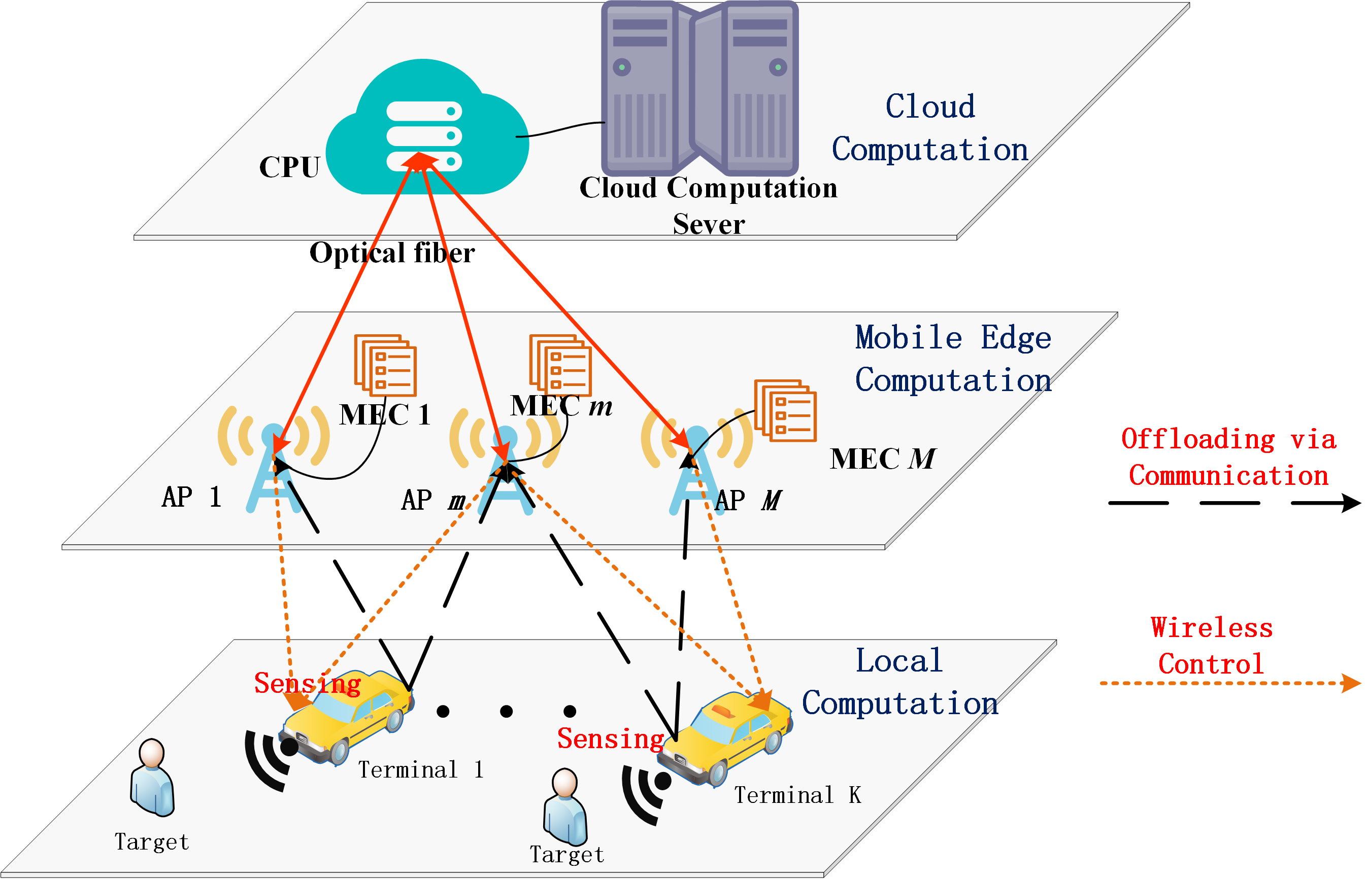
Figure 1: System model for ICCS in a cell-free mMIMO system.

As shown in Fig. 1, $M$ APs, each equipped with $N$ antennas, are linked with an edge server to provide MEC service for $K$ mobile vehicles, each equipped with $N_{t}$ transmission antennas and $N_{r}$ receiving antennas, respectively. Denoted the set of mobile vehicles and APs as $\mathcal{K}=\{1,\cdots,K\}$ and $\mathcal{M}=\{1,\cdots,M\}$, respectively. To enhance the system of scalability, we adopt the user-centric approach by defining $\mathcal{M}_{k}\in\mathcal{M}$ as the set of APs that provide communication and computation service for the $k$-th terminal. In particular, the $k$-th mobile vehicle can sense the environment, including the location, velocity, and acceleration, to construct the data set with $D_{k}$ bits, $\forall k\in\mathcal{K}$. Mobile vehicles process computational resources and execute operations, such as braking and slowing down, in response to the concurrent sensing data. However, owing to the limited processing capacity, power consumption, and strict latency constraints, mobile vehicles are generally unable to process a large amount of data by relying on local computation. To tackle this issue, the $k$-th mobile vehicle can offload some specific tasks to either nearby APs for distributed computation or the centralized processing unit (CPU) for centralized computation. For MEC, the $k$-th vehicle can divide $D_{k}$ bits into several parts, $D_{m,k}$ bits with $D_{k}=\sum\limits_{m\in\mathcal{M}_{k}}D_{m,k}$, and then transmit these tasks to several APs for distributed edge computation. Similarly, for CC, these tasks are first delivered to multiple APs, and then transmitted to the CPU for centralized cloud computation.

II-A Edge-to-AP Communication Model

The $k$-th mobile vehicle simultaneously transmits the signal $s_{k,m}$ for offloading task to the $m$-th AP and radar signal $s^{\text{sen}}_{k}$ for sensing, leading to the transmitted signal

$${\mathbf{x}}_{k}=\sum_{m\in\mathcal{M}_{k}}\mathbf{w}_{k,m}s_{k,m}+\mathbf{w}^{\text{sen}}_{k}\mathbf{s}^{\text{sen}}_{k},$$ (1)

where $\mathbf{w}_{k,m}\in{\mathbb{C}}^{N_{t}\times 1}$ is the precoding vector designed for the $m$-th AP, and $\mathbf{w}^{\text{sen}}_{k}\in\mathbb{C}^{N_{t}\times 1}$ represents the corresponding sensing beamforming. For ease of analysis but without loss of generality, we assume that the date symbol has unit power, i.e., $\mathbb{E}\{s_{k,m}s^{H}_{k,m}\}=1$. Furthermore, $s_{k,m}$ and $s^{\text{sen}}_{k}$ are assumed to be independent with each other.

The channel between the $k$-th vehicle and the $m$-th AP is defined as $\mathbf{H}_{k,m}\in\mathbb{C}^{N\times N_{t}}$, and the $[n,m]$-th element of $\mathbf{H}_{k,m}$ is given by

$$[\mathbf{H}_{k,m}]_{n,m}=\sqrt{\beta_{k,m}}h_{n,m},\forall n\in[1,\cdots,N],\forall m\in[1,\cdots,N_{t}],$$ (2)

where $\beta_{k,m}$ is the large-scale fading factor related to distance, and $h_{n,m}$ is the small-scale fading factor that follows a complex Gaussian distribution with zero mean and unit variance. Then, the received signal $\mathbf{y}_{k,m}\in{\mathbb{C}}^{N\times 1}$ at the $m$-th AP can be expressed as

$$\begin{split}\mathbf{y}_{k,m}&=\sum^{K}_{k^{\prime}=1}\mathbf{H}_{k^{\prime},m}\mathbf{x}_{k^{\prime}}+\mathbf{n}_{m},\\ &=\mathbf{H}_{k,m}\mathbf{w}_{k,m}s_{k,m}+\mathbf{H}_{k,m}\Big{(}\sum_{m^{\prime}\in\{\mathcal{M}_{k}\backslash m\}}\mathbf{w}_{k,m^{\prime}}s_{k,m^{\prime}}+\mathbf{w}^{\text{sen}}_{k}s^{\text{sen}}_{k}\Big{)}\\ &\quad+\sum^{K}_{k^{\prime}\neq k}{\sum_{m^{\prime}\in\mathcal{M}_{k^{\prime}}}\Big{(}\mathbf{H}_{k^{\prime},m}\mathbf{w}_{k^{\prime},m^{\prime}}s_{k^{\prime},m^{\prime}}+\mathbf{H}_{k^{\prime},m}\mathbf{w}^{\text{sen}}_{k^{\prime}}s^{\text{sen}}_{k^{\prime}}\Big{)}}+\mathbf{n}_{m},\end{split}$$ (3)

where $\mathbf{n}_{m}\sim\mathcal{CN}(0,\mathbf{I}_{N})$ represents the normalized additive white Gaussian noise (AWGN) at the $m$-th AP. Based on the received signal given in (3), the achievable data rate between the $k$-th vehicle and $m$-th AP can be expressed as [26]

$$R_{k,m}=B\log_{2}\det\Big{(}\mathbf{I}_{N}+\mathbf{H}_{k,m}\mathbf{w}_{k,m}\mathbf{w}^{H}_{k,m}\mathbf{H}^{H}_{k,m}{\mathbf{N}}^{-1}_{k,m}\Big{)},$$ (4)

where $B$ is the bandwidth, $\mathbf{N}_{k,m}$ is the overall interference and background noise, which can be expressed as

$$\begin{split}{\mathbf{N}}_{k,m}&=\sum_{m^{\prime}\in\{{{\cal M}_{k}}\backslash m\}}\mathbf{H}_{k,m}\mathbf{w}_{k,m^{\prime}}\mathbf{w}^{H}_{k,m^{\prime}}\mathbf{H}^{H}_{k,m}+\mathbf{H}_{k,m}\mathbf{w}_{k}^{\text{sen}}(\mathbf{w}^{\text{sen}}_{k})^{H}\mathbf{H}^{H}_{k,m}\\ &\quad+\sum^{K}_{k^{\prime}\neq k}{\sum_{m^{\prime}\in\mathcal{M}_{k^{\prime}}}\Big{(}\mathbf{H}_{k^{\prime},m}\mathbf{w}_{k^{\prime},m^{\prime}}\mathbf{w}^{H}_{k^{\prime},m^{\prime}}\mathbf{H}^{H}_{k^{\prime},m}+\mathbf{H}_{k^{\prime},m}\mathbf{w}^{\text{sen}}_{k^{\prime}}(\mathbf{w}^{\text{sen}}_{k^{\prime}})^{H}\mathbf{H}^{H}_{k^{\prime},m}\Big{)}}+\mathbf{I}_{N}.\end{split}$$ (5)

As can be seen from (5), inter-user interference escalates with an increasing number of offloading APs, leading to a decline in communication rates. Consequently, a trade-off exists between the number of offloading APs and the maximum latency.

II-B Edge-Node Sensing Model

Next, we model the target echo signal at the vehicles’ edge node , by assuming that the radar channel consists of line-of-sight (LoS) paths and both the transmit and receive uniform linear arrays (ULAs) at the vehicle are half-wavelength antenna spacing. Besides, the $k$-th vehicle can suppress the self-interference sufficiently via the corresponding techniques [19, 27]. The received echo signal is given by

$${\mathbf{y}}_{k}^{s}=\eta^{RT}_{k}\mathbf{a}_{r}(\theta_{k})\mathbf{a}_{t}^{H}(\theta_{k}){\mathbf{x}}_{k}+\sum^{K}_{k^{\prime}\neq k}{\mathbf{H}_{k,k^{\prime}}{\mathbf{x}}_{k^{\prime}}}+\mathbf{n}_{s},$$ (6)

where $\eta_{RT}$ contains the impacts of the path loss and complex reflection coefficients of the target and $\theta_{k}$ represents the angle of arrival related to the $k$-th vehicle’s sensing target [20]. $\mathbf{n}_{s}\sim\mathcal{CN}(0,\mathbf{I}_{N_{r}})$ denotes the normalized AWGN with zero mean and unit variance at the $k$-th vehicle, $\mathbf{a}_{r}(\theta)=[1,e^{-j2\pi\frac{d}{\lambda}\sin\theta},\cdots,e^{-j2\pi\frac{d}{\lambda}(N_{r}-1)\sin\theta}]^{T}$ denotes the receive steering vector, and $\mathbf{a}_{t}(\theta)=[1,e^{-j2\pi\frac{d}{\lambda}\sin\theta},\cdots,e^{-j2\pi\frac{d}{\lambda}(N_{t}-1)\sin\theta}]^{T}$ is transmitted array steering vector. $\mathbf{H}_{k,k^{\prime}}=\sqrt{\beta_{k,k^{\prime}}}\mathbf{\hat{H}}_{k,k^{\prime}}\in\mathbb{C}^{N_{r}\times N_{t}}$ denotes the interference channel from vehicle $k^{\prime}$ to vehicle $k$, $\beta_{k,k^{\prime}}$ is the large-scale fading factor related to distance, and $\mathbf{\hat{H}}_{k,k^{\prime}}$ is the small-scale fading factors, each element of which follows the complex Gaussian distribution with zero mean and unit variance. Besides, we assume that $\eta^{RT}_{k}$ and $\theta_{k}$ are known or previously coarse estimation at the vehicle for designing the best suitable transmit signal to detect this specific target of interest [20]. Then, based on (6), the $k$-th vehicle can capture the desired reflected signal of the point target, and thus the radar SINR can be written as

$$\begin{split}\text{SINR}_{k}^{\text{sen}}&=\frac{\mathbb{E}\{\left\|\eta^{RT}_{k}\mathbf{a}_{r}(\theta_{k})\mathbf{a}_{t}^{H}(\theta_{k}){\mathbf{x}}_{k}\right\|^{2}\}}{\mathbb{E}\{\|\mathbf{n}_{s}\|^{2}\}+\sum^{K}_{k^{\prime}\neq k}{\mathbb{E}\{\|\mathbf{H}_{k,k^{\prime}}{\mathbf{x}}_{k^{\prime}}\|^{2}\}}}\\ &=\frac{(\eta^{RT}_{k})^{2}\text{tr}\{\mathbf{a}_{r}(\theta)\mathbf{a}_{t}^{H}(\theta_{k})\mathbf{g}_{k}\mathbf{g}^{H}_{k}\mathbf{a}_{t}(\theta_{k})\mathbf{a}_{r}^{H}(\theta_{k})\}}{N_{r}+\sum^{K}_{k^{\prime}\neq k}{\text{tr}\{\mathbf{H}_{k,k^{\prime}}\mathbf{g}_{k}\mathbf{g}^{H}_{k}\mathbf{H}^{H}_{k,k^{\prime}}\}}},\end{split}$$ (7)

where $\text{tr}\{\bf X\}$ denotes the trace of matrix $\bf X$, $\mathbf{g}_{k}=\sum_{m\in\mathcal{M}_{k}}\mathbf{w}_{k,m}+\mathbf{w}^{\text{sen}}_{k}$ is sum of ISAC precoding vector from vehicle $k$.

II-C Computation Model

To characterize the computation strategy, i.e., local computation, mobile edge computation, and cloud computation, adopted by the $k$-th vehicle, $\forall k\in\{1,\cdots,K\}$, we define the offloading variables $\mathbf{b}_{k}=[b_{k,1},\cdots,b_{k,M}]^{T}$ with $b_{k,m}\in[0,1]$, $\forall m\in\{1,\cdots,M\}$ and $\mathbf{c}_{k}=[c_{k,1},\cdots,c_{k,M}]^{T}$ with $c_{k,m}\in[0,1]$, $\forall m\in\{1,\cdots,M\}$. When $b_{k,m}\neq 0$ and $c_{k,m}=0$, $\forall k,m$, the task is offloaded to the $m$-th edge server for computation. If $b_{k,m}=0$ and $c_{k,m}\neq 0$, $\forall k,m$, the task is executed by the cloud computation server. For $b_{k,m}=0$ and $c_{k,m}=0$, $\forall k,m$, the task is performed by local vehicle $k$. Based on this definition, we have

$$\sum^{M}_{m=1}(b_{k,m}+c_{k,m})\in\{0,1\}.$$ (8)

II-C1 Local Computation

For local computation, $D_{k}$ bits need to be computed locally. Therefore, the local computation latency is given by

$$T^{\text{Loc}}_{k}=\frac{\alpha^{\text{Loc}}_{k}D_{k}}{f^{\text{Loc}}_{k}},$$ (9)

where $\alpha^{\text{Loc}}_{k}$ and $f^{\text{Loc}}_{k}$ represent the local CPU cycle and CPU computing frequency of the vehicle $k$, respectively. Then, the total power consumption of local computation and transmission is

$$P_{k}^{\text{Loc}}=\kappa_{k}^{\text{Loc}}(f^{\text{Loc}}_{k})^{3}+\mathbf{g}^{H}_{k}\mathbf{g}_{k},$$ (10)

where $\kappa_{k}^{\text{Loc}}$ is a constant related to the hardware architecture of vehicle $k$.

II-C2 MEC

For MEC, the $k$-th vehicle transmits $D_{k}$ bits to the APs of set $\mathcal{M}_{k}$. The transmission latency from the vehicle $k$ to the $m$-th AP, $\forall m\in\mathcal{M}_{k}$, is given by

$$T_{k,m}^{\text{MECTR}}=\frac{b_{k,m}D_{k}}{R_{k,m}}.$$ (11)

Then, based on the received $D_{k}$ bits, the $m$-th mobile edge server linked with the $m$-th AP can compute its decision. The edge computation latency is given by

$$T^{\text{MECc}}_{k,m}=\frac{\alpha^{\text{MEC}}_{m}b_{k,m}D_{k}}{f^{\text{MEC}}_{k,m}},$$ (12)

where $\alpha^{\text{MEC}}_{m}$ and $f^{\text{MEC}}_{k,m}$ represent the CPU cycle and CPU computing frequency allocated to the $k$-th vehicle by AP $m$, respectively. Based on the above discussions, the latency for processing tasks allocated by vehicle $k$ to AP $m$ can be expressed as

$$T^{\text{MEC}}_{k}=\max\{T^{\text{MECTR}}_{k,m}+T^{\text{MECc}}_{k,m}\},\forall m\in\mathcal{M}.$$ (13)

Due to the limited computational capacity of the edge server, we have

$$\sum_{k\in\mathcal{K}}U(b_{k,m})f^{\text{MEC}}_{k,m}\leq F^{\text{MEC},\max}_{m},\forall m\in\mathcal{M},$$ (14)

where $U(t)$ is 1 when $t>0$ and $U(t)$ is 0 for $t\leq 0$. Then, the power consumption of the $m$-th edge server is given by

$$P^{\text{MEC}}_{m}=\sum_{k\in\mathcal{K}}{U(b_{k,m})\kappa_{m}^{\text{MEC}}(f^{\text{MEC}}_{k,m})^{3}},\forall m\in\mathcal{M},$$ (15)

where $\kappa_{m}^{\text{MEC}}$ is a constant related to the hardware architecture of the edge server $m$.

II-C3 CC

The latency of cloud computation can be divided into three parts, including transmission latency from the vehicle to multiple APs, transmission latency from all APs to the CPU, and computation latency for cloud computation. Firstly, the $k$-th vehicle can simultaneously transmit data to multiple APs of set $\mathcal{M}_{k}$, and the corresponding transmission latency is given by

$$T^{\text{V2ATra}}_{k,m}=\frac{c_{k,m}D_{k}}{R_{k,m}},\forall m\in\mathcal{M}_{k}.$$ (16)

Then, the received signal is delivered to the CPU linked to the cloud computation server. The transmission latency from the $m$-th AP to the CPU can be expressed as

$$T^{\text{A2CTra}}_{k,m}=\frac{c_{k,m}D_{k}}{r^{f}_{k,m}},\forall m\in\mathcal{M}_{k},$$ (17)

where $r^{f}_{k,m}$ is the transmission bandwidth between the $m$-th AP and the CPU via optical fiber. Based on the received signal, the latency of cloud computation is given by

$$T^{\text{CCom}}_{k,m}=\frac{\alpha^{\text{CC}}D_{k}}{f^{\text{CC}}_{k}},$$ (18)

where $\alpha^{\text{CC}}$ and $f^{\text{CC}}_{k}$ are the processing density and the allocated local computation resource to the $k$-th vehicle, respectively. Based on the above discussions, the total latency for cloud computation is given by

$$T^{\text{CC}}_{k}=\max\{T^{\text{V2ATra}}_{k,m}+T^{\text{A2CTra}}_{k,m}\}+T^{\text{CCom}}_{k,m},\forall m\in\mathcal{M}_{k}.$$ (19)

Due to the limited fronthaul capacity and computation capacity, we have

$$\sum_{k\in\mathcal{K}}U(c_{k,m})r^{f}_{k,m}\leq R^{f,\max}_{m},\forall m\in\mathcal{M},$$ (20)

and

$$\sum_{k\in\mathcal{K}}(\sum_{m\in\mathcal{M}}c_{k,m})f^{\text{CC}}_{k}\leq F^{\text{CC},\max},$$ (21)

where $R^{f,\max}_{m}$ is the fronthaul capacity from the $m$-th AP to the CPU and $F^{\text{CC},\max}$ is the capacity for cloud computation. Furthermore, the power consumption of cloud computing is not taken into account, as cloud servers are typically supported by high-power infrastructure.

Based on the above discussions, the terminal $k$ total latency can be expressed as

$$T^{\text{To}}_{k}=(1-\sum^{M}_{m=1}(b_{k,m}+c_{k,m}))T^{\text{loc}}_{k}+\sum^{M}_{m=1}b_{k,m}T^{\text{MEC}}_{k}+\sum^{M}_{m=1}c_{k,m}T^{\text{CC}}_{k}.$$ (22)

II-D Problem Formulation

Since the vehicle need to execute operations, including braking and slowing down, in response to the concurrent sensing information, how to achieve the seamless control will be a challenging problem. Therefore, we aim to minimize the maximum latency $T^{\text{To}}_{k}$, $\forall k\in\mathcal{K}$, by jointly optimizing the task allocation $\mathbf{b}_{k}$, $\mathbf{c}_{k}$, $\forall k\in\mathcal{K}$, the communication beamforming vector $\mathbf{w}_{k,m}$, the sensing beamformer $\mathbf{w}_{k}^{\text{sen}}$, and execution frequency $\{f^{\text{Loc}}_{k},f^{\text{MEC}}_{k,m},f^{\text{CC}}_{k}\}$, and transmission bandwidth $r^{f}_{k,m}$, while satisfying the sensing requirement and power consumption. Mathematically, the problem can be formulated as

$$\min_{\begin{subarray}{c}\{\mathbf{b}_{k}\},\{\mathbf{c}_{k}\},\{\mathbf{w}_{k,m}\},\{\mathbf{w}_{k}^{\text{sen}}\}\\ \{f^{\text{Loc}}_{k}\},\{f^{\text{MEC}}_{k,m},\{f^{\text{CC}}_{k}\},\{r^{f}_{k,m}\}\end{subarray}}\quad\max_{k\in\mathcal{K}} \quad T^{\text{To}}_{k}$$

s.t. $$\sum^{M}_{m=1}b_{k,m},\sum^{M}_{m=1}c_{k,m},\sum^{M}_{m=1}(b_{k,m}+c_{k,m})\in\{0,1\},\forall k\in\mathcal{K},$$ (23a)

$$0\leq b_{k,m},c_{k,m}\leq 1,\forall k\in\mathcal{K},\forall m\in\mathcal{M},$$ (23b)

$$P_{k}^{\text{Loc}}\leq P^{\max}_{k},\forall k\in\mathcal{K},$$ (23c)

$$\sum_{k\in\mathcal{K}}{U(b_{k,m})\kappa_{m}^{\text{MEC}}(f^{\text{MEC}}_{k,m})^{3}}+\sum_{k\in\mathcal{K}}{U(c_{k,m})}|\mathbf{H}_{k,m}\mathbf{w}_{k,m}|^{2}$$

$$\quad\leq P^{\text{MEC},\max}_{m},\forall m\in\mathcal{M},$$ (23d)

$$\sum_{k\in\mathcal{K}}U(b_{k,m})f^{\text{MEC}}_{k,m}\leq F^{\text{MEC},\max}_{m},\forall m\in\mathcal{M},$$ (23e)

$$\sum_{k\in\mathcal{K}}U(c_{k,m})r^{f}_{k,m}\leq R^{f,\max}_{m},\forall m\in\mathcal{M},$$ (23f)

$$\sum_{k\in\mathcal{K}}(\sum_{m\in\mathcal{M}}c_{k,m})f^{\text{CC}}_{k}\leq F^{\text{CC},\max},$$ (23g)

$$\text{SINR}_{k}^{\text{sen}}\geq\text{SNR}_{k}^{\text{req}},\forall k\in\mathcal{K},$$ (23h)

where constraints (23a) and (23b) denote that the task offload strategy should satisfy the requirements, constraints (23c) and (23d) represent that the power consumption of each vehicle and each AP are both limited. Constraint (23e) implies that the computation capacity of each AP is limited, constraint (23f) indicates the limited fronthaul link, constraint (23g) denotes the limited computation capacity of cloud sever, and constraint (23h) means that the required sensing accuracy should be satisfied. Problem (23) is not convex owing to the intractable form of mix-integrate constraint and non-convex constraints of (23e), (23f), and (23h), which is challenging to solve.

III Algorithm Design

In this section, we propose an iteratively alternating optimization (AO) algorithm, which jointly adjusts the task offload strategy, optimizes the beamforming, and other resources to minimize the maximum latency of cell-free mMIMO systems while satisfying the sensing requirements and power budget.

III-A Problem Reforumlation

First, by introducing a relax variable $t$, Problem (23) can be equivalently transformed into

$$\min_{\begin{subarray}{c}\{\mathbf{b}_{k}\},\{\mathbf{c}_{k}\},\{\mathbf{w}_{k,m}\},\{\mathbf{w}_{k}^{\text{sen}}\}\\ \{f^{\text{Loc}}_{k}\},\{f^{\text{MEC}}_{k,m},\{f^{\text{CC}}_{k}\},\{r^{f}_{k,m}\},t\end{subarray}} \quad t$$

s.t. $$t\geq(1-\sum_{m\in\mathcal{M}}{b_{k,m}}-\sum_{m\in\mathcal{M}}{c_{k,m}})T^{\text{Loc}}_{k}+\sum_{m\in\mathcal{M}}{b_{k,m}}T^{\text{MEC}}_{k}$$

$$\quad+\sum_{m\in\mathcal{M}}{c_{k,m}}T^{\text{CC}}_{k},\forall k\in\mathcal{K},$$ (24a)

$$(\ref{Problema}),(\ref{Problemb}),(\ref{Problemc}),(\ref{Problemd}),(\ref{Probleme}),(\ref{Problemf}),(\ref{Problemg}),(\ref{Problemh}),$$ (24b)

Owing to the intractable expression of (24a), Problem (24) is still challenging to solve. To tackle this issue, the AO algorithm is adopted to optimize the offloading strategy, beamforming, and other computation resources, respectively.

III-B Offloading Strategy Optimization

With the given communication beamformer $\{\mathbf{w}_{k,m}\}$, $\forall k,m$, sensing beamformer $\{\mathbf{w}^{\text{sen}}_{k}\}$, $\forall k$, and other resources $\{f^{\text{Loc}}_{k}\},\{f^{\text{MEC}}_{k,m},\{f^{\text{CC}}_{k}\},\{r^{f}_{k,m}\}$, Problem (24) can be solved by optimizing the offloading strategy $\mathbf{b}_{k}$ and $\mathbf{c}_{k}$, which can be equivalently written as

$$\min_{\{\mathbf{b}_{k}\},\{\mathbf{c}_{k}\},t} \quad t$$

s.t. $$t\geq(1-\sum_{m\in\mathcal{M}}{b_{k,m}}-\sum_{m\in\mathcal{M}}{c_{k,m}})T^{\text{Loc}}_{k}+\sum_{m\in\mathcal{M}}{b_{k,m}}T^{\text{MEC}}_{k}+\sum_{m\in\mathcal{M}}{c_{k,m}}T^{\text{CC}}_{k},\forall k\in\mathcal{K},$$ (25a)

$$\sum_{k\in\mathcal{K}}{U(b_{k,m})\kappa_{m}^{\text{MEC}}(f^{\text{MEC}}_{k,m})^{3}}+\sum_{k\in\mathcal{K}}{U(c_{k,m})}|\mathbf{H}_{k,m}\mathbf{w}_{k,m}|^{2}\leq P^{\text{MEC},\max}_{m},\forall m\in\mathcal{M},$$ (25b)

$$(\ref{Problema}),(\ref{Problemb}),(\ref{Probleme}),(\ref{Problemf}),(\ref{Problemg}).$$ (25c)

As can be seen from (25), it is still challenging to solve this problem as the constraint (24a) contains the maximum operation for latency. To address this issue, by introducing relax variables $t^{\text{MEC}}_{k}$ and $t^{\text{CC}}_{k}$, $\forall k\in\mathcal{K}$, we obtain

$$\min_{\{\mathbf{b}_{k}\},\{\mathbf{c}_{k}\},\{t^{\text{MEC}}_{k}\},\{t^{\text{CC}}_{k}\},t} \quad t$$

s.t. $$t\geq(1-\sum_{m\in\mathcal{M}}{b_{k,m}}-\sum_{m\in\mathcal{M}}{c_{k,m}})T^{\text{Loc}}_{k}+\sum_{m\in\mathcal{M}}{b_{k,m}}t^{\text{MEC}}_{k}$$

$$\quad+\sum_{m\in\mathcal{M}}{c_{k,m}}t^{\text{CC}}_{k},\forall k\in\mathcal{K},$$ (26a)

$$t^{\text{MEC}}_{k}\geq\frac{b_{k,m}D_{k}}{R_{k,m}}+\frac{\alpha^{\text{MEC}}_{m}b_{k,m}D_{k}}{f^{\text{MEC}}_{k,m}},\forall m\in\mathcal{M},$$ (26b)

$$t^{\text{CC}}_{k}\geq\frac{c_{k,m}D_{k}}{R_{k,m}}+\frac{c_{k,m}D_{k}}{r^{f}_{k,m}}+\frac{\alpha^{\text{CC}}D_{k}}{f^{\text{CC}}_{k}},\forall m\in\mathcal{M},$$ (26c)

$$(\ref{AO1c}),(\ref{Problema}),(\ref{Problemb}),(\ref{Probleme}),(\ref{Problemf}),(\ref{Problemg}).$$ (26d)

However, due to the binary constraints of $\sum\limits_{m\in\mathcal{M}}b_{k,m}$ and $\sum\limits_{m\in\mathcal{M}}c_{k,m}$, Problem (26) is still intractable. To tackle this issue, Problem (26) can be relaxed as

$$\min_{\{\mathbf{b}_{k}\},\{\mathbf{c}_{k}\},\{t^{\text{MEC}}_{k}\},\{t^{\text{CC}}_{k}\},t} \quad t+\sum_{k\in\mathcal{K}}\rho^{b}_{k}(1-\mathbf{1}_{M\times 1}^{T}\mathbf{b}_{k})\mathbf{1}_{M\times 1}^{T}\mathbf{b}_{k}+\sum_{k\in\mathcal{K}}\rho^{c}_{k}(1-\mathbf{1}_{M\times 1}^{T}\mathbf{c}_{k})\mathbf{1}_{M\times 1}^{T}\mathbf{c}_{k}$$

s.t. $$0\leq\sum_{m\in\mathcal{M}}(b_{k,m}+c_{k,m})\leq 1,\forall k\in\mathcal{K},$$ (27a)

$$(\ref{AO2a}),(\ref{AO2b}),(\ref{AO2c}),(\ref{AO1c}),(\ref{Problemb}),(\ref{Probleme}),(\ref{Problemf}),(\ref{Problemg}),$$ (27b)

where $\mathbf{1}_{M\times 1}\in\mathbb{N}^{M\times 1}$ is the vector of 1, $\mathbf{b}_{k}=[b_{k,1},\cdots,b_{k,M}]^{T}$ and $\mathbf{c}_{k}=[c_{k,1},\cdots,c_{k,M}]^{T}$ denote the vector of $b_{k,m}$ and $c_{k,m}$, respectively. $\rho^{b}_{k}$ and $\rho^{b}_{k}$ are the penalty factors. To solve this problem iteratively, the penalty factor in the $n$-th iteration can be given by

$$\begin{split}\rho^{b,(n)}_{k}&=\upsilon(1-\mathbf{1}^{T}\mathbf{b}^{(n-1)}_{k})\mathbf{1}^{T}\mathbf{b}^{(n-1)}_{k},\\ \rho^{c,(n)}_{k}&=\upsilon(1-\mathbf{1}^{T}\mathbf{c}^{(n-1)}_{k})\mathbf{1}^{T}\mathbf{c}^{(n-1)}_{k},\end{split}$$ (28)

where $\mathbf{b}^{(n-1)}_{k}$ and $\mathbf{c}^{(n-1)}_{k}$ are the solutions in the $(n-1)$-th iteration. $\upsilon$ is a large constant that imposes the sum of $b_{k,m}$ (or $c_{k,m}$) approaching 0 or 1.

As can be seen from Problem (27), the objective function and the constraints (26a), (25b), (23e), and (23f) are non-convex. Since the penalty term is a concave function with respect to $\mathbf{b}_{k}$ or $\mathbf{c}_{k}$, the penalty term can be upper bounded by

$$G(\mathbf{b}_{k})\leq(\mathbf{1}^{T}\mathbf{b}^{(n)}_{k})+(1-2\times\mathbf{1}^{T}\mathbf{b}^{(n)}_{k})\mathbf{1}^{T}\mathbf{b}_{k}.$$ (29)

Then, the Taylor approximation is adopted to approximate the original function of (26a), which is given by

$$t^{\text{MEC}}_{k}\mathbf{1}_{M\times 1}^{T}\mathbf{b}_{k}\approx\mathbf{1}_{M\times 1}^{T}\mathbf{b}^{(n)}_{k}t^{\text{MEC}}_{k}+t^{\text{MEC},(n)}_{k}\mathbf{1}_{M\times 1}^{T}\mathbf{b}_{k}-t^{\text{MEC},(n)}_{k}\mathbf{1}_{M\times 1}^{T}\mathbf{b}^{(n)}_{k}.$$ (30)

The term $\mathbf{1}_{M\times 1}^{T}\mathbf{c}_{k}t^{\text{CC}}_{k}$ can be approximated in a similar way. Finally, owing to the expression of $U(\cdot)$, constraints (25b), (23e), and (23f) are not convex functions. To tackle this issue, the weights $w^{U_{b}}_{k,m}$ and $w^{U_{c}}_{k,m}$, $\forall k\in\mathcal{K},\forall m\in\mathcal{M}$, are introduced to approximate $U(b_{k,m})$ and $U(c_{k,m})$ iteratively. Particularly, at the $n$-th iteration, $w^{U_{b},(n)}_{k,m}$ and $w^{U_{c},(n)}_{k,m}$ can be respectively expressed as

$$w^{U_{b},(n)}_{k,m}=\frac{1}{b^{(n-1)}_{k,m}+\epsilon},w^{U_{c},(n)}_{k,m}=\frac{1}{c^{(n-1)}_{k,m}+\epsilon},$$ (31)

where $\epsilon$ is the constant term that provides stability. At its core, the large value of $w^{U_{b}}_{k,m}$ or $w^{U_{c},(n)}_{k,m}$ encourages $b_{k,m}$ or $c_{k,m}$ to zero.

Based on the above discussion, Problem (25) can be solved by an iterative process, which can be formulated as

$$\min_{\{\mathbf{b}_{k}\},\{\mathbf{c}_{k}\},\{t^{\text{MEC}}_{k}\},\{t^{\text{CC}}_{k}\},t} \quad t+\sum_{k\in\mathcal{K}}[\rho^{b,(n)}_{k}G(\mathbf{b}_{k})+\rho^{c,(n)}_{k}G(\mathbf{c}_{k})]$$

s.t. $$t\geq(1-x^{b}_{k}-x^{c}_{k})T^{\text{Loc}}_{k}-x^{b,(n)}_{k}t^{\text{MEC},(n)}_{k}+t^{\text{MEC},(n)}_{k}x^{b}_{k}+x^{b,(n)}_{k}t^{\text{MEC}}_{k}$$

$$\quad-x^{c,(n)}_{k}t^{\text{CC},(n)}_{k}+t^{\text{CC},(n)}_{k}x^{c}_{k}+x^{c,(n)}_{k}t^{\text{CC}}_{k},\forall k\in\mathcal{K},$$ (32a)

$$\sum_{k\in\mathcal{K}}w^{U_{b},(n)}_{k,m}b_{k,m}\kappa_{m}^{\text{MEC}}(f^{\text{MEC}}_{k,m})^{3}+\sum_{k\in\mathcal{K}}w^{U_{c},(n)}_{k,m}c_{k,m}|\mathbf{H}_{k,m}\mathbf{w}_{k,m}|^{2}$$

$$\quad\leq P^{\text{MEC},\max}_{m},\forall m\in\mathcal{M},$$ (32b)

$$\sum_{k\in\mathcal{K}}w^{U_{b},(n)}_{k,m}b_{k,m}f^{\text{MEC}}_{k.m}\leq F^{\text{MEC}}_{m},\forall m\in\mathcal{M},$$ (32c)

$$\sum_{k\in\mathcal{K}}w^{U_{c},(n)}_{k,m}c_{k,m}R^{f}_{k,m}\leq R^{f}_{m},\forall m\in\mathcal{M},$$ (32d)

$$(\ref{AO2b}),(\ref{AO2c}),(\ref{Problemb}),(\ref{Problemg}),$$ (32e)

where $x^{b}_{k}=\mathbf{1}_{M\times 1}^{T}\mathbf{b}_{k}$ and $x^{c}_{k}=\mathbf{1}_{M\times 1}^{T}\mathbf{c}_{k}$ are the sum of $b_{k,m}$ and $c_{k,m}$, respectively. As can be seen from (32), it is a linear problem that can be solved effectively by using CVX.

To execute the algorithm for task offloading, it is necessary to find a feasible initial solution for Problem (32). With the given beamformer and execution frequency, it is easy to obtain the latency for local computation $T^{\text{Loc}}_{k}$, $\forall k$, while considering the extreme case, i.e., all tasks are executed by terminals locally. Then, with the given beamformer, computation frequency, and bandwidth resources, the task offloading strategy $\mathbf{b}_{k}$, $\forall k$, can be obtained by solving the following $K$ sub-problems:

$$\min_{\mathbf{b}_{k},t^{\text{MEC}}_{k},\eta^{\text{MEC}}} \quad\eta^{\text{MEC}}+\sum_{k\in\mathcal{K}}\rho^{b,(n)}_{k}G(\mathbf{b}_{k})$$

s.t. $$\eta^{\text{MEC}}\geq(1-\sum_{m\in\mathcal{M}}b_{k,m})T^{\text{Loc}}_{k}+\sum_{m\in\mathcal{M}}b^{(n)}_{k,m}(t^{\text{MEC}}_{k}-t^{\text{MEC},(n)}_{k})+\sum_{m\in\mathcal{M}}b_{k,m}t^{\text{MEC},(n)}_{k},$$ (33a)

$$t^{\text{MEC}}_{k}\geq\frac{b_{k,m}D_{k}}{R_{k,m}}+\frac{\alpha^{\text{MEC}}_{m}b_{k,m}D_{k}}{f^{\text{MEC}}_{k,m}},\forall m\in\mathcal{M},$$ (33b)

$$0\leq\sum_{m\in\mathcal{M}}b_{k,m}\leq 1.$$ (33c)

Similarly, the task offloading strategy $\mathbf{c}_{k}$, $\forall k$, can be obtained by solving the following $K$ sub-problems:

$$\min_{\mathbf{c}_{k},t^{\text{CC}}_{k},\eta^{\text{CC}}} \quad\eta^{\text{CC}}+\sum_{k\in\mathcal{K}}\rho^{c,(n)}_{k}G(\mathbf{c}_{k})$$

s.t. $$\eta^{\text{CC}}\geq(1-\sum_{m\in\mathcal{M}}c_{k,m})T^{\text{Loc}}_{k}+\sum_{m\in\mathcal{M}}c^{(n)}_{k,m}(t^{\text{CC}}_{k}-t^{\text{CC},(n)}_{k})+\sum_{m\in\mathcal{M}}c_{k,m}t^{\text{CC},(n)}_{k},$$ (34a)

$$t^{\text{CC}}_{k}\geq\frac{c_{k,m}D_{k}}{R_{k,m}}+\frac{c_{k,m}D_{k}}{r^{f}_{k,m}}+\frac{\alpha^{\text{CC}}D_{k}}{f^{\text{CC}}_{k}},\forall m\in\mathcal{M},$$ (34b)

$$0\leq\sum_{m\in\mathcal{M}}c_{k,m}\leq 1.$$ (34c)

After solving the above $2K$ sub-problems, each terminal’s latency can be minimized and the corresponding offloading strategy can be obtained. Based on the initial offloading strategy, the detailed algorithm is given in Algorithm 1.

Algorithm 1 Alternating Iterative Algorithm For Solving Problem (32)

1: The iteration number $n$ and error tolerance $\zeta$ are initialized as 1 and 0.01, respectively;

2: With the given beamformer $\mathbf{w}_{k,m}$, $\mathbf{w}_{k}^{\text{sen}}$, allocated execution frequency $f^{\text{loc}}_{k}$, $f^{\text{MEC}}_{k,m}$, $f^{\text{CC}}_{k}$, and allocated bandwidth $r^{f}_{k,m}$, $\forall k,m$, solve Problem (33) and Problem (34) to respectively initialize the offloading strategy $\mathbf{b}^{(n)}_{k}$ and $\mathbf{c}^{(n)}_{k}$, $\forall k$, and calculate the total latency ${\rm{Obj}}^{\left(n\right)}=\max\limits_{k\in\mathcal{K}}T^{\text{To},(n)}_{k}$. Set ${\rm{Obj}}^{\left(0\right)}=0$;

3: while $\frac{{\rm Obj}^{(n)}-{\rm Obj}^{(n-1)}}{{\rm Obj}^{(n)}}>\zeta$ do

4:  Calculate $\rho^{b,(n)}_{k}$, $\rho^{c,(n)}_{k}$, $w^{U_{b},(n)}_{k,m}$, $w^{U_{c},(n)}_{k,m}$, latency for mobile computation $t^{\text{MEC},(n)}_{k}$, and latency for cloud computation $t^{\text{CC},(n)}_{k}$, based on the given offloading strategy $\mathbf{b}^{(n)}_{k}$ and $\mathbf{c}^{(n)}_{k}$, $\forall k$;

5:  Update the iteration number by $n=n+1$;

6:  Use the CVX tool to solve Problem (32) and obtain the offloading strategy $\mathbf{b}^{(n)}_{k}$ and $\mathbf{c}^{(n)}_{k}$, $\forall k$;

7:  Calculate the total latency ${\rm{Obj}}^{\left(n\right)}=\max\limits_{k\in\mathcal{K}}T^{\text{To},(n)}_{k}$ with the given offloading strategy, beamformer, and execution frequency;

8: end while

III-C Beamforming Optimization

With the given task offloading strategy $\mathbf{b}_{k}$, $\mathbf{c}_{k}$, $\forall k\in\mathcal{K}$, and and other resources $\{f^{\text{Loc}}_{k}\}$,$\{f^{\text{MEC}}_{k,m}$,$\{f^{\text{CC}}_{k}\}$, $\{r^{f}_{k,m}\}$, Problem (23) can be simplified to

$$\min_{\{\mathbf{w}_{k,m}\},\{\mathbf{w}_{k}^{\text{sen}}\},t} \quad t$$

s.t. $$t\!\geq\!(1\!-\!\sum_{m\in\mathcal{M}}{b_{k,m}}\!-\!\sum_{m\in\mathcal{M}}\!{c_{k,m}})T^{\text{Loc}}_{k}+\sum_{m\in\mathcal{M}}{b_{k,m}}T^{\text{MEC}}_{k}\!+\!\sum_{m\in\mathcal{M}}{c_{k,m}}T^{\text{CC}}_{k},\forall k\in\mathcal{K},$$ (35a)

$$\mathbf{g}^{H}_{k}\mathbf{g}_{k}\leq P^{\max}_{k}-\kappa_{k}^{\text{loc}}(f^{\text{Loc}}_{k})^{3},\forall k\in\mathcal{K},$$ (35b)

$$\sum_{k\in\mathcal{K}}{U(c_{k,m})}|\mathbf{H}_{k,m}\mathbf{w}_{k,m}|^{2}\leq P^{\text{MEC},\max}_{m}\!-\!\sum_{k\in\mathcal{K}}{U(b_{k,m})\kappa_{m}^{\text{MEC}}(f^{\text{MEC}}_{k,m})^{3}},\forall m\in\mathcal{M},$$ (35c)

$$\text{SINR}_{k}^{\text{sen}}\geq\text{SNR}_{k}^{\text{req}},\forall k\in\mathcal{K},$$ (35d)

Similarly, introducing the auxiliary variables $t^{\text{MEC}}_{k}$ and $t^{\text{CC}}_{k}$, $\forall k\in\mathcal{K}$, Problem (35) can be equivalently transformed into

$$\min_{\{\mathbf{w}_{k,m}\},\{\mathbf{w}_{k}^{\text{sen}}\},\{t^{\text{MEC}}_{k}\},\{t^{\text{CC}}_{k}\},t} \quad t$$

s.t. $$t\geq(1-\sum_{m\in\mathcal{M}}{b_{k,m}}-\sum_{m\in\mathcal{M}}{c_{k,m}})T^{\text{Loc}}_{k}+\sum_{m\in\mathcal{M}}{b_{k,m}}t^{\text{MEC}}_{k}$$

$$\quad+\sum_{m\in\mathcal{M}}{c_{k,m}}t^{\text{CC}}_{k},\forall k\in\mathcal{K},$$ (36a)

$$t^{\text{MEC}}_{k}\geq\frac{b_{k,m}D_{k}}{R_{k,m}}+\frac{\alpha^{\text{MEC}}_{m}b_{k,m}D_{k}}{f^{\text{MEC}}_{k,m}},\forall m\in\mathcal{M},$$ (36b)

$$t^{\text{CC}}_{k}\geq\frac{c_{k,m}D_{k}}{R_{k,m}}+\frac{c_{k,m}D_{k}}{R^{f}_{k,m}}+\frac{\alpha^{\text{CC}}D_{k}}{f^{\text{CC}}_{k}},\forall m\in\mathcal{M},$$ (36c)

$$(\ref{AO5b}),(\ref{AO5c}),(\ref{AO5d}).$$ (36d)

However, Problem (36) is still a non-convex problem due to the non-convex constraints (36b), (36c), and (35d). To tackle this issue, we first rewrite the constraint (36b) as

$$R_{k,m}\geq\frac{b_{k,m}D_{k}}{(t^{\text{MEC}}_{k}-\frac{\alpha^{\text{MEC}}_{m}b_{k,m}D_{k}}{f^{\text{MEC}}_{k,m}})},\forall m\in\mathcal{M}.$$ (37)

To address this non-convex constraint, we adopt the iterative WMMSE-based method. By assuming that the $m$-th AP applies the linear receiver $\mathbf{v}_{k,m}\in\mathbb{C}^{N\times 1}$ to detect the signal from the $k$-th terminal, the mean square error (MSE) can be expressed as

$$\begin{split}\text{MSE}_{k,m}&=\mathbb{E}\{(\mathbf{v}^{H}_{k,m}\mathbf{y}_{k,m}-s_{k,m})(\mathbf{v}^{H}_{k,m}\mathbf{y}_{k,m}-s_{k,m})^{H}\}\\ &=1+\mathbf{v}^{H}_{k,m}(\sum_{k^{\prime}=1}^{K}\sum_{m\in\mathcal{M}_{k^{\prime}}}\mathbf{H}_{k^{\prime},m}\mathbf{w}_{k^{\prime},m}\mathbf{w}^{H}_{k^{\prime},m}\mathbf{H}^{H}_{k^{\prime},m})\mathbf{v}_{k,m}-\mathbf{v}^{H}_{k,m}\mathbf{H}_{k,m}\mathbf{w}_{k,m}\\ &\quad-\mathbf{w}^{H}_{k,m}\mathbf{H}^{H}_{k,m}\mathbf{v}_{k,m}+\mathbf{v}^{H}_{k,m}\mathbf{v}_{k,m}\\ &=1+\mathbf{v}^{H}_{k,m}\big{(}\mathbf{N}_{k,m}+\mathbf{H}_{k,m}\mathbf{w}_{k,m}\mathbf{w}^{H}_{k,m}\mathbf{H}_{k,m}\big{)}\mathbf{v}_{k,m}-\mathbf{v}^{H}_{k,m}\mathbf{H}_{k,m}\mathbf{w}_{k,m}-\mathbf{w}^{H}_{k,m}\mathbf{H}^{H}_{k,m}\mathbf{v}_{k,m}.\end{split}$$ (38)

With the given beamformer $\mathbf{w}_{k,m}$, the optimal linear detection vector $\mathbf{v}_{k,m}$ can be obtained as

$$\mathbf{v}^{\text{opt}}_{k,m}=\Big{(}\mathbf{N}_{k,m}+\mathbf{H}_{k,m}\mathbf{w}_{k,m}\mathbf{w}^{H}_{k,m}\mathbf{H}_{k,m}\Big{)}^{-1}\mathbf{H}_{k,m}\mathbf{w}_{k,m},$$ (39)

and the corresponding MSE is given by

$$\begin{split}\text{MSE}^{\text{opt}}_{k,m}&=1-\mathbf{w}^{H}_{k,m}\mathbf{H}^{H}_{k,m}\Big{(}\mathbf{N}_{k,m}+\mathbf{H}_{k,m}\mathbf{w}_{k,m}\mathbf{w}^{H}_{k,m}\mathbf{H}_{k,m}\Big{)}^{-1}\mathbf{H}_{k,m}\mathbf{w}_{k,m}.\end{split}$$ (40)

By using the optimal detection vector $\mathbf{v}_{k,m}$ and introducing auxiliary weight $V_{k,m}$,$\forall k,m$, we obtain the following lemma.

Lemma 1

The rate expression $R_{k,m}$ can be equivalently written as

$$R_{k,m}=B\Big{(}\log_{2}(V_{k,m})-V_{k,m}\text{MSE}_{k,m}+1\Big{)},$$ (41)

where the optimal $V_{k,m}$ is given by

$$V^{\text{opt}}_{k,m}=\Big{(}1-\mathbf{w}^{H}_{k,m}\mathbf{H}^{H}_{k,m}\Big{(}\mathbf{N}_{k,m}+\mathbf{H}_{k,m}\mathbf{w}_{k,m}\mathbf{w}^{H}_{k,m}\mathbf{H}_{k,m}\Big{)}^{-1}\mathbf{H}_{k,m}\mathbf{w}_{k,m}\Big{)}^{-1}$$ (42)

Proof: Refer to Appendix A. $\hfill\blacksquare$

With the given $V_{k,m}$ and $\mathbf{v}_{k,m}$, $\forall k,m$, we rewrite the data rate between the $k$-th terminal and $m$-th AP as

$$\begin{split}R_{k,m}&=B\log_{2}(V_{k,m})-BV_{k,m}\mathbf{v}^{H}_{k,m}\big{(}\mathbf{N}_{k,m}+\mathbf{H}_{k,m}\mathbf{w}_{k,m}\mathbf{w}^{H}_{k,m}\mathbf{H}_{k,m}\big{)}\mathbf{v}_{k,m}\\ &\quad+BV_{k,m}\mathbf{v}^{H}_{k,m}\mathbf{H}_{k,m}\mathbf{w}_{k,m}+BV_{k,m}\mathbf{w}^{H}_{k,m}\mathbf{H}^{H}_{k,m}\mathbf{v}_{k,m}+B-BV_{k,m}.\end{split}$$ (43)

Obviously, it is a concave function with respect to $\mathbf{w}_{k,m}$, $\forall k,m$. By substituting the expression of (43) into (36b), constraint (36b) is a convex function. Similarly, constraint (36c) can be equivalently transformed into

$$\begin{split}&B\log_{2}(V_{k,m})-BV_{k,m}-BV_{k,m}\mathbf{v}^{H}_{k,m}\big{(}\mathbf{N}_{k,m}+\mathbf{H}_{k,m}\mathbf{w}_{k,m}\mathbf{w}^{H}_{k,m}\mathbf{H}_{k,m}\big{)}\mathbf{v}_{k,m}\\ +&BV_{k,m}\mathbf{v}^{H}_{k,m}\mathbf{H}_{k,m}\mathbf{w}_{k,m}+BV_{k,m}\mathbf{w}^{H}_{k,m}\mathbf{H}^{H}_{k,m}\mathbf{v}_{k,m}+B\geq\frac{c_{k,m}D_{k}}{t^{\text{CC}}_{k}-\frac{c_{k,m}D_{k}}{R^{f}_{k,m}}-\frac{\alpha^{\text{CC}}D_{k}}{f^{\text{CC}}_{k}}},\forall m\in\mathcal{M}.\end{split}$$ (44)

Then, to address the non-convex constraint (35d), we adopt the following lemma.

Lemma 2

For a deterministic semi-positive matrix $\mathbf{A}\in\mathbb{C}^{N_{t}\times N_{t}}\succeq\mathbf{0}$ and any vector $\mathbf{g}^{(n)}\in\mathbb{C}^{N_{t}\times 1}$, $\mathbf{g}^{H}\mathbf{A}\mathbf{g}$ is lower bounded by

$$\mathbf{g}^{H}\mathbf{A}\mathbf{g}\geq 2({\mathbf{g}^{(n)}})^{H}\mathbf{A}\mathbf{g}-({\mathbf{g}^{(n)}})^{H}\mathbf{A}\mathbf{g}^{(n)},$$ (45)

where the equality holds only when $\mathbf{g}=\mathbf{g}^{(n)}$.

Proof: This proof can be readily obtained by using the Taylor expansion, which is omitted for brevity. $\hfill\blacksquare$

By using Lemma (2), we have

$$\begin{split}&(\eta^{RT}_{k})^{2}(\mathbf{g}^{(n)}_{k})^{H}\mathbf{a}_{t}(\theta_{k})\mathbf{a}_{r}^{H}(\theta_{k})\mathbf{a}_{r}(\theta)\mathbf{a}_{t}^{H}(\theta_{k})(2\mathbf{g}_{k}-\mathbf{g}^{(n)}_{k})\\ \geq&\text{SINR}^{\text{req}}_{k}(N_{r}+\sum^{K}_{k^{\prime}\neq k}\text{tr}\{\mathbf{g}^{H}_{k^{\prime}}\mathbf{H}_{k,k^{\prime}}\mathbf{H}^{H}_{k,k^{\prime}}\mathbf{g}_{k^{\prime}}\}),\end{split}$$ (46)

where $\mathbf{g}^{(n)}_{k}$ is the vector in the $n$-th iteration.

Problem (36) is convex and can be readily solved by using CVX, which is detailed in Algorithm 2.

Algorithm 2 Alternating Iterative Algorithm For Solving Problem (36)

1: The iteration number $n$ and error tolerance $\zeta$ are initialized as 1 and 0.001, respectively;

2: With the given offloading strategy $\mathbf{b}_{k}$, $\mathbf{c}_{k}$, $\forall k$, allocated execution frequency $f^{\text{loc}}_{k}$, $f^{\text{MEC}}_{k,m}$, $f^{\text{CC}}_{k}$, and allocated bandwidth $r^{f}_{k,m}$, $\forall k,m$, randomly initialize the beamformer $\mathbf{w}^{(n)}_{k,m}$, $\mathbf{w}_{k}^{\text{sen},(n)}$, $\forall k,m$, and calculate the total latency ${\rm{Obj}}^{\left(n\right)}=\max\limits_{k\in\mathcal{K}}T^{\text{To},(n)}_{k}$. Set ${\rm{Obj}}^{\left(0\right)}=0$;

3: while $\frac{{\rm Obj}^{(n)}-{\rm Obj}^{(n-1)}}{{\rm Obj}^{(n)}}>\zeta$ do

4:  Calculate $V^{(n)}_{k,m}$, ${\mathbf{v}}^{(n)}_{k,m}$, $\mathbf{g}^{(n)}_{k}$, based on the given beamformer $\mathbf{w}^{(n)}_{k,m}$, $\mathbf{w}_{k}^{\text{sen},(n)}$, $\forall k,m$;

5:  Update the iteration number by $n=n+1$;

6:  Use the CVX to solve Problem (36) and obtain the beamformer $\mathbf{w}^{(n)}_{k,m}$, $\mathbf{w}_{k}^{\text{sen},(n)}$, $\forall k,m$, ;

7:  Calculate the total latency ${\rm{Obj}}^{\left(n\right)}=\max_{k\in\mathcal{K}}T^{\text{To},(n)}_{k}$ with the given offloading strategy, beamformer, and execution frequency;

8: end while

III-D Execution Frequency Optimization

With the given beamformer and offloading strategy, we aim to minimize the maximum latency by optimizing the execution frequency $f^{\text{loc}}_{k}$, $f^{\text{MEC}}_{k,m}$, $f^{\text{CC}}_{k}$, and allocated bandwidth $r^{f}_{k,m}$. Smililarly, by introducing the auxiliary variables $t^{\text{MEC}}_{k}$ and $t^{\text{CC}}$, $\forall k\in\mathcal{K}$, problem can be formulated as

$$\min_{\{f^{\text{loc}}_{k}\},\{f^{\text{MEC}}_{k,m}\},\{f^{\text{CC}}_{k}\},\{r^{f}_{k,m}\}}\quad \quad t$$

s.t. $$t\geq(1-\sum_{m\in\mathcal{M}}{b_{k,m}}-\sum_{m\in\mathcal{M}}{c_{k,m}})T^{\text{Loc}}_{k}+\sum_{m\in\mathcal{M}}{b_{k,m}}t^{\text{MEC}}_{k}$$

$$\quad+\sum_{m\in\mathcal{M}}{c_{k,m}}t^{\text{CC}}_{k},\forall k\in\mathcal{K},$$ (47a)

$$t^{\text{MEC}}_{k}\geq\frac{b_{k,m}D_{k}}{R_{k,m}}+\frac{\alpha^{\text{MEC}}_{m}b_{k,m}D_{k}}{f^{\text{MEC}}_{k,m}},\forall m\in\mathcal{M},$$ (47b)

$$t^{\text{CC}}_{k}\geq\frac{c_{k,m}D_{k}}{R_{k,m}}+\frac{c_{k,m}D_{k}}{f^{f}_{k,m}}+\frac{\alpha^{\text{CC}}D_{k}}{f^{\text{CC}}_{k}},\forall m\in\mathcal{M},$$ (47c)

$$(\ref{Problemc}),(\ref{Problemd}),(\ref{Probleme}),(\ref{Problemf}),(\ref{Problemg}).$$ (47d)

This problem can be readily solved by using CVX.

Based on the above discussions, the solutions for task allocation, ISAC beamforming, and execution frequency can be obtained by iteratively searching the solution for three optimization problems.

III-E Algorithm Analysis

Next, we aim to analyze the convergence and complexity of our proposed algorithm in cell-free mMIMO systems.

III-E1 Convergence Analysis

Before proving the convergence of our proposed algorithms, one needs to prove that the solution in the $(n-1)$-th iteration is also feasible for the $n$-th iteration. For the offloading strategy, owing to the simple linear programming and Taylor approximation, the offloading strategy and frequency execution can converge to the sub-optimal, while simultaneously satisfying $t^{(n)}\leq t^{(n-1)}$. Therefore, we focus on the convergence of beamforming optimation. By denoting the $n$-th iteration’s optimal solution of beamformer as $\mathbf{w}^{(n)}_{k,m}$ and $\mathbf{w}^{\text{sen},(n)}_{k}$, $\forall k\in\mathcal{K}$, $\forall m\in\mathcal{M}$, we have

$$\begin{split}&(\eta^{RT}_{k})^{2}\Big{(}(\mathbf{g}^{(n-1)}_{k})^{H}\mathbf{a}_{t}(\theta_{k})\mathbf{a}_{r}^{H}(\theta_{k})\mathbf{a}_{r}(\theta)\mathbf{a}_{t}^{H}(\theta_{k})(2\mathbf{g}^{(n)}_{k}-\mathbf{g}^{(n-1)}_{k})\Big{)}\\ \geq&\text{SNR}^{\text{req}}_{k}(N_{r}+\sum^{K}_{k^{\prime}\neq k}\text{tr}\{(\mathbf{g}^{(n)}_{k^{\prime}})^{H}\mathbf{H}_{k,k^{\prime}}\mathbf{H}^{H}_{k,k^{\prime}}\mathbf{g}^{(n)}_{k^{\prime}}\}),\end{split}$$ (48)

where $\mathbf{g}^{(n)}_{k}=\sum\limits_{m\in\mathcal{M}_{k}}\mathbf{w}^{(n)}_{k,m}+\mathbf{w}^{\text{sen},(n)}_{k}$ is the optimal solution in the $n$-th iteration. Based on Lemma 2, we have

$$\begin{split}&(\eta^{RT}_{k})^{2}\Big{(}(\mathbf{g}^{(n)}_{k})^{H}\mathbf{a}_{t}(\theta_{k})\mathbf{a}_{r}^{H}(\theta_{k})\mathbf{a}_{r}(\theta)\mathbf{a}_{t}^{H}(\theta_{k})\mathbf{g}^{(n)}_{k}\Big{)}\\ \geq&(\eta^{RT}_{k})^{2}\Big{(}(\mathbf{g}^{(n-1)}_{k})^{H}\mathbf{a}_{t}(\theta_{k})\mathbf{a}_{r}^{H}(\theta_{k})\mathbf{a}_{r}(\theta)\mathbf{a}_{t}^{H}(\theta_{k})(2\mathbf{g}^{(n)}_{k}-\mathbf{g}^{(n-1)}_{k})\\ \geq&\text{SNR}^{\text{req}}_{k}(N_{r}+\sum^{K}_{k^{\prime}\neq k}\text{tr}\{(\mathbf{g}^{(n)}_{k^{\prime}})^{H}\mathbf{H}_{k,k^{\prime}}\mathbf{H}^{H}_{k,k^{\prime}}\mathbf{g}^{(n)}_{k^{\prime}}\}).\end{split}$$ (49)

Therefore, the optimal beamformer in the $(n-1)$-th iteration is also feasible in the $n$-th iteration. Furthermore, based on the WMMSE-based method, $\forall k\in\mathcal{K}$, $\forall m\in\mathcal{M}$, we have

$$\begin{split}R^{(n)}_{k,m}&=B\log_{2}(V^{(n)}_{k,m})-BV^{(n)}_{k,m}-BV^{(n)}_{k,m}(\mathbf{v}^{(n)}_{k,m})^{H}\big{(}\mathbf{N}_{k,m}+\mathbf{H}_{k,m}\mathbf{w}^{(n)}_{k,m}(\mathbf{w}^{(n)}_{k,m})^{H}\mathbf{H}_{k,m}\big{)}\mathbf{v}^{(n)}_{k,m}\\ &\quad+2BV^{(n)}_{k,m}(\mathbf{v}^{(n)}_{k,m})^{H}\mathbf{H}_{k,m}\mathbf{w}^{(n)}_{k,m}(\mathbf{w}^{(n)}_{k,m})^{H}\mathbf{H}^{H}_{k,m}\mathbf{v}^{(n)}_{k,m}+B\\ &\geq B\log_{2}(V^{(n-1)}_{k,m})-BV^{(n-1)}_{k,m}-BV^{(n-1)}_{k,m}(\mathbf{v}^{(n-1)}_{k,m})^{H}\big{(}\mathbf{N}_{k,m}+\mathbf{H}_{k,m}\mathbf{w}^{(n)}_{k,m}(\mathbf{w}^{(n)}_{k,m})^{H}\mathbf{H}_{k,m}\big{)}\mathbf{v}^{(n-1)}_{k,m}\\ &\quad+2BV^{(n-1)}_{k,m}(\mathbf{v}^{(n-1)}_{k,m})^{H}\mathbf{H}_{k,m}\mathbf{w}^{(n)}_{k,m}(\mathbf{w}^{(n)}_{k,m})^{H}\mathbf{H}^{H}_{k,m}\mathbf{v}^{(n-1)}_{k,m}+B\geq R^{(n-1)}_{k,m}\end{split}$$ (50)

Then, by substituting $R^{(n)}_{k,m}\geq R^{(n-1)}_{k,m}$ into (36b), we obtain

$$\begin{split}&\frac{b_{k,m}D_{k}}{R^{(n)}_{k,m}}+\frac{\alpha^{\text{MEC}}_{m}b_{k,m}D_{k}}{f^{\text{MEC}}_{k,m}}\leq t^{\text{MEC},(n)}_{k}\leq\frac{b_{k,m}D_{k}}{R^{(n-1)}_{k,m}}+\frac{\alpha^{\text{MEC}}_{m}b_{k,m}D_{k}}{f^{\text{MEC}}_{k,m}}\leq t^{\text{MEC},(n-1)}_{k}.\end{split}$$ (51)

It is readily obtained that $t^{\text{MEC},(n)}_{k}\leq t^{\text{MEC},(n-1)}_{k}$, $\forall k$. In a similar way, we can prove that $t^{\text{CC},(n)}$ is no larger than $t^{\text{CC},(n-1)}$ based on the constraint (36c). Finally, based on the above discussions, we have

$$\begin{split}t^{(n-1)}&\geq(1-\sum_{m\in\mathcal{M}}b_{k,m}-\sum_{m\in\mathcal{M}}c_{k,m})T^{\text{Loc},(n-1)}_{k}+\sum_{m\in\mathcal{M}}b_{k,m}t^{\text{MEC},(n-1)}_{k}+\sum_{m\in\mathcal{M}}c_{k,m}t^{\text{CC},(n-1)}\\ &\geq(1-\sum_{m\in\mathcal{M}}b_{k,m}-\sum_{m\in\mathcal{M}}c_{k,m})T^{\text{Loc},(n)}_{k}+\sum_{m\in\mathcal{M}}b_{k,m}t^{\text{MEC},(n)}_{k}+\sum_{m\in\mathcal{M}}c_{k,m}t^{\text{CC},(n)}\geq t^{(n)}.\end{split}$$ (52)

Therefore, the convergence of our proposed algorithm is verified.

III-E2 Complexity Analysis

The complexity for solving Problem (23) depends on the number of iterations and the complexity of each algorithm. Specifically, the main complexity of each iteration in Algorithm 1 lies in solving Problem (25) which includes $(2\sum_{k\in\mathcal{K}}|\mathcal{M}_{k}|K+1)$ variables, where $|\mathcal{M}_{k}|$ is the cardinality of set $\mathcal{M}_{k}$. Therefore, the computational complexity of this algorithm is on the order of ${\mathcal{O}}\Big{(}N^{\text{iter}}_{1}\times(2\sum_{k\in\mathcal{K}}|\mathcal{M}_{k}|K+1)^{3}\Big{)}$, where $N^{\text{iter}}_{1}$ is the number of iterations. Similarly, the complexity for solving Problem (47) is $\mathcal{O}\Big{(}(5M+2K+1)^{3}\Big{)}$. For Algorithm 2, the complexity mainly comes from the updating of $\mathbf{w}_{k,m}$ and $\mathbf{w}^{\text{sen}}_{k}$. Based on [28], the complexity for solving $\mathbf{w}_{k,m}$ is $\mathcal{O}\Big{(}\sum_{k\in\mathcal{K}}(|\mathcal{M}_{k}|+1)N^{3}_{t}\Big{)}$, and thus the complexity of Algorithm 2 is ${\mathcal{O}}\Big{(}\sum_{k\in\mathcal{K}}(|\mathcal{M}_{k}|+1)N^{3}_{t}N^{\text{iter}}_{2}\Big{)}$, where $N^{\text{iter}}_{2}$ is the number of iterations. Therefore, the overall complexity of our proposed method is given by

$$\mathcal{O}\Big{(}N_{\text{iter}_{1}}\times(2\sum_{k\in\mathcal{K}}|\mathcal{M}_{k}|K+1)^{3}+\sum_{k\in\mathcal{K}}(|\mathcal{M}_{k}|+1)N^{3}_{t}N^{\text{iter}}_{2}+(5M+2K+1)^{3}\Big{)}.$$ (53)

IV Simulation Results

This section presents numerical results that validate the effectiveness of our proposed algorithm and demonstrate the performance improvement achieved by comparing our algorithm with other benchmarks.

IV-A Simulation Setup

$M$ APs are assumed to be randomly deployed in a $\rm 0.2$ km $\times$ $\rm 0.2$ km square, and then provide service for $K$ randomly distributed terminals. Each terminal’s sensing target is randomly distributed with the direction and distance generated by following a uniform distribution over $[0,\pi]$ and [40m,50m], and their reflection coefficients are assumed to be uniformly distributed between [0.8,1]. The large-scale fading coefficient model is adopted [29], which is given by

$${\rm{P}}{{\rm{L}}_{m,k}}=\left\{{\begin{array}[]{*{20}{l}}{\begin{array}[]{*{20}{l}}{L_{\rm{loss}}\!+\!35{{\log}_{10}}\left({{d_{m,k}}}\right),{{d_{m,k}}\!>\!{d_{1}}},}\\ {L_{\rm{loss}}\!+\!15{{\log}_{10}}\left({{d_{1}}}\right)\!+\!20{{\log}_{10}}\left({{d_{0}}}\right),{{d_{m,k}}\!\leq\!{d_{0}}},}\\ {L_{\rm{loss}}\!+\!15{{\log}_{10}}\left({{d_{1}}}\right)\!+\!20{{\log}_{10}}\left({{d_{m,k}}}\right),\rm{other},}\\ \end{array}}\end{array}}\right.$$ (54)

where $d_{m,k}\left(\rm{km}\right)$ is the distance between the $m$-th AP and the $k$-th device, and $L_{\rm{loss}}\left(\rm{dB}\right)$ is a constant factor that depends on the carrier frequency $f\left(\rm{MHz}\right)$, the heights of the APs $h_{{\rm{AP}}}\left(\rm{m}\right)$ and devices $h_{u}\left(\rm{m}\right)$. Specifically, $L_{\rm{loss}}$ is given by

$$\begin{split}L_{\rm{loss}}&=46.3+33.9{\log_{10}}\left(f\right)-13.82{\log_{10}}\left({{h_{{\rm{AP}}}}}\right)\\ &-\left({1.1{{\log}_{10}}\left(f\right)-0.7}\right){h_{u}}+\left({1.56{{\log}_{10}}\left(f\right)-0.8}\right).\end{split}$$ (55)

For the small-scale fading factors, it is generally modeled as Rayleigh fading with zero mean and unit variance. The noise power is related to bandwidth $B$, Boltzmann constant $k_{B}=1.381\times 10^{-23}$ (Joule per Kelvin), and temperature ${T_{0}}=290$ (Kelvin), i.e.,

$$P_{n}=B\times{k_{B}}\times{T_{0}}\times 10^{\frac{N_{\rm{dB}}}{10}}\left({\rm{W}}\right).$$ (56)

Unless otherwise stated, most of the simulation parameters are listed in Table I. By using the user-centric approach, the APs of $\mathcal{M}_{k}$ can be selected based on the large-scale fading factors in descending order [30]. Furthermore, we also provide the performance of the following three different schemes under the same parameter configuration.

• Local Scheme: Each terminal can process the data locally without any information exchange, and thus the latency can obtained by jointly optimizing the sensing beamformer and local computation frequency.

• MEC Scheme: Since each terminal transmits the data to the nearby APs for mobile edge computation, the optimal latency can be achieved by jointly optimizing the beamformer and mobile computation resources.

• CC Scheme: Each terminal transmits the data to the CPU for cloud computation. Therefore, we jointly optimize the beamformer, bandwidth, and cloud computation frequency to minimize the maximum latency.

TABLE I: Simulation Parameters

Parameters	Value
Number of APs $M$	6
Number of AP’s Antennas $N$	8
Number of Terminals $K$	6
Number of Terminal’s Transmission Antennas $N_{t}$	8
Number of Terminal’s Receiving Antennas $N_{r}$	8
Transmission Bandwidth $B$	10 MHz
Task Computation Intensity $\alpha^{\text{Loc}}_{k},\alpha^{\text{MEC}}_{k,m},\alpha^{\text{CC}},\forall k,m$	400 cycles/bit
Numbers of Bits for Computation $D_{k},\forall k$	0.2 MB
Terminal’s local Computation Frequency $f^{\text{Loc}}_{k},\forall k$	$3\times 10^{8}$ cycles/s
Mobile Computation Frequency $F^{\text{MEC}}_{m},\forall m$	$3\times 10^{9}$ cycles/s
Cloud Computation Frequency $F^{\text{CC},\max}$	$1\times 10^{10}$ cycles/s
fronthual bandwidth from AP to the CPU $R^{f,\max}_{m},\forall m$	0.5 GHz
Constant of Hard Architecture $\kappa^{\text{Loc}}_{k},\kappa^{\text{MEC}}_{m},\kappa^{\text{CC}},\forall k,m$	$1\times 10^{-28}$
Sensing SINR Requirement $\text{SINR}^{\text{req}}_{k}$	1 dB
Terminal’s Transmission Power $P^{\max}_{k},\forall k$	23 dBm
AP’s Power $P^{\text{MEC},\max}_{m},\forall m$	30 dBm

IV-B Convergence of Proposed Algorithm

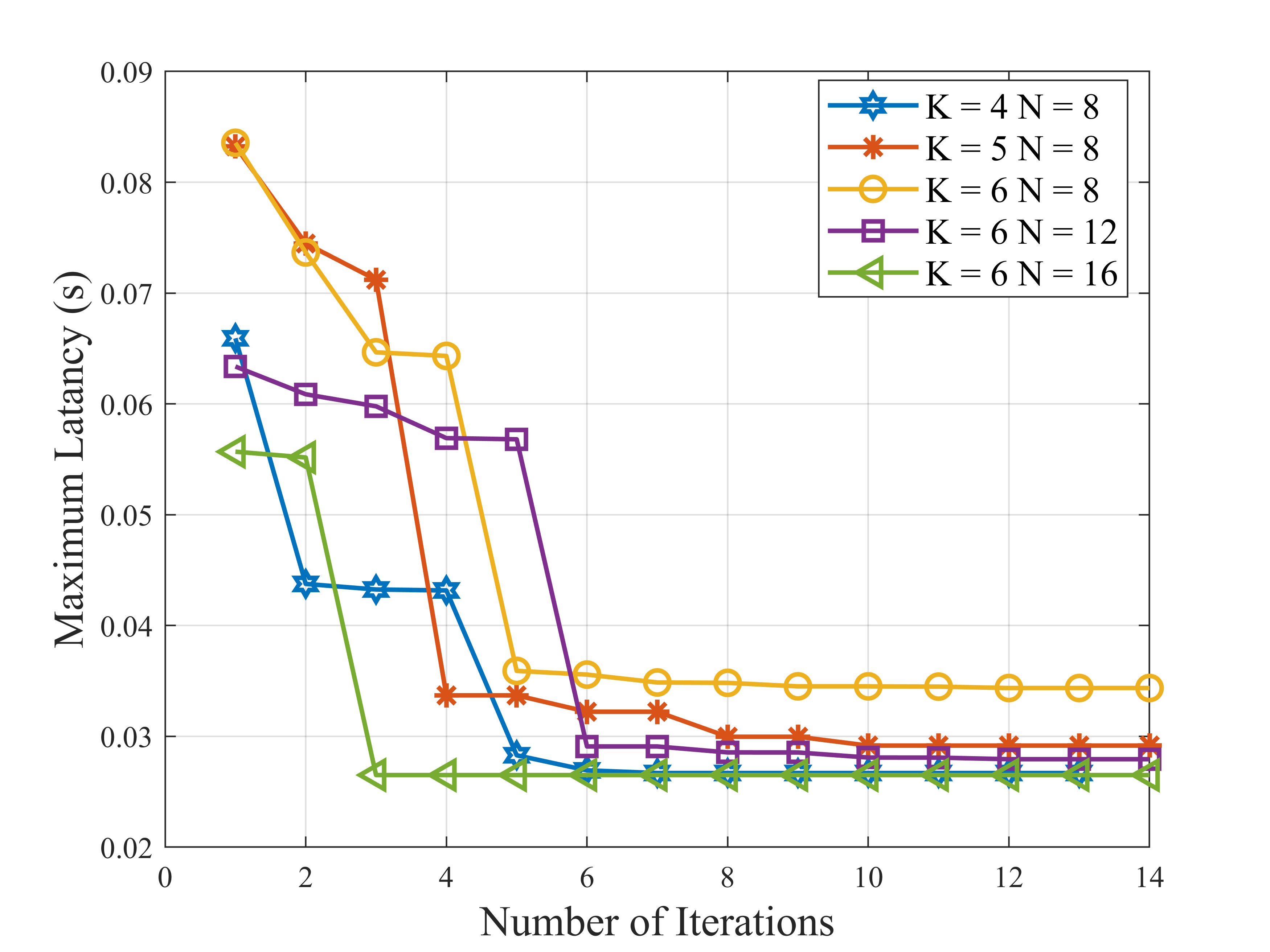
Figure 2: Convergence of our proposed algorithm with $|\mathcal{M}_{k}|=3,\forall k$.

To verify the effectiveness of our proposed algorithm, we depict the maximum latency of each iteration in Fig. 2. The proposed method converges to a local minimum solution rapidly within 10 iterations with various parameter settings. It is worth noting that an increase in the number of APs’ antennas can decrease the maximum latency owing to the enhanced receiving gain. Furthermore, the increasing number of terminals will significantly deteriorate the system performance due to increased interference.

IV-C Effect of Number of Serving APs

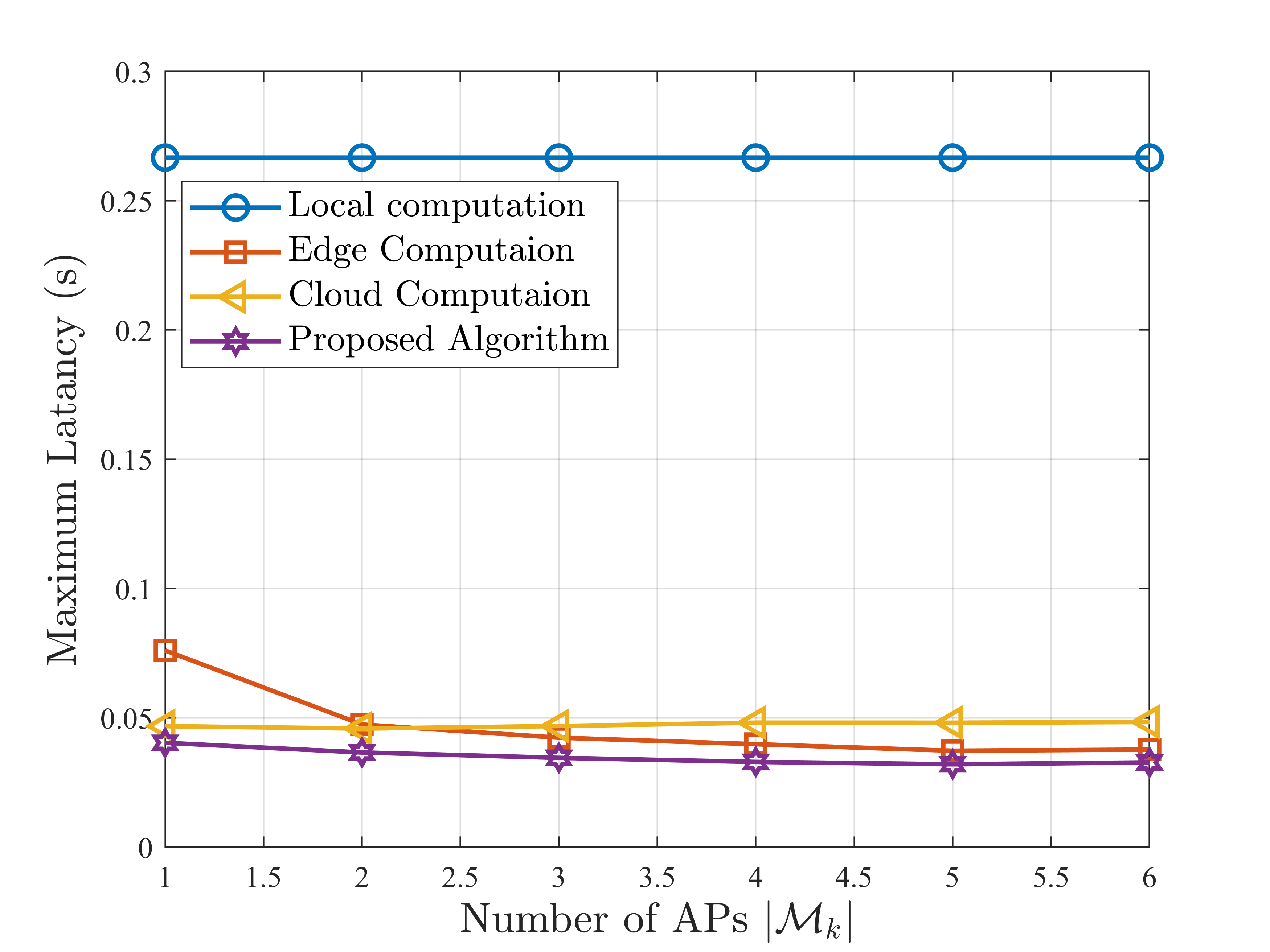
Figure 3: Averaged maximum latency V.S. Cardinality of set $\mathcal{M}_{k}$.

To obtain statistically accurate results, the Monte-Carlo simulation results are obtained by averaging over 100 trials. Fig. 3 depicts the averaged maximum latency with different number of APs that provide service for each terminal. As excepted, our proposed method is superior over all benchmarks. This is because that the proposed method can flexibly schedule the resources of terminals, mobile edge servers, and cloud sever to obtain the cooperative gain, thereby significantly improving the system performance. Furthermore, the computation latency for MEC, CC, and our proposed algorithm decrease with the increasing number of APs that serve the terminals.This is attributed to the implementation of task partitioning, thereby highlighting the superior efficacy of distributed offloading strategies. However, it is worth noting that the computation latency is slightly increased when the number of APs is larger than 5. This is can be explained by the fact that the significant interference would cause performance degradation on communication rate when more APs are involving in offloading resource, which results in longer computation latency. Therefore, it is beneficial to strike a good balance between communication and computation performance.

IV-D Effect of Execution Frequency

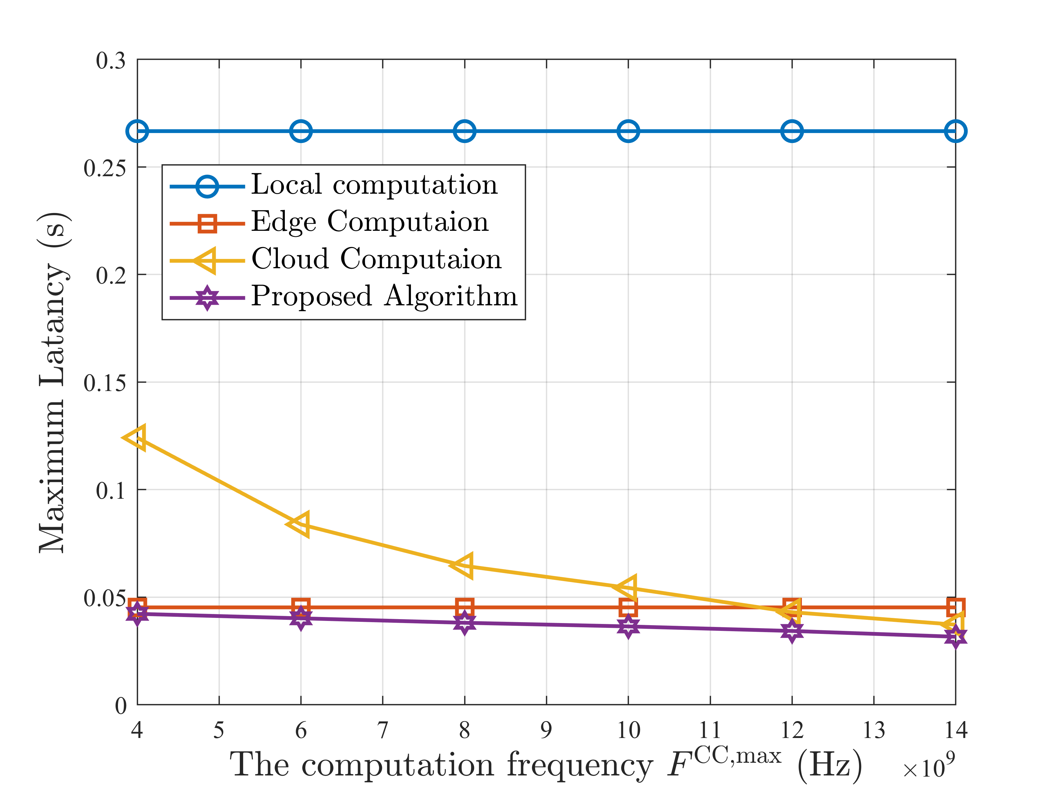
Figure 4: Averaged maximum latency V.S. Execution frequency of cloud server $F^{\text{CC},\max}$ with $|\mathcal{M}_{k}|=3$.

Fig. 4 illustrates the averaged maximum latency under various execution frequency of cloud sever $F^{\text{CC},\max}$. It is observed that the computation latency is decreasing with the increasing execution frequency $F^{\text{CC},\max}$, as more tasks can be offloaded to cloud sever for shorter computation latency. Furthermore, when the frequency $F^{\text{CC},\max}$ is less than 10 GHz, it is more beneficial to execute the tasks via mobile edge severs.

IV-E Effect of Fronthaul Link

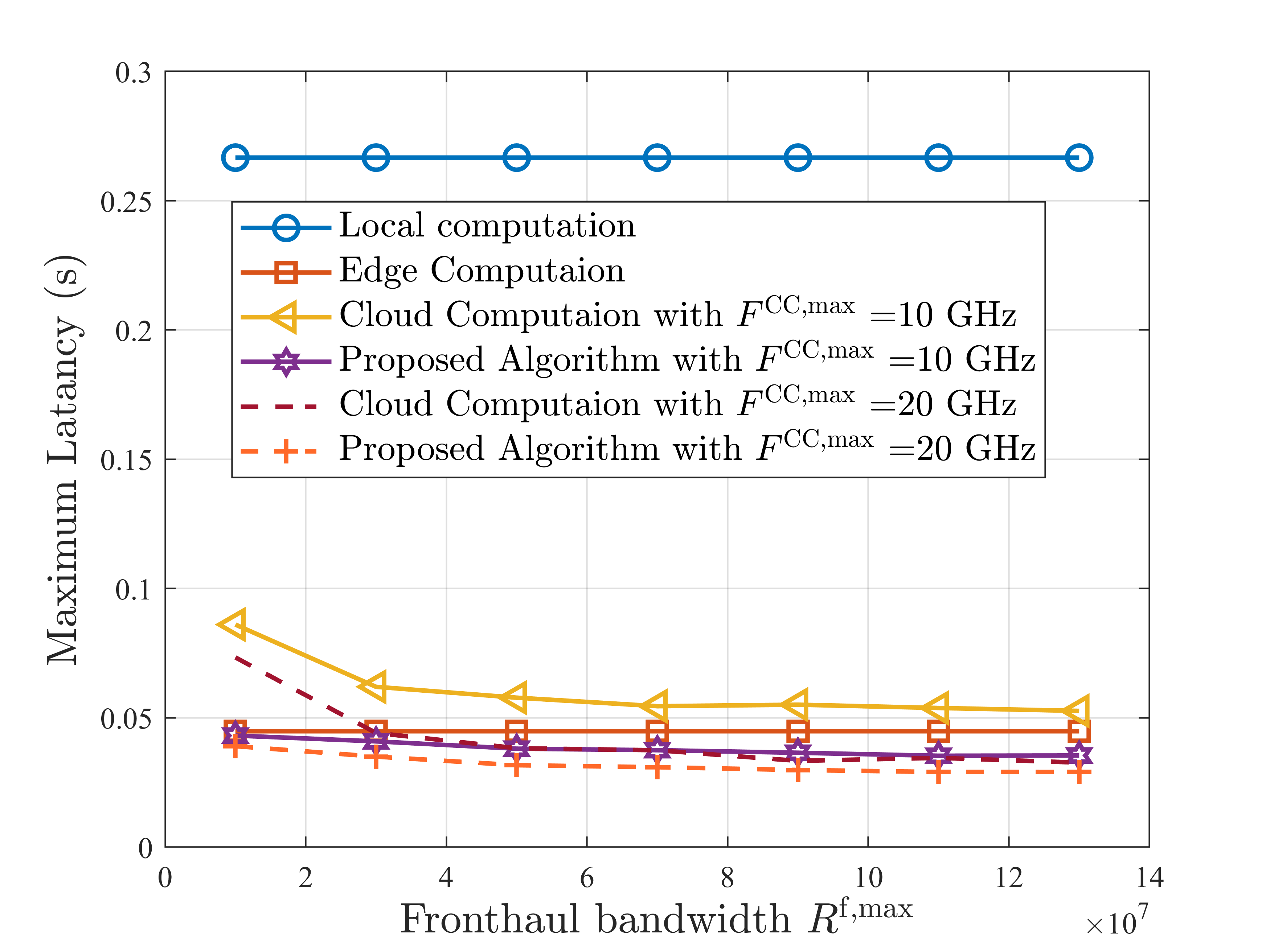
Figure 5: Averaged maximum latency V.S. Fronthaul bandwidth $R^{f,\max}_{m}$ with $|\mathcal{M}_{k}|=3$.

To investigated the impacts of fronthaul bandwidth on the computation latency, Fig. 5 depicts the averaged latency with various fronthaul capacity over 100 trails. As expected, cloud computation latency decreases notably as the available bandwidth between each AP and the CPU increases. This is due to the fact that a large part of this latency comes from transmission delays, particularly when the fronthaul link has limited bandwidth. Furthermore, we observe that more tasks are offloaded to the cloud server once the fronthaul link becomes ideal or effectively unbounded, especially for high execution frequency $F^{\text{CC},\max}$.

IV-F Effect of Sensing Accuracy

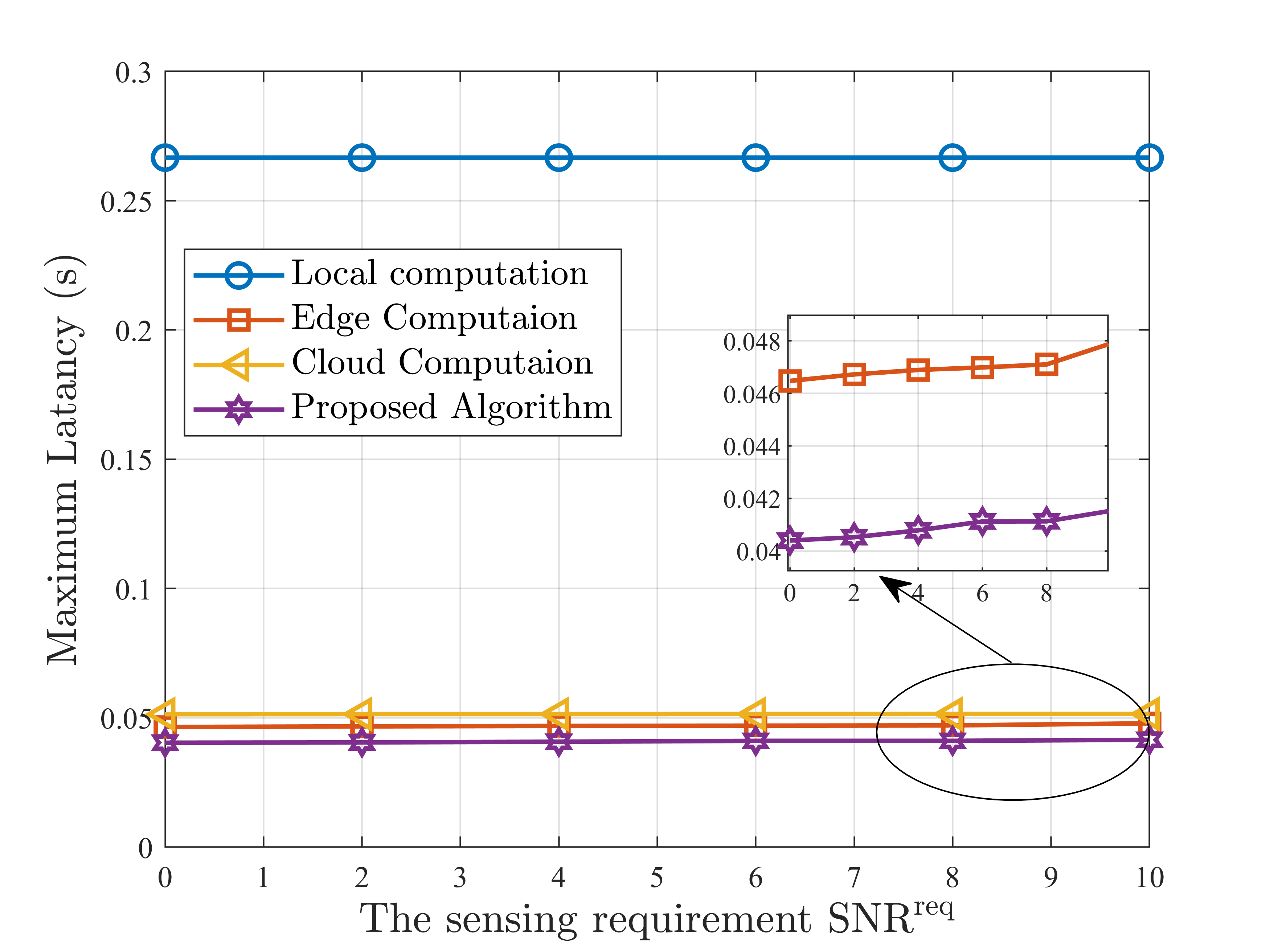
Figure 6: Averaged maximum latency V.S. Sensing requirement $\text{SNR}^{\text{req}}_{k}$ with $|\mathcal{M}_{k}|=3$.

In Fig. 6, we investigate the impacts of sensing requirements on computation latency by averaging over 100 random generation of terminals’ locations. One can observe that the computation latency slight increases with the increasing sensing requirements. This is because that the terminal needs to allocate more power for sensing in order to satisfy the sensing requirements, and thus less power is left for task offloading. This phenomenon also reflects the trade-off between the sensing and communication functionalities in the ISCC system.

IV-G Effect of Number of Antennas

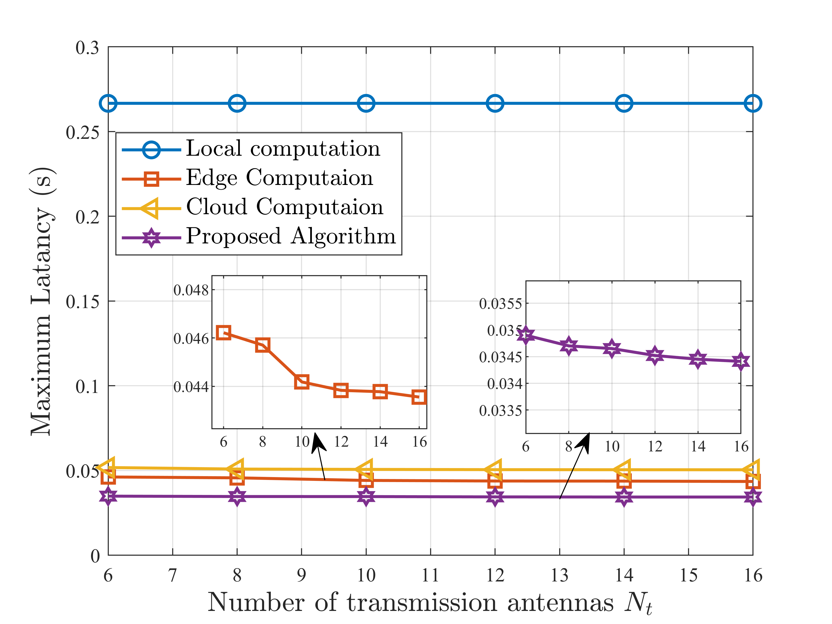
Figure 7: Averaged maximum latency V.S. Number of Antennas $N_{t}$ with $|\mathcal{M}_{k}|=3$.

Fig. 7 depicts the averaged latency with different number of transmission antennas $N_{t}$. As excepted, the latency decreases when the number of antennas increases, owing to the enhanced transmission or receiving gain. Furthermore, we observe that the performance of our proposed method will approach to that with MEC. This is due to the fact that more tasks can be offloaded to mobile edge servers, rather than cloud sever, with the increasing communication rate.

V Conclusion

In this paper, we investigated a cell-free massive MIMO-enabled ICCS system, where the terminals have the option to offload its local task to either mobile edge servers or cloud server. To characterize the benefits of distributed computation, we formulated a mix-integrate programming and non-convex problem to minimize the maximum latency. To tackle this issue, we decomposed it into three sub-problems. By alternatively devising the offloading decision, ISAC beamforming, execution frequency, and fronthaul bandwidth, our proposed algorithm can rapidly converge to a local optimal solution, which has been verified by analysis and numerical results. Furthermore, simulation results demonstrated that the trade-off between communication performance and computation latency, as well as the superiority of our proposed method over other benchmarks, verifying its effectiveness and viability for ICCS applications.

Appendix A Proof of Lemma 1

With the fixed $\mathbf{v}_{k,m}$ and $\mathbf{w}_{k,m}$, the optimal $V_{k,m}$ can be obtained by first-order partial derivative, which is given by

$$\frac{\partial R_{k,m}(V_{k,m})}{\partial V_{k,m}}=(V^{-1}_{k,m})^{T}-\text{MSE}^{T}_{k,m}.$$ (57)

Then, according to the optimal first-order optimality condition, letting $\frac{\partial R_{k,m}(V_{k,m})}{\partial V_{k,m}}$ equal to 0, we obtain the optimal $V_{k,m}=\text{MSE}^{-1}_{k,m}$.

Finally, we complete this proof by substituting the optimal $V^{\text{opt}}_{k,m}$ into (41), and have

$$\begin{split}R_{k,m}&=B\log_{2}(\text{MSE}^{-1}_{k,m})\\ &=B\log_{2}\Big{(}\big{(}1-\mathbf{w}^{H}_{k,m}\mathbf{H}^{H}_{k,m}(\mathbf{N}_{k,m}+\mathbf{H}_{k,m}\mathbf{w}_{k,m}\mathbf{w}^{H}_{k,m}\mathbf{H}_{k,m})^{-1}\mathbf{H}_{k,m}\mathbf{w}_{k,m}\big{)}^{-1}\Big{)}\\ &\overset{a}{=}B\log_{2}(1+\mathbf{w}^{H}_{k,m}\mathbf{H}^{H}_{k,m}(\mathbf{N}_{k,m})^{-1}\mathbf{H}_{k,m}\mathbf{w}_{k,m})\\ &\overset{b}{=}B\log_{2}(\mathbf{I}_{N}+\mathbf{H}_{k,m}\mathbf{w}_{k,m}\mathbf{w}^{H}_{k,m}\mathbf{H}^{H}_{k,m}\mathbf{N}_{k,m}^{-1}),\end{split}$$ (58)

where $a$ is obtained via the Woodbury matrix identity and $b$ relies on the property $\det(\mathbf{I}+\mathbf{AB})=\det(\mathbf{I}+\mathbf{BA})$, respectively.

References

- [1] A. Liu, Z. Huang, M. Li, Y. Wan, W. Li, T. X. Han, C. Liu, R. Du, D. K. P. Tan, J. Lu et al., “A survey on fundamental limits of integrated sensing and communication,” IEEE Commun. Surv. Tutor., vol. 24, no. 2, pp. 994–1034, 2022.
- [2] F. Liu, Y. Cui, C. Masouros, J. Xu, T. X. Han, Y. C. Eldar, and S. Buzzi, “Integrated sensing and communications: Toward dual-functional wireless networks for 6G and beyond,” IEEE J. Sel. Areas commun., vol. 40, no. 6, pp. 1728–1767, 2022.
- [3] J. A. Zhang, M. L. Rahman, K. Wu, X. Huang, Y. J. Guo, S. Chen, and J. Yuan, “Enabling joint communication and radar sensing in mobile networks—a survey,” IEEE Commun. Surv. Tutor., vol. 24, no. 1, pp. 306–345, 2021.
- [4] Y. Fu, C. Li, F. R. Yu, T. H. Luan, and Y. Zhang, “A survey of driving safety with sensing, vehicular communications, and artificial intelligence-based collision avoidance,” Trans. Intell. Transp. Syst., vol. 23, no. 7, pp. 6142–6163, 2021.
- [5] X. Cheng, D. Duan, S. Gao, and L. Yang, “Integrated sensing and communications (ISAC) for vehicular communication networks (VCN),” IEEE Internet Things J., vol. 9, no. 23, pp. 23 441–23 451, 2022.
- [6] F. Khan, M. A. Jan, A. ur Rehman, S. Mastorakis, M. Alazab, and P. Watters, “A secured and intelligent communication scheme for IIoT-enabled pervasive edge computing,” IEEE Trans. Ind. Inform., vol. 17, no. 7, pp. 5128–5137, 2020.
- [7] F. Liu, C. Masouros, A. P. Petropulu, H. Griffiths, and L. Hanzo, “Joint radar and communication design: Applications, state-of-the-art, and the road ahead,” IEEE Trans. Commun., vol. 68, no. 6, pp. 3834–3862, 2020.
- [8] B. Liao, H. Q. Ngo, M. Matthaiou, and P. J. Smith, “Power allocation for massive MIMO-ISAC systems,” IEEE Trans. Wireless Commun., 2024. (Early Access).
- [9] F. Liu, Y.-F. Liu, A. Li, C. Masouros, and Y. C. Eldar, “Cramér-rao bound optimization for joint radar-communication beamforming,” IEEE Trans. Signal Process., vol. 70, pp. 240–253, 2021.
- [10] Y. Xiong, F. Liu, Y. Cui, W. Yuan, T. X. Han, and G. Caire, “On the fundamental tradeoff of integrated sensing and communications under gaussian channels,” IEEE Trans. Inf. Theory., vol. 69, no. 9, pp. 5723–5751, 2023.
- [11] Z. Ren, Y. Peng, X. Song, Y. Fang, L. Qiu, L. Liu, D. W. K. Ng, and J. Xu, “Fundamental CRB-rate tradeoff in multi-antenna ISAC systems with information multicasting and multi-target sensing,” IEEE Trans. Wireless Commun., 2023. (Early Access).
- [12] Z. He, W. Xu, H. Shen, D. W. K. Ng, Y. C. Eldar, and X. You, “Full-duplex communication for isac: Joint beamforming and power optimization,” IEEE J. Sel. Areas Commun., vol. 41, no. 9, pp. 2920–2936, 2023.
- [13] K. Meng, C. Masouros, G. Chen, and F. Liu, “Network-level integrated sensing and communication: Interference management and BS coordination using stochastic geometry,” IEEE Trans. Wireless Commun., 2024.
- [14] N. Babu, C. Masouros, C. B. Papadias, and Y. C. Eldar, “Precoding for multi-cell ISAC: from coordinated beamforming to coordinated multipoint and bi-static sensing,” IEEE Tran. Wireless Commun., 2024.
- [15] W. Mao, Y. Lu, C.-Y. Chi, B. Ai, Z. Zhong, and Z. Ding, “Communication-sensing region for cell-free massive MIMO ISAC systems,” IEEE Trans. Wireless Commun., 2024. (Early Access).
- [16] M. Elfiatoure, M. Mohammadi, H. Q. Ngo, and M. Matthaiou, “Cell-free massive mimo for ISAC: access point operation mode selection and power control,” in Proc. 2023 IEEE Globecom Workshops (GC Wkshps), 2023, pp. 104–109.
- [17] Q. Qi, X. Chen, C. Zhong, and Z. Zhang, “Integrated sensing, computation and communication in B5G cellular internet of things,” IEEE Trans. Wireless Commun., vol. 20, no. 1, pp. 332–344, 2020.
- [18] X. Li, F. Liu, Z. Zhou, G. Zhu, S. Wang, K. Huang, and Y. Gong, “Integrated sensing, communication, and computation over-the-air: MIMO beamforming design,” IEEE Trans. Wireless Commun., vol. 22, no. 8, pp. 5383–5398, 2023.
- [19] C. Ding, J.-B. Wang, H. Zhang, M. Lin, and G. Y. Li, “Joint MIMO precoding and computation resource allocation for dual-function radar and communication systems with mobile edge computing,” IEEE J. Sel. Areas Commun., vol. 40, no. 7, pp. 2085–2102, 2022.
- [20] P. Liu, Z. Fei, X. Wang, J. Huang, J. Hu, and J. A. Zhang, “Joint offloading and beamforming design in integrating sensing, communication, and computing systems: A distributed approach,” IEEE Trans. Commun., 2024. (Early Access).
- [21] Y. Zhao, Q. Wu, W. Chen, Y. Zeng, R. Liu, W. Mei, F. Hou, and S. Ma, “Multi-functional beamforming design for integrated sensing, communication, and computation,” IEEE Trans. Commun., 2024. (Early Access).
- [22] M. Ke, Z. Gao, Y. Wu, X. Gao, and K.-K. Wong, “Massive access in cell-free massive MIMO-based internet of things: Cloud computing and edge computing paradigms,” IEEE J. Sel. Areas Commun., vol. 39, no. 3, pp. 756–772, 2020.
- [23] K. Wang, D. Niyato, W. Chen, and A. Nallanathan, “Task-oriented delay-aware multi-tier computing in cell-free massive MIMO systems,” IEEE J. Sel. Areas Commun., vol. 41, no. 7, pp. 2000–2012, 2023.
- [24] Z. Li, F. Göttsch, S. Li, M. Chen, and G. Caire, “Joint fronthaul load balancing and computation resource allocation in cell-free user-centric massive MIMO networks,” IEEE Trans. Wireless Commun., 2024. (Early Access).
- [25] H. Yu, N. Ye, and A. Wang, “Non-orthogonal wireless backhaul design for cell-free massive MIMO: An integrated computation and communication approach,” IEEE Wireless Commun. Letts., vol. 10, no. 2, pp. 281–285, 2020.
- [26] C. E. Shannon, “A mathematical theory of communication,” Bell Syst. Tech. J., vol. 27, no. 3, pp. 379–423, Jul. 1948.
- [27] X. Liu, T. Huang, N. Shlezinger, Y. Liu, J. Zhou, and Y. C. Eldar, “Joint transmit beamforming for multiuser MIMO communications and MIMO radar,” IEEE Trans. Signal Process., vol. 68, pp. 3929–3944, 2020.
- [28] S. Boyd, “Convex optimization,” Cambridge UP, 2004.
- [29] H. Q. Ngo, A. Ashikhmin, H. Yang, E. G. Larsson, and T. L. Marzetta, “Cell-free massive MIMO versus small cells,” IEEE Trans. Wireless Commun., vol. 16, no. 3, pp. 1834–1850, Mar. 2017.
- [30] Q. Peng, H. Ren, C. Pan, N. Liu, and M. Elkashlan, “Resource allocation for uplink cell-free massive MIMO enabled URLLC in a smart factory,” IEEE Trans. Commun., vol. 71, no. 1, pp. 553–569, Jan. 2022.