General Einstein-Cartan quadratic gravity with derivative couplings

Abstract

Within the framework of Einstein-Cartan gravity we consider an action, containing up to quadratic terms of the Ricci scalar and the Holst invariant, coupled non-minimal to a scalar field, including couplings of its derivatives to curvature. We derive the equivalent metric theory, featuring an extra dynamical pseudoscalar degree of freedom associated with the presence of the Holst term in the action. We study the evolution of the resulting two-field system in a FRW background and show that it evolves rapidly into an effective single-field inflationary model. We find that the model is consistent with the latest observational data for a wide range of its parameters, determining the necessary upper limits on derivative coupling parameters.

1 Introduction

The standard framework of cosmological models is Einstein’s theory of General Relativity (GR) with gravity entering in the action through the Einstein-Hilbert term of scalar curvature. An alternative formulation considers not only the metric but also the connection as an independent variable [1, 2]. This is the metric-affine formulation, which is equivalent to the standard metric formulation as long as we stay with the Einstein-Hilbert action, while the two formulations are not equivalent if we go beyond this action. Nevertheless, there are strong reasons to expect modifications. Gravitating matter fields are sensitive to quantum interactions that will ultimately introduce correction terms in the effective classical theory of gravity. Such terms are non-minimal couplings of matter fields to curvature like $\phi^{2}{\cal{R}}$ [3, 4, 5, 6, 7, 8, 9, 10, 11, 12, 13, 14, 15, 16, 17, 18, 19, 20, 21, 22, 23, 24, 25, 26, 27, 28, 29, 30, 31, 32, 33, 34, 35, 36, 37, 38, 39, 40, 41, 42, 43, 44, 45, 46, 47] or their derivatives like $(\partial_{\mu}\phi)(\partial_{\nu}\phi)\,{\cal{R}}^{\mu\nu}$ [48, 49, 50, 51, 52, 53, 54, 55, 56, 57, 58, 59, 60, 61, 62, 63, 64, 65, 66] or higher powers of the curvature like ${\cal{R}}^{2}$ [67]. Due to these modifications the predictions resulting from the metric-affine framework will be different than those obtained from the standard metric one [68, 69, 70, 71, 72, 73, 74, 75, 76, 77, 78, 79, 80, 81, 82, 83, 84, 85, 86, 87, 88, 89, 90, 91, 92, 93, 94, 95, 96, 97, 98, 99, 100, 101, 102, 103, 104, 105, 106, 107, 108, 109, 110, 111, 112, 113, 114] . Cosmological inflation [115, 116, 117, 118] is presently accepted as the best explanation for the origin of the large scale structure of the Universe, providing the mechanism through which the primordial quantum fluctuations of gravitational and matter fields have been promoted to the cosmological perturbations presently observed [119, 120, 121, 122, 123, 124]. Models of inflation are formulated in terms of a gravitating scalar field, the inflaton, which will in general participate in non-minimal corrections mentions above. The resulting inflationary predictions will be different, depending on whether the standard metric GR or the metric-affine framework are considered.

Ample motivation to consider formulations of gravity beyond the standard metric one is provided by presently existing tensions and questions of cosmology. In the metric-affine gravity the independent connection can be decomposed into the standard Levi-Civita part, arising in the metric case, and a part composed of the torsion and nonmetricity tensors. A special case of the general metric-affine framework is the case of Einstein-Cartan gravity [125, 126], characterized by non-zero torsion and zero nonmetricity. In this framework, apart from the Ricci scalar curvature ${\cal{R}}$, there is also a second linear scalar invariant of the curvature, namely the parity-odd Holst invariant $\tilde{\cal{R}}\sim\tensor{\epsilon}{{}_{\alpha}^{\beta}{}^{\gamma}{}^{\delta}}{\cal{R}}^{\alpha}_{\,\,\beta\gamma\delta}$. It is known that the presence of the Holst invariant signals the presence of a dynamical pseudoscalar degree of freedom in the spectrum [97, 102]. A ghost-free action can be constructed containing at most quadratic terms of these invariants, including non-linear couplings to matter fields. Curvature couplings to derivatives of matter fields can also be written in terms of the Ricci tensor, like $(\partial_{\mu}\phi)(\partial_{\nu}\phi){\cal{R}}^{\mu\nu}$ [127, 128, 113], and are also ghost-free.

In the present article we have considered Einstein-Cartan gravity characterized by non-zero torsion coupled to a scalar field with a quartic self-interaction potential. We employ the most general action quadratic in the curvature, devoid of unphysical degrees of freedom [129, 130, 131, 132, 133, 134], consisting of at most quadratic terms of the Ricci scalar and the Holst invariant as well as non-minimal couplings of the scalar field and its derivatives to both. We transform the theory to the Einstein frame via a disformal transformation and express the resulting metric action in terms of the torsion. Integrating out the torsion the resulting theory describes a pair of scalar fields, namely the original fundamental scalar as well as a pseudoscalar field associated with the Holst invariant. We derive the set of equations of motion and analyze numerically the evolution of the two scalars in a FRW background. We find that the two scalar field system is found to evolves rapidly into an effective single-field system with a non-canonical kinetic term and a potential of the Palatini-$R^{2}$ form that possesses an inflationary plateau at large field values. We analyze the inflationary predictions of the model and in particular the effect of derivative couplings on the resulting values of inflationary observables. In section 2 we give a brief account of the general metric-affine framework of the theory to be considered. In section 3 we introduce the model, writing down the most general action of Einstein-Cartan gravity that includes up to quadratic curvature terms and is devoid of ghosts, coupled to a scalar field $\phi$ non-minimally, including couplings of the kinetic tensor $X_{\mu\nu}=\partial_{\mu}\phi\partial_{\nu}\phi$ to curvature. We procced to transform the theory into the Einstein frame through a disformal transformation. In section 4 we focus on the resulting $\mathcal{O}(X)$ theory, containing no more than quadratic kinetic terms of the scalar $\phi$ as well as the emerging dynamical pseudoscalar that results from the presence of the Holst term. In section 5 we analyze the resulting effective single-field theory. Section 6 is devoted in the study of the inflationary behavior of the model. Finally, in section 7 we briefly summarize our results.

2 Framework

In the framework of Metric-Affine theory of gravity not only the metric $g_{\mu\nu}$ but also the connection $\tensor{\Gamma}{{}_{\mu}^{\rho}{}_{\nu}}$ is an independent variable. The curvature is defined in terms of the connection as

$$\tensor{\mathcal{R}}{{}^{\alpha}_{\beta}{}_{\gamma}{}_{\delta}}=\partial_{\gamma}\tensor{\Gamma}{{}^{\alpha}_{\delta}{}_{\beta}}-\partial_{\delta}\tensor{\Gamma}{{}^{\alpha}_{\gamma}{}_{\beta}}+\tensor{\Gamma}{{}^{\alpha}_{\gamma}{}_{\mu}}\tensor{\Gamma}{{}^{\mu}_{\delta}{}_{\beta}}-\tensor{\Gamma}{{}^{\alpha}_{\delta}{}_{\mu}}\tensor{\Gamma}{{}^{\mu}_{\gamma}{}_{\beta}}\,.$$ (2.1)

The only symmetry of $\tensor{\mathcal{R}}{{}^{\alpha}_{\beta}{}_{\gamma}{}_{\delta}}$ is the antisymmetry under the interchange of the last two indices. There are three distinct two-index contractions given by

$$\tensor{\mathcal{R}}{{}_{\mu}{}_{\nu}}=\tensor{\mathcal{R}}{{}^{\rho}_{\mu}{}_{\rho}{}_{\nu}}\,,\qquad\tensor{\widehat{\mathcal{R}}}{{}^{\mu}_{\nu}}=g^{\alpha\beta}\tensor{\mathcal{R}}{{}^{\mu}_{\alpha}{}_{\beta}{}_{\nu}}\,,\qquad\tensor{\tilde{\mathcal{R}}}{{}_{\mu}{}_{\nu}}=\tensor{\mathcal{R}}{{}^{\alpha}_{\alpha}{}_{\mu}{}_{\nu}}\,,$$ (2.2)

called the Ricci, co-Ricci, and homothetic Ricci tensors. There are two possible curvature scalars derived from the Riemmann tensor, namely the Ricci scalar, determined through an additional contraction of either the Ricci tensor or the co-Ricci tensor,

$$\mathcal{R}=g^{\mu\nu}\tensor{\mathcal{R}}{{}_{\mu}{}_{\nu}}=-\tensor{\widehat{\mathcal{R}}}{{}^{\mu}_{\mu}}\,$$ (2.3)

and the Holst invariant

$$\tilde{\cal{R}}=\tensor{\epsilon}{{}_{\mu}^{\nu}{}^{\rho}{}^{\sigma}}\tensor{\mathcal{R}}{{}^{\mu}_{\nu}{}_{\rho}{}_{\sigma}}=g_{\mu\alpha}\epsilon^{\alpha\nu\rho\sigma}\tensor{\mathcal{R}}{{}^{\mu}_{\nu}{}_{\rho}{}_{\sigma}}=\frac{1}{\sqrt{-g}}g_{\alpha\mu}\varepsilon^{\alpha\nu\rho\sigma}\tensor{\mathcal{R}}{{}^{\mu}_{\nu}{}_{\rho}{}_{\sigma}}.$$ (2.4)

The torsion tensor $\tensor{T}{{}^{\rho}_{\mu}{}_{\nu}}$ is defined as

$$\tensor{T}{{}^{\rho}_{\mu}{}_{\nu}}\,=\,\tensor{\Gamma}{{}^{\rho}_{\mu}{}_{\nu}}\,-\tensor{\Gamma}{{}^{\rho}_{\nu}{}_{\mu}}\,.$$ (2.5)

The torsion vanishes in the metric case, where the connection is fixed by the Levi-Civita relation to be symmetric in its lower indices. In addition to the non-zero torsion the metric-affine framework is also characterized in general by the non-metricity tensor, defined as

$$Q_{\rho\mu\nu}\,=\,\nabla_{\rho}g_{\mu\nu}\,=\,\partial_{\rho}g_{\mu\nu}-\tensor{\Gamma}{{}^{\sigma}_{\rho}{}_{\mu}}g_{\sigma\nu}-\tensor{\Gamma}{{}^{\sigma}_{\rho}{}_{\nu}}g_{\sigma\mu}\,.$$ (2.6)

While the curvature measures the change of a vector under rotation after parallel transport in a closed loop, the torsion measures the non-closure of parallelograms formed from parallel -transported vectors. Finally, the non-metricity measures the change of the length of parallel-transported vectors. From the torsion tensor we may define a torsion vector $T_{\mu}$ and an torsion axial vector $\hat{T}_{\mu}$ [2, 135, 136, 41] as

$$T_{\mu}\,\equiv\,\tensor{T}{{}^{\nu}_{\mu}{}_{\nu}},\,\,\,\,\,\,\,\hat{T}_{\mu}=\tensor{\epsilon}{{}_{\mu}^{\nu}{}^{\rho}{}^{\sigma}}T_{\nu\rho\sigma}\,.$$ (2.7)

In terms of them we can write the torsion as

$$T_{\alpha\beta\gamma}=t_{\alpha\beta\gamma}-\frac{1}{3}\Big{(}g_{\alpha\beta}T_{\gamma}-g_{\alpha\gamma}T_{\beta}\Big{)}+\frac{1}{6}\epsilon_{\alpha\beta\gamma\nu}\hat{T}^{\nu}\,,$$ (2.8)

where $t_{\alpha\beta\gamma}$ is a purely tensorial part satisfying

$$g^{\mu\nu}t_{\mu\rho\nu}=\epsilon^{\rho\sigma\mu\nu}t_{\sigma\mu\nu}=0\,.$$ (2.9)

Similarly, we may define the non-metricity vectors $Q_{\mu}$ and $\hat{Q}_{\mu}$ as

$$Q_{\mu}\,\equiv\,\tensor{Q}{{}_{\mu}^{\nu}{}_{\nu}}\,\,,\,\,\,\,\,\,\,\hat{Q}_{\mu}\,\equiv\,\tensor{Q}{{}^{\nu}_{\nu}{}_{\mu}}\,.$$ (2.10)

The non-metricity tensor can be written in terms of them as

$$Q_{\alpha\beta\gamma}=q_{\alpha\beta\gamma}+\frac{1}{18}\Big{[}g_{\beta\gamma}(5Q_{\alpha}-2\hat{Q}_{\alpha})+4g_{\alpha\beta}\hat{Q}_{\gamma}+4g_{\alpha\gamma}\hat{Q}_{\beta}-g_{\alpha\beta}Q_{\gamma}-g_{\alpha\gamma}Q_{\beta}\Big{]}\,,$$ (2.11)

where $q_{\alpha\beta\gamma}$ is a purely tensorial part satisfying

$$g^{\alpha\beta}q_{\gamma\alpha\beta}=g^{\alpha\beta}q_{\alpha\gamma\beta}=0\,\,.$$ (2.12)

The connection $\Gamma^{\alpha}_{\,\beta\gamma}$ can be decomposed in terms of these vectors as

$$\begin{split}\tensor{\Gamma}{{}^{\alpha}_{\beta}{}_{\gamma}}&=\tensor{\Gamma}{{}^{\alpha}_{\beta}{}_{\gamma}}(g)\,+\,\frac{1}{2}\Bigg{(}-\tensor{\delta}{{}^{\alpha}_{\beta}}\Big{(}\frac{1}{18}\Big{(}5Q_{\gamma}-2\hat{Q}_{\gamma}\Big{)}+\frac{2}{3}T_{\gamma}\Big{)}+g_{\beta\gamma}\Big{(}\frac{1}{18}\Big{(}7Q^{\alpha}-10\hat{Q}^{\alpha}\Big{)}+\frac{2}{3}T^{\alpha}\Big{)}\\ &-\tensor{\delta}{{}^{\alpha}_{\gamma}}\frac{1}{18}\left(5Q_{\beta}-2\hat{Q}_{\beta}\right)+\frac{1}{6}\tensor{\epsilon}{{}^{\alpha}_{\beta}{}_{\gamma}{}_{\delta}}\hat{T}^{\delta}+\tau_{\beta\,\,\,\,\gamma}^{\,\,\,\alpha}\Bigg{)}\end{split}$$ (2.13)

where $\tensor{\Gamma}{{}^{\alpha}_{\beta}{}_{\gamma}}(g)$ is the Levi-Civita connection and

$$\tau_{\beta\alpha\gamma}=q_{\alpha\beta\gamma}-q_{\gamma\alpha\beta}-q_{\beta\alpha\gamma}+t_{\alpha\beta\gamma}+t_{\gamma\alpha\beta}+t_{\beta\alpha\gamma}$$ (2.14)

is the overall purely tensorial part. Substituting the above expression of the connection into the Riemann tensor we obtain an expression of it in terms of the metric Riemann tensor $\tensor{R}{{}^{\alpha}_{\beta}{}_{\gamma}{}_{\delta}}(g)$ and $T,\,\hat{T},\,Q,\,\hat{Q},\,\tau$’s.

In the case of the Einstein-Cartan theory of gravity, characterized only by non-zero torsion, $Q,\,q$ are set to zero. We also set the tensorial part $t_{\alpha\beta\gamma}$ to zero, avoiding the occurence of unphysical degrees of freedom associated with it [133, 137]. In this case the Riemann tensor is

$$\begin{split}\tensor{\mathcal{R}}{{}^{\alpha}_{\beta}{}_{\gamma}{}_{\delta}}&=\tensor{R}{{}^{\alpha}_{\beta}{}_{\gamma}{}_{\delta}}(g)-\frac{1}{3}\tensor{\delta}{{}^{\alpha}_{\delta}}\nabla_{\gamma}T_{\beta}+\frac{1}{3}g_{\beta\delta}\nabla_{\gamma}T^{\alpha}-\frac{1}{12}\tensor{\epsilon}{{}_{\delta}^{\alpha}{}_{\beta}{}_{\nu}}\nabla_{\gamma}\hat{T}^{\nu}+\frac{1}{3}\tensor{\delta}{{}^{\alpha}_{\gamma}}\nabla_{\delta}T_{\beta}-\frac{1}{3}g_{\beta\gamma}\nabla_{\delta}T^{\alpha}\\ &+\frac{1}{12}\tensor{\epsilon}{{}_{\gamma}^{\alpha}{}_{\beta}{}_{\nu}}\nabla_{\delta}\hat{T}^{\nu}+\frac{1}{9}\tensor{\delta}{{}^{\alpha}_{\gamma}}T_{\beta}T_{\delta}-\frac{1}{9}g_{\beta\delta}\tensor{\delta}{{}^{\alpha}_{\gamma}}T^{2}+\frac{1}{36}\tensor{\epsilon}{{}_{\delta}^{\mu}{}_{\beta}{}_{\lambda}}\tensor{\delta}{{}^{\alpha}_{\gamma}}T_{\mu}\hat{T}^{\lambda}-\frac{1}{9}g_{\gamma\delta}T^{\alpha}T_{\beta}\\ &+\frac{1}{9}g_{\beta\delta}T^{\alpha}T_{\gamma}-\frac{1}{36}\tensor{\epsilon}{{}_{\delta}{}_{\gamma}{}_{\beta}{}_{\lambda}}T^{\alpha}\hat{T}^{\lambda}+\frac{1}{36}\tensor{\epsilon}{{}_{\gamma}^{\alpha}{}_{\delta}{}_{\nu}}T_{\beta}\hat{T}^{\nu}-\frac{1}{36}\tensor{\epsilon}{{}_{\gamma}^{\alpha}{}_{\mu}{}_{\nu}}g_{\beta\delta}T^{\mu}\hat{T}^{\nu}-\frac{1}{9}\tensor{\delta}{{}^{\alpha}_{\delta}}T_{\beta}T_{\gamma}\\ &+\frac{1}{9}g_{\beta\gamma}\tensor{\delta}{{}^{\alpha}_{\delta}}T^{2}-\frac{1}{36}\tensor{\epsilon}{{}_{\gamma}^{\mu}{}_{\beta}{}_{\lambda}}\tensor{\delta}{{}^{\alpha}_{\delta}}T_{\mu}\hat{T}^{\lambda}+\frac{1}{9}g_{\gamma\delta}T^{\alpha}T_{\beta}-\frac{1}{9}g_{\beta\gamma}T^{\alpha}T_{\delta}+\frac{1}{36}\tensor{\epsilon}{{}_{\gamma}{}_{\delta}{}_{\beta}{}_{\lambda}}T^{\alpha}\hat{T}^{\lambda}\\ &-\frac{1}{36}\tensor{\epsilon}{{}_{\delta}^{\alpha}{}_{\gamma}{}_{\nu}}T_{\beta}\hat{T}^{\nu}+\frac{1}{36}\tensor{\epsilon}{{}_{\delta}^{\alpha}{}_{\mu}{}_{\nu}}g_{\beta\gamma}T^{\mu}\hat{T}^{\nu}-\frac{1}{144}\tensor{\epsilon}{{}_{\delta}^{\alpha}{}_{\mu}{}_{\nu}}\tensor{\epsilon}{{}_{\gamma}^{\mu}{}_{\beta}{}_{\lambda}}\hat{T}^{\nu}\hat{T}^{\lambda}+\frac{1}{144}\tensor{\epsilon}{{}_{\gamma}^{\alpha}{}_{\mu}{}_{\nu}}\tensor{\epsilon}{{}_{\delta}^{\mu}{}_{\beta}{}_{\lambda}}\hat{T}^{\nu}\hat{T}^{\lambda}\end{split}{}$$ (2.15)

3 Einstein-Cartan quadratic gravity with derivative couplings

As we discussed in the introduction the quantum interactions of gravitating matter fields are bound to generate corrections to the Hilbert-Einstein gravitational action. These modifications can be non-minimal couplings of matter fields and their derivatives to curvature, like $f(\phi){\cal{R}}$, $g(\phi)\tilde{\cal{R}}$, $(\partial^{\mu}\phi)(\partial^{\nu}\phi){\cal{R}}_{\mu\nu}$, or higher powers of the curvature, like ${\cal{R}}^{2}$, $\tilde{\cal{R}}^{2}$. We proceed to write down an effective theory of gravity coupled to a scalar field that is at most quadratic in powers of the curvature and ghost free. Therefore, we consider the action (in reduced Planck mass units)

$$\begin{split}{\cal{S}}\,=\,\int\,{\rm d}^{4}x\,\sqrt{-g}\,\Bigg{\{}\,&\frac{1}{2}f(\phi){\cal{R}}\,+\,\frac{1}{2}g(\phi)\tilde{\cal{R}}\,+\,\frac{1}{2}\alpha_{1}X{\cal{R}}\,-\frac{1}{2}K(\phi)X-V(\phi).\\ &+\alpha_{2}{\cal{R}}^{\mu\nu}X_{\mu\nu}\,+\,\alpha_{3}\hat{R}^{\mu\nu}X_{\mu\nu}\,\,+\,\frac{\beta}{4}{\cal{R}}^{2}\,+\,\frac{\delta}{4}\tilde{\cal{R}}^{2}\Bigg{\}}\end{split}{}$$ (3.1)

where $X_{\mu\nu}=(\partial_{\mu}\phi)(\partial_{\nu}\phi)$ and $X=(\partial\phi)^{2}$. An extra term $\alpha_{4}\,X\tilde{\cal{R}}$ is also possible under our assumptions but we ignore it, since it corresponds to a hard breaking of parity. The action (3.1) can be rewritten in terms of two auxiliary fields $\chi$ and $\zeta$ as

$$\begin{split}{\cal{S}}\,=\,\int\,{\rm d}^{4}x\,\sqrt{-g}\,\Bigg{\{}\,&\frac{1}{2}\left({\cal{F}}(\phi,\,\chi)+\alpha_{1}X\right){\cal{R}}\,+\,\frac{1}{2}{\cal{G}}(\phi,\,\zeta)\tilde{\cal{R}}\\ &-\frac{1}{2}K(\phi)X\,-U(\phi,\,\chi,\,\zeta)\,+\,\alpha_{2}{\cal{R}}^{\mu\nu}X_{\mu\nu}\,+\,\alpha_{3}\overline{\mathcal{R}}^{\mu\nu}X_{\mu\nu}\,\Bigg{\}}\end{split}{}$$ (3.2)

where

$$\begin{split}{\cal{F}}(\phi,\chi)=f(\phi)+\beta\chi\,,\,\,\,\,\,\,\,\,{\cal{G}}(\phi,\,\zeta)\,=\,g(\phi)+\delta\zeta\\ \,\\ U(\phi,\,\chi,\,\zeta)\,=\,V(\phi)+\frac{\beta}{4}\chi^{2}\,+\,\frac{\delta}{4}\zeta^{2}\end{split}$$ (3.3)

We have replaced the coupling to the co-Ricci tensor in (3.1) with a coupling to the so-called average Ricci tensor $\overline{R}_{\mu\nu}=\left(R_{\mu\nu}+\hat{R}_{\mu\nu}\right)/2$, which vanishes if the theory is metric compatible. Therefore, focusing on the Einstein-Cartan framework of gravity, we may eliminate the coupling $\alpha_{3}$ in (3.2).

In order to transform the action to the Einstein frame we need to employ a disformal transformation [128] $g_{\mu\nu}\rightarrow\,\tilde{g}_{\mu\nu}$, defined by

$$g_{\mu\nu}=\gamma_{1}(\phi,\,\tilde{X})\tilde{g}_{\mu\nu}+\gamma_{2}(\phi,\tilde{X})X_{\mu\nu},\,\,\,\,\,\,\,\,\,\,\,\tilde{g}_{\mu\nu}=\tilde{\gamma}_{1}(\phi,X)g_{\mu\nu}+\tilde{\gamma}_{2}(\phi,X)X_{\mu\nu}\,,$$ (3.4)

parametrized by the functions $\gamma_{1}$ and $\gamma_{2}$. Note that $\tilde{\gamma}_{1}=\gamma_{1}^{-1},\,\tilde{\gamma}_{2}=-\gamma_{2}/\gamma_{1}$ and $X=\tilde{X}\left(\gamma_{1}(\phi,\tilde{X})+\gamma_{2}(\phi,\tilde{X})\tilde{X}\right)^{-1}$ and $\tilde{X}=X\left(\tilde{\gamma}_{1}(\phi,X)+\tilde{\gamma}_{2}(\phi,X)X\right)^{-1}$.

Applying the disformal transformation on the action (3.2) we obtain

$$\begin{split}{\cal{S}}=\int\,{\rm d}^{4}x\,\sqrt{-g}\Bigg{\{}\,&\frac{1}{2}F_{1}{\cal{R}}+F_{2}\overline{\cal{R}}^{\mu\nu}X_{\mu\nu}+F_{3}{\cal{R}}^{\mu\nu}X_{\mu\nu}\\ &+F_{4}\tilde{\cal{R}}+F_{5}X_{\alpha\mu}\epsilon^{\mu\beta\gamma\delta}{\cal{R}}^{\alpha}_{\,\,\beta\gamma\delta}-F_{6}X-F_{7}U\Bigg{\}}\end{split}$$ (3.5)

For simplicity of notation we have omitted the tildes. The coefficient functions are ($\gamma\equiv\frac{\gamma_{2}}{\gamma_{1}}$)

$$\begin{split}&F_{1}(\phi,X,\chi)=(1+\gamma X)^{1/2}\Big{(}\gamma_{1}\mathcal{F}(\phi,X)+\frac{\alpha_{1}X}{1+\gamma X}\Big{)}\\ &F_{2}(\phi,X)=\alpha_{3}(1+\gamma X)^{-1/2}\\ &F_{3}(\phi,X,\chi)=\frac{1}{2}(1+\gamma X)^{-1/2}\Big{(}-\gamma_{2}\mathcal{F}(\phi,X)+\frac{\alpha_{2}-\alpha_{3}-(\alpha_{1}+\alpha_{3})\gamma X}{1+\gamma X}\Big{)}\\ &F_{4}(\phi,\zeta,X)=\frac{1}{2}\gamma_{1}\mathcal{G}(\phi,\zeta)=\frac{F_{5}(\phi,\zeta)}{\gamma}\\ &F_{6}(\phi,X)=\frac{1}{2}\gamma_{1}(1+\gamma X)^{-1/2}K(\phi)\\ &F_{7}(\phi,X,\chi)=\gamma_{1}^{2}(1+\gamma X)^{1/2}\end{split}$$ (3.6)

From now on we shall focus on the case of Einstein-Cartan gravity. This corresponds to setting $\alpha_{3}$ to zero. The Einstein frame is defined by the two conditions

$$\begin{split}&F_{1}(\phi,X,\chi)=(1+\gamma X)^{1/2}\Big{(}\gamma_{1}\mathcal{F}(\phi,X)+\frac{\alpha_{1}X}{1+\gamma X}\Big{)}\,=\,1\\ &F_{3}(\phi,X,\chi)=\frac{1}{2}(1+\gamma X)^{-1/2}\Big{(}-\gamma_{2}\mathcal{F}(\phi,X)+\frac{\alpha_{2}-\alpha_{3}-(\alpha_{1}+\alpha_{3})\gamma X}{1+\gamma X}\Big{)}\,=\,0\end{split}{}$$ (3.7)

The conditions (3.7) determine the parametric functions of the disformal transformation. Assuming that the kinetic function is not too large, we may obtain to $O(X)$

$$\gamma\simeq\alpha_{2}-\frac{\alpha_{2}^{2}}{2}X\,,\quad\gamma_{1}\simeq\frac{1}{\mathcal{F}(\phi,\chi)}\left(1-(\alpha_{1}+\alpha_{2}/2)X\right)\,,$$ (3.8)

The resulting Einstein frame action now is

$${\cal{S}}=\int\,{\rm d}^{4}x\,\sqrt{-g}\Bigg{\{}\,\frac{1}{2}{\cal{R}}+F_{4}\tilde{\cal{R}}+F_{5}X_{\alpha\mu}\epsilon^{\mu\beta\gamma\delta}{\cal{R}}^{\alpha}_{\,\,\beta\gamma\delta}-F_{6}X-F_{7}U\Bigg{\}}{}$$ (3.9)

Next, we can substitute in (3.9) the expression of the curvature in terms of the torsion (2.15) as well as the curvature scalars

$$\begin{split}&{\cal{R}}=R(g)+2\nabla_{\mu}T^{\mu}-\frac{2}{3}T_{\mu}T^{\mu}+\frac{1}{24}\hat{T}_{\mu}\hat{T}^{\mu}\\ &\tilde{\cal{R}}=\frac{2}{3}T_{\mu}\hat{T}^{\mu}-\nabla_{\mu}\hat{T}^{\mu}\end{split}$$ (3.10)

where $R[g]$ is the standard metric Ricci scalar in terms of the Levi-Civita connection. We obtain the Einstein frame action in a standard metric form as

$$\begin{split}\mathcal{S}&=\int{\rm d}^{4}x\sqrt{-g}\Bigg{\{}\frac{1}{2}R-\frac{1}{3}T^{2}+\frac{1}{48}\hat{T}^{2}+\frac{2}{3}F_{4}T\cdot\hat{T}+(\nabla F_{4})\cdot\hat{T}+\frac{1}{3}\nabla_{\mu}(F_{5}X)\hat{T}^{\mu}\\ &-\frac{1}{3}\nabla_{\mu}(\tensor{X}{{}^{\mu}_{\nu}}F_{5})\hat{T}^{\nu}+\frac{2}{9}F_{5}X_{\mu\nu}T^{\mu}\hat{T}^{\nu}+\frac{1}{9}F_{5}XT\cdot\hat{T}-\frac{1}{2}\gamma_{1}(1+\gamma X)^{-1/2}K(\phi)X\\ &-\gamma_{1}^{2}(1+\gamma X)^{1/2}U(\phi,\chi,\zeta)\Bigg{\}}\end{split}{}$$ (3.11)

Varying with respect to the torsion vectors we obtain the algebraic system of equations

$$\begin{split}&T_{\mu}=\Big{(}F_{4}+\frac{1}{6}F_{5}X\Big{)}\hat{T}_{\mu}+\frac{1}{3}F_{5}X_{\mu\nu}\hat{T}^{\nu}\\ \\ &\frac{1}{16}\hat{T}_{\mu}+\Big{(}F_{4}+\frac{1}{6}F_{5}X\Big{)}T_{\mu}+\frac{1}{3}F_{5}X_{\mu\nu}T^{\nu}=E_{\mu}\end{split}$$ (3.12)

where $E_{\mu}$ is

$$E=-\frac{3}{2}\nabla(F_{4}-\frac{X}{3}F_{5})-\frac{1}{2}\nabla\cdot(F_{5}X)\,.{}$$ (3.13)

The corresponding solutions for $T_{\mu},\,\hat{T}_{\mu}$ are given in the Appendix. Substituting back into the action (3.11), which is given in (A.3) of the Appendix.

The starting action contained three scalar field variables, namrely $\phi,\,\chi,\,\zeta$. In the final action (A.3) the appearing scalar variables are $\phi,\,\chi,\,\zeta,\,F_{4},\,F_{5}$. Only three of them are independent due to the relations

$$F_{4}=\frac{1}{2}\left(g(\phi)+\delta\zeta\right)\gamma_{1},\,\,F_{5}=\frac{1}{2}\left(g(\phi)+\delta\zeta\right)\gamma_{2}=F_{4}\frac{\gamma_{2}}{\gamma_{1}}\,.$$ (3.14)

$\zeta$ can be replaced by $F_{4}$ and $\phi$ through the relation

$$\zeta\,=\,\delta^{-1}\left(-g(\phi)+\frac{2}{\gamma_{1}}F_{4}\right)\,.$$ (3.15)

Out of the three independent scalars only $F_{4}$ and $\phi$ possess kinetic terms, while $\chi$ is an auxiliary field that can be replaced by substituting into the action its algebraic equation of motion. Note that the dynamical scalar $F_{4}$, which from now on we shall denote with the symbol $\sigma$, was not a part of the starting matter action, which contained only $\phi$, but is of gravitational origin, arising from the presence of the Holst quadratic term in the action.

4 The ${\cal{O}}(X)$ theory

In order to simplify notation we shall denote $F_{4}=\sigma$ (then, $F_{5}=\gamma\sigma$). The action, shown in (A.7) of the Appendix consists of a purely kinetic piece, depending only on $\sigma$ and $\phi$, namely

$$\begin{split}{\cal{S}}_{I}&=\int\,{\rm d}^{4}x\,\sqrt{-g}\Bigg{\{}\frac{-12+64(\alpha_{2}X-3)\sigma^{2}}{(1+16\sigma^{2})^{2}}(\nabla_{\mu}\sigma)^{2}-\frac{384\sigma^{2}}{(1+16\sigma^{2})^{2}}X^{\mu\nu}\nabla_{\mu}\sigma\nabla_{\nu}\sigma\\ \\ &+\frac{\left(-8+\sigma+32\sigma^{2}(-20+\sigma+8\sigma^{2}\right)\alpha_{2}}{(1+16\sigma^{2})^{2}}\Big{(}\nabla_{\mu}\sigma\nabla^{\mu}(\sigma X)-\nabla_{\mu}(X^{\mu\nu}\sigma)\nabla_{\nu}\sigma\Big{)}\,\,+\,O(X^{2})\,\Bigg{\}}\end{split}$$ (4.1)

and of a part consisting of all three scalars, namely

$${\cal{S}}_{II}=\int\,{\rm d}^{4}x\,\sqrt{-g}\Bigg{\{}-\frac{1}{2}\gamma_{1}(1+\gamma X)^{-1/2}K(\phi)X-\gamma_{1}^{2}(1+\gamma X)^{1/2}U\Bigg{\}}$$ (4.2)

or

$$\begin{split}\mathcal{S}_{II}=\int\,{\rm d}^{4}x\,\sqrt{-g}\Bigg{\{}&-\frac{1}{2}\frac{\left(1-(\alpha_{1}+\alpha_{2}/2)X\right)}{\left(f(\phi)+\beta\chi\right)}(1+\alpha_{2}X)^{-1/2}K(\phi)X\\ &-\frac{\left(1-(\alpha_{1}+\alpha_{2}/2)X\right)^{2}}{\left(f(\phi)+\beta\chi\right)^{2}}(1+\alpha_{2}X)^{1/2}U(\phi,\,\sigma,\,\chi)\Bigg{\}}\end{split}$$ (4.3)

where

$$U(\phi,\sigma,\,\chi)=V(\phi)+\frac{\beta}{4}\chi^{2}+\frac{1}{4\delta}\left(\frac{2\sigma\left(f(\phi)+\beta\chi\right)}{\left(1-(\alpha_{1}+\alpha_{2}/2)X\right)}-g(\phi)\right)^{2}$$ (4.4)

At this point we can consider the equation of motion for the auxiliary field $\frac{\delta{\cal{S}}}{\delta\chi}=0$ having in mind that we seek for an $\mathcal{O}(X)$ solution. We obtain

$$\begin{split}&0=-\frac{\beta}{2}f(\phi)\chi-\frac{\beta}{\delta}\sigma g(\phi)(f(\phi)+\beta\chi)+2\beta V+\frac{\beta}{2\delta}g^{2}(\phi)\\ &+X\Bigg{\{}\frac{\beta}{2}K(\phi)(f(\phi)+\beta\chi)-\frac{\beta\hat{\alpha}^{\prime}}{\delta}\sigma g(\phi)(f(\phi)+\beta\chi)+\frac{\hat{\alpha}\beta}{2}\chi f(\phi)\\ &+\frac{\hat{\alpha}\beta}{\delta}\sigma(f(\phi)+\beta\chi)g(\phi)-2\beta\hat{\alpha}V(\phi)-\frac{\hat{\alpha}\beta}{2\delta}g^{2}(\phi)\Bigg{\}}\end{split}{}$$ (4.5)

The zeroth-order solution is

$$\chi_{0}=\frac{4V(\phi)-\frac{2\sigma}{\delta}f(\phi)g(\phi)+\frac{g^{2}(\phi)}{\delta}}{f(\phi)+\frac{2\beta\sigma}{\delta}g)(\phi)}{}$$ (4.6)

Next, we insert in (4.5) a perturbative Ansatz $\chi\,=\,\chi_{0}\,+\,X\,\chi_{1}$ and obtain the correction ($\hat{\alpha}^{\prime}=\alpha_{1}+\alpha_{2}/2$)

$$\chi_{1}\,=\,\frac{\left(f^{2}(\phi)+4\beta V+\frac{\beta}{\delta}g^{2}(\phi)\right)\left(K(\phi)-2\hat{\alpha}^{\prime}\frac{\beta}{\delta}\sigma g(\phi)\right)}{\left(f(\phi)+2\frac{\beta}{\delta}\sigma g(\phi)\right)^{2}}\,{}\,.$$ (4.7)

Substituting the solution for $\chi$ to the $\mathcal{S}_{II}$, given in (A.6), and combining the result with the kinetic action ${\cal{S}}_{I}$, we arrive at the complete $\mathcal{O}(X)$ action

$$\begin{split}\mathcal{S}=\int{\rm d}^{4}x\sqrt{-g}\Bigg{\{}&\frac{1}{2}R-\frac{1}{2}\mathcal{K}_{1}(\phi,\sigma)X-\frac{1}{2}\mathcal{K}_{2}(\sigma,X)(\nabla_{\mu}\sigma)^{2}-\mathcal{K}_{3}(\sigma)X^{\mu\nu}\nabla_{\mu}\sigma\nabla_{\nu}\sigma+\mathcal{K}_{4}(\sigma)\nabla_{\mu}\sigma\nabla^{\mu}(\sigma X)\\ &-\mathcal{K}_{5}(\sigma)\nabla_{\mu}(\sigma X^{\mu\nu})\nabla_{\nu}\sigma-\tilde{U}(\phi,\sigma)\Bigg{\}}\end{split}$$ (4.8)

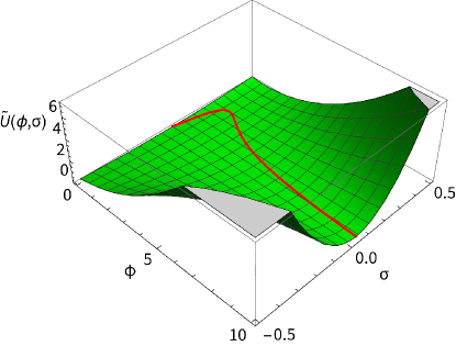
Figure 1: The potential $\tilde{U}(\phi,\,\sigma)$ for $f(\phi)=1+\xi\phi^{2},g(\phi)=\bar{\xi}\phi+\bar{\xi}^{\prime}\phi^{3},V(\phi)=\lambda/4\phi^{4}$, $\beta=10^{6},\delta=\xi=\bar{\xi}=1,\bar{\xi}^{\prime}=0,\lambda=2.3\cdot 10^{-10}$.

where

$$\begin{split}&\mathcal{K}_{1}(\phi,\sigma)=-\frac{1}{2(g^{2}(\phi)\beta+f^{2}(\phi)\delta+4\beta\delta V(\phi))}\Bigg{(}g^{2}(\phi)\hat{\alpha}-2f(\phi)K(\phi)-4g(\phi)((\hat{\alpha}-\hat{\alpha}^{\prime})f(\phi)+\beta K(\phi))\sigma\\ &+4f^{2}(\phi)(\hat{\alpha}-2\hat{\alpha}^{\prime})\sigma^{2}+4(\hat{\alpha}\delta+4(\hat{\alpha}-2\hat{\alpha}^{\prime})\beta\sigma^{2})V(\phi)\Bigg{)}\\ \\ &\mathcal{K}_{2}(\sigma,X)=\frac{24-128(\alpha_{2}X-3)\sigma^{2}}{(1+16\sigma^{2})^{2}},\,\,\,\,\,\,\,\,\mathcal{K}_{3}(\sigma)=\frac{384\sigma^{2}}{(1+16\sigma^{2})^{2}}\\ \\ &\mathcal{K}_{4}(\sigma)=\frac{(-8+\sigma+32\sigma^{2}(-20+\sigma+8\sigma^{2}))\alpha_{2}}{(1+16\sigma^{2})^{2}}=\mathcal{K}_{5}(\sigma)\\ \\ &\tilde{U}(\phi,\sigma)=\left(\frac{f^{2}(\phi)+4\beta V(\phi)}{\delta f^{2}(\phi)+\beta g^{2}(\phi)+4\beta\delta V(\phi)}\right)\left(\sigma-\frac{f(\phi)g(\phi)}{2(f^{2}(\phi)+4\beta V(\phi))}\right)^{2}+\frac{V(\phi)}{f^{2}(\phi)+4\beta V(\phi)}\end{split}{}$$ (4.9)

5 The single-field model

Having in mind to consider the inflationary behavior of the model at hand in the framework of slow-roll inflation, we may neglect acceleration terms as well as terms of higher that two powers of velocities. Doing that, we obtain the following equations of motion for the two scalars

$$\begin{split}&\frac{1}{\sqrt{-g}}\partial_{\mu}\Big{(}\sqrt{-g}\mathcal{K}_{1}(\phi,\sigma)\partial^{\mu}\phi\Big{)}-\frac{1}{2}\frac{\partial\mathcal{K}_{1}(\phi,\sigma)}{\partial\phi}(\nabla_{\mu}\phi)^{2}-\frac{\partial\tilde{U}(\phi,\sigma)}{\partial\phi}=0\\ \\ &\frac{1}{\sqrt{-g}}\partial_{\mu}\Big{(}\sqrt{-g}\mathcal{K}_{2}(\sigma)\partial^{\mu}\sigma\Big{)}-\frac{1}{2}\frac{\partial\mathcal{K}_{2}(\sigma)}{\partial\sigma}(\nabla_{\mu}\sigma)^{2}-\frac{1}{2}\frac{\partial\mathcal{K}_{1}(\phi,\sigma)}{\partial\sigma}(\nabla_{\mu}\phi)^{2}-\frac{\partial\tilde{U}(\phi,\sigma)}{\partial\sigma}=0\end{split}{}$$ (5.1)

The potential of the model, written in the form (4.9), has a manifestly minimum line in the two-field space along the direction

$$\sigma_{0}(\phi)\,=\,\frac{f(\phi)g(\phi)}{2\left(f^{2}(\phi)+4\beta V(\phi)\right)}{}$$ (5.2)

Along this line it reduces to the potential encountered in the Palatini-${\cal{R}}^{2}$ models [71, 73] [102], which is characterized by an inflationary plateau at large values of $V(\phi)$. The potential $\tilde{U}(\phi,\,\sigma)$ and the corresponding minimum valley are shown in Fig 1.

In order to discuss the inflationary behavior of the model at hand we consider an FRW background metric and write the resulting pair of scalar equations. They are

$$\begin{split}&3H\mathcal{K}_{1}(\phi,\sigma)\dot{\phi}+\frac{1}{2}\frac{\partial\mathcal{K}_{1}(\phi,\sigma)}{\partial\phi}\dot{\phi}^{2}+\frac{\partial\mathcal{K}_{1}(\phi,\sigma)}{\partial\sigma}\dot{\phi}\dot{\sigma}+\mathcal{K}_{1}(\phi,\sigma)\ddot{\phi}+\frac{\partial\tilde{U}(\phi,\sigma)}{\partial\phi}=0\\ \\ &\mathcal{K}_{2}(\sigma)\ddot{\sigma}+3H\mathcal{K}_{2}\dot{\sigma}+\frac{1}{2}\frac{\partial\mathcal{K}_{2}(\sigma)}{\partial\sigma}\dot{\sigma}^{2}-\frac{1}{2}\frac{\partial\mathcal{K}_{1}(\phi,\sigma)}{\partial\sigma}\dot{\phi}^{2}+\frac{\partial\tilde{U}(\phi,\sigma)}{\partial\sigma}=0\end{split}$$ (5.3)

The corresponding Friedmann equation is

$$H^{2}=\frac{\rho}{3}\,\,\,\,\,\,\,\,\,\,\,{\textit{with}}\,\,\,\,\,\,\,\,\rho=\frac{1}{2}\mathcal{K}_{1}(\phi,\sigma)\dot{\phi}^{2}+\frac{1}{2}K_{2}(\sigma)\dot{\sigma}^{2}+\tilde{U}(\phi,\sigma)\,.$$ (5.4)

We have solved numerically the coupled system of the equations (5.3) for characteristic values of the parameters and initial conditions $\phi(0)=\sigma(0)=10$ and $\dot{\phi}(0)=\dot{\sigma}(0)=0$. The result is shown in Fig. 2, justifying a rather fast evolution of the two-field system towards the minimum line (5.2). Therefore, we can safely conclude that the system evolves rapidly into a single-field system.

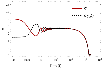
(a)

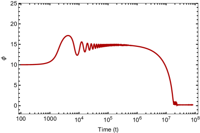
(b)

Figure 2: (a)The pseudoscalar $\sigma$ and (b) the scalar field $\phi$ as functions of time $(t)$, for $f(\phi)=1+\xi\phi^{2}$, $g(\phi)=\bar{\xi}\phi+\bar{\xi}^{\prime}\phi^{3}$, $V(\phi)=\lambda/4\phi^{4}$, $K(\phi)=1$, $\beta=10^{6}$, $\xi=\delta=1=\bar{\xi}^{\prime}=1$, $\bar{\xi}=0$, $\hat{\alpha}=-10^{5},\,\hat{\alpha}^{\prime}=-10^{2}$. This general behavior persists for other values of the parameters aswell.

Inserting the equation of the minimum line (5.2) into the action (4.9) we obtain a single-field action with the potential reduced to just the Palatini-${\cal{R}}^{2}$ term and the kinetic function augmented by the extra contribution of the $\sigma$-kinetic term $(\nabla\sigma_{0})^{2}=(\nabla\phi)^{2}(\sigma_{0}^{\prime}(\phi)\,)^{2}$. We get

$${\cal{S}}=\int\,{\rm d}^{4}x\,\sqrt{-g}\Bigg{\{}\frac{1}{2}R(g)-\frac{1}{2}\bar{\cal{K}}(\phi)(\nabla_{\mu}\phi)^{2}-\bar{U}(\phi)(\phi)\Bigg{\}}\,,{}$$ (5.5)

where

$$\begin{split}&\bar{\mathcal{K}}(\phi)=\bar{\mathcal{K}}_{1}(\phi)+\bar{\mathcal{K}}_{2}(\phi)\Bigg{(}-\frac{(f(\phi)g(\phi))\left(2f(\phi)f^{\prime}(\phi)+4\beta V^{\prime}(\phi)\right)}{2\left(f^{2}(\phi)+4\beta V(\phi)\right)^{2}}\\ &+\frac{g(\phi)f^{\prime}(\phi)}{2\left(f^{2}(\phi)+4\beta V(\phi)\right)}+\frac{f(\phi)g^{\prime}(\phi)}{2\left(f^{2}(\phi)+4\beta V(\phi)\right)}\Bigg{)}^{2}\\ \\ &\bar{\mathcal{K}}_{1}(\phi)=\frac{f(\phi)K(\phi)-2\hat{\alpha}V(\phi)}{f^{2}(\phi)+4\beta V(\phi)}\,,\,\,\,\,\,\,\,\,\,\,\,\bar{\mathcal{K}}_{2}(\phi)=\frac{24\left(f^{2}(\phi)+4\beta V(\phi)\right)^{2}}{4f^{2}(\phi)g^{2}(\phi)+\left(f^{2}(\phi)+4\beta V(\phi)\right)^{2}}\\ \\ &\bar{U}(\phi)=\frac{V(\phi)}{f^{2}(\phi)+4\beta V(\phi)}\end{split}$$ (5.6)

Note that, although there is no trace of the Holst coupling parametric function in the single-field potential, there is a strong dependence on it, as well as on the derivative coupling parameter $\hat{\alpha}$, in the kinetic function $\bar{\cal{K}}(\phi)$.

6 Inflation

We proceed to analyze the inflationary profile of the single-field model assuming the slow-roll approximation. We start with the scalar (${\cal{P}}_{\zeta}$) and tensor (${\cal{P}}_{T}$) power spectra selecting an arbitrary pivot scale $k_{\star}$ that exited the horizon. Their expressions are

$$\mathcal{P}_{\zeta}(k)=A_{s}\left(\frac{k}{k_{\star}}\right)^{n_{s}-1},\,\,\,\,{\textit{where}}\,\,\,\,\,A_{s}\simeq\frac{1}{24\pi^{2}}\frac{\bar{U}(\phi_{\star})}{\epsilon_{\bar{U}}(\phi_{\star})},\,\,\,\,\,\,{\textit{and}}\,\,\,\,\,\,\,\mathcal{P}_{T}(k)\simeq\frac{2\bar{U}(\phi_{\star})}{3\pi^{2}}\left(\frac{k}{k_{\star}}\right)^{n_{t}}\,,$$ (6.1)

$A_{s}$ being the amplitude of the power spectrum of scalar perturbations. The scalar ($n_{s}$) and tensor ($n_{t}$) spectral indices given by

$$n_{s}-1=\frac{{\rm d}\ln\mathcal{P}_{\zeta}(k)}{{\rm d}\ln k}\simeq-6\epsilon_{\bar{U}}+2\eta_{\bar{U}}\qquad\text{and}\qquad n_{t}=\frac{{\rm d}\ln\mathcal{P}_{T}(k)}{{\rm d}\ln k}\,,$$ (6.2)

characterize the scale-dependence of the power spectra (6.1). The tensor-to-scalar ratio is defined as

$$r=\frac{\mathcal{P}_{T}(k)}{\mathcal{P}_{\zeta}(k)}\simeq 16\epsilon_{\bar{U}}.$$ (6.3)

These equations are expressed in terms of the potential slow-roll parameters

$$\epsilon_{\bar{U}}=\frac{1}{2\bar{\mathcal{K}}(\phi)}\left(\frac{\bar{U}^{\prime}(\phi)}{\bar{U}(\phi)}\right)^{2}\qquad\text{and}\qquad\eta_{\bar{U}}=\frac{\left(\bar{\mathcal{K}}^{-1/2}(\phi)\bar{U}^{\prime}(\phi)\right)^{\prime}}{\bar{\mathcal{K}}^{1/2}(\phi)\bar{U}(\phi)}\,.$$ (6.4)

The primes denote derivatives with respect the scalar field, while both slow-roll parameters are assumed to be small $(\ll 1)$ during inflation. The duration of inflation is measured by the number of $e$-folds, given by

$$N_{\star}=\int^{\phi_{\star}}_{\phi_{\rm end}}\bar{\mathcal{K}}(\phi)\frac{\bar{U}(\phi)}{\bar{U}^{\prime}(\phi)}{\rm d}\phi\,,$$ (6.5)

where the end of inflation at $\phi_{end}$ is determined by $\epsilon_{\bar{U}}(\phi_{end})\,\approx\,1\,$. We specify the model taking the scalar field $\phi$ to have a canonical kinetic term ($K(\phi)=1$) and a quartic potential

$N_{\star}$ (e-folds)	$\phi_{\star}$ ($\hat{\alpha}=-10^{3}$)	$\phi_{\star}$ ($\hat{\alpha}=-10^{10}$)
50	19.55	6.15
55	20.54	6.30
60	21.48	6.44
$N_{\star}$ (e-folds)	$\phi_{\star}$ ($\hat{\alpha}=-10^{3}$)	$\phi_{\star}$ ($\hat{\alpha}=-10^{10}$)
50	12.09	5.85
55	12.72	6.01
60	13.33	6.16

Table 1: The first table corresponds to $\xi=1$, $\bar{\xi}=0$, $\bar{\xi}^{\prime}=1$, $\beta=10^{6}$ while the second to $\xi=1$, $\bar{\xi}=1$, $\bar{\xi}^{\prime}=0$, $\beta=10^{6}$.

$$V(\phi)=\frac{\lambda}{4}\phi^{4}\,.$$ (6.6)

The non-minimal coupling functions are taken to be

$$f(\phi)=1+\xi\phi^{2},\quad g(\phi)=\bar{\xi}\phi+\bar{\xi}^{\prime}\phi^{3}\,.$$ (6.7)

The number of e-folds $N_{\star}$ as a function of the initial value of the field $\phi_{\star}$ is obtained by numerical integration of (6.5). Characteristic values are given in table 1 for representative values of the parameters.

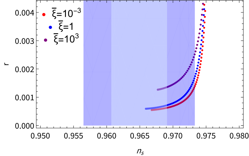
(a)

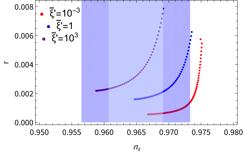
(b)

Figure 3: The spectral index $n_{s}$ with respect to $r$ in order to have $N_{\star}=60$. The parameters we chosen are $\beta=10^{6}$ and $\lambda$ is fixed in order to have $A_{s}\sim 2.1\cdot 10^{-9}$. (a) $\xi=1$, $\bar{\xi}^{\prime}=0$ and $\bar{\xi}=10^{-3}$ (red), $\bar{\xi}=1$ (blue) and $\bar{\xi}=10^{3}$ (purple). (b) $\bar{\xi}^{\prime}=10^{-3}$ (red), $\bar{\xi}^{\prime}=10$ (blue), $\bar{\xi}^{\prime}=10^{3}$ (purple). The lines trace the different values of the derivative coupling parameter $\hat{\alpha}$ with a significant effect on observables for values $10^{2}\leq|{\hat{\alpha}}|\leq 10^{10}$ for which $n_{s}$ increases with $\hat{\alpha}$. We have indicated with light-blue the $1\sigma$ and with dark blue the $2\sigma$ [138, 139].

The existing observations of CMB [138, 139], corresponding to the Planck, BICER/Keck and BAO data, constrain the observables at the pivot scale $k_{\star}=0.05\,{\rm Mpc}^{-1}$ to be

$$A_{s}=(2.10\pm 0.03)\times 10^{-9},\,\,\,n_{s}=0.9649\pm 0.0042\,\,(1\sigma),\,\,\,\,r<0.03$$ (6.8)

In Fig. 3 and 4 we have plotted $n_{s}$ versus $r$ for various choices of the coupling parameters for $N_{\star}\sim 55$ and $N_{\star}\sim 60$. The value of the quartic coupling $\lambda$ is determined from the above $A_{s}$ value. For the representative parameter values of table 1 it has a negligible dependence on $\hat{\alpha}$, as long as $|\hat{\alpha}|<10^{10}$. As we have mentioned above the invertibility of the disformal transformation requires that $\hat{\alpha}<0$. As it can be seen in Fig. 3 the calculated values of the indices $n_{s}$ and $r$ lie for the most part within the acceptable range of observations. Increasing values of $\hat{\alpha}$ lead to an increasing tensor-to-scalar ratio $r$ and tend to push the model values outside the acceptable domain. This is more evident in Fig. 3(a) which corresponds to a linear Holst coupling. As it is more evident in Fig. 3(b), which refers to a cubic Holst coupling, larger values of the corresponding parameter are favored, although they also lead to a faster increase of $r$ with $\hat{\alpha}$. In these cases we found numerically that for $|\hat{\alpha}|\sim 10^{9}$ the scalar tilt becomes $n_{s}\sim 0.9733$. Therefore, for all values of $|\hat{\alpha}|>10^{9}$ the model is pushed outside of the observational data. The known inflationary behavior in the absence of derivative couplings, due to the $R^{2}$ term and /or the $\xi$-coupling is sustained as long as $\hat{\alpha}$ does not exceed certain value, depending on the form and strength of the Holst coupling. We note that in $\hat{\alpha}=0$ limit the values of the observables are in agreement with the previous study [102]. There it was established that that $n_{s}$ and $r$ tend to increase for increasing $\bar{\xi}$ and $\bar{\xi}^{\prime}$. This feature remains also true in the present case as it can be seen in the corresponding figures.

(a)

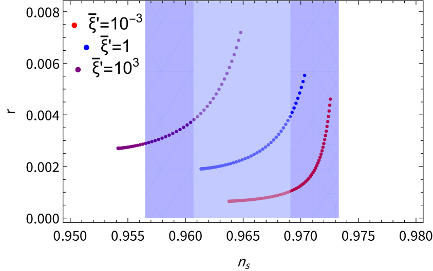
(b)

Figure 4: The spectral index $n_{s}$ with respect to $r$ in order to have $N_{\star}=55$. The parameters we chosen are $\beta=10^{6}$ and $\lambda$ is fixed in order to have $A_{s}\sim 2.1\cdot 10^{-9}$. (a) $\xi=1$, $\bar{\xi}^{\prime}=0$ and $\bar{\xi}=10^{-3}$ (red), $\bar{\xi}=1$ (blue) and $\bar{\xi}=10^{3}$ (purple). (b) $\xi=1$ and $\bar{\xi}=0$, $\bar{\xi}^{\prime}=10^{-3}$ (red), $\bar{\xi}^{\prime}=1$ (blue), $\bar{\xi}^{\prime}=10^{3}$ (purple). The lines trace the different values of the derivative coupling parameter $\hat{\alpha}$ with a significant effect on observables for values $10^{2}\leq|{\hat{\alpha}}|\leq 10^{10}$ for which $n_{s}$ increases with $\hat{\alpha}$. We have indicated with light-blue the $1\sigma$ and with dark blue the $2\sigma$ [138, 139].

In the large $\phi$ limit the kinetic function is of the form $\bar{K}(\phi)\approx|\hat{\alpha}|\lambda/2\left(\beta\lambda+\xi^{2}\right)$. Then, the corresponding canonical field $\phi_{c}=\int\,d\phi\sqrt{K(\phi)}$ is $\phi_{c}\approx\,\phi\left(\frac{|\hat{\alpha}|\lambda}{2(\beta\lambda+\xi^{2})}\right)^{1/2}$, which can easily lie in the subplanckian regime for the representative values of parameters adopted above.

7 Summary

In the present article we have considered the framework of Einstein-Cartan gravity and studied a model of a non-minimally coupled scalar with a quartic $\phi^{4}$ potential that includes up to quadratic terms of the Ricci scalar and the Holst invariant. The found that the model is characterized by an extra dynamical pseudoscalar degree of freedom $\sigma$, associated with the presence of the Holst term. We have analyzed the evolution of the two-field system in an FRW background and found that it evolves rapidly along a trajectory of minimal potential, being reduced into an effective single-field system. We proceeded to study slow-roll inflation for the single-field system, analyzing the effect of the derivative couplings on its inflationary behavior. We focused on the determination of the observables $n_{s}$ and $r$ for representative values of the model parameters and studied their dependence on the derivative coupling parameter $\hat{\alpha}$, finding that an increase in $\alpha$ results in an increase of their corresponding values. We find that the model is cosistent with the latest combined observational data from Planck, BICEP/Keck and BAO for relativelly wide range of its parameters. Nevertheless, for large derivative coupling parameter values $|\hat{\alpha}|>10^{9}$, the model becomes incosistent with observations. It should be noted that the ${\cal{R}}^{2}$ and/or the non-minimal $\xi$-coupling are central to the consistent inflationary behavior of $\phi^{4}$, which is sustained as long as the derivative coupling stays below these values.

Appendix A Appendix

The algebraic solution to the equations of the torsion vectors, in terms of $E_{\mu}$, given in (3.13), is

$$\begin{split}&\hat{T}_{\mu}=\frac{1}{A}E_{\mu}-\frac{B}{A(A+BX)}X_{\mu\nu}E^{\nu}\\ \\ &T_{\mu}=\frac{1}{A}\Big{(}F_{4}+\frac{1}{6}F_{5}X\Big{)}E_{\mu}+\Bigg{\{}\frac{1}{3A}F_{5}-\frac{B}{A(A+BX)}\Big{(}F_{4}+\frac{1}{6}F_{5}X\Big{)}-\frac{1}{3}F_{5}\frac{BX}{A(A+BX)}\Bigg{\}}X_{\mu\nu}E^{\nu}\end{split}$$ (A.1)

where

$$A=\frac{1}{16}+\Big{(}F_{4}+\frac{1}{6}F_{5}X\Big{)}^{2}\,\,\,\,{\text{and}}\,\,\,\,B=\frac{1}{3}\Big{\{}2F_{5}\Big{(}F_{4}+\frac{1}{6}F_{5}X\Big{)}+\frac{1}{3}F_{5}^{2}X\Big{\}}$$ (A.2)

Substituting back into the action (3.11) we obtain

$$\begin{split}\mathcal{S}&=\int{\rm d}^{4}x\sqrt{-g}\Bigg{\{}\frac{1}{2}R-\frac{\Delta^{2}}{3}\Big{[}F^{2}E^{2}+H(2F+HX)(E\cdot X\cdot E)\Big{]}+\frac{\Delta^{2}}{48}\Big{[}E^{2}\\ &+G(GX+2)(E\cdot X\cdot E)\Big{]}+\frac{2}{3}F_{4}\Delta^{2}\Big{[}FE^{2}+(FG+H+HGX)(E\cdot X\cdot E)\Big{]}\\ &+\Delta\Big{[}E\cdot\nabla F_{4}+GE\cdot X\cdot\nabla F_{4})\Big{]}+\frac{\Delta}{3}\Big{[}E\cdot\nabla(F_{5}X)+G(E\cdot X\cdot\nabla(F_{5}X))\Big{]}\\ &-\frac{\Delta}{3}\Big{[}\nabla_{\mu}(\tensor{X}{{}^{\mu}_{\nu}}F_{5})E^{\nu}+G\nabla_{\mu}(\tensor{X}{{}^{\mu}_{\nu}}F_{5})\tensor{X}{{}^{\nu}_{\rho}}E^{\rho}\Big{]}+\frac{2}{9}\Delta^{2}F_{5}\Big{[}(F+FGX\\ &+HX+HGX^{2})(E\cdot X\cdot E)\Big{]}+\frac{\Delta^{2}}{9}F_{5}X\Big{[}FE^{2}+(FG+HGX+H)(E\cdot X\cdot E)\Big{]}\\ &-\frac{1}{2}\gamma_{1}(1+\gamma X)^{-1/2}K(\phi)X-\gamma_{1}^{2}(1+\gamma X)^{1/2}U\Bigg{\}}\end{split}{}$$ (A.3)

expressed in terms of the functions

$$\Delta=A^{-1},\,\,\,F=F_{4}+\frac{1}{6}F_{5}X,\,\,\,G=-\frac{B}{A+BX}\,,\,\,\,\,H=\frac{1}{3}F_{5}+G\Big{(}F+\frac{1}{3}F_{5}X\Big{)}$$ (A.4)

In order to simplify notation, from now on we shall denote $F_{4}=\sigma$. Then, $F_{5}=\gamma F_{4}=\gamma\sigma$. The scalar field action in (A.3) consists of two parts, namely a part

$$\begin{split}\mathcal{S}_{I}&=\int{\rm d}^{4}x\sqrt{-g}\Bigg{\{}-\frac{\Delta^{2}}{3}\Big{[}F^{2}E^{2}+H(2F+HX)(E\cdot X\cdot E)\Big{]}+\frac{\Delta^{2}}{48}\Big{[}E^{2}\\ &+G(GX+2)(E\cdot X\cdot E)\Big{]}+\frac{2}{3}\sigma\Delta^{2}\Big{[}FE^{2}+(FG+H+HGX)(E\cdot X\cdot E)\Big{]}\\ &+\Delta\Big{[}E\cdot\nabla\sigma+GE\cdot X\cdot\nabla\sigma)\Big{]}+\frac{\Delta}{3}\Big{[}E\cdot\nabla(F_{5}X)+G(E\cdot X\cdot\nabla(\gamma\sigma X))\Big{]}\\ &-\frac{\Delta}{3}\Big{[}\nabla_{\mu}(\tensor{X}{{}^{\mu}_{\nu}}\gamma\sigma)E^{\nu}+G\nabla_{\mu}(\tensor{X}{{}^{\mu}_{\nu}}\gamma\sigma)\tensor{X}{{}^{\nu}_{\rho}}E^{\rho}\Big{]}+\frac{2}{9}\Delta^{2}\gamma\sigma\Big{[}(F+FGX\\ &+HX+HGX^{2})(E\cdot X\cdot E)\Big{]}+\frac{\Delta^{2}}{9}\gamma\sigma X\Big{[}FE^{2}+(FG+HGX+H)(E\cdot X\cdot E)\Big{]}\Bigg{\}}\end{split}{}$$ (A.5)

and a part

$${\cal{S}}_{II}=\int\,{\rm d}^{4}x\,\sqrt{-g}\Bigg{\{}-\frac{1}{2}\gamma_{1}(1+\gamma X)^{-1/2}K(\phi)X-\gamma_{1}^{2}(1+\gamma X)^{1/2}U\Bigg{\}}{}$$ (A.6)

${\cal{S}}_{I}$ contains only kinetic terms. To $\mathcal{O}(X)$ it is a function of $\sigma$, its derivative and derivatives of $\phi$, namely

$$\begin{split}\mathcal{S}_{I}&=\int\,{\rm d}^{4}x\,\sqrt{-g}\Bigg{\{}\frac{-12+64(\alpha_{2}X-3)\sigma^{2}}{(1+16\sigma^{2})^{2}}(\nabla_{\mu}\sigma)^{2}-\frac{384\sigma^{2}}{(1+16\sigma^{2})^{2}}X^{\mu\nu}\nabla_{\mu}\sigma\nabla_{\nu}\sigma\\ &+\frac{(-8+\sigma+32\sigma^{2}(-20+\sigma+8\sigma^{2}))\alpha_{2}}{(1+16\sigma^{2})^{2}}\Big{(}\nabla_{\mu}\sigma\nabla^{\mu}(\sigma X)-\nabla_{\mu}(X^{\mu\nu}\sigma)\nabla_{\nu}\sigma\Big{)}\,\,\Bigg{\}}\end{split}$$ (A.7)

The part ${\cal{S}}_{II}$ is a function of all the scalars, including the auxiliary $\chi$.

References

- [1] A. Palatini, Deduzione invariantiva delle equazioni gravitazionali dal principio di hamilton, Rendiconti del Circolo Matematico di Palermo (1884-1940) 43 (Dec, 1919) 203–212.
- [2] F. W. Hehl, J. D. McCrea, E. W. Mielke, and Y. Ne’eman, Metric affine gauge theory of gravity: Field equations, Noether identities, world spinors, and breaking of dilation invariance, Phys. Rept. 258 (1995) 1–171, [gr-qc/9402012].
- [3] F. L. Bezrukov and M. Shaposhnikov, The Standard Model Higgs boson as the inflaton, Phys. Lett. B 659 (2008) 703–706, [arXiv:0710.3755].
- [4] F. Bauer and D. A. Demir, Inflation with Non-Minimal Coupling: Metric versus Palatini Formulations, Phys. Lett. B665 (2008) 222–226, [arXiv:0803.2664].
- [5] S. Rasanen and P. Wahlman, Higgs inflation with loop corrections in the Palatini formulation, JCAP 11 (2017) 047, [arXiv:1709.07853].
- [6] T. Tenkanen, Resurrecting Quadratic Inflation with a non-minimal coupling to gravity, JCAP 12 (2017) 001, [arXiv:1710.02758].
- [7] A. Racioppi, Coleman-Weinberg linear inflation: metric vs. Palatini formulation, JCAP 12 (2017) 041, [arXiv:1710.04853].
- [8] T. Markkanen, T. Tenkanen, V. Vaskonen, and H. Veermäe, Quantum corrections to quartic inflation with a non-minimal coupling: metric vs. Palatini, JCAP 03 (2018) 029, [arXiv:1712.04874].
- [9] L. Järv, A. Racioppi, and T. Tenkanen, Palatini side of inflationary attractors, Phys. Rev. D 97 (2018), no. 8 083513, [arXiv:1712.08471].
- [10] C. Fu, P. Wu, and H. Yu, Inflationary dynamics and preheating of the nonminimally coupled inflaton field in the metric and Palatini formalisms, Phys. Rev. D 96 (2017), no. 10 103542, [arXiv:1801.04089].
- [11] A. Racioppi, New universal attractor in nonminimally coupled gravity: Linear inflation, Phys. Rev. D 97 (2018), no. 12 123514, [arXiv:1801.08810].
- [12] A. Kozak and A. Borowiec, Palatini frames in scalar–tensor theories of gravity, Eur. Phys. J. C 79 (2019), no. 4 335, [arXiv:1808.05598].
- [13] S. Rasanen, Higgs inflation in the Palatini formulation with kinetic terms for the metric, Open J. Astrophys. 2 (2019), no. 1 1, [arXiv:1811.09514].
- [14] J. P. B. Almeida, N. Bernal, J. Rubio, and T. Tenkanen, Hidden Inflaton Dark Matter, JCAP 03 (2019) 012, [arXiv:1811.09640].
- [15] K. Shimada, K. Aoki, and K.-i. Maeda, Metric-affine Gravity and Inflation, Phys. Rev. D 99 (2019), no. 10 104020, [arXiv:1812.03420].
- [16] T. Takahashi and T. Tenkanen, Towards distinguishing variants of non-minimal inflation, JCAP 04 (2019) 035, [arXiv:1812.08492].
- [17] R. Jinno, K. Kaneta, K.-y. Oda, and S. C. Park, Hillclimbing inflation in metric and Palatini formulations, Phys. Lett. B 791 (2019) 396–402, [arXiv:1812.11077].
- [18] J. Rubio and E. S. Tomberg, Preheating in Palatini Higgs inflation, JCAP 1904 (2019), no. 04 021, [arXiv:1902.10148].
- [19] A. Racioppi, Non-Minimal (Self-)Running Inflation: Metric vs. Palatini Formulation, JHEP 21 (2020) 011, [arXiv:1912.10038].
- [20] M. Shaposhnikov, A. Shkerin, and S. Zell, Quantum Effects in Palatini Higgs Inflation, JCAP 07 (2020) 064, [arXiv:2002.07105].
- [21] A. Borowiec and A. Kozak, New class of hybrid metric-Palatini scalar-tensor theories of gravity, JCAP 07 (2020) 003, [arXiv:2003.02741].
- [22] L. Järv, A. Karam, A. Kozak, A. Lykkas, A. Racioppi, and M. Saal, Equivalence of inflationary models between the metric and Palatini formulation of scalar-tensor theories, Phys. Rev. D 102 (2020), no. 4 044029, [arXiv:2005.14571].
- [23] A. Karam, M. Raidal, and E. Tomberg, Gravitational dark matter production in Palatini preheating, JCAP 03 (2021) 064, [arXiv:2007.03484].
- [24] J. McDonald, Does Palatini Higgs Inflation Conserve Unitarity?, JCAP 04 (2021) 069, [arXiv:2007.04111].
- [25] M. Langvik, J.-M. Ojanperä, S. Raatikainen, and S. Rasanen, Higgs inflation with the Holst and the Nieh–Yan term, Phys. Rev. D 103 (2021), no. 8 083514, [arXiv:2007.12595].
- [26] M. Shaposhnikov, A. Shkerin, I. Timiryasov, and S. Zell, Higgs inflation in Einstein-Cartan gravity, JCAP 02 (2021) 008, [arXiv:2007.14978]. [Erratum: JCAP 10, E01 (2021)].
- [27] M. Shaposhnikov, A. Shkerin, I. Timiryasov, and S. Zell, Einstein-Cartan gravity, matter, and scale-invariant generalization, JHEP 10 (2020) 177, [arXiv:2007.16158].
- [28] Y. Mikura, Y. Tada, and S. Yokoyama, Conformal inflation in the metric-affine geometry, EPL 132 (2020), no. 3 39001, [arXiv:2008.00628].
- [29] S. Verner, Quintessential Inflation in Palatini Gravity, JCAP 04 (2021) [arXiv:2010.11201].
- [30] V.-M. Enckell, S. Nurmi, S. Räsänen, and E. Tomberg, Critical point Higgs inflation in the Palatini formulation, JHEP 04 (2021) 059, [arXiv:2012.03660].
- [31] Y. Reyimuaji and X. Zhang, Natural inflation with a nonminimal coupling to gravity, JCAP 03 (2021) 059, [arXiv:2012.14248].
- [32] A. Karam, S. Karamitsos, and M. Saal, -function reconstruction of Palatini inflationary attractors, JCAP 10 (2021) 068, [arXiv:2103.01182].
- [33] Y. Mikura, Y. Tada, and S. Yokoyama, Minimal -inflation in light of the conformal metric-affine geometry, Phys. Rev. D 103 (2021), no. 10 L101303, [arXiv:2103.13045].
- [34] A. Racioppi, J. Rajasalu, and K. Selke, Multiple point criticality principle and Coleman-Weinberg inflation, JHEP 06 (2022) 107, [arXiv:2109.03238].
- [35] Y. Mikura and Y. Tada, On UV-completion of Palatini-Higgs inflation, JCAP 05 (2022), no. 05 035, [arXiv:2110.03925].
- [36] D. Y. Cheong, S. M. Lee, and S. C. Park, Reheating in models with non-minimal coupling in metric and Palatini formalisms, JCAP 02 (2022), no. 02 029, [arXiv:2111.00825].
- [37] H. Azri, I. Bamwidhi, and S. Nasri, Isocurvature modes and non-Gaussianity in affine inflation, Phys. Rev. D 104 (2021), no. 10 104064, [arXiv:2111.03828].
- [38] A. Racioppi and M. Vasar, On the number of e-folds in the Jordan and Einstein frames, Eur. Phys. J. Plus 137 (2022), no. 5 637, [arXiv:2111.09677].
- [39] M. Piani and J. Rubio, Higgs-Dilaton inflation in Einstein-Cartan gravity, JCAP 05 (2022), no. 05 009, [arXiv:2202.04665].
- [40] G. K. Karananas, M. Shaposhnikov, and S. Zell, Field redefinitions, perturbative unitarity and Higgs inflation, JHEP 06 (2022) 132, [arXiv:2203.09534].
- [41] C. Rigouzzo and S. Zell, Coupling metric-affine gravity to a Higgs-like scalar field, Phys. Rev. D 106 (2022), no. 2 024015, [arXiv:2204.03003].
- [42] I. D. Gialamas, A. Karam, and T. D. Pappas, Gravitational corrections to electroweak vacuum decay: metric vs. Palatini, Phys. Lett. B 840 (2023) 137885, [arXiv:2212.03052].
- [43] S. C. Hyun, J. Kim, T. Kodama, S. C. Park, and T. Takahashi, Nonminimally assisted inflation: a general analysis, JCAP 05 (2023) 050, [arXiv:2302.05866].
- [44] M. Piani and J. Rubio, Preheating in Einstein-Cartan Higgs Inflation: oscillon formation, JCAP 12 (2023) 002, [arXiv:2304.13056].
- [45] I. D. Gialamas and H. Veermäe, Electroweak vacuum decay in metric-affine gravity, Phys. Lett. B 844 (2023) 138109, [arXiv:2305.07693].
- [46] C. Rigouzzo and S. Zell, Coupling metric-affine gravity to the standard model and dark matter fermions, Phys. Rev. D 108 (2023), no. 12 124067, [arXiv:2306.13134].
- [47] B. Barman, N. Bernal, and J. Rubio, Rescuing Gravitational-Reheating in Chaotic Inflation, arXiv:2310.06039.
- [48] L. Amendola, Cosmology with nonminimal derivative couplings, Phys. Lett. B 301 (1993) 175–182, [gr-qc/9302010].
- [49] S. Capozziello and G. Lambiase, Nonminimal derivative coupling and the recovering of cosmological constant, Gen. Rel. Grav. 31 (1999) 1005–1014, [gr-qc/9901051].
- [50] S. Capozziello, G. Lambiase, and H. J. Schmidt, Nonminimal derivative couplings and inflation in generalized theories of gravity, Annalen Phys. 9 (2000) 39–48, [gr-qc/9906051].
- [51] C. Germani and A. Kehagias, New Model of Inflation with Non-minimal Derivative Coupling of Standard Model Higgs Boson to Gravity, Phys. Rev. Lett. 105 (2010) 011302, [arXiv:1003.2635].
- [52] S. Tsujikawa, Observational tests of inflation with a field derivative coupling to gravity, Phys. Rev. D 85 (2012) 083518, [arXiv:1201.5926].
- [53] K. Kamada, T. Kobayashi, T. Takahashi, M. Yamaguchi, and J. Yokoyama, Generalized Higgs inflation, Phys. Rev. D 86 (2012) 023504, [arXiv:1203.4059].
- [54] H. M. Sadjadi and P. Goodarzi, Reheating in nonminimal derivative coupling model, JCAP 02 (2013) 038, [arXiv:1203.1580].
- [55] G. Koutsoumbas, K. Ntrekis, and E. Papantonopoulos, Gravitational Particle Production in Gravity Theories with Non-minimal Derivative Couplings, JCAP 08 (2013) 027, [arXiv:1305.5741].
- [56] Y. Ema, R. Jinno, K. Mukaida, and K. Nakayama, Particle Production after Inflation with Non-minimal Derivative Coupling to Gravity, JCAP 10 (2015) 020, [arXiv:1504.07119].
- [57] B. Gumjudpai and P. Rangdee, Non-minimal derivative coupling gravity in cosmology, Gen. Rel. Grav. 47 (2015), no. 11 140, [arXiv:1511.00491].
- [58] Y. Zhu and Y. Gong, PPN parameters in gravitational theory with nonminimally derivative coupling, Int. J. Mod. Phys. D 26 (2016), no. 02 1750005, [arXiv:1512.05555].
- [59] H. Sheikhahmadi, E. N. Saridakis, A. Aghamohammadi, and K. Saaidi, Hamilton-Jacobi formalism for inflation with non-minimal derivative coupling, JCAP 10 (2016) 021, [arXiv:1603.03883].
- [60] I. Dalianis, G. Koutsoumbas, K. Ntrekis, and E. Papantonopoulos, Reheating predictions in Gravity Theories with Derivative Coupling, JCAP 02 (2017) 027, [arXiv:1608.04543].
- [61] T. Harko, F. S. N. Lobo, E. N. Saridakis, and M. Tsoukalas, Cosmological models in modified gravity theories with extended nonminimal derivative couplings, Phys. Rev. D 95 (2017), no. 4 044019, [arXiv:1609.01503].
- [62] G. Tumurtushaa, Inflation with Derivative Self-interaction and Coupling to Gravity, Eur. Phys. J. C 79 (2019), no. 11 920, [arXiv:1903.05354].
- [63] C. Fu, P. Wu, and H. Yu, Primordial Black Holes from Inflation with Nonminimal Derivative Coupling, Phys. Rev. D 100 (2019), no. 6 063532, [arXiv:1907.05042].
- [64] I. Dalianis, S. Karydas, and E. Papantonopoulos, Generalized Non-Minimal Derivative Coupling: Application to Inflation and Primordial Black Hole Production, JCAP 06 (2020) 040, [arXiv:1910.00622].
- [65] S. Sato and K.-i. Maeda, Stability of hybrid Higgs inflation, Phys. Rev. D 101 (2020), no. 10 103520, [arXiv:2001.00154].
- [66] S. Karydas, E. Papantonopoulos, and E. N. Saridakis, Successful Higgs inflation from combined nonminimal and derivative couplings, Phys. Rev. D 104 (2021), no. 2 023530, [arXiv:2102.08450].
- [67] A. A. Starobinsky, A New Type of Isotropic Cosmological Models Without Singularity, Phys. Lett. B 91 (1980) 99–102.
- [68] X.-H. Meng and P. Wang, corrections to the cosmological dynamics of inflation in the Palatini formulation, Class. Quant. Grav. 21 (2004) 2029–2036, [gr-qc/0402011].
- [69] M. Borunda, B. Janssen, and M. Bastero-Gil, Palatini versus metric formulation in higher curvature gravity, JCAP 11 (2008) 008, [arXiv:0804.4440].
- [70] F. Bombacigno and G. Montani, Big bounce cosmology for Palatini gravity with a Nieh–Yan term, Eur. Phys. J. C 79 (2019), no. 5 405, [arXiv:1809.07563].
- [71] V.-M. Enckell, K. Enqvist, S. Rasanen, and L.-P. Wahlman, Inflation with term in the Palatini formalism, JCAP 02 (2019) 022, [arXiv:1810.05536].
- [72] D. Iosifidis, A. C. Petkou, and C. G. Tsagas, Torsion/non-metricity duality in f(R) gravity, Gen. Rel. Grav. 51 (2019), no. 5 66, [arXiv:1810.06602].
- [73] I. Antoniadis, A. Karam, A. Lykkas, and K. Tamvakis, Palatini inflation in models with an term, JCAP 11 (2018) 028, [arXiv:1810.10418].
- [74] I. Antoniadis, A. Karam, A. Lykkas, T. Pappas, and K. Tamvakis, Rescuing Quartic and Natural Inflation in the Palatini Formalism, JCAP 03 (2019) 005, [arXiv:1812.00847].
- [75] T. Tenkanen, Minimal Higgs inflation with an term in Palatini gravity, Phys. Rev. D 99 (2019), no. 6 063528, [arXiv:1901.01794].
- [76] A. Edery and Y. Nakayama, Palatini formulation of pure gravity yields Einstein gravity with no massless scalar, Phys. Rev. D 99 (2019), no. 12 124018, [arXiv:1902.07876].
- [77] M. Giovannini, Post-inflationary phases stiffer than radiation and Palatini formulation, Class. Quant. Grav. 36 (2019), no. 23 235017, [arXiv:1905.06182].
- [78] I. D. Gialamas and A. Lahanas, Reheating in Palatini inflationary models, Phys. Rev. D 101 (2020), no. 8 084007, [arXiv:1911.11513].
- [79] A. Lloyd-Stubbs and J. McDonald, Sub-Planckian inflation in the Palatini formulation of gravity with an term, Phys. Rev. D 101 (2020), no. 12 123515, [arXiv:2002.08324].
- [80] I. Antoniadis, A. Lykkas, and K. Tamvakis, Constant-roll in the Palatini- models, JCAP 04 (2020), no. 04 033, [arXiv:2002.12681].
- [81] D. M. Ghilencea, Palatini quadratic gravity: spontaneous breaking of gauged scale symmetry and inflation, Eur. Phys. J. C 80 (4, 2020) 1147, [arXiv:2003.08516].
- [82] N. Das and S. Panda, Inflation and Reheating in f(R,h) theory formulated in the Palatini formalism, JCAP 05 (2021) 019, [arXiv:2005.14054].
- [83] I. D. Gialamas, A. Karam, and A. Racioppi, Dynamically induced Planck scale and inflation in the Palatini formulation, JCAP 11 (2020) 014, [arXiv:2006.09124].
- [84] D. M. Ghilencea, Gauging scale symmetry and inflation: Weyl versus Palatini gravity, Eur. Phys. J. C 81 (2021), no. 6 510, [arXiv:2007.14733].
- [85] D. Iosifidis and L. Ravera, Parity Violating Metric-Affine Gravity Theories, Class. Quant. Grav. 38 (2021), no. 11 115003, [arXiv:2009.03328].
- [86] S. Bekov, K. Myrzakulov, R. Myrzakulov, and D. S.-C. Gómez, General slow-roll inflation in gravity under the Palatini approach, Symmetry 12 (2020), no. 12 1958, [arXiv:2010.12360].
- [87] K. Dimopoulos and S. Sánchez López, Quintessential inflation in Palatini gravity, Phys. Rev. D 103 (2021), no. 4 043533, [arXiv:2012.06831].
- [88] A. Karam, E. Tomberg, and H. Veermäe, Tachyonic preheating in Palatini inflation, JCAP 06 (2021) 023, [arXiv:2102.02712].
- [89] A. Lykkas and K. Tamvakis, Extended interactions in the Palatini- inflation, JCAP 08 (2021), no. 043 [arXiv:2103.10136].
- [90] I. D. Gialamas, A. Karam, T. D. Pappas, and V. C. Spanos, Scale-invariant quadratic gravity and inflation in the Palatini formalism, Phys. Rev. D 104 (2021), no. 2 023521, [arXiv:2104.04550].
- [91] I. Antoniadis, A. Guillen, and K. Tamvakis, Ultraviolet behaviour of Higgs inflation models, JHEP 08 (2021) 018, [arXiv:2106.09390]. [Addendum: JHEP 05, 074 (2022)].
- [92] I. D. Gialamas, A. Karam, T. D. Pappas, A. Racioppi, and V. C. Spanos, Scale-invariance, dynamically induced Planck scale and inflation in the Palatini formulation, J. Phys. Conf. Ser. 2105 (2021), no. 1 012005, [arXiv:2107.04408].
- [93] M. AlHallak, A. AlRakik, N. Chamoun, and M. S. El-Daher, Palatini f(R) Gravity and Variants of k-/Constant Roll/Warm Inflation within Variation of Strong Coupling Scenario, Universe 8 (2022), no. 2 126, [arXiv:2111.05075].
- [94] C. Dioguardi, A. Racioppi, and E. Tomberg, Slow-roll inflation in Palatini F(R) gravity, JHEP 06 (2022) 106, [arXiv:2112.12149].
- [95] K. Dimopoulos, A. Karam, S. Sánchez López, and E. Tomberg, Modelling Quintessential Inflation in Palatini-Modified Gravity, Galaxies 10 (2022), no. 2 57, [arXiv:2203.05424].
- [96] K. Dimopoulos, A. Karam, S. Sánchez López, and E. Tomberg, Palatini R 2 quintessential inflation, JCAP 10 (2022) 076, [arXiv:2206.14117].
- [97] G. Pradisi and A. Salvio, (In)equivalence of metric-affine and metric effective field theories, Eur. Phys. J. C 82 (2022), no. 9 840, [arXiv:2206.15041].
- [98] R. Durrer, O. Sobol, and S. Vilchinskii, Magnetogenesis in Higgs-Starobinsky inflation, Phys. Rev. D 106 (2022), no. 12 123520, [arXiv:2207.05030].
- [99] A. Salvio, Inflating and reheating the Universe with an independent affine connection, Phys. Rev. D 106 (2022), no. 10 103510, [arXiv:2207.08830].
- [100] I. Antoniadis, A. Guillen, and K. Tamvakis, Late time acceleration in Palatini gravity, JHEP 11 (2022) 144, [arXiv:2207.13732].
- [101] A. B. Lahanas, Issues in Palatini inflation: Bounds on the reheating temperature, Phys. Rev. D 106 (2022), no. 12 123530, [arXiv:2210.00837].
- [102] I. D. Gialamas and K. Tamvakis, Inflation in metric-affine quadratic gravity, JCAP 03 (2023) 042, [arXiv:2212.09896].
- [103] C. Dioguardi, A. Racioppi, and E. Tomberg, Inflation in Palatini quadratic gravity (and beyond), arXiv:2212.11869.
- [104] D. Iosifidis, R. Myrzakulov, and L. Ravera, Cosmology of Metric-Affine R+ Gravity with Pure Shear Hypermomentum, Fortsch. Phys. 72 (2024), no. 1 2300003, [arXiv:2301.00669].
- [105] I. D. Gialamas and K. Tamvakis, Bimetric-affine quadratic gravity, Phys. Rev. D 107 (2023), no. 10 104012, [arXiv:2303.11353].
- [106] I. D. Gialamas, A. Karam, T. D. Pappas, and E. Tomberg, Implications of Palatini gravity for inflation and beyond, arXiv:2303.14148.
- [107] S. Sánchez López, K. Dimopoulos, A. Karam, and E. Tomberg, Observable gravitational waves from hyperkination in Palatini gravity and beyond, Eur. Phys. J. C 83 (2023), no. 12 1152, [arXiv:2305.01399].
- [108] C. Dioguardi and A. Racioppi, Palatini : a new framework for inflationary attractors, arXiv:2307.02963.
- [109] A. Di Marco, E. Orazi, and G. Pradisi, Einstein–Cartan pseudoscalaron inflation, Eur. Phys. J. C 84 (2024), no. 2 146, [arXiv:2309.11345].
- [110] D. A. Gomes, R. Briffa, A. Kozak, J. Levi Said, M. Saal, and A. Wojnar, Cosmological constraints of Palatini f(R) gravity, JCAP 01 (2024) 011, [arXiv:2310.17339].
- [111] W.-Y. Hu, Q.-Y. Wang, Y.-Q. Ma, and Y. Tang, Gravitational Waves from Preheating in Inflation with Weyl Symmetry, arXiv:2311.00239.
- [112] I. D. Gialamas and K. Tamvakis, Inflation in Weyl-invariant Einstein-Cartan gravity, Phys. Rev. D 111 (2025), no. 4 044007, [arXiv:2410.16364].
- [113] I. D. Gialamas, T. Katsoulas, and K. Tamvakis, Inflation and reheating in quadratic metric-affine gravity with derivative couplings, JCAP 06 (2024) 005, [arXiv:2403.08530].
- [114] I. D. Gialamas and A. Racioppi, Symmetry-breaking inflation in non-minimal metric-affine gravity, arXiv:2412.17738.
- [115] D. Kazanas, Dynamics of the Universe and Spontaneous Symmetry Breaking, Astrophys. J. Lett. 241 (1980) L59–L63.
- [116] K. Sato, First Order Phase Transition of a Vacuum and Expansion of the Universe, Mon. Not. Roy. Astron. Soc. 195 (1981) 467–479.
- [117] A. H. Guth, The Inflationary Universe: A Possible Solution to the Horizon and Flatness Problems, Phys. Rev. D 23 (1981) 347–356.
- [118] A. D. Linde, A New Inflationary Universe Scenario: A Possible Solution of the Horizon, Flatness, Homogeneity, Isotropy and Primordial Monopole Problems, Phys. Lett. B 108 (1982) 389–393.
- [119] A. A. Starobinsky, Spectrum of relict gravitational radiation and the early state of the universe, JETP Lett. 30 (1979) 682–685.
- [120] V. F. Mukhanov and G. V. Chibisov, Quantum Fluctuations and a Nonsingular Universe, JETP Lett. 33 (1981) 532–535.
- [121] S. W. Hawking, The Development of Irregularities in a Single Bubble Inflationary Universe, Phys. Lett. B 115 (1982) 295.
- [122] A. A. Starobinsky, Dynamics of Phase Transition in the New Inflationary Universe Scenario and Generation of Perturbations, Phys. Lett. B 117 (1982) 175–178.
- [123] A. H. Guth and S. Y. Pi, Fluctuations in the New Inflationary Universe, Phys. Rev. Lett. 49 (1982) 1110–1113.
- [124] J. M. Bardeen, P. J. Steinhardt, and M. S. Turner, Spontaneous Creation of Almost Scale - Free Density Perturbations in an Inflationary Universe, Phys. Rev. D 28 (1983) 679.
- [125] E. Cartan, Sur les variétés à connexion affine et la théorie de la relativité généralisée. (première partie), Annales Sci. Ecole Norm. Sup. 40 (1923) 325–412.
- [126] E. Cartan, Sur les variétés à connexion affine et la théorie de la relativité généralisée. (première partie) (Suite)., Annales Sci. Ecole Norm. Sup. 41 (1924) 1–25.
- [127] I. D. Gialamas, A. Karam, A. Lykkas, and T. D. Pappas, Palatini-Higgs inflation with nonminimal derivative coupling, Phys. Rev. D 102 (2020), no. 6 063522, [arXiv:2008.06371].
- [128] H. B. Nezhad and S. Rasanen, Scalar fields with derivative coupling to curvature in the Palatini and the metric formulation, JCAP 02 (2024) 009, [arXiv:2307.04618].
- [129] J. Beltrán Jiménez and A. Delhom, Ghosts in metric-affine higher order curvature gravity, Eur. Phys. J. C 79 (2019), no. 8 656, [arXiv:1901.08988].
- [130] J. Beltrán Jiménez and A. Delhom, Instabilities in metric-affine theories of gravity with higher order curvature terms, Eur. Phys. J. C 80 (2020), no. 6 585, [arXiv:2004.11357].
- [131] C. Marzo, Radiatively stable ghost and tachyon freedom in metric affine gravity, Phys. Rev. D 106 (2022), no. 2 024045, [arXiv:2110.14788].
- [132] J. Annala and S. Rasanen, Stability of non-degenerate Ricci-type Palatini theories, JCAP 04 (2023) 014, [arXiv:2212.09820]. [Erratum: JCAP 08, E02 (2023)].
- [133] W. Barker and C. Marzo, Particle spectra of general Ricci-type Palatini or metric-affine theories, arXiv:2402.07641.
- [134] W. Barker and S. Zell, Consistent particle physics in metric-affine gravity from extended projective symmetry, arXiv:2402.14917.
- [135] Y. N. Obukhov, E. J. Vlachynsky, W. Esser, R. Tresguerres, and F. W. Hehl, An Exact solution of the metric affine gauge theory with dilation, shear, and spin charges, Phys. Lett. A 220 (1996) 1, [gr-qc/9604027].
- [136] Y. N. Obukhov, E. J. Vlachynsky, W. Esser, and F. W. Hehl, Irreducible decompositions in metric affine gravity models, gr-qc/9705039.
- [137] W. Barker, C. Marzo, and C. Rigouzzo, PSALTer: Particle Spectrum for Any Tensor Lagrangian, arXiv:2406.09500.
- [138] Planck Collaboration, Y. Akrami et al., Planck 2018 results. X. Constraints on inflation, Astron. Astrophys. 641 (2020) A10, [arXiv:1807.06211].
- [139] BICEP, Keck Collaboration, P. A. R. Ade et al., Improved Constraints on Primordial Gravitational Waves using Planck, WMAP, and BICEP/Keck Observations through the 2018 Observing Season, Phys. Rev. Lett. 127 (2021), no. 15 151301, [arXiv:2110.00483].