Convergence of Shallow ReLU Networks
on Weakly Interacting Data

Abstract

We analyse the convergence of one-hidden-layer ReLU networks trained by gradient flow on $n$ data points. Our main contribution leverages the high dimensionality of the ambient space, which implies low correlation of the input samples, to demonstrate that a network with width of order $\log(n)$ neurons suffices for global convergence with high probability. Our analysis uses a Polyak–Łojasiewicz viewpoint along the gradient-flow trajectory, which provides an exponential rate of convergence of $\frac{1}{n}$. When the data are exactly orthogonal, we give further refined characterizations of the convergence speed, proving its asymptotic behavior lies between the orders $\frac{1}{n}$ and $\frac{1}{\sqrt{n}}$, and exhibiting a phase-transition phenomenon in the convergence rate, during which it evolves from the lower bound to the upper, and in a relative time of order $\frac{1}{\log(n)}$.

1 Introduction

Understanding the properties of models used in machine learning is crucial for providing guarantees to downstream users. Of particular importance, the convergence of the training process under gradient methods stands as one of the first issues to address in order to comprehend them. If, on the one hand, such a question for linear models and convex optimization problems [Bottou et al., 2018, Bach, 2024] are well understood, this is not the case for neural networks, which are the most used models in large-scale machine learning. This paper focuses on providing quantitative convergence guarantees for a one-hidden-layer neural network.

Theoretically, such global convergence analysis of neural networks has seen two main achievements in the past years: (i) the identification of the lazy regime, due to a particular initialization, where convergence is always guaranteed at the cost of being essentially a linear model [Jacot et al., 2018, Arora et al., 2019, Chizat et al., 2019], and (ii) the proof that with an infinite amount of hidden units a two-layer neural network converges towards the global minimizer of the loss [Mei et al., 2018, Chizat and Bach, 2018, Rotskoff and Vanden-Eijnden, 2018]. However, neural networks are trained in practice outside of these regimes, as neural networks are known to perform feature learning, and experimentally reach global minimum with a large but finite number of neurons. Quantifying in which regimes neural networks converge to a global minimum of their loss is still an important open question.

This article aims to identify such a regime, characterized by low-correlated inputs, under which we can rigorously prove the convergence of shallow neural networks trained via gradient flow. The previous assumptions needed for convergence relied on special initialization scales [Chizat et al., 2019, Boursier et al., 2022], on an infinite number of neurons [Jacot et al., 2018, Chizat and Bach, 2018], or on the exact orthogonality of the input data [Boursier et al., 2022, Frei et al., 2023]. In this article, we aim to simply fix the dimension $d$, and ask how many randomly sampled examples can be interpolated by the network with high probability. This high dimensionality regime, corresponding to $d$ being larger than $n^{2}$, is our main assumption to prove convergence of shallow ReLU neural networks. In addition, we are interested in understanding the general dynamics of the system, and in particular the system’s convergence speed to a global minimizer of the loss.

We summarize our contributions in the analysis of the learning dynamics of a one-hidden-layer ReLU network on a finite number of data $n$ via gradient flow.

• Our main contribution is that shallow neural networks in high dimension $d\geq Cn^{2}$ interpolates exactly random whitened data with high probability as soon as the neural network has more that $\log(n)$ neurons, for any initialization scale. We also show that the loss converges to zero exponentially fast with a rate at least of order $\frac{1}{n}$.

• Then, when the inputs are orthogonal, we refine our analysis in order to characterize the range of possible asymptotic speeds, which we find to be at most of order $\frac{1}{\sqrt{n}}$. Moreover, we conjecture that this speed is always of the highest order $\frac{1}{\sqrt{n}}$ with high probability and verify empirically this claim.

• Finally, for orthonormal inputs and a special initialization of the network, we highlight a phase transition in the convergence rate during the system’s evolution, and compute the associated cut-off time and transition period.

2 Problem Setup

Notations.

We use $||v||$ to denote the euclidean norm of a vector $v$, $\langle\cdot|\cdot\rangle$ its scalar product, and $||M||$ for the operator norm associated with $||\cdot||$ of a matrix $M$. Moreover, let $\bar{v}=\frac{v}{||v||}$.

Loss function.

Let $(x_{i},y_{i})_{i=1:n}\in(\mathbb{R}^{d}\times\mathbb{R})^{n}$ be a sample of input vectors and real outputs. Let $d\in\mathbb{N}^{*}$ be the dimension of the vector space and $n\in\mathbb{N}^{*}$ the number of data points. In order to learn the regression problem of mapping $x_{i}$ to $y_{i}$, we use one-hidden-layer ReLU neural networks, which we write:

$$h_{\theta}(x)=\frac{1}{p}\sum_{j=1}^{p}a_{j}\sigma(\langle w_{j}|x\rangle)\,,$$ (1)

where $p\in\mathbb{N}^{*}$ is the number of units, $\sigma(x)=\max\{0,x\}$ for $x\in\mathbb{R}$ is the rectified linear unit (ReLU), and the parameters are gathered in $\theta=(a_{j},w_{j})_{1\leq j\leq p}\in(\mathbb{R}\times\mathbb{R}^{d})^{p}$. To simplify the ReLU notation, we define $\sigma(\langle w_{j}|x_{i}\rangle)=\langle w_{j}|x_{i}\rangle_{+}$ and $\mathbb{1}_{\langle w_{j}|x_{i}\rangle>0}=1_{j,i}$. When mentioning neurons of the network, we refer to $\langle w_{j}|x_{i}\rangle_{+}$, while second layer neurons refer to $a_{j}$. Neurons can be activated if $\langle w_{j}|x_{i}\rangle_{+}>0$, and are correctly activated if moreover $a_{j}y_{i}>0$. Upon this prediction class and data, we analyse the regression loss with square error,

$$L(\theta):=\frac{1}{2n}\sum_{i=1}^{n}(y_{i}-h_{\theta}(x_{i}))^{2}\leavevmode\nobreak\ .$$ (2)

As soon as $d\geq n$, ${(x_{i})_{i=1:n}}$ can form a free family, in which case the set of minima of $L$, which consists of all interpolators, is non-empty.

Gradient flow.

In order to understand a simplified version of the optimization dynamics of this neural network, we study the continuous-time limit of gradient descent. We initialize $\theta_{t=0}=\theta_{0}$ and follow for all $t\geq 0$ the ordinary differential equation

$$\frac{d}{dt}\theta_{t}=-p\nabla_{\theta_{t}}L(\theta_{t})\,,$$ (3)

where we choose a particular element of the sub-differential of the ReLU $\sigma^{\prime}(x)=\mathbb{1}_{x>0}$, for any $x\in\mathbb{R}$. This choice is motivated by both prior empirical work from Bertoin et al. [2021] and theoretical work from Boursier et al. [2022, Proposition 2] and Jentzen and Riekert [2023]. We also decided to accelerate the dynamics by a factor $p$ as only this scaling gives a consistent mean field limit for the gradient flow when the number of neurons tends to infinity (see Definition 2.2 by Chizat and Bach [2018]).

Weight invariance.

The 1-homogeneity of the ReLU provides a continuous symmetry in the function $\theta\mapsto h_{\theta}$ and hence the loss. This feature is known to lead automatically to invariants in the gradient flow as explained generally by Marcotte et al. [2024]. The following lemma is not new [Wojtowytsch, 2020, p.11], and shows that, from this invariance, we deduce that the two layers have balanced contributions throughout the dynamics.

Lemma 1.

For all $j\in\llbracket 1,p\rrbracket$, for all $t\geq 0$, $|a_{j}(t)|^{2}-||w_{j}(t)||^{2}=|a_{j}(0)|^{2}-||w_{j}(0)||^{2}$ , and thus, if $|a_{j}(0)|\geq||w_{j}(0)||$, then $a_{j}(t)$ maintains its sign and $|a_{j}(t)|\geq||w_{j}(t)||$.

Initialization.

Throughout the paper, we initialize the network’s weights $w_{j}$ and $a_{j}$ from a joint distribution where both marginals are non-zero, centered, rotational-invariant, have finite covariance, and we take norms of $a_{j}$ and $w_{j}$ independent of $d,n,p$. Moreover, we need an assumption of asymmetry of the norm at initialization.

Assumption 1 (Asymmetric norm initialization).

We assume that the weights of the network at initialization satisfy $\forall j\in\llbracket 1,p\rrbracket,\ |a_{j}(0)|\geq||w_{j}(0)||$.

Articles by Boursier and Flammarion [2024a, b] already used this assumption to study two-layer neural networks in order to use the property described in Lemma 1.

Data.

We define the data matrix $X=(x_{1},\ldots,x_{n})\in\mathbb{R}^{d\times n}$. Denote $C_{x}^{-}=\min_{i}||x_{i}||$ and $C_{y}^{-}=\min_{i}|y_{i}|$; in what follows, we suppose that $C_{x}^{-}>0$ and $C_{y}^{-}>0$, i.e., the input and output data are bounded away from the origin. Similarly, we also let $C_{x}^{+}=\max_{i}||x_{i}||$ and $C_{y}^{+}=\max_{i}|y_{i}|$. We note $C_{x,y}^{+,-}$ to refer to the set of these constants. Finally, we introduce the following hypothesis on the low correlation between the inputs.

Assumption 2 (Low correlated inputs).

We assume that the data satisfy

$$||X^{T}X-D_{X}||<\frac{(C_{x}^{-})^{2}}{\sqrt{n}}\frac{C_{y}^{-}}{C_{y}^{+}}\leavevmode\nobreak\ ,$$ (4)

where $D_{X}$ denotes the diagonal matrix with coefficients $||x_{i}||^{2}$.

The term $||X^{T}X-D_{X}||$ is a control on the magnitude of the correlations $(\langle x_{i},x_{j}\rangle)_{i\neq j}$. As an extreme case, when it equals zero, the inputs are orthogonal. This assumption is purely deterministic at this stage. Later, we show that this weak interaction between the inputs is highly likely to occur for random whitened vectors in high dimensions (see Corollary 1).

Dimensions.

Throughout the paper, even if the results provided are all non-asymptotic in nature, the reader can picture that the numbers $n,p,d$ (respectively data, neurons and dimension) are all large. Moreover, they verify the following constraint: $n$ is less than $d$, and $p$ can be thought of the order $\log(n)$, meaning only a “low” number of neurons is required.

2.1 Related works

Convergence of neural networks.

Neural networks are known to converge under specific data, parameter, or initialization hypotheses, among which: the neural tangent kernel regime studied by Jacot et al. [2018], Arora et al. [2019], Du et al. [2019], Allen-Zhu et al. [2019], that has been shown to correspond in fact to a lazy regime where there is no feature learning because of the initialization scale. Another field of study is the mean-field regime, where feature learning can happen but where the optimization has been shown to converge only in the infinite width case [Mei et al., 2018, Chizat and Bach, 2018, Rotskoff and Vanden-Eijnden, 2018]. Note that it is also possible to produce generic counter examples, where convergence does not occur [Boursier and Flammarion, 2024b]. Beyond these, there have been attempts to generalize convergence results under local PL (or local curvature) conditions as shown by Chatterjee [2022], Liu et al. [2022], Zhou et al. [2021], but they remain unsatisfactory to explain the good general behavior of neural networks due to the constraint it imposes on the initialization. Convergence theorems similar in spirit to Theorem 1 can be found in an article by Chen et al. [2022]. The main difference relies on two features: only the inner weights are trained and their result necessitates a large value of outer weights when $n$ is large, which is the regime of interest of the present article. Finally, it is worth mentioning other works on neural networks dynamics, e.g., the study of the implicit bias either for regression [Boursier et al., 2022] or classification [Lyu and Li, 2020, Ji and Telgarsky, 2020], or sample complexity to learn functions in a specific context [Glasgow, 2023].

Polyak-Łojasiewicz properties.

Dating back from the early sixties, Polyak derived a sufficient criterion for a smooth gradient descent to converge to a global minimizer [Polyak, 1964]. This corresponds to the later-called Polyak-Łojasiewicz (PL) constant $\mu$ of a function $f:\mathbb{R}^{d}\rightarrow\mathbb{R}_{+}$, that can be defined as the best exponential rate of convergence of gradient flow over all initializations, or equivalently to the following minimum ratio $\mu=\min_{x\in\mathbb{R}^{d}}\frac{||\nabla f(x)||^{2}}{f(x)}$. This has found many applications in non-convex optimization, as it is the case for neural network optimization, and is very popular for optimization in the space of measures [Gentil, 2020]. Other notions of PL conditions have emerged in the literature to characterize local convergence, by bounding the PL constant over a ball $\mu^{*}(z,r)=\min_{x\in\mathcal{B}(z,r)}\frac{||\nabla f(x)||^{2}}{f(x)}$ [Chatterjee, 2022, Liu et al., 2022] and comparing it to $f(z)$. We use a notion of PL which is local and trajectory-wise to prove lower bounds valid on each trajectory.

3 Convergence in high dimension

In this first section, our goal is to understand when the gradient flow converges toward a global minimizer of the loss. Note that the parametrization of the prediction function $h_{\theta}$ by a neural network often implies the non-convexity of the objective $L$ and prevents any direct application of convex tools in order to ensure global convergence. Generally speaking, even if gradient flows are expected to converge to critical points of the parameter space [Lee et al., 2016], such that $\nabla_{\theta}L(\theta)=0$, they might become stuck in local minimizers that do not interpolate the data.

3.1 Local PL-curvature

Convexity is not the only tool that provides global convergence: as known in the optimization community, showing that $\frac{||\nabla L(\theta)||^{2}}{L(\theta)}$ is uniformly lower bounded suffices. As mentioned in Section 2.1, this is known as the Polyak-Lojasiewicz condition [Polyak, 1964]. Taking a dynamical perspective on this, we define a trajectory-wise notion of this “curvature” condition which we name the local-PL curvature of the system, and define for all $t\geq 0$,

$$\mu(t):=p\frac{\|\nabla L(\theta_{t})\|^{2}}{L(\theta_{t})}=-\frac{\frac{d}{dt}L(\theta_{t})}{L(\theta_{t})}$$ (5)

with the second equality being a property of the gradient flow. Intuitively, this coefficient describes the curvature in parameter space that $\theta_{t}$ “sees” at time $t\geq 0$. The following lemma is classical and shows how it can be used to prove the global convergence of the system, as well as a quantification on the rate.

Lemma 2.

Let $\langle\mu(t)\rangle:=\frac{1}{t}\int_{0}^{t}\mu(u)du$ the time average of the local-PL curvature, which we name the average-PL curvature. We have L$(\theta_{t})=L(\theta(0))e^{-\langle\mu(t)\rangle t}$.

Hence, if the total average-PL curvature $\langle\mu_{\infty}\rangle:=\lim_{t\to\infty}\langle\mu(t)\rangle$ is strictly positive, we can deduce an upper bound on the loss and convergence to $0$ at the exponential speed $\langle\mu_{\infty}\rangle$. This shows that the average-PL curvature is actually the instantaneous exponential decay rate of the loss, and thus controls the speed at which the system converges.

3.2 Global convergence of neural networks for weakly correlated inputs

We are ready to state the main theorem of the paper on the minimization of the loss.

Theorem 1.

Let $\varepsilon>0$, $p\geq 4\log(\frac{n}{\varepsilon})$, and suppose Assumption 1. We fix the data $(x_{i},y_{i})_{1\leq i\leq n}$ and suppose it satisfies Assumption 2. Then with probability at least $1-\varepsilon$ over the initialization of the network, the loss converges to 0 with $\langle\mu_{\infty}\rangle\geq\frac{C}{n}$, where we define $C=\frac{(C_{x}^{-})^{2}}{C_{x}^{+}}C_{y}^{-}$. Moreover, for any $t\geq 0$, we have the lower bound

$$\begin{split}\mu(t)&\geq\frac{C}{n}\min_{i}\left|1-\frac{r_{i}(t)}{y_{i}}\right|.\end{split}$$ (6)

Note that, at best, the number of neurons required in Theorem 1 is logarithmic. This finiteness stands in contrast with the infinite number required in the mean-field regime, and the polynomial dependency typical of the neural tangent kernel (NTK) regime [Jacot et al., 2018, Allen-Zhu et al., 2019]. In the orthogonal case, the ReLU makes the $\log(n)$ dependency necessary and sufficient, as shown in Lemma 5, as the residual $r_{i}$ goes to zero if and only if a neuron gets initialized as $a_{j}y_{i}>0$ and $\langle w_{j}|x_{i}\rangle>0$ for each $i$.

Assumption 2 is crucial for this proof: it means that the examples are insufficiently correlated with each other for the weights to collapse onto a single direction. As proved by Boursier and Flammarion [2024a, Theorem 1], the direction $\bar{w}^{*}=\arg\min_{\theta=\{\bar{w},a\}}L(\theta)$ will attract all neurons if it is accessible from anywhere on the initialization landscape. This phenomenon known as early alignment and first described by Maennel et al. [2018], will prevent interpolation if examples are highly correlated [Boursier and Flammarion, 2024a, Theorem 2]. The fact that our result holds for any initialization scale shows that near-orthogonal inputs prevent accessibility to $\bar{w}^{*}$ and make the early alignment phenomenon benign, as found by Boursier et al. [2022], Frei et al. [2023].

Note finally that our norm-asymmetric initialization (Assumption 1) is sufficient for global convergence with high probability, but may not be necessary. That said, we present in Appendix C.1 a detailed example of interpolation failure when the assumption is not satisfied.

Convergence in high dimension.

In this paragraph we assume that the data $(x_{i},y_{i})_{i=1:n}$ are generated i.i.d. from some distribution $\mathcal{P}_{X,Y}$. We first show that, with high probability, Assumption 2 is almost always valid if the dimension is larger than the square root of the number of data points. Additionally, we assume that the law anti-concentrates at the origin. These two features are gathered in the following lemma.

Lemma 3.

Let $(x_{i},y_{i})_{1\leq i\leq n}$ be generated i.i.d. from a probability distribution $\mathcal{P}_{X,Y}$ such that the marginal $\mathcal{P}_{X}$ is sub-Gaussian, has zero-mean, and satisfy $\mathbb{E}_{x\sim\mathcal{P}_{X}}[xx^{T}]=\frac{\lambda^{2}}{d}I_{d}$ for some $\lambda$ independent of $d,n$, while, on $\mathbb{R}^{*}$, the marginal law $\mathcal{P}_{Y}$ has compact support. There exists $C>0$ depending only on the constants $C_{x,y}^{+,-}$ and the initialization weights, such that, if $d\geq C\left(n^{2}+n\log\left(\frac{1}{\varepsilon}\right)\right)$, then, with probability $1-\varepsilon$, Assumption 2 is satisfied.

The hypothesis in the previous lemma is satisfied by standard distributions like Gaussians $\mathcal{N}(0,\frac{1}{d}I_{d})$ for the inputs. The following corollary restates Theorem 1 for data that are generically distributed as in Lemma 3, and when the dimension is large enough.

Corollary 1.

Let $\varepsilon>0$. Suppose Assumption 1 and that $(x_{i},y_{i})_{1\leq i\leq n}$ are i.i.d. generated from a probability distribution satisfying the same properties as in Lemma 3. There exists a constant $C>0$ depending only on the constants $C_{x,y}^{+,-}$ such that, if the network has $p\geq 8\log\left(\frac{n}{\varepsilon}\right)$ neurons in dimension $d\geq C\left(n^{2}+n\log\left(\frac{1}{\varepsilon}\right)\right)$, then, with probability at least $1-\varepsilon$ over the initialization of the network and the data generation, the loss converges to 0 at exponential speed of rate at least $\frac{1}{n}$.

Beyond the high-dimensionality of the inputs, Corollary 1 does not require any initialization specificity (small or large), and the number of neurons required to converge can be as low as $\log(n)$. Hence, let us put emphasis on the fact that the global nice structure of the loss landscape comes from the high-dimensionality: this does not come from a specific region in which the network is initialized as in the NTK (or lazy) regime [Chatterjee, 2022], nor rely on the infinite number of neurons [Wojtowytsch, 2020].

Remark that, under the near-orthogonality assumption, in the large $d$ limit, the largest amount of data that “fits” in the vector space is only $d$, and corresponds to a perturbation of the canonical basis. On average, Corollary 1 finally states that the average number of data points for which we can show convergence is of the order $\sqrt{d}$. Trying to push back this limit up to order $d$ is an important question for future research and seems to ask for other techniques. Experiments underlying this question are presented in Section 5 (Figure 2).

3.3 Sketch of Proof

The proof of convergence relies on three key points: (i) the loss strictly decreases as long as each example is activated by at least a neuron, (ii) for a data point, if there exists a neuron which is activated at initialization, then at least one neuron remains activated throughout the dynamics, (iii) At initialization, condition (ii) is satisfied with large probability. Let us detail shortly how each item articulates with one another.

(i).

First, Lemma 6, stated and proved in Appendix, shows that, by computing the derivatives of the loss, we get a lower bound on the curvature

$$\mu(t)\geq\frac{2}{n}((C_{x}^{-})^{2}-||X^{T}X-D_{X}||)\min_{i}\left\{\frac{1}{p}\sum_{j=1}^{p}|a_{j}|^{2}1_{j,i}\right\}.$$ (7)

To prove the strict positivity, one needs to show that $||X^{T}X-D_{X}||$ is small enough, and that for each data $i$, there exists $j$ such that $|a_{j}|^{2}1_{j,i}$ is strictly positive. Thanks to the initialization of the weights, $|a_{j}|^{2}\geq|a_{j}(0)|^{2}-||w_{j}(0)||^{2}>0$, and to Assumption 2, $\frac{1}{\sqrt{2}}(C_{x}^{-})^{2}>||X^{T}X-D_{X}||$. Thus, we have convergence if at any time, for any data input, one neuron remains active, i.e., formally, for all $t\geq 0$, and all $i\in\llbracket 1,n\rrbracket$, there exists $j\in\llbracket 1,p\rrbracket$ such that $\langle w_{j}(t)|x_{i}\rangle_{+}>0$. Hence, the loss decreases as long as one neuron remains active per data input. We see next how to show this crucial property.

(ii).

Let us fix the data index $i\in\llbracket 1,n\rrbracket$, and $y_{i}>0$ without loss of generality. Let us define $j^{*}_{i}\leavevmode\nobreak\ =\leavevmode\nobreak\ \arg\max_{a_{j}y_{i}>0}\langle w_{j}(t)|x_{i}\rangle$ the index of the largest correctly initialized neuron. Since $a_{j}$ cannot change sign thanks to Assumption 1, $\langle w_{j_{i}^{*}}(t)|x_{i}\rangle$ is continuous, and has a derivative over each constant segment of $j_{i}^{*}$. The strict positivity of this neuron is an invariant of the dynamics: if $r_{i}\geq y_{i}$, the derivative of the neuron shows it increases, and if $r_{i}<y_{i}$, the residual has decreased, which implies that the $\langle w_{j_{i}^{*}}(t)|x_{i}\rangle$ is strictly positive. Thus, if a neuron is correctly initialized for the data point $i$, a neuron stays active throughout the dynamics.

(iii).

Finally, Lemma 5 shows $\mathbb{P}(\forall i,\exists j,\langle w_{j}(0)|x_{i}\rangle>0\cap a_{j}y_{i}>0)\geq 1-n\left(\frac{3}{4}\right)^{p}$, which implies that for $p\geq 4\log(\frac{n}{\varepsilon})$, the network is well initialized with probability at least $1-\varepsilon$.

4 Orthogonal Data

In this section, we go deeper on the study of the gradient flow, assuming that the input data are perfectly orthogonal, or equivalently that $||X^{T}X-D_{X}||=0$. Since most of the intuition for the convergence is drawn from the orthogonal case, it offers stronger results which we detail. In particular, we are able to closely understand the local-PL curvature $(\mu(t))_{t\geq 0}$ evolution and asymptotic behaviour.

4.1 Asymptotic PL curvature

Theorem 1 has shown that the local-PL curvature is lower bounded by a term of order $\frac{1}{n}$, allowing us to show an exponential convergence rate of this order. The following proposition shows that in the orthogonal case the curvature can also be upper bounded.

Proposition 1.

Let $\varepsilon>0$. Given orthogonal inputs, Assumption 1, $d$ large enough, and $p\geq 4\log(\frac{n}{\varepsilon})$, with probability $1-\varepsilon$, we have an upper-bound on the local-PL curvature: there exists $C>0$ depending only on the initialization and the constants $C_{x,y}^{+,-}$ such that for all $t\geq Cn$,

$$\mu(t)\leq C\sqrt{\frac{p}{n}}\max_{i}\left|1-\frac{r_{i}(t)}{y_{i}}\right|+\frac{C}{n}.\\$$ (8)

This upper bound uses two properties that are characteristic of the orthogonal case. First, once a neuron is inactive on some data input, then, it can never re-activate again. The second property is that for an initialization scale independent on $n$, there is a phase during which correctly initialized neurons increase while the others decrease to 0. This extinction phase, proved in Lemma 7, is short in comparison to the time needed to fit the residuals, and leaves the system decoupled between positive and negative outputs $y_{i}$.

In the limit where $n$ goes to infinity, Proposition 1 shows that the network does not learn since the local-PL is 0. This is an artifact of the orthogonality of the inputs: the interaction between inputs should accelerate the dynamics. However, although all quantities have well defined limits as $n\rightarrow+\infty$, the limits cannot be understood as a gradient descent in an infinite dimensional space.

Proposition 1 is in fact valid for $p$ fixed, and an initialization of the weights for which every data is correctly initialized by a neuron. In that case, Proposition 1 shows that the asymptotic curvature cannot be larger than the order $\frac{1}{\sqrt{n}}$. While the local-PL curvature is between the order $\frac{1}{n}$ and $\frac{1}{\sqrt{n}}$, the next proposition shows that any intermediate order $\frac{1}{n^{\alpha}}$, for $\alpha\in[\frac{1}{2},1]$, can be reached asymptotically, with strictly positive probability, using a particular initialization of the network.

Group initialization.

In the following, we use $p_{n}$ to denote the number of neurons, and partition the $n$ data points in $p_{n}$ groups of cardinality $k_{n}$ (note that $p_{n}k_{n}=n$). We re-index the examples per group as by $(x_{i}^{j},y_{i}^{j})=(x_{i+(j-1)k_{n}},y_{i+(j-1)k_{n}})$, for all $i\in\llbracket 1,k_{n}\rrbracket$ and $j\in\llbracket 1,p_{n}\rrbracket$. Moreover, we use a special initialization of the network such that for all $j,q\in\llbracket 1,p_{n}\rrbracket$, $i\in\llbracket 1,k_{n}\rrbracket$,

$$\bigg{\{}\begin{matrix}\langle w_{j}|x_{i}^{q}\rangle>0\text{ if }j=q\\ \langle w_{j}|x_{i}^{q}\rangle\leq 0\text{ if }j\neq q\\ \end{matrix}\ \ \text{ and }\ \ a_{j}=s_{j}||w_{j}||\leavevmode\nobreak\ ,$$ (9)

i.e., $w_{j}$ is correctly activated on the group $j$ only.

Proposition 2.

Suppose the group initialization described above, with orthonormal inputs, i.e., $X^{T}X=I$, and that the signs of all outputs of the group $j$ are equal to $s_{j}$. We fix $k_{n}=n^{2(1-\alpha)}$ with $\alpha\in[\frac{1}{2},1]$. Then, for $t\geq Cn^{3\alpha-1}\log\left(Cn\right)$, the local-PL curvature satisfies

$$\frac{K_{1}}{n^{\alpha}}\leq\mu(t)\leq\frac{K_{2}}{n^{\alpha}},$$ (10)

where $C=\max(\alpha C_{y}^{-},(\frac{1}{2C_{y}^{-}})^{\frac{1}{\alpha}})$, $K_{1}=2C_{y}^{-}\min_{j}\frac{||w_{j}(0)||^{2}}{2+||w_{j}(0)||^{2}}$ and $K_{2}=4C_{y}^{+}$.

Proposition 2 states that any asymptotic value $\langle\mu_{\infty}\rangle\in[\frac{K_{1}}{n},\frac{K_{2}}{\sqrt{n}}]$ can be achieved with strictly positive probability using group initialization. But of what order is the most likely limit of the curvature for standard initialization? Experiment 5.2 in Section 5.2 suggest that, with high probability, the asymptotic curvature is always of the order $\frac{1}{\sqrt{n}}$.

Conjecture 1.

Let $\varepsilon>0$. There exist $C_{1},C_{2}>0$ depending only on the data and the initialization, such that for $p\geq C_{1}\log(\frac{n}{\varepsilon})$ and for orthogonal examples, with probability at least $1-\varepsilon$ over the initialization of the network, we have convergence of the loss to 0 and

$$\langle\mu_{\infty}\rangle=\frac{C_{2}}{\sqrt{n}}.$$ (11)

4.2 Phase transition in the PL curvature

In the previous section, we emphasized the asymptotic order of the local-PL curvature with respect to $n$ and hypothesized that it is of the order $\frac{1}{\sqrt{n}}$ in most cases. In this section, we are interested in the evolution of the local-PL curvature during the dynamics. Lemma 4 below computes the local-PL curvature at initialization in the large $p$ regime, and shows that initially it is of order $\frac{1}{n}$.

Lemma 4.

At initialization, the local-PL curvature $\mu(0)$ is a random variable which satisfy $\sqrt{p}(\frac{2}{n}\mu(0)-\beta_{0})\underset{p\rightarrow+\infty}{\longrightarrow}\mathcal{N}\left(0,\gamma_{0}^{2}\right)$, and with $\beta_{0},\gamma_{0}$ depending only on the data and the distributions of the network’s neurons.

The constant $\beta_{0}$ is strictly positive as soon as the limit network does not directly equal the labels, which is natural to assume since they are unknown a priori. Thus the exponential rate of decrease of the loss in the early times of the dynamics is of order $\frac{1}{n}$. Importantly, Proposition 2 with a single group has an asymptotic speed of order $\frac{1}{\sqrt{n}}$, meaning that the local-PL curvature transitions between $\frac{1}{n}$ and $\frac{1}{\sqrt{n}}$. If Conjecture 1 is true, then this phenomenon happens with high probability during the dynamics.

Let us study this phenomenon through the example of Proposition 2, with a fixed number of neurons $p$. In this case, the following theorem shows that there are exactly $p$ phase transitions of the loss, which each corresponds to a data group being fitted. To be precise, let us define $L_{\infty}(t)=\lim_{n\rightarrow+\infty}L_{n}(t)$, with $L_{n}(t)=L(\theta(t\times{t_{n}}))$, $t_{n}=\frac{\sqrt{np}}{4}\log(np)$, and $p$ fixed ($k_{n}=\frac{n}{p}$). We prove that $L_{\infty}$ is constant by parts with at most $p$ parts.

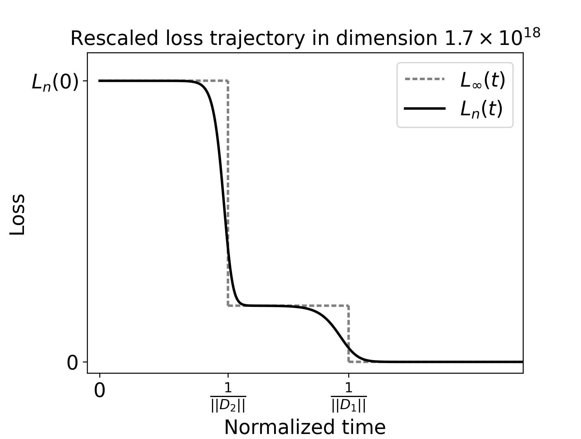
Figure 1: Simulation of the loss trajectory of a network with 2 neurons and group initialization, each activated separately on half the data points. $L_{n}$ is the rescaled loss for $n$ examples, and $L_{\infty}$ is its limit as $n$ goes to infinity. We can see two phase transitions in the very high-dimensional regime.

Theorem 2.

Suppose the same data hypothesis and initialization as Proposition 2. We define $||D_{j}^{n}||^{2}=\frac{1}{k_{n}}\sum_{i=1}^{k_{n}}(y_{i}^{j})^{2}$ for each cluster, and suppose its limit $||D_{j}^{\infty}||^{2}$ finite. Then, the function $L_{\infty}$ is constant by parts with at most $p$ parts, and the transitions happen at each time $t^{j}=\frac{1}{||D_{j}^{\infty}||}$. Moreover, for all $\varepsilon\in]0,1[$, there exist times $t_{n}^{j}({\varepsilon})$ satisfying

$$L^{j}(t_{n}^{j}({\varepsilon}))=\frac{\varepsilon}{2}||D_{j}^{n}||^{2},\,\,\frac{t_{n}^{j}({\varepsilon})}{t_{n}^{j}(1-{\varepsilon})}\sim_{n}1\text{ and }\frac{t_{n}^{j}(1-{\varepsilon})-t_{n}^{j}({\varepsilon})}{t_{n}}\sim_{n}\frac{1}{2||D_{j}^{\infty}||}\frac{\log\left(C^{j}(\varepsilon)\right)}{\log(n)},$$ (12)

where $L^{j}$ is the part of the loss corresponding to the group $j$, and $C^{j}(\varepsilon)>1$ depends on $\varepsilon$ and the initializations and data of the group $j$.

The theorem shows that each transition of $L_{n}$ occurs in the time frame which decreases as $\frac{1}{\log(n)}$. Note that these transitions are subtle: one needs extremely large dimensions in order to differentiate two close transitions as shown on Figure 1 in Appendix. The phase transitions of the loss are in fact associated with transitions $||w_{j}||^{2}$ from a constant order to an order $\sqrt{n}$, and by Lemma 6 with transitions on the local-PL from order $\frac{1}{n}$ to order $\frac{1}{\sqrt{n}}$.

5 Experiments

In this Section, we aim to perform deeper experimental investigations on the system, which we could not do formally. Precisely, we want to answer two questions:

1. What is the probability that the loss reaches 0 for $n$ data points in dimension $d$, under the distributional hypotheses of Lemma 3 (sub-Gaussian, zero-mean and whitened data)? What is the maximum $n$ for a fixed $d$ such that global convergence holds with high probability ?

2. In the orthogonal case, is the asymptotic exponential convergence rate of order $\frac{1}{\sqrt{n}}$ (on average over the initialization) as stated in Conjecture 1?

The data and weights distribution which have been used for the experiments below can be found in Appendix B, and the code is available on GitHub.

5.1 Probability of Convergence

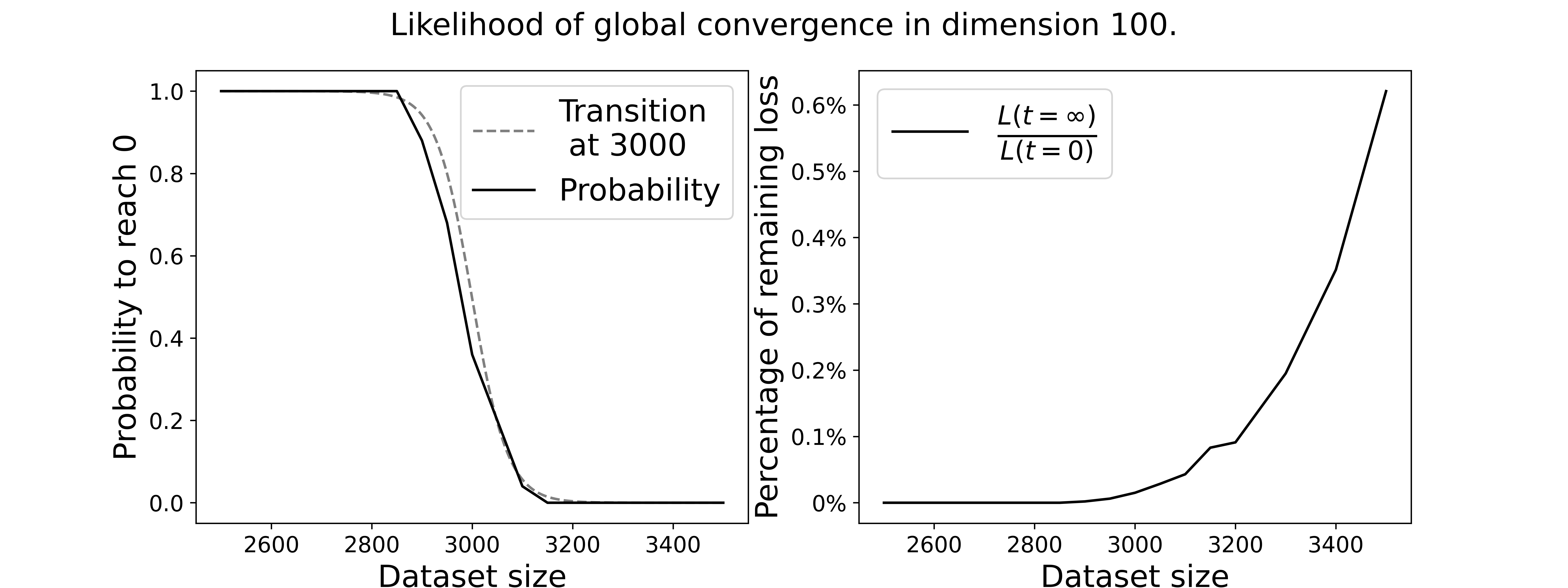
Figure 2: Left: Probability that a network trained on $n$ data converges to 0 loss. We observe a transition at $n=3000$, from likely to unlikely convergence.
Right: Loss at convergence normalized by the loss at initialization. For $n\geq 3000$, the loss increases to $0.6\%$, which is equivalent to fitting all but one example.

This section aims to test the limit in which Corollary 1 holds when the number of data points increase. Intuitively, as the number of examples $n$ grows, the neural network becomes less and less overparametrized, and hence is expected to fail to globally converge. Knowing if and when this occurs with high probability is important for us to understand how much our current threshold $C\sqrt{d}$ can be improved. We thus plot the probability of convergence, as well as the loss at convergence to obtain additional information when the probability is zero. We train $500$ one-layer neural networks with the normalization presented in Section 2, dimension $d=100$, $n$ ranging from $2500$ to $3500$, and $p_{n}=C\log(n)$ neurons. Additional details on the training procedure can be found in Appendix B.

Figure 2 shows that for $n\leq 2900$, the probability of convergence is very likely, for $n\geq 3100$ the probability is almost zero, and in between, there is a sharp transition. This sharp transition is visible for any value $d$ at some point $N(d,p)$, which we name the convergence threshold. By measuring the point for different values of $d$ and $p$, we see that the threshold scales like $N(d,p)\simeq C(p)d$, with $C(p)$ which is sub-linear (see Figure 4 in Appendix B). In particular, for $n\leq Cdp$, there exists a network that interpolates the data, meaning that the convergence threshold is not a threshold for the existence of a global minimum. The threshold’s scaling is linear in $d$ which implies that proving convergence for $Cd$ data in dimension $d$ seems feasible.

5.2 Empirical asymptotic local-PL curvature

In this section we test Conjecture 1, and to do so we measure $\mu(t)$ during the dynamics, and mostly at the end of the dynamics, since we know by Lemma 4 that near 0 the local-PL curvature is of order $\frac{1}{n}$. To provide the strongest evidence for the conjecture, we measured the order of the local-PL curvature in three ways: by directly measuring the local-PL $\mu(t_{\infty})=\log\left(\frac{L(t_{\infty}-1)}{L(t_{\infty})}\right)$ at the last epoch $t_{\infty}$, by measuring the average-PL curvature $\langle\mu_{\infty}\rangle=\frac{1}{t_{\infty}}\log\left(\frac{L(0)}{L(t_{\infty})}\right)$, and finally by mesuring the lower and upper bounds on the local-PL given in Lemma 6.

Following Conjecture 1, all approximations should likely be decreasing in $\frac{1}{\sqrt{n}}$ as $n$ increases. To show this, we plot the log-log graph of each measure above. We train $500$ networks in dimension $d=2000$, with $n$ ranging from $1000$ to $2000$, and $p_{n}=C\log(n)$. All resulting plots appear linear in the log-log scale, with a slope close to $-\frac{1}{2}$ (see Figure 5 in Appendix B), meaning that the scalings are indeed in $\frac{C}{\sqrt{n}}$. This empirically confirms our conjecture that the local-PL curvature has order $\frac{1}{\sqrt{n}}$ asymptotically.

6 Conclusion

We have studied the convergence of the gradient flow on a one-hidden-layer ReLU networks on finite datasets. Our analysis leverages a local Polyak-Łojasiewicz viewpoint on the gradient-flow dynamics, revealing that for a large dimension $d$ in the order of $n^{2}$ data points, we can guarantee global convergence with high probability using only $\log(n)$ neurons. The specificity of the system relies on the low-correlation between the input data due to the high dimension. Moreover, in the orthogonal setting the loss’s exponential rate of convergence is at least of order $\frac{1}{n}$ and at most of order $\frac{1}{\sqrt{n}}$, which is also the average asymptotic order as experimentally verified. For a special initialization of the network, a phase transition in this rate occurs during the dynamics.

Future Directions.

We are most enthusiastic about proving the convergence of the networks for linear threshold $d\geq Cn$, which should require new proof techniques, as well as quantifying the impact of large amounts of neurons on the system, which has been overlooked in our study. Future work should also consider a using a teacher-network to generate the outputs, in order to link the probability or interpolation with the complexity, in terms of neurons, of the teacher.

7 Acknowledgements

This work has received support from the French government, managed by the National Research Agency, under the France 2030 program with the reference "PR[AI]RIE-PSAI" (ANR-23-IACL-0008).

Organization of the Appendix

The appendices of this article are structured as follows. Appendix A contains the proofs of each of the 10 statements of the paper in an entitled subsection, with additional lemmas included in the relevant subsections. Only Corollary 1 doesn’t have a complete proof as it is a simple combination of Lemma 3 and Theorem 1. Appendix B contains additional details on the experiments that were performed in Section 5, as well as graphs for the scaling laws. Finally, Appendix C contains general discussions about the possibility to provably learn $2d$ inputs in dimension $d$, and the possible collapse of the second-layer weights.

Appendix A Proofs

A.1 Theorem 1

Lemma 5 shows that a number of neurons of order $\log(n)$ is both necessary and sufficient to obtain the event $\mathcal{I}$, which corresponds to a nice initialization of the network.

Lemma 5.

Suppose $y_{i}\neq 0$, and let $\mathcal{I}$ the event: for all $i$, there exists $j$ such that, $\langle w_{j}(0)|x_{i}\rangle>0$ and $a_{j}(0)y_{i}>0$. For all $\varepsilon>0$,

• if $p\geq 4\log(\frac{n}{\varepsilon})$, then $\mathbb{P}(\mathcal{I})\geq 1-\varepsilon$,

• if $p\leq 3\log(\frac{n}{\varepsilon})-2$, then $\mathbb{P}(\mathcal{I})\leq 1-\varepsilon$,

and thus, $\mathbb{P}(\mathcal{I})=1-\varepsilon$ implies $p\in[3\log(\frac{n}{\varepsilon})-2,4\log(\frac{n}{\varepsilon})]$.

Proof.

of Lemma 5
Let us note $\langle w_{j}(0)|x_{i}\rangle=W_{i,j}$ and $A_{j}=a_{j}(0)y_{i}$ random variables which are symmetric. $A_{j}$ are independent with all variables, while $W_{j,i}$ are independent with all variables $A_{j}$ and $W_{q,k}$ with $q\neq j$.

$$\begin{split}\mathbb{P}(\mathcal{I})&=\mathbb{P}(\forall i,\exists j,\langle w_{j}(0)|x_{i}\rangle>0\cap a_{j}y_{i}>0)\\ &=\mathbb{P}\left(\bigcap_{i}\bigcup_{j}W_{i,j}>0\cap A_{j}>0\right)\\ &=1-\mathbb{P}\left(\bigcup_{i}\bigcap_{j}W_{i,j}\leq 0\cup A_{j}\leq 0\right)\\ &\geq 1-n\mathbb{P}\left(\bigcap_{j}W_{i,j}\leq 0\cup A_{j}\leq 0\right)\\ &=1-n\mathbb{P}\left(W_{i,j}\leq 0\cup A_{j}\leq 0\right)^{p}\\ &=1-n(1-\mathbb{P}\left(W_{i,j}>0\cap A_{j}>0\right))^{p}\\ &=1-n\left(1-\mathbb{P}\left(W_{i,j}>0\right)\mathbb{P}\left(A_{j}>0\right)\right)^{p}\\ &=1-n\left(\frac{3}{4}\right)^{p}\\ \end{split}$$ (13)

Replacing the expression with $p=4\log(\frac{n}{\varepsilon})\geq\frac{1}{\frac{1}{3}-\frac{1}{2}\frac{1}{3^{2}}}\log(\frac{n}{\varepsilon})\geq\frac{\log(\frac{n}{\varepsilon})}{\log(\frac{4}{3})}$, we find that the probability is larger than $1-\varepsilon$. Now for the other bound,

$$\begin{split}\mathbb{P}(\mathcal{I})&=\mathbb{P}(\forall i,\exists j,\langle w_{j}(0)|x_{i}\rangle>0\cap a_{j}y_{i}>0)\\ &=\mathbb{P}\left(\bigcap_{i}\bigcup_{j}W_{i,j}>0\cap A_{j}>0\right)\\ &\leq\mathbb{P}\left(\bigcap_{i}\bigcup_{j}W_{i,j}>0\right)\\ &=\mathbb{P}\left(\bigcup_{j}W_{1,j}>0\right)^{n}\\ &=(1-\mathbb{P}\left(W_{1,1}>0\right)^{p})^{n}\\ &=(1-2^{-p})^{n}\\ &\leq\left(1-4\left(\frac{\varepsilon}{n}\right)^{3\log(2)}\right)^{n}\\ &\leq\left(1-4\frac{\varepsilon}{n}\right)^{n}\\ &\leq 1-\varepsilon\end{split}$$ (14)

where we use $(1-\frac{x}{n})^{n}\leq 1-\frac{x}{e}\leq 1-\frac{x}{4}$ valid on $x\in[0,1]$. ∎

Lemma 6.

For any set of parameters $\theta=(a_{j},w_{j})_{j=1:p}$, the following bounds on the local-PL curvature hold.

$$\begin{split}\mu(t)&\leq\frac{2}{n}(C_{x}^{+}+||X^{T}X-D_{X}||)\max_{i}\frac{1}{p}\sum_{j=1}^{p}(|a_{j}|^{2}+||w_{j}||^{2})1_{j,i}\\ \mu(t)&\geq\frac{2}{n}(C_{x}^{-}-||X^{T}X-D_{X}||)\min_{i}\frac{1}{p}\sum_{j=1}^{p}|a_{j}|^{2}1_{j,i}\end{split}$$ (15)

Proof.

of Lemma 6
Let us start by writing the derivatives of the two variables of the system. We define $P_{j}\in\mathbb{R}^{n\times n}$ the diagonal matrix with elements $1_{j,i}$.

$$\begin{split}&\frac{d}{dt}w_{j}=\frac{a_{j}}{n}\sum_{i=1}^{n}r_{i}x_{i}1_{j,i}=\frac{a_{j}}{n}XP_{j}R\\ &\frac{d}{dt}a_{j}=\frac{1}{n}\sum_{i=1}^{n}r_{i}\langle w_{j}|x_{i}\rangle_{+}=\frac{1}{n}w_{j}^{T}XP_{j}R\end{split}$$ (16)

We now compute the derivatives for the residuals $r_{i}$.

$$\begin{split}\frac{d}{dt}r_{i}&=-\frac{1}{p}\sum_{j=1}^{p}\left(\frac{d}{dt}a_{j}\right)\langle w_{j}|x_{i}\rangle_{+}+a_{j}\left(\frac{d}{dt}\langle w_{j}|x_{i}\rangle_{+}\right)\\ &=-\frac{1}{np}\sum_{j=1}^{p}1_{j,i}x_{i}^{T}w_{j}w_{j}^{T}XP_{j}R+|a_{j}|^{2}1_{j,i}x_{i}^{T}XP_{j}R\\ \frac{d}{dt}R&=-\frac{1}{np}\left[\sum_{j=1}^{p}P_{j}X^{T}w_{j}w_{j}^{T}XP_{j}+|a_{j}|^{2}P_{j}X^{T}XP_{j}\right]R\\ \end{split}$$ (17)

The matrix written between brackets is symmetric, and the local-PL curvature lies between its smallest and largest eigenvalues.

$$\frac{d}{dt}||R||^{2}=-\frac{2}{np}\left[\sum_{j=1}^{p}(w_{j}^{T}XP_{j}R)^{2}+|a_{j}|^{2}||XP_{j}R||^{2}\right]$$ (18)

Since $0\preceq w_{j}w_{j}^{T}\preceq||w_{j}||^{2}I_{d}$, we get the following bound on the derivative

$$-\frac{2}{np}\sum_{j=1}^{p}(||w_{j}||^{2}+|a_{j}|^{2})||XP_{j}R||^{2}\leq\frac{d}{dt}||R||^{2}\leq-\frac{2}{np}\sum_{j=1}^{p}|a_{j}|^{2}||XP_{j}R||^{2}$$ (19)

We can manipulate the term $||XP_{j}R||^{2}$ to make $||X^{T}X-D_{X}||$ appear.

$$\begin{split}||XP_{j}R||^{2}&=R^{T}P_{j}^{T}X^{T}XP_{j}R\\ &=R^{T}P_{j}^{T}(D_{X}-(X^{T}X-D_{X}))P_{j}R\\ &=||\sqrt{D_{X}}P_{j}R||^{2}-||\sqrt{X^{T}X-D_{X}}P_{j}R||^{2}\\ &\geq(C_{x}^{-})^{2}||P_{j}R||^{2}-||X^{T}X-D_{X}||||P_{j}R||^{2}\\ &\leq(C_{x}^{+})^{2}||P_{j}R||^{2}+||X^{T}X-D_{X}||||P_{j}R||^{2}\end{split}$$ (20)

Finally, by observing that $\mu(t)=\frac{\frac{d}{dt}||R||^{2}}{||R|^{2}}$, one has the lower bound

$$\begin{split}\mu(t)&\geq\frac{2}{np}\sum_{j=1}^{p}|a_{j}|^{2}\frac{||P_{j}R||^{2}}{||R||^{2}}\left((C_{x}^{-})^{2}-||X^{T}X-D_{X}||\right)\\ &\geq\frac{2}{n}\frac{1}{||R||^{2}}\left((C_{x}^{-})^{2}-||X^{T}X-D_{X}||\right)\sum_{i=1}^{n}\frac{r_{i}^{2}}{p}\sum_{j=1}^{p}|a_{j}|^{2}1_{j,i}\\ &\geq\frac{2}{n}\left((C_{x}^{-})^{2}-||X^{T}X-D_{X}||\right)\min_{i}\frac{1}{p}\sum_{j=1}^{p}|a_{j}|^{2}1_{j,i},\\ \end{split}$$ (21)

and and the upper bound

$$\begin{split}\mu(t)&\leq\frac{2}{np}\sum_{j=1}^{p}|a_{j}|^{2}\frac{||P_{j}R||^{2}}{||R||^{2}}\left((C_{x}^{+})^{2}+||X^{T}X-D_{X}||\right)\\ &\leq\frac{2}{n}\left((C_{x}^{+})^{2}+||X^{T}X-D_{X}||\right)\max_{i}\frac{1}{p}\sum_{j=1}^{p}(|a_{j}|^{2}+||w_{j}||^{2})1_{j,i}.\\ \end{split}$$ (22)

∎

Proof.

of Theorem 1
This is a precise proof based on the sketch visible in Section 3. The proof of convergence relies on three key points:

1. The loss strictly decreases as long as each example is activated by at least a neuron.

2. For a data point, if there exists a neuron which is activated at initialization, then at least one neuron remains activated throughout the dynamics.

3. At initialization, the previous condition is satisfied with large probability.

We finish the proof with the lower bounds on $\mu(t)$ and $\langle\mu_{\infty}\rangle$.

(i) First, Lemma 6 shows that, by computing the derivatives of the loss, we get a lower bound on the curvature.

$$\mu(t)\geq\frac{2}{n}\left((C_{x}^{-})^{2}-||X^{T}X-D_{X}||\right)\min_{i}\left\{\frac{1}{p}\sum_{j=1}^{p}|a_{j}|^{2}1_{j,i}\right\}$$ (23)

We want to show the strict positivity of this lower bound. First, using Assumption 2, we have for all $n\geq 2$ that

$$(C_{x}^{-})^{2}-||X^{T}X-D_{X}||\geq(C_{x}^{-})^{2}\left(1-\frac{1}{\sqrt{n}}\frac{C_{y}^{-}}{C_{y}^{+}}\right)\geq\left(1-\frac{1}{\sqrt{2}}\right)(C_{x}^{-})^{2}$$ (24)

which also holds for $n=1$ since then $||X^{T}X-D_{X}||=0$. Moreover, thanks to the asymmetric initialization, we have $|a_{j}|^{2}\geq|a_{j}(0)|^{2}-||w_{j}(0)||^{2}>0$, which means that $\mu(t)$ is bounded away from 0 as long as for all $i$ there exists $j$ satisfying $\langle w_{j}(t)|x_{i}\rangle_{+}>0$.

(ii) Let us fix the data index $i\in\llbracket 1,n\rrbracket$, and $y_{i}>0$ without loss of generality. Let us define $j^{*}_{i}\leavevmode\nobreak\ =\leavevmode\nobreak\ \arg\max_{a_{j}y_{i}>0}\langle w_{j}(t)|x_{i}\rangle$ the index of the largest correctly initialized neuron. Since $a_{j}$ cannot change sign thanks to Assumption 1, $\langle w_{j_{i}^{*}}(t)|x_{i}\rangle$ is continuous, and has a derivative over each constant segment of $j_{i}^{*}$. We can write the derivatives of this neuron as

$$\begin{split}\frac{d}{dt}\langle w_{j_{i}^{*}}|x_{i}\rangle&=\frac{a_{j_{i}^{*}}}{n}\sum_{k}^{n}r_{k}\langle x_{i}|x_{k}\rangle 1_{{j_{i}^{*}},k}\\ &=\frac{a_{j_{i}^{*}}}{n}e_{i}^{T}X^{T}XP_{j}R\\ &\geq\frac{|a_{j_{i}^{*}}|}{n}\left[r_{i}||x_{i}||^{2}1_{{j_{i}^{*}},i}s_{j_{i}^{*}}-||X^{T}X-D_{X}||||R||\right]\\ &=\frac{|a_{j_{i}^{*}}|}{n}\left[r_{i}||x_{i}||^{2}1_{{j_{i}^{*}},i}s_{j_{i}^{*}}-||X^{T}X-D_{X}||\sqrt{2nL(\theta_{t})}\right]\\ &\geq\frac{|a_{j_{i}^{*}}|}{n}\left[r_{i}||x_{i}||^{2}1_{{j_{i}^{*}},i}s_{j_{i}^{*}}-||X^{T}X-D_{X}||\sqrt{2nL(\theta(0))}\right]\\ \end{split}$$ (25)

With the condition $||X^{T}X-D_{X}||<\frac{1}{\sqrt{n}}(C_{x}^{-})^{2}\frac{C_{y}^{-}}{C_{y}^{+}}$ and the fact that $s_{j_{i}^{*}}y_{i}>0$, we get the inequality

$$\begin{split}\frac{d}{dt}\langle w_{s_{j_{i}^{*}}}|x_{i}\rangle&>\frac{|a_{s_{j_{i}^{*}}}|C_{y}^{-}(C_{x}^{-})^{2}}{n}\left[\frac{r_{i}}{y_{i}}1_{s_{j_{i}^{*}},i}-1\right]\\ \end{split}$$ (26)

Now, the strict positivity of $\langle w_{j_{i}^{*}}|x_{i}\rangle$ is an invariant of the system: if $\frac{r_{i}}{y_{i}}\geq 1$, then $\langle w_{j_{i}^{*}}|x_{i}\rangle$ strictly increases, and otherwise we have

$$0<\frac{y_{i}-r_{i}}{y_{i}}=\frac{1}{p}\sum_{j=1}^{p}\frac{a_{j}}{y_{i}}\langle w_{j}|x_{i}\rangle_{+}\leq\langle w_{j_{i}^{*}(t)}|x_{i}\rangle\frac{1}{p}\sum_{j=1}^{p}\frac{|a_{j}|}{|y_{i}|}$$ (27)

Which implies that $\langle w_{j_{i}^{*}}|x_{i}\rangle$ stays strictly positive throughout the dynamics.

(iii) As shown in Lemma 5, for $p\geq 4\log(\frac{n}{\varepsilon})$, we have the strict positivity with probability $1-\varepsilon$.

$$\mathbb{P}(\forall i,\exists j,\langle w_{j}(0)|x_{i}\rangle>0\cap a_{j}y_{i}>0)\geq 1-\varepsilon.$$ (28)

Finally, we prove the lower bounds on the PL. Let us recall that $|a_{j}|\geq||w_{j}||$ and that $1_{j,i}\geq\langle\bar{w}_{j}(t)|\bar{x}_{i}\rangle_{+}$, which gives us

$$\frac{1}{p}\sum_{j=1}^{p}|a_{j}|^{2}1_{j,i}\geq\left|\frac{1}{p}\sum_{j=1}^{p}a_{j}\langle w_{j}|\bar{x}_{i}\rangle_{+}\right|=\left|\frac{y_{i}-r_{i}(t)}{C_{x}^{+}}\right|.$$ (29)

We can plug these into equation 23 to obtain

$$\mu(t)\geq\frac{2-\sqrt{2}}{n}\frac{(C_{x}^{-})^{2}}{C_{x}^{+}}C_{y}^{-}\min_{i}\left|1-\frac{r_{i}(t)}{y_{i}}\right|$$ (30)

From this last equation, by integration, we obtain

$$\frac{1}{t}\int_{0}^{t}\mu(u)du\geq\frac{2-\sqrt{2}}{n}\frac{(C_{x}^{-})^{2}}{C_{x}^{+}}C_{y}^{-}\left(1-\frac{1}{t}\int_{0}^{t}\max_{i}\left|\frac{r_{i}(u)}{y_{i}}\right|du\right)$$ (31)

Let $t_{\delta}$ satisfying $\max_{i}|r_{i}(t)|\leq\delta$ for all $t\geq t_{\delta}$. $t_{\delta}$ exists and is finite since the loss reaches 0. Thus, we have for any $\delta>0$ that

$$\frac{1}{t}\int_{0}^{t}\mu(u)du\geq\frac{2-\sqrt{2}}{n}\frac{(C_{x}^{-})^{2}}{C_{x}^{+}}C_{y}^{-}\left(1-\frac{t_{\delta}}{t}\max_{i}\frac{\sqrt{2nL(\theta_{0})}}{\left|y_{i}\right|\sqrt{p}}-\frac{t-t_{\delta}}{t}\delta\right)$$ (32)

whic in the limit $t\rightarrow+\infty$ gives

$$\langle\mu_{\infty}\rangle\geq\frac{2-\sqrt{2}}{n}\frac{(C_{x}^{-})^{2}}{C_{x}^{+}}C_{y}^{-}(1-\delta)$$ (33)

Taking $\delta\rightarrow 0$ gives the desired bound. ∎

A.2 Lemma 3

Proof.

of Lemma 3
This proof will heavily rely on the result of Vershynin [2010, Remark 5.59] on the concentration of sub-Gaussian random variables. It states that if $A\in\mathbb{R}^{n\times d}$ is a matrix, the columns of which are $n$ independent centered, whitened, sub-Gaussian random variables in dimension $d$, then with probability $1-2e^{-t^{2}}$,

$$\left|\left|\frac{1}{d}A^{T}A-I_{d}\right|\right|\leq C\sqrt{\frac{n}{d}}+\frac{t}{\sqrt{d}}$$ (34)

with $C>0$ depending only on $\max_{i}||A_{i}||_{\psi_{2}}$ the sub-Gaussian norm of the columns. We use this property with $A_{i}=\frac{\sqrt{d}}{\lambda}x_{i}$ which satisfies every hypothesis, in particular it is whitened since by assumption $\mathbb{E}[x_{i}x_{i}^{T}]=\frac{\lambda^{2}}{d}I_{d}$, and $t=\sqrt{\log\left(\frac{2}{\varepsilon}\right)}$, which gives

$$\left|\left|\frac{1}{\lambda^{2}}X^{T}X-I_{d}\right|\right|=\left|\left|\frac{1}{d}A^{T}A-I_{d}\right|\right|\leq C\sqrt{\frac{n}{d}}+\sqrt{\frac{\log\left(\frac{2}{\varepsilon}\right)}{d}}$$ (35)

Moreover, note that

$$(C_{x}^{-})^{2}\geq 1+\min_{i}(||x_{i}||^{2}-1)\geq 1-||X^{T}X-I_{d}||$$ (36)

Thus, the condition in Assumption 2 is satisfied if

$$\left|\left|X^{T}X-\lambda^{2}I_{d}\right|\right|\leq\lambda\frac{C_{y}^{-}}{C_{y}^{-}+\sqrt{n}C_{y}^{+}}$$ (37)

Now, since $C_{y}^{-},C_{y}^{+}$ are independent of $n$ since $\mathcal{P}_{Y}$ has compact support away from 0, taking

$$d>16n\max\left(C^{2}n,\log\left(\frac{2}{\varepsilon}\right)\right)\left(\frac{C_{y}^{-}}{C_{y}^{+}}\right)^{2}$$ (38)

is sufficient for Assumption 2 with probability $1-\varepsilon$. ∎

The proof of Corollary 1 is then the combination of the proof of Theorem 1, using $\left|\left|X^{T}X-\lambda^{2}I_{d}\right|\right|$ instead of $||XX^{T}-D_{X}||$, with $\frac{\varepsilon}{2}$.

A.3 Proposition 1

Lemma 7.

Suppose orthogonal inputs and convergence of the system to 0 loss, then with probability $1-\varepsilon$ for all $t\geq t_{n}$ with $t_{n}=2n\max_{j,i}\frac{\langle w_{j}(0)|x_{i}\rangle_{+}}{|y_{i}|||x_{i}||^{2}(|a(0)|^{2}-||w_{j}(0)||^{2})}$,

$$\begin{split}a_{j}(0)y_{i}>0&\implies\langle w_{j}(t)|x_{i}\rangle_{+}\geq\langle w_{j}(0)|x_{i}\rangle_{+}\\ a_{j}(0)y_{i}<0&\implies\langle w_{j}(t)|x_{i}\rangle_{+}\leq 0\\ \end{split}$$ (39)

This Lemma states that, for orthogonal data, incorrectly initialized neuron vanish, and cannot become active again. Thus, after time $t_{n}$, the system is decoupled between the positive and negative labels, and only correctly initialized neuron, which are useful to the prediction, persist.

Proof.

of Lemma 7
We start by computing the derivative of a neuron in the orthogonal setting.

$$\begin{split}\frac{d}{dt}\langle w_{j}|x_{i}\rangle_{+}&=\frac{a_{j}r_{i}1_{j,i}||x_{i}||^{2}}{n}\\ \frac{d}{dt}a_{j}&=\frac{1}{n}\sum_{i=1}^{n}r_{i}\langle w_{j}|x_{i}\rangle_{+}\end{split}$$ (40)

Let us only discuss the case of neurons that are positive at initialization since otherwise nothing happens. We observe that, as long as all $r_{i}\neq 0$, then the neurons vary monotonously. This implies that if $a_{j}y_{i}<0$, then the corresponding neuron will reach 0 in finite time. Let $t^{*}_{n}$ the first time any $|r_{i}-y_{i}|=\frac{y_{i}}{2}$, which is finite with high probability. For $j,i$ such that $a_{j}y_{i}<0$, we have

$$\begin{split}\frac{d}{dt}\langle w_{j}|x_{i}\rangle_{+}&\leq-\frac{\sqrt{|a_{j}(0)|^{2}-||w_{j}(0)||^{2}}|y_{i}|}{2n}||x_{i}||^{2}1_{j,i}\\ \langle w_{j}|x_{i}\rangle_{+}&\leq\langle w_{j}(0)|x_{i}\rangle_{+}-1_{j,i}\frac{|y_{i}|}{2n}||x_{i}||^{2}C_{j}t\end{split}$$ (41)

where $C_{j}^{2}=|a_{j}(0)|^{2}-||w_{j}(0)||^{2}$. Let $\tilde{t}_{n}=\max_{j,i}\frac{2n\langle w_{j}(0)|x_{i}\rangle_{+}}{|y_{i}||x_{i}||^{2}C_{j}}$, if $\tilde{t}_{n}\leq t^{*}_{n}$, then we have extinction in finite time, i.e., the incorrectly initialized neurons have reached 0. Let us show that at $\tilde{t}_{n}$, residuals have almost not moved. First, we bound the second-layer neurons $a_{j}$,

$$\begin{split}\frac{d}{dt}a_{j}&\leq\frac{1}{n}\sqrt{\sum_{i=1}^{n}r_{i}^{2}}\sqrt{\sum_{i=1}^{n}\langle w_{j}|x_{i}\rangle_{+}^{2}}\\ &\leq\sqrt{2}L(\theta_{t})\max_{i}\langle w_{j}|x_{i}\rangle_{+}\\ &\leq\sqrt{2}L(\theta_{0})\max_{i}\langle w_{j}|x_{i}\rangle_{+}\\ a_{j}-a_{j}(0)&\leq\sqrt{2}L(\theta_{0})\int_{0}^{t}\max_{i}\langle w_{j}(u)|x_{i}\rangle_{+}du\end{split}$$ (42)

Let $C_{1}=\frac{3}{2n}\max_{i}|y_{i}|||x_{i}||^{2}$, $C_{2}=\max_{i}\langle w_{j}(0)|x_{i}\rangle_{+}^{2}+a_{j}(0)^{2}\frac{C_{1}}{2}$, and $C_{3}=C_{1}\left(\frac{L(\theta_{0})}{\sqrt{2}}+\frac{1}{2}\right)$. The upper bound on $a_{j}$ turns into an upper bound on $w_{j}$,

$$\begin{split}\frac{d}{dt}\max_{i}\langle w_{j}(u)|x_{i}\rangle_{+}&\leq C_{1}\left(a_{j}(0)+\sqrt{2}L(\theta_{0})\int_{0}^{t}\max_{i}\langle w_{j}(u)|x_{i}\rangle_{+}du\right)\\ \max_{i}\langle w_{j}(t)|x_{i}\rangle_{+}^{2}-\max_{i}\langle w_{j}(0)|x_{i}\rangle_{+}^{2}&\leq C_{1}a_{j}(0)\int_{0}^{t}\max_{i}\langle w_{j}(u)|x_{i}\rangle_{+}du+\\ &+\frac{C_{1}}{\sqrt{2}}L(\theta_{0})\int_{0}^{t}\max_{i}\langle w_{j}(u)|x_{i}\rangle_{+}^{2}du\\ \max_{i}\langle w_{j}(t)|x_{i}\rangle_{+}^{2}&\leq C_{2}+C_{3}\int_{0}^{t}\max_{i}\langle w_{j}(u)|x_{i}\rangle_{+}^{2}du\\ \end{split}$$ (43)

Let us pose $A_{j}(t)=\int_{0}^{t}\max_{i}\langle w_{j}(u)|x_{i}\rangle_{+}^{2}du$, We can solve the differential inequality

$$\begin{split}A_{j}^{\prime}(t)&\leq C_{2}+C_{3}A_{j}(t)\\ A_{j}(t)+\frac{C_{2}}{C_{3}}&\leq(A_{j}(0)+\frac{C_{2}}{C_{3}})e^{C_{3}t}\end{split}$$ (44)

In the end, we obtain

$$\max_{i}\langle w_{j}|x_{i}\rangle_{+}\leq C_{2}e^{C_{3}t}$$ (45)

Importantly, since $C_{3}\tilde{t}_{n}$ is a constant of $n$, we have that at there exists $K_{1},K_{2}$ which doesn’t depend on $n$ such that at $\tilde{t}_{n}$ for all $j,i$,

$$\begin{split}\langle w_{j}(\tilde{t}_{n})|x_{i}\rangle_{+}&\leq K_{1}\langle w_{j}(0)|x_{i}\rangle_{+}\\ |a_{j}|&\leq K_{2}|a_{j}(0)|\\ \end{split}$$ (46)

Thus, we can bound the deviation of the residuals at the beginning of the dynamics.

$$\begin{split}|r_{i}(\tilde{t}_{n})-y_{i}|&=\left|\frac{1}{p}\sum_{j=1}^{p}a_{j}\langle w_{j}|x_{i}\rangle_{+}\right|\\ &\leq\frac{1}{p}\sum_{j=1}^{p}\left|a_{j}\right|\langle w_{j}|x_{i}\rangle_{+}\\ &\leq K_{1}K_{2}\frac{1}{p}\sum_{j=1}^{p}\left|a_{j}(0)\right|\langle w_{j}(0)|x_{i}\rangle_{+}\end{split}$$ (47)

Finally, since $a_{j},w_{j}$ are initialized with norms independent of $d$, it means that by rotational invariance $\langle w_{j}(0)|x_{i}\rangle$ has variance $\frac{1}{\sqrt{d}}$ and mean 0. Thus, in large dimension, we get that $|r_{i}(\tilde{t}_{n})-y_{i}|\underset{d\rightarrow+\infty}{\rightarrow}0$. This shows that for $d$ sufficiently large, we have $\tilde{t}_{n}\leq t^{*}_{n}$. ∎

Proof.

of Proposition 1
Thanks to Lemma 7, there exists $t_{n}$ such that for $t\geq t_{n}$, each example has only correctly activated neurons. Without loss of generality suppose that all labels are positive. Then the network only has positive contributions $a_{j}(t)\langle w_{j}|x_{i}\rangle\geq 0$ for all i. Let $N(j,i)$ the number of indices $q$ such that $a_{j}(t)\langle w_{j}|x_{i}\rangle\leq a_{q}(t)\langle w_{q}|x_{i}\rangle$. We have

$$\frac{N(j,i)}{p}a_{j}\langle w_{j}|x_{i}\rangle\leq\frac{1}{p}\sum_{q=1}^{p}a_{q}\langle w_{q}|x_{i}\rangle=y_{i}-r_{i}$$ (48)

Thus, we can bound the norm of $w_{j}$,

$$\begin{split}||w_{j}||^{4}&\leq a_{j}^{2}||w_{j}||^{2}\\ &=\sum_{i=1}^{n}a_{j}^{2}\langle w_{j}|\bar{x}_{i}\rangle^{2}\\ &\leq\sum_{i=1}^{n}\frac{p^{2}}{N(j,i)^{2}}\left(\frac{y_{i}-r_{i}}{||x_{i}||}\right)^{2}\\ &\leq\max_{i}\left(\frac{y_{i}-r_{i}}{C_{x}^{-}}\right)^{2}\sum_{i=1}^{n}\frac{p^{2}}{N(j,i)^{2}}\end{split}$$ (49)

This helps us majorate the sum of $|a_{j}|^{2}+||w_{j}||^{2}$

$$\begin{split}\frac{1}{p}\sum_{j=1}^{p}\left(|a_{j}|^{2}+||w_{j}||^{2}\right)1_{j,i}&\leq\frac{1}{p}\sum_{j=1}^{p}\left(|a_{j}(0)|^{2}-||w_{j}(0)||^{2}\right)1_{j,i}+\frac{2}{p}\sum_{j=1}^{p}||w_{j}||^{2}\\ &\leq\bar{C}+\frac{2}{p}\sum_{j=1}^{p}\frac{\max_{i}(y_{i}-r_{i})}{C_{x}^{-}}\sqrt{\sum_{i=1}^{n}\frac{p^{2}}{N(j,i)^{2}}}\\ &\leq\bar{C}+2\frac{\max_{i}(y_{i}-r_{i})}{C_{x}^{-}}\sum_{j=1}^{p}\sqrt{\sum_{i=1}^{n}\frac{1}{N(j,i)^{2}}}\\ &\leq\bar{C}+\pi\sqrt{\frac{2}{3}}\frac{\max_{i}(y_{i}-r_{i})}{C_{x}^{+}}\sqrt{np}\\ &\leq\bar{C}+6\frac{\max_{i}(y_{i}-r_{i})}{C_{x}^{-}}\sqrt{np}\\ \end{split}$$ (50)

which we can use in the bound from Lemma 6 to end the proof. Thus, the constant $C$ from the Proposition statement is

$$\begin{split}C=\max\bigg{(}&2\max_{j,i}\frac{\langle w_{j}(0)|x_{i}\rangle_{+}}{|y_{i}|||x_{i}||^{2}(|a(0)|^{2}-||w_{j}(0)||^{2})},\\ &2(C_{x}^{+})^{2}\frac{1}{p}\sum_{j=1}^{p}\left(|a_{j}(0)|^{2}-||w_{j}(0)||^{2}\right)1_{j,i},\\ &12\frac{(C_{x}^{+})^{2}}{C_{x}^{-}}C_{y}^{+}\bigg{)}\end{split}$$ (51)

∎

A.4 Proposition 2

Proof.

of Proposition 2
Recall that the number of neurons is the number of groups $p_{n}k_{n}=n$, that we have for $q\neq j$ that $\langle w_{j}|x_{i}^{q}\rangle\leq 0$ at all time, meaning that $h_{\theta}(x_{i}^{j})=\frac{a_{j}}{p_{n}}\langle w_{j}|x_{i}^{j}\rangle_{+}=\frac{s_{j}}{p_{n}}||w_{j}||_{+}\langle w_{j}|x_{i}^{j}\rangle_{+}$, and $s_{j}$ does not change by Lemma 1. This implies that the dynamics is decoupled: $w_{j}$ and $w_{q}$ can be studied separately.

Let us compute the dynamics for the neuron $j$. We let $D_{j}^{n}=\frac{1}{k_{n}}\sum_{i=1}^{k_{n}}y_{i}^{j}x_{i}^{j}$, $||w_{j}||_{+}^{2}=\sum_{i=1}^{n}\langle w_{j}|x_{i}\rangle_{+}^{2}$, and $\bar{x}^{+}=\frac{x}{||x||_{+}}$. We first consider the alignment between $w_{j}$ and $D_{j}^{n}$:

$$\begin{split}\frac{d}{dt}\langle\bar{D}_{j}^{n}|s_{j}\bar{w}^{+}_{j}\rangle&=\left\langle\bar{D}_{j}^{n}\big{|}I_{d}-\bar{w}^{+}_{j}(\bar{w}^{+}_{j})^{T}\big{|}\frac{1}{||w_{j}||_{+}}\frac{d}{dt}w_{j}\right\rangle\\ &=\frac{1}{n}\langle\bar{D}_{j}^{n}|I_{d}-\bar{w}^{+}_{j}(\bar{w}^{+}_{j})^{T}|R\rangle\\ &=\frac{1}{n}\langle\bar{D}_{j}^{n}|I_{d}-\bar{w}^{+}_{j}(\bar{w}^{+}_{j})^{T}|k_{n}D_{j}^{n}-\frac{s_{j}}{p_{n}}||w_{j}||_{+}w_{j}\rangle\\ &=\frac{\sqrt{k_{n}}||D_{j}^{n}||}{n}(1-\langle\bar{D}_{j}^{n}|s_{j}\bar{w}^{+}_{j}\rangle^{2})\\ \end{split}$$ (52)

This equation can be solved closed-form, and we obtain

$$\begin{split}\langle\bar{D}_{j}^{n}|s_{j}\bar{w}^{+}_{j}\rangle&=\frac{\sinh\left(c_{n}^{j}t\right)+\langle\bar{D}_{j}^{n}|s_{j}\bar{w}^{+}_{j}(0)\rangle\cosh\left(c_{n}^{j}t\right)}{\cosh\left(c_{n}^{j}t\right)+\langle\bar{D}_{j}^{n}|s_{j}\bar{w}^{+}_{j}(0)\rangle\sinh\left(c_{n}^{j}t\right)}\\ &=\frac{1}{c_{n}^{j}}\frac{d}{dt}\left[\log\left(\cosh\left(c_{n}^{j}t\right)+\langle\bar{D}_{j}^{n}|s_{j}\bar{w}^{+}_{j}(0)\rangle\sinh\left(c_{n}^{j}t\right)\right)\right]\end{split}$$ (53)

with $c_{n}^{j}=\frac{2\sqrt{k_{n}}||D_{j}^{n}||}{n}$. Now we can compute the norm of the neuron.

$$\begin{split}\frac{d}{dt}||w_{j}||_{+}^{2}&=2||w_{j}||_{+}\frac{s_{j}}{n}\sum_{i=1}^{k}r_{i}\langle w_{j}|x_{i}\rangle_{+}\\ &=\frac{2}{n}||w_{j}||_{+}^{2}(\langle D_{j}^{n}|s_{j}\bar{w}^{+}_{j}\rangle-\frac{1}{p_{n}}||w_{j}||_{+}^{2})\\ ||w_{j}||_{+}^{2}e^{\frac{2}{np_{n}}\int_{0}^{t}||w_{j}(u)||_{+}^{2}du}&=||w_{j}(0)||_{+}^{2}e^{\frac{2}{n}\int_{0}^{t}\langle D_{j}^{n}|s_{j}\bar{w}^{+}_{j}(u)\rangle du}\\ e^{\frac{2}{np_{n}}\int_{0}^{t}||w_{j}(u)||_{+}^{2}du}-1&=\frac{2}{np_{n}}||w_{j}(0)||_{+}^{2}\int_{0}^{t}e^{\frac{2}{n}\int_{0}^{u}\langle D_{j}^{n}|s_{j}\bar{w}^{+}_{j}(v)\rangle dv}du\\ ||w_{j}(t)||_{+}^{2}&=\frac{||w_{j}(0)||_{+}^{2}e^{\frac{2}{n}\int_{0}^{t}\langle D_{j}^{n}|s_{j}\bar{w}^{+}_{j}(u)\rangle du}}{1+\frac{2}{np_{n}}||w_{j}(0)||_{+}^{2}\int_{0}^{t}e^{\frac{2}{n}\int_{0}^{u}\langle D_{j}^{n}|s_{j}\bar{w}^{+}_{j}(v)\rangle dv}du}\end{split}$$ (54)

Finally, we can replace the expression of the correlation.

$$||w_{j}(t)||_{+}^{2}=\frac{p_{n}\sqrt{k_{n}}||D_{j}^{n}||||w_{j}(0)||_{+}^{2}\left(\cosh\left(c_{n}^{j}t\right)+\langle\bar{D}_{j}^{n}|s_{j}\bar{w}^{+}_{j}(0)\rangle\sinh\left(c_{n}^{j}t\right)\right)}{p_{n}\sqrt{k_{n}}||D_{j}^{n}||+||w_{j}(0)||_{+}^{2}\left(\sinh\left(c_{n}^{j}t\right)+\langle\bar{D}_{j}^{n}|s_{j}\bar{w}^{+}_{j}(0)\rangle(\cosh\left(c_{n}^{j}t\right)-1)\right)}$$ (55)

We use this equation in Lemma 6, and easily obtain the upper bound thanks to the monotonicity of $||w_{j}(t)||^{2}$.

$$\mu(t)\leq\frac{4}{np_{n}}\max_{i}\sum_{j}^{p}||w_{j}(t)||_{+}^{2}1_{j,i}=\frac{4\max_{j}||w_{j}(t)||_{+}^{2}}{np_{n}}\leq\frac{4C_{y}^{+}\sqrt{k_{n}}}{n}=\frac{4C_{y}^{+}}{n^{\alpha}}$$ (56)

For the lower bound, we have the bound for $t\geq\frac{\alpha}{2C_{y}^{-}}n^{3\alpha-1}\log\left(n(C_{y}^{+})^{\frac{1}{\alpha}}\right)\geq\frac{1}{c_{n}^{j}}\log(p_{n}\sqrt{k_{n}}||D_{j}^{n}||)$ by monotonicity. Indeed,

$$\cosh\left(c_{n}^{j}t\right)+\langle\bar{D}_{j}^{n}|s_{j}\bar{w}^{+}_{j}(0)\rangle\sinh\left(c_{n}^{j}t\right)\geq\frac{1}{2}e^{c_{n}^{j}t}\left(1+\langle\bar{D}_{j}^{n}|s_{j}\bar{w}^{+}_{j}(0)\rangle\right)$$ (57)

and

$$\sinh\left(c_{n}^{j}t\right)+\langle\bar{D}_{j}^{n}|s_{j}\bar{w}^{+}_{j}(0)\rangle(\cosh\left(c_{n}^{j}t\right)-1)\leq\frac{1}{2}e^{c_{n}^{j}t}\left(1+\langle\bar{D}_{j}^{n}|s_{j}\bar{w}^{+}_{j}(0)\rangle\right)$$ (58)

which implies that

$$\begin{split}||w_{j}(t)||_{+}^{2}&\geq\frac{p_{n}\sqrt{k_{n}}||D_{j}^{n}||||w_{j}(0)||_{+}^{2}e^{c_{n}^{j}t}\left(1+\langle\bar{D}_{j}^{n}|s_{j}\bar{w}^{+}_{j}(0)\rangle\right)}{2p_{n}\sqrt{k_{n}}||D_{j}^{n}||+||w_{j}(0)||_{+}^{2}e^{c_{n}^{j}t}\left(1+\langle\bar{D}_{j}^{n}|s_{j}\bar{w}^{+}_{j}(0)\rangle\right)}\\ &\geq p_{n}\sqrt{k_{n}}||D_{j}^{n}||\frac{||w_{j}(0)||_{+}^{2}\left(1+\langle\bar{D}_{j}^{n}|s_{j}\bar{w}^{+}_{j}(0)\rangle\right)}{2+||w_{j}(0)||_{+}^{2}\left(1+\langle\bar{D}_{j}^{n}|s_{j}\bar{w}^{+}_{j}(0)\rangle\right)}\\ &\geq p_{n}\sqrt{k_{n}}||D_{j}^{n}||\frac{||w_{j}(0)||_{+}^{2}}{2+||w_{j}(0)||_{+}^{2}}\end{split}$$ (59)

since $\langle\bar{D}_{j}^{n}|s_{j}\bar{w}^{+}_{j}(0)\rangle\geq 0$. Finally, we obtain the desired lower bound.

$$\mu(t)\geq\frac{2}{np_{n}}\min_{i}\sum_{j}^{p}||w_{j}(t)||_{+}^{2}1_{j,i}=\frac{2\min_{j}||w_{j}(t)||_{+}^{2}}{np_{n}}\geq\frac{2C_{y}^{-}}{n^{\alpha}}\min_{j}\frac{||w_{j}(0)||_{+}^{2}}{2+||w_{j}(0)||_{+}^{2}}$$ (60)

∎

A.5 Lemma 4

Proof.

of Lemma 4
Let us recall the equation of the local-PL curvature on the system.

$$\mu(0)=\frac{2}{np}\sum_{j=1}^{p}(w_{j}(0)XP_{j}R(0))^{2}+|a_{j}(0)|^{2}||XP_{j}R(0)||^{2}$$ (61)

Here there are 3 types of variables: $w_{j}$, $a_{j}$ and $P_{j}$ which is the diagonal matrix with diagonal $1_{j,i}$. We apply the Central Limit Theorem on the average on $p$ to find the limit law of $\mu(0)$. Let us first look at the residual limit at $t=0$ for large $p$.

$$R(0)=Y-\frac{1}{p}\sum_{j=1}^{p}a_{j}w_{j}^{T}XP_{j}=Y-\mathbb{E}[aw^{T}XP]-\frac{\xi_{p}}{\sqrt{p}}=\tilde{Y}-\frac{\xi_{p}}{\sqrt{p}}$$ (62)

With $\xi_{p}\underset{p\rightarrow+\infty}{\longrightarrow}\xi\sim\mathcal{N}(0,\mathbb{V}(aw^{T}XP))$. We split the residuals in the expression of $\mu(0)$.

$$\begin{split}(w_{j}^{T}XP_{j}R)^{2}&=(w_{j}^{T}XP_{j}\tilde{Y})^{2}-\frac{2}{\sqrt{p}}\tilde{Y}^{T}(w_{j}^{T}XP_{j})^{T}(w_{j}^{T}XP_{j})\xi_{p}+\frac{1}{p^{2}}(w_{j}^{T}XP_{j}\xi_{p})^{2}\\ ||XP_{j}R||^{2}&=||XP_{j}\tilde{Y}||^{2}-\frac{2}{\sqrt{p}}\tilde{Y}^{T}(XP_{j})^{T}(XP_{j})\xi_{p}+\frac{1}{p^{2}}||XP_{j}\xi_{p}||^{2}\\ \end{split}$$ (63)

This means that we can compute the average

$$\mu(0)\underset{p\rightarrow+\infty}{\longrightarrow}\frac{2}{n}\mathbb{E}[(w^{T}XP\tilde{Y})^{2}+|a|^{2}||XP\tilde{Y}||^{2}]=\frac{2}{n}\beta_{0}$$ (64)

and the deviation, as the deviation of the central terms and the first order deviations of the residuals,

$$\sqrt{p}(\mu(0)-\frac{2}{n}\beta_{0})\underset{p\rightarrow+\infty}{\longrightarrow}\mathcal{N}(0,\gamma_{0}^{2})$$ (65)

with

$$\begin{split}\gamma_{0}^{2}&=\mathbb{V}((w^{T}XP\tilde{Y})^{2}+|a|^{2}||XP\tilde{Y}||^{2})\\ &+\left|\left|\sqrt{\mathbb{V}(\xi)}\mathbb{E}[(w^{T}XP)^{T}(w^{T}XP)]\tilde{Y}\right|\right|^{2}\\ &+\left|\left|\sqrt{\mathbb{V}(\xi)}\mathbb{E}[|a|^{2}(XP)^{T}(XP)]\tilde{Y}\right|\right|^{2}.\\ \end{split}$$ (66)

where the first term is the deviation of the mean, and the two other come from the deviation of the residuals. ∎

A.6 Theorem 2

Proof.

of Theorem 2
We consider the setting of Proposition 2 but with a fixed number of neuron $p$, and as in its proof, we focus on one specific neuron $j$ for which we suppose $s_{j}=1$. We can rewrite equation 55.

$$||w_{j}(t)||_{+}^{2}=\frac{p\sqrt{k_{n}}||D_{j}^{n}||||w_{j}(0)||_{+}^{2}\left(\cosh\left(c_{n}^{j}t\right)+\langle\bar{D}_{j}^{n}|\bar{w}_{j}^{+}(0)\rangle\sinh\left(c_{n}^{j}t\right)\right)}{p\sqrt{k_{n}}||D_{j}^{n}||+||w_{j}(0)||_{+}^{2}\left(\sinh\left(c_{n}^{j}t\right)+\langle\bar{D}_{j}^{n}|\bar{w}_{j}^{+}(0)\rangle(\cosh\left(c_{n}^{j}t\right)-1)\right)}$$ (67)

Let us rewrite the loss of the group $j$.

$$\begin{split}L^{j}(t)&=\frac{1}{2k_{n}}\sum_{i=1}^{k_{n}}(r_{i}^{j})^{2}\\ &=\frac{1}{2k_{n}}\sum_{i=1}^{k_{n}}\left(y_{i}^{j}-\frac{||w_{j}||_{+}}{p}\langle\bar{w}_{j}^{+}|x_{i}^{j}\rangle\right)^{2}\\ &=\frac{1}{2}\left[||D_{j}^{n}||^{2}-\frac{2}{\sqrt{k_{n}}p}||D_{j}^{n}||\langle\bar{D}_{j}^{n}|\bar{w}^{+}_{j}\rangle||w_{j}||^{2}_{+}+\frac{1}{k_{n}p^{2}}||w_{j}||^{4}_{+}\right]\end{split}$$ (68)

Let $t_{n}^{j}(\kappa)=\frac{1}{c_{n}^{j}}\log(\kappa p\sqrt{k_{n}}||D_{j}^{n}||)$, where $c_{n}^{j}=\frac{2||D_{j}^{n}||}{\sqrt{np}}$ which depends on the variable $\kappa>0$, we have

$$||w_{j}(t_{n}^{j}(\kappa))||_{+}^{2}=p\sqrt{k_{n}}||D_{j}^{n}||\frac{\kappa||w_{j}(0)||_{+}^{2}\left(1+\frac{K(j,n)^{2}}{\kappa^{2}}+\langle\bar{D}_{j}^{n}|\bar{w}^{+}_{j}(0)\rangle\left(1-\frac{K(j,n)^{2}}{\kappa^{2}}\right)\right)}{2+\kappa||w_{j}(0)||_{+}^{2}\left(1-\frac{K(j,n)^{2}}{\kappa^{2}}+\langle\bar{D}_{j}^{n}|\bar{w}^{+}_{j}(0)\rangle\left(1-\frac{K(j,n)}{\kappa}\right)^{2}\right)}$$ (69)

with $K(j,n)=\frac{1}{\sqrt{k_{n}}p||D_{j}^{n}||}$. Moreover, we have

$$\langle\bar{D}_{j}^{n}|s_{j}\bar{w}^{+}_{j}(t_{n}^{j}(\kappa))\rangle=\frac{1-\frac{K(j,n)^{2}}{\kappa^{2}}+\langle\bar{D}_{j}^{n}|\bar{w}^{+}_{j}(0)\rangle\left(1+\frac{K(j,n)^{2}}{\kappa^{2}}\right)}{1+\frac{K(j,n)^{2}}{\kappa^{2}}+\langle\bar{D}_{j}^{n}|\bar{w}^{+}_{j}(0)\rangle\left(1-\frac{K(j,n)^{2}}{\kappa^{2}}\right)}.$$ (70)

Thus, by taking $n$ large enough, there exists $\kappa(j,n,\varepsilon)$ such that $L^{j}(t_{n}^{j}(\kappa(j,n,\varepsilon)))=L^{j}(t_{n}^{j}(\varepsilon))=\varepsilon||D_{j}^{n}||^{2}$. Moreover, $\kappa(j,n,\varepsilon)\rightarrow\kappa^{j}(\varepsilon)$ when $n$ goes to infinity. Indeed,

$$L^{j}(t_{n}^{j}(\varepsilon))\rightarrow\frac{1}{2}\left[||D_{j}^{\infty}||-\frac{\kappa^{j}(\varepsilon)||w_{j}(0)||_{+}^{2}}{2+\kappa^{j}(\varepsilon)||w_{j}(0)||_{+}^{2}}\right]^{2}=\frac{\varepsilon}{2}||D_{j}^{\infty}||^{2}$$ (71)

which means $\kappa^{j}(\varepsilon)=\frac{2}{||w_{j}(0)||_{+}^{2}}\frac{||D_{j}^{\infty}||\left(1-\sqrt{\varepsilon}\right)}{1+||D_{j}^{\infty}||\left(1-\sqrt{\varepsilon}\right)}$. Thus, we have a phase transition since

$$\frac{t_{n}^{j}(\varepsilon)}{t_{n}}=4\frac{\log(\kappa(j,n,\varepsilon)p\sqrt{k_{n}}||D_{j}^{n}||)}{c_{n}^{j}\sqrt{np}\log(n)}\sim_{n}\frac{1}{||D_{j}^{\infty}||}$$ (72)

and the cutoff window is

$$\frac{t_{n}^{j}(\varepsilon)-t_{n}^{j}(1-\varepsilon)}{t_{n}}=\log\left(\frac{\kappa(j,n,\varepsilon)}{\kappa(j,n,1-\varepsilon)}\right)\frac{1}{c_{n}^{j}t_{n}}\sim_{n}\frac{1}{2||D_{j}^{\infty}||}\log\left(\frac{\kappa^{j}(\varepsilon)}{\kappa^{j}(1-\varepsilon)}\right)\frac{1}{\log(n)}$$ (73)

where we recall that $t_{n}=\frac{\sqrt{np}}{4}\log(n)$. We conclude that the normalized loss thus has at most $p$ phase transition at times $\frac{1}{||D_{j}^{\infty}||}$. Moreover, the constant in the Theorem is

$$C^{j}(\varepsilon)=\frac{\left(1-\sqrt{\varepsilon}\right)}{1+||D_{j}^{\infty}||\left(1-\sqrt{\varepsilon}\right)}\frac{1+||D_{j}^{\infty}||\left(1-\sqrt{1-\varepsilon}\right)}{\left(1-\sqrt{1-\varepsilon}\right)}$$ (74)

∎

A.7 Other results

Proof.

of Lemma 1
Let us write the two derivatives of the parameters.

$$\begin{split}\frac{d}{dt}w_{j}&=\frac{a_{j}}{n}\sum_{i=1}^{n}r_{i}x_{i}1_{j,i}\\ \frac{d}{dt}a_{j}&=\frac{1}{n}\sum_{i=1}^{n}r_{i}\langle w_{j}|x_{i}\rangle_{+}\\ \end{split}$$ (75)

We verify that $\langle\frac{d}{dt}w_{j}|w_{j}\rangle=a_{j}\frac{d}{dt}a_{j}$, which gives the desired property once integrated. ∎

Proof.

of Lemma 2
By definition, we have $\mu(t)=\frac{|\nabla L(\theta_{t})|^{2}}{L(\theta_{t})}$, and by property of the gradient flow, $|\nabla L(\theta_{t})|^{2}=-\frac{d}{dt}L(\theta_{t})$. Thus,

$$\begin{split}\frac{d}{dt}L(\theta_{t})&=-\mu(t)L(\theta_{t})\\ \log(L(\theta_{t}))-\log(L(\theta(0)))&=-\int_{0}^{t}\mu(x)dx\\ L(\theta_{t})&=L(\theta(0))e^{-\langle\mu(t)\rangle t}\end{split}$$ (76)

∎

Appendix B Experiments

This Appendix contains additional details on the experiments done in Section 5. Data generation and weight initialization were performed as follows: we initialize all neurons independently as $w_{j}\sim\mathcal{N}(0,\frac{1}{d}I_{d})$ as well as $\frac{a_{j}}{|a_{j}|}\sim\mathcal{U}(\{-1,1\})$ and $|a_{j}|-||w_{j}||\sim\text{Exp}(1)$ which implies $|a_{j}(0)|\geq||w_{j}(0)||$. For the data, we consider $y_{i}\sim\mathcal{U}([-2,-1]\cup[1,2])$ and $||x_{i}||\sim\mathcal{U}([1,2])$ in order to control the constants $C_{x}^{-},C_{y}^{-}\geq 1$ and $C_{x}^{+},C_{y}^{+}\leq 2$. Finally, in order to fall within the assumptions of Lemma 3, we let $\frac{x_{i}}{||x_{i}||}\sim\mathcal{U}(\mathbb{S}^{d-1})$ in Section 5.1, and $\frac{x_{i}}{||x_{i}||}$ be an orthogonal family in Section 5.2.

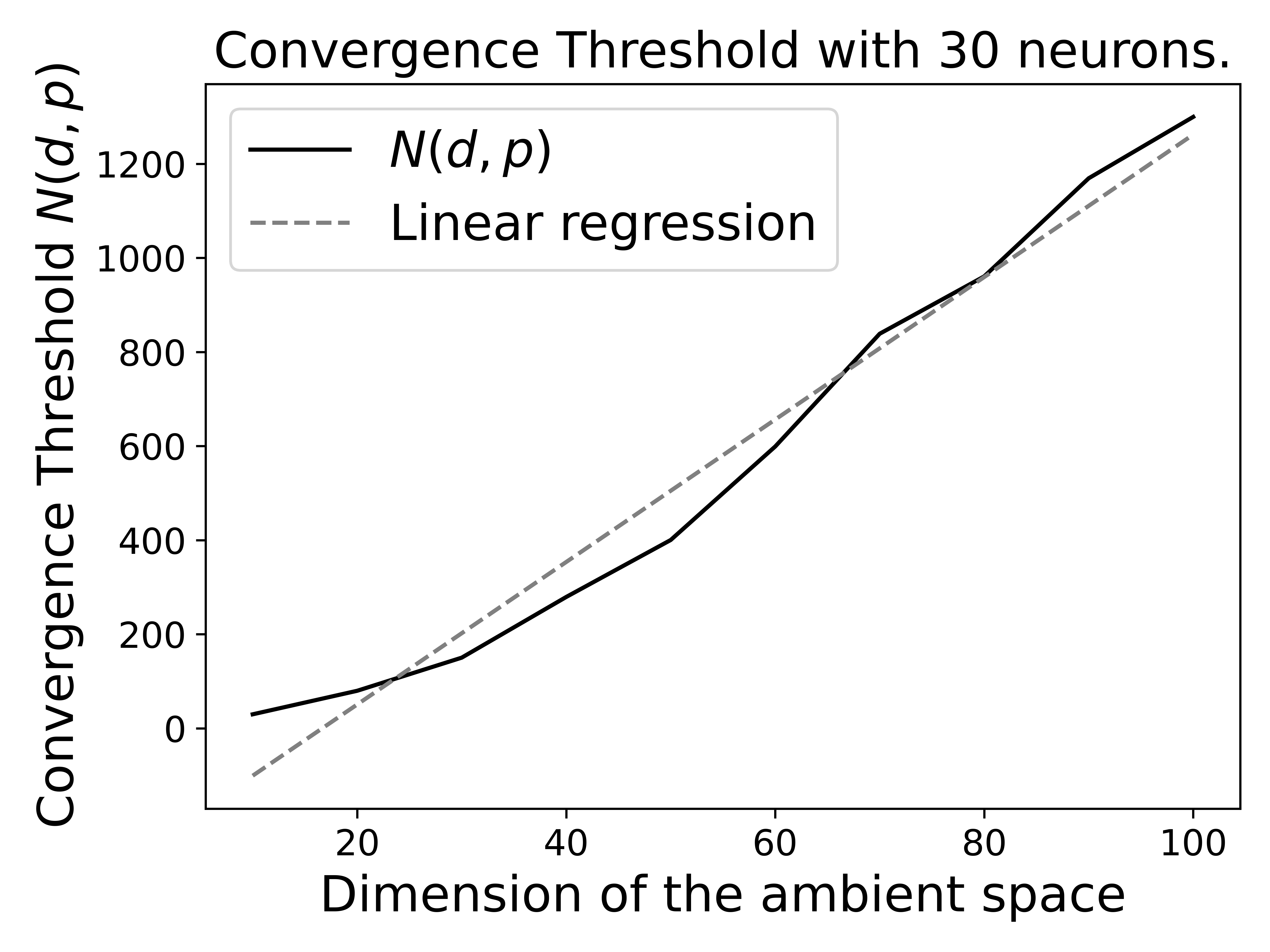
Figure 3: This graph shows the scaling law of the convergence threshold for a fixed number of neurons. It suggests that the scaling is linear in $d$: $N(d,p)=C(p)d$.

Experiment 1.

For the experiment in Figure 2, we trained 500 networks in dimension 100, with $n$ between 2500 and 3500, with 25 runs for each value of $n$. We used $p=\lfloor\frac{\log(\frac{n}{\varepsilon})}{\log(\frac{4}{3})}\rfloor+1$ neurons for each experiment with $\varepsilon=0.05$, since this is the optimal threshold obtained in Lemma 5. We trained the networks with gradient descent using a learning rate of $1$ for a total time $t_{\infty}=1.5\times\frac{\sqrt{np}}{4}\log(np)$ and thus $e=\frac{t_{\infty}}{\text{lr}}$ epochs.

We considered that a network converged as long as its loss went below $\frac{C_{y}^{-}}{2n}$, which then guarantees convergence to 0. We thus early stopped the training and declared the loss was exactly 0. Otherwise, the convergence went for all epochs and the network was assumed to not be able to reach 0 loss. In doted line, we interpolate the probability plot using a sigmoid function, and learned automatically the convergence threshold $N(d,p)$.

For the scaling law on $d$, we fixed $p$ at $30$, and trained networks with dimension varying from 10 to 100, and $n$ ranging from $N(d,p)-15d$ to $N(d,p)+15d$, with step $d$. For each dimension, we interpolate the probability graph using a sigmoid, and plotted the linear trend on Figure 3. For the scaling in $p$, we fixed $d=30$, and varied $p$ from 50 to 400, and plotted the trend on Figure 4 which shows that the scaling in $p$ is sub-linear.

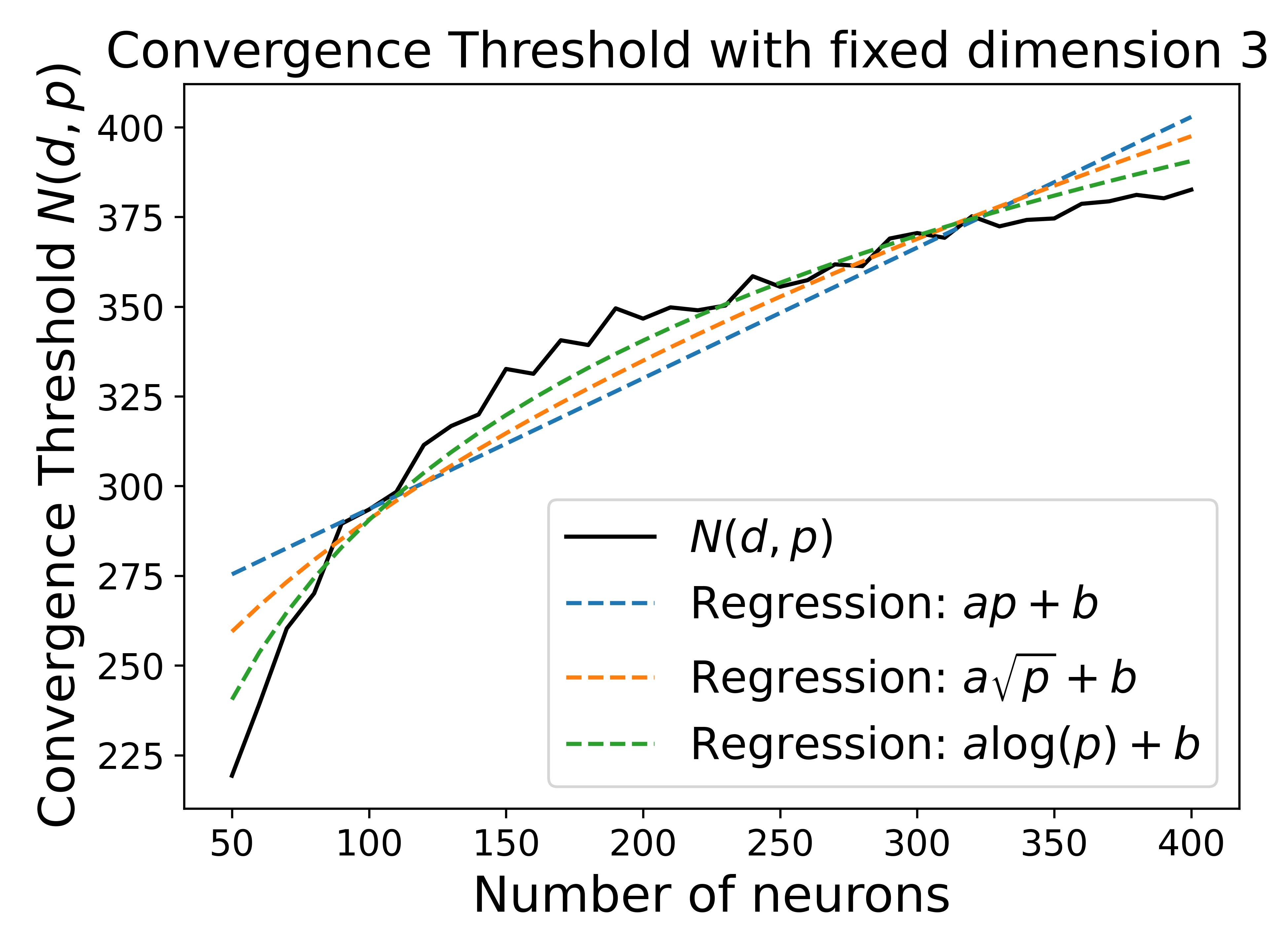
Figure 4: This graph show the scaling law of the convergence threshold for a fixed number of neurons. It suggests that the scaling is not linear in $d$, but it is hard to differentiate between a sub-linear polynomial growth or a logarithmic growth.

Experiment 2.

For this experiment, we trained 500 networks in dimension 2000, with $n$ between 1000 and 2000, with 25 runs for each value of $n$. We used the same number of neurons, learning rates, and epochs as in experiment 1. Let us recall the 4 measures we plotted on the Figure 5:

1. The instantaneous local-PL curvature at the end of the training, $\mu(t_{\infty})=\log\left(\frac{L(t_{\infty}-1)}{L(t_{\infty})}\right)$,

2. The average-PL curvature throughout the training, $\langle\mu_{\infty}\rangle=\log\left(\frac{L(0)}{L(t_{\infty})}\right)$,

3. The lower bound on the local-PL at the end of the training, $\mu_{\text{low}}=\frac{2}{n}\min_{i}\frac{1}{p}\sum_{j=1}^{p}|a_{j}|^{2}1_{j,i}$,

4. The upper bound on the local-PL at the end of the training, $\mu_{\text{upp}}=\frac{16}{n}\max_{i}\frac{1}{p}\sum_{j=1}^{p}|a_{j}|^{2}1_{j,i}$.

Each of the slope being close to $-\frac{1}{2}$, we conclude from this log-log graph that $\langle\mu_{\infty}\rangle=\frac{K}{\sqrt{n}}$ as foreseen in Conjecture 1.

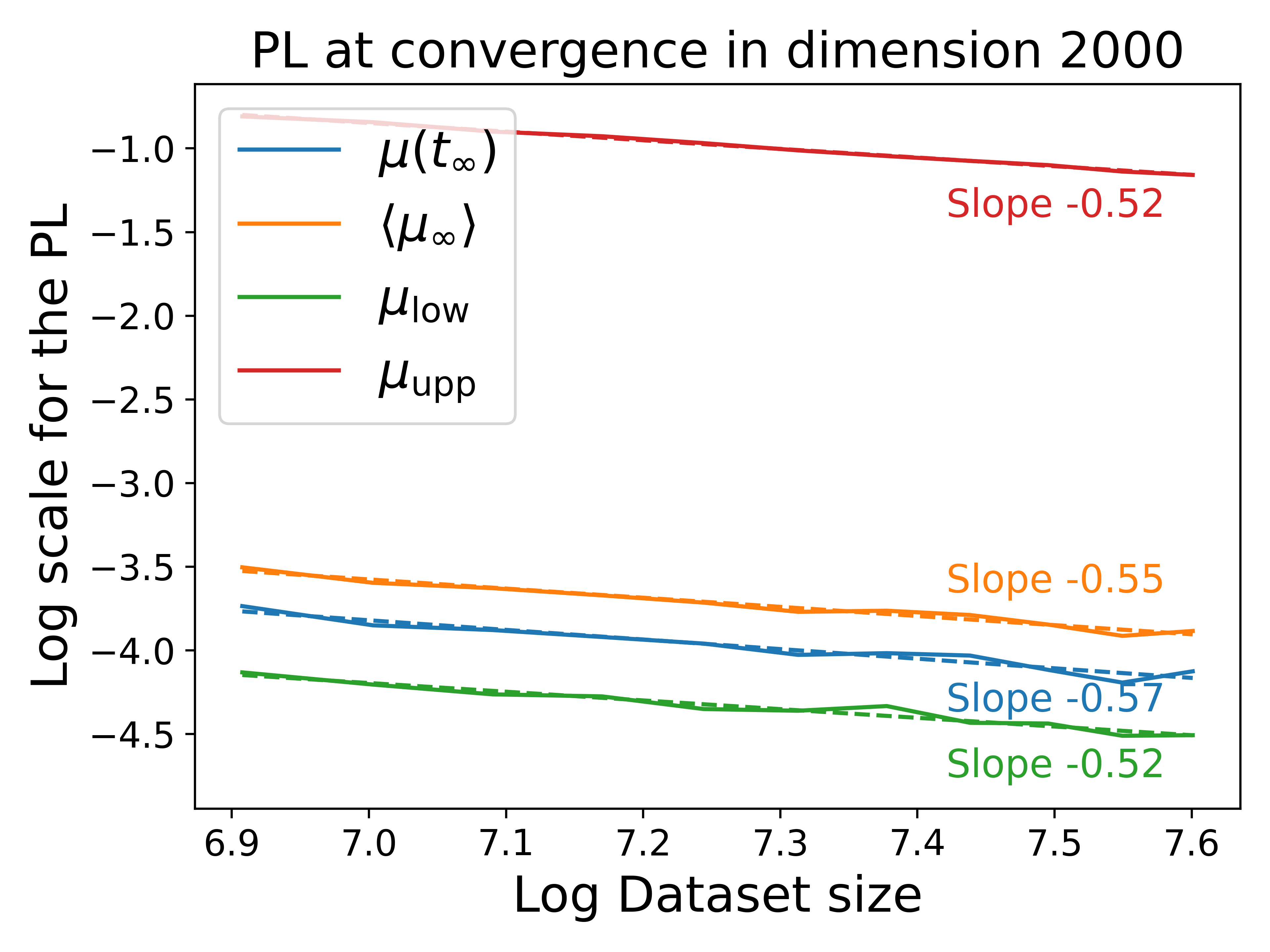
Figure 5: Scaling laws in log-log for different measures of the local-PL curvature in dimension 2000. Each curve is in fact linear with slope close to $-\frac{1}{2}$, which is expected by Conjecture 1.

Each plot’s related experiments were performed on a MacBook Air under 2 hours without acceleration materials.

Appendix C Additional results

C.1 Collapse of the second layer

Similar to the early alignment phenomenon described by Boursier and Flammarion [2024a, b, Theorem 2], where the neurons can rotate and collapse to align on a single vector preventing minimization of the loss, the weights $a_{j}$ of the second layer can also collapse on a single direction. Under the hypothesis that $|a_{j}(0)|\geq||w_{j}(0)||$, the scalar $a_{j}$ cannot change sign, which prevents this scenario in the article’s results. But if $|a_{j}(0)|<||w_{j}(0)||$, they can change sign, and prevent global minimization even when the neurons are correctly initialized. Proposition 3 gives an example of such collapse in low dimension.

Proposition 3.

Suppose that $d=n=p=2$. Let $(x_{1},x_{2})$ be the canonical basis of $\mathbb{R}^{2}$, with the outputs satisfying $y_{1}y_{2}<0,\lambda=|\frac{y_{2}}{y_{1}}|$. Let $|a_{1}(0)|,|a_{2}(0)|\leq\delta$, and let $\min_{j,i}\langle w_{j}(0)|x_{i}\rangle>0$. Then, for $\delta$ small enough, $y_{1}$ large enough, and

$$\sqrt{\max_{j,i}\langle w_{j}(0)|x_{i}\rangle\frac{8}{y_{1}}}\leq\lambda\leq\frac{\min_{j,i}\langle w_{j}(0)|x_{i}\rangle}{\max_{j,i}\langle w_{j}(0)|x_{i}\rangle}$$ (77)

we have $\lim_{t\rightarrow+\infty}L(\theta_{t})>0$.

The proof relies on the ratio between outputs being large $\lambda$, in order to steer the $a_{j}$ to change signs, but not too large to then make the neuron go extinct before the signs of $a_{j}$ may change again. This traps the network in a state of sub-optimal loss, and if $a_{j}$ were initialized as large as the vectors, this collapse could not have happened.

Proof.

of Proposition 3 Without loss of generality, let us suppose $y_{1}>0$ and $y_{2}<0$. We will show that there are values of $\lambda,\varepsilon$ for which the system will not converge. The derivatives of $a_{j}$ at the beginning of the dynamics writes

$$\begin{split}\frac{d}{dt}a_{j}&=\frac{1}{4}(r_{1}\langle w_{j}|x_{1}\rangle+r_{2}\langle w_{j}|x_{2}\rangle)\\ \left|\frac{d}{dt}a_{1}-\frac{y_{1}}{4}(\langle w_{1}|x_{1}\rangle-\lambda\langle w_{1}|x_{2}\rangle)\right|&\leq\max(|a_{1}|,|a_{2}|)\max(||w_{1}||,||w_{2}||)\\ \left|\frac{d}{dt}a_{2}-\frac{y_{1}}{4}(\langle w_{2}|x_{1}\rangle-\lambda\langle w_{2}|x_{2}\rangle)\right|&\leq\max(|a_{1}|,|a_{2}|)\max(||w_{1}||,||w_{2}||)\end{split}$$ (78)

and the derivatives of $\langle w_{j}|x_{i}\rangle$ are

$$\begin{split}\frac{d}{dt}\langle w_{j}|x_{i}\rangle&=\frac{a_{j}r_{i}\mathbb{1}_{j,i}}{2}\\ \left|\frac{d}{dt}\langle w_{j}|x_{1}\rangle-\frac{a_{j}y_{1}\mathbb{1}_{j,1}}{2}\right|&\leq\max(|a_{1}|,|a_{2}|)\max(||w_{1}||,||w_{2}||)\\ \left|\frac{d}{dt}\langle w_{j}|x_{2}\rangle+\lambda\frac{a_{j}y_{2}\mathbb{1}_{j,2}}{2}\right|&\leq\max(|a_{1}|,|a_{2}|)\max(||w_{1}||,||w_{2}||)\\ \end{split}$$ (79)

Now suppose that for $t\leq T$, $|a_{j}|,||w_{j}||\leq M$ and $\langle w_{j}|x_{i}\rangle\geq m>0$, we have

$$\begin{split}a_{j}(t)&\geq-\delta+\left(\frac{y_{1}}{4}(m-\lambda M)-M^{2}\right)t\\ a_{j}(t)&\leq\delta+\left(\frac{y_{1}}{4}(M-\lambda m)+M^{2}\right)t\\ \end{split}$$ (80)

Thus, for $T>\frac{\delta}{\left(\frac{y_{1}}{4}(m-\lambda M)-M^{2}\right)}$ with $\lambda\geq\frac{m}{M}$ and $y_{1}\geq\frac{4M^{2}}{m-\lambda M}$, we have $a_{j}(T)>0$. We now wish to find the constants $M,m$ such that the previous equation will hold. To find the constraint on $m$ and $M$, let us write

$$\begin{split}\langle w_{j}|x_{1}\rangle&\geq\langle w_{j}(0)|x_{1}\rangle-\left(\frac{1}{2}y_{1}M+M^{2}\right)t\\ \langle w_{j}|x_{2}\rangle&\geq\langle w_{j}(0)|x_{2}\rangle-\left(\frac{\lambda}{2}y_{1}M+M^{2}\right)t\\ \langle w_{j}|x_{1}\rangle&\leq\langle w_{j}(0)|x_{1}\rangle+\left(\frac{1}{2}y_{1}M+M^{2}\right)t\\ \langle w_{j}|x_{2}\rangle&\leq\langle w_{j}(0)|x_{2}\rangle+\left(\frac{\lambda}{2}y_{1}M+M^{2}\right)t\\ \end{split}$$ (81)

Thus, the constraints are

$$\begin{split}m&\geq\min\left(\min_{j,i}\langle w_{j}(0)|x_{2}\rangle,\delta\right)-\delta\frac{2y_{1}M+4M^{2}}{y_{1}(m-\lambda M)-4M^{2}}\\ M&\leq\max\left(\max_{j,i}\langle w_{j}(0)|x_{2}\rangle,\delta\right)+\delta\frac{2y_{1}M+4M^{2}}{y_{1}(m-\lambda M)-4M^{2}}\end{split}$$ (82)

We see that the constraint are satisfied with $m\geq\min_{j,i}\langle w_{j}(0)|x_{2}\rangle-2\delta>0$ and $M\leq\max_{j,i}\langle w_{j}(0)|x_{2}\rangle+2\delta$ if: $\delta$ is small enough, $y_{1}$ is large enough, and $\lambda<\frac{\min_{j,i}\langle w_{j}(0)|x_{2}\rangle}{\max_{j,i}\langle w_{j}(0)|x_{2}\rangle}$. Thus, there exists $T>0$ such that at time $T$, we have $a_{1}(T),a_{2}(T)>0$, and no neurons went extinct.

Now, let us show that neurons $\langle w_{j}|x_{2}\rangle$ will go to 0 for some time $\mathcal{T}>0$, while the neurons $a_{j}$ stay positive. We can use the same equations as before, with this time $|a_{j}|,||w_{j}||\leq N$ for $t\leq\mathcal{T}$, and get

$$\langle w_{j}|x_{2}\rangle\leq\langle w_{j}(0)|x_{2}\rangle-\left(\frac{\lambda}{2}y_{1}N-N^{2}\right)t$$ (83)

Thus, for $\mathcal{T}=\frac{2\max_{j}\langle w_{j}(0)|x_{2}\rangle}{\lambda y_{1}N-2N^{2}}$ and $\lambda y_{1}\geq 2N$, we have extinction of the neurons. To find the constraint on $N$, use the bounds on the growth of $a_{j}$ and $\langle w_{j}(0)|x_{1}\rangle$. The constraint is

$$N\leq\max\left(\max_{j}\langle w_{j}(0)|x_{1}\rangle,\delta\right)+2\max_{j}\langle w_{j}(0)|x_{2}\rangle\frac{y_{1}+2N}{\lambda y_{1}-2N}$$ (84)

Thus, the constraints are satisfied with $N\leq\max_{j,i}\langle w_{j}(0)|x_{i}\rangle(1+\frac{3}{\lambda})$ as long as $y_{1}$ is large enough, and

$$\lambda\geq\sqrt{\max_{j,i}\langle w_{j}(0)|x_{i}\rangle\frac{8}{y_{1}}}.$$ (85)

After time $\mathcal{T}$, the neurons $\langle w_{j}(0)|x_{2}\rangle$ went extinct, and thus we have $L(\theta_{t})\geq\frac{y_{2}^{2}}{4}>0$. ∎

C.2 Antipodality

In this section, we give a trick to show how to make the network learn $2d$ vectors in dimension $d$. Indeed, one can see, if $\langle\bar{x}_{i}|\bar{x}_{k}\rangle=-1$, then there is no problem of large interaction between inputs as $1_{j,i}1_{j,k}=0$, since a vector $w_{j}$ is either activated on $x_{i}$ or activated on $x_{k}$. Thus, if we note $\bar{x}_{-i}=-\bar{x}_{i}$, we can replace the condition in Assumption 2, by

$$N_{2}=\left|\left|X^{T}X-\left(\begin{array}[]{c|c}D_{X}^{+}&-\sqrt{D_{X}^{+}D_{X}^{-}}\\ \hline\cr-\sqrt{D_{X}^{+}D_{X}^{-}}&D_{X}^{-}\end{array}\right)\right|\right|\leq\frac{(C_{x}^{-})^{2}}{\sqrt{n}}\frac{C_{y}^{-}}{C_{y}^{+}}$$ (86)

with $D_{X}^{+}$ the diagonal matrix with diagonal terms $||x_{i}||^{2}$, and $D_{X}^{-}$ the diagonal matrix with diagonal terms $||x_{-i}||^{2}$. Thus, adding antipodal vectors will result in the same equations:

$$\begin{split}\frac{d}{dt}\langle w_{j_{i}^{*}}|x_{i}\rangle&\geq\frac{|a_{j_{i}^{*}}|}{n}\left[r_{i}||x_{i}||^{2}1_{{j_{i}^{*}},i}s_{j_{i}^{*}}-r_{-i}||x_{i}||||x_{-i}||1_{{j_{i}^{*}},-i}-N_{2}\sqrt{2nL(\theta(0))}\right]\\ &=\frac{|a_{j_{i}^{*}}|}{n}\left[r_{i}||x_{i}||^{2}1_{{j_{i}^{*}},i}s_{j_{i}^{*}}-N_{2}\sqrt{2nL(\theta(0))}\right]\end{split}$$ (87)

Since, by definition of $j_{i}^{*}$, $\langle w_{j_{i}^{*}}|x_{i}\rangle\geq 0$, thus $1_{{j_{i}^{*}},-i}=0$. And

$$\begin{split}||XP_{j}R||^{2}&\geq(C_{x}^{-})^{2}\left[||P_{j}R||^{2}-2(R^{+}P_{j}^{+})^{T}R^{-}P_{j}^{-}\right]-N_{2}||P_{j}R||^{2}\\ &\geq(C_{x}^{-})^{2}||P_{j}R||^{2}-N_{2}||P_{j}R||^{2}\\ \end{split}$$ (88)

where $R^{+}_{i}=r_{i}$, $R^{-}_{i}=r_{-i}$, $(P_{j}^{+})_{i}=1_{j,i}$ and $(P_{j}^{-})_{i}=1_{j,-i}$. As said $P_{j}^{+}P_{j}^{-}=0$. These two equations being the most important for the proof of Theorem 1, it holds with antipodal input data.

This shows a weakness of the proof: we expect this to generalize when the data are perturbed by $\varepsilon$ small, yet here going from exactly antipodal to nearly-antipodal make the proof incorrect. To accommodate for this, one has to control the small zone were interaction can exists and prevent vectors from entering that zone at all time.

References

- Allen-Zhu et al. [2019] Zeyuan Allen-Zhu, Yuanzhi Li, and Zhao Song. A convergence theory for deep learning via over-parameterization. In International conference on machine learning, pages 242–252, 2019.
- Arora et al. [2019] Sanjeev Arora, Simon Du, Wei Hu, Zhiyuan Li, and Ruosong Wang. Fine-grained analysis of optimization and generalization for overparameterized two-layer neural networks. In International Conference on Machine Learning, pages 322–332, 2019.
- Bach [2024] Francis Bach. Learning Theory from First Principles. MIT Press, 2024.
- Bertoin et al. [2021] David Bertoin, Jérôme Bolte, Sébastien Gerchinovitz, and Edouard Pauwels. Numerical influence of Relu’(0) on backpropagation. Advances in Neural Information Processing Systems, 34:468–479, 2021.
- Bottou et al. [2018] Léon Bottou, Frank E. Curtis, and Jorge Nocedal. Optimization methods for large-scale machine learning. SIAM Review, 60(2):223–311, 2018.
- Boursier and Flammarion [2024a] Etienne Boursier and Nicolas Flammarion. Early alignment in two-layer networks training is a two-edged sword. arXiv preprint arXiv:2401.10791, 2024a.
- Boursier and Flammarion [2024b] Etienne Boursier and Nicolas Flammarion. Simplicity bias and optimization threshold in two-layer relu networks. arXiv preprint arXiv:2410.02348, 2024b.
- Boursier et al. [2022] Etienne Boursier, Loucas Pillaud-Vivien, and Nicolas Flammarion. Gradient flow dynamics of shallow Relu networks for square loss and orthogonal inputs. Advances in Neural Information Processing Systems, 35:20105–20118, 2022.
- Chatterjee [2022] Sourav Chatterjee. Convergence of gradient descent for deep neural networks. arXiv preprint arXiv:2203.16462, 2022.
- Chen et al. [2022] Zhengdao Chen, Eric Vanden-Eijnden, and Joan Bruna. On feature learning in neural networks with global convergence guarantees. International Conference on Learning Representations, 2022.
- Chizat and Bach [2018] Lenaic Chizat and Francis Bach. On the global convergence of gradient descent for over-parameterized models using optimal transport. Advances in Neural Information Processing Systems, 31, 2018.
- Chizat et al. [2019] Lenaic Chizat, Edouard Oyallon, and Francis Bach. On lazy training in differentiable programming. Advances in Neural Information Processing Systems, 32, 2019.
- Du et al. [2019] Simon S. Du, Xiyu Zhai, Barnabas Poczos, and Aarti Singh. Gradient descent provably optimizes over-parameterized neural networks. International Conference on Learning Representations, 2019.
- Frei et al. [2023] Spencer Frei, Gal Vardi, Peter Bartlett, Nathan Srebro, and Wei Hu. Implicit bias in leaky reLU networks trained on high-dimensional data. The Eleventh International Conference on Learning Representations, 2023.
- Gentil [2020] Ivan Gentil. L’entropie, de Clausius aux inégalités fonctionnelles. HAL preprint hal-02464182, 2020.
- Glasgow [2023] Margalit Glasgow. Sgd finds then tunes features in two-layer neural networks with near-optimal sample complexity: A case study in the xor problem. arXiv preprint arXiv:2309.15111, 2023.
- Jacot et al. [2018] Arthur Jacot, Franck Gabriel, and Clément Hongler. Neural tangent kernel: Convergence and generalization in neural networks. Advances in Neural Information Processing Systems, 31, 2018.
- Jentzen and Riekert [2023] Arnulf Jentzen and Adrian Riekert. Convergence analysis for gradient flows in the training of artificial neural networks with Relu activation. Journal of Mathematical Analysis and Applications, 517(2):126601, 2023.
- Ji and Telgarsky [2020] Ziwei Ji and Matus Telgarsky. Directional convergence and alignment in deep learning. Advances in Neural Information Processing Systems, 33:17176–17186, 2020.
- Lee et al. [2016] Jason D. Lee, Max Simchowitz, Michael I. Jordan, and Benjamin Recht. Gradient descent only converges to minimizers. In Conference on learning theory, pages 1246–1257, 2016.
- Liu et al. [2022] Chaoyue Liu, Libin Zhu, and Mikhail Belkin. Loss landscapes and optimization in over-parameterized non-linear systems and neural networks. Applied and Computational Harmonic Analysis, 59:85–116, 2022.
- Lyu and Li [2020] Kaifeng Lyu and Jian Li. Gradient descent maximizes the margin of homogeneous neural networks. International Conference on Learning Representations, 2020.
- Maennel et al. [2018] Hartmut Maennel, Olivier Bousquet, and Sylvain Gelly. Gradient descent quantizes Relu network features. arXiv preprint arXiv:1803.08367, 2018.
- Marcotte et al. [2024] Sibylle Marcotte, Rémi Gribonval, and Gabriel Peyré. Abide by the law and follow the flow: Conservation laws for gradient flows. Advances in Neural Information Processing Systems, 36, 2024.
- Mei et al. [2018] Song Mei, Andrea Montanari, and Phan-Minh Nguyen. A mean field view of the landscape of two-layer neural networks. Proceedings of the National Academy of Sciences, 115(33), 2018.
- Polyak [1964] B. T. Polyak. Gradient methods for solving equations and inequalities. USSR Computational Mathematics and Mathematical Physics, 4(6):17–32, 1964.
- Rotskoff and Vanden-Eijnden [2018] Grant Rotskoff and Eric Vanden-Eijnden. Parameters as interacting particles: long time convergence and asymptotic error scaling of neural networks. Advances in Neural Information Processing Systems, 31, 2018.
- Vershynin [2010] Roman Vershynin. Introduction to the non-asymptotic analysis of random matrices. arXiv preprint arXiv:1011.3027, 2010.
- Wojtowytsch [2020] Stephan Wojtowytsch. On the convergence of gradient descent training for two-layer Relu-networks in the mean field regime. arXiv preprint arXiv:2005.13530, 2020.
- Zhou et al. [2021] Mo Zhou, Rong Ge, and Chi Jin. A local convergence theory for mildly over-parameterized two-layer neural network. In Conference on Learning Theory, pages 4577–4632, 2021.