Napoleonic Constructions in the Hyperbolic Plane
Abstract.
In the Euclidean setting, Napoleon’s Theorem states that if one constructs an equilateral triangle on either the outside or the inside of each side of a given triangle and then connects the barycenters of those three new triangles, the resulting triangle happens to be equilateral.
The case of spherical triangles has been recently shown to be different: on the sphere, besides equilateral triangles, a necessary and sufficient condition for a given triangle to enjoy the above Napoleonic property is that its congruence class should lie on a suitable surface (namely, an ellipsoid in suitable coordinates).
In this article we show that the hyperbolic case is significantly different from both the Euclidean and the spherical setting. Specifically, we establish here that the hyperbolic plane does not admit any Napoleonic triangle, except the equilateral ones. Furthermore, we prove that iterated Napoleonization of any triangle causes it to become smaller and smaller, more and more equilateral and converge to a single point in the limit.
1. Introduction
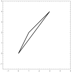
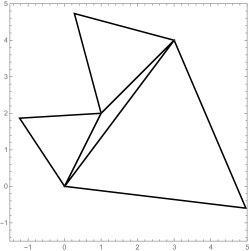
The Napoleonic construction deals with triangles on a surface and proceeds according to the following steps:
-
•
A triangle in a two-dimensional surface is given.
-
•
Three equilateral triangles are constructed on the sides of : namely, one takes points , and on the surface such that the triangles , and are equilateral (two different constructions arise, according to the direction chosen for the points , and ).
-
•
The centroids (i.e. barycenters) , and of the equilateral triangles , and are considered and the triangle is called the Napoleonization of .
-
•
If the Napoleonization is an equilateral triangle, then the initial triangle is called Napoleonic.
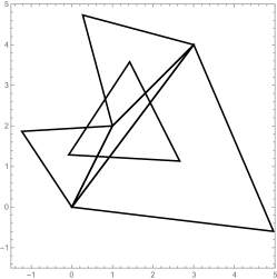
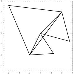
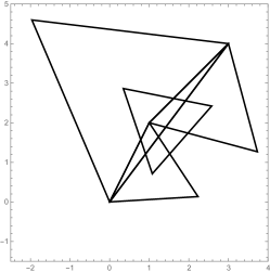
The classical case of this construction occurs when the ambient surface is the Euclidean plane. In this situation, all triangles are Napoleonic: this is a famous result going under the name of Napoleon’s Theorem: see e.g. [MR2928662] and the references therein for the fascinating history of this result (see also Figures 1.1 and 1.2 for a sketch of the Napoleonic constructions in the Euclidean plane).
In the Euclidean case, Napoleon’s Theorem attracted the attention of several first-rate mathematicians, including Fields Medallist Jesse Douglas; in fact, the question of extending Napoleon’s Theorem from planar triangles to polygons is known as the Petr-Douglas-Neumann problem, see [zbMATH02641104, MR2178, MR6839]. Napoleon’s Theorem also finds practical applications in some optimization questions, such as the Fermat-Steiner-Torricelli problem, see [MR4298718].
Among the many modern extensions of Napoleon’s Theorem, a natural field of investigation is the discovery and classification of Napoleonic triangles in ambient surfaces different from the Euclidean plane. This happens to be a rather difficult problem about which little is known.
So far, the only ambient manifold for which all Napoleonic triangles have been classified is the round sphere. Specifically, in [MR4727700] it is established that if a spherical triangle is Napoleonic then either it is equilateral or its congruency class lies in an explicit surfaces, which, in an appropriate coordinate system, can be written as a two-dimensional rotational ellipsoid (and, conversely, all congruency classes in this ellipsoid correspond to Napoleonic triangles). What is more, all non-equilateral Napoleonic triangles on the sphere produce congruent Napoleonizations.
The case of Napoleonic constructions in the hyperbolic plane appears then as a natural question. So far, to the best of our knowledge, the only available results in this setting go back to [MR1847491] and deal with an infinite sequence of recursively defined hyperbolic triangles (as explicitly mentioned in [MRev] this construction is inspired by Napoleon’s Theorem, but structurally quite different from it). In particular, no specific investigation of Napoleonic constructions in the hyperbolic plane has been carried out till now.
The goal of this paper is to fill this gap. For concreteness, as a model for the hyperbolic plane we consider here the upper sheet of the unit hyperboloid in the Minkowski space (see Section 2 for details). Our first result states that the only Napoleonic triangles are the trivial ones (i.e., the ones for which the initial triangle was equilateral):
Theorem 1.1.
If the Napoleonization of a hyperbolic triangle is equilateral, then the initial triangle is equilateral too.
We stress that the hyperbolic case dealt with in Theorem 1.1 is surprisingly different both from the Euclidean case (in which all Napoleonizations are equilateral) and the spherical case (in which an ellipsoid of parameters produces non-trivial cases of equilateral Napoleonizations). We believe that the structural differences of Napoleon-like results depending on the geometry of the ambient surface is indeed a noteworthy phenomenon and a brand-new line of investigation which deserves a deeper understanding.
Another question of interest in this setting is what happens after repeated Napoleonizations, i.e. by taking a hyperbolic triangle to start with, and applying the Napoleonic construction over and over. For that target, given a hyperbolic triangle , we denote its Napoleonization by , and recursively we set to be the Napoleonization of . In this framework, our result goes as follows:
Theorem 1.2.
As increases, the triangles become smaller, more nearly equilateral and, as , more nearly a single point.
We point out that Theorem 1.2 is in sharp contrast with the Euclidean case (flat triangles remain equilateral and do not contract under repeated Napoleonizations, actually they just rotate by , up to relabeling vertices). The comparison with the Euclidean case also highlights an unavoidable difficulty intrinsically linked to the proof of Theorem 1.2: indeed, if repeated Napoleonizations tend to approach a point, the setting becomes “more and more Euclidean” during the iteration, thus making the convergence to a point problematic precisely when we approach the limit.
The rest of the paper is organized as follows. In Section 2 we gather some preliminary observations on the hyperboloid model and the hyperbolic triangles. In Section 3 we introduce a bespoke set of hyperbolic coordinates, which are different from the standard hyperbolic distance and come in handy to simplify several otherwise cumbersome calculations. Sections 4 and 5 contain the proofs of Theorems 1.1 and 1.2, respectively.
2. Preliminaries on the Hyperboloid Model and the Hyperbolic Triangles
We recall that the Minkowski inner product on is given by
Equivalently
where denotes the Euclidean inner product and is the diagonal matrix
The (upper unit) hyperboloid is
where is the timelike vector . Moreover, we denote by and .
As customary111For an elementary proof of (2.1), one can write and , with , and , , and use the standard Cauchy-Schwarz inequality. Indeed, we note that, for all , , Also, choosing and , we see that , and similarly , yielding that and and that Consequently, and . Thus, since the classical inequality in (2.1) plainly follows (and actually, tracing the equality cases in the above inequality, one also gets that equality in (2.1) holds if and only if ). we observe that if , , then,
| (2.1) |
The hyperbolic cross-product of vectors in Minkowski space is given by
where is the Euclidean cross-product.
Since is orthogonal with determinant , we deduce from the formula
that, for any , , , ,
Therefore, using the Binet-Cauchy Identity,
| (2.2) |
The hyperbolic scalar triple product of , , is also the Euclidean scalar triple product , so it has the same symmetries.
Given two points on the hyperboloid, a third point can be written as a combination of these two points and their cross-product. More explicitly, we have that:
Lemma 2.1.
Let . Then, any can be written in the form
| (2.3) |
with
| (2.4) |
Also,
| (2.5) |
Proof.
The case of isosceles and equilateral triangles on the hyperboloid are particular cases of Lemma 2.1 and go as follows:
Corollary 2.3.
Let be equilateral with .
Then,
with .
Proof.
We now reconsider Corollary 2.3 with the aim of identifying the centroid of an equilateral triangle on the unit hyperboloid (where, by definition, the centroid of a triangle is the sum of the coordinates of its vertices projected over the hyperboloid):
Lemma 2.4.
Let be equilateral with . Let be its centroid.
Then,
with .
Proof.
The centroid of the equilateral hyperbolic triangle is , where
and, thanks to the equality in (2.2),
The desired result now plainly follows. ∎
3. A Bespoke Set of Hyperbolic Coordinates
From now on we consider three distinct points , , and define
| (3.1) |
and
| (3.2) |
We stress that is symmetric with respect to permutations of , and , and that is symmetric with respect to cyclic permutations.
Since Theorems 1.1 and 1.2 are invariant under permutations of , and , we can list the vertices , and so that
| (3.3) |
This reordering of vertices will be implicitly assumed in what follows.
From now on, we will also consider , such that and are equilateral. Let also be the centroid of and be the centroid of .
With this notation, we can take a step further from Lemma 2.4 and obtain that:
Lemma 3.1.
We have that
with , .
Proof.
We now introduce a new set of “hyperbolic units of measurements”, technically and conceptually different from the standard hyperbolic distance , which come in handy to simplify several otherwise cumbersome calculations. Namely, we define
| (3.4) |
We point out that defines the congruency class of the hyperbolic triangle, and that these hyperbolic coordinates are well defined, thanks to (2.1).
The main features of these hyperbolic coordinates are the following:
Lemma 3.2.
For all , we have that
| (3.5) |
and
| (3.6) |
Proof.
Also, by the triangle inequality in (see e.g. page 70 in [MR1205776]), for ,
We recall that
Therefore, using this formula with and , we find that
from which one obtains (3.6). ∎
Now we calculate and :
Proposition 3.3.
We have that
| (3.7) |
and
| (3.8) |
Proof.
Moreover, by (2.5),
Now we define
| (3.9) |
and we have the following two estimates:
Lemma 3.4.
It holds that
| (3.10) | |||||
| (3.11) | and |
4. Napoleonic Triangles and Proof of Theorem 1.1
From now on, we suppose that , and are not cogeodesic, namely . Hence, by (3.3),
Set also222Because of these choices, if then . Similarly, if then , and if then . Our attention is not limited to the case where is isosceles. .
Lemma 4.1.
We have that, for ,
| (4.1) |
and
| (4.2) |
Proof.
Using Lemma 2.4 we write that
Therefore, recalling also the definitions in (3.1), (3.2) and (3.4) and exploiting (2.2),
| (4.3) |
Corollary 4.2.
Suppose that is not equilateral.
Then, is equilateral if and only if
| (4.4) |
Proof.
With this preliminary work, we can now complete the proof of the non-existence of non-trivial Napoleonic triangles in the hyperbolic plane.
Proof of Theorem 1.1.
Suppose that is Napoleonic, i.e. is equilateral. If is not equilateral then (4.4) implies that
| (4.5) |
with and given by (3.7) and (3.8) as symmetric polynomials in , and . After these substitutions, one sees that the left-hand side of (4.5) is
that in turn equals to
which is strictly positive.
Accordingly, we have that must be equilateral. In conclusion, all Napoleonic triangles in are equilateral, as claimed. ∎
5. Napoleonic Progressions and proof of Theorem 1.2
From now on, we deal with repeated Napoleonization. For this purpose, we use the notation introduced in Section 3 and, after a cyclic relabelling, we can suppose that
| (5.1) |
For , we let
| (5.2) |
We remark that are well defined, in light of (2.1) and the fact that , .
We also define
and
| (5.3) |
We point out that, with this notation, equation (4.2) reads as
| (5.4) |
Moreover, we observe that for , we have that . Therefore, in this case, , and are in the same order as , and .
The main calculation needed to understand repeated Napoleonization is as follows:
Proposition 5.1.
We have that
| (5.5) |
Proof.
Applying the Cauchy-Schwarz inequality to the vectors and , we see that
This observation and (3.11) give that
| (5.6) |
For our purposes, Proposition 5.1 is important, since it shows that repeated Napoleonization, with , gives a sequence of hyperbolic triangles, with geometrically decreasing differences of lengths of sides. This allows us to complete the proof of Theorem 1.2: in this respect, we distinguish the contractive iterations when and when .
Proof of Theorem 1.2 when .
We also observe that, recalling (3.7),
| (5.8) |
Now we set and we claim that
| (5.9) |
Indeed, if then, in light of (3.5), we have that for all and so also the left-hand side of (5.9) equals zero. Therefore, in this case we are done. Hence, from now on we suppose that .
Consequently, setting , we find that
| (5.11) |
Thus, for the hyperbolic triangles satisfy
In particular, for ,
establishing the desired result.∎
Proof of Theorem 1.2 when .
For , we have that . Accordingly, without loss of generality, we may suppose that , where , with and .
Also, we claim that
| (5.14) |
Indeed, if , then (3.5) and (5.1) give that also , and so the left-hand side of (5.14) vanishes as well, thus establishing the desidered inequality.
If instead , we recall (5.1) and we see that
which implies the desired inequality in (5.14) in this case as well.
From (5.13) and (5.14), and recalling also (5.1), we thereby conclude that
This and (5.12) entail that
| (5.15) |
Now, writing
we have that
With this notation, we deduce from (5.4) and (5.5) that
| (5.16) |
where is independent of , and also independent of .
Moreover (5.15) becomes
| (5.17) |
By (5.16), we can choose so large that
In this way, we see that, for all ,
Hence, by this and (5.17), for ,
namely is an upper bound for the sequence .
We will now iterate this argument as follows. For , suppose that we have and an upper bound for the sequence for some . Notice that, in light of (5.17), the upper bound . Suppose also that if , and otherwise.
If , set , and .
If instead , by (5.16), we can choose so large that
and we stress that the right hand side is positive because .
Also,
| (5.18) |
We point out that, from the definition of , we have that , and thus . We conclude that the sequence of upper bounds is nonincreasing and bounded below by , and accordingly the following limit exists:
with .
Hence, for , we have that
namely
yielding the desired result. ∎
Acknowledgements
This work has been supported by the Australian Future Fellowship FT230100333 and by the Australian Laureate Fellowship FL190100081.
References
- \ProcessBibTeXEntry \ProcessBibTeXEntry \ProcessBibTeXEntry \ProcessBibTeXEntry \ProcessBibTeXEntry \ProcessBibTeXEntry \ProcessBibTeXEntry \ProcessBibTeXEntry \ProcessBibTeXEntry