Deviations from Random Matrix Theory in quantum chaotic systems: A Perspective from Observable Properties
Abstract
In this paper we study deviations from random matrix theory (RMT) in quantum chaotic systems from a perspective of observable properties. Specifically, we focus on the envelope function of the off-diagonal elements of few-body observables written in the eigenbasis of a quantum chaotic many-body system, as introduced in the eigenstate thermalization hypothesis ansatz. Our objective is to understand the origin of the nontrivial structure of the envelope function in real systems and its connection to the distance of the system from a fully random system described by RMT. To this end, we introduce a method to systematically induce randomness into a real model, which eventually transitions into a random matrix model. Our numerical simulations of a defect Ising model show that the nontrivial structure of the envelope function of local spins becomes less pronounced as the randomness of the system increase, eventually disappearing when the system becomes fully random. Our results imply that the structure of the envelope function of few-body observables is closely related to the randomness of the system, which can be used to characterize the deviation from random matrix theory.
I Introduction
What is the most intuitive perception of chaotic motion? For most individuals, the answer likely involves envisioning chaotic motion as a type of movement resulting from intricate interactions characterized by significant disorder and randomness [1].
In quantum systems, the similarity of statistical properties to random matrix theory (RMT) has long been used as indicator of quantum chaos. For instance, quantum chaotic systems possess an energy spectrum with fluctuations universally described by RMT [2, 3, 4, 5, 1, 6, 7, 8, 9]. It has also been shown that eigenstates of quantum chaotic systems also exhibit universal properties, with their components in certain basis following Gaussian distribution [10, 11, 12, 13, 14, 15, 16], in consistence with RMT.
However, despite the similarity in fluctuation properties described above, quantum chaotic systems deviate from fully random systems described by RMT in various ways. It is known that, average properties, such as averaged spectral density and averaged shape of eigenfunctions (in fixed basis) are usually system-dependent and non-universal, which deviates from RMT. It is natural to ask whether and how the similarity and deviation from RMT are reflected in the properties of observables.
To address this question, we recall the well-known Eigenstate Thermalization Hypothesis (ETH) [17, 18, 19, 20, 21, 22, 23, 24, 25, 26], which make assumptions on the matrix elements of few-body observable in the eigenbasis of the system’s Hamiltonian . The ETH ansatz conjectures that
| (1) |
where and denote the eigenvalue and eigenstate of , respectively. and are smooth functions of their arguments, is the Kronecker Delta function, and are random variables with a normal distribution (zero mean and unit variance). Although ETH remains a hypothesis due to the lack of rigorous proof, most aspects of the ETH have been validated through numerical simulations [17, 25, 27, 28, 29, 30, 31, 32]. It is now widely accepted that the ETH holds for quantum chaotic systems when considering few-body observables.
According to ETH ansatz, the fluctuation term are universal and inline with RMT. In contrast, the envelope function of the diagonal and off-diagonal part, and typically depends on the specific system. In this paper, we show that the correlation between eigenstate and the considering observable play an crucial role in the structure of envelope function . Furthermore, we introduce a systematically way to induce randomness into a real system, disrupts these correlations, gradually transitions the system to a fully random one. With this method, we show numerically how the envelope function as the system becomes more “random”. Our results indicate that the structure of is closely related to the randomness of the system, and can be used as an indicator of deviations from RMT in quantum chaotic systems.
The rest of the paper is organized as follows. In Sec.II, we present examples illustrating the shape of the envelope function . In Sec.III, we explore the relationship between the correlations in energy functions and the behavior of . In Section IV, we use the behavior of as a tool to illustrate how increasing randomness of the model disrupts correlations. Finally, in Sec.V, we provide conclusions and some discussions.
II Envelope function at a glance
We begin by presenting examples of the envelope function . In the following, the eigenstates and eigenvalues of Hamiltonian are denoted by and , respectively:
| (2) |
According to the definition in Eq.(1), the envelope function can be obtained by averaging the off-diagonal elements of the matrix :
| (3) |
where , and the average is taken over narrow energy shells around and . In the specific numerical calculations that follow, each energy shell contains approximately 15 levels around and .
As our first model, we consider the defect Ising chain (DIS), which consists of -spins subjected to an inhomogeneous transverse field. The Hamiltonian is given by:
| (4) |
where are Pauli matrices at site , and the parameters are set as , , , and . The number of spins in the system is . Under these parameters, the system is chaotic.111 The chaocity of the model is shown in Appendix A.
Fig.1 shows as a function of for the observable . For clearer insight, we show a cross-section for fixed in the inset of Fig.1. It is evident that there is a slowly changing plateau at small energy differences , followed by an exponential decay at large .
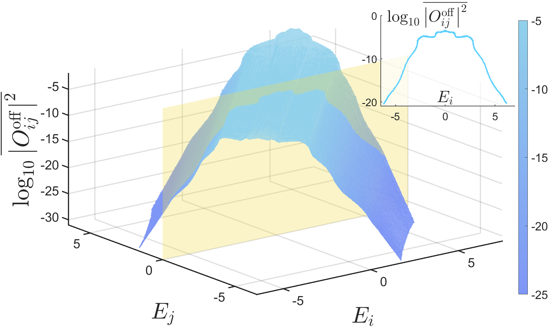
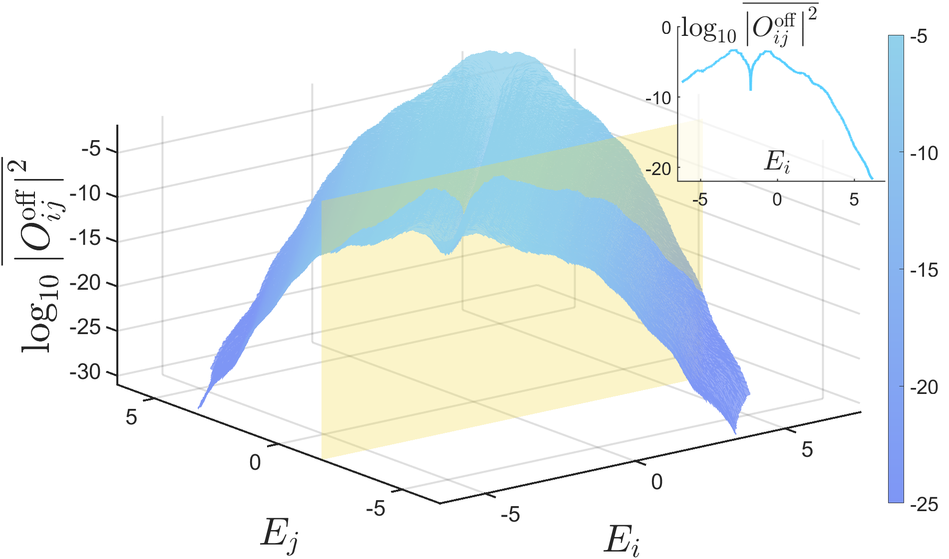
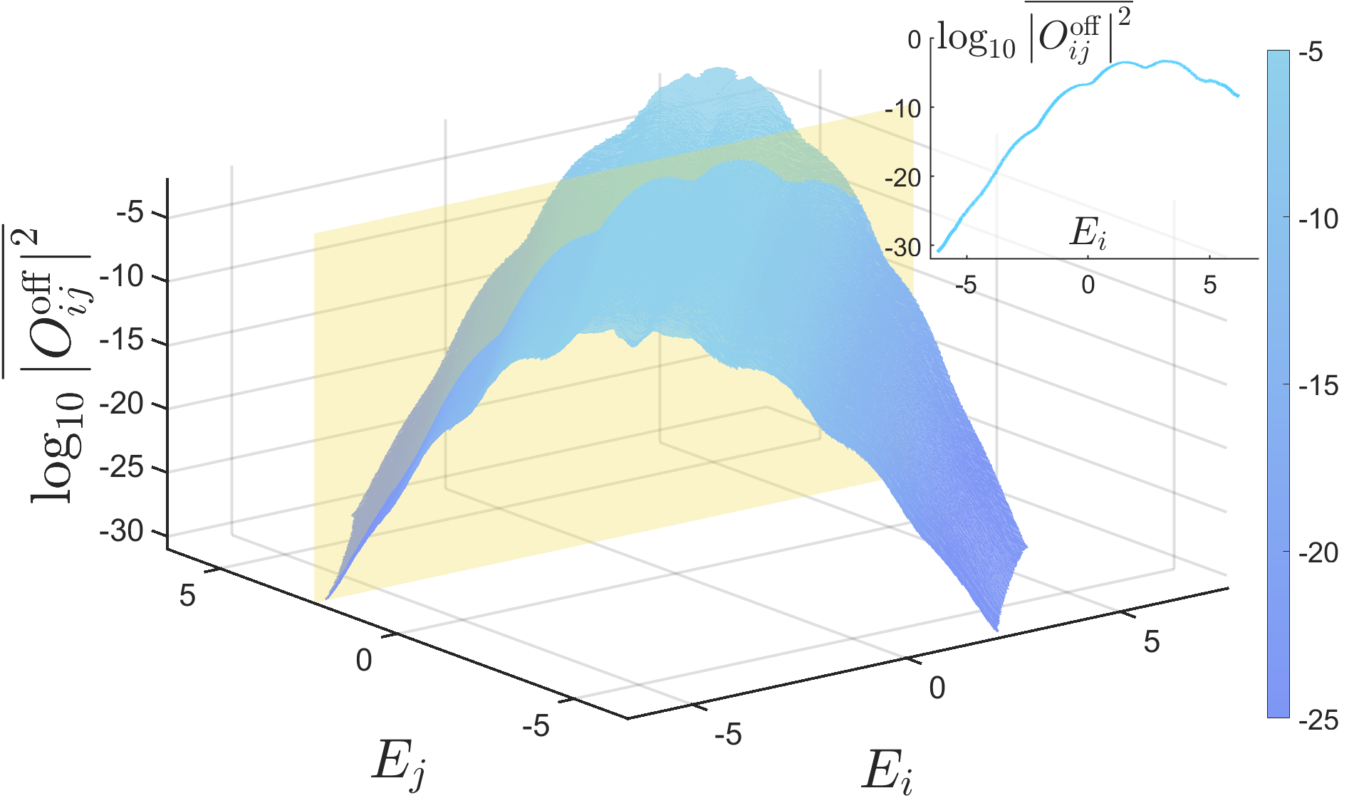
A slowly changing plateau at small followed by exponential decay at large is a typical behavior of the function for common quantum chaotic systems. Fig.2 and Fig.3 show the functions for the observables and , respectively, exhibiting similar behavior. Additionally, such behavior has been observed in other quantum chaotic systems [33].
In addition to the defect Ising model discussed above, which contains only a few parameters, we also study a fully random model whose Hamiltonian is drawn from the Gaussian Orthogonal Ensemble (GOE) random matrix ensemble. Here, we consider an operator , whose matrix elements are, in form, congruent to those of the Pauli operator . This congruence is observed within a representation characterized by the matrix elements of being exclusively Gaussian random numbers. The envelope function in this case is shown in Fig.4.
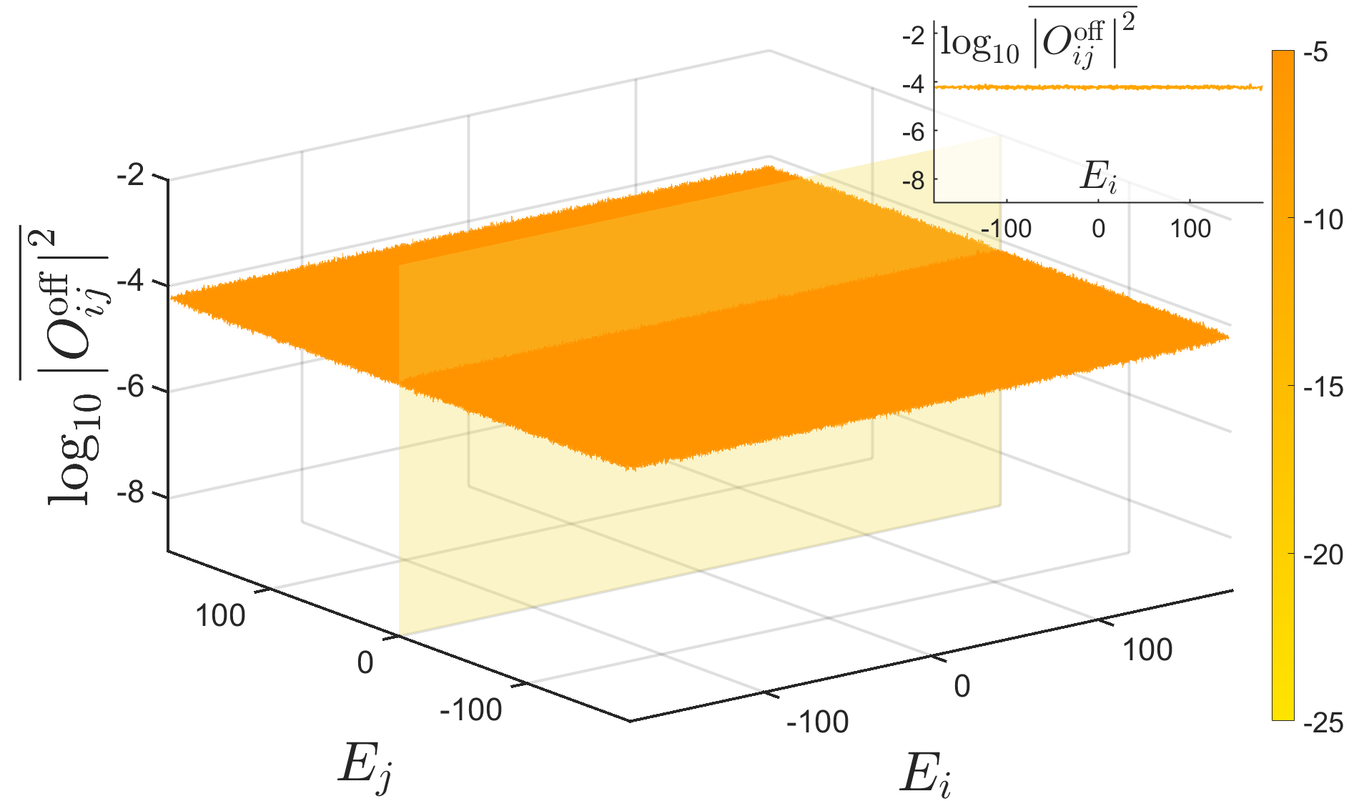
From Fig.4, we observe that, unlike the DIS model, the function in the random matrix model is flat, and the exponential decay at large is absent. This provides the first indication in this paper that randomness in the model disrupts the fast exponential decay of the function.
III Exponential Decay and Correlations
In this section, we elucidate the connection between the exponential decay of at large and the correlations between eigenstates and the observable.
To this end, We expand the energy eigenstates of the DIS model on the uncoupled basis 222 The precise definition of can be found in Appendix A (which is also the eigenbasis of the observable of interest ) as follows:
| (5) |
where are complex numbers, with their magnitudes denoted by and phases denoted by :
| (6) |
Utilizing the expansion outlined in Eq.(5), we can construct a set of ”randomized wavefunctions of the DIS model,” denoted by . These are generated by substituting in Eq.(6) with independent random numbers drawn from a uniform distribution:
| (7) |
This operation preserves the magnitude of the eigenfunction while disrupting the phase correlations among the components of the wavefunctions manually.
For simplicity, in this paper, we consider only real wavefunctions. In this case, are randomly chosen from , or equivalently, are randomly selected from .
Based on this construction, we calculate the matrix elements , where is again taken as . A cross-section of the results is plotted in Fig.5 (yellow line).
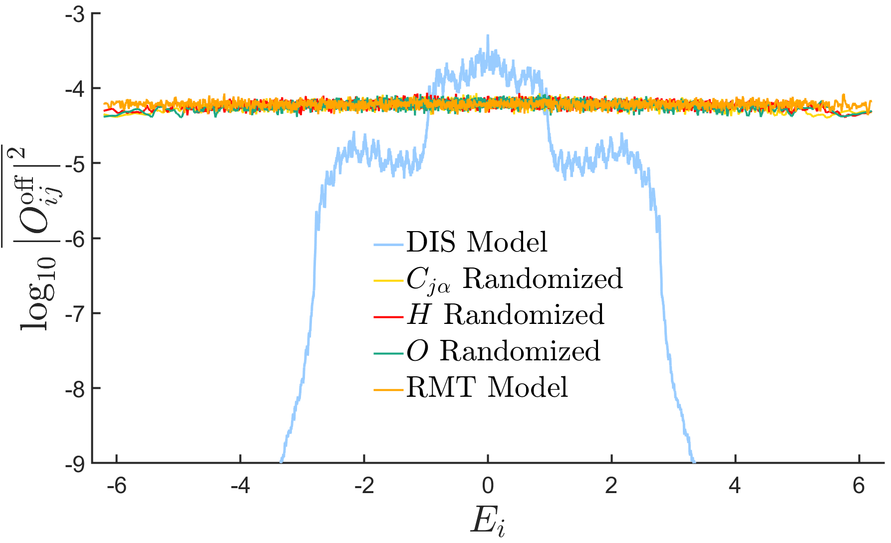
Figure 5 shows that, in , the exponential decay at large disappears, and the function becomes similar to the result predicted by the random matrix model. This finding indicates that the correlations among the phases of the original eigenfunctions of the DIS model are crucial for maintaining the exponential decay of the function. When these correlations are destroyed, the function becomes structureless.
It is worth noting that not just GOE random matrix Hamiltonian can produce eigenstates with disruption of correlations sufficient to flatten the function. The red line in Fig.5 shows the of another system, where the observable is again taken as , but the Hamiltonian is randomized from the original Hamiltonian of the DIS model. Specifically, the randomized Hamiltonian is generated by the following method:
| (8) |
where are independent random numbers drawn from a Gaussian distribution. This operation retains all zero elements of the matrix , and the average magnitudes of are equal to . In other words, the main structural features of are preserved. Moreover, since the original Hamiltonian of the DIS model is a sparse matrix in the representation, the number of random parameters contained in is much less than that in a GOE random matrix. However, despite retaining the main structural features of and containing far fewer random parameters than a GOE random matrix, Fig.5 shows that these random parameters are still enough to disrupt the correlations between eigenstates and observables and further flatten the function.
Besides the conditions discussed above, we would also like to point out that randomization of the observable can also flatten the function. The green line in Fig.5 shows the shape of , where is the energy eigenstate of the original DIS model, and the randomized observable is constructed as follows:
| (9) |
The are also independent random numbers drawn from a Gaussian distribution. From Fig.5, we can see that in this case, the behavior of the function is again close to that in the random matrix model but far from the rapid decay behavior in the original DIS model.
As a short summary of this section, we show numerically that, correlation between eigenstates and observables are crucial for the non-trivial structure of the envelope function . becomes flat (structureless) once such correlations are destroyed.
IV Disruption of Correlations through Enhanced Randomness
The preceding section illustrated that correlations in the energy eigenfunctions of quantum chaotic systems lead to an exponential decay of for large , while a flat indicates uncorrelatedness between eigenstates of Hamiltonian and considered observable. Leveraging this strong connection between the behavior of and the correlations in energy eigenfunctions, the behavior of can be utilized as a tool for quantifying the strength of these correlations.
In this section, we will employ this tool to observe the destructive process of correlations due to the increase of parameters in the model.
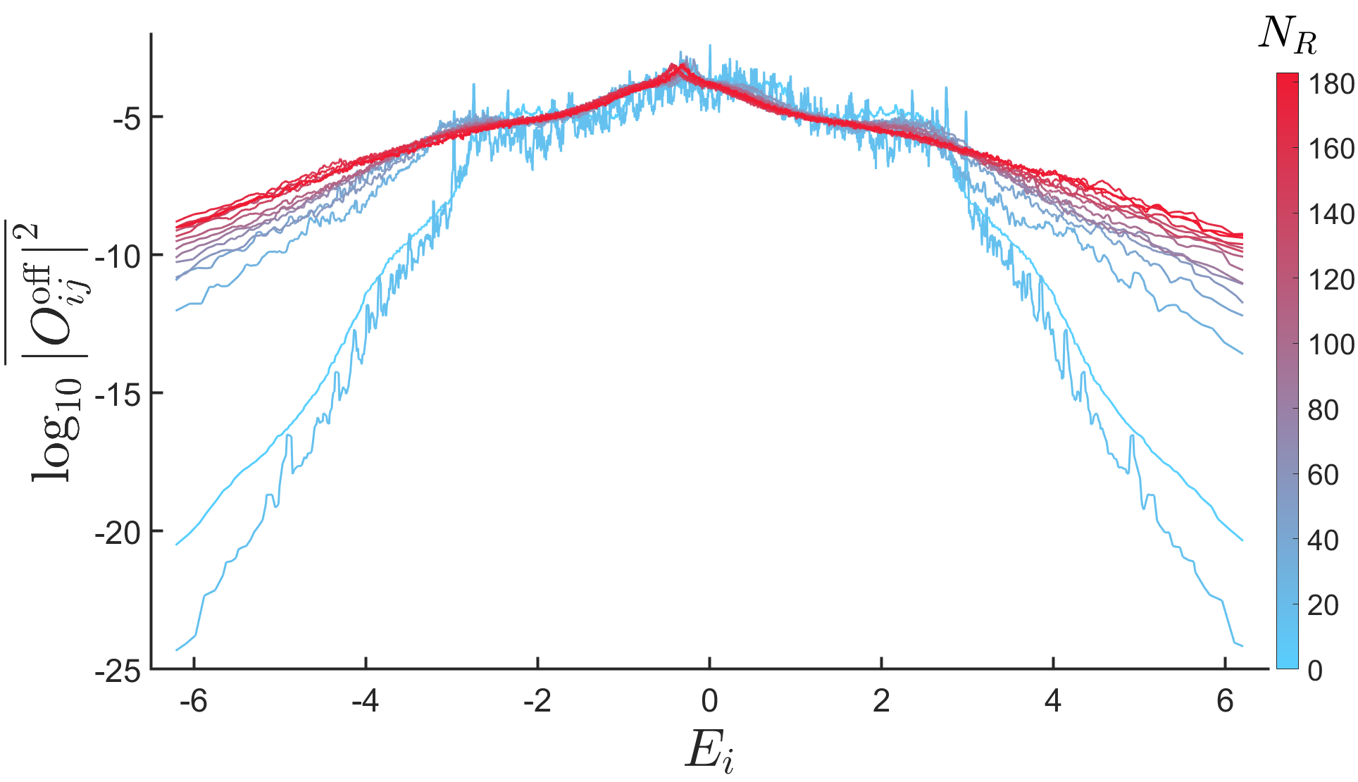
Fig.6 depicts the behavior of as more and more random parameters are introduced into the Hamiltonian of the original DIS model. The method for adding random parameters is detailed in Appendix B. The observable is consistently set as across all scenarios.
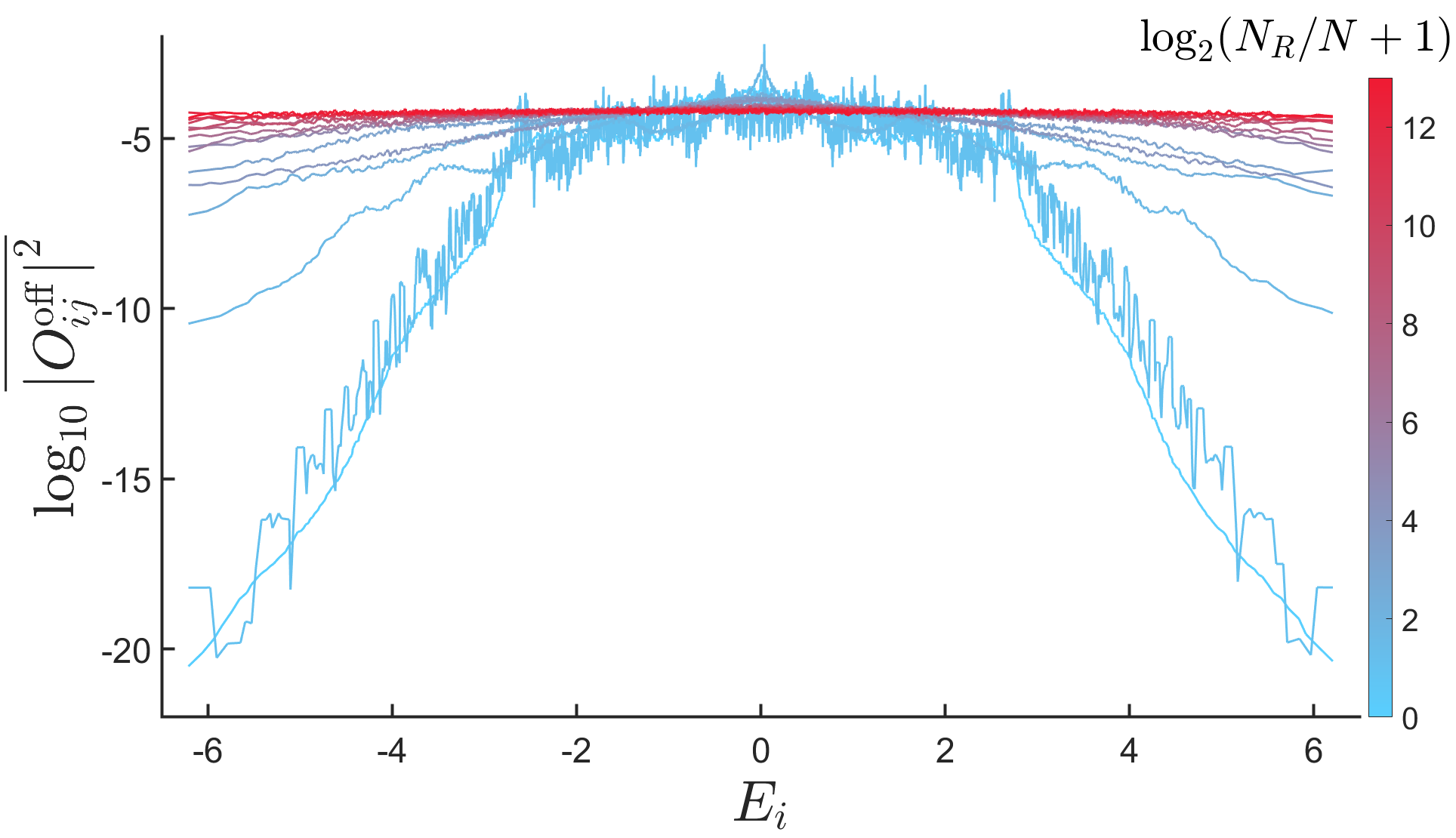
As observed in Fig.6, the increase in the number of random parameters leads to a progressively flatter function. This trend signifies that the growing number of random parameters gradually disrupts the correlations between the energy states and observables. Additionally, Appendix C presents a similar analysis of the variation in functions. when random parameters are introduced into the Hamiltonian of the original DIS model using an alternative method, analogous phenomena is observed (Fig.9).
V Discussions and Conclusions
In this paper, we have explored the relationship between randomness of system and the structure of envelope function of few-body observables. We have shown that, correlations between eigenstates of the system and the considered observables is essential for in the emergence of non-trivial structure of . Introducing a systematically way to induce randomness into a real system, we find numerically that such non-trivial structure gradually become less pronounced. and eventually disappears when the system is fully random. Furthermore, our results suggest that non-trivial structure of can serve as an indicator of the deviations from RMT in real quantum chaotic systems.
A natural question would be to study quantitatively the relation between randomness of the system and the non-trivialness of the structure of . It would also interesting to consider higher-order envelope function introduced in the so-called general ETH [34, 35].
Acknowledgements.
This work was partially supported by the Natural Science Foundation of China under Grant Nos. 12175222, 11535011, and 11775210. J.W. acknowledges support from Deutsche Forschungsgemeinschaft (DFG), under Grant No. 531128043, and under Grant No. 397107022, No. 397067869, and No. 397082825, within the DFG Research Unit FOR 2692, under Grant No. 355031190.Appendix A Chaocity of the model
Let the uncoupled basis of -spins be denoted by , which represents the common eigenstate of all . For instance, one such can be expressed as:
| (10) |
where and are eigenstates of .
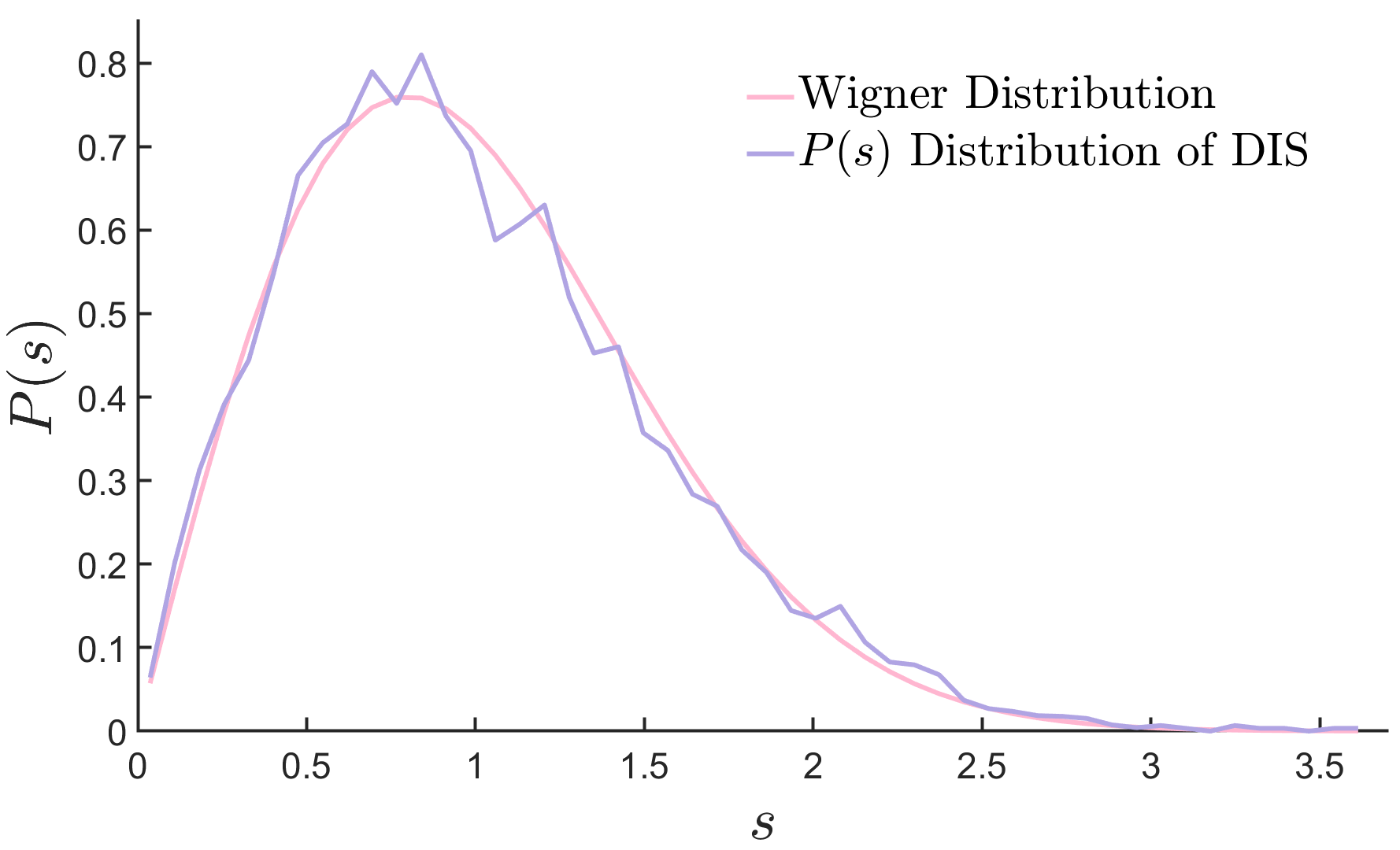
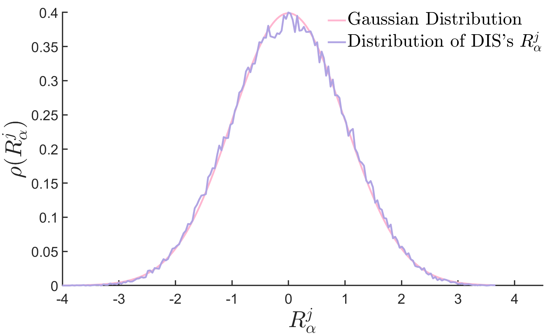
To check the chaocity of the system, we examine in Fig.7 the distribution of the nearest level spacing. A good agreement with the Wigner-Dyson distribution (as predicted by Random Matrix Theory [1]) is observed, indicating that the system behaves chaotically. Additionally, we present the distribution of the rescaled components of the eigenfunctions in the uncoupled basis . A good agreement with the Gaussian distribution asserted by Berry’s conjecture [10, 11] is also evident (Fig.8).
Appendix B A Method to Add Random Parameters into the DIS Model
Consider the Hamiltonian of the DIS model:
| (11) |
In the representation, the first term contains only off-diagonal elements, while the other terms contain only diagonal elements.
Our goal is to introduce more independent parameters into the off-diagonal part of the Hamiltonian in Eq.(11), specifically by adding more independent parameters to the first term. We aim to do this while maintaining the structure of the Hamiltonian matrix as much as possible and ensuring that the new parameters are physically meaningful.
To achieve this, we start by multiplying each coefficient before in the first term by an independent random number. This changes the first term as follows:
| (12) |
where , and are independent Gaussian random numbers with an average value of either or evenly. This operation increases the number of independent parameters from to . Physically, this corresponds to applying magnetic fields of different intensities on each spin.
To introduce even more parameters, we rewrite as follows:
| (13) |
where and are projection operators for the -th spin, defined as
| (14a) | |||
| (14b) | |||
Here we require . With this division, we can multiply each term in Eq.(13) by an independent random number:
| (15) |
where , , and are independent Gaussian random numbers with an average value of either or evenly. After this operation, the number of independent parameters becomes .
This operation is also physically meaningful. Before the division in Eq.(15), the mean value of depends only on the state of the -th spin, so can be thought of as the self-energy of the -th spin. However, the mean values of the terms and in Eq.(15) depend on the states of both the -th and -th spins. Therefore, our operation introduces interaction between the -th and -th spins, with different coupling energies depending on whether the -th spin is in the or state. Such a model could potentially be realized in experiments.
By continuing in this manner, we can introduce even more parameters into the DIS model. For example, we can let three spins interact with each other:
| (16) | ||||
where , , , , , and are independent Gaussian random numbers with an average value of either or evenly. After this operation, the number of independent parameters becomes . Similarly, we can let spins interact with each other, increasing the number of independent parameters to . In this way, we achieve the goal set at the beginning of this section.
Finally, when all spins interact, we obtain independent parameters. The Hamiltonian in Eq.(4) has nonzero elements in the representation. By keeping the Hermiticity of the Hamiltonian, what we have effectively done is multiply each off-diagonal element of the DIS model’s Hamiltonian by an independent Gaussian random number. This is same as what was done in Fig.5 (the red line).
The variances of all random parameters were taken as in the calculations.
Appendix C Another Approach to Introducing Randomness into the DIS Model
This appendix presents an alternative method for incorporating random parameters into the DIS model, which may resonate more with theoretical physicists.
The core idea revolves around introducing complex interaction terms into the model.
To begin, we enhance the original DIS Hamiltonian in Eq.(4) by adding an additional random magnetic field along the -direction. This results in a modified Hamiltonian:
| (17) |
where
| (18) |
with being independent Gaussian random numbers having an average value of . Here, represents a random -point interaction.
Proceeding further, we can incorporate (neighbor) -point random interactions by adjusting the Hamiltonian to:
| (19) |
where
| (20) |
with indices exceeding taken modulo . The are also independent Gaussian random numbers with an average value of .
Following this pattern, we can extend to (neighbor) -point random interactions:
| (21) |
and (neighbor) -point random interactions:
| (22) | ||||
until all spins in the chain are part of a single interaction term. Consequently, the number of random parameters in the model increases progressively.
As before, we compute using different . Fig.9 illustrates the results, with variances of all random parameters set to in the calculations.
Similarly to Fig.6, we observe that the decay of becomes increasingly slower as the number of random parameters grows.
It is evident that does not completely flatten out here, indicating that the system’s randomness is still insufficient. In comparison, the Hamiltonian in Appendix B contains up to independent random parameters and yields a completely flat function. It is anticipated that further increasing the randomness in would eventually lead to a complete flattening of the function.
References
- Haake [2010] F. Haake, Quantum Signatures of Chaos, Springer Series in Synergetics, Vol. 54 (Springer Press, Berlin, Heidelberg, 2010) ISBN 978-3-642-05427-3.
- Berry [1981] M. V. Berry, Quantizing a classically ergodic system: Sinai’s billiard and the kkr method, Annals of Physics 131, 163 (1981).
- Casati et al. [1980] G. Casati, F. Valz-Gris, and I. Guarnieri, On the connection between quantization of nonintegrable systems and statistical theory of spectra, Lettere al Nuovo Cimento (1971-1985) 28, 279 (1980).
- Berry [1985] M. V. Berry, Semiclassical theory of spectral rigidity, Proceedings of the Royal Society of London. A. Mathematical and Physical Sciences 400, 229 (1985).
- Sieber and Richter [2001] M. Sieber and K. Richter, Correlations between periodic orbits and their rôle in spectral statistics, Physica Scripta 2001, 128 (2001).
- McDonald and Kaufman [1979] S. W. McDonald and A. N. Kaufman, Spectrum and eigenfunctions for a hamiltonian with stochastic trajectories, Phys. Rev. Lett. 42, 1189 (1979).
- Müller et al. [2004] S. Müller, S. Heusler, P. Braun, F. Haake, and A. Altland, Semiclassical foundation of universality in quantum chaos, Phys. Rev. Lett. 93, 014103 (2004).
- Müller et al. [2005] S. Müller, S. Heusler, P. Braun, F. Haake, and A. Altland, Periodic-orbit theory of universality in quantum chaos, Phys. Rev. E 72, 046207 (2005).
- Wigner [1955] E. P. Wigner, Characteristic vectors of bordered matrices with infinite dimensions, Annals of Mathematics 62, 548 (1955).
- Berry [1977] M. V. Berry, Regular and irregular semiclassical wavefunctions, Journal of Physics A: Mathematical and General 10, 2083 (1977).
- Wang and Wang [2018] J. Wang and W.-g. Wang, Characterization of random features of chaotic eigenfunctions in unperturbed basis, Phys. Rev. E 97, 062219 (2018).
- Buch et al. [1982] V. Buch, R. B. Gerber, and M. A. Ratner, Distributions of energy spacings and wave function properties in vibrationally excited states of polyatomic molecules. I. Numerical experiments on coupled Morse oscillators, The Journal of Chemical Physics 76, 5397 (1982).
- Benet et al. [2003] L. Benet, J. Flores, H. Hernández-Saldaña, F. M. Izrailev, F. Leyvraz, and T. H. Seligman, Fluctuations of wavefunctions about their classical average, Journal of Physics A: Mathematical and General 36, 1289 (2003).
- Benet et al. [2000] L. Benet, F. Izrailev, T. Seligman, and A. Suárez-Moreno, Semiclassical properties of eigenfunctions and occupation number distribution for a model of two interacting particles, Physics Letters A 277, 87 (2000).
- Meredith et al. [1988] D. C. Meredith, S. E. Koonin, and M. R. Zirnbauer, Quantum chaos in a schematic shell model, Phys. Rev. A 37, 3499 (1988).
- Page [1993] D. N. Page, Average entropy of a subsystem, Phys. Rev. Lett. 71, 1291 (1993).
- D’Alessio et al. [2016] L. D’Alessio, Y. Kafri, A. Polkovnikov, and M. Rigol, Advances in Physics 65, 239 (2016).
- Deutsch [1991] J. M. Deutsch, Quantum statistical mechanics in a closed system, Phys. Rev. A 43, 2046 (1991).
- Srednicki [1994] M. Srednicki, Chaos and quantum thermalization, Phys. Rev. E 50, 888 (1994).
- Srednicki [1996] M. Srednicki, Thermal fluctuations in quantized chaotic systems, Journal of Physics A: Mathematical and General 29, L75 (1996).
- Srednicki [1999] M. Srednicki, The approach to thermal equilibrium in quantized chaotic systems, Journal of Physics A: Mathematical and General 32, 1163 (1999).
- Rigol and Srednicki [2012] M. Rigol and M. Srednicki, Alternatives to eigenstate thermalization, Phys. Rev. Lett. 108, 110601 (2012).
- Khatami et al. [2013] E. Khatami, G. Pupillo, M. Srednicki, and M. Rigol, Fluctuation-dissipation theorem in an isolated system of quantum dipolar bosons after a quench, Phys. Rev. Lett. 111, 050403 (2013).
- De Palma et al. [2015] G. De Palma, A. Serafini, V. Giovannetti, and M. Cramer, Necessity of eigenstate thermalization, Phys. Rev. Lett. 115, 220401 (2015).
- Deutsch [2018] J. M. Deutsch, Eigenstate thermalization hypothesis, Rep. Progr. Phys. 81, 082001, 16 (2018).
- Turner et al. [2018] C. J. Turner, A. A. Michailidis, D. A. Abanin, M. Serbyn, and Z. Papić, Weak ergodicity breaking from quantum many-body scars, Nature Phys. 14, 745 (2018).
- Beugeling et al. [2014] W. Beugeling, R. Moessner, and M. Haque, Finite-size scaling of eigenstate thermalization, Phys. Rev. E 89, 042112 (2014).
- Beugeling et al. [2015] W. Beugeling, R. Moessner, and M. Haque, Off-diagonal matrix elements of local operators in many-body quantum systems, Phys. Rev. E 91, 012144 (2015).
- Dymarsky et al. [2018] A. Dymarsky, N. Lashkari, and H. Liu, Subsystem eigenstate thermalization hypothesis, Phys. Rev. E 97, 012140 (2018).
- Jansen et al. [2019] D. Jansen, J. Stolpp, L. Vidmar, and F. Heidrich-Meisner, Eigenstate thermalization and quantum chaos in the holstein polaron model, Phys. Rev. B 99, 155130 (2019).
- Schönle et al. [2021] C. Schönle, D. Jansen, F. Heidrich-Meisner, and L. Vidmar, Eigenstate thermalization hypothesis through the lens of autocorrelation functions, Phys. Rev. B 103, 235137 (2021).
- Yan et al. [2022] H. Yan, J. Wang, and W.-g. Wang, Preferred basis of states derived from the eigenstate thermalization hypothesis, Phys. Rev. A 106, 042219 (2022).
- Wang and -g. Wang [2024] X. Wang and W. -g. Wang, Semiclassical study of diagonal and offdiagonal functions in the eigenstate thermalization hypothesis (2024), arXiv:2210.13183 [cond-mat.stat-mech] .
- Foini and Kurchan [2019] L. Foini and J. Kurchan, Eigenstate thermalization hypothesis and out of time order correlators, Phys. Rev. E 99, 042139 (2019).
- Pappalardi et al. [2022] S. Pappalardi, L. Foini, and J. Kurchan, Eigenstate thermalization hypothesis and free probability, Phys. Rev. Lett. 129, 170603 (2022).