Error estimates of time-splitting schemes for nonlinear Klein–Gordon equation with rough data

Abstract.

In this work, we consider the convergence analysis of time-splitting schemes for the nonlinear Klein–Gordon/wave equation under rough initial data. The optimal error bounds of the Lie splitting and the Strang splitting are established with sharp dependence on the regularity index of the solution from a wide range that is approaching the lower bound for well-posedness. Particularly for very rough data, the technique of discrete Bourgain space is utilized and developed, which can apply for general second-order wave models. Numerical verifications are provided.

1. Introduction

The nonlinear Klein–Gordon/wave equation is mathematically one of the most important dispersive models [10, 32]

$$z_{tt}=\Delta z-m\,z+\lambda z^{3},\quad z=z(t,x),\quad t>0,\ x\in\mathbb{T}^{d},$$ (1.1)

$$z(0,x)=z_{0}(x),\quad z_{t}(0,x)=z_{1}(x),\quad x\in\mathbb{T}^{d},$$

where $z(t,x)$ is the real-valued unknown scalar field with $z_{0},z_{1}$ two given initial data, $()_{t}$ denotes $\partial_{t}()$, $\mathbb{T}^{d}$ denotes a $d$-dimensional torus with $d=1,2,3$, and $m\geq 0,~\lambda\in\mathbb{R}$ are given parameters. It is widely used in quantum physics, plasma physics, cosmology, and general wave motions [5, 11, 17, 27]. The torus domain indicates periodic boundary conditions for $z$, which also serves as a valid truncation of the whole space problem when the initial localized waves are yet to reach the boundary of a computational domain. When $m>0$ and $\lambda\neq 0$, (1.1) is then the nonlinear Klein–Gordon equation (NKG) with $\lambda>0$ and $\lambda<0$ representing the focusing and defocusing nonlinear interaction, respectively, which can be interpreted as the nonlinear Schrödinger equation (NLS) integrated with relativistic effect [3]. The energy is conserved by (1.1) in time as

$$E(t):=\int_{\mathbb{T}^{d}}\left[|z_{t}|^{2}+|\nabla z|^{2}+m|z|^{2}-\frac{\lambda}{2}|z|^{4}\right]dx\equiv E(0),\ t\geq 0.$$

Theoretically, (1.1) has been intensively studied. We refer to [6, 10, 15, 16, 32] for its local or global well-posedness theorems, where the results strongly depend on the regularity $s>0$ of the initial data $(z_{0},z_{1})\in H^{s}\times H^{s-1}$ and the dimension $d$. Seeking the minimum requirement on $s$ for well-posedness has always been a challenging but meaningful goal, which enables the model to allow more realistic data with noise/roughness. For example, in two dimensions, i.e., $d=2$, $s>\frac{1}{4}$ is proved as a sufficient condition [26] for local well-posedness and $s\geq\frac{1}{6}$ is necessary, while the situation for $s\in(\frac{1}{6},\frac{1}{4}]$ is still an open question. Note that the wave-type equations on the torus share the same well-posedness results with the whole space case [10].

Numerically, (1.1) has also been intensively solved using various types of numerical techniques, e.g., [1, 3, 8, 12, 23, 24, 25, 33]. Early research interests focus on structure-preserving and high-order accuracy. However, when the solution is not smooth enough in space, popular traditional temporal discretizations, including the finite difference, exponential integrators, and time-splitting methods, will all suffer from convergence order reduction in time [28] to some extent. Therefore, on the one hand, some low-regularity integrators have been proposed in recent years [8, 23, 33], aiming to accurately integrate (1.1) under rough data. On the other hand, it is also important to clearly understand the precise convergence result and the sharp accuracy order of the traditional discretizations for (1.1) under rough data, which have not been done so far. Their rigorous numerical analysis, particularly when the regularity of the solution is very low, so that standard Sobolev embedding fails, is quite challenging.

This work is devoted to rigorously analyzing the convergence of the time-splitting methods, which are one class of the most popular time integration techniques, for the solving (1.1) under the rough initial data approaching the critical (minimal requirement for well-posedness) regularity index $s$. The time-splitting methods concerned here include the Lie-Trotter splitting scheme and the Strang splitting scheme, where the latter, in fact, also equivalently reads as a time-symmetric exponential integrator [13, 18]. To precisely describe the convergence result, we will mainly work on the two-dimensional case of (1.1) for presentations, while the generalization to the other cases can be established in the same manner, which we will briefly discuss. The fundamental and vital tool that we will employ and specially develop for the wave-type model (1.1) is the so-called discrete Bourgain space. It was originally introduced in [29] for numerically studying NLS at low regularity setup and is further developed and applied on some related problems [19, 20, 21, 30, 31]. Here, it is the first time that we consider the technique of discrete Bourgain space for numerically studying the second-order wave equations, where the analysis possesses some essential new elements and differences from the NLS case. Note that the Boussinesq model investigated in the recent work [21] is rather a dispersive equation (“square” of NLS) than a wave equation, and its study is restricted to one dimension. For NKG (1.1), in order to obtain the complete and optimal convergence order of the splitting schemes, we will work separately in the Sobolev space and in the Bourgain space, based on the range of $s$. In two dimensions, that is $s>\frac{1}{2}$ and $s\in(\frac{11}{40},\frac{51}{40}]$. Particularly, some discrete wave-type Bourgain estimates are established, which would be useful also for more general wave models. Numerical experiments will be presented in the end to verify the sharpness of the theoretical estimates.

The rest of the paper is organized as follows. Section 2 reviews the splitting schemes for the NKG and Section 3 presents the convergence analysis in Sobolev space. In Section 4, we present the analysis in the discrete Bourgain space. Some technical estimates and generalizations are given in Section 5, and numerical illustrations are given in Section 6.

Notations

We denote the time step size by $\tau$, and we use the Japanese bracket $\langle\cdot\rangle=(m+|\cdot|^{2})^{\frac{1}{2}}$ notation. The estimate $\lesssim$ means $A\leq CB$, where $C$ is a generic constant independent of $\tau$. The notation $\lesssim_{\gamma}$ emphasizes that the constant $C$ is particularly dependent on $\gamma$. Moreover, $A\sim B$ means that $A\lesssim B\lesssim A$. A basic embedding inequality reads

$$\|uv\|_{H^{r}}\lesssim\|u\|_{H^{r}}\|v\|_{H^{s}},\quad s>\tfrac{d}{2},~0\leq r\leq s.$$ (1.2)

For a function $f(x)=\sum\limits_{k\in\mathbb{Z}^{d}}\widehat{f_{k}}{\rm e}^{i\langle k,x\rangle}$, where $\langle\cdot,\cdot\rangle$ denotes the inner product in $\mathbb{R}^{d}$, the pseudo-differentiation operator is defined through Fourier space: $\langle\nabla\rangle^{\alpha}f=\sum\limits_{k\neq 0}\langle k\rangle^{\alpha}\widehat{f_{k}}{\rm e}^{i\langle k,x\rangle},\ \alpha\in\mathbb{R}.$ For a space-time function, we may omit the spatial variable for simplicity, e.g., $z(t)=z(t,x)$.

2. Time-splitting methods

Let us briefly review the time-splitting schemes for (1.1) in this section. First of all, we can rewrite (1.1) as

$$\left(\begin{array}[]{c}z\\ z_{t}\end{array}\right)_{t}=\left(\begin{array}[]{cc}0&1\\ \Delta-m&0\end{array}\right)\left(\begin{array}[]{c}z\\ z_{t}\end{array}\right)+\lambda\left(\begin{array}[]{c}0\\ z^{3}\end{array}\right),\quad\left(\begin{array}[]{c}z\\ z_{t}\end{array}\right)(0,x)=\left(\begin{array}[]{c}z_{0}(x)\\ z_{1}(x)\end{array}\right),$$ (2.1)

and by left multiplying $(1,i\langle\nabla\rangle^{-1})$, we obtain

$$u_{t}=-i\langle\nabla\rangle u+i\lambda\langle\nabla\rangle^{-1}(\operatorname{Re}u)^{3},\quad u(0,x)=u_{0}(x)=z_{0}(x)+i\langle\nabla\rangle^{-1}z_{1}(x).$$ (2.2)

where $u=z+i\langle\nabla\rangle^{-1}z_{t}$. Therefore, we can split (2.2) into two subsystems [2, 13]:

$$v_{t} =-i\langle\nabla\rangle v,$$ (2.3)

$$w_{t} =i\lambda\langle\nabla\rangle^{-1}(\operatorname{Re}w)^{3}.$$ (2.4)

Here, we can see easily that the first subsystem (2.3) can be solved exactly as $v(t)=\mathrm{e}^{-it\langle\nabla\rangle}v_{0}$. For the second subsystem (2.4), note that $\langle\nabla\rangle^{-1}(\operatorname{Re}w)^{3}\in\mathbb{R}$, we actually have $\operatorname{Re}w_{t}=0$, i.e., $\operatorname{Re}w=\operatorname{Re}w_{0}$. Thus, (2.4) can also be solved exactly as $w(t)=w_{0}+i\lambda\langle\nabla\rangle^{-1}(\operatorname{Re}w_{0})^{3}$. By composing the two exact solutions, we can get for (2.2) the Lie splitting scheme

$$u_{n+1}=\Phi(u_{n})=\mathrm{e}^{-i\tau\langle\nabla\rangle}u_{n}+i\lambda\tau\langle\nabla\rangle^{-1}\mathrm{e}^{-i\tau\langle\nabla\rangle}(\operatorname{Re}u_{n})^{3},$$ (2.5)

and the Strang splitting scheme

$$u_{n+1}=\Psi(u_{n})=\mathrm{e}^{-i\tau\langle\nabla\rangle}u_{n}+i\lambda\tau\langle\nabla\rangle^{-1}\mathrm{e}^{-i\tau\langle\nabla\rangle/2}(\operatorname{Re}\mathrm{e}^{-i\tau\langle\nabla\rangle/2}u_{n})^{3},$$ (2.6)

where $\tau>0$ denotes the time step size. Equivalently, the Strang splitting scheme (2.6) can be derived based on the Deuflhard-type exponential integration [13].

For the error estimate work in the rest of the paper, without loss of generality, we will simply fix the parameters in (1.1) as $m=1,\ \lambda=-1$, i.e., the defocusing NKG. We will work on the two-dimensional case, i.e., $d=2$ in (1.1), and provide remarks about the one-dimensional and three-dimensional cases. The two-dimensional defocusing NKG, as known from the literature [26], is locally well-posed for $(z_{0},z_{1})\in H^{s}\times H^{s-1}$ with $s>\frac{1}{4}.$ Our study will therefore be up to a fixed finite time $T>0$ within the maximum lifespan of the solution. We shall carry out the analysis in the next two sections for $s>\frac{1}{2}$ in the Sobolev space and for $\frac{11}{40}<s\leq\frac{51}{40}$ in Bourgain space.

3. Error estimates in Sobolev space

In this section, we will study the convergence behavior of the splitting methods (2.5) and (2.6) when the solution of the NKG (1.1) is not too rough. The main efforts are devoted to establishing the following theorem, which will be done by analysis in the subsections in a sequel.

Theorem 3.1 (Convergence in Sobolev).

For $s>\frac{1}{2}$ and the initial data $z_{0}(x)\in H^{s}(\mathbb{T}^{2}),~z_{1}(x)\in H^{s-1}(\mathbb{T}^{2})$, let $z$ be the exact solution to (1.1) on $[0,T]$. Moreover, we denote $u=z+i\langle\nabla\rangle^{-1}z_{t}$ (i.e., $u$ is the solution to the equivalent equation (2.2)). Furthermore, let $u_{n},~v_{n}$ be the sequences defined by the Lie splitting (2.5) and the Strang splitting (2.6), respectively. Then, there exist some constants $\tau_{0},~C_{T}>0$ such that for any time step size $\tau\in(0,\tau_{0}]$ and $0\leq n\tau\leq T$,

$$\mbox{Lie: }\quad\|u(t_{n})-u_{n}\|_{H^{\frac{1}{2}}} \leq C_{T}\tau^{3s-\frac{3}{2}},\quad s\in(\tfrac{1}{2},\tfrac{5}{6}],$$ (3.1a)

$$\mbox{Strang: }\quad\|u(t_{n})-v_{n}\|_{H^{\frac{1}{2}}} \leq C_{T}\tau^{s+\frac{1}{2}},\quad s\in(1,\tfrac{3}{2}],$$ (3.1b)

where $C_{T}$ depends on $T$ and $\tau_{0}$ but is independent of $n$ and $\tau$.

3.1. Cauchy problem for (2.2)

We begin with the discussion and analysis of the Cauchy problem for (2.2), which will serve as needed prior estimates for error estimates later. Technically, the classical bilinear estimate (1.2) is not enough for rigorous analysis here. Therefore, we give the following tool lemma, which is an extension of (1.2).

Lemma 3.2.

For any functions $u,v,w$ defined in $H^{s_{i}}(\mathbb{T}^{2}),~i=1,2,3$, respectively, we have the following estimate:

$$\|uvw\|_{H^{r}}\lesssim\|u\|_{H^{s_{1}}}\|v\|_{H^{s_{2}}}\|w\|_{H^{s_{3}}},\quad r\in(-1,1),~s_{i}\in(r,1),~s_{1}+s_{2}+s_{3}\geq r+2.$$ (3.2)

We postpone the proof of this lemma to Section 5.1. By using it, we can now establish the existence and uniqueness of the exact solution to (2.2).

Proposition 3.3.

Let $u_{0}\in H^{s}(\mathbb{T}^{2})$ with $s\geq\frac{1}{2}$. Then, there exist some $T^{*}\in(0,+\infty]$ and a unique maximal solution $u\in\mathcal{C}([0,T],H^{s}(\mathbb{T}^{2}))$ satisfying (2.2), for every $T\in(0,T^{*})$.

Proof.

Consider the Duhamel form of (2.2): $v=F(v),$ where

$$F(v)(t)=\mathrm{e}^{-it\langle\nabla\rangle}u_{0}-i\langle\nabla\rangle^{-1}\int_{0}^{t}\mathrm{e}^{-i(t-\vartheta)\langle\nabla\rangle}(\operatorname{Re}v(\vartheta))^{3}d\vartheta.$$ (3.3)

Thus by using Hölder’s inequality and (1.2), (3.2), we deduce that

$$\|F(v)\|_{Y^{s}(t)}\leq t\|u_{0}\|_{H^{s}(\mathbb{T}^{2})}+t\|v^{3}\|_{Y^{s-1}(t)}\leq t\|u_{0}\|_{H^{s}(\mathbb{T}^{2})}+Ct\|v\|^{3}_{Y^{s}(t)},$$

where we denote $Y^{s}(t)=L^{\infty}H^{s}([0,t]\times\mathbb{T}^{2})$ for short, and $C>0$ is a constant that only depends on $s$. Moreover, from the same argument, we can deduce

$$\|F(v_{1})-F(v_{2})\|_{Y^{s}(t)}\leq 3CtR^{2}\|v_{1}-v_{2}\|_{Y^{s}(t)},$$ (3.4)

for all $v_{1},v_{2}$ satisfying $\|v_{i}\|_{Y^{s}(t)}\leq R$, where $R>t\|u_{0}\|_{H^{s}}$. Thus by the Banach fixed-point theorem, we can get the existence of a fixed point of $F$ (i.e., a solution of (2.2)) in the ball of radius $R$ in $Y^{s}(t)$ for $t\in(0,\frac{1}{3CR^{2}})$.

By the same argument, we can also get the uniqueness of solution in $Y^{s}(t)$ for $s\geq\frac{1}{2}$. Moreover, by iteration, we can get a solution to (2.2) in $Y^{s}(T)$. Indeed, if $v_{1}$ and $v_{2}$ are two solutions in $Y^{s}(T)$, we can set $R_{T}=\|v_{1}\|_{Y^{s}(T)}+\|v_{2}\|_{Y^{s}(T)}.$ Then, by setting $n$ sufficiently large that $[0,T]\subset\bigcup\limits_{k=0}^{n}[kt,(k+1)t]$, where $t\in(0,\frac{1}{6CR_{T}^{2}})$. Then, from a shifted version of (3.4), we obtain that if $v_{1}$ and $v_{2}$ coincide at $kt$, then they coincide on $[kt,(k+1)t]$, and thus we get $v_{1}=v_{2}$ on $[0,T]$.

From the existence and uniqueness, the maximal solution follows in a standard way. ∎

We then move on to the error estimates.

3.2. Local error estimate

In this part, we estimate the local error of the Lie splitting (2.5) and the Strang splitting (2.6). First of all, by (2.5), (2.6) and (3.3), the local error of Lie and Strang can be written respectively as

$$\mathcal{E}_{t}^{1}(u(t_{n})) :=\Phi(u(t_{n}))-u(t_{n+1})$$ (3.5)

$$=-i\tau\langle\nabla\rangle^{-1}\mathrm{e}^{-i\tau\langle\nabla\rangle}(\operatorname{Re}u(t_{n}))^{3}+i\langle\nabla\rangle^{-1}\int_{0}^{\tau}\mathrm{e}^{-i(\tau-\xi)\langle\nabla\rangle}(\operatorname{Re}u(t_{n}+\xi))^{3}d\xi$$

$$=i\langle\nabla\rangle^{-1}\mathrm{e}^{-i\tau\langle\nabla\rangle}\int_{0}^{\tau}(\mathrm{e}^{i\xi\langle\nabla\rangle}-1)(\operatorname{Re}u(t_{n}+\xi))^{3}d\xi$$

$$\quad+i\langle\nabla\rangle^{-1}\mathrm{e}^{-i\tau\langle\nabla\rangle}\int_{0}^{\tau}\left[(\operatorname{Re}u(t_{n}+\xi))^{3}-(\operatorname{Re}u(t_{n}))^{3}\right]d\xi$$

$$=:I_{1}(t_{n})+I_{2}(t_{n}),$$

$$\mathcal{E}_{t}^{2}(u(t_{n})) :=\Psi(u(t_{n}))-u(t_{n+1})$$

$$=-i\tau\langle\nabla\rangle^{-1}\mathrm{e}^{-i\tau\langle\nabla\rangle/2}(\operatorname{Re}\mathrm{e}^{-i\tau\langle\nabla\rangle/2}u(t_{n}))^{3}+i\langle\nabla\rangle^{-1}\int_{0}^{\tau}\mathrm{e}^{-i(\tau-\xi)\langle\nabla\rangle}(\operatorname{Re}u(t_{n}+\xi))^{3}d\xi$$

$$=i\tau\langle\nabla\rangle^{-1}\mathrm{e}^{-i\tau\langle\nabla\rangle/2}\left[(\operatorname{Re}u(t_{n}+\tfrac{\tau}{2}))^{3}-(\operatorname{Re}\mathrm{e}^{-i\tau\langle\nabla\rangle/2}u(t_{n}))^{3}\right]$$

$$\quad+i\langle\nabla\rangle^{-1}\mathrm{e}^{-i\tau\langle\nabla\rangle/2}\int_{0}^{\tau}\left[\mathrm{e}^{-i(\tau/2-\xi)\langle\nabla\rangle}(\operatorname{Re}u(t_{n}+\xi))^{3}-(\operatorname{Re}u(t_{n}+\tfrac{\tau}{2}))^{3}\right]d\xi$$

$$=:I_{3}(t_{n})+I_{4}(t_{n}).$$ (3.6)

We then have the following proposition for temporal local errors.

Proposition 3.4.

For $s>\frac{1}{2}$, with $u$ from Proposition 3.3 and $\Phi,~\Psi$ defined in (2.5) and (2.6), we have the following local error estimates:

$$\|\mathcal{E}_{t}^{1}(u(t_{n}))\|_{H^{\frac{1}{2}}} \leq C_{T}\tau^{3s-\frac{1}{2}},\quad s\in(\tfrac{1}{2},\tfrac{5}{6}],$$ (3.7a)

$$\|\mathcal{E}_{t}^{2}(u(t_{n}))\|_{H^{\frac{1}{2}}} \leq C_{T}\tau^{s+\frac{3}{2}},\quad s\in(1,\tfrac{3}{2}].$$ (3.7b)

Proof.

First of all, by Proposition 3.3, we have

$$\sup\limits_{\xi\in[0,\tau]}\|u(t_{n}+\xi)\|_{H^{s}}\leq\|u\|_{L^{\infty}H^{s}([0,T]\times\mathbb{T}^{2})}\leq C_{T},$$ (3.8)

where $C_{T}$ is a constant that depends on $s,~\|u_{0}\|_{H^{s}}$ and $T$. For $s\in(\frac{1}{2},\frac{5}{6}]$, take $r=3s-2$, then we have $r\in(-\frac{1}{2},\frac{1}{2}]$. Thus by (3.2) and (3.8), we have

$$\|I_{1}(t_{n})\|_{H^{\frac{1}{2}}} \leq\tau\sup\limits_{\xi\in[0,\tau]}\|(\mathrm{e}^{i\xi\langle\nabla\rangle}-1)(\operatorname{Re}u(t_{n}+\xi))^{3}\|_{H^{-\frac{1}{2}}}\leq\tau\sup\limits_{\xi\in[0,\tau]}\|(\xi\langle\nabla\rangle)^{r+\frac{1}{2}}(u(t_{n}+\xi))^{3}\|_{H^{-\frac{1}{2}}}$$ (3.9)

$$\lesssim\tau^{r+\frac{3}{2}}\sup\limits_{\xi\in[0,\tau]}\|u(t_{n}+\xi)^{3}\|_{H^{r}}\lesssim\tau^{3s-\frac{1}{2}}\sup\limits_{\xi\in[0,\tau]}\|u(t_{n}+\xi)\|^{3}_{H^{s}}\lesssim\tau^{3s-\frac{1}{2}}.$$

Moreover, by (3.2), (3.3) and (3.8), we deduce that

$$\|I_{2}(t_{n})\|_{H^{\frac{1}{2}}} \leq\tau\sup\limits_{\xi\in[0,\tau]}\|(u(t_{n}+\xi))^{3}-(u(t_{n}))^{3}\|_{H^{-\frac{1}{2}}}$$ (3.10)

$$\lesssim\tau\sup\limits_{\xi\in[0,\tau]}\|u(t_{n}+\xi)-u(t_{n})\|_{H^{\frac{3}{2}-2s}}\sup\limits_{\xi\in[0,\tau]}\|u(t_{n}+\xi)\|^{2}_{H^{s}}$$

$$\lesssim\tau\sup\limits_{\xi\in[0,\tau]}\|(\mathrm{e}^{-i\xi\langle\nabla\rangle-1})u(t_{n})\|_{H^{\frac{3}{2}-2s}}+\tau^{2}\sup\limits_{\xi\in[0,\tau]}\|u(t_{n}+\xi)^{3}\|_{H^{\frac{11}{20}-2s}}$$

$$\lesssim\tau^{1+3s-\frac{3}{2}}\|u(t_{n})\|_{H^{s}}+\tau^{2}\sup\limits_{\xi\in[0,\tau]}\|u(t_{n}+\xi)\|^{3}_{H^{\frac{1}{2}}}\lesssim\tau^{3s-\frac{1}{2}}.$$

Combining (3.9) and (3.10), we obtain (3.7a).

For the Strang splitting, when $s\in(1,\frac{3}{2}]$, by (1.2), (3.2), (3.3), we have

$$\|I_{3}(t_{n})\|_{H^{\frac{1}{2}}} \leq\tau\|(\operatorname{Re}u(t_{n}+\tfrac{\tau}{2}))^{3}-(\operatorname{Re}\mathrm{e}^{-i\tau\langle\nabla\rangle/2}u(t_{n}))^{3}\|_{H^{-\frac{1}{2}}}$$ (3.11)

$$\lesssim\tau\|\operatorname{Re}\big{(}u(t_{n}+\tfrac{\tau}{2})-\mathrm{e}^{-i\tau\langle\nabla\rangle/2}u(t_{n})\big{)}\|_{H^{-\frac{1}{2}+2\varepsilon}}\sup\limits_{\xi\in[0,\tau]}\|u(t_{n}+\xi)\|^{2}_{H^{1-\varepsilon}}$$

$$\lesssim\tau\big{\|}\operatorname{Im}\big{(}\textstyle\int_{0}^{\frac{\tau}{2}}\mathrm{e}^{-i(\tau/2-\xi)\langle\nabla\rangle}(\operatorname{Re}u(t_{n}+\xi)^{3})d\xi-\int_{0}^{\frac{\tau}{2}}(\operatorname{Re}u(t_{n}+\xi)^{3})d\xi\big{)}\big{\|}_{H^{-1+\varepsilon}}$$

$$\lesssim\tau^{2}\sup\limits_{\xi\in[0,\tau]}\|(\mathrm{e}^{-i(\tau/2-\xi)\langle\nabla\rangle}-1)u(t_{n}+\xi)^{3}\|_{H^{-1+\varepsilon}}$$

$$\lesssim\tau^{3}\sup\limits_{\xi\in[0,\tau]}\|u(t_{n}+\xi)^{3}\|_{H^{\varepsilon}}\lesssim\tau^{3}\sup\limits_{\xi\in[0,\tau]}\|u(t_{n}+\xi)\|^{3}_{H^{s}}\lesssim\tau^{3},$$

where $\varepsilon\in(0,\frac{1}{2})$ can be taken arbitrarily small. Here we used the fact that $\operatorname{Im}(\operatorname{Re}u(t_{n}+\xi)^{3})=0$.

If we denote $f(\xi)=\langle\nabla\rangle^{-1}(\mathrm{e}^{-i(\tau/2-\xi)\langle\nabla\rangle}(\operatorname{Re}u(t_{n}+\xi))^{3})$, then $f$ is continuously differentiable since $s>1$. Thus by the mean-value theorem, there exist $\xi_{1},\xi_{2}\in[0,\tau]$ such that

$$\|I_{4}( t_{n})\|_{H^{\frac{1}{2}}}=\|\textstyle\int_{0}^{\tfrac{\tau}{2}}f(\xi)d\xi-\tau f(\tfrac{\tau}{2})+\int_{\tfrac{\tau}{2}}^{\tau}f(\xi)d\xi\|_{H^{\frac{1}{2}}}\leq\tau^{2}\|f^{\prime}(\xi_{1})-f^{\prime}(\xi_{2})\|_{H^{\frac{1}{2}}}$$ (3.12)

$$\lesssim\tau^{2}\|(\mathrm{e}^{-i(\xi_{1}-\xi_{2})\langle\nabla\rangle}-1)(\operatorname{Re}u(t_{n}+\xi_{1}))^{3})\|_{H^{\frac{1}{2}}}+\tau^{2}\|((\operatorname{Re}u(t_{n}+\xi_{1}))^{3}-(\operatorname{Re}u(t_{n}+\xi_{2}))^{3})\|_{H^{\frac{1}{2}}}.$$

By (1.2) and (3.8), we have

$$\|(\mathrm{e}^{-i(\xi_{1}-\xi_{2})\langle\nabla\rangle}-1)(\operatorname{Re}u(t_{n}+\xi_{1}))^{3})\|_{H^{\frac{1}{2}}}\lesssim\tau^{s-\frac{1}{2}}\|u(t_{n}+\xi_{1}))^{3}\|_{H^{s}}\lesssim\tau^{s-\frac{1}{2}}\|u(t_{n}+\xi_{1}))\|^{3}_{H^{s}}\lesssim\tau^{s-\frac{1}{2}}.$$ (3.13)

If we assume without loss of generality that $\xi_{1}\geq\xi_{2}$, then by (1.2), (3.3) and (3.8), we get

$$\|((\operatorname{Re}u(t_{n}+\xi_{1}))^{3} -(\operatorname{Re}u(t_{n}+\xi_{2}))^{3})\|_{H^{\frac{1}{2}}}\lesssim\|u(t_{n}+\xi_{1})-u(t_{n}+\xi_{2})\|_{H^{\frac{1}{2}}}\sup\limits_{\xi\in[0,\tau]}\|u(t_{n}+\xi)\|^{2}_{H^{s}}$$

$$\lesssim\|(\mathrm{e}^{-i(\xi_{1}-\xi_{2})\langle\nabla\rangle}-1)u(t_{n}+\xi_{2})\|_{H^{\frac{1}{2}}}+\tau\sup\limits_{\xi\in[0,\tau]}\|u(t_{n}+\xi)^{3}\|_{H^{-\frac{1}{2}}}$$

$$\lesssim\tau^{s-\frac{1}{2}}\sup\limits_{\xi\in[0,\tau]}\|u(t_{n}+\xi))\|_{H^{s}}+\tau\sup\limits_{\xi\in[0,\tau]}\|u(t_{n}+\xi)\|^{3}_{H^{s}}\lesssim\tau^{s-\frac{1}{2}}.$$ (3.14)

The estimate (3.7b) follows from combining (3.11), (3.12), (3.13), (3.14). This ends the proof. ∎

3.3. Proof of Theorem 3.1

First of all, by (2.5), (2.6), (3.5) and (3.6), we can write the global errors of Lie and Strang respectively as

$$p_{n} :=u_{n}-u(t_{n})=\Phi(u_{n-1})-\Phi(u(t_{n-1}))+\Phi(u(t_{n-1}))-u(t_{n})$$ (3.15)

$$=\mathrm{e}^{-i\tau\langle\nabla\rangle}p_{n-1}-i\tau\langle\nabla\rangle^{-1}\mathrm{e}^{-i\tau\langle\nabla\rangle}((\operatorname{Re}u_{n-1})^{3}-(\operatorname{Re}u(t_{n-1}))^{3})+\mathcal{E}_{t}^{1}(u(t_{n-1})),$$

and

$$q_{n} :=v_{n}-u(t_{n})=\Phi(v_{n-1})-\Psi(u(t_{n-1}))+\Psi(u(t_{n-1}))-u(t_{n})$$ (3.16)

$$=\mathrm{e}^{-i\tau\langle\nabla\rangle}q_{n-1}-i\tau\langle\nabla\rangle^{-1}\mathrm{e}^{-i\tau\langle\nabla\rangle/2}((\operatorname{Re}\mathrm{e}^{-i\tau\langle\nabla\rangle/2}u_{n-1})^{3}-(\operatorname{Re}\mathrm{e}^{-i\tau\langle\nabla\rangle/2}u(t_{n-1}))^{3})+\mathcal{E}_{t}^{2}(u(t_{n-1})).$$

Then, we can prove Theorem 3.1 as follows.

Proof.

For $s\in(\frac{1}{2},\frac{5}{6}]$, by (3.2), (3.7a), (3.8), (3.15), we deduce that

$$\|p_{n}\|_{H^{\frac{1}{2}}} \leq\|p_{n-1}\|_{H^{\frac{1}{2}}}+\tau\|(u(t_{n-1})+p_{n-1})^{3}-u(t_{n-1})^{3}\|_{H^{-\frac{1}{2}}}+C_{T}\tau^{3s-\frac{1}{2}}$$

$$\leq(1+C_{T}\tau)\|p_{n-1}\|_{H^{\frac{1}{2}}}+C_{T}\tau\|p_{n-1}\|^{2}_{H^{\frac{1}{2}}}+\tau\|p_{n-1}\|^{3}_{H^{\frac{1}{2}}}+C_{T}\tau^{3s-\frac{1}{2}},$$

where $C_{T}$ is a constant that depends on $s,~\|u_{0}\|_{H^{s}}$ and $T$. Since $p_{0}=0$, by the discrete Gronwall lemma, we thus conclude (3.1a).

For the Strang splitting, by (3.2), (3.7b), (3.16) with $s\in(1,\frac{3}{2}]$, we have

$$\|q_{n}\|_{H^{\frac{1}{2}}} \leq\|q_{n-1}\|_{H^{\frac{1}{2}}}+\tau\|\mathrm{e}^{-3i\tau\langle\nabla\rangle/2}(u(t_{n-1})+q_{n-1})^{3}-\mathrm{e}^{-3i\tau\langle\nabla\rangle/2}u(t_{n-1})^{3}\|_{H^{-\frac{1}{2}}}+C_{T}\tau^{s+\frac{3}{2}}$$

$$\leq(1+C_{T}\tau)\|q_{n-1}\|_{H^{\frac{1}{2}}}+C_{T}\tau\|q_{n-1}\|^{2}_{H^{\frac{1}{2}}}+\tau\|q_{n-1}\|^{3}_{H^{\frac{1}{2}}}+C_{T}\tau^{s+\frac{3}{2}}.$$

The estimate (3.1b) then follows similarly as $q_{0}=0$. This ends the proof. ∎

Remark 3.5.

For $s\in(\frac{1}{2},1]$, the Strang splitting method suffers from an irregular convergence behavior (see also Section 6). This is the reason why we did not include the case $s\in(\frac{1}{2},1]$ for the Strang splitting in Theorem 3.1.

4. Error estimates in Bourgain space

The previous error analysis in the Sobolev space allows the lowest possible regularity of the solution to be $\frac{1}{2}$, while the well-posedness only requires $s>\frac{1}{4}$ [9, 10]. To fill in the gap in between where the solution is truly very rough, we will work out the error estimates of the splitting schemes (2.5) and (2.6) utilizing the Bourgain space technique that will be specially developed for NKG in this section.

4.1. A Bourgain framework

We first recall the definition and some important properties of the (discrete) Bourgain space [20, 29].

For a function $w(t,x)$ on $\mathbb{R}\times\mathbb{T}^{2}$, let $\tilde{w}(\sigma,k)$ stand for its time-space Fourier transform, i.e.,

$$\tilde{w}(\sigma,k):=\int_{\mathbb{R}\times\mathbb{T}^{2}}w(t,x)\mathrm{e}^{-i\sigma t-i\langle k,x\rangle}dxdt,$$

where $\langle\cdot,\cdot\rangle$ denotes the inner product in $\mathbb{R}^{2}$. The Bourgain space $X^{s,b}=X^{s,b}(\mathbb{R}\times\mathbb{T}^{2})$ consists of functions with finite norm of the following form

$$\|w\|_{X^{s,b}}:=\|\mathrm{e}^{-it\langle\nabla\rangle}w\|_{H_{t}^{b}H_{x}^{s}}=\|\langle k\rangle^{s}\langle\sigma-|k|\rangle^{b}\tilde{w}(\sigma,k)\|_{L^{2}l^{2}}.$$ (4.1)

To establish the multilinear estimate, i.e., the counterpart of (3.2) in discrete Bourgain spaces, we need to introduce the following projection operator/filter defined through the Fourier space, which is technically typical among the Bourgain settings [19, 21, 29, 31]:

$$\Pi_{\tau}:=\chi\left(\frac{-i\nabla}{\tau^{-1}}\right),$$ (4.2)

where $\chi$ is the characteristic function of the square $[-1,1)^{2}$. Note that the filter depends on the size of $\tau$. With (4.2), we shall define a projected version of the equation (2.2):

$$u^{\tau}_{t}=-i\langle\nabla\rangle u^{\tau}-i\langle\nabla\rangle^{-1}(\operatorname{Re}\Pi_{\tau}u^{\tau})^{3},\quad u^{\tau}(0,x)=\Pi_{\tau}u_{0}(x)=\Pi_{\tau}z_{0}(x)+i\langle\nabla\rangle^{-1}\Pi_{\tau}z_{1}(x);$$ (4.3)

a projected version of the Lie splitting scheme:

$$u_{n+1}=\Phi^{\tau}(u_{n})=\mathrm{e}^{-i\tau\langle\nabla\rangle}u_{n}-i\tau\langle\nabla\rangle^{-1}\mathrm{e}^{-i\tau\langle\nabla\rangle}\Pi_{\tau}(\operatorname{Re}\Pi_{\tau}u_{n})^{3};$$ (4.4)

and a projected version of the Strang splitting scheme:

$$u_{n+1}=\Psi^{\tau}(u_{n})=\mathrm{e}^{-i\tau\langle\nabla\rangle}u_{n}-i\tau\langle\nabla\rangle^{-1}\mathrm{e}^{-i\tau\langle\nabla\rangle/2}\Pi_{\tau}(\operatorname{Re}\Pi-\tau\mathrm{e}^{-i\tau\langle\nabla\rangle/2}u_{n})^{3}.$$ (4.5)

We then introduce some basic properties of $\Pi_{\tau}$, where the proof is rather straightforward from the definition (4.2): for any $s^{\prime}\geq s,~b\in\mathbb{R}$ and $v$ defined in the corresponding spaces, we have

$$\|(I-\Pi_{\tau})v\|_{X^{s,b}}+\|\Pi_{\tau}v\|_{X^{s,b}} \lesssim\|v\|_{X^{s,b}},$$ (4.6a)

$$\|(I-\Pi_{\tau})v\|_{X_{j}^{s,b}} \lesssim\tau^{s^{\prime}-s}\|v\|_{X^{s^{\prime},b}},$$ (4.6b)

$$\|\Pi_{\tau}v\|_{X^{s^{\prime},b}} \lesssim\tau^{s-s^{\prime}}\|v\|_{X^{s,b}}.$$ (4.6c)

With the help of the Bourgain space (4.1), we establish the following theorem in this section.

Theorem 4.1 (Convergence in Bourgain).

For $s\in(\frac{11}{40},\frac{51}{40}]$ and the initial data $z_{0}(x)\in H^{s}(\mathbb{T}^{2}),$ $z_{1}(x)\in H^{s-1}(\mathbb{T}^{2})$, let $(z,z_{t})\in X^{s,b_{0}}\times X^{s-1,b_{0}}$ be the exact solution to equation (1.1) on $[0,T]$ for $b_{0}\in(\frac{1}{2},\frac{5}{8})$, and denote $u=z+i\langle\nabla\rangle^{-1}z_{t}$ (i.e., $u$ is the solution to the equivalent equation (2.2)). Furthermore, we denote by $u_{n},~v_{n}$ the sequences defined by the filtered Lie splitting method (4.4) and the filtered Strang splitting method (4.5), respectively. Then, we have the following error estimate: there exist constants $\tau_{0},~C_{T}>0$ such that for any time step size $\tau\in(0,\tau_{0}]$ and $0\leq n\tau\leq T$,

$$\mbox{Lie: }\quad\|u(t_{n})-u_{n}\|_{H^{\frac{11}{40}}}\leq C_{T}\tau^{s-\frac{11}{40}},$$ (4.7a)

$$\mbox{Strang: }\quad\|u(t_{n})-v_{n}\|_{H^{\frac{11}{40}}}\leq C_{T}\tau^{s-\frac{11}{40}},$$ (4.7b)

where $C_{T}$ depends on $T$ and $\tau_{0}$ but is independent of $n$ and $\tau$.

Some well-known properties of Bourgain spaces are recalled as follows.

Lemma 4.2.

For $\eta\in\mathcal{C}_{c}^{\infty}(\mathbb{R})$ (Schwartz space), and some space-time functions $F,~u_{0},~u_{1},~u_{2},~u_{3}$ spatially supported in $[-2T,2T]$ for any $T>0$, we have that

$$\|\eta(t)\mathrm{e}^{-it\langle\nabla\rangle}u_{0}\|_{X^{s,b}} \lesssim\|u_{0}\|_{H^{s}(\mathbb{T}^{2})},\quad s\in\mathbb{R},~b\in\mathbb{R},~u_{0}\in H^{s}(\mathbb{T}^{2});$$ (4.8a)

$$\Big{\|}\int_{0}^{t}\mathrm{e}^{-i(t-t^{\prime})\langle\nabla\rangle}F(t^{\prime})dt^{\prime}\Big{\|}_{X^{s,b}} \lesssim T^{1-b-b^{\prime}}\|F\|_{X^{s,-b^{\prime}}},\ s\in\mathbb{R},~b\in(\tfrac{1}{2},1],~b^{\prime}\in(0,\tfrac{1}{2}),~b+b^{\prime}\leq 1;$$ (4.8b)

$$\|u_{1}\|_{L^{\infty}H^{s}} \lesssim\|u_{1}\|_{X^{s,b}},\quad s\in\mathbb{R},~b>\tfrac{1}{2};$$ (4.8c)

$$\|v_{1}v_{2}v_{3}\|_{X^{s-1,-b}} \lesssim\|u_{1}\|_{X^{s,b}}\|u_{2}\|_{X^{s,b}}\|u_{3}\|_{X^{s,b}},\quad s>\tfrac{11}{40},~b>\tfrac{3}{8};$$ (4.8d)

$$\|v_{1}v_{2}v_{3}\|_{X^{-\frac{29}{40},-b}} \lesssim\|u_{1}\|_{X^{\frac{11}{40},b}}\|u_{2}\|_{X^{s,b}}\|u_{3}\|_{X^{s,b}},\quad s>\tfrac{11}{40},~b>\tfrac{3}{8};$$ (4.8e)

where $v_{j}=u_{j}$ or $v_{j}=\overline{u_{j}}$, $j=1,2,3$.

We emphasize that these estimates are uniform for $T$, and we refer to [32, Section 2.6] and [20, 26] for their proofs. The main ingredients for the proof of the crucial nonlinear estimates (4.8d) and (4.8e) will be recalled later in Section 5.2 when we study the discrete versions. We now start again with the Cauchy problem for (2.2).

Proposition 4.3.

Let $s>\frac{11}{40}$ and $u_{0}\in H^{s}(\mathbb{T}^{2})$. Then, there exist $T^{*}\in(0,+\infty]$ and a unique solution $u\in X^{s,b_{0}}\subset\mathcal{C}([0,T],H^{s}(\mathbb{T}^{2}))$ on $[0,T]$ for every $T\in(0,T^{*})$ satisfying (2.2) and $b_{0}\in(\frac{1}{2},\frac{5}{8})$.

Proof.

We consider the Duhamel form of (2.2) $v=F(v),$ where

$$F(v)=\eta(t)\mathrm{e}^{-it\langle\nabla\rangle}u_{0}-i\langle\nabla\rangle^{-1}\eta(t)\int_{0}^{t}\mathrm{e}^{-i(t-\vartheta)\langle\nabla\rangle}(\operatorname{Re}v(\vartheta))^{3}d\vartheta.$$ (4.9)

Here $\eta\in[0,1]$ is supported in $[-2T_{1},2T_{1}]$ and $\eta\equiv 1$ on $[0,T_{1}]$ with $T_{1}\in(0,T]$ to be determined. Thanks to (4.8a), (4.8b), we have

$$\|F(v)\|_{X^{s,b_{0}}}\lesssim\|u_{0}\|_{H^{s}}+T_{1}^{\varepsilon_{0}}\|v^{3}\|_{X^{s-1,-b^{\prime}}},$$

where $b^{\prime}$ is chosen such that $\frac{3}{8}<b^{\prime}<1-b_{0}<\frac{1}{2}$ (so that $b^{\prime}<\frac{1}{2}<b_{0}$) and $\varepsilon_{0}=1-b_{0}-b^{\prime}>0$. By using (4.8d), we thus deduce that

$$\|F(v)\|_{X^{s,b_{0}}}\leq C\|u_{0}\|_{H^{s}}+CT_{1}^{\varepsilon_{0}}\|v\|_{X^{s,b_{0}}}^{3}.$$

By the same argument, we can get

$$\|F(v_{1})-F(v_{2})\|_{X^{s,b_{0}}}\leq 3CT_{1}^{\varepsilon_{0}}R^{2}\|v_{1}-v_{2}\|_{X^{s,b_{0}}},$$

for all $v_{1},v_{2}$ satisfying $\|v_{i}\|_{X^{s,b_{0}}}\leq R$. Note that in the above estimates, $C$ is always independent of $T_{1}\in(0,T]$. The assertion then follows similarly as Proposition 3.3. Note that the resulting solution $u$ is defined globally but supported in $[-2T,2T]$ (see also in [20, 30]), and it is the solution to (2.2) only on $[0,T]$. ∎

The next step is to study the solution of the projected equation (4.3).

Proposition 4.4.

Let $u_{0}\in H^{s}$ for some $s>\frac{11}{40}$ and $u\in X^{s,b_{0}}$ the solution of (2.2) on $[0,T]$ given by Proposition 4.3. Then, for $\tau$ sufficiently small, there exists a unique solution $u^{\tau}$ of (4.3) on $[0,T]$ such that $u^{\tau}\in X^{s,b_{0}}$. Moreover, we have

$$\|u-u^{\tau}\|_{X^{\frac{11}{40},b_{0}}} \leq C_{T}\tau^{s-\frac{11}{40}},$$ (4.10a)

$$\|u^{\tau}\|_{X^{s,b_{0}}} \leq C_{T},$$ (4.10b)

for some $C_{T}>0$ independent of $\tau$.

Proof.

First of all, set

$$F^{\tau}(v)(t)=\eta(t)\mathrm{e}^{-it\langle\nabla\rangle}\Pi_{\tau}u_{0}-i\langle\nabla\rangle^{-1}\eta(t)\int_{0}^{t}\mathrm{e}^{-i(t-\vartheta)\langle\nabla\rangle}\Pi_{\tau}(\operatorname{Re}\Pi_{\tau}v(\vartheta))^{3}d\vartheta,$$ (4.11)

where $\eta\in[0,1]$ is supported in $[-2T_{1},2T_{1}]$ and $\eta\equiv 1$ on $[0,T_{1}]$ with $T_{1}\in(0,T]$ to be determined. Denote $u$ and $u^{\tau}$ the fixed-point of $F$ and $F^{\tau}$, respectively (the existence is guaranteed by Proposition 4.3), where $F$ is defined in (4.9). By (4.6) and (4.8), noting that $u^{\tau}=\Pi_{\tau}u^{\tau}$, we have

$$\|u -u^{\tau}\|_{X^{\frac{11}{40},b_{0}}}\lesssim\|(I-\Pi_{\tau})u_{0}\|_{H^{\frac{11}{40}}}+T_{1}^{\varepsilon_{0}}\|(\operatorname{Re}u)^{3}-\Pi_{\tau}(\operatorname{Re}\Pi_{\tau}u^{\tau})^{3}\|_{X^{-\frac{29}{40},-b_{1}}}$$

$$\lesssim\tau^{s-\frac{11}{40}}\|u_{0}\|_{H^{s}}+T_{1}^{\varepsilon_{0}}\big{(}\|(I-\Pi_{\tau})(\operatorname{Re}u)^{3}\|_{X^{-\frac{29}{40},b_{1}}}+\|\Pi_{\tau}((\operatorname{Re}u)^{3}-(\operatorname{Re}\Pi_{\tau}u)^{3})\|_{X^{-\frac{29}{40},b_{1}}}$$

$$\quad+\|\Pi_{\tau}((\operatorname{Re}\Pi_{\tau}u)^{2}\operatorname{Re}\Pi_{\tau}(u-u^{\tau}))\|_{X^{-\frac{29}{40},b_{1}}}+\|\Pi_{\tau}((\operatorname{Re}\Pi_{\tau}u-\operatorname{Re}u^{\tau})^{2}\operatorname{Re}\Pi_{\tau}u)\|_{X^{-\frac{29}{40},b_{1}}}$$

$$\quad+\|\Pi_{\tau}(\operatorname{Re}\Pi_{\tau}u-\operatorname{Re}u^{\tau})^{3}\|_{X^{-\frac{29}{40},b_{1}}}\big{)}$$

$$\lesssim\tau^{s-\frac{11}{40}}+T_{1}^{\varepsilon_{0}}(\tau^{s-\frac{11}{40}}\|u\|^{3}_{X^{s,b_{1}}}+\|u\|^{2}_{X^{s,b_{1}}}\|(I-\Pi_{\tau})u\|_{X^{\frac{11}{40},b_{1}}}+\|u\|^{2}_{X^{s,b_{1}}}\|u-u^{\tau}\|_{X^{\frac{11}{40},b_{1}}}$$

$$\quad+\|u\|_{X^{s,b_{1}}}\|u-u^{\tau}\|_{X^{\frac{11}{40},b_{1}}}\|\Pi_{\tau}(u-u^{\tau})\|_{X^{s_{1},b_{1}}}+\|u-u^{\tau}\|_{X^{\frac{11}{40},b_{1}}}\|\Pi_{\tau}(u-u^{\tau})\|^{2}_{X^{s_{1},b_{1}}}\big{)}.$$

This yields

$$\|u-u^{\tau}\|_{X^{\frac{11}{40},b_{0}}}\leq C_{T}\tau^{s-\frac{11}{40}}+C_{T}T_{1}^{\varepsilon_{0}}(\|u-u^{\tau}\|_{X^{\frac{11}{40},b_{1}}}+\tau^{\frac{11}{40}-s_{1}}\|u-u^{\tau}\|^{2}_{X^{\frac{11}{40},b_{1}}}+\tau^{\frac{11}{20}-2s_{1}}\|u-u^{\tau}\|^{3}_{X^{\frac{11}{40},b_{1}}}),$$

where $b_{1}\in\big{(}\frac{3}{8},1-b_{0})$, $\varepsilon_{0}=1-b_{0}-b_{1}>0,~s_{1}\in(\frac{11}{40},s)$. Noting that the choice of $C_{T}$ is independent of $T_{1}$, we thus conclude (4.10a) on $[0,T_{1}]$ by choosing $T_{1}$ sufficiently small such that $C_{T}T_{1}^{\varepsilon_{0}}\leq\frac{1}{2}$. Then, the estimate follows from a similar iteration as given in [21, Lemma 3.5].

It remains to prove (4.10b). In fact, by (4.6c), we get

$$\|u^{\tau}\|_{X^{s,b_{0}}}\leq\|\Pi_{\tau}(u-u^{\tau})\|_{X^{s,b_{0}}}+\|\Pi_{\tau}u\|_{X^{s,b_{0}}}\leq\tau^{\frac{11}{40}-s}\|u-u^{\tau}\|_{X^{\frac{11}{40},b_{0}}}+\|u\|_{X^{s,b_{0}}}\leq C_{T}.$$

This ends the proof. ∎

We now give the definition as well as some basic properties of the discrete Bourgain space. For more details, see also [20, 29].

We first take $\{u_{n}(x)\}_{n\in\mathbb{Z}}$ to be a sequence of functions on the torus $\mathbb{T}^{2}$, with its “time-space” Fourier transform:

$$\widetilde{u_{n}}(\sigma,k)=\tau\sum\limits_{m\in\mathbb{Z}}\widehat{u_{m}}(k)\mathrm{e}^{-im\tau\sigma},\qquad\mbox{where }\ \widehat{u_{m}}(k)=\int_{\mathbb{T}^{2}}u_{m}(x)\mathrm{e}^{-i\langle k,x\rangle}dx.$$

In this framework, $\widetilde{u_{n}}$ is a $2\pi/\tau$ periodic function in $\sigma$. Then, the discrete Bourgain space $X^{s,b}_{\tau}$ can be defined with the norm

$$\|u_{n}\|_{X^{s,b}_{\tau}}=\|\mathrm{e}^{-in\tau\langle\nabla\rangle}u_{n}\|_{H_{\tau}^{b}H_{x}^{s}}=\|\langle k\rangle^{s}\langle d_{\tau}(\sigma-|k|)\rangle^{b}\widetilde{u_{n}}(\sigma,k)\|_{L^{2}l^{2}},$$ (4.12)

where $d_{\tau}(\sigma)=\frac{\mathrm{e}^{i\tau\sigma}-1}{\tau}$. Note that for any fixed $u_{n}$, the norm is an increasing function for both $s$ and $b$.

We directly get from the definition (4.12) the elementary properties that for any $s\geq s^{\prime}$ and $b\geq b^{\prime}$,

$$\sup\limits_{\delta\in[-4,4]}\|\mathrm{e}^{i\tau\delta\langle\nabla\rangle}u_{n}\|_{X^{s,b}_{\tau}} \lesssim\|u_{n}\|_{X_{\tau}^{s,b}},$$ (4.13a)

$$\|u_{n}\|_{X^{s,b}_{\tau}} \lesssim\tau^{b^{\prime}-b}\|u_{n}\|_{X_{\tau}^{s,b^{\prime}}},$$ (4.13b)

$$\|\Pi_{\tau}u_{n}\|_{X^{s,b}_{\tau}} \lesssim\tau^{s^{\prime}-s}\|u_{n}\|_{X_{\tau}^{s^{\prime},b}}.$$ (4.13c)

Next, we will give the counterparts of Lemma 4.2.

Lemma 4.5.

For $s\in\mathbb{R},~\eta\in\mathcal{C}_{c}^{\infty}(\mathbb{R}),~\tau\in(0,1]$ and $u_{n}$ supported on $-2T\leq n\tau\leq 2T$, we have that

$$\|\eta(n\tau)\mathrm{e}^{-in\tau\langle\nabla\rangle}u_{0}\|_{X_{\tau}^{s,b}} \lesssim_{\eta,b}\|u_{0}\|_{H^{s}(\mathbb{T}^{2})},\quad b\in\mathbb{R},~u_{0}\in H^{s},$$ (4.14)

$$\|u_{n}\|_{l_{\tau}^{\infty}H^{s}} \lesssim_{b}\|u_{n}\|_{X^{s,b}_{\tau}},\quad b>\tfrac{1}{2},$$ (4.15)

$$\|\tau\sum\limits_{m=0}^{n}\mathrm{e}^{-i(n-m)\tau\langle\nabla\rangle}u_{m}(x)\|_{X^{s,b}_{\tau}} \lesssim T^{1-b-b^{\prime}}\|u_{n}\|_{X^{s,-b^{\prime}}_{\tau}},\quad b\in(\tfrac{1}{2},1),~b^{\prime}\in(0,\tfrac{1}{2}),~b+b^{\prime}\leq 1.$$ (4.16)

Note that all these estimates are uniform in $\tau$. The proof of this lemma is largely the same as the estimates given in [29, Section 3]. Therefore, we omit the details for simplicity.

We close this subsection by introducing a vital tool stated as the following theorem, which is the discrete counterpart of (4.8d) and (4.8e). It plays a crucial role for the coming error estimates of the nonlinear part in NKG, and can be applied to other related models in the future.

Theorem 4.6 (Discrete Bourgain estimate for wave-type).

For any $s>\frac{11}{40},~s^{\prime}>\frac{3}{8},~b>\frac{3}{8}$, we have

$$\|\Pi_{\tau}u_{n}\|_{l^{4}_{\tau}L^{4}} \lesssim\|u_{n}\|_{X_{\tau}^{s^{\prime},b}},$$ (4.17a)

$$\|\Pi_{\tau}(\Pi_{\tau}v_{1,n}\Pi_{\tau}v_{2,n}\Pi_{\tau}v_{3,n})\|_{X_{\tau}^{s-1,-b}} \lesssim\|u_{1,n}\|_{X_{\tau}^{s,b}}\|u_{2,n}\|_{X_{\tau}^{s,b}}\|u_{3,n}\|_{X_{\tau}^{s,b}},$$ (4.17b)

$$\|\Pi_{\tau}(\Pi_{\tau}v_{1,n}\Pi_{\tau}v_{2,n}\Pi_{\tau}v_{3,n})\|_{X_{\tau}^{-\frac{29}{40},-b}} \lesssim\|u_{1,n}\|_{X_{\tau}^{\frac{11}{40},b}}\|u_{2,n}\|_{X_{\tau}^{s,b}}\|u_{3,n}\|_{X_{\tau}^{s,b}},$$ (4.17c)

where $v_{j,n}=u_{j,n}$ or $v_{j,n}=\overline{u_{j,n}}$, $j=1,2,3$, and $u_{n}$, $u_{1,n}$, $u_{2,n}$, $u_{3,n}$ are functions in the corresponding spaces.

We postpone the proof of this important theorem to Section 5.2.

4.2. Local error estimates

In this part, we estimate the local error of the filtered splitting schemes (4.4) and (4.5). Here, we shall only estimate the error of the filtered Lie splitting method. The convergence behavior and analysis for the Strang case are similar. To estimate the error in discrete Bourgain space, we need to prove the boundedness of $u^{\tau}$ in the target space. For this purpose, we first introduce the following lemma, which is an improvement of the result in [20, 31]:

Lemma 4.7.

For any $s\geq 0,~b>\frac{1}{2}$, and a given sequence of functions $\{v_{n}(x)\}_{n\in\mathbb{Z}}$ with $v_{n}(x)=v(n\tau,x)$ for some $v\in X^{s,b}$, we have

$$\|v_{n}\|_{X_{\tau}^{s,b}}\lesssim\|v\|_{X^{s,b}}.$$ (4.18)

Proof.

We first assume $s=0$, and then we can easily extend the result to general $s$. By setting $f=\mathrm{e}^{-it\langle\nabla\rangle}v$, $f_{n}(x)=f(n\tau,x)$, and noting (4.1) and (4.12), it suffices to prove that

$$\|f_{n}\|_{H_{\tau}^{b}L_{x}^{2}(\mathbb{Z}\times\mathbb{T}^{2})}\lesssim\|f\|_{H_{t}^{b}L_{x}^{2}}.$$

By definition, we have

$$\widetilde{f_{m}}(\sigma,k)=\tau\sum\limits_{n\in\mathbb{Z}}\widehat{f_{n}}(k)\mathrm{e}^{-in\tau\sigma},$$

then by Poisson’s summation formula, we get

$$\widetilde{f_{n}}(\sigma,k)=\sum\limits_{m\in\mathbb{Z}}\tilde{f}(\sigma+\tfrac{2\pi}{\tau}m,k).$$

Thus, we obtain

$$\langle d_{\tau}(\sigma)\rangle^{b}\widetilde{f_{n}}(\sigma,k)=\sum\limits_{m\in\mathbb{Z}}\langle d_{\tau}(\sigma+\tfrac{2\pi}{\tau}m)\rangle^{b}\tilde{f}(\sigma+\tfrac{2\pi}{\tau}m,k),$$

as $d_{\tau}$ is a $2\pi\tau^{-1}$ periodic function. Since we always have that $|d_{\tau}(\sigma)|\lesssim\tau^{-1}$ and $\tau\sigma\in[-\pi,\pi]$, thus by Cauchy–Schwarz’s inequality, we find

$$\big{|}\langle d_{\tau}(\sigma)\rangle^{b} \widetilde{f_{n}}(\sigma,k)\big{|}^{2}$$

$$\leq|\langle d_{\tau}(\sigma)\rangle^{b}\tilde{f}(\sigma,k)|^{2}+\Big{|}\sum\limits_{m\neq 0}\langle d_{\tau}(\sigma+\tfrac{2\pi}{\tau}m)\rangle^{b}\tilde{f}(\sigma+\tfrac{2\pi}{\tau}m,k)\Big{|}^{2}$$

$$\lesssim|\langle\sigma\rangle^{b}\tilde{f}(\sigma,k)|^{2}+\tau^{-2b}\sum\limits_{m\neq 0}\frac{1}{\langle\sigma+\tfrac{2\pi}{\tau}m\rangle^{2b}}\sum\limits_{m\neq 0}\langle\sigma+\tfrac{2\pi}{\tau}m\rangle^{2b}\big{|}\tilde{f}(\sigma+\tfrac{2\pi}{\tau}m,k)\big{|}^{2}$$

$$\lesssim\langle\sigma\rangle^{2b}|\tilde{f}(\sigma,k)|^{2}+\sum\limits_{m\neq 0}\frac{1}{\langle\tau\sigma+2\pi m\rangle^{2b}}\sum\limits_{m\neq 0}\langle\sigma+\tfrac{2\pi}{\tau}m\rangle^{2b}\big{|}\tilde{f}(\sigma+\tfrac{2\pi}{\tau}m,k)\big{|}^{2}$$

$$\lesssim\langle\sigma\rangle^{2b}|\tilde{f}(\sigma,k)|^{2}+\sum\limits_{m\neq 0}\langle\sigma+\tfrac{2\pi}{\tau}m\rangle^{2b}\big{|}\tilde{f}(\sigma+\tfrac{2\pi}{\tau}m,k)\big{|}^{2}.$$

Integrating the estimate with respect to $\sigma\in[-\tfrac{\pi}{\tau},\tfrac{\pi}{\tau}]$, we have

$$\|\langle d_{\tau}(\sigma)\rangle^{b}\widetilde{f_{n}}(\cdot,k)\|^{2}_{L^{2}\left(-\tfrac{\pi}{\tau},\tfrac{\pi}{\tau}\right)}\lesssim\|\langle\sigma\rangle^{b}\tilde{f}(\cdot,k)\|^{2}_{L^{2}(\mathbb{R})}.$$

The desired inequality then follows by summing over $k$. ∎

Remark 4.8.

Combining (4.10b) and (4.18), we obtain the boundedness of the solution $u^{\tau}$ to (4.3):

$$\sup_{\vartheta\in[-4\tau,4\tau]}\|u^{\tau}(t_{n}+\vartheta)\|_{X_{\tau}^{s,b_{0}}}\leq C_{T},$$ (4.19)

where $b_{0}\in(\frac{1}{2},\frac{5}{8})$ and $s>\frac{11}{40}$ with $u_{0}\in H^{s}(\mathbb{T}^{2})$.

Next, similar to (3.5), we shall calculate the local error:

$$\mathcal{E}_{t}^{3}(u^{\tau}(t_{n})) =\Phi^{\tau}(u^{\tau}(t_{n}))-u^{\tau}(t_{n+1})$$ (4.20)

$$=i\langle\nabla\rangle^{-1}\mathrm{e}^{-i\tau\langle\nabla\rangle}\int_{0}^{\tau}(\mathrm{e}^{i\xi\langle\nabla\rangle}-1)\Pi_{\tau}(\operatorname{Re}\Pi_{\tau}u(t_{n}+\xi))^{3}d\xi$$

$$\quad+i\langle\nabla\rangle^{-1}\mathrm{e}^{-i\tau\langle\nabla\rangle}\int_{0}^{\tau}\left[\Pi_{\tau}(\operatorname{Re}\Pi_{\tau}u(t_{n}+\xi))^{3}-\Pi_{\tau}(\operatorname{Re}\Pi_{\tau}u(t_{n}))^{3}\right]d\xi$$

$$=:J_{1}(t_{n})+J_{2}(t_{n}).$$

We now give the local error estimate result.

Proposition 4.9.

For $s\in(\frac{11}{40},\frac{51}{40}]$, $b_{0}\in(\frac{1}{2},\frac{5}{8})$, we denote by $\mathcal{E}_{t}^{3}(u^{\tau}(t_{n}))$ the local error of (4.4) as we calculated in (4.20), where $u^{\tau}$ is the exact solution of (4.3) as in Proposition 4.3. Then, we have

$$\|\mathcal{E}_{t}^{3}(u^{\tau}(t_{n}))\|_{X_{\tau}^{\frac{11}{40},b_{0}-1}}\leq C_{T}\tau^{s+\frac{29}{40}}.$$ (4.21)

Proof.

By (4.13a), (4.17b) and (4.18), we have

$$\|J_{1}(t_{n})\|_{X_{\tau}^{\frac{11}{40},b_{0}-1}} \lesssim\tau\sup\limits_{\xi\in[0,\tau]}\|(\mathrm{e}^{i\xi\langle\nabla\rangle}-1)\Pi_{\tau}(\operatorname{Re}\Pi_{\tau}u^{\tau}(t_{n}+\xi))^{3}\|_{X_{\tau}^{-\frac{29}{40},b_{0}-1}}$$ (4.22)

$$\lesssim\tau\sup\limits_{\xi\in[0,\tau]}\|(\xi\langle\nabla\rangle)^{s-\frac{11}{40}}\Pi_{\tau}(\operatorname{Re}\Pi_{\tau}u^{\tau}(t_{n}+\xi))^{3}\|_{X^{-\frac{29}{40},b_{0}-1}_{\tau}}$$

$$\lesssim\tau^{s+\frac{29}{40}}\sup\limits_{\xi\in[0,\tau]}\|\Pi_{\tau}(\operatorname{Re}\Pi_{\tau}u^{\tau}(t_{n}+\xi))^{3}\|_{X^{s-1,b_{0}-1}_{\tau}}$$

$$\lesssim\tau^{s+\frac{29}{40}}\sup\limits_{\xi\in[0,\tau]}\|u^{\tau}(t_{n}+\xi)\|^{3}_{X^{s,b_{0}}_{\tau}}\lesssim\tau^{s+\frac{29}{40}}.$$

By interpolating (4.15) and the trivial embedding $l_{\tau}^{2}H^{s}=X_{\tau}^{s,0}$, we have for any $s\in\mathbb{R},~b>\frac{1}{4}$ and $v_{n}$ that

$$\|v_{n}\|_{l_{\tau}^{4}H^{s}}\lesssim\|v_{n}\|_{X_{\tau}^{s,b}},$$ (4.23)

and a dual version

$$\|v_{n}\|_{X_{\tau}^{s,-b}}\lesssim\|v_{n}\|_{l_{\tau}^{\frac{4}{3}}H^{s}}.$$ (4.24)

Then, noting $b_{0}<\frac{3}{4}$, by (4.11), (4.13b), (4.13c), (4.17c), and (4.18), we get for $s\leq\frac{31}{80}$ that

$$\|J_{2} (t_{n})\|_{X_{\tau}^{\frac{11}{40},b_{0}-1}}\leq\tau\sup\limits_{\xi\in[0,\tau]}\|\Pi_{\tau}(\Pi_{\tau}u^{\tau}(t_{n}+\xi))^{3}-\Pi_{\tau}(\Pi_{\tau}u^{\tau}(t_{n}))^{3}\|_{X_{\tau}^{-\frac{29}{40},b_{0}-1}}$$ (4.25)

$$\lesssim\tau\sup\limits_{\xi\in[0,\tau]}\|u^{\tau}(t_{n}+\xi)-u^{\tau}(t_{n})\|_{X_{\tau}^{\frac{11}{40},\frac{3}{8}+\varepsilon}}\sup\limits_{\xi\in[0,\tau]}\|\Pi_{\tau}u^{\tau}(t_{n}+\xi)\|^{2}_{X_{\tau}^{s,b_{0}}}$$

$$\lesssim\tau\sup\limits_{\xi\in[0,\tau]}\|(\mathrm{e}^{-i\xi\langle\nabla\rangle-1})u^{\tau}(t_{n})\|_{X_{\tau}^{\frac{11}{40},b_{0}}}+\tau^{\frac{5}{4}-2\varepsilon}\sup\limits_{\xi\in[0,\tau]}\|\Pi_{\tau}(\Pi_{\tau}u^{\tau}(t_{n}+\xi))^{3}\|_{X_{\tau}^{-\frac{29}{40},-\frac{3}{8}-\varepsilon}}$$

$$\lesssim\tau^{s+\frac{29}{40}}\|u^{\tau}(t_{n})\|_{X_{\tau}^{s,b_{0}}}+\tau^{\frac{5}{4}-2\varepsilon}\sup\limits_{\xi\in[0,\tau]}\|\Pi_{\tau}u^{\tau}(t_{n}+\xi)\|^{3}_{X_{\tau}^{s,b_{0}}}\lesssim\tau^{s+\frac{29}{40}},$$

where $\varepsilon\in(0,\frac{1}{16})$ can be taken arbitrarily small. For the case $s>\frac{31}{80}$, by using (4.11), (4.17a), (4.23), (4.24), Hölder’s inequality and Sobolev embedding theorem, we obtain

$$\|J_{2} (t_{n})\|_{X_{\tau}^{\frac{11}{40},b_{0}-1}}\leq\tau\sup\limits_{\xi\in[0,\tau]}\|\Pi_{\tau}(\Pi_{\tau}u^{\tau}(t_{n}+\xi))^{3}-\Pi_{\tau}(\Pi_{\tau}u^{\tau}(t_{n}))^{3}\|_{l_{\tau}^{\frac{4}{3}}H^{-\frac{29}{40}}}$$ (4.26)

$$\lesssim\tau\sup\limits_{\xi\in[0,\tau]}\|u^{\tau}(t_{n}+\xi)-u^{\tau}(t_{n})\|_{l_{\tau}^{4}L^{\frac{80}{29}}}\sup\limits_{\xi\in[0,\tau]}\|\Pi_{\tau}u^{\tau}(t_{n}+\xi)\|^{2}_{l_{\tau}^{4}L^{4}}$$

$$\lesssim\tau\sup\limits_{\xi\in[0,\tau]}\|u^{\tau}(t_{n}+\xi)-u^{\tau}(t_{n})\|_{l_{\tau}^{4}H^{\frac{11}{40}}}\sup\limits_{\xi\in[0,\tau]}\|\Pi_{\tau}u^{\tau}(t_{n}+\xi)\|^{2}_{X_{\tau}^{s,b_{0}}}$$

$$\lesssim\tau\sup\limits_{\xi\in[0,\tau]}\|(\mathrm{e}^{-i\xi\langle\nabla\rangle-1})u^{\tau}(t_{n})\|_{X_{\tau}^{\frac{11}{40},b_{0}}}+\tau^{2}\sup\limits_{\xi\in[0,\tau]}\|(\Pi_{\tau}u^{\tau}(t_{n}+\xi))^{3}\|_{l_{\tau}^{4}H^{-\frac{29}{40}}}$$

$$\lesssim\tau^{s+\frac{29}{40}}\|u^{\tau}(t_{n})\|_{X_{\tau}^{s,b_{0}}}+\tau^{2}\sup\limits_{\xi\in[0,\tau]}\|\Pi_{\tau}u^{\tau}(t_{n}+\xi)\|_{l_{\tau}^{4}L^{4}}\|\Pi_{\tau}u^{\tau}(t_{n}+\xi)\|^{2}_{l_{\tau}^{\infty}L^{\frac{160}{49}}}$$

$$\lesssim\tau^{s+\frac{29}{40}}+\tau^{2}\sup\limits_{\xi\in[0,\tau]}\|\Pi_{\tau}u^{\tau}(t_{n}+\xi)\|^{3}_{X_{\tau}^{s,b_{0}}}\lesssim\tau^{s+\frac{29}{40}}.$$

We conclude the proposition by combining (4.22), (4.25) and (4.26). ∎

4.3. Proof of Theorem 4.1

In this part, we will estimate the global error of the filtered Lie splitting method (4.4), and prove Theorem 4.1. We only consider the filtered Lie splitting (i.e., to prove (4.7a)) as an example, while (4.7b) can be proved similarly. First of all, we shall write the global error as follows:

$$e_{n} =u_{n}-u^{\tau}(t_{n})$$ (4.27)

$$=\mathrm{e}^{-i\tau\langle\nabla\rangle}\big{(}u_{n-1}-u^{\tau}(t_{n-1})\big{)}-i\tau\langle\nabla\rangle^{-1}\mathrm{e}^{-i\tau\langle\nabla\rangle}\big{(}\Omega(u_{n-1})-\Omega(u^{\tau}(t_{n-1}))\big{)}+\mathcal{E}_{t}^{3}(u^{\tau}(t_{n-1}))$$

$$=-i\tau\langle\nabla\rangle^{-1}\sum\limits_{k=1}^{n-1}\mathrm{e}^{-i(n-k)\tau\langle\nabla\rangle}\big{(}\Omega(u_{k})-\Omega(u^{\tau}(t_{k}))\big{)}+\sum\limits_{k=0}^{n-1}\mathrm{e}^{-i(n-k-1)\tau\langle\nabla\rangle}\mathcal{E}_{t}^{3}(u^{\tau}(t_{k})),$$

where $\Omega(u)=\Pi_{\tau}(\operatorname{Re}\Pi_{\tau}u)^{3}.$ Now, we are ready to prove Theorem 4.1.

Proof.

By (4.16), (4.21), (4.27), we have for $e_{n}$ supported in $[-T_{1},T_{1}]$ that

$$\|e_{n}\|_{X_{\tau}^{\frac{11}{40},b_{0}}}\leq C_{T}T_{1}^{\varepsilon_{0}}\|\Pi_{\tau}\big{(}\!\operatorname{Re}\Pi_{\tau}(e_{n}+u^{\tau}(t_{n}))\big{)}^{3}-\Pi_{\tau}\big{(}\!\operatorname{Re}\Pi_{\tau}u^{\tau}(t_{n})\big{)}^{3}\|_{X_{\tau}^{-\frac{29}{40},-b_{1}}}+C_{T}\tau^{s-\frac{11}{40}},$$

where $b_{0}\in(\frac{1}{2},\frac{5}{8}),~b_{1}\in(\frac{3}{8},1-b_{0}),~\varepsilon_{0}=1-b_{0}-b_{1}$ and $T_{1}$ to be determined. Thus by (4.13c), (4.17c), we obtain

$$\|e_{n}\|_{X_{\tau}^{\frac{11}{40},b_{0}}} \leq C_{T}T_{1}^{\varepsilon_{0}}\big{(}\|u^{\tau}(t_{n})\|^{2}_{X_{\tau}^{s,b_{0}}}\|e_{n}\|_{X_{\tau}^{\frac{11}{40},b_{0}}}+\|u^{\tau}(t_{n})\|_{X_{\tau}^{s,b_{0}}}\|e_{n}\|_{X_{\tau}^{\frac{11}{40},b_{0}}}\|\Pi_{\tau}e_{n}\|_{X_{\tau}^{s_{1},b_{0}}}$$

$$\quad+\|\Pi_{\tau}e_{n}\|^{2}_{X_{\tau}^{s_{1},b_{0}}}\|e_{n}\|_{X_{\tau}^{\frac{11}{40},b_{0}}}\big{)}+C_{T}\tau^{s-\frac{11}{40}}.$$

This yields that for $s_{1}\in(\frac{11}{40},s)$,

$$\|e_{n}\|_{X_{\tau}^{\frac{11}{40},b_{0}}}\leq C_{T}T_{1}^{\varepsilon_{0}}\big{(}\|e_{n}\|_{X_{\tau}^{\frac{11}{40},b_{0}}}+\tau^{\frac{11}{40}-s_{1}}\|e_{n}\|_{X_{\tau}^{\frac{11}{40},b_{0}}}^{2}+\tau^{\frac{11}{20}-2s_{1}}\|e_{n}\|_{X_{\tau}^{\frac{11}{40},b_{0}}}^{3}\big{)}+C_{T}\tau^{s-\frac{11}{40}},$$

since $\Pi_{\tau}e_{n}=e_{n}$. Noting that the choice of $C_{T}$ depends on $s,~b_{1},~\|u_{0}\|_{H^{s}}$ but is independent of $T_{1}$, so we can take $T_{1}$ sufficiently small such that $C_{T}T_{1}^{\varepsilon_{0}}\leq\frac{1}{2}$ to get

$$\|e_{n}\|_{X_{\tau}^{\frac{11}{40},b_{0}}}\leq C_{T}\tau^{s-\frac{11}{40}}$$

on $[0,T_{1}]$. Reiterating this estimate on $[T_{1},2T_{1}]$, $[2T_{1},3T_{1}]$ and so on, we arrive at

$$\|e_{n}\|_{X_{\tau}^{\frac{11}{40},b_{0}}}\leq C_{T}\tau^{s-\frac{11}{40}}$$

on $[0,T]$.

Finally, by (4.10a), (4.15), we obtain

$$\|u_{n}-u(t_{n})\|_{H^{\frac{11}{40}}} \leq\|u_{n}-u^{\tau}(t_{n})\|_{l_{\tau}^{\infty}H^{\frac{11}{40}}}+\|u-u^{\tau}\|_{L^{\infty}H^{\frac{11}{40}}}$$

$$\leq\|u_{n}-u^{\tau}(t_{n})\|_{X_{\tau}^{\frac{11}{40},b_{0}}}+\|u-u^{\tau}\|_{X^{\frac{11}{40},b_{0}}}\leq C_{T}\tau^{s-\frac{11}{40}},$$

which concludes (4.7a). This ends the proof. ∎

5. Nonlinear estimates and generalizations

In this section, we will prove the multilinear estimates given in Lemma 3.2 and Theorem 4.6. We will reformulate them and prove a more general version so that the estimates work not only for $d=2$ but also for other dimensions. Note that (4.17b) and (4.17c) have no counterpart in the one-dimensional case, because the integrability of nonlinearity cannot be provided by the Strichartz estimates [10]. As a result, the one-dimensional version of the Sobolev multilinear estimate (3.2) provides a sharp scaling for the minimum regularity required for local well-posedness (i.e., $s=\frac{1}{6}$) [9, 10]. Some more general discussions will be made in the end.

5.1. Proof of Lemma 3.2

In this part, we will reformulate Lemma 3.2 as follows and then prove it.

Proposition 5.1.

For any function $u_{i}\in H^{s_{i}}(\mathbb{T}^{d}),~i=1,2,3$, suppose $r\in(-\tfrac{d}{2},\tfrac{d}{2}),~s_{i}\in(r,\tfrac{d}{2}),~s_{1}+s_{2}+s_{3}\geq r+d$. Then, we have the following estimate:

$$\|u_{1}u_{2}u_{3}\|_{H^{r}}\lesssim\|u_{1}\|_{H^{s_{1}}}\|u_{2}\|_{H^{s_{2}}}\|u_{3}\|_{H^{s_{3}}}.$$ (5.1)

Proof.

Without loss of generality, we assume $s_{1}\leq s_{2}\leq s_{3}$, and $s_{1}+s_{2}+s_{3}=r+d$ (otherwise we can take the smaller $s_{i}$). Since $r+d>\tfrac{d}{2}>s_{3}$, we must have $s_{2}>0$. Then, we split the discussion into the following three cases:

1. $s_{1}>r\geq 0$.

   By the Kato–Ponce inequality [7, 22], we have for $p_{i}\in(2,+\infty),~1\leq i\leq 9$ that

   $$\left\{\begin{aligned} &\|u_{1}u_{2}u_{3}\|_{H^{r}}\lesssim\|u_{1}\|_{W^{r,p_{1}}}\|u_{2}\|_{L^{p_{2}}}\|u_{3}\|_{L^{p_{3}}}+\|u_{1}\|_{L^{p_{4}}}\|u_{2}\|_{W^{r,p_{5}}}\|u_{3}\|_{L^{p_{6}}}+\|u_{1}\|_{L^{p_{7}}}\|u_{2}\|_{L^{p_{8}}}\|u_{3}\|_{W^{r,p_{9}}}\\ &\tfrac{1}{p_{1}}+\tfrac{1}{p_{2}}+\tfrac{1}{p_{3}}=\tfrac{1}{2},\quad\tfrac{1}{p_{4}}+\tfrac{1}{p_{5}}+\tfrac{1}{p_{6}}=\tfrac{1}{2},\quad\tfrac{1}{p_{7}}+\tfrac{1}{p_{8}}+\tfrac{1}{p_{9}}=\tfrac{1}{2}.\end{aligned}\right.$$ (5.2)

   Note that with $j=1,4,7$,

   $$\frac{s_{1}}{d}+\frac{s_{2}}{d}+\frac{s_{3}}{d}-\frac{r}{d}=1=\frac{1}{2}-\frac{1}{p_{j}}+\frac{1}{2}-\frac{1}{p_{j+1}}+\frac{1}{2}-\frac{1}{p_{j+2}},\quad\frac{s_{1}-r}{d},\frac{s_{2}}{d},\frac{s_{3}}{d}\in(0,\frac{1}{2}),$$

   if we take

   $$\left\{\begin{aligned} p_{1}=\frac{1}{\frac{1}{2}-\frac{s_{1}-r}{d}},\quad p_{2}=\frac{1}{\frac{1}{2}-\frac{s_{2}}{d}},\quad p_{3}=\frac{1}{\frac{1}{2}-\frac{s_{3}}{d}},\\ p_{4}=\frac{1}{\frac{1}{2}-\frac{s_{1}}{d}},\quad p_{5}=\frac{1}{\frac{1}{2}-\frac{s_{2}-r}{d}},\quad p_{6}=\frac{1}{\frac{1}{2}-\frac{s_{3}}{d}},\\ p_{7}=\frac{1}{\frac{1}{2}-\frac{s_{1}}{d}},\quad p_{8}=\frac{1}{\frac{1}{2}-\frac{s_{2}}{d}},\quad p_{9}=\frac{1}{\frac{1}{2}-\frac{s_{3}-r}{d}},\end{aligned}\right.$$

   then by (5.2) and the Sobolev embedding theorem, we obtain (5.1).

2. $s_{1}\geq 0>r$.

   By the Sobolev embedding theorem, it suffices to prove

   $$\|u_{1}u_{2}u_{3}\|_{L^{p_{0}}}\lesssim\|u_{1}\|_{H^{s_{1}}}\|u_{2}\|_{H^{s_{2}}}\|u_{3}\|_{H^{s_{3}}},$$ (5.3)

   where $\frac{1}{p_{0}}-\frac{1}{2}=-\frac{r}{d}$. By Hölder’s inequality, we get

   $$\|u_{1}u_{2}u_{3}\|_{L^{p_{0}}}\lesssim\|u_{1}\|_{L^{p_{1}}}\|u_{2}\|_{L^{p_{2}}}\|u_{3}\|_{L^{p_{3}}},$$ (5.4)

   where $\tfrac{1}{p_{1}}+\tfrac{1}{p_{2}}+\tfrac{1}{p_{3}}=\tfrac{1}{p_{0}}$. This yields

   $$\frac{1}{2}-\frac{1}{p_{1}}+\frac{1}{2}-\frac{1}{p_{2}}+\frac{1}{2}-\frac{1}{p_{3}}=1+\frac{r}{d}=\frac{s_{1}}{d}+\frac{s_{2}}{d}+\frac{s_{3}}{d}.$$

   We therefore set

   $$p_{1}=\frac{1}{\frac{1}{2}-\frac{s_{1}}{d}},\quad p_{2}=\frac{1}{\frac{1}{2}-\frac{s_{2}}{d}},\quad p_{3}=\frac{1}{\frac{1}{2}-\frac{s_{3}}{d}},$$

   then (5.3) follows from (5.4) and the Sobolev embedding theorem.

3. $0>s_{1}>r$.

   Take $u_{0}$ to be any function in $H^{-r}$. Then, (5.1) is equivalent to

   $$\|u_{0}u_{1}u_{2}u_{3}\|_{L^{1}}\lesssim\|u_{0}\|_{H^{-r}}\|u_{1}\|_{H^{s_{1}}}\|u_{2}\|_{H^{s_{2}}}\|u_{3}\|_{H^{s_{3}}}.$$

   Moreover, this is also equivalent to

   $$\|u_{0}u_{2}u_{3}\|_{H^{-s_{1}}}\lesssim\|u_{0}\|_{H^{-r}}\|u_{2}\|_{H^{s_{2}}}\|u_{3}\|_{H^{s_{3}}}.$$

   Note that $s_{1}+s_{2}=r+d-s_{3}>-\frac{d}{2}+d-\frac{d}{2}=0$, i.e., $s_{2}>-s_{1}$, we therefore have $-s_{1}\in(-\frac{d}{2},\frac{d}{2})$, $0<-s_{1}<-r,s_{2},s_{3}<\frac{d}{2}$ and $-r+s_{2}+s_{3}=-s_{1}+d$. Then this case is the same as the first one.

We conclude (5.1) by collecting the three cases. ∎

Remark 5.2.

In fact, the Kato-Ponce inequality also allows us to have $p_{i}=\infty$ (except $i=1,5,9$). However, the difference is that the embedding $L^{\infty}\supset H^{\frac{d}{2}}$ is not true. Instead, we can only prove $L^{\infty}\supset H^{\frac{d}{2}+\varepsilon}$. From this, we can prove for example in the one-dimensional case that

$$\|u_{1}u_{2}u_{3}\|_{H^{r}}\lesssim\|u_{1}\|_{H^{s_{1}}}\|u_{2}\|_{H^{s_{2}}}\|u_{3}\|_{H^{s_{3}}},\quad r<-\tfrac{1}{2},~s_{1}+s_{2}+s_{3}=\tfrac{1}{2},~s_{i}\in(-\tfrac{1}{2},\tfrac{1}{2}).$$

In particular, we can take $r=-\frac{5}{6}$ and $s_{1}=s_{2}=s_{3}=\frac{1}{6}$ to get the local well-posedness of (2.2) for $s=\frac{1}{6}$ in the one-dimensional case.

In addition, we also have to note that at least two of the three variables $s_{i}$ need to be non-negative.

5.2. Proof of Theorem 4.6

Next, we prove Theorem 4.6. We will first recall the Littlewood–Paley decomposition, then introduce several technical lemmas, and finally prove the desired estimates.

Let us first recall the Littlewood–Paley decomposition. We define for $\sigma\in I_{\tau}=[-\frac{\pi}{\tau},\frac{\pi}{\tau})$ and $m\in\mathbb{N}_{0}$ that $P_{m}(\sigma)=\mathbbm{1}_{2^{m}\leq\langle\sigma\rangle<2^{m+1}\cap I_{\tau}}$. $P_{m}$ also denotes the $\frac{2\pi}{\tau}$ periodic extension of this function. Similarly, we define localizations in spatial frequencies. We set $Q_{m}(k)=\mathbbm{1}_{2^{m}\leq\langle k\rangle<2^{m+1}}$. Moreover, we set $N=(N_{0},N_{1},N_{2},N_{3}),~L=(L_{0},L_{1},L_{2},L_{3})$, where $N_{j}$ and $L_{j}$ are dyadic of the form $N_{j}=2^{n_{j}},L_{j}=2^{l_{j}},~j=0,1,2,3$. We split $u_{j,n}$ as

$$u_{j,n}=\sum\limits_{l_{j},n_{j}\in\mathbb{N}}u_{j,n}^{L_{j}N_{j}},\quad\mbox{with}\quad\widetilde{u_{j,n}^{L_{j}N_{j}}}(\sigma,k)=P_{l_{j}}(\sigma-\langle k\rangle)Q_{n_{j}}(k)\widetilde{u_{j,n}}(\sigma,k),\quad j=0,1,2,3.$$

Then, we define

$$S(L,N)=\Big{|}\tau\sum_{n}\int_{\mathbb{T}^{2}}\Pi_{\tau}v_{0,n}^{L_{0}N_{0}}\Pi_{\tau}v_{1,n}^{L_{1}N_{1}}\Pi_{\tau}v_{2,n}^{L_{2}N_{2}}\Pi_{\tau}v_{3,n}^{L_{3}N_{3}}dx\Big{|},$$ (5.5)

so that

$$S=\Big{|}\tau\sum_{n}\int_{\mathbb{T}^{2}}\Pi_{\tau}v_{0,n}\Pi_{\tau}v_{1,n}\Pi_{\tau}v_{2,n}\Pi_{\tau}v_{3,n}dx\Big{|}\leq\sum_{L,N}S(L,N),$$ (5.6)

where, similar to Theorem 4.6, $v_{j,n}=u_{j,n}$ or $v_{j,n}=\overline{u_{j,n}}$, $j=0,1,2,3$.

We then give a technical lemma.

Lemma 5.3.

For any $p\in\mathbb{Z}^{2}$ with $|p|=M\lesssim\tau^{-1}$, $v_{n}$ satisfying $\widetilde{v_{n}}(\sigma,k)$ localized at $k-p\in[-N,N)^{2}$ and $\sigma-\langle k\rangle=\mathcal{O}(L)$, we have

$$\|\Pi_{\tau}v_{n}\|_{l_{\tau}^{4}L^{4}} \lesssim(M+N)^{\frac{1}{8}}N^{\frac{1}{4}}L^{\frac{3}{8}}\|v_{n}\|_{l_{\tau}^{2}L^{2}},$$ (5.7a)

$$\|\Pi_{\tau}v_{n}\|_{l_{\tau}^{4}L^{4}} \lesssim N^{\frac{1}{2}}L^{\frac{1}{4}}\|v_{n}\|_{l_{\tau}^{2}L^{2}}.$$ (5.7b)

Proof.

We first prove (5.7b). Without loss of generality, we assume $\|v_{n}\|_{l_{\tau}^{2}L^{2}}=1$. By Plancherel’s theorem, it suffices to show that

$$\Bigg{\|}\sum\limits_{\begin{subarray}{c}k_{11}+k_{21}=k_{1}\\ k_{12}+k_{22}=k_{2}\end{subarray}}\int_{\sigma_{1}+\sigma_{2}=\sigma}\widetilde{\Pi_{\tau}v_{n}}(\sigma_{1},k_{11},k_{12})\widetilde{\Pi_{\tau}v_{n}}(\sigma_{2},k_{21},k_{22})d\sigma_{1}\Bigg{\|}_{L^{2}l^{2}}\lesssim NL^{\frac{1}{2}}.$$

Note that we have by assumption $\sigma_{i}-\sqrt{k_{i1}^{2}+k_{i2}^{2}}\in E_{L}$, $i=1,2$ with $E_{L}\subset\bigcup_{m\in\mathbb{Z}}[\frac{2m\pi}{\tau}-L,\frac{2m\pi}{\tau}+L]$. Since $\sigma_{1},~\sigma\in I_{\tau}$ and $k_{ij}$ satisfies $|k_{ij}|\leq\tau^{-1}$ due to $\Pi_{\tau}$, we actually have $E_{L}=\bigcup_{|m|\leq B}[\frac{2m\pi}{\tau}-L,\frac{2m\pi}{\tau}+L]$ with $B=\mathcal{O}(1)$, i.e., $|E_{L}|=\mathcal{O}(L)$. By Fubini’s theorem, we have

$$\Bigg{\|}\sum\limits_{k_{11},k_{12}}\int|\widetilde{\Pi_{\tau}v_{n}}(\sigma_{1},k_{11},k_{12})|^{2}|\widetilde{\Pi_{\tau}v_{n}}(\sigma-\sigma_{1},k_{1}-k_{11},k_{2}-k_{12})|^{2}d\sigma_{1}\Bigg{\|}_{L^{1}l^{1}}=1,$$

so by the Cauchy–Schwarz’s inequality, it suffices to show that

$$\sum\limits_{k_{11},k_{12}}\int_{\Omega}1d\sigma_{1}\lesssim N^{2}L,$$

for $\Omega=\{\sigma_{1}:\sigma_{1}-\sqrt{k_{11}^{2}+k_{12}^{2}}\in E_{L},~\sigma-\sigma_{1}-\sqrt{(k_{1}-k_{11})^{2}+(k_{2}-k_{12})^{2}}\in E_{L}\}$.

In order not to make the integral vanish, we must have

$$\sigma-\sqrt{k_{11}^{2}+k_{12}^{2}}-\sqrt{(k_{1}-k_{11})^{2}+(k_{2}-k_{12})^{2}}\in E_{2L},$$

then the integral is of size $\mathcal{O}(L)$. Therefore, it suffices to prove

$$|\Omega_{0}|=\big{|}\big{\{}(k_{11},k_{12}):\sigma-\textstyle\sqrt{k_{11}^{2}+k_{12}^{2}}-\textstyle\sqrt{(k_{1}-k_{11})^{2}+(k_{2}-k_{12})^{2}}\in E_{2L}\big{\}}\big{|}=\mathcal{O}(N^{2}),$$

where all the numbers except $(k_{11},k_{12})$ are fixed. This is obvious since both $k_{11}$ and $k_{12}$ have at most $N$ choices. This concludes (5.7b).

For (5.7a), by an argument similar to that above, it suffices to show that

$$|\Omega_{0}|=\mathcal{O}(N\sqrt{(M+N)L}).$$

If we denote $O$ as the origin of a plane and denote $F=(k_{1},k_{2})$, then our aim is to count the number of integer points $A=(k_{11},k_{12})$ such that the length of the piecewise linear segment $|OA|+|AF|$ is $\sigma_{0}+\mathcal{O}(L)$, where $\sigma_{0}=\sigma+\frac{2m\pi}{\tau}$ with proper $m$. Note that $\sigma_{0}$ may not be unique. Nevertheless, we can substitute every possible $\sigma_{0}$ in the following discussion to obtain the final result.

Since both $k_{11}$ and $k_{12}$ have only $\mathcal{O}(N)$ choices, we assume without loss of generality that $L<N$. We then split the problem into three cases:

1. $F$ is different from $O$, and $M\leq 5N$.

   This means that $A$ lies on an ellipse with foci $O$ and $F$, and the length of major axis is $2a=\sigma_{0}+\mathcal{O}(L)$. If we denote by $a_{1}$ the largest possible semi-major axis while $a_{2}$ the smallest possible semi-major axis, then $a_{1}-a_{2}=\mathcal{O}(L)$. We also denote by $c$ the semi-focal length, i.e., $c=\frac{1}{2}\sqrt{k_{1}^{2}+k_{2}^{2}}$. If we denote by $b_{1}$ and $b_{2}$ the largest and smallest possible semi-minor axis, then $b_{1}^{2}=a_{1}^{2}-c^{2},~b_{2}^{2}=a_{2}^{2}-c^{2}$.

   We know that $A$ lies in an elliptic ring, and note that the width of the most narrow part of this ring is $a_{1}-a_{2}=\mathcal{O}(L)\gtrsim 1$, we thus get that

   $$|\Omega_{0}|\lesssim\pi a_{1}b_{1}-\pi a_{2}b_{2}\lesssim b_{1}(a_{1}-a_{2})+a_{2}(b_{1}-b_{2}).$$

   Note that $a_{1}=\mathcal{O}(N)$, $a_{2}=\mathcal{O}(N)$, and

   $$(b_{1}-b_{2})^{2}\leq b_{1}^{2}-b_{2}^{2}=a_{1}^{2}-a_{2}^{2}=(a_{1}+a_{2})(a_{1}-a_{2})=\mathcal{O}(NL),$$

   we thus have

   $$|\Omega_{0}|\lesssim b_{1}(a_{1}-a_{2})+a_{2}(b_{1}-b_{2})=\mathcal{O}(NL+N\sqrt{NL})=\mathcal{O}(\sqrt{N^{3}L}),$$

   which concludes the first case.

2. $F$ is different from $O$, and $M>5N$.

   Here we use the same notation as in the first case. Here $A$ lies at the intersection of the elliptic ring as introduced in the first case, and a square with side length $N$. This is an area of two long bands, where each of them has a length of $\mathcal{O}(N)$ and width at most

   $$b_{1}-b_{2}\leq\sqrt{b_{1}^{2}-b_{2}^{2}}=\sqrt{a_{1}^{2}-a_{2}^{2}}=\sqrt{(a_{1}+a_{2})(a_{1}-a_{2})}=\mathcal{O}(\sqrt{ML}).$$

   Consequently, we also have $|\Omega_{0}|=\mathcal{O}(N\sqrt{ML})$ for this case.

3. $F$ coincides with $O$.

   This means that both $A=(k_{11},k_{12})$ and $A^{\prime}=(-k_{11},-k_{12})$ satisfy $k-a\in[-N,N)^{2}$, which gives $|p|=\mathcal{O}(N)$. Then, the integer point $A$ lies in a ring with radius $O(N)$ and width $\mathcal{O}(L)$. The number of such points is $\mathcal{O}(N^{2}-(N-L)^{2})=\mathcal{O}(NL)\leq\mathcal{O}(\sqrt{N^{3}L})$.

We finally conclude (5.7a) by collecting the three cases. ∎

Next, in order to reduce the regularity constraint given by (4.17a), we will introduce the following lemma.

Lemma 5.4.

For any $j_{1},~j_{2}\in\{0,1,2,3\}$, we have

$$\big{\|}\Pi_{\tau}u_{j_{1},n}^{L_{j_{1}}N_{j_{1}}}\Pi_{\tau}u_{j_{2},n}^{L_{j_{2}}N_{j_{2}}}\big{\|}_{l_{\tau}^{2}L^{2}} \lesssim N_{j_{1}}^{\frac{5}{8}}N_{j_{2}}^{\frac{1}{8}}\big{\|}u_{j_{1},n}^{L_{j_{1}}N_{j_{1}}}\big{\|}_{X_{\tau}^{0,\frac{3}{8}}}\big{\|}u_{j_{2},n}^{L_{j_{2}}N_{j_{2}}}\big{\|}_{X_{\tau}^{0,\frac{3}{8}}},$$ (5.8a)

$$\big{\|}\Pi_{\tau}u_{j_{1},n}^{L_{j_{1}}N_{j_{1}}}\Pi_{\tau}u_{j_{2},n}^{L_{j_{2}}N_{j_{2}}}\big{\|}_{l_{\tau}^{2}L^{2}} \lesssim N_{j_{1}}^{\frac{7}{8}}\big{\|}u_{j_{1},n}^{L_{j_{1}}N_{j_{1}}}\big{\|}_{X_{\tau}^{0,\frac{3}{8}}}\big{\|}u_{j_{2},n}^{L_{j_{2}}N_{j_{2}}}\big{\|}_{X_{\tau}^{0,\frac{3}{8}}}.$$ (5.8b)

Proof.

Without loss of generality, we assume $j_{1}=1,~j_{2}=2$ and $N_{1}\leq N_{2}$. For simplicity of notation, we denote $v_{n}=u_{1,n}^{L_{1}N_{1}},~w_{n}=u_{2,n}^{L_{2}N_{2}}$.

We first divide $\tilde{w}_{n}$ into $\mathcal{O}\big{(}(\frac{N_{2}}{N_{1}})^{2}\big{)}$ localized functions, where the frequency of each is localized in a square of side length $N_{1}$. If we denote by $R_{p}$ the localization operator, where $p\in\mathbb{Z}^{2}$ is the center the square, we have by definition that

$$\sum\limits_{p}\|R_{p}w_{n}\|^{2}_{l_{\tau}^{2}L^{2}}=\|w_{n}\|^{2}_{l_{\tau}^{2}L^{2}}.$$ (5.9)

Moreover, since $k_{1}+k_{2}=p+\mathcal{O}(N_{1})$, the sum $\sum\limits_{p}\Pi_{\tau}v_{n}\Pi_{\tau}R_{p}w_{n}$ is actually quasi-orthogonal. Thus by (5.7a), (5.9) and Cauchy–Schwarz’s inequality, we deduce that

$$\|\Pi_{\tau}v_{n} \Pi_{\tau}w_{n}\|_{l_{\tau}^{2}L^{2}}\lesssim\Big{(}\sum\limits_{p}\|\Pi_{\tau}v_{n}\Pi_{\tau}R_{p}w_{n}\|^{2}_{l_{\tau}^{2}L^{2}}\Big{)}^{\frac{1}{2}}\lesssim\Big{(}\sum\limits_{p}\|\Pi_{\tau}v_{n}\|^{2}_{l_{\tau}^{4}L^{4}}\|\Pi_{\tau}R_{p}w_{n}\|^{2}_{l_{\tau}^{4}L^{4}}\Big{)}^{\frac{1}{2}}$$

$$\lesssim N_{1}^{\frac{5}{8}}N_{2}^{\frac{1}{8}}L_{1}^{\frac{3}{8}}L_{2}^{\frac{3}{8}}\Big{(}\|v_{n}\|^{2}_{l_{\tau}^{2}L^{2}}\Big{)}^{\frac{1}{2}}\Big{(}\sum\limits_{p}\|R_{p}w_{n}\|^{2}_{l_{\tau}^{2}L^{2}}\Big{)}^{\frac{1}{2}}\lesssim N_{1}^{\frac{5}{8}}N_{2}^{\frac{1}{8}}\|v_{n}\|_{X_{\tau}^{0,\frac{3}{8}}}\|w_{n}\|_{X_{\tau}^{0,\frac{3}{8}}},$$

which concludes (5.8a).

Similarly, by (5.7a), (5.7b), (5.9) and Cauchy–Schwarz’s inequality, we obtain

$$\|\Pi_{\tau}v_{n} \Pi_{\tau}w_{n}\|_{l_{\tau}^{2}L^{2}}\lesssim\Big{(}\sum\limits_{p}\|\Pi_{\tau}v_{n}\Pi_{\tau}R_{p}w_{n}\|^{2}_{l_{\tau}^{2}L^{2}}\Big{)}^{\frac{1}{2}}\lesssim\Big{(}\sum\limits_{p}\|\Pi_{\tau}v_{n}\|^{2}_{l_{\tau}^{4}L^{4}}\|\Pi_{\tau}R_{p}w_{n}\|^{2}_{l_{\tau}^{4}L^{4}}\Big{)}^{\frac{1}{2}}$$

$$\lesssim N_{1}^{\frac{7}{8}}L_{1}^{\frac{3}{8}}L_{2}^{\frac{1}{4}}\Big{(}\|v_{n}\|^{2}_{l_{\tau}^{2}L^{2}}\Big{)}^{\frac{1}{2}}\Big{(}\sum\limits_{p}\|R_{p}w_{n}\|^{2}_{l_{\tau}^{2}L^{2}}\Big{)}^{\frac{1}{2}}\lesssim N_{1}^{\frac{7}{8}}\|v_{n}\|_{X_{\tau}^{0,\frac{3}{8}}}\|w_{n}\|_{X_{\tau}^{0,\frac{3}{8}}},$$

which concludes (5.8b). This ends the proof. ∎

We now move on to the proof of Theorem 4.6.

Proof.

We first prove (4.17a). Again, we write

$$u_{n}=\sum\limits_{l,m\in\mathbb{N}}u_{n}^{LN},\qquad\widetilde{u_{n}^{LN}}(\sigma,k)=P_{l}(\sigma-\langle k\rangle)Q_{m}(k)\widetilde{u_{n}}(\sigma,k),$$

where $L=2^{l},~N=2^{m}$. Thus by (5.7a) and Cauchy–Schwarz’s inequality, we have

$$\|\Pi_{\tau} u_{n}\|^{2}_{l_{\tau}^{4}L^{4}}\lesssim\Big{(}\sum\limits_{L,N}\|\Pi_{\tau}u_{n}^{LN}\|_{l_{\tau}^{4}L^{4}}\Big{)}^{2}\lesssim\Big{(}\sum\limits_{L,N}N^{\frac{3}{8}}L^{\frac{3}{8}}\|\Pi_{\tau}u_{n}^{LN}\|_{l_{\tau}^{2}L^{2}}\Big{)}^{2}$$ (5.10)

$$\lesssim\Big{(}\sum\limits_{L,N}N^{\frac{3}{4}-2s}L^{\frac{3}{4}-2b}\Big{)}\Big{(}\sum\limits_{L,N}N^{2s}L^{2b}\|\Pi_{\tau}u_{n}^{LN}\|^{2}_{l_{\tau}^{2}L^{2}}\Big{)}\sim\sum\limits_{L,N}\|\Pi_{\tau}u_{n}^{LN}\|^{2}_{X_{\tau}^{s,b}}\sim\|\Pi_{\tau}u_{n}\|^{2}_{X_{\tau}^{s,b}},$$

which concludes (4.17a).

For (4.17b), we assume without loss of generality that $s<\frac{1}{2}$. The case that $s\geq\frac{1}{2}$ can be proved by combining (3.2), (4.23) and (4.24). Take $u_{0,n}\in X_{\tau}^{1-s,b}$, and set $v_{0,n}=u_{0,n}$ or $v_{0,n}=\overline{u_{0,n}}$, then by (5.5) and (5.6), it suffices to show

$$S\leq\sum\limits_{L,N}S(L,N)\lesssim\|u_{0,n}\|_{X_{\tau}^{1-s,b}}\|u_{1,n}\|_{X_{\tau}^{s,b}}\|u_{2,n}\|_{X_{\tau}^{s,b}}\|u_{3,n}\|_{X_{\tau}^{s,b}}.$$ (5.11)

Without loss of generality, we assume $N_{1}\geq N_{2}\geq N_{3}$. Note that $N_{0}\lesssim N_{1}+N_{2}+N_{3}\lesssim N_{1}$ (otherwise $S(L,N)$ vanishes), then by (5.8a) and Cauchy–Schwarz’s inequality, we have

$$S(L,N) \lesssim\|v_{0,n}^{L_{0}N_{0}}v_{1,n}^{L_{1}N_{1}}\|_{l_{\tau}^{2}L^{2}}\|v_{2,n}^{L_{2}N_{2}}v_{3,n}^{L_{3}N_{3}}\|_{l_{\tau}^{2}L^{2}}=\|u_{0,n}^{L_{0}N_{0}}u_{1,n}^{L_{1}N_{1}}\|_{l_{\tau}^{2}L^{2}}\|u_{2,n}^{L_{2}N_{2}}u_{3,n}^{L_{3}N_{3}}\|_{l_{\tau}^{2}L^{2}}$$ (5.12)

$$\lesssim\|u_{0,n}^{L_{0}N_{0}}\|_{X_{\tau}^{\frac{5}{8},\frac{3}{8}}}\|u_{1,n}^{L_{1}N_{1}}\|_{X_{\tau}^{\frac{1}{8},\frac{3}{8}}}\|u_{2,n}^{L_{2}N_{2}}\|_{X_{\tau}^{\frac{1}{8},\frac{3}{8}}}\|u_{3,n}^{L_{3}N_{3}}\|_{X_{\tau}^{\frac{5}{8},\frac{3}{8}}}.$$

Similarly, by (5.8a), (5.8b) and Cauchy–Schwarz’s inequality, we get

$$S(L,N)\lesssim\|u_{0,n}^{L_{0}N_{0}}\|_{X_{\tau}^{\frac{7}{8},\frac{3}{8}}}\|u_{1,n}^{L_{1}N_{1}}\|_{X_{\tau}^{0,\frac{3}{8}}}\|u_{2,n}^{L_{2}N_{2}}\|_{X_{\tau}^{\frac{1}{8},\frac{3}{8}}}\|u_{3,n}^{L_{3}N_{3}}\|_{X_{\tau}^{\frac{5}{8},\frac{3}{8}}}.$$ (5.13)

If we denote $s_{1}=\frac{1}{3}(s-\frac{11}{40})$, note that $\frac{1}{5}-2s_{1}=\frac{23}{60}-\frac{2}{3}s>0$, then by interpolating (5.12) with strength $\frac{3}{5}$ and (5.13) with strength $\frac{2}{5}$, and using Cauchy–Schwarz’s inequality, we obtain

$$S \lesssim\sum\limits_{L,N}N_{0}^{\frac{29}{40}}N_{1}^{\frac{3}{40}}N_{2}^{\frac{1}{8}}N_{3}^{\frac{5}{8}}\|u_{0,n}^{L_{0}N_{0}}\|_{X_{\tau}^{0,\frac{3}{8}}}\|u_{1,n}^{L_{1}N_{1}}\|_{X_{\tau}^{0,\frac{3}{8}}}\|u_{2,n}^{L_{2}N_{2}}\|_{X_{\tau}^{0,\frac{3}{8}}}\|u_{3,n}^{L_{3}N_{3}}\|_{X_{\tau}^{0,\frac{3}{8}}}$$

$$\lesssim\sum\limits_{L,N}N_{0}^{\frac{29}{40}-4s_{1}}N_{1}^{\frac{3}{40}+4s_{1}+\frac{1}{5}-2s_{1}}N_{2}^{\frac{11}{40}+s_{1}}N_{3}^{\frac{11}{40}+s_{1}}\|u_{0,n}^{L_{0}N_{0}}\|_{X_{\tau}^{0,\frac{3}{8}}}\|u_{1,n}^{L_{1}N_{1}}\|_{X_{\tau}^{0,\frac{3}{8}}}\|u_{2,n}^{L_{2}N_{2}}\|_{X_{\tau}^{0,\frac{3}{8}}}\|u_{3,n}^{L_{3}N_{3}}\|_{X_{\tau}^{0,\frac{3}{8}}}$$

$$\lesssim\big{(}\sum\limits_{L,N}(N_{0}N_{1})^{-2s_{1}}(N_{2}N_{3})^{-4s_{1}}(L_{0}L_{1}L_{2}L_{3})^{\frac{3}{4}-2b}\big{)}^{\frac{1}{2}}$$

$$\quad\times\Big{(}\sum\limits_{L,N}\|u_{0,n}^{L_{0}N_{0}}\|^{2}_{X_{\tau}^{1-s,b}}\|u_{1,n}^{L_{1}N_{1}}\|^{2}_{X_{\tau}^{s,b}}\|u_{2,n}^{L_{2}N_{2}}\|^{2}_{X_{\tau}^{s,b}}\|u_{3,n}^{L_{3}N_{3}}\|^{2}_{X_{\tau}^{s,b}}\Big{)}^{\frac{1}{2}}$$

$$\lesssim\|u_{0,n}\|_{X_{\tau}^{1-s,b}}\|u_{1,n}\|_{X_{\tau}^{s,b}}\|u_{2,n}\|_{X_{\tau}^{s,b}}\|u_{3,n}\|_{X_{\tau}^{s,b}},$$

which concludes (4.17b).

As for (4.17c), since it is not symmetric, we assume $\sigma\in S_{3}$ such that $N_{\sigma(1)}\geq N_{\sigma(2)}\geq N_{\sigma(3)}$. Note that we still have $N_{0}\lesssim N_{\sigma(1)}$. Thus similarly, we find

$$S \lesssim\sum\limits_{L,N}N_{0}^{\frac{29}{40}}N_{\sigma(1)}^{\frac{3}{40}}N_{\sigma(2)}^{\frac{1}{8}}N_{\sigma(3)}^{\frac{5}{8}}\|u_{0,n}^{L_{0}N_{0}}\|_{X_{\tau}^{0,\frac{3}{8}}}\|u_{1,n}^{L_{1}N_{1}}\|_{X_{\tau}^{0,\frac{3}{8}}}\|u_{2,n}^{L_{2}N_{2}}\|_{X_{\tau}^{0,\frac{3}{8}}}\|u_{3,n}^{L_{3}N_{3}}\|_{X_{\tau}^{0,\frac{3}{8}}}$$

$$\lesssim\sum\limits_{L,N}N_{0}^{\frac{29}{40}-s_{1}}N_{\sigma(1)}^{\frac{3}{40}+s_{1}+\frac{1}{5}-2s_{1}}N_{\sigma(2)}^{\frac{11}{40}+s_{1}}N_{\sigma(3)}^{\frac{11}{40}+s_{1}}\|u_{0,n}^{L_{0}N_{0}}\|_{X_{\tau}^{0,\frac{3}{8}}}\|u_{1,n}^{L_{1}N_{1}}\|_{X_{\tau}^{0,\frac{3}{8}}}\|u_{2,n}^{L_{2}N_{2}}\|_{X_{\tau}^{0,\frac{3}{8}}}\|u_{3,n}^{L_{3}N_{3}}\|_{X_{\tau}^{0,\frac{3}{8}}}$$

$$\lesssim\sum\limits_{L,N}N_{0}^{\frac{29}{40}-s_{1}}N_{1}^{\frac{11}{40}-s_{1}}N_{2}^{\frac{11}{40}+s_{1}}N_{3}^{\frac{11}{40}+s_{1}}\|u_{0,n}^{L_{0}N_{0}}\|_{X_{\tau}^{0,\frac{3}{8}}}\|u_{1,n}^{L_{1}N_{1}}\|_{X_{\tau}^{0,\frac{3}{8}}}\|u_{2,n}^{L_{2}N_{2}}\|_{X_{\tau}^{0,\frac{3}{8}}}\|u_{3,n}^{L_{3}N_{3}}\|_{X_{\tau}^{0,\frac{3}{8}}}$$

$$\lesssim\big{(}\sum\limits_{L,N}(N_{0}N_{1})^{-2s_{1}}(N_{2}N_{3})^{-4s_{1}}(L_{0}L_{1}L_{2}L_{3})^{\frac{3}{4}-2b}\big{)}^{\frac{1}{2}}$$

$$\quad\times\Big{(}\sum\limits_{L,N}\|u_{0,n}^{L_{0}N_{0}}\|^{2}_{X_{\tau}^{\frac{29}{40},b}}\|u_{1,n}^{L_{1}N_{1}}\|^{2}_{X_{\tau}^{\frac{11}{40},b}}\|u_{2,n}^{L_{2}N_{2}}\|^{2}_{X_{\tau}^{s,b}}\|u_{3,n}^{L_{3}N_{3}}\|^{2}_{X_{\tau}^{s,b}}\Big{)}^{\frac{1}{2}}$$

$$\lesssim\|u_{0,n}\|_{X_{\tau}^{\frac{29}{40},b}}\|u_{1,n}\|_{X_{\tau}^{\frac{11}{40},b}}\|u_{2,n}\|_{X_{\tau}^{s,b}}\|u_{3,n}\|_{X_{\tau}^{s,b}}.$$

This ends the proof. ∎

5.3. Generalization

For $d=1$, we have $l_{\tau}^{4}L^{4}$ Strichartz estimate (4.17a) for $s>0$ with $b<\frac{1}{2}$ sufficiently close to $\frac{1}{2}$. However, this estimate cannot provide integrability, so multilinear estimates (4.8d), (4.8e), (4.17b), (4.17c) do not work for $s>0$ [10]. Instead, we can only prove the well-posedness of NKG (1.1) for $s\geq\frac{1}{6}$ by the Sobolev multilinear estimate (see also Remark 5.2).

For $d\geq 3$, the $l_{\tau}^{4}L^{4}$ Strichartz estimate is different. Specifically, we can prove

$$\|\Pi_{\tau}u_{n}\|_{l^{4}_{\tau}L^{4}}\lesssim\|u_{n}\|_{X_{\tau}^{s,b}},$$ (5.14)

for $s>\frac{d-1}{4}$ and $b<\frac{1}{2}$ sufficiently close to $\frac{1}{2}$. The proof is quite similar to Lemma 5.3, the difference is that we first choose $k_{i1},~3\leq i\leq d$ arbitrarily without changing the square sum $\sum\limits_{i=3}^{d}k_{i1}^{2}$, then the problem reduces to the three-dimensional case, i.e., counting the volume of an ellipsoidal ring. If we use the same notations as in Lemma 5.3, by similar arguments as given in the lemma, we get

$$|\Omega_{0}|\lesssim a_{1}b_{1}^{2}-a_{2}b_{2}^{2}=b_{1}^{2}(a_{1}-a_{2})+a_{2}(b_{1}^{2}-b_{2}^{2})=b_{1}^{2}(a_{1}-a_{2})+a_{2}(a_{1}+a_{2})(a_{1}-a_{2})=\mathcal{O}(N^{2}L),$$

and the case where $M>5N$ follows similarly. This yields

$$\|\Pi_{\tau}v_{n}\|_{l_{\tau}^{4}L^{4}}\lesssim(M+N)^{\frac{1}{4}}N^{\frac{d-2}{4}}L^{\frac{1}{2}}\|v_{n}\|_{l_{\tau}^{2}L^{2}}.$$ (5.15)

Moreover, by a similar argument as given in Lemma 5.3, we have

$$\|\Pi_{\tau}v_{n}\|_{l_{\tau}^{4}L^{4}}\lesssim N^{\frac{d}{4}}L^{\frac{1}{4}}\|v_{n}\|_{l_{\tau}^{2}L^{2}}.$$ (5.16)

Substituting $u_{n}^{LN}$ into these estimates, interpolating (5.15) and (5.16), and synthesizing the results via (5.10), we finally arrive at (5.14) noting also that $M=0$ for $u_{n}^{LN}$.

For the nonlinear estimates, by (5.15), (5.16) and using similar techniques given in this subsection, we can prove

$$\|\Pi_{\tau}(\Pi_{\tau}v_{1,n}\Pi_{\tau}v_{2,n}\Pi_{\tau}v_{3,n})\|_{X_{\tau}^{s-1,-b}} \lesssim\|u_{1,n}\|_{X_{\tau}^{s,b}}\|u_{2,n}\|_{X_{\tau}^{s,b}}\|u_{3,n}\|_{X_{\tau}^{s,b}},$$

$$\|\Pi_{\tau}(\Pi_{\tau}v_{1,n}\Pi_{\tau}v_{2,n}\Pi_{\tau}v_{3,n})\|_{X_{\tau}^{-\frac{1}{2},-b}} \lesssim\|u_{1,n}\|_{X_{\tau}^{s,b}}\|u_{2,n}\|_{X_{\tau}^{s,b}}\|u_{3,n}\|_{X_{\tau}^{\frac{1}{2},b}},$$

where $s>\frac{d}{2}-1$. Unlike the two-dimensional case, the constant $\frac{d}{2}-1$ is sharp for local well-posedness [10]. Due to these inequalities, we can estimate the error in $H^{\frac{1}{2}}$. Moreover, using similar techniques introduced in Section 4, we can prove that the convergence order of the method is $s-\frac{1}{2}$ in $H^{\frac{1}{2}}$.

6. Numerical Experiment

In this section, we numerically illustrate the convergence results given in Theorem 3.1 and Theorem 4.1. We shall generate initial data with different regularities to test the error of the numerical schemes under the proved norms. To be specific, we take the initial data

$$z_{0}(x)+\langle\nabla\rangle^{-1}z_{1}(x)=\sum_{k_{1},k_{2}=-N/2}^{N/2-1}\langle k\rangle^{-s-\frac{d}{2}-\varepsilon}\tilde{f}_{k}\mathrm{e}^{ikx}\in H^{s},$$

where $k=(k_{1},k_{2})$, $\varepsilon>0$ can be taken arbitrarily small, and $N$ is the number of spatial grid points. Here we numerically take $\varepsilon=0$. Moreover, $\tilde{f}_{k},~\tilde{g}_{k}$ are all random variables that are uniformly distributed in the interval $[0,1]$. We employ the standard Fourier pseudospectral method (FFT) for spatial discretization and fix $T=1$ as the final time.

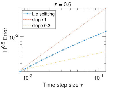
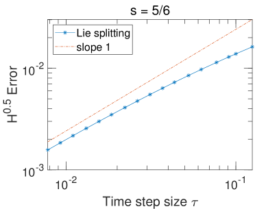
Figure 1. $H^{\frac{1}{2}}$ temporal error of the Lie splitting scheme for the two-dimensional NKG with rough initial data $z_{0}+\langle\nabla\rangle^{-1}z_{1}\in H^{s}$. Left: $s=0.6$;  right: $s=5/6$.

In Figure 1, we performed numerical experiments for the Lie splitting scheme (2.5). Here we normalized the initial data $\|z_{0}+\langle\nabla\rangle^{-1}z_{1}\|_{H^{\frac{1}{2}}}=1$, and took Fourier modes $N=(2^{13},2^{13})$. For the reference solution, we used a small time step size $\tau=2^{-12}$. From the figure on the left, we can see that the numerical results are better than we predicted in Theorem 3.1. Nevertheless, we can clearly observe an order reduction. Here, the reason is that the random initial data may give better properties in $L^{p}$ spaces and the finite Fourier series also contain some smoothening effect. From the figure on the right, we can see that the numerical method converges with order $1$, which fits our theorem very well.

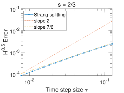
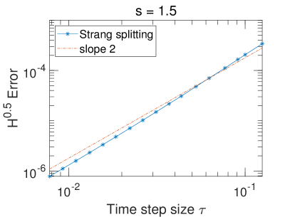
Figure 2. $H^{\frac{1}{2}}$ temporal error of the Strang splitting scheme for the two-dimensional NKG with rough initial data $z_{0}+\langle\nabla\rangle^{-1}z_{1}\in H^{s}$. Left: $s=2/3$;  right: $s=1.5$.

In Figure 2, we performed numerical experiments for the Strang splitting scheme (2.6). Here we again normalized the initial data $\|z_{0}+\langle\nabla\rangle^{-1}z_{1}\|_{H^{\frac{1}{2}}}=1$, and took Fourier modes $N=(2^{13},2^{13})$. For the reference solution, we used a small time step size $\tau=2^{-12}$. From the figure on the left, we can see that the error converges quite well with order $s+\frac{1}{2}$, which coincides with the order we proved for larger $s$ in Theorem 3.1, but is different from what we predicted in Remark 3.5. We observed that the convergence results are better in higher dimensions than in lower dimensions, and we found irregular convergence behavior in the one-dimensional case (see Figure 3). From the figure on the right, we can see that the numerical method converges with order $2$, which fits our theorem very well.

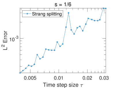
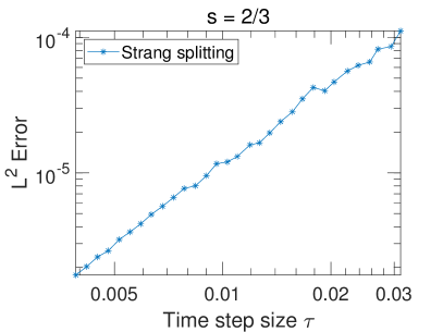
Figure 3. $L^{2}$ temporal error of the Strang splitting scheme for the one-dimensional NKG with rough initial data $z_{0}+\langle\nabla\rangle^{-1}z_{1}\in H^{s}$. Left: $s=1/6$;   right: $s=2/3$.

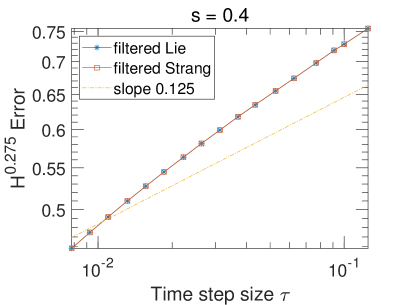
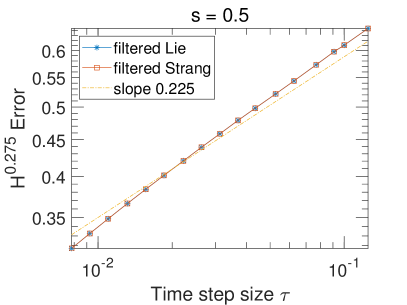
Figure 4. $H^{\frac{11}{40}}$ temporal error of the filtered Lie and Strang splitting schemes for the two-dimensional NKG with very rough initial data $z_{0}+\langle\nabla\rangle^{-1}z_{1}\in H^{s}$. Left: $s=0.4$;  right: $s=0.5$.

In Figure 3, we performed numerical experiments for the Strang splitting scheme (2.6). Here we normalized the initial data as $\|z_{0}+\langle\nabla\rangle^{-1}z_{1}\|_{L^{2}}=1$, and took Fourier modes $N=2^{14}$. For the reference solution, we used a small time step size $\tau=2^{-13}$. From the figure on the left, we can see that the convergence behavior for the borderline case $s=\frac{1}{6}$ is very irregular. However, with the gain of regularity of the initial data, we can see that the convergence behavior becomes regular again. For instance, when $s=\frac{2}{3}>\frac{1}{2}$, as we can see from the figure on the right, the convergence behavior is regular, and the convergence order is almost $2$.

In Figure 4, we performed numerical experiments for the filtered Lie (4.4) and the filtered Strang splitting scheme (4.5). The initial data is normalized as $\|z_{0}+\langle\nabla\rangle^{-1}z_{1}\|_{H^{\frac{11}{40}}}=1$, and we took Fourier modes $N=(2^{13},2^{13})$. For the reference solution, we used a small time step size $\tau=2^{-12}$. From the figure, we can see that the convergence behaviors of the two methods are almost the same. In particular, the Strang splitting does not perform better than Lie. Moreover, the convergence order of the right figure (i.e., when $s=0.5$) is almost $0.225$, which fits Theorem 4.1 very well. However, the figure on the left (i.e., $s=0.4$) shows that the convergence order is a little bit better than predicted by our theorem, the possible reason here is that the reference solution is not accurate enough since the method converges very slow [19, 20].

Funding

This work is supported by NSFC 42450275, 12271413, and the Natural Science Foundation of Hubei Province No. 2019CFA007.

References

- [1] S. Adjerid, H. Temimi, A discontinuous Galerkin method for the wave equation, Comput. Methods Appl. Mech. Engrg. 200, 837–849 (2011).
- [2] W. Bao, Y. Feng, C. Su, Uniform error bounds of a time-splitting spectral method for the long-time dynamics of the nonlinear Klein–Gordon equation with weak nonlinearity, Math. Comp. 91, 811–842 (2022).
- [3] W. Bao, X. Zhao, Comparison of numerical methods for the nonlinear Klein–Gordon equation in the nonrelativistic limit regime, J. Comput. Phys. 398, 108886 (2019).
- [4] D. D. Baǐnov, E. Minchev, Nonexistence of global solutions of the initial-boundary value problem for the nonlinear Klein–Gordon equation, J. Math. Phys. 36, 756–762 (1995).
- [5] L. Berge, B. Bidegaray, T. Colin, A perturbative analysis of the time-envelope approximation in the strong Langmuir turbulence, Phys. D 95 351–379 (1996).
- [6] J. Bourgain, Global Solutions of Nonlinear Schrödinger Equations, American Mathematical Society Colloquium Publications, 46, American Mathematical Society, Providence, RI, 1999.
- [7] J. Bourgain, D. Li, On an endpoint Kato-Ponce inequality, Diff. Int. Eq. 27, 1037–1072 (2014).
- [8] S. Buchholz, B. Dörich, M. Hochbruck, On averaged exponential integrators for semilinear wave equations with solutions of low-regularity, SN Part. Diff. Equ. Appl., 2, 23 (2021).
- [9] M. Christ, J. Colliander, T. Tao, Ill-posedness for nonlinear Schrödinger and wave equations, preprint, arXiv:math/0311048 (2003).
- [10] J. Colliander, M. Keel, G. Staffilani, H. Takaoka, T. Tao, webpage, https://www.math.ucla.edu/˜tao/Dispersive/.
- [11] A. S. Davydov, Quantum Mechanics, 2nd edn., Pergamon, Oxford, 1976.
- [12] D. B. Duncan, Symplectic finite difference approximations of the nonlinear Klein–Gordon equation, SIAM J. Numer. Anal. 34 1742–-1760 (1997).
- [13] X. Dong, Z. Xu, X. Zhao, On time-splitting pseudospectral discretization for nonlinear Klein–Gordon equation in nonrelativistic limit regime, Commun. Comput. Phys. 16 440–466 (2014).
- [14] Y. Gao, L. Mei, R. Li, Galerkin finite element methods for the generalized Klein–Gordon–Zakharov equations, Comput. Math. Appl. 74 2466–2484 (2017).
- [15] J. Ginibre, G. Velo, The global Cauchy problem for the nonlinear Klein–Gordon equation, Math. Z. 189 487–505 (1985).
- [16] J. Ginibre, G. Velo, The global Cauchy problem for the nonlinear Klein–Gordon equation. II, Ann. Inst. H. Poincaré Anal. Non Linéaire 6 15–35 (1989).
- [17] K. Huang, A Superfluid Universe, World Scientific, Hackensack, NJ, 2016.
- [18] E. Hairer, C. Lubich, G. Wanner, Geometric Numerical Integration, Springer-Verlag, 2002.
- [19] L. Ji, A. Ostermann, F. Rousset, K. Schratz, Low regularity full error estimates for the cubic nonlinear Schrödinger equation, SIAM J. Numer. Anal. 62 2071–2086 (2024).
- [20] L. Ji, A. Ostermann, F. Rousset, K. Schratz, Low regularity error estimates for the time integration of 2D NLS, IMA J. Numer. Anal. doi:10.1093/imanum/drae054 (2024).
- [21] L. Ji, H. Li, A. Ostermann, C. Su, Filtered Lie-Trotter splitting for the “good” Boussinesq equation: low regularity error estimates, Math. Comp. doi: 10.1090/mcom/4023 (2024).
- [22] T. Kato, G. Ponce, Commutator estimates and the Euler and Navier-Stokes equations, Commun. Pure Appl. Math. 41 891–907 (1988).
- [23] B. Li, K. Schratz, F. Zivcovich, A second-order low-regularity correction of Lie splitting for the semilinear Klein–Gordon equation, ESAIM: Math. Model. Numer. Anal. 57 899–919 (2023).
- [24] X. Li, B. Guo, A Legendre spectral method for solving the nonlinear Klein–Gordon equation, J. Comput. Math. 15 105–126 (1997).
- [25] C. Liu, A. Iserles, X. Wu, Symmetric and arbitrarily high-order Birkhoff-Hermite time integrators and their long-time behaviour for solving nonlinear Klein–Gordon equations, J. Comp. Phys. 356 1–30 (2018).
- [26] H. Lindblad, C. Sogge, On existence and scattering with minimal regularity for semilinear wave equations, J. Func. Anal. 130 357–426 (1995).
- [27] N.J. Mauser, Y. Zhang, X. Zhao, On the rotating nonlinear Klein–Gordon equation: nonrelativistic limit and numerical methods, Multiscale Model. Simul. 18 999–1024 (2020).
- [28] A. Ostermann, K. Schratz, Low regularity exponential-type integrators for semilinear Schrödinger equations, Found. Comput. Math. 18 731–755 (2018).
- [29] A. Ostermann, F. Rousset, K. Schratz, Fourier integrator for periodic NLS: low regularity estimates via discrete Bourgain spaces, J. Eur. Math. Soc. 25 3913–3952 (2023).
- [30] A. Ostermann, F. Rousset, K. Schratz, Error estimates at low regularity of splitting schemes for NLS, Math. Comp. 91 169–182 (2022).
- [31] F. Rousset, K. Schratz, Convergence error estimates at low regularity for time discretizations of KdV, Pure Appl. Anal. 4 127–152 (2022).
- [32] T. Tao, Nonlinear dispersive equations: local and global analysis, Amer. Math. Soc. Providence RI, 2006.
- [33] Y. Wang, X. Zhao, A symmetric low-regularity integrator for nonlinear Klein–Gordon equation, Math. Comp. 91 2215–2245 (2022).