Distributionally Robust Active Learning
for Gaussian Process Regression

Abstract

Gaussian process regression (GPR) or kernel ridge regression is a widely used and powerful tool for nonlinear prediction. Therefore, active learning (AL) for GPR, which actively collects data labels to achieve an accurate prediction with fewer data labels, is an important problem. However, existing AL methods do not theoretically guarantee prediction accuracy for target distribution. Furthermore, as discussed in the distributionally robust learning literature, specifying the target distribution is often difficult. Thus, this paper proposes two AL methods that effectively reduce the worst-case expected error for GPR, which is the worst-case expectation in target distribution candidates. We show an upper bound of the worst-case expected squared error, which suggests that the error will be arbitrarily small by a finite number of data labels under mild conditions. Finally, we demonstrate the effectiveness of the proposed methods through synthetic and real-world datasets.

1 Introduction

Active learning (AL) (Settles, 2009) is a framework for achieving high prediction performance with fewer data when labeling new data is expensive. For this purpose, AL algorithms actively acquire the label of data that improves the prediction performance of some statistical model based on acquisition functions (AFs). Many types of AFs have been proposed, such as uncertainty sampling (US), random sampling (RS), variance reduction, and information gain, as summarized in Settles (2009).

Gaussian process regression (GPR) model (Rasmussen and Williams, 2005) is often used as a base statistical model for AL algorithms due to its flexible prediction capability (Seo et al., 2000; Yu et al., 2006; Guestrin et al., 2005; Krause et al., 2008b; Hoang et al., 2014). Standard AL methods for the GPR are based on information gaion (Guestrin et al., 2005; Krause et al., 2008b; Kirsch et al., 2021; Kirsch and Gal, 2022; Bickford Smith et al., 2023). Most information gain-based approaches are heuristics without theoretical guarantees. A notable exception is the work by Guestrin et al. (2005); Krause et al. (2008b), which shows the US for the GPR model is optimal to maximize the information gain from the obtained data labels regarding GP prior. Furthermore, from the analysis of kernelized bandits (e.g., Srinivas et al., 2010; Salgia et al., 2024), we can see that the US and RS guarantee the convergence of the maximum of posterior variance (See Proposition 2.3 for details). Another commonly used AF is variance reduction (Seo et al., 2000; Yu et al., 2006; Shoham and Avron, 2023), which can be computed efficiently in the GPR. However, these AFs do not incorporate the importance of the unlabelled dataset, that is, the prior information regarding the target distribution. In addition, to our knowledge, except for the worst-case analysis in Proposition 2.3, there are no theoretical guarantees for the target prediction error.

Several studies have tackled the development of the target distribution-aware AL (Kirsch et al., 2021; Kirsch and Gal, 2022; Bickford Smith et al., 2023). In particular, as an extension of the distributionally robust learning (Chen et al., 2020), Frogner et al. (2021) proposed distributionally robust AL (DRAL), which aims to minimize the worst-case error in the set of target distributions to obtain a robust model. However, since these studies employed the heuristic AL methods based on, e.g., information gain and expected model change (Settles, 2009), the theoretical guarantee has not been shown.

This paper develops a DRAL framework for the GPR model. We aim to minimize the worst-case expected error, where the worst-case scenario and the expectation are taken regarding the target distribution candidates and chosen target distributions, respectively. Note that our formulation is a generalization of target distribution-aware AL since it includes the case in which the unique target distribution can be specified. We perform the theoretical analysis under two conditions called Bayesian and frequentist assumptions (Srinivas et al., 2010), in which we leverage several useful lemmas in kernelized bandit literature (Srinivas et al., 2010; Vakili et al., 2021a, b; Kusakawa et al., 2022).

Our contributions are summarized as follows:

1. We show several properties of the worst-case squared error for the GPR model, which suggests that the error can be bounded from above using the posterior variance even if the input domain is continuous. Along the way to proving the error properties, we show the Lipschitz constant of the posterior mean of GPs in Lemmas 2.9 and 3.3, which may be of independent interest.

2. We propose two DRAL methods for the GPR model, inspired by the RS and the greedy algorithm. Our proposed methods are designed to guarantee the convergence of the (expected) posterior variance.

3. We show the probabilistic upper bounds of the error incurred by the proposed algorithm, which suggests that under mild conditions, the error can be arbitrarily small by a finite number of data labels.

Finally, we demonstrate the effectiveness of the proposed methods via synthetic and real-world regression problems.

2 Background

This section provides the known properties of the GPR.

2.1 GPR model

The GPR model (Rasmussen and Williams, 2005) is a kernel-based regression model. Let us consider that we have already obtained the training dataset of input-output pair ${\cal D}_{t}=\{(\boldsymbol{x}_{i},y_{\boldsymbol{x}_{i}})\}_{i=1}^{t}$, where $\forall i,\boldsymbol{x}_{i}\in{\cal X}\subset\mathbb{R}^{d}$, $y_{\boldsymbol{x}_{i}}\in\mathbb{R}$, and $d$ is an input dimension. The GPR model assumes that, without loss of generality, $f$ follows zero-mean GP, that is, $f\sim{\cal G}{\cal P}(0,k)$, where $k:{\cal X}\times{\cal X}\mapsto\mathbb{R}$ is a predefined positive semidefinite kernel function. In addition, the $i$-th observation $y_{\boldsymbol{x}_{i}}$ is assumed to be contaminated by i.i.d. Gaussian noise $\epsilon_{i}\sim{\cal N}(0,\sigma^{2})$ as $y_{\boldsymbol{x}_{i}}=f(\boldsymbol{x}_{i})+\epsilon_{i}$. Then, the posterior distribution of $f$ becomes again a GP, whose mean and variance are analytically derived as follows:

$$\begin{split}\mu_{t}(\boldsymbol{x})&=\boldsymbol{k}_{t}(\boldsymbol{x})^{\top}\bigl{(}\boldsymbol{K}+\sigma^{2}\boldsymbol{I}_{t}\bigr{)}^{-1}\boldsymbol{y}_{t},\\ \sigma_{t}^{2}(\boldsymbol{x})&=k(\boldsymbol{x},\boldsymbol{x})-\boldsymbol{k}_{t}(\boldsymbol{x})^{\top}\bigl{(}\boldsymbol{K}+\sigma^{2}\boldsymbol{I}_{t}\bigr{)}^{-1}\boldsymbol{k}_{t}(\boldsymbol{x}),\end{split}$$ (1)

where $\boldsymbol{k}_{t}(\boldsymbol{x})\coloneqq\bigl{(}k(\boldsymbol{x},\boldsymbol{x}_{1}),\dots,k(\boldsymbol{x},\boldsymbol{x}_{t})\bigr{)}^{\top}\in\mathbb{R}^{t}$, $\boldsymbol{K}\in\mathbb{R}^{t\times t}$ is the kernel matrix whose $(i,j)$-element is $k(\boldsymbol{x}_{i},\boldsymbol{x}_{j})$, $\boldsymbol{I}_{t}\in\mathbb{R}^{t\times t}$ is the identity matrix, and $\boldsymbol{y}_{t}\coloneqq(y_{\boldsymbol{x}_{1}},\dots,y_{\boldsymbol{x}_{t}})^{\top}\in\mathbb{R}^{t}$. Finally, for later use, let the posterior variance at $\boldsymbol{x}^{*}$ when $\boldsymbol{x}_{t}=\boldsymbol{x}$ be $\sigma_{t}^{2}(\boldsymbol{x}^{*}\mid\boldsymbol{x})\coloneqq\sigma_{t}^{2}(\boldsymbol{x}^{*}\mid\boldsymbol{x}_{t}=\boldsymbol{x})$. Note that the posterior variance calculation does not require $\boldsymbol{y}_{t}$. Furthermore, it is known that $\mu_{t}(\boldsymbol{x})$ is equivalent to the kernel ridge regression estimator with regularization parameter $\lambda=\sigma^{2}$ (Kanagawa et al., 2018).

Maximum Information Gain (MIG):

Further, we define MIG (Srinivas et al., 2010; Vakili et al., 2021b):

Definition 2.1 (Maximum information gain).

Let $f\sim{\cal G}{\cal P}(0,k)$ over ${\cal X}\subset[0,r]^{d}$. Let $A=\{\boldsymbol{a}_{i}\}_{i=1}^{T}\subset{\cal X}$. Let $\boldsymbol{f}_{A}=\bigl{(}f(\boldsymbol{a}_{i})\bigr{)}_{i=1}^{T}$, $\boldsymbol{\epsilon}_{A}=\bigl{(}\epsilon_{i}\bigr{)}_{i=1}^{T}$, where $\forall i,\epsilon_{i}\sim{\cal N}(0,\sigma^{2})$, and $\boldsymbol{y}_{A}=\boldsymbol{f}_{A}+\boldsymbol{\epsilon}_{A}\in\mathbb{R}^{T}$. Then, MIG $\gamma_{T}$ is defined as follows:

$$\gamma_{T}\coloneqq\max_{A\subset{\cal X};|A|=T}I(\boldsymbol{y}_{A};\boldsymbol{f}_{A}),$$

where $I$ is the Shannon mutual information.

It is known that MIG is sublinear for commonly used kernel functions, for example, $\gamma_{T}={\cal O}\bigl{(}d\log T\bigr{)}$ for linear kernels, $\gamma_{T}={\cal O}\bigl{(}(\log T)^{d+1}\bigr{)}$ for squared exponential (SE) kernels $k_{\rm SE}(\boldsymbol{x},\boldsymbol{x}^{\prime})=\exp\left(-\|\boldsymbol{x}-\boldsymbol{x}^{\prime}\|_{2}^{2}/(2\ell^{2})\right)$, and $\gamma_{T}={\cal O}\bigl{(}T^{\frac{d}{2\nu+d}}(\log T)^{\frac{2\nu}{2\nu+d}}\bigr{)}$ for Matérn-$\nu$ kernels $k_{\rm Mat}=\frac{2^{1-\nu}}{\Gamma(\nu)}\left(\frac{\sqrt{2\nu}\|\boldsymbol{x}-\boldsymbol{x}^{\prime}\|_{2}}{\ell}\right)^{\nu}J_{\nu}\left(\frac{\sqrt{2\nu}\|\boldsymbol{x}-\boldsymbol{x}^{\prime}\|_{2}}{\ell}\right)$, where $\ell,\nu>0$ are the lengthscale and smoothness parameter, respectively, and $\Gamma(\cdot)$ and $J_{\nu}$ are Gamma and modified Bessel functions, respectively (Srinivas et al., 2010; Vakili et al., 2021b).

Lipschitz Consatant of $\sigma_{t}(\boldsymbol{x})$:

We will use the following useful result from Theorem E.4 in Kusakawa et al. (2022):

Lemma 2.2 (Lipschitz constant for posterior standard deviation).

Let $k(\boldsymbol{x},\boldsymbol{x}^{\prime}):\mathbb{R}^{d}\times\mathbb{R}^{d}\to\mathbb{R}$ be linear, SE, or Matérn-$\nu$ kernel and $k(\boldsymbol{x},\boldsymbol{x})\leq 1$. Moreover, assume that a noise variance $\sigma^{2}$ is positive. Then, for any $t\geq 1$ and ${\cal D}_{t}$, the posterior standard deviation $\sigma_{t}(\boldsymbol{x})$ satisfies that

$$\forall\boldsymbol{x},\boldsymbol{x}^{\prime}\in\mathbb{R}^{d},\ |\sigma_{t}(\boldsymbol{x})-\sigma_{t}(\boldsymbol{x}^{\prime})|\leq L_{\sigma}\|\boldsymbol{x}-\boldsymbol{x}^{\prime}\|_{1},$$

where $L_{\sigma}$ is a positive constant given by

$$L_{\sigma}=\left\{\begin{array}[]{ll}1&\text{if $k(\boldsymbol{x},\boldsymbol{x}^{\prime})$ is the linear kernel},\\ \frac{\sqrt{2}}{\ell}&\text{if $k(\boldsymbol{x},\boldsymbol{x}^{\prime})$ is the SE kernel},\\ \frac{\sqrt{2}}{\ell}\sqrt{\frac{\nu}{\nu-1}}&\text{if $k(\boldsymbol{x},\boldsymbol{x}^{\prime})$ is the Mat\'{e}rn kernel},\end{array}\right.$$

where $\nu>1$.

2.2 Uncerrainty Sampling and Random Sampling

For the GPR model, the US selects the most uncertain input as $t$-th input:

$$\boldsymbol{x}_{t}=\operatorname*{arg\,max}_{\boldsymbol{x}\in{\cal X}}\sigma^{2}_{t-1}(\boldsymbol{x}).$$

The RS randomly selects a $t$-th input by a fixed probability distribution $p(\boldsymbol{x})$ over ${\cal X}$:

$$\boldsymbol{x}_{t}\sim p(\boldsymbol{x}).$$

For both algorithms, the upper bound of the maximum variance is known:

Proposition 2.3.

Assume ${\cal X}$ is a compact subset of $\mathbb{R}^{d}$. If we run the US, the following inequality holds:

$$\max_{\boldsymbol{x}\in{\cal X}}\sigma^{2}_{T}(\boldsymbol{x})\leq\frac{C_{1}\gamma_{T}}{T},$$

where $C_{1}=1/\log(1+\sigma^{-2})$. Furthermore, if we run the RS, the following inequality holds with probability at least $1-\delta$, where $\delta\in(0,1)$, under several conditions:

$$\max_{\boldsymbol{x}\in{\cal X}}\sigma^{2}_{T}(\boldsymbol{x})={\cal O}\left(\frac{\sigma^{2}\gamma_{T}}{T}\right).$$

Proof.

For the US, see, e.g., Eq. (16) in Vakili et al. (2021a) and Lemma 5.4 in Srinivas et al. (2010). For the RS, see Theorem 3.1 in Salgia et al. (2024). ∎

When $\gamma_{T}$ is sublinear, the above upper bounds suggest that the maximum variance will be arbitrarily small within the finite time horizons.

2.3 Regularity Assumptions and Predictive Guarantees

Here, we provide the details of Bayesian and frequentist assumptions and predictive guarantees for both assumptions.

2.3.1 Bayesian Assumption

We consider the following assumption:

Assumption 2.4.

The function $f$ is a sample path $f\sim{\cal G}{\cal P}(0,k)$ and the $i$-th observation $y_{\boldsymbol{x}_{i}}$ is contaminated by i.i.d. Gaussian noise $\epsilon_{i}\sim{\cal N}(0,\sigma^{2})$ as $y_{\boldsymbol{x}_{i}}=f(\boldsymbol{x}_{i})+\epsilon_{i}$. In addition, the kernel function is normalized as $k(\boldsymbol{x},\boldsymbol{x}^{\prime})\leq 1$ for all $\boldsymbol{x},\boldsymbol{x}^{\prime}\in{\cal X}$.

Furthermore, for continuous ${\cal X}$, we assume the following smoothness condition:

Assumption 2.5.

Let ${\cal X}\subset[0,r]^{d}$ be a compact set, where $r>0$. Assume that the kernel $k$ satisfies the following condition on the derivatives of a sample path $f$. There exist the constants $a,b>0$ such that,

$$\Pr\left(\sup_{\boldsymbol{x}\in{\cal X}}\left|\frac{\partial f(\boldsymbol{u})}{\partial u_{j}}\Big{|}_{\boldsymbol{u}=\boldsymbol{x}}\right|>L\right)\leq a\exp\left(-\frac{L^{2}}{b^{2}}\right),$$

for all $j\in[d]$.

This assumption holds for stationary and four times differentiable kernels (Theorem 5 of Ghosal and Roy, 2006), such as SE kernel and Matérn-$\nu$ kernels with $\nu>2$ (Section 4 of Srinivas et al., 2010). These assumptions are commonly used (Srinivas et al., 2010; Kandasamy et al., 2018; Paria et al., 2020; Takeno et al., 2023, 2024).

As with Lemma 5.1 in Srinivas et al. (2010), the credible interval can be obtained as follows:

Lemma 2.6.

Suppose that ${\cal X}$ is finite and Assumption 2.4 holds. Pick $\delta\in(0,1)$ and $t\in\mathbb{N}$. Then, for any given ${\cal D}_{t}$,

$$\Pr\left(|f(\boldsymbol{x})-\mu_{t}(\boldsymbol{x})|\leq\beta^{1/2}_{\delta}\sigma_{t}(\boldsymbol{x}),\forall\boldsymbol{x}\in{\cal X}\mid{\cal D}_{t}\right)\geq 1-\delta,$$

where $\beta_{\delta}=2\log(|{\cal X}|/\delta)$.

2.3.2 Frequentist Assumption

We assume that $f$ is an element of the reproducing kernel Hilbert space (RKHS) specified by the kernel $k$ as with Srinivas et al. (2010); Chowdhury and Gopalan (2017); Vakili et al. (2021a, 2022); Li and Scarlett (2022):

Assumption 2.7.

Let $f$ be an element of RKHS ${\cal H}_{k}$ specified by the kernel $k$ used in the GPR model. Furthermore, the RKHS norm of $f$ is bounded as $\|f\|_{{\cal H}_{k}}\leq B<\infty$ for some $B>0$, where $\|\cdot\|_{{\cal H}_{k}}$ denotes the RKHS norm of ${\cal H}_{k}$. In addition, the $i$-th observation $y_{\boldsymbol{x}_{i}}$ is contaminated by independent sub-Gaussian noises $\{\epsilon_{i}\}_{i\in\mathbb{N}}$ as $y_{\boldsymbol{x}_{i}}=f(\boldsymbol{x}_{i})+\epsilon_{i}$. That is, for all $i\in\mathbb{N}$, for all $\eta\in\mathbb{R}$, and for some $R>0$, the moment generating function of $\epsilon_{i}$ satisfies $\mathbb{E}[\exp(\eta\epsilon_{i})]\leq\exp\bigl{(}\frac{\eta^{2}R^{2}}{2}\bigr{)}$. Finally, the kernel function is normalized as $k(\boldsymbol{x},\boldsymbol{x}^{\prime})\leq 1$ for all $\boldsymbol{x},\boldsymbol{x}^{\prime}\in{\cal X}$.

Furthermore, for continuous ${\cal X}$, we assume the following smoothness condition as with Chowdhury and Gopalan (2017); Vakili et al. (2021a, 2022):

Assumption 2.8.

The kernel function $k$ satisfies the following condition on the derivatives. There exists a constant $L_{k}$ such that,

$$\sup_{\boldsymbol{x}\in{\cal X}}\sup_{j\in[d]}\left|\frac{\partial^{2}k(\boldsymbol{u},\boldsymbol{v})}{\partial u_{j}\partial v_{j}}\bigg{|}_{\boldsymbol{u}=\boldsymbol{v}=\boldsymbol{x}}\right|^{1/2}\leq L_{k}.$$

This assumption provides the Lipschitz constant of $f$:

Lemma 2.9 (Lemma 5.1 in De Freitas et al. (2012)).

Suppose that Assumption 2.8 holds. Then, any $g\in{\cal H}_{k}$ is Lipschitz continuous with respect to $\|g\|_{{\cal H}_{k}}L_{k}$.

We rely on the confidence bounds for non-adaptive sampling methods, which is a direct consequence of Theorem 1 in Vakili et al. (2021a) and the union bound:

Lemma 2.10.

Suppose that ${\cal X}$ is finite and Assumption 2.7 holds. Pick $\delta\in(0,1)$ and $t\in\mathbb{N}$. Assume that $(\boldsymbol{x}_{i})_{i\in[t]}$ is independent of $(\epsilon_{i})_{i\in[t]}$. Then, the following holds:

$$\Pr\left(|f(\boldsymbol{x})-\mu_{t}(\boldsymbol{x})|\leq\beta^{1/2}_{\delta}\sigma_{t}(\boldsymbol{x}),\forall\boldsymbol{x}\in{\cal X}\right)\geq 1-\delta,$$

where $\beta_{\delta}=\left(B+\frac{R}{\sigma}\sqrt{2\log(\frac{2|{\cal X}|}{\delta})}\right)^{2}$.

3 Problem Statements and Its Property

This section provides our problem setup and its properties.

3.1 Problem Statement

We aim to minimize the worst-case expected errors regarding the GP prediction $\mu_{T}(\boldsymbol{x})$ after $T$-th function evaluations:

$$E_{T} \coloneqq\max_{p\in{\cal P}}\mathbb{E}_{p(\boldsymbol{x}^{*})}\left[(f(\boldsymbol{x}^{*})-\mu_{T}(\boldsymbol{x}^{*}))^{2}\right],$$ (2)

where ${\cal P}$ is a set of target distributions over the input space ${\cal X}$ called ambiguity set (Chen et al., 2020). We assume that $\max_{p\in{\cal P}}\mathbb{E}_{p(\boldsymbol{x}^{*})}\left[g(\boldsymbol{x}^{*})\right]$ exists for any continuous function $g:{\cal X}\rightarrow\mathbb{R}$. This paper concentrates on the setting where the training input space from which we can obtain labels includes the test input space.

Our problem setup can be seen as the generalization of the target distribution-aware AL and the AL for the worst-case error $\max_{\boldsymbol{x}\in{\cal X}}(f(\boldsymbol{x})-\mu_{T}(\boldsymbol{x}))^{2}$. This is because our problem is equivalent to the target distribution-aware AL if we set $|{\cal P}|=1$ and to the worst-case error minimization if ${\cal P}$ includes $\{p\in{\cal P}_{{\cal X}}\mid\exists\boldsymbol{x}\in{\cal X},p(\boldsymbol{x})=1\}$, where ${\cal P}_{\rm{\cal X}}$ is the set of the distributions over ${\cal X}$.

3.2 High Probability Bound of Error

If the input space ${\cal X}$ is finite, we can obtain the upper bound of Eq. (2) as the direct consequence of Lemmas 2.6 and 2.10:

Lemma 3.1.

Fix $\delta\in(0,1)$ and $T\in\mathbb{N}$. Suppose that Assumption 2.4 holds and $\beta_{\delta}$ is set as in Lemma 2.6, or Assumption 2.7 holds and $\beta_{\delta}$ is set as in Lemma 2.10. Then, the following holds with probability at least $1-\delta$:

$$E_{T} \leq\beta_{\delta}\max_{p\in{\cal P}}\mathbb{E}_{p(\boldsymbol{x}^{*})}\left[\sigma^{2}_{T}(\boldsymbol{x}^{*})\right].$$

For continuous ${\cal X}$, the confidence parameter $\beta_{\delta}\propto\log|{\cal X}|$ diverges if we apply Lemmas 2.6 and 2.10 directly. Therefore, in this case, the Lipschitz property is often leveraged (Chowdhury and Gopalan, 2017; Vakili et al., 2021a). The Lipschitz constant of $f$ can be directly derived from the Assumption 2.5, or Assumption 2.8 and Lemma 2.9 (Srinivas et al., 2010; De Freitas et al., 2012).

Furthermore, we need the Lipschitz constant of $\mu_{T}$. In the frequentist setting, the Lipschitz constant for $\mu_{T}$ can be derived as ${\cal O}(L_{k}\sqrt{t\log t})$ by Lemma 4 in Vakili et al. (2021a) and Lemma 2.9. To obtain a slightly tighter upper bound, we show the following lemma:

Lemma 3.2.

Fix $\delta\in(0,1)$ and $t\in[T]$. Suppose that Assumptions 2.7 and  2.8 hold. Then, $\mu_{t}(\cdot)$ is Lipschitz continuous with the Lipschitz constant,

$$L_{k}\left(B+\frac{R}{\sigma}\sqrt{2\gamma_{t}+2\log\left(\frac{d}{\delta}\right)}\right)$$

with probability at least $1-\delta$.

We show the proof in Appendix A.1. Since the MIG $\gamma_{T}$ is sublinear for the kernels on which we mainly focus, the upper bound ${\cal O}(L_{k}\sqrt{\gamma_{t}})$ is tighter than ${\cal O}(L_{k}\sqrt{t\log t})$.

In the Bayesian setting, the upper bound of the Lipschitz constant for $\mu_{T}$ has not been shown to our knowledge. Therefore, we show the following lemma:

Lemma 3.3.

Fix $\delta\in(0,1)$ and $t\in[T]$. Suppose that Assumptions 2.4 and 2.5 hold and the kernel has mixed partial derivative $\frac{\partial^{2}k(\boldsymbol{x},\boldsymbol{z})}{\partial x_{j}\partial z_{j}}$ for all $j\in[d]$. Set $a$ and $b$ as in Lemma 2.5. Assume that $(\boldsymbol{x}_{i})_{i\in[t]}$ is independent of $(\epsilon_{i})_{i\in[t]}$ and $f$. Then, $\mu_{t}$ and $r_{t}(\boldsymbol{x})\coloneqq f(\boldsymbol{x})-\mu_{t}(\boldsymbol{x})$ satisfies the following:

$$\Pr\left(\sup_{\boldsymbol{x}\in{\cal X}}\left|\frac{\partial\mu_{t}(\boldsymbol{u})}{\partial u_{j}}\Big{|}_{\boldsymbol{u}=\boldsymbol{x}}\right|>L\right)\leq 2a\exp\left(-\frac{L^{2}}{b^{2}}\right),$$

$$\Pr\left(\sup_{\boldsymbol{x}\in{\cal X}}\left|\frac{\partial r_{t}(\boldsymbol{u})}{\partial u_{j}}\Big{|}_{\boldsymbol{u}=\boldsymbol{x}}\right|>L\right)\leq 2a\exp\left(-\frac{L^{2}}{b^{2}}\right),$$

for all $j\in[d]$.

See Appendix A.2 for the proof, in which we leverage Slepian’s inequality (Proposition A.2.6 in van der Vaart and Wellner, 1996) and the fact that the derivative of the sample path follows GP jointly when the kernel is differentiable.

By leveraging the above results, even if ${\cal X}$ is continuous, we can obtain the following upper bound of Eq. (2):

Lemma 3.4.

Suppose that Assumptions 2.7 and  2.8 hold. Fix $\delta\in(0,1)$ and $T\in\mathbb{N}$. Then, the following holds with probability at least $1-\delta$:

$$E_{T} \leq 2\beta_{\delta,T}\max_{p\in{\cal P}}\mathbb{E}_{p(\boldsymbol{x}^{*})}\left[\sigma_{T}^{2}(\boldsymbol{x}^{*})\right]+{\cal O}\left(\frac{\max\{\gamma_{T},\log(\frac{T}{\delta})\}}{T^{2}}\right).$$

where $\beta_{\delta,T}=\left(B+\frac{R}{\sigma}\sqrt{2d\log\left(Tdr+1\right)+2\log\left(\frac{4}{\delta}\right)}\right)^{2}$.

Lemma 3.5.

Suppose that Assumptions 2.4 and 2.5 hold. Fix $\delta\in(0,1)$ and $T\in\mathbb{N}$. Then, the following holds with probability at least $1-\delta$:

$$E_{T} \leq 2\beta_{\delta,T}\max_{p\in{\cal P}}\mathbb{E}_{p(\boldsymbol{x}^{*})}\left[\sigma_{T}^{2}(\boldsymbol{x}^{*})\right]+{\cal O}\left(\frac{\log(\frac{T}{\delta})}{T^{2}}\right),$$

where $\beta_{\delta,T}=2d\log(Tdr+1)+2\log(2/\delta)$.

See Appendices A.3 and  A.4 for the proof.

Consequently, we can minimize Eq. (2) by minimizing $\max_{p\in{\cal P}}\mathbb{E}_{p(\boldsymbol{x}^{*})}\left[\sigma^{2}_{T}(\boldsymbol{x}^{*})\right]$. In this perspective, the US and RS are theoretically guaranteed because of $\max_{p\in{\cal P}}\mathbb{E}_{p(\boldsymbol{x}^{*})}\left[\sigma^{2}_{T}(\boldsymbol{x}^{*})\right]\leq\max_{\boldsymbol{x}\in{\cal X}}\sigma^{2}_{T}(\boldsymbol{x})$ and Proposition 2.3. However, the US and RS do not incorporate the information of ${\cal P}$. Therefore, the practical effectiveness of the US and RS is limited.

3.3 Other Performance Mesuares

Although we mainly discuss the squared error, other measures can also be bounded from above:

Lemma 3.6.

The worst-case expected absolute error for any $T\in\mathbb{N}$ is bounded from above as follows:

$$\max_{p\in{\cal P}}\mathbb{E}_{p(\boldsymbol{x}^{*})}\left[|f(\boldsymbol{x}^{*})-\mu_{T}(\boldsymbol{x}^{*})|\right]\leq\sqrt{E_{T}},$$

where $E_{T}$ is defined as in Eq. (2).

Lemma 3.7.

The worst-case expectation of entropy for any $T\in\mathbb{N}$ is bounded from above as follows:

$$\max_{p\in{\cal P}}\mathbb{E}_{p(\boldsymbol{x}^{*})}\left[H\left[f(\boldsymbol{x}^{*})\mid{\cal D}_{T}\right]\right] \leq\frac{1}{2}\log\left(2\pi e\tilde{E}_{T}\right),$$

where $\tilde{E}_{T}=\max_{p\in{\cal P}}\mathbb{E}_{p(\boldsymbol{x}^{*})}\left[\sigma^{2}_{T}(\boldsymbol{x}^{*})\right]$ and $H[f(\boldsymbol{x})\mid{\cal D}_{T}]=\log\left(\sqrt{2\pi e}\sigma_{T}(\boldsymbol{x})\right)$ is Shannon entropy.

See Appendices A.5 and A.6 for the proof. Therefore, minimizing $\max_{p\in{\cal P}}\mathbb{E}_{p(\boldsymbol{x}^{*})}\left[\sigma^{2}_{T}(\boldsymbol{x}^{*})\right]$ also provides the convergence of the absolute error and the entropy.

4 Proposed Methods and Analysis

We aim to design algorithms that enjoy both a similar convergence guarantee as the US and RS and practical effectiveness incorporating the information of ${\cal P}$. In particular, we consider two algorithms inspired by the greedy algorithm and the RS and show theoretical guarantees. Algorithm 1 shows the pseudo-code of proposed algorithms.

Algorithm 1 Proposed DRAL methods

1:Domain ${\cal X}$, GP prior $\mu$ and $k$, ambiguity set ${\cal P}$

2:${\cal D}_{0}\leftarrow\emptyset$

3:for $t=1,\dots,T$ do

4:  Update $\sigma_{t-1}^{2}(\cdot)$ according to Eq. (1)

5:  Compute $\boldsymbol{x}_{t}$ according to Eq. (3) or Eq. (4)

6:end for

7:Observe $y_{1},\dots,y_{T}$

8:Update $\mu_{T}(\cdot)$ and $\sigma_{T}^{2}(\cdot)$ according to Eq. (1)

9:return $\mu_{T}(\cdot)$ and $\sigma_{T}^{2}(\cdot)$

4.1 Algorithms

First, we consider the RS-based algorithm. The algorithm is straightforward as follows:

$$\boldsymbol{x}_{t}\sim p_{t}(\boldsymbol{x}),$$ (3)

where $p_{t}(\boldsymbol{x})=\operatorname*{arg\,max}_{p\in{\cal P}}\mathbb{E}_{p(\boldsymbol{x}^{*})}[\sigma_{t-1}^{2}(\boldsymbol{x}^{*})]$ and we assume that we can generate the sample from $p_{t}$. By using the worst-case distribution $p_{t}$ for each iteration, this algorithm incorporates the information of ${\cal P}$.

Second, we consider the greedy algorithm since its practical efficiency has often been reported (e.g., Bian et al., 2017). However, in our setup, the greedy algorithm should be

$$\operatorname*{arg\,min}_{\boldsymbol{x}\in{\cal X}}\max_{p\in{\cal P}}\mathbb{E}_{p(\boldsymbol{x}^{*})}[\sigma_{t}^{2}(\boldsymbol{x}^{*}\mid\boldsymbol{x})],$$

which requires huge computational time in general due to min-max optimization. Thus, we consider an approximately greedy algorithm as follows:

$$\operatorname*{arg\,min}_{\boldsymbol{x}\in{\cal X}}\mathbb{E}_{p_{t}(\boldsymbol{x}^{*})}[\sigma_{t}^{2}(\boldsymbol{x}^{*}\mid\boldsymbol{x})],$$

where $p_{t}(\boldsymbol{x})=\operatorname*{arg\,max}_{p\in{\cal P}}\mathbb{E}_{p(\boldsymbol{x}^{*})}[\sigma_{t-1}^{2}(\boldsymbol{x}^{*})]$ is the worst-case distribution defined by $(\boldsymbol{x}_{i})_{i\in[t-1]}$. On the other hand, the theoretical guarantee for this algorithm is challenging for us. Hence, inspired by the fact that the US has a theoretical guarantee, we set the constraint so that the chosen input is uncertain than $\mathbb{E}_{p_{t}(\boldsymbol{x}^{*})}[\sigma_{t-1}^{2}(\boldsymbol{x}^{*})]$:

$$\boldsymbol{x}_{t}=\operatorname*{arg\,min}_{\boldsymbol{x}\in{\cal X}_{t}}\mathbb{E}_{p_{t}(\boldsymbol{x}^{*})}[\sigma_{t}^{2}(\boldsymbol{x}^{*}\mid\boldsymbol{x})],$$ (4)

where ${\cal X}_{t}\coloneqq\{\boldsymbol{x}\in{\cal X}\mid\sigma^{2}_{t-1}(\boldsymbol{x})\geq\mathbb{E}_{p_{t}(\boldsymbol{x}^{*})}[\sigma_{t-1}^{2}(\boldsymbol{x}^{*})]\}$. Note that $|{\cal X}_{t}|\geq 1$ holds due to the definition.

4.2 Analysis

Here, we show the error convergence by Eqs. (3) and (4):

Theorem 4.1.

Fix $\delta\in(0,1)$. Assume that ${\cal X}\subset\mathbb{R}^{d}$ is a compact subset. If we run Algorithm 1 with Eq. (3), the following holds with probability at least $1-\delta$:

$$\max_{p\in{\cal P}}\mathbb{E}_{p(\boldsymbol{x}^{*})}[\sigma_{T}^{2}(\boldsymbol{x}^{*})] \leq\frac{2C_{1}\gamma_{T}}{T}+{\cal O}\left(\frac{\log(1/\delta)}{T}\right),$$

where $C_{1}=1/\log(1+\sigma^{-2})$.

Theorem 4.2.

Assume that ${\cal X}\subset\mathbb{R}^{d}$ is a compact subset. If we run Algorithm 1 with Eq. (4), the following holds:

$$\max_{p\in{\cal P}}\mathbb{E}_{p(\boldsymbol{x}^{*})}[\sigma_{T}^{2}(\boldsymbol{x}^{*})] \leq\frac{C_{1}\gamma_{T}}{T},$$

where $C_{1}=1/\log(1+\sigma^{-2})$.

See Appendix B for the proof, in which Lemma 3 in Kirschner and Krause (2018) is used to show Theorem 4.1.

Consequently, our proposed methods achieve almost the same convergence as those of the US and RS shown in Proposition 2.3. Furthermore, by combining Lemmas 3.1, 3.4, and 3.5, we can see that the upper bound of $E_{T}$:

Corollary 4.3.

Fix $\delta\in(0,1)$ and $T\in\mathbb{N}$. Then, if we run Algorithm 1, the following hold with probability at least $1-\delta$:

1. When Assumption 2.4 or Assumptions 2.7 holds,

   $$E_{T}={\cal O}\left(\frac{\log(|{\cal X}|/\delta)\gamma_{T}}{T}\right);$$

2. When Assumptions 2.4 and 2.5 or Assumptions 2.7 and 2.8 hold,

   $$E_{T}={\cal O}\left(\frac{\log(T/\delta)\gamma_{T}}{T}\right),$$

Proof.

We can obtain the result by combining Lemmas 3.1, 3.4, and 3.5, Theorems 4.1 and 4.2, and the union bound. Note that we assume $|{\cal X}|>T$. ∎

Thus, the error incurred by the proposed algorithms converges to $0$ with high probability for discrete and continuous input domains, at least with linear, SE, and Matérn kernels.

5 Related Work

As discussed in Section 1, many AL algorithms have been developed (Settles, 2009). The AL algorithms for classification problems are heavily discussed compared with the regression problem (for example, Houlsby et al., 2011; Zhao et al., 2021; Bickford Smith et al., 2023). In particular, theoretical properties for binary classification problems are well-investigated (Hanneke et al., 2014). On the other hand, the theoretical analysis of AL for the regression problem is relatively limited.

AL is often referred to as optimal experimental design (OED) (Lindley, 1956; Cohn, 1993; Chaloner and Verdinelli, 1995; Cohn et al., 1996; Ryan and Morgan, 2007). The OED frameworks aim to reduce the uncertainty of target parameters or statistical models. For this purpose, many measures for the optimality have been proposed, such as A-optimality (average), D-optimality (determinant), and V-optimality (variance) (Pukelsheim, 2006; Allen-Zhu et al., 2017). The OED methods for various models, such as the linear model (e.g., Allen-Zhu et al., 2017), neural network (e.g., Cohn, 1993), and GPs (e.g., Yu et al., 2006), have been proposed. Our analysis concentrates on the V-optimality of the GPR (Seo et al., 2000; Yu et al., 2006; Shoham and Avron, 2023) and its DR variant, for which, to our knowledge, a theoretical guarantee has not been shown.

In OED or AL, subset selection algorithms (Das and Kempe, 2008) are often leveraged. The subset selection is a general problem whose goal is finding the subset that maximizes some set function. Therefore, the AL can be seen as the subset selection of $\boldsymbol{x}_{1},\dots,\boldsymbol{x}_{t}\in{\cal X}$. In this literature, the submodular property of the set function, for which the greedy algorithm can be optimal, is commonly investigated (Das and Kempe, 2008; Krause et al., 2008b; Guestrin et al., 2005; Bian et al., 2017). The criteria for the AL, such as the D-optimality of the GPR (Krause et al., 2008b; Guestrin et al., 2005), sometimes satisfy the submodular property. Furthermore, Das and Kempe (2008) have shown sufficient conditions for that the greedy algorithms are optimal in Theorem 3.4 (an assumption can be rephrased as $k(\boldsymbol{x},\boldsymbol{x}^{\prime})\leq\frac{1}{4T}$ in our problem) and Section 8. However, even if we consider minimizing $\mathbb{E}_{p(\boldsymbol{x}^{*})}\left[\sigma_{T}^{2}(\boldsymbol{x}^{*})\right]$ with $|{\cal P}|=1$, these conditions and the submodularity do not hold in general. Therefore, the DR maximization of submodular function (e.g., Krause et al., 2008a; Staib et al., 2019) also cannot be applied directly.

Several studies have discussed the target distribution-aware AL. At least from Sugiyama (2005), the effectiveness of AL incorporating the information of target distribution for misspecified models has been discussed. Transductive AL (Seo et al., 2000; Yu et al., 2006; Shoham and Avron, 2023) can be interpreted as the expected error minimization when the uniformly random target distribution $p(\boldsymbol{x})=1/|{\cal X}|$ is specified. Kirsch et al. (2021); Kirsch and Gal (2022); Bickford Smith et al. (2023) extended this setting so that an arbitrary target distribution can be considered. For the non-Bayesian model, Frogner et al. (2021) further extended to DRAL using the AF called expected model change (Settles, 2009). However, most existing methods are heuristic greedy algorithms and are not theoretically guaranteed for the prediction error.

The DRAL is inspired by the DR learning (DRL) (Chen and Paschalidis, 2018; Chen et al., 2020). DRL considers learning the robust statistical model by optimizing the model parameter so that the worst-case expected loss is minimized, where the worst-case is taken regarding the target distribution candidates called an ambiguity set. Therefore, DRAL is an intuitive extension of DRL to AL.

Another related literature is core-set selection (Sener and Savarese, 2018), which selects the subset of the training dataset to maintain prediction accuracy while reducing the computational cost. Our proposed methods can be applied to the core-set selection for the GPR. However, its effectiveness may be limited since the information on training labels is not leveraged.

Other highly relevant literature is kernelized bandits, also called Bayesian optimization (BO) (Kushner, 1964; Srinivas et al., 2010; Shahriari et al., 2016). BO aims for efficient black-box optimization using the GPR model. For this purpose, several properties of GPs, such as the confidence intervals and the MIG, have been analyzed (Srinivas et al., 2010; Vakili et al., 2021a, b). Our analyses heavily depended on the existing results in this field.

In addition, level set estimation (LSE) (Gotovos et al., 2013; Bogunovic et al., 2016; Inatsu et al., 2024) is an AL framework using the GPR model, which aims to classify the test input set by whether or not a black-box function value proceeds a given threshold. In particular, Inatsu et al. (2021) considers the variant of LSE, which aims to classify by whether or not the DR measure defined by the black-box function proceeds a given threshold. Thus, our problem setup differs from the problem of Inatsu et al. (2021).

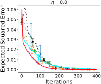
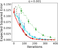
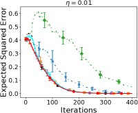
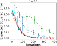
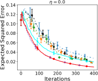
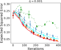
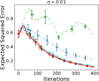
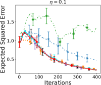
Figure 1: Result of the error $E_{T}$ in the synthetic data experiments with $\eta=0,0.001,0.01,0.1$. The horizontal and vertical axes show the number of iterations and $E_{T}$, respectively. The error bar shows mean and standard errors for 20 random trials regarding the random initial point (and the algorithm’s randomness). The top and bottom columns represent the results of the SE and Matérn kernels, respectively.

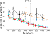
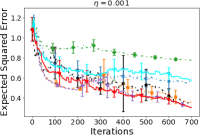
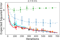
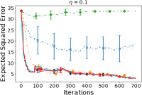
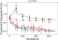
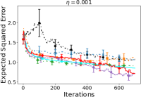
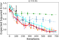
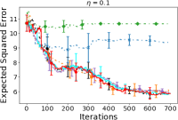
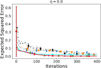
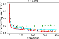
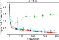
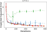
Figure 2: Result of the error $E_{T}$ in the real-world data experiments with $\eta=0,0.001,0.01,0.1$. The horizontal and vertical axes show the number of iterations and $E_{T}$, respectively. The error bar shows mean and standard errors for 20 random trials regarding the random initial point (and the algorithm’s randomness). The top, middle, and bottom columns represent the results of the King County house sales dataset, red wine quality dataset, and auto MPG dataset, respectively.

6 Experiments

In this section, we demonstrate the effectiveness of the proposed methods via synthetic and real-world datasets. We employ RS, US, variance reduction (Yu et al., 2006), and expected predictive information gain (EPIG) (Bickford Smith et al., 2023) as the baseline. We show the implementation details of EPIG in Appendix C.2. Furthermore, as the ablation study, we performed the method, referred to as DR variance reduction, that greedily minimizes $E_{p_{t}(\boldsymbol{x}^{*})}\left[\sigma^{2}_{t}(\boldsymbol{x}^{*}\mid\boldsymbol{x})\right]$, that is, the unconstrained version of Eq. (4). We referred to the proposed methods as DR random and constrained DR variance reduction (CDR variance reduction). We evaluate the performance by the error $E_{T}$ defined in Eq. (2). Furthermore, for the synthetic dataset, we show the result of $\max_{p\in{\cal P}}\mathbb{E}_{p(\boldsymbol{x})}\left[\sigma_{t}^{2}(\boldsymbol{x})\mid{\cal D}_{t}\right]$ in Appendix C.1.

In these experiments, by some $\eta\geq 0$, we define the ambiguity set as follows:

$${\cal P}=\{p\in{\cal P}_{{\cal X}}\mid\|p_{\rm ref}-p\|_{\infty}\leq\eta\},$$

where ${\cal P}_{{\cal X}}$ and $p_{\rm ref}$ are sets of all distributions over ${\cal X}$ and some reference distribution, respectively, and $\|\cdot\|_{\infty}$ denotes $L_{\infty}$ norm. Note that $\eta=0$ matches the case that the unique target distribution $p_{\rm ref}$ is specified. Since we consider the case of discrete ${\cal X}$, maximization over ${\cal P}$ can be written as linear programming for which we used CVXPY (Diamond and Boyd, 2016; Agrawal et al., 2018).

6.1 Synthetic Data Experiemnts

We set ${\cal X}=\{-1,-0.8,\ldots,1\}^{3}$, where $|{\cal X}|=11^{3}=1331$. The target function $f$ is the sample path from GPs, where we use SE and Matérn-$\nu$ kernels with $\nu=5/2$. We use the fixed hyperparameters of the kernel function in the GPR model, which is used to generate $f$, and fix $\sigma^{2}=10^{-4}$. The first input $\boldsymbol{x}_{1}$ is selected by uniformly random, and $T$ is set as $400$. Furthermore, we set $p_{\rm ref}={\cal N}(\boldsymbol{0},0.2\boldsymbol{I}_{3})$.

Figures 1 shows the result. We can see that DR and CDR variance reductions show superior performance consistently for all the kernel functions and $\eta$, although the DR random is often inferior to those due to the randomness. This result suggests that the DR and CDR variance reductions effectively incorporate the information of ${\cal P}$. Furthermore, although the constraint by ${\cal X}_{t}$ is required for the theoretical analysis in CDR variance reduction, we can confirm that it does not sacrifice the practical effectiveness. On the other hand, the usual AL methods, such as US and variance reduction, deteriorate when $\eta$ is small since they do not incorporate the information of ${\cal P}$. When $\eta$ is large since our problem approaches the worst-case error minimization, the US and variance reduction result in relatively good results. On the other hand, the EPIG designed for the case $\eta=0$ is inferior for all $\eta$ since the EPIG is based on the entropy ${\cal O}\left(\log(\sigma_{t}(\boldsymbol{x}))\right)$, not the squared error. That is, since $\frac{\partial\log a}{\partial a}=\frac{1}{a}$ is large when $a\rightarrow 0$, the EPIG tends to make a small $\sigma_{t}(\boldsymbol{x})$ more small than making a large $\sigma_{t}(\boldsymbol{x})$ small.

6.2 Real-World Dataset Experiments

We use the King County house sales, the red wine quality (Cortez and Reis, 2009), and the auto MPG datasets (Quinlan, 1993) (See Appendix C.3 for details). For all experiments, we used SE kernels, where the hyperparameters $\ell$, and $\sigma^{2}$ are adaptively determined by the marginal likelihood maximization (Rasmussen and Williams, 2005) per 10 iterations. The first input is selected uniformly random. Furthermore, we normalize the inputs and outputs of all datasets before the experiments and set $p_{\rm ref}={\cal N}(\boldsymbol{0},0.3\boldsymbol{I}_{d})$.

Figure 2 shows the result. We can confirm the same tendency that DR and CDR variance reductions show superior performance consistently as the synthetic data experiments shown in Figure 1. Note that the fluctuations come from the hyperparameter estimation.

7 Conclusion

This paper investigated the DRAL problem for the GPR, in which we aim to reduce the worst-case error $E_{T}$. We first showed several properties of this problem for the GPR, which implies that minimizing the variance guarantees a decrease in $E_{T}$. Therefore, we designed two algorithms that reduce the target variance and incorporate information about target distribution candidates for practical effectiveness. Then, we proved the theoretical error convergence of the proposed methods, whose practical effectiveness is demonstrated via synthetic and real-world datasets.

Limitation and Future Work:

We can consider several future research directions. First, since we do not show the optimality of the convergence rate, developing a (near) optimal algorithm for $E_{T}$ is vital. For this goal, the approximate submodularity (Bian et al., 2017) may be relevant from the empirical superiority of DR variance reduction. Second, since the expectation over $p(\boldsymbol{x}^{*})$ may be intractable, an analysis incorporating the approximation error or developing an algorithm that is efficient without expectation computation may be crucial (DR random does not require the expectation but is often inefficient). Third, although our analyses only require the existence of the maximum over ${\cal P}$, our experiments are limited to the discrete distribution set defined by $L_{\infty}$ ball. Thus, more general experiments regarding, e.g., the continuous probability distributions and the ambiguity sets defined by Kullback-Leibler divergence (Hu and Hong, 2013) and Wasserstein distance (Frogner et al., 2021), are interesting from the practical perspective.

Acknowkedgements

This work was partially supported by JST ACT-X Grant Number (JPMJAX23CD and JPMJAX24C3), JST PRESTO Grant Number JPMJPR24J6, JST CREST Grant Numbers (JPMJCR21D3 including AIP challenge program and JPMJCR22N2), JST Moonshot R&D Grant Number JPMJMS2033-05, JSPS KAKENHI Grant Number (JP20H00601, JP23K16943, JP23K19967, JP24K15080, and JP24K20847), NEDO (JPNP20006), and RIKEN Center for Advanced Intelligence Project.

Appendix A Proofs for Section 3

A.1 Proof of Lemma 3.2

From the definition of $\mu_{t}$, we obtain

$$\mu_{t}(\cdot) \leq\boldsymbol{v}_{t}^{\top}(\cdot)\boldsymbol{y}_{t}$$

$$\leq\boldsymbol{v}_{t}^{\top}(\cdot)\boldsymbol{f}_{t}+\boldsymbol{v}_{t}^{\top}(\cdot)\boldsymbol{\epsilon}_{t},$$

where $\boldsymbol{v}_{t}(\boldsymbol{x})=\left(\boldsymbol{k}_{t}^{\top}(\boldsymbol{x})(\boldsymbol{K}_{t}+\sigma^{2}\boldsymbol{I}_{t})^{-1}\right)^{\top}$, $\boldsymbol{f}_{t}=\bigl{(}f(\boldsymbol{x}_{1}),\dots,f(\boldsymbol{x}_{t})\bigr{)}^{\top}$, and $\boldsymbol{\epsilon}_{t}=(\epsilon_{1},\dots,\epsilon_{t})^{\top}$. Therefore, the Lipschitz constant of $\mu_{t}$ is bounded from above by the Lipscthiz constants of $\boldsymbol{v}_{t}^{\top}(\cdot)\boldsymbol{f}_{t}$ and $\boldsymbol{v}_{t}^{\top}(\cdot)\boldsymbol{\epsilon}_{t}$.

For the first term $\boldsymbol{v}_{t}^{\top}(\cdot)\boldsymbol{f}_{t}$, we follow the proof of Lemma 4 of Vakili et al. [2021a]. Recall the RKHS-based definition of kernel ridge estimator:

$$\mu_{t}=\operatorname*{arg\,min}_{\mu\in{\cal H}_{k}}\sum_{i=1}^{t}\bigl{(}y_{\boldsymbol{x}_{i}}-\mu(\boldsymbol{x}_{i})\bigr{)}^{2}+\sigma^{2}\|\mu\|_{{\cal H}_{k}}.$$

Therefore, we can derive

$$\min_{\mu\in{\cal H}_{k}}\sum_{i=1}^{t}\bigl{(}f(\boldsymbol{x}_{i})-\mu(\boldsymbol{x}_{i})\bigr{)}^{2}+\sigma^{2}\|\mu\|_{{\cal H}_{k}} =\sum_{i=1}^{t}\bigl{(}f(\boldsymbol{x}_{i})-\boldsymbol{v}_{t}^{\top}(\boldsymbol{x}_{i})\boldsymbol{f}_{t}\bigr{)}^{2}+\sigma^{2}\|\boldsymbol{v}_{t}^{\top}(\cdot)\boldsymbol{f}_{t}\|_{{\cal H}_{k}}$$

$$\leq\sum_{i=1}^{t}\bigl{(}f(\boldsymbol{x}_{i})-f(\boldsymbol{x}_{i})\bigr{)}^{2}+\sigma^{2}\|f\|_{{\cal H}_{k}} \left(\because f\in{\cal H}_{k}\right)$$

$$=\sigma^{2}\|f\|_{{\cal H}_{k}}.$$

Hence, we obtain $\|\boldsymbol{v}_{t}^{\top}(\cdot)\boldsymbol{f}_{t}\|_{{\cal H}_{k}}\leq\|f\|_{{\cal H}_{k}}\leq B$. By combining Lemma 2.9, $\boldsymbol{v}_{t}^{\top}(\cdot)\boldsymbol{f}_{t}$ is $BL_{k}$ Lipschitz continuous.

For the second term $\boldsymbol{v}_{t}^{\top}(\cdot)\boldsymbol{\epsilon}_{t}$, we leverage the confidence bounds of kernel ridge estimator [Theorem 3.11 in Abbasi-Yadkori, 2013]. Let $g:{\cal X}\times\{0,1\}\rightarrow\mathbb{R}$ as $g(\boldsymbol{x},0)=g(\boldsymbol{x},1)=0$ and fix $j\in[d]$. Then, the zero function $g$ belongs to the RKHS with any kernel function $\overline{k}$. Thus, we design the following kernel function $\overline{k}$:

$$\overline{k}\left((\boldsymbol{x},0),(\boldsymbol{z},0)\right) =k(\boldsymbol{x},\boldsymbol{z}),$$

$$\overline{k}\left((\boldsymbol{x},1),(\boldsymbol{z},1)\right) =\frac{\partial^{2}k(\boldsymbol{x},\boldsymbol{z})}{\partial x_{j}\partial z_{j}},$$

$$\overline{k}\left((\boldsymbol{x},0),(\boldsymbol{z},1)\right) =\frac{\partial k(\boldsymbol{x},\boldsymbol{z})}{\partial z_{j}},$$

for all $\boldsymbol{x},\boldsymbol{z}\in{\cal X}$. Note that since the kernel function, $k$ has partial derivatives due to Assumption 2.8, the derivative of the kernel and the kernel itself are the kernels again as discussed in, e.g., Sec. 9.4 in Rasmussen and Williams [2005] and Sec. 2.2 in Adler [1981]. Thus, we can interpret $\overline{\boldsymbol{v}}_{t}^{\top}(\cdot)\boldsymbol{\epsilon}_{t}$ as the kernel ridge estimator for $g(\boldsymbol{x},1)$, where $\overline{\boldsymbol{v}}_{t}(\boldsymbol{x})=\left(\frac{\partial\boldsymbol{k}_{t}^{\top}(\boldsymbol{x})}{\partial x_{j}}(\boldsymbol{K}_{t}+\sigma^{2}\boldsymbol{I}_{t})^{-1}\right)^{\top}$. In addition, $\|g\|_{{\cal H}_{\overline{k}}}=0$. Therefore, from Theorem 3.11 in Abbasi-Yadkori [2013] and $|g(\boldsymbol{x},1)-\overline{\boldsymbol{v}}_{t}^{\top}(\boldsymbol{x})\boldsymbol{\epsilon}_{t}|=|\overline{\boldsymbol{v}}_{t}^{\top}(\boldsymbol{x})\boldsymbol{\epsilon}_{t}|$, we obtain

$$\Pr\left(|\overline{\boldsymbol{v}}_{t}^{\top}(\boldsymbol{x})\boldsymbol{\epsilon}_{t}|\leq\overline{\sigma}_{t}(\boldsymbol{x})\frac{R}{\sigma}\sqrt{2\gamma_{t}+2\log\left(1/\delta\right)},\forall\boldsymbol{x}\in{\cal X}\right)\geq 1-\delta,$$

where $\delta\in(0,1)$ and $\overline{\sigma}_{t}(\boldsymbol{x})=\overline{k}\left((\boldsymbol{x},1),(\boldsymbol{x},1)\right)-\frac{\partial\boldsymbol{k}_{t}^{\top}(\boldsymbol{x})}{\partial x_{j}}(\boldsymbol{K}_{t}+\sigma^{2}\boldsymbol{I}_{t})^{-1}\frac{\partial\boldsymbol{k}_{t}(\boldsymbol{x})}{\partial x_{j}}$ is the posterior variance that corresponds to this kernel ridge estimation. Note that since the kernel matrix $\boldsymbol{K}_{t}$ is defined by $k(\boldsymbol{x},\boldsymbol{z})$, the MIG is the usual one defined by ${\cal X}$ and $t$. In addition, due to the monotonic decreasing property of the posterior variance, $\overline{\sigma}_{t}(\boldsymbol{x})\leq L_{k}$, we obtain

$$\Pr\left(|\overline{\boldsymbol{v}}_{t}^{\top}(\boldsymbol{x})\boldsymbol{\epsilon}_{t}|\leq\frac{L_{k}R}{\sigma}\sqrt{2\gamma_{t}+2\log\left(1/\delta\right)},\forall\boldsymbol{x}\in{\cal X}\right)\geq 1-\delta,$$

and thus,

$$\Pr\left(\sup_{\boldsymbol{x}\in{\cal X}}|\overline{\boldsymbol{v}}_{t}^{\top}(\boldsymbol{x})\boldsymbol{\epsilon}_{t}|\leq\frac{L_{k}R}{\sigma}\sqrt{2\gamma_{t}+2\log\left(1/\delta\right)}\right)\geq 1-\delta.$$

Consequently, by using the union bound for all $j\in[d]$, we derive

$$\Pr\left(\sup_{j\in[d]}\sup_{\boldsymbol{x}\in{\cal X}}|\overline{\boldsymbol{v}}_{t}^{\top}(\boldsymbol{x})\boldsymbol{\epsilon}_{t}|\leq\frac{L_{k}R}{\sigma}\sqrt{2\gamma_{t}+2\log\left(d/\delta\right)}\right)\geq 1-\delta,$$

which shows that $\boldsymbol{v}_{t}^{\top}(\boldsymbol{x})\boldsymbol{\epsilon}_{t}$ is $\frac{L_{k}R}{\sigma}\sqrt{2\gamma_{t}+2\log\left(d/\delta\right)}$ Lipschitz continuous.

Combining the Lipschitz constants of $\boldsymbol{v}_{t}^{\top}(\cdot)\boldsymbol{f}_{t}$ and $\boldsymbol{v}_{t}^{\top}(\cdot)\boldsymbol{\epsilon}_{t}$, we can obtain the result.

A.2 Proof of Lemma 3.3

First, we fix $(\boldsymbol{x}_{i})_{i\in[t]}$ without loss of generality since

$$\Pr\left(\sup_{\boldsymbol{x}\in{\cal X}}\left|\frac{\partial\mu_{t}(\boldsymbol{u})}{\partial u_{j}}\Big{|}_{\boldsymbol{u}=\boldsymbol{x}}\right|>L\right) =\mathbb{E}_{(\boldsymbol{x}_{i})_{i\in[t]}}\left[\Pr\left(\sup_{\boldsymbol{x}\in{\cal X}}\left|\frac{\partial\mu_{t}(\boldsymbol{u})}{\partial u_{j}}\Big{|}_{\boldsymbol{u}=\boldsymbol{x}}\right|>L\bigg{|}(\boldsymbol{x}_{i})_{i\in[t]}\right)\right].$$

That is, the upper bound of the conditional probability given any $(\boldsymbol{x}_{i})_{i\in[t]}$ directly suggests the upper bound of target probability in the left-hand side. Note that from the assumption $(\boldsymbol{x}_{i})_{i\in[t]}$ is independent of $(\epsilon_{i})_{i\in[t]}$ and $f$, the observations $\boldsymbol{y}_{t}$ follows Gaussian distribution even if $(\boldsymbol{x}_{i})_{i\in[t]}$ is fixed.

We leverage Slepian’s inequality shown as Proposition A.2.6 in van der Vaart and Wellner [1996]:

Lemma A.1 (Slepian, Fernique, Marcus, and Shepp).

Let $X$ and $Y$ be separable, mean-zero Gaussian processes indexed by a common index set $T$ such that

$$\mathbb{E}[(X_{s}-X_{t})^{2}]\leq\mathbb{E}[(Y_{s}-Y_{t})^{2}],$$

for all $s,t\in T$. Then,

$$\Pr\left(\sup_{t\in T}X_{t}\geq\lambda\right)\leq\Pr\left(\sup_{t\in T}Y_{t}\geq\lambda\right),$$

for all $\lambda>0$.

The separability [Definition 5.22 in Handel, 2016] holds commonly. As discussed in Remark 5.23 in Handel [2016], for example, if the sample path is almost surely continuous, then the separability holds. Furthermore, the sample path defined by the commonly used kernel functions, such as linear, SE, and Matérn-$\nu$ kernels with $\nu\geq 1$, is continuous almost surely [Costa et al., 2024]. In addition, if the kernel function is continuous, the posterior mean function is also continuous, almost surely.

First, we provide the proof of the result regarding $\mu_{t}(\boldsymbol{x})$. Since $\boldsymbol{y}_{t}\mid(\boldsymbol{x}_{i})_{i\in[t]}\sim{\cal N}(\boldsymbol{0},\boldsymbol{K}_{t}+\sigma^{2}\boldsymbol{I}_{t})$, we can see that $\mu_{t}\mid(\boldsymbol{x}_{i})_{i\in[t]}\sim{\cal G}{\cal P}\bigl{(}0,k_{\mu_{t}}(\boldsymbol{x},\boldsymbol{z})\bigr{)}$, where $k_{\mu_{t}}(\boldsymbol{x},\boldsymbol{z})=\boldsymbol{k}_{t}(\boldsymbol{x})^{\top}\bigl{(}\boldsymbol{K}+\sigma^{2}\boldsymbol{I}_{t}\bigr{)}^{-1}\boldsymbol{k}_{t}(\boldsymbol{z})$. Furthermore, it is known that if the kernel has mixed partial derivative $\frac{\partial^{2}k(\boldsymbol{x},\boldsymbol{z})}{\partial x_{j}\partial z_{j}}$, $f$ and its derivative $\partial f(\boldsymbol{x})/\partial x_{j}$ jointly follow GPs [Rasmussen and Williams, 2005, Adler, 1981]. Specifically, the derivative is distributed as

$$f^{(j)}\coloneqq\frac{\partial f(\boldsymbol{x})}{\partial x_{j}} \sim{\cal G}{\cal P}\left(0,\tilde{k}(\boldsymbol{x},\boldsymbol{z})\coloneqq\frac{\partial^{2}k(\boldsymbol{u},\boldsymbol{v})}{\partial u_{j}\partial v_{j}}\bigg{|}_{\boldsymbol{u}=\boldsymbol{x},\boldsymbol{v}=\boldsymbol{z}}\right),$$

for all $j\in[d]$. Note that since the prior mean of $f$ is zero, the prior mean of $f^{(j)}$ is also zero. As with $f$, the derivative of $\mu_{t}$ is distributed as

$$\mu_{t}^{(j)}\coloneqq\frac{\partial\mu_{t}(\boldsymbol{x})}{\partial x_{j}}\mid(\boldsymbol{x}_{i})_{i\in[t]} \sim{\cal G}{\cal P}\left(0,\tilde{k}_{\mu_{t}}(\boldsymbol{x},\boldsymbol{z})\coloneqq\frac{\partial^{2}k_{\mu_{t}}(\boldsymbol{u},\boldsymbol{v})}{\partial u_{j}\partial v_{j}}\bigg{|}_{\boldsymbol{u}=\boldsymbol{x},\boldsymbol{v}=\boldsymbol{z}}\right),$$

for all $j\in[d]$. In addition, the covariance is given as

$${\rm Cov}\left(f(\boldsymbol{x}),f^{(j)}(\boldsymbol{z})\right) =\frac{\partial k(\boldsymbol{x},\boldsymbol{u})}{\partial u_{j}}\bigg{|}_{\boldsymbol{u}=\boldsymbol{z}}.$$

Then, we see that the posterior variance of the derivative can be obtained in the same way as the usual GP calculation as follows:

$${\rm Var}\left(f^{(j)}(\boldsymbol{x})\mid{\cal D}_{t}\right) =\tilde{k}(\boldsymbol{x},\boldsymbol{x})-\tilde{k}_{\mu_{t}}(\boldsymbol{x},\boldsymbol{x}),$$

$${\rm Cov}\left(f^{(j)}(\boldsymbol{x}),f^{(j)}(\boldsymbol{z})\mid{\cal D}_{t}\right) =\tilde{k}(\boldsymbol{x},\boldsymbol{z})-\tilde{k}_{\mu_{t}}(\boldsymbol{x},\boldsymbol{z}).$$

On the other hand, we can obtain that

$$\mathbb{E}\left[\bigl{(}f^{(j)}(\boldsymbol{x})-f^{(j)}(\boldsymbol{z})\bigr{)}^{2}\right] =\tilde{k}(\boldsymbol{x},\boldsymbol{x})+\tilde{k}(\boldsymbol{z},\boldsymbol{z})-2\tilde{k}(\boldsymbol{x},\boldsymbol{z}),$$

$$\mathbb{E}\left[\bigl{(}\mu_{t}^{(j)}(\boldsymbol{x})-\mu_{t}^{(j)}(\boldsymbol{z})\bigr{)}^{2}\mid(\boldsymbol{x}_{i})_{i\in[t]}\right] =\tilde{k}_{\mu_{t}}(\boldsymbol{x},\boldsymbol{x})+\tilde{k}_{\mu_{t}}(\boldsymbol{z},\boldsymbol{z})-2\tilde{k}_{\mu_{t}}(\boldsymbol{x},\boldsymbol{z}),$$

for all $\boldsymbol{x},\boldsymbol{z}\in{\cal X}$. Then, we obtain

$$\mathbb{E}\left[\bigl{(}f^{(j)}(\boldsymbol{x})-f^{(j)}(\boldsymbol{z})\bigr{)}^{2}\right]-\mathbb{E}\left[\bigl{(}\mu_{t}^{(j)}(\boldsymbol{x})-\mu_{t}^{(j)}(\boldsymbol{z})\bigr{)}^{2}\mid(\boldsymbol{x}_{i})_{i\in[t]}\right]$$

$$=\tilde{k}(\boldsymbol{x},\boldsymbol{x})+\tilde{k}(\boldsymbol{z},\boldsymbol{z})-2\tilde{k}(\boldsymbol{x},\boldsymbol{z})-\left(\tilde{k}_{\mu_{t}}(\boldsymbol{x},\boldsymbol{x})+\tilde{k}_{\mu_{t}}(\boldsymbol{z},\boldsymbol{z})-2\tilde{k}_{\mu_{t}}(\boldsymbol{x},\boldsymbol{z})\right)$$

$$={\rm Var}\left(f^{(j)}(\boldsymbol{x})\mid{\cal D}_{t}\right)+{\rm Var}\left(f^{(j)}(\boldsymbol{z})\mid{\cal D}_{t}\right)-2{\rm Cov}\left(f^{(j)}(\boldsymbol{x}),f^{(j)}(\boldsymbol{z})\mid{\cal D}_{t}\right)\geq 0.$$

Consequently, by applying Lemma A.1, we obtain

$$\Pr\left(\sup_{\boldsymbol{x}\in{\cal X}}\mu^{(j)}_{t}(\boldsymbol{x})\geq\lambda\biggm{|}(\boldsymbol{x}_{i})_{i\in[t]}\right)\leq\Pr\left(\sup_{\boldsymbol{x}\in{\cal X}}f^{(j)}_{t}(\boldsymbol{x})\geq\lambda\right).$$

Since $\mu^{(j)}_{t}(\boldsymbol{x})$ and $f^{(j)}_{t}(\boldsymbol{x})$ follow centered GPs, we obtain

$$\Pr\left(\sup_{\boldsymbol{x}\in{\cal X}}\left|\mu^{(j)}_{t}(\boldsymbol{x})\right|\geq\lambda\biggm{|}(\boldsymbol{x}_{i})_{i\in[t]}\right)\leq 2\Pr\left(\sup_{\boldsymbol{x}\in{\cal X}}\mu^{(j)}_{t}(\boldsymbol{x})\geq\lambda\biggm{|}(\boldsymbol{x}_{i})_{i\in[t]}\right)\leq 2\Pr\left(\sup_{\boldsymbol{x}\in{\cal X}}\left|f^{(j)}_{t}(\boldsymbol{x})\right|\geq\lambda\right).$$

Hence, from Lemma 2.5, we obtain the desired result.

We can obtain the result regarding $f^{(j)}(\boldsymbol{x})-\mu_{t}^{(j)}(\boldsymbol{x})$ in almost the same proof. We can see that

$$f^{(j)}(\boldsymbol{x})-\mu_{t}^{(j)}(\boldsymbol{x})\sim{\cal G}{\cal P}(0,\tilde{k}(\boldsymbol{x},\boldsymbol{z})-\tilde{k}_{\mu_{t}}(\boldsymbol{x},\boldsymbol{z})).$$

Then,

$$\mathbb{E}\left[\bigl{(}f^{(j)}(\boldsymbol{x})-f^{(j)}(\boldsymbol{z})\bigr{)}^{2}\right]-\mathbb{E}\left[\left(f^{(j)}(\boldsymbol{x})-\mu_{t}^{(j)}(\boldsymbol{x})-\bigl{(}f^{(j)}(\boldsymbol{x})-\mu_{t}^{(j)}(\boldsymbol{x})\bigr{)}\right)^{2}\biggm{|}(\boldsymbol{x}_{i})_{i\in[t]}\right]$$

$$=\tilde{k}_{\mu_{t}}(\boldsymbol{x},\boldsymbol{x})+\tilde{k}_{\mu_{t}}(\boldsymbol{z},\boldsymbol{z})-2\tilde{k}_{\mu_{t}}(\boldsymbol{x},\boldsymbol{z})\geq 0.$$

Remained proof is the same as the case of $\mu_{t}^{(j)}$.

A.3 Proof of Lemma 3.4

As with the existing studies [e.g., Srinivas et al., 2010], we consider the discretization of input space. Let $\overline{{\cal X}}\subset{\cal X}$ be a finite set with each dimension equally divided into $\lceil\tau dr\rceil$, where $\tau>0$. Therefore, $|\overline{{\cal X}}|=\lceil\tau dr\rceil^{d}$ and $\sup_{\boldsymbol{x}\in{\cal X}}\|\boldsymbol{x}-[\boldsymbol{x}]\|_{1}\leq\frac{1}{\tau}$, where $[\boldsymbol{x}]$ is the nearest input in $\overline{{\cal X}}$, that is, $[\boldsymbol{x}]=\operatorname*{arg\,min}_{\tilde{\boldsymbol{x}}\in\overline{{\cal X}}}\|\tilde{\boldsymbol{x}}-\boldsymbol{x}\|_{1}$. Note that we leverage $\overline{{\cal X}}$ purely sake for the analysis, and $\overline{{\cal X}}$ is not related to the algorithm.

From Assumption 2.8 and Lemma 2.9, we see that $f$ is $BL_{k}$ Lipschitz continuous. Furthermore, from Lemma 3.2, $\mu_{t}$ is $L_{k}\left(B+\frac{R}{\sigma}\sqrt{2\gamma_{t}+2\log\left(\frac{d}{\delta}\right)}\right)$ Lipschitz continuous with probability at least $1-\delta$. Combining the above, we see that $f-\mu_{t}$ is $L_{k}\left(2B+\frac{R}{\sigma}\sqrt{2\gamma_{t}+2\log\left(\frac{d}{\delta}\right)}\right)$ Lipschitz continuous with probability at least $1-\delta$.

From the above arguments, by combining Lemma 2.10 and the union bound, the following events hold simultaneously with probability at least $1-\delta$:

1. $f(\boldsymbol{x})-\mu_{T}(\boldsymbol{x})$ is $L_{\rm res}(T)$ Lipschitz continuous, where $L_{\rm res}(T)=L_{k}\left(2B+\frac{R}{\sigma}\sqrt{2\gamma_{T}+2\log\left(\frac{2d}{\delta}\right)}\right)$.

2. The confidence bounds on $\overline{{\cal X}}$ hold; that is,

   $$\forall\boldsymbol{x}\in\overline{{\cal X}},|f(\boldsymbol{x})-\mu_{T}(\boldsymbol{x})|\leq\beta_{\delta,\tau}^{1/2}\sigma_{T}(\boldsymbol{x}),$$

   where $\beta_{\delta,\tau}=\left(B+\frac{R}{\sigma}\sqrt{2d\log\left(\tau dr+1\right)+2\log\left(\frac{4}{\delta}\right)}\right)^{2}$.

Then, we can obtain the upper bound as follows:

$$E_{T} =\max_{p\in{\cal P}}\mathbb{E}_{p(\boldsymbol{x}^{*})}\left[\left(f(\boldsymbol{x}^{*})-\mu_{T}(\boldsymbol{x}^{*})\right)^{2}\right]$$

$$\leq\max_{p\in{\cal P}}\mathbb{E}_{p(\boldsymbol{x}^{*})}\left[\left(f([\boldsymbol{x}^{*}])-\mu_{T}([\boldsymbol{x}^{*}])+L_{\rm res}(T)\|\boldsymbol{x}^{*}-[\boldsymbol{x}^{*}]\|_{1}\right)^{2}\right] \left(\because\text{The above event~1}\right)$$

$$\leq\max_{p\in{\cal P}}\mathbb{E}_{p(\boldsymbol{x}^{*})}\left[\left(f([\boldsymbol{x}^{*}])-\mu_{T}([\boldsymbol{x}^{*}])+\frac{L_{\rm res}(T)}{\tau}\right)^{2}\right] \left(\because\text{The definition of $\overline{{\cal X}}$}\right)$$

$$\leq\max_{p\in{\cal P}}\mathbb{E}_{p(\boldsymbol{x}^{*})}\left[\left(\beta_{\delta,\tau}^{1/2}\sigma_{T}([\boldsymbol{x}^{*}])+\frac{L_{\rm res}(T)}{\tau}\right)^{2}\right] \left(\because\text{The above event~2}\right)$$

$$\leq\max_{p\in{\cal P}}\mathbb{E}_{p(\boldsymbol{x}^{*})}\left[\left(\beta_{\delta,\tau}^{1/2}\sigma_{T}(\boldsymbol{x}^{*})+\frac{\beta_{\delta,\tau}^{1/2}L_{\sigma}+L_{\rm res}(T)}{\tau}\right)^{2}\right] \left(\because\text{Lemma~\ref{lem:Lipschitz_posterior_var}}\right)$$

$$\leq 2\beta_{\delta,\tau}\max_{p\in{\cal P}}\mathbb{E}_{p(\boldsymbol{x}^{*})}\left[\sigma_{T}^{2}(\boldsymbol{x}^{*})\right]+2\left(\frac{\beta_{\delta,\tau}^{1/2}L_{\sigma}+L_{\rm res}(T)}{\tau}\right)^{2}. \left(\because(a+b)^{2}/2\leq a^{2}+b^{2}\right)$$

If we set $\tau=T$, noting that $L_{\rm res}(T)={\cal O}(\sqrt{\gamma_{T}})$ and $\beta_{\delta,\tau}^{1/2}={\cal O}(\log(T/\delta))$, we obtain the following:

$$E_{T} \leq 2\beta_{\delta,T}\max_{p\in{\cal P}}\mathbb{E}_{p(\boldsymbol{x}^{*})}\left[\sigma_{T}^{2}(\boldsymbol{x}^{*})\right]+{\cal O}\left(\frac{\max\{\gamma_{T},\log(T/\delta)\}}{T^{2}}\right).$$

Although by setting $\tau=\Omega(T)$, we can make the second term small arbitrarily, $\beta_{\delta,T}=\Theta\left(\log(T/\delta)\right)$ and $\mathbb{E}_{p(\boldsymbol{x}^{*})}\left[\sigma_{T}^{2}(\boldsymbol{x}^{*})\right]=\Omega(1/T)$ [Lemma 4.2 in Takeno et al., 2024]. Therefore, since the first term is $\Omega\left(\frac{\log(T/\delta)}{T}\right)$ and $\frac{\max\{\gamma_{T},\log(T/\delta)\}}{T^{2}}={\cal O}\left(\frac{\log(1/\delta)}{T}\right)$ if $\gamma_{T}$ is sublinear, we do not set $\tau$ more large value for simplicity.

A.4 Proof of Lemma 3.5

As with the existing studies [e.g., Srinivas et al., 2010], we consider the discretization of input space. Let $\overline{{\cal X}}\subset{\cal X}$ be a finite set with each dimension equally divided into $\lceil\tau dr\rceil$, where $\tau>0$. Therefore, $|\overline{{\cal X}}|=\lceil\tau dr\rceil^{d}$ and $\sup_{\boldsymbol{x}\in{\cal X}}\|\boldsymbol{x}-[\boldsymbol{x}]\|_{1}\leq\frac{1}{\tau}$, where $[\boldsymbol{x}]$ is the nearest input in $\overline{{\cal X}}$, that is, $[\boldsymbol{x}]=\operatorname*{arg\,min}_{\tilde{\boldsymbol{x}}\in\overline{{\cal X}}}\|\tilde{\boldsymbol{x}}-\boldsymbol{x}\|_{1}$. Note that we leverage $\overline{{\cal X}}$ purely sake for the analysis, and $\overline{{\cal X}}$ is not related to the algorithm.

In addition, from Lemma 3.3, the following inequality holds with probability at least $1-\delta$:

$$\sup_{j\in d}\sup_{\boldsymbol{x}\in{\cal X}}\left|\frac{\partial r_{t}(\boldsymbol{u})}{\partial u_{j}}\Big{|}_{\boldsymbol{u}=\boldsymbol{x}}\right|\leq b\sqrt{\log(2ad/\delta)},$$

which implies that $L_{\rm res}$, the Lipschitz constant of $r_{t}(\boldsymbol{x})=f(\boldsymbol{x})-\mu_{T}(\boldsymbol{x})$, can be bounded from above.

Then, by combining the above argument, Lemma 2.6, and the union bound, the following events hold simultaneously with probability at least $1-\delta$:

1. $f(\boldsymbol{x})-\mu_{T}(\boldsymbol{x})$ is $L_{\rm res}$ Lipschitz continuous, where $L_{\rm res}=b\sqrt{\log(4ad/\delta)}$.

2. The confidence bounds on $\overline{{\cal X}}$ hold; that is,

   $$\forall\boldsymbol{x}\in\overline{{\cal X}},|f(\boldsymbol{x})-\mu_{T}(\boldsymbol{x})|\leq\beta_{\delta,\tau}^{1/2}\sigma_{T}(\boldsymbol{x}),$$

   where $\beta_{\delta,\tau}=2d\log(\tau dr+1)+2\log(2/\delta)$.

Hence, we can obtain the upper bound as follows:

$$E_{T} =\max_{p\in{\cal P}}\mathbb{E}_{p(\boldsymbol{x}^{*})}\left[\left(f(\boldsymbol{x}^{*})-\mu_{T}(\boldsymbol{x}^{*})\right)^{2}\right]$$

$$\leq\max_{p\in{\cal P}}\mathbb{E}_{p(\boldsymbol{x}^{*})}\left[\left(f([\boldsymbol{x}^{*}])-\mu_{T}([\boldsymbol{x}^{*}])+L_{\rm res}\|\boldsymbol{x}^{*}-[\boldsymbol{x}^{*}]\|_{1}\right)^{2}\right] \left(\because\text{The above event~1}\right)$$

$$\leq\max_{p\in{\cal P}}\mathbb{E}_{p(\boldsymbol{x}^{*})}\left[\left(f([\boldsymbol{x}^{*}])-\mu_{T}([\boldsymbol{x}^{*}])+\frac{L_{\rm res}}{\tau}\right)^{2}\right] \left(\because\text{The definition of $\overline{{\cal X}}$}\right)$$

$$\leq\max_{p\in{\cal P}}\mathbb{E}_{p(\boldsymbol{x}^{*})}\left[\left(\beta_{\delta,\tau}^{1/2}\sigma_{T}([\boldsymbol{x}^{*}])+\frac{L_{\rm res}}{\tau}\right)^{2}\right] \left(\because\text{The above event~2}\right)$$

$$\leq\max_{p\in{\cal P}}\mathbb{E}_{p(\boldsymbol{x}^{*})}\left[\left(\beta_{\delta,\tau}^{1/2}\sigma_{T}(\boldsymbol{x}^{*})+\frac{\beta_{\delta,\tau}^{1/2}L_{\sigma}+L_{\rm res}}{\tau}\right)^{2}\right] \left(\because\text{Lemma~\ref{lem:Lipschitz_posterior_var}}\right)$$

$$\leq 2\beta_{\delta,\tau}\max_{p\in{\cal P}}\mathbb{E}_{p(\boldsymbol{x}^{*})}\left[\sigma_{T}^{2}(\boldsymbol{x}^{*})\right]+2\left(\frac{\beta_{\delta,\tau}^{1/2}L_{\sigma}+L_{\rm res}}{\tau}\right)^{2}. \left(\because(a+b)^{2}/2\leq a^{2}+b^{2}\right)$$

Then, by setting $\tau=T$, we can see that

$$E_{T} \leq 2\beta_{\delta,T}\max_{p\in{\cal P}}\mathbb{E}_{p(\boldsymbol{x}^{*})}\left[\sigma_{T}^{2}(\boldsymbol{x}^{*})\right]+{\cal O}\left(\frac{\log(T/\delta)}{T^{2}}\right).$$

Although by setting $\tau=\Omega(T)$, we can make the second term small arbitrarily, we do not do so since the first term is dominant compared with ${\cal O}\left(\frac{\log(T/\delta)}{T^{2}}\right)$ term.

A.5 Proof of Lemma 3.6

Since the maximum $\tilde{p}_{T}(\boldsymbol{x}^{*})=\operatorname*{arg\,max}_{p\in{\cal P}}\mathbb{E}_{p(\boldsymbol{x}^{*})}\left[|f(\boldsymbol{x}^{*})-\mu_{T}(\boldsymbol{x}^{*})|\right]$ exists, we obtain

$$\max_{p\in{\cal P}}\mathbb{E}_{p(\boldsymbol{x}^{*})}\left[|f(\boldsymbol{x}^{*})-\mu_{T}(\boldsymbol{x}^{*})|\right] =\mathbb{E}_{\tilde{p}_{T}(\boldsymbol{x}^{*})}\left[|f(\boldsymbol{x}^{*})-\mu_{T}(\boldsymbol{x}^{*})|\right],$$

$$\leq\sqrt{\mathbb{E}_{\tilde{p}_{T}(\boldsymbol{x}^{*})}\left[(f(\boldsymbol{x}^{*})-\mu_{T}(\boldsymbol{x}^{*}))^{2}\right]},$$

$$\leq\sqrt{\max_{p\in{\cal P}}\mathbb{E}_{p(\boldsymbol{x}^{*})}\left[(f(\boldsymbol{x}^{*})-\mu_{T}(\boldsymbol{x}^{*}))^{2}\right]},$$

where we used Jensen’s inequality.

A.6 Proof of Lemma 3.7

Since the maximum $\overline{p}_{T}(\boldsymbol{x}^{*})=\operatorname*{arg\,max}_{p\in{\cal P}}\mathbb{E}_{p(\boldsymbol{x}^{*})}\left[H[f(\boldsymbol{x})\mid{\cal D}_{t}]\right]$ exists, we obtain

$$\max_{p\in{\cal P}}\mathbb{E}_{p(\boldsymbol{x})}[H[f(\boldsymbol{x})\mid{\cal D}_{t}]] =\frac{1}{2}\mathbb{E}_{\overline{p}_{T}(\boldsymbol{x}^{*})}[\log(2\pi e\sigma_{T}^{2}(\boldsymbol{x}))]$$

$$\leq\frac{1}{2}\log(2\pi e\mathbb{E}_{\overline{p}_{T}(\boldsymbol{x}^{*})}[\sigma_{T}^{2}(\boldsymbol{x})]) (\because\text{Jensen's inequality})$$

$$\leq\frac{1}{2}\log\left(2\pi e\max_{p\in{\cal P}}\mathbb{E}_{p(\boldsymbol{x})}[\sigma_{T}^{2}(\boldsymbol{x})]\right).$$

Appendix B Proofs for Section 4

B.1 Proof of Theorem 4.1

From the definition, $\sigma_{t}^{2}(\boldsymbol{x})$ is monotonically decreasing along with ${\cal D}_{t-1}\subset{\cal D}_{t}$. Therefore, for all $t\leq T$ and $\boldsymbol{x}_{1},\dots,\boldsymbol{x}_{T}$,

$$\max_{p\in{\cal P}}\mathbb{E}_{p(\boldsymbol{x}^{*})}[\sigma_{T}^{2}(\boldsymbol{x}^{*})\mid\boldsymbol{x}_{1},\dots,\boldsymbol{x}_{T}]\leq\max_{p\in{\cal P}}\mathbb{E}_{p(\boldsymbol{x}^{*})}[\sigma_{t}^{2}(\boldsymbol{x}^{*})\mid\boldsymbol{x}_{1},\dots,\boldsymbol{x}_{t}].$$

Note that $\boldsymbol{x}_{1},\dots,\boldsymbol{x}_{T}$ are random variables due to the randomness of the algorithm. Hence, we obtain

$$\max_{p\in{\cal P}}\mathbb{E}_{p(\boldsymbol{x}^{*})}[\sigma_{T}^{2}(\boldsymbol{x}^{*})\mid\boldsymbol{x}_{1},\dots,\boldsymbol{x}_{T}] \leq\frac{1}{T}\sum_{t=1}^{T}\max_{p\in{\cal P}}\mathbb{E}_{p(\boldsymbol{x}^{*})}[\sigma_{t-1}^{2}(\boldsymbol{x}^{*})\mid\boldsymbol{x}_{1},\dots,\boldsymbol{x}_{t-1}]$$

$$\leq\frac{1}{T}\sum_{t=1}^{T}\mathbb{E}_{p_{t}(\boldsymbol{x}_{t})}[\sigma_{t-1}^{2}(\boldsymbol{x}_{t})\mid\boldsymbol{x}_{1},\dots,\boldsymbol{x}_{t-1}]. (\because\text{Definition of $p_{t}$})$$

Then, we apply the following lemma [Lemma 3 in Kirschner and Krause, 2018]:

Lemma B.1.

Let $Y_{t}$ be any non-negative stochastic process adapted to a filtration $\{{\cal F}_{t}\}$, and define $m_{t}=\mathbb{E}[Y_{t}\mid{\cal F}_{t-1}]$. Further assume that $Y_{t}\leq b_{t}$ for a fixed, non-decreasing sequence $(b_{t})_{t\geq 1}$. Then, if $b_{T}\geq 1$, with probability at least $1-\delta$ for any $T\geq 1$, it holds that,

$$\sum_{t=1}^{T}m_{t}\leq 2\sum_{t=1}^{T}Y_{t}+4b_{T}\log\frac{1}{\delta}+8b_{T}\log(4b_{T})+1.$$

The random variable $\mathbb{E}_{p_{t}(\boldsymbol{x})}[\sigma_{t}^{2}(\boldsymbol{x})\mid\boldsymbol{x}_{1},\dots,\boldsymbol{x}_{t}]$ satisfies the condition of this lemma by setting $b_{t}=1$ for all $t\in[T]$. Therefore, with probability at least $1-\delta$,

$$\max_{p\in{\cal P}}\mathbb{E}_{p(\boldsymbol{x}^{*})}[\sigma_{T}^{2}(\boldsymbol{x}^{*})\mid\boldsymbol{x}_{1},\dots,\boldsymbol{x}_{T}] \leq\frac{1}{T}\left(2\sum_{t=1}^{T}\sigma_{t-1}^{2}(\boldsymbol{x}_{t})+4\log\frac{1}{\delta}+8\log(4)+1\right)$$

$$\leq\frac{1}{T}\left(2C_{1}\gamma_{T}+4\log\frac{1}{\delta}+8\log(4)+1\right).$$

Here, we use $\sum_{t=1}^{T}\sigma_{t-1}^{2}(\boldsymbol{x}_{t})\leq C_{1}\gamma_{T}$ [Lemma 5.2 in Srinivas et al., 2010].

B.2 Proof of Theorem 4.2

From the definition, $\sigma_{t}^{2}(\boldsymbol{x})$ is monotonically decreasing along with ${\cal D}_{t-1}\subset{\cal D}_{t}$. Therefore, for all $t\leq T$ and $\boldsymbol{x}_{1},\dots,\boldsymbol{x}_{T}$,

$$\max_{p\in{\cal P}}\mathbb{E}_{p(\boldsymbol{x}^{*})}[\sigma_{T}^{2}(\boldsymbol{x}^{*})\mid\boldsymbol{x}_{1},\dots,\boldsymbol{x}_{T}]\leq\max_{p\in{\cal P}}\mathbb{E}_{p(\boldsymbol{x}^{*})}[\sigma_{t}^{2}(\boldsymbol{x}^{*})\mid\boldsymbol{x}_{1},\dots,\boldsymbol{x}_{t}].$$

Hence, we obtain

$$\max_{p\in{\cal P}}\mathbb{E}_{p(\boldsymbol{x}^{*})}[\sigma_{T}^{2}(\boldsymbol{x}^{*})\mid\boldsymbol{x}_{1},\dots,\boldsymbol{x}_{T}] \leq\frac{1}{T}\sum_{t=1}^{T}\max_{p\in{\cal P}}\mathbb{E}_{p(\boldsymbol{x}^{*})}[\sigma_{t-1}^{2}(\boldsymbol{x}^{*})\mid\boldsymbol{x}_{1},\dots,\boldsymbol{x}_{t-1}]$$

$$\leq\frac{1}{T}\sum_{t=1}^{T}\sigma_{t-1}^{2}(\boldsymbol{x}_{t}) (\because\text{Definition of ${\cal X}_{t}$})$$

$$\leq\frac{C_{1}\gamma_{T}}{T}. (\because\text{Lemma~5.2 in \cite[citet]{\@@bibref{Authors Phrase1YearPhrase2}{Srinivas2010-Gaussian}{\@@citephrase{[}}{\@@citephrase{]}}}})$$

Appendix C Other Experimental Settings and Results

C.1 Results for Variance

Figure 3 shows the result of $\max_{p\in{\cal P}}\mathbb{E}_{p(\boldsymbol{x}^{*})}\left[\sigma_{t}^{2}(\boldsymbol{x}^{*})\right]$, which suggests that the proposed methods effectively minimize $\max_{p\in{\cal P}}\mathbb{E}_{p(\boldsymbol{x}^{*})}\left[\sigma_{t}^{2}(\boldsymbol{x}^{*})\right]$.

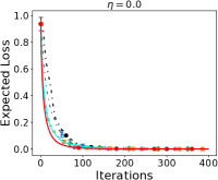
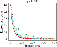
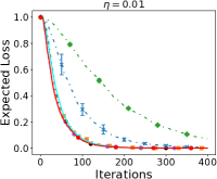
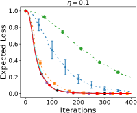
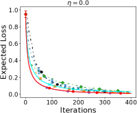
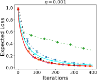
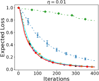
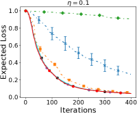
Figure 3: Result of $\max_{p\in{\cal P}}\mathbb{E}_{p(\boldsymbol{x}^{*})}\left[\sigma_{t}^{2}(\boldsymbol{x}^{*})\right]$ in the synthetic data experiments with $\eta=0,0.001,0.01,0.1$. The horizontal and vertical axes show the number of iterations and $\max_{p\in{\cal P}}\mathbb{E}_{p(\boldsymbol{x}^{*})}\left[\sigma_{t}^{2}(\boldsymbol{x}^{*})\right]$, respectively. The error bar shows mean and standard errors for 20 random trials regarding the random initial point (and the algorithm’s randomness). The top and bottom columns represent the results of the GPR model with SE and Matérn kernels, respectively.

C.2 Details on Implementation of EPIG

EPIG is defined as follows [Bickford Smith et al., 2023]:

$$\boldsymbol{x}_{t}=\operatorname*{arg\,max}_{\boldsymbol{x}\in{\cal X}}\mathbb{E}_{p(\boldsymbol{x}^{*})}\left[H[y_{\boldsymbol{x}^{*}}\mid{\cal D}_{t-1},\boldsymbol{x}]-H[y_{\boldsymbol{x}^{*}}\mid{\cal D}_{t-1}]\right].$$

Although Bickford Smith et al. [2023] have discussed the efficient computation for EPIG, in the regression problem, the EPIG can be computed analytically except for the expectation over $p(\boldsymbol{x}^{*})$ as follows:

$$\boldsymbol{x}_{t}=\operatorname*{arg\,max}_{\boldsymbol{x}\in{\cal X}}\mathbb{E}_{p(\boldsymbol{x}^{*})}\left[\log\left(\frac{\sigma_{t-1}^{2}(\boldsymbol{x},\boldsymbol{x}^{*})}{\sqrt{\sigma_{t-1}^{2}(\boldsymbol{x})+\sigma^{2}}\sqrt{\sigma_{t-1}^{2}(\boldsymbol{x}^{*})+\sigma^{2}}}\right)\right],$$

where $\sigma_{t-1}^{2}(\boldsymbol{x},\boldsymbol{x}^{*})$ is the posterior covariance between $\boldsymbol{x}$ and $\boldsymbol{x}^{*}$. Since we focus on the discrete input domain in the experiments, the expectation over $p(\boldsymbol{x}^{*})$ can also be computed analytically. We used the above equation for the implementation.

C.3 Details on Real-World Datasets

The King County house sales dataset is a dataset used to predict house prices in King County by 7-dimensional features, such as the area and the number of rooms. This dataset has been used for testing the regression [Park et al., 2020], and a similar dataset has also been used for the AL studies [Park and Kim, 2020]. Although this dataset includes 20000 data, we used randomly chosen 1000 data for simplicity.

Red wine quality dataset [Cortez and Reis, 2009] is a dataset used to predict the quality of wines from the wine ingredients expressed by 11-dimensional features. This dataset includes 1600 data and has been used for the regression problem [Cortez et al., 2009].

Auto MPG dataset [Quinlan, 1993] is a dataset used to predict automobile fuel efficiency from 6-dimensional features, such as the weight of the automobile and engine horsepower. Auto MPG dataset has been used for the AL reserch [Park and Kim, 2020]. This dataset includes 399 data.

References

- Abbasi-Yadkori (2013) Yasin Abbasi-Yadkori. Online learning for linearly parametrized control problems. PhD thesis, University of Alberta, 2013.
- Adler (1981) Robert J Adler. The Geometry of Random Fields, volume 62. SIAM, 1981.
- Agrawal et al. (2018) Akshay Agrawal, Robin Verschueren, Steven Diamond, and Stephen Boyd. A rewriting system for convex optimization problems. Journal of Control and Decision, 5(1):42–60, 2018.
- Allen-Zhu et al. (2017) Zeyuan Allen-Zhu, Yuanzhi Li, Aarti Singh, and Yining Wang. Near-optimal design of experiments via regret minimization. In Proceedings of the 34th International Conference on Machine Learning, volume 70 of Proceedings of Machine Learning Research, pages 126–135. PMLR, 2017.
- Bian et al. (2017) Andrew An Bian, Joachim M. Buhmann, Andreas Krause, and Sebastian Tschiatschek. Guarantees for greedy maximization of non-submodular functions with applications. In Proceedings of the 34th International Conference on Machine Learning, volume 70 of Proceedings of Machine Learning Research, pages 498–507. PMLR, 2017.
- Bickford Smith et al. (2023) Freddie Bickford Smith, Andreas Kirsch, Sebastian Farquhar, Yarin Gal, Adam Foster, and Tom Rainforth. Prediction-oriented Bayesian active learning. In Proceedings of The 26th International Conference on Artificial Intelligence and Statistics, volume 206 of Proceedings of Machine Learning Research, pages 7331–7348. PMLR, 2023.
- Bogunovic et al. (2016) Ilija Bogunovic, Jonathan Scarlett, Andreas Krause, and Volkan Cevher. Truncated variance reduction: A unified approach to Bayesian optimization and level-set estimation. In Advances in neural information processing systems 29, pages 1507–1515. Curran Associates, Inc., 2016.
- Chaloner and Verdinelli (1995) Kathryn Chaloner and Isabella Verdinelli. Bayesian Experimental Design: A Review. Statistical Science, 10(3):273 – 304, 1995.
- Chen and Paschalidis (2018) Ruidi Chen and Ioannis Ch. Paschalidis. A robust learning approach for regression models based on distributionally robust optimization. Journal of Machine Learning Research, 19(13):1–48, 2018.
- Chen et al. (2020) Ruidi Chen, Ioannis Ch Paschalidis, et al. Distributionally robust learning. Foundations and Trends® in Optimization, 4(1-2):1–243, 2020.
- Chowdhury and Gopalan (2017) Sayak Ray Chowdhury and Aditya Gopalan. On kernelized multi-armed bandits. In Proceedings of the 34th International Conference on Machine Learning, volume 70 of Proceedings of Machine Learning Research, pages 844–853, 2017.
- Cohn (1993) David Cohn. Neural network exploration using optimal experiment design. Advances in neural information processing systems, 6, 1993.
- Cohn et al. (1996) David A Cohn, Zoubin Ghahramani, and Michael I Jordan. Active learning with statistical models. Journal of artificial intelligence research, 4:129–145, 1996.
- Cortez and Reis (2009) Cerdeira A. Almeida F. Matos T. Cortez, Paulo and J. Reis. Wine Quality. UCI Machine Learning Repository, 2009.
- Cortez et al. (2009) Paulo Cortez, Juliana Teixeira, António Cerdeira, Fernando Almeida, Telmo Matos, and José Reis. Using data mining for wine quality assessment. In Discovery Science: 12th International Conference, pages 66–79. Springer, 2009.
- Costa et al. (2024) Nathaël Da Costa, Marvin Pförtner, Lancelot Da Costa, and Philipp Hennig. Sample path regularity of Gaussian processes from the covariance kernel, 2024.
- Das and Kempe (2008) Abhimanyu Das and David Kempe. Algorithms for subset selection in linear regression. In Proceedings of the Fortieth Annual ACM Symposium on Theory of Computing, STOC ’08, page 45â54. Association for Computing Machinery, 2008.
- De Freitas et al. (2012) Nando De Freitas, Alex J. Smola, and Masrour Zoghi. Exponential regret bounds for Gaussian process bandits with deterministic observations. In Proceedings of the 29th International Conference on International Conference on Machine Learning, page 955â962. Omnipress, 2012.
- Diamond and Boyd (2016) Steven Diamond and Stephen Boyd. CVXPY: A Python-embedded modeling language for convex optimization. Journal of Machine Learning Research, 17(83):1–5, 2016.
- Frogner et al. (2021) Charlie Frogner, Sebastian Claici, Edward Chien, and Justin Solomon. Incorporating unlabeled data into distributionally robust learning. Journal of Machine Learning Research, 22(56):1–46, 2021.
- Ghosal and Roy (2006) Subhashis Ghosal and Anindya Roy. Posterior consistency of Gaussian process prior for nonparametric binary regression. The Annals of Statistics, 34(5):2413 – 2429, 2006.
- Gotovos et al. (2013) Alkis Gotovos, Nathalie Casati, Gregory Hitz, and Andreas Krause. Active learning for level set estimation. In Proceedings of the Twenty-Third international joint conference on Artificial Intelligence, pages 1344–1350, 2013.
- Guestrin et al. (2005) Carlos Guestrin, Andreas Krause, and Ajit Paul Singh. Near-optimal sensor placements in Gaussian processes. In Proceedings of the 22nd International Conference on Machine Learning, page 265â272. Association for Computing Machinery, 2005.
- Handel (2016) Ramon Van Handel. Probability in high dimension, 2016. Lecture notes. Available in https://web.math.princeton.edu/˜rvan/APC550.pdf.
- Hanneke et al. (2014) Steve Hanneke et al. Theory of disagreement-based active learning. Foundations and Trends® in Machine Learning, 7(2-3):131–309, 2014.
- Hoang et al. (2014) Trong Nghia Hoang, Bryan Kian Hsiang Low, Patrick Jaillet, and Mohan Kankanhalli. Nonmyopic -Bayes-optimal active learning of Gaussian processes. In International conference on machine learning, pages 739–747. PMLR, 2014.
- Houlsby et al. (2011) Neil Houlsby, Ferenc Huszár, Zoubin Ghahramani, and Máté Lengyel. Bayesian active learning for classification and preference learning. arXiv preprint arXiv:1112.5745, 2011.
- Hu and Hong (2013) Zhaolin Hu and L Jeff Hong. Kullback-leibler divergence constrained distributionally robust optimization. Available at Optimization Online, 1(2):9, 2013.
- Inatsu et al. (2021) Yu Inatsu, Shogo Iwazaki, and Ichiro Takeuchi. Active learning for distributionally robust level-set estimation. In Proceedings of the 38th International Conference on Machine Learning, volume 139 of Proceedings of Machine Learning Research, pages 4574–4584. PMLR, 2021.
- Inatsu et al. (2024) Yu Inatsu, Shion Takeno, Kentaro Kutsukake, and Ichiro Takeuchi. Active learning for level set estimation using randomized straddle algorithms. Transactions on Machine Learning Research, 2024.
- Kanagawa et al. (2018) Motonobu Kanagawa, Philipp Hennig, Dino Sejdinovic, and Bharath K Sriperumbudur. Gaussian processes and kernel methods: A review on connections and equivalences, 2018.
- Kandasamy et al. (2018) Kirthevasan Kandasamy, Akshay Krishnamurthy, Jeff Schneider, and Barnabas Póczos. Parallelised Bayesian optimisation via Thompson sampling. In Proceedings of the 21st International Conference on Artificial Intelligence and Statistics, volume 84 of Proceedings of Machine Learning Research, pages 133–142, 2018.
- Kirsch and Gal (2022) Andreas Kirsch and Yarin Gal. Unifying approaches in active learning and active sampling via Fisher information and information-theoretic quantities. Transactions on Machine Learning Research, 2022. Expert Certification.
- Kirsch et al. (2021) Andreas Kirsch, Tom Rainforth, and Yarin Gal. Test distribution-aware active learning: A principled approach against distribution shift and outliers, 2021.
- Kirschner and Krause (2018) Johannes Kirschner and Andreas Krause. Information directed sampling and bandits with heteroscedastic noise. In Proceedings of the 31st Conference On Learning Theory, volume 75 of Proceedings of Machine Learning Research, pages 358–384. PMLR, 2018.
- Krause et al. (2008a) Andreas Krause, H. Brendan McMahan, Carlos Guestrin, and Anupam Gupta. Robust submodular observation selection. Journal of Machine Learning Research, 9(93):2761–2801, 2008a.
- Krause et al. (2008b) Andreas Krause, Ajit Singh, and Carlos Guestrin. Near-optimal sensor placements in Gaussian processes: Theory, efficient algorithms and empirical studies. J. Mach. Learn. Res., 9:235â284, 2008b.
- Kusakawa et al. (2022) Shunya Kusakawa, Shion Takeno, Yu Inatsu, Kentaro Kutsukake, Shogo Iwazaki, Takashi Nakano, Toru Ujihara, Masayuki Karasuyama, and Ichiro Takeuchi. Bayesian optimization for cascade-type multistage processes. Neural Computation, 34(12):2408–2431, 2022.
- Kushner (1964) H. J. Kushner. A New Method of Locating the Maximum Point of an Arbitrary Multipeak Curve in the Presence of Noise. Journal of Basic Engineering, 86(1):97–106, 1964.
- Li and Scarlett (2022) Zihan Li and Jonathan Scarlett. Gaussian process bandit optimization with few batches. In Proceedings of The 25th International Conference on Artificial Intelligence and Statistics, volume 151 of Proceedings of Machine Learning Research, pages 92–107. PMLR, 2022.
- Lindley (1956) D. V. Lindley. On a Measure of the Information Provided by an Experiment. The Annals of Mathematical Statistics, 27(4):986 – 1005, 1956.
- Paria et al. (2020) Biswajit Paria, Kirthevasan Kandasamy, and Barnabás Póczos. A flexible framework for multi-objective Bayesian optimization using random scalarizations. In Proceedings of The 35th Uncertainty in Artificial Intelligence Conference, volume 115 of Proceedings of Machine Learning Research, pages 766–776, 2020.
- Park et al. (2020) Minyoung Park, Seungyeon Lee, Sangheum Hwang, and Dohyun Kim. Additive ensemble neural networks. IEEE Access, 8:113192–113199, 2020.
- Park and Kim (2020) Sung Ho Park and Seoung Bum Kim. Robust expected model change for active learning in regression. Applied Intelligence, 50:296–313, 2020.
- Pukelsheim (2006) Friedrich Pukelsheim. Optimal design of experiments. SIAM, 2006.
- Quinlan (1993) R. Quinlan. Auto MPG. UCI Machine Learning Repository, 1993. DOI: https://doi.org/10.24432/C5859H.
- Rasmussen and Williams (2005) Carl Edward Rasmussen and Christopher K. I. Williams. Gaussian Processes for Machine Learning (Adaptive Computation and Machine Learning). The MIT Press, 2005.
- Ryan and Morgan (2007) Thomas P Ryan and JP Morgan. Modern experimental design. Journal of Statistical Theory and Practice, 1(3-4):501–506, 2007.
- Salgia et al. (2024) Sudeep Salgia, Sattar Vakili, and Qing Zhao. Random exploration in Bayesian optimization: Order-optimal regret and computational efficiency. In Proceedings of the 41st International Conference on Machine Learning, volume 235 of Proceedings of Machine Learning Research, pages 43112–43141. PMLR, 2024.
- Sener and Savarese (2018) Ozan Sener and Silvio Savarese. Active learning for convolutional neural networks: A core-set approach. In International Conference on Learning Representations, 2018.
- Seo et al. (2000) Sambu Seo, M. Wallat, T. Graepel, and K. Obermayer. Gaussian process regression: active data selection and test point rejection. In Proceedings of the IEEE-INNS-ENNS International Joint Conference on Neural Networks. IJCNN 2000. Neural Computing: New Challenges and Perspectives for the New Millennium, volume 3, pages 241–246, 2000.
- Settles (2009) Burr Settles. Active learning literature survey. Computer Sciences Technical Report 1648, University of Wisconsin–Madison, 2009.
- Shahriari et al. (2016) Bobak Shahriari, Kevin Swersky, Ziyu Wang, Ryan P. Adams, and Nando De Freitas. Taking the human out of the loop: A review of Bayesian optimization. Proceedings of the IEEE, 104(1):148–175, 2016.
- Shoham and Avron (2023) Neta Shoham and Haim Avron. Experimental Design for Overparameterized Learning With Application to Single Shot Deep Active Learning . IEEE Transactions on Pattern Analysis & Machine Intelligence, 45(10):11766–11777, 2023.
- Srinivas et al. (2010) N. Srinivas, A. Krause, S. Kakade, and M. Seeger. Gaussian process optimization in the bandit setting: No regret and experimental design. In Proceedings of the 27th International Conference on Machine Learning, pages 1015–1022. Omnipress, 2010.
- Staib et al. (2019) Matthew Staib, Bryan Wilder, and Stefanie Jegelka. Distributionally robust submodular maximization. In Proceedings of the Twenty-Second International Conference on Artificial Intelligence and Statistics, volume 89 of Proceedings of Machine Learning Research, pages 506–516. PMLR, 2019.
- Sugiyama (2005) Masashi Sugiyama. Active learning for misspecified models. In Advances in Neural Information Processing Systems, volume 18, pages 1305–1312. MIT Press, 2005.
- Takeno et al. (2023) Shion Takeno, Yu Inatsu, and Masayuki Karasuyama. Randomized Gaussian process upper confidence bound with tighter Bayesian regret bounds. In Proceedings of the 40th International Conference on Machine Learning, volume 202 of Proceedings of Machine Learning Research, pages 33490–33515. PMLR, 2023.
- Takeno et al. (2024) Shion Takeno, Yu Inatsu, Masayuki Karasuyama, and Ichiro Takeuchi. Posterior sampling-based Bayesian optimization with tighter Bayesian regret bounds. In Proceedings of the 41st International Conference on Machine Learning, volume 235 of Proceedings of Machine Learning Research, pages 47510–47534. PMLR, 2024.
- Vakili et al. (2021a) Sattar Vakili, Nacime Bouziani, Sepehr Jalali, Alberto Bernacchia, and Da-shan Shiu. Optimal order simple regret for Gaussian process bandits. In Advances in Neural Information Processing Systems, volume 34, pages 21202–21215. Curran Associates, Inc., 2021a.
- Vakili et al. (2021b) Sattar Vakili, Kia Khezeli, and Victor Picheny. On information gain and regret bounds in Gaussian process bandits. In Proceedings of The 24th International Conference on Artificial Intelligence and Statistics, volume 130 of Proceedings of Machine Learning Research, pages 82–90, 2021b.
- Vakili et al. (2022) Sattar Vakili, Jonathan Scarlett, Da-shan Shiu, and Alberto Bernacchia. Improved convergence rates for sparse approximation methods in kernel-based learning. In International Conference on Machine Learning, pages 21960–21983. PMLR, 2022.
- van der Vaart and Wellner (1996) Aad van der Vaart and Jon A Wellner. Weak Convergence and Empirical Processes: With Applications to Statistics. Springer Science & Business Media, 1996.
- Yu et al. (2006) Kai Yu, Jinbo Bi, and Volker Tresp. Active learning via transductive experimental design. In Proceedings of the 23rd international conference on Machine learning, pages 1081–1088, 2006.
- Zhao et al. (2021) Eric Zhao, Anqi Liu, Animashree Anandkumar, and Yisong Yue. Active learning under label shift. In International conference on artificial intelligence and statistics, pages 3412–3420. PMLR, 2021.