Joint Size and Placement Optimization for IRS-Aided Communications with Active and Passive Elements

Abstract

Different types of intelligent reflecting surfaces (IRS) are exploited for assisting wireless communications. The joint use of passive IRS (PIRS) and active IRS (AIRS) emerges as a promising solution owing to their complementary advantages. They can be integrated into a single hybrid active-passive IRS (HIRS) or deployed in a distributed manner, which poses challenges in determining the IRS elements allocation and placement for rate maximization. In this paper, we investigate the capacity of an IRS-aided wireless communication system with both active and passive elements. Specifically, we consider three deployment schemes: 1) base station (BS)→HIRS→user (BHU); 2) BS→AIRS→PIRS→user (BAPU); 3) BS→PIRS→AIRS→user (BPAU). Under the line-of-sight channel model, we formulate a rate maximization problem via a joint optimization of the IRS elements allocation and placement. We first derive the optimized number of active and passive elements for BHU, BAPU, and BPAU schemes, respectively. Then, low-complexity HIRS/AIRS placement strategies are provided. To obtain more insights, we characterize the system capacity scaling orders for the three schemes with respect to the large total number of IRS elements, amplification power budget, and BS transmit power. Finally, simulation results are presented to validate our theoretical findings and show the performance difference among the BHU, BAPU, and BPAU schemes with the proposed joint design under various system setups.

I Introduction

Intelligent reflecting surface (IRS) has gained significant attention in facilitating the widespread application of wireless networks due to its energy and cost efficiency as well as flexible deployment [1, 2, 3, 4, 5]. Specifically, passive IRS (PIRS) can construct an intelligent wireless propagation environment by smartly adjusting the phase shift of each reflecting element [6, 7, 8, 9, 10, 11]. However, it suffers from severe product-distance path loss in practice. To overcome this challenge, active IRS (AIRS) has been proposed to enhance the reflected signal power thanks to its amplification capabilities, whereas it introduces negligible amplification noise [12, 13, 14, 15].

Recently, extensive works have explored integrating AIRS and PIRS into a single system to leverage their complementary advantages. One of the effective ways is co-locating both active and passive elements to form a single large IRS, which is known as a hybrid active-passive IRS (HIRS) [16, 17, 18, 19, 20, 21, 22, 23, 24]. Specifically, [18] proposed alternating optimization (AO) based optimization algorithms for energy efficiency maximization in an HIRS-assisted downlink communication. The joint beamforming design was investigated in [19, 20] for different systems, i.e., secure communication and millimeter-wave integrated sensing and communication systems, respectively. Benefiting from flexibly balancing the amplification gain and beamforming gain, the results in [16, 17, 18, 19, 20] demonstrated that the HIRS can outperform both AIRS and PIRS in most practical scenarios. In contrast, another design integrating AIRS and PIRS is deploying distributed AIRS and PIRS by grouping reflecting elements of the same type on two or more small IRS. Despite a higher power scaling order provided by the systems with two or more PIRSs thanks to the benefits of double or multiple reflections, multiplicative fading and beam routing remains critical issues in these systems [25, 26, 27, 28, 29, 30, 31, 32]. The AIRSs can be deployed to achieve signal amplification [33, 34, 35], whereas it involves more complex design considerations. This is because they require the joint optimization of both the reflection amplitude and phase of the active elements. In addition, a new design trade-off emerges between the received signal power maximization and the noise amplification power minimization. By taking advantage of AIRS and PIRS, [36, 37] studied the achievable rate maximization problem in two distributed AIRS and PIRS jointly aided communication systems, i.e., base station (BS)→AIRS→PIRS→user (BAPU) and BS→PIRS→AIRS→user (BPAU).

PIRS can achieve a higher beamforming gain when the number of reflecting elements is large, whereas AIRS can offer unique power amplification gain, resulting in significantly higher SNR with fewer reflecting elements [16]. To fully reap the potential advantages of double IRS or HIRS to balance the trade-off between the amplification and beamforming gains, it is crucial to carefully design its elements allocation [38, 16, 17, 39, 37]. For example, [38] considered the scenario where two distributed PIRSs are respectively equipped with $N/2$ passive elements, which yields a power scaling order of $\mathcal{O}(N^{4})$. For a communication system with the BHU scheme, i.e., BS→HIRS→user, [16] focused on the ergodic capacity maximization, while considering constraints such as the total deployment and amplification power budget. [17] further studied the impact of the number of active and passive elements at the HIRS on the system energy efficiency maximization. Moreover, the authors in [39] studied the HIRS elements allocation for minimizing the latency and energy consumption in a mobile edge computing system. With the joint use of AIRS and PIRS, [37] showed that the optimal number of passive elements should be twice that of active elements to maximize the achievable rate under two different deployment orders with a given deployment budget.

To fully exploit the superior flexibility and compatibility of the IRS for practical implementation, the IRS placement should be investigated in addition to its elements allocation design. The objective of optimizing IRS deployment is to enable the reflected signal to bypass obstacles, ensuring signal coverage and maximizing the received signal power, thereby further improving system performance [40, 41, 42, 43, 44, 36, 31, 45, 46]. The results in [40] demonstrated that the PIRS should be placed close to the BS or user to minimize the double path loss effect for a single-user setup. A double PIRS placement optimization problem was solved to mitigate inter-cell interference in air-ground communication networks in [41]. The work was further extended to a multiple PIRS-aided multi-user communication system for the minimum achievable rate maximization in [42]. It was revealed in [43, 44] that the placement strategy of an AIRS is different from that of a PIRS to strike a balance between signal and noise amplification. In [43], the impact of the amplification power on the optimal location of AIRS was characterized, which showed that the amplification noise can be compensated by deploying the AIRS closer to the receiver. Moreover, [36] focused on the AIRS deployment design under BAPU and BPAU schemes. To summarize, the performance of the IRS-aided system with both active and passive elements is sensitive to the IRS location.

All the above works focus only on either IRS elements allocation or placement, but they affect each other. As such, it requires joint design, which takes into account the interaction between the two key factors. Under a more comprehensive consideration of system requirements, the joint elements allocation and placement design can be exploited to find a better strategy to improve system performance. Due to the above benefits, the authors in [47, 48, 49] aimed to further improve the system’s performance by jointly optimizing the IRS elements allocation and placement. For example, the authors of [47] studied the minimum outage probability with the joint design of the PIRS location and size optimization under various constraints. For a double AIRS-aided communication system, an efficient algorithm was proposed in [48] to solve the minimum rate maximization problem involving combinatorial optimization with a fixed per-element amplification power. For a single-user setup, [49] derived the optimal solution in closed form for maximizing the achievable rate and obtained more insights under the total amplification power constraint. Regarding a system where both active and passive elements are deployed, several issues remain to be resolved. First, how to design the joint optimization of IRS elements allocation and placement? For BAPU and BPAU schemes, it can lead to performance degradation or even complete failure of the entire link if the performance of one of the IRSs is limited. This is due to the fact that signal transmission needs to pass through both AIRS and PIRS under both schemes. In contrast, the other type can compensate for the failure if one type of reflecting element at the HIRS fails, ensuring the signal transmission despite performance loss, which shows the robustness and flexibility of BHU. Given the different deployment strategies of AIRS and PIRS, it still remains unknown how to design the HIRS deployment for further improving the system rate performance. Second, do BAPU and BPAU always outperform BHU? This question arises from the cases of double AIRS and double PIRS compared to their single counterparts. BAPU and BPAU schemes may reap greater beamforming gains through cooperation because the double reflection of the signal results in higher signal power being received at the user and extends the coverage.

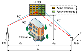
(a) BHU scheme

(b) BAPU scheme

(c) BPAU scheme

Figure 1: Illustration of the considered systems.

Motivated by the above, we focus on characterizing the capacity of the joint active and passive IRS-aided wireless system. We aim to establish an analytical framework that enables a theoretical comparison of the capacity among three different deployment schemes, namely, BHU, BAPU, and BPAU (See Fig. 1). The capacity characterization problem involves the joint design of the IRS beamforming, elements allocation, and placement, which renders it more challenging than the previous work. The main contributions of this paper are summarized as follows.

• First, we study a wireless communication system by comparing BHU, BAPU, and BPAU schemes. For the BHU scheme, a single-reflection link is provided via the HIRS, while both the BAPU and BPAU schemes establish a double-reflection link using two IRSs between the BS and the user. Based on the proposed models, the corresponding achievable rate maximization problems are formulated by jointly optimizing the active and passive elements allocation and IRS location.

• Second, we derive the optimal number of active and passive elements for the three schemes. To obtain useful insights, we propose low-complexity solutions for BAPU and BPAU schemes in closed form with the given assumptions. Our analytic results show that more passive elements should be deployed at the PIRS for both BAPU and BPAU schemes as the total number of IRS elements $N$ increases. However, for the BHU scheme, the number of passive elements first remains at one and then linearly increases with respect to (w.r.t.) $N$ after it exceeds a threshold. Moreover, the BHU scheme is preferable when deploying the HIRS close to the user and the BAPU (BPAU) scheme performs best when the PIRS is close to the user (BS), which motivates us to further design the IRS placement.

• Based on the closed-form expressions of the IRS placement, we characterize the impact of key system parameters on the optimized horizontal BS-HIRS/AIRS distance. It reveals that the corresponding distance monotonically increases with the BS transmit power and decreases with the amplification power budget under the three schemes. Moreover, the results suggest that BPAU and BPAU should be avoided when the amplification power budget or transmit power is small, respectively.

• To obtain more insights, we theoretically analyze the asymptotic SNR and then characterize the capacity scaling orders for the three schemes w.r.t. the total number of reflecting elements, transmit power, and amplification power, which lay the foundation for performance comparison. The results show that the BHU scheme outperforms both BAPU and BPAU schemes with a sufficient total number of IRS elements or transmit power, whereas the latter two schemes perform better when a large amplification power is affordable.

• Finally, numerical results demonstrate that BHU is an energy-efficient solution for maximizing the capacity, especially in space-limited scenarios. In contrast, BAPU can achieve better rate performance when the transmit power budget is sufficiently large, whereas BPAU is preferable when the total number of IRS reflecting elements is large. Moreover, the results demonstrate that the joint active and passive IRS-aided wireless system with our proposed design can reap considerable performance gains over other benchmark systems.

The rest of this paper is organized as follows. Section II describes our system model and problem formulations considering BHU, BAPU, and BPAU schemes. Section III addresses the IRS elements allocation and placement problem. In Section IV, we analytically characterize the system capacity scaling orders. Section V presents simulation results to validate our theoretical analysis and provide further numerical comparison among the three schemes. Finally, we conclude in Section VI.

Notations: $\mathbb{N}^{{}^{+}}$ denotes the the set of positive natural numbers. For a complex-valued vector $\mathbf{x}$, ${\left[\mathbf{x}\right]}_{m}$ denotes the $m$-th entry of $\mathbf{x}$, $\arg\left(\mathbf{x}\right)$ represents its phase, and $\operatorname{diag}\left(\mathbf{x}\right)$ denotes a diagonal matrix with the elements in $\mathbf{x}$ on its main diagonal. $\mathbf{I}_{n}$ is an identity matrix of dimensions $n\times n$. $\left(\cdot\right)^{H}$, $\frac{{\partial}}{{\partial}}\left(\cdot\right)$, and $\|\cdot\|$ stand for conjugate transpose operators, the partial derivative, and Euclidean norm, respectively. $\mathcal{CN}(\mu,\sigma^{2})$ denotes the circularly symmetric complex Gaussian distribution with a mean of $\mu$ and variance of $\sigma^{2}$. $\mathcal{O}\left(\cdot\right)$ represents the big-O notation. $\otimes$ denotes the Kronecker product.

II System Model and Problem Formulations

As illustrated in Fig. 1, we consider an IRS-aided wireless system, where the IRS with $N_{\mathrm{p}}$ passive elements and $N_{\mathrm{a}}$ active elements are deployed to enhance the transmission from a single-antenna BS to a single-antenna user in a given zone. The direct BS-user, BS-IRS 2, and IRS 1-user links are assumed to be blocked due to dense obstacles, and the line-of-sight (LoS) channel model is used for other available links. According to [52], we assume that the channel state information of the considered links is available. Three different deployment schemes are considered, namely, BHU, BAPU, and BPAU. Specifically, a total of $N=N_{\mathrm{p}}+N_{\mathrm{a}}$ IRS elements form one single HIRS for the BHU scheme, which is deployed in the LoS region of the BS and the user (see Fig. 1 (a)). By contrast, passive and active elements are deployed at two distributed IRS for BAPU and BPAU schemes, where IRS 1 and IRS 2 are located in the vicinity of the BS and the user, respectively (see Fig. 1 (b) and (c)). Under a three-dimensional Cartesian coordinate system, the BS, the HIRS, IRS 1, IRS 2, and the user are located at $\bm{u}_{\mathrm{B}}=(0,0,0)$ and $\bm{u}_{0}=(x_{\mathrm{BI}},0,h_{\mathrm{s}})$, $\bm{u}_{1}=(x_{\mathrm{B}},0,h_{\mathrm{d}})$, $\bm{u}_{2}=(L-x_{\mathrm{U}},0,h_{\mathrm{d}})$, and $\bm{u}_{\mathrm{u}}=(L,0,0)$, respectively. As such, the distances between the BS and HIRS, the HIRS and user, the BS and IRS 1, the IRS 1 and IRS 2, and the IRS 2 and user are given by $d_{\mathrm{BI}}=\sqrt{x_{\mathrm{BI}}^{2}+h_{\mathrm{s}}^{2}}$, $d_{\mathrm{IU}}=\sqrt{x_{\mathrm{IU}}^{2}+h_{\mathrm{s}}^{2}}$, $d_{\mathrm{B}}=\sqrt{x_{\mathrm{B}}^{2}+h_{\mathrm{d}}^{2}}$, $d_{\mathrm{I}}=L-x_{\mathrm{B}}-x_{\mathrm{U}}$, and $d_{\mathrm{U}}=\sqrt{x_{\mathrm{U}}^{2}+h_{\mathrm{d}}^{2}}$, respectively.

Let $\mathcal{N}_{\mathrm{p}}$ and $\mathcal{N}_{\mathrm{a}}$ denote the sets of all elements on the PIRS and AIRS, respectively. The reflection matrices of PIRS/passive IRS sub-surface and AIRS/active IRS sub-surface are denoted by ${\mathbf{\Psi}}_{{\mathrm{p}}}=\operatorname{diag}(e^{j\phi_{{\mathrm{p}},1}},\ldots,e^{j\phi_{{\mathrm{p}},N_{\mathrm{p}}}})$ and ${\mathbf{\Psi}}_{\mathrm{a}}={\mathbf{A}}_{{\mathrm{a}}}\mathbf{\Phi}_{\mathrm{a}}$, respectively, where ${\mathbf{A}}_{{\mathrm{a}}}=\operatorname{diag}(\alpha_{\mathrm{a},1},\ldots,\alpha_{\mathrm{a},N_{\mathrm{a}}})$ and ${\mathbf{\Phi}}_{{\mathrm{a}}}=\operatorname{diag}(e^{j\phi_{{\mathrm{a}},1}},\ldots,e^{j\phi_{{\mathrm{a}},N_{\mathrm{a}}}})$ respectively denote the amplification matrix and phase-shift matrix. $\phi_{{\mathrm{p}},n},\forall n\in\mathcal{N}_{\mathrm{p}}(\phi_{{\mathrm{a}},n},\forall n\in\mathcal{N}_{\mathrm{a}})$ and $\alpha_{\mathrm{a},n},\forall n\in\mathcal{N}_{\mathrm{a}}$ represent the passive (active) phase shift and the active amplification factor at element $n$, respectively. We define the receive response vector as $\mathbf{a}_{\mathrm{r}}(\theta^{\mathrm{r}}_{i,k},\vartheta^{\mathrm{r}}_{i,k},N_{\mathrm{p}})=\bm{w}(\frac{2\Delta_{\mathrm{d}}}{\lambda}\sin(\theta^{\mathrm{r}}_{i,k})\sin(\vartheta^{\mathrm{r}}_{i,k}),N_{k,x})\otimes\bm{w}(\frac{2\Delta_{\mathrm{d}}}{\lambda}\cos(\vartheta^{\mathrm{r}}_{i,k}),N_{k,y})$, where $\lambda$ denotes the signal wavelength, $\Delta_{\mathrm{d}}$ represents the reflecting element space, $\theta^{\mathrm{r}}_{i,k}(\vartheta^{\mathrm{r}}_{i,k})$ is the azimuth (elevation) angle-of-arrival at node $k$ from node $i$, $N_{k,x}(N_{k,y})$ denotes the number of horizon (vertical) elements at node $k$ with $N_{k}=N_{k,x}\times N_{k,y}$, and $\bm{w}(\theta,N^{\prime})=[1,\ldots,e^{-j\pi(N^{\prime}-1)\theta}]^{T}$ denotes the steering vector function. The transmit steering vector $\mathbf{a}_{\mathrm{t}}$ can be defined similarly as $\mathbf{a}_{\mathrm{r}}$. Next, the system models for the considered schemes are described in detail.

II-A BHU Scheme

For BHU scheme, the channel from BS to the passive IRS sub-surface and that from the passive IRS sub-surface to the user are denoted by $\mathbf{h}^{\mathrm{p}}_{\mathrm{BI}}=\beta_{\mathrm{BI}}\mathbf{a}_{\mathrm{r}}(\theta^{\mathrm{r}}_{\mathrm{BS},\mathrm{H}},\vartheta^{\mathrm{r}}_{\mathrm{BS},\mathrm{H}},N_{\mathrm{p}})$ and $\mathbf{h}^{\mathrm{p}}_{\mathrm{IU}}=\beta_{\mathrm{IU}}\mathbf{a}_{\mathrm{t}}(\theta^{\mathrm{t}}_{\mathrm{H},\mathrm{U}},\vartheta^{\mathrm{t}}_{\mathrm{H},\mathrm{U}},N_{\mathrm{p}})$, respectively, where $\beta_{\mathrm{BI}}$ and $\beta_{\mathrm{IU}}$ denote the corresponding complex-valued path gains. The channel from BS to active IRS sub-surface $\mathbf{h}^{\mathrm{a}}_{\mathrm{BI}}$ and the channel from active IRS sub-surface to the user $\mathbf{h}^{\mathrm{a}}_{\mathrm{IU}}$ can be modeled similarly to $\mathbf{h}^{\mathrm{p}}_{\mathrm{BI}}$ and $\mathbf{h}^{\mathrm{p}}_{\mathrm{IU}}$. Let $P_{\mathrm{I}}$ denote the amplification power budget of the active elements and then we have

$${P_{\mathrm{B}}}{\left\|{{{\mathbf{\Psi}}_{{\mathrm{a}}}}{\mathbf{h}}_{{\mathrm{BI}}}^{{\mathrm{a}}}}\right\|^{2}}+\sigma_{\mathrm{r}}^{2}{\left\|{{{\mathbf{\Psi}}_{{\mathrm{a}}}}{{\mathbf{I}}_{{N_{{\mathrm{a}}}}}}}\right\|^{2}}\leq{P_{\mathrm{I}}},$$ (1)

where $\sigma_{\mathrm{r}}^{2}$ denotes the amplification noise power. Though the single-reflection link, the signal received at the user is given by ${y_{\mathrm{0}}}={\left({{\mathbf{h}}_{{\mathrm{IU}}}^{{\mathrm{a}}}}\right)^{H}}{{\mathbf{\Psi}}_{{\mathrm{a}}}}{\mathbf{h}}_{{\mathrm{BI}}}^{{\mathrm{a}}}s+{\left({{\mathbf{h}}_{{\mathrm{IU}}}^{{\mathrm{p}}}}\right)^{H}}{{\mathbf{\Psi}}_{{\mathrm{p}}}}{\mathbf{h}}_{{\mathrm{BI}}}^{{\mathrm{p}}}s+{\left({{\mathbf{h}}_{{\mathrm{IU}}}^{{\mathrm{a}}}}\right)^{H}}{{\mathbf{\Psi}}_{{\mathrm{a}}}}{{\mathbf{n}}_{\mathrm{r}}}+{n_{0}}$, where $s\in\mathbb{C}$ represents the transmitted signal satisfying $\mathbb{E}\{{{{\left|s\right|}^{2}}}\}=P_{\mathrm{B}}$ with the BS transmit power $P_{\mathrm{B}}$, ${\mathbf{n}}_{\mathrm{r}}\sim\mathcal{CN}(\mathbf{0}_{N_{\mathrm{a}}},\sigma_{\mathrm{r}}^{2}\mathbf{I}_{N_{\mathrm{a}}})$ denotes the amplification noise introduced by active elements, and $n_{0}\sim\mathcal{CN}(0,\sigma_{0}^{2})$ denotes the additive white Gaussian noise (AWGN) at the user. Accordingly, the SNR at the user is given by

$${\gamma_{\mathrm{0}}}=\frac{{{P_{\mathrm{B}}}{{\left|{{{\left({{\mathbf{h}}_{{\mathrm{IU}}}^{{\mathrm{a}}}}\right)^{H}}}{{\mathbf{\Psi}}_{{\mathrm{a}}}}{\mathbf{h}}_{{\mathrm{BI}}}^{{\mathrm{a}}}+{{\left({{\mathbf{h}}_{{\mathrm{IU}}}^{{\mathrm{p}}}}\right)^{H}}}{{\mathbf{\Psi}}_{{\mathrm{p}}}}{\mathbf{h}}_{{\mathrm{BI}}}^{{\mathrm{p}}}}\right|}^{2}}}}{{\sigma_{\mathrm{r}}^{2}{{\left\|{{{\left({{\mathbf{h}}_{{\mathrm{IU}}}^{{\mathrm{a}}}}\right)^{H}}}{{\mathbf{\Psi}}_{{\mathrm{a}}}}}\right\|}^{2}}+\sigma_{0}^{2}}},$$ (2)

and the achievable rate for the BHU scheme is expressed as $R_{0}={{\log_{2}}\left({1+{\gamma_{\mathrm{0}}}}\right)}$. The phase of the HIRS should be designed to align in the BS-HIRS-user channels, i.e. ${{\left({{\mathbf{h}}_{{\mathrm{IU}}}^{{\mathrm{a}}}}\right)^{H}}}{{\mathbf{\Psi}}_{{\mathrm{a}}}}{\mathbf{h}}_{{\mathrm{BI}}}^{{\mathrm{a}}}$ and ${{\left({{\mathbf{h}}_{{\mathrm{IU}}}^{{\mathrm{p}}}}\right)^{H}}}{{\mathbf{\Psi}}_{{\mathrm{p}}}}{\mathbf{h}}_{{\mathrm{BI}}}^{{\mathrm{p}}}$. According to [16], the optimal HIRS beamforming can be expressed as $\phi_{{\mathrm{p}},n}=\arg\left({{{[{{\mathbf{h}}_{{\mathrm{IU}}}^{{\mathrm{p}}}}]_{n}}}}\right)-\arg\left({{{[{{\mathbf{h}}_{{\mathrm{BI}}}^{{\mathrm{p}}}}]_{n}}}}\right)$, $\phi_{{\mathrm{a}},n}=\arg\left({{{[{{\mathbf{h}}_{{\mathrm{IU}}}^{{\mathrm{a}}}}]_{n}}}}\right)-\arg\left({{{[{{\mathbf{h}}_{{\mathrm{BI}}}^{{\mathrm{a}}}}]_{n}}}}\right)$, and $\alpha_{\mathrm{a},n}={\alpha_{\mathrm{0}}}\triangleq\sqrt{{{{P_{\mathrm{I}}}}}/({{{N_{{\mathrm{a}}}}\left({{P_{\mathrm{B}}}\beta_{{\mathrm{BI}}}^{2}+\sigma_{\mathrm{r}}^{2}}\right)}})}$, which leads to

$${\gamma_{\mathrm{0}}}=\frac{{{P_{\mathrm{B}}}\beta_{{\mathrm{BI}}}^{2}\beta_{{\mathrm{IU}}}^{2}{{{\left({\sqrt{{N_{{\mathrm{a}}}}{P_{\mathrm{I}}}}+\sqrt{N_{{\mathrm{p}}}^{2}\left({{P_{\mathrm{B}}}\beta_{{\mathrm{BI}}}^{2}+\sigma_{\mathrm{r}}^{2}}\right)}}\right)^{2}}}}}}{{\sigma_{\mathrm{r}}^{2}{P_{\mathrm{I}}}\beta_{{\mathrm{IU}}}^{2}+\sigma_{0}^{2}{P_{\mathrm{B}}}\beta_{{\mathrm{BI}}}^{2}+\sigma_{0}^{2}\sigma_{\mathrm{r}}^{2}}}.$$ (3)

We aim to maximize the achievable rate by jointly optimizing the HIRS elements allocation $\mathbf{N}\buildrel\Delta\over{=}\left\{N_{\mathrm{p}},N_{\mathrm{a}}\right\}$ and placement $\mathbf{X}_{\mathrm{s}}\buildrel\Delta\over{=}\left\{x_{\mathrm{BI}},x_{\mathrm{IU}}\right\}$. The optimization problem is written as

$$\mathop{\max}\limits_{{\mathbf{N},\mathbf{X}_{\mathrm{s}}}}\;\;\; R_{0}$$ (4a)

$${\mathrm{s.t.}}\;\;\;\; N_{\mathrm{p}}+N_{\mathrm{a}}=N,$$ (4b)

$$N_{\mathrm{p}}\in\mathbb{N}^{+},N_{\mathrm{a}}\in\mathbb{N}^{+},$$ (4c)

$$x_{\mathrm{BI}}+x_{\mathrm{IU}}=L,$$ (4d)

$$x_{\mathrm{BI}}\geq 0,x_{\mathrm{IU}}\geq 0.$$ (4e)

II-B BAPU Scheme

For BAPU scheme, the channels from BS to the AIRS, from AIRS to PIRS, and from PIRS to user are denoted by $\mathbf{h}_{\mathrm{BA}}=\beta_{\mathrm{B}}\mathbf{a}_{\mathrm{r}}(\theta^{\mathrm{r}}_{\mathrm{BS},\mathrm{A}},\vartheta^{\mathrm{r}}_{\mathrm{BS},\mathrm{A}},N_{\mathrm{a}})$, ${{\mathbf{H}}_{{\mathrm{AP}}}}={\beta_{\mathrm{I}}}{{\mathbf{a}}_{\mathrm{r}}}\left({\theta_{{\mathrm{BS,A}}}^{\mathrm{r}},\vartheta_{{\mathrm{BS,A}}}^{\mathrm{r}},{N_{\mathrm{a}}}}\right){\mathbf{a}}_{\mathrm{t}}^{H}\left({\theta_{{\mathrm{P,U}}}^{\mathrm{r}},\vartheta_{{\mathrm{P,U}}}^{\mathrm{r}},{N_{\mathrm{p}}}}\right)$, and $\mathbf{h}_{\mathrm{PU}}=\beta_{\mathrm{U}}\mathbf{a}_{\mathrm{t}}(\theta^{\mathrm{t}}_{\mathrm{P},\mathrm{U}},\vartheta^{\mathrm{t}}_{\mathrm{P},\mathrm{U}},N_{\mathrm{p}})$, respectively, where $\beta_{\mathrm{B}}^{2}$, $\beta_{\mathrm{I}}^{2}$, and $\beta_{\mathrm{U}}^{2}$ denote the corresponding path loss. The amplification power constraint is given by

$${P_{\mathrm{B}}}{\left\|{{{\mathbf{\Psi}}_{{\mathrm{a}}}}{{\mathbf{h}}_{\mathrm{BA}}}}\right\|^{2}}+\sigma_{\mathrm{r}}^{2}{\left\|{{{\mathbf{\Psi}}_{{\mathrm{a}}}}{{\mathbf{I}}_{{N_{{\mathrm{a}}}}}}}\right\|^{2}}\leq{P_{\mathrm{I}}}.$$ (5)

Through the BS→AIPS→PIRS→user link, the received signal at the user is expressed as ${y_{1}}={\mathbf{h}}_{\mathrm{PU}}^{H}{{\mathbf{\Psi}}_{{\mathrm{p}}}}{{\mathbf{H}}_{{\mathrm{AP}}}}{{\mathbf{\Psi}}_{{\mathrm{a}}}}{{\mathbf{h}}_{\mathrm{BA}}}s+{\mathbf{h}}_{\mathrm{PU}}^{H}{{\mathbf{\Psi}}_{{\mathrm{p}}}}{{\mathbf{H}}_{{\mathrm{AP}}}}{{\mathbf{\Psi}}_{{\mathrm{a}}}}{{\mathbf{n}}_{\mathrm{r}}}+{n_{0}}$. Accordingly, the SNR of the user is given by

$${\gamma_{1}}=\frac{{{P_{\mathrm{B}}}{{\left|{{\mathbf{h}}_{\mathrm{PU}}^{H}{{\mathbf{\Psi}}_{{\mathrm{p}}}}{{\mathbf{H}}_{{\mathrm{AP}}}}{{\mathbf{\Psi}}_{{\mathrm{a}}}}{{\mathbf{h}}_{\mathrm{BA}}}}\right|}^{2}}}}{{\sigma_{\mathrm{r}}^{2}{{\left\|{{\mathbf{h}}_{\mathrm{PU}}^{H}{{\mathbf{\Psi}}_{{\mathrm{p}}}}{{\mathbf{H}}_{{\mathrm{AP}}}}{{\mathbf{\Psi}}_{{\mathrm{a}}}}}\right\|}^{2}}+\sigma_{0}^{2}}},$$ (6)

and the achievable rate for the BAPU scheme is expressed as $R_{1}={{\log_{2}}\left({1+{\gamma_{1}}}\right)}$. The phases of the AIRS and PIRS is optimized to align in the BS-AIRS-PIRS-user channels, i.e. ${{\mathbf{h}}_{\mathrm{PU}}^{H}{{\mathbf{\Psi}}_{{\mathrm{p}}}}{{\mathbf{H}}_{{\mathrm{AP}}}}{{\mathbf{\Psi}}_{{\mathrm{a}}}}{{\mathbf{h}}_{\mathrm{BA}}}}$. According to [36], the optimal IRS beamforming design for BAPU scheme is expressed as $\phi_{{\mathrm{a}},n}=\arg({{{[{{{\mathbf{a}}_{\mathrm{t}}}({\theta_{\mathrm{P,U}}^{\mathrm{r}},\vartheta_{\mathrm{P,U}}^{\mathrm{r}},{N_{{\mathrm{a}}}}})}]_{n}}}})-\arg({{{[{{{\mathbf{h}}_{\mathrm{BA}}}}]_{n}}}})$, $\phi_{{\mathrm{p}},n}=\arg({{{[{{{\mathbf{h}}_{\mathrm{PU}}}}]_{n}}}})-\arg({{{[{{{\mathbf{a}}_{\mathrm{r}}}({\theta_{\mathrm{BS,A}}^{\mathrm{r}},\vartheta_{\mathrm{BS,A}}^{\mathrm{r}},{N_{{\mathrm{p}}}}})}]_{n}}}})$, and $\alpha_{\mathrm{a},n}={\alpha_{1}}\triangleq\sqrt{{{{P_{\mathrm{I}}}}}/({{{N_{{\mathrm{a}}}}\left({{P_{\mathrm{B}}}\beta_{\mathrm{B}}^{2}+\sigma_{\mathrm{r}}^{2}}\right)}})}$, which leads to

$${\gamma_{1}}=\frac{{\beta_{\mathrm{B}}^{2}\beta_{\mathrm{I}}^{2}\beta_{\mathrm{U}}^{2}{P_{\mathrm{I}}}{P_{\mathrm{B}}}{N_{{\mathrm{a}}}}N_{{\mathrm{p}}}^{2}}}{{\sigma_{\mathrm{r}}^{2}\beta_{\mathrm{U}}^{2}\beta_{\mathrm{I}}^{2}{P_{\mathrm{I}}}{N_{{\mathrm{p}}}^{2}}+\sigma_{0}^{2}{P_{\mathrm{B}}}\beta_{\mathrm{B}}^{2}+\sigma_{0}^{2}\sigma_{\mathrm{r}}^{2}}}.$$ (7)

Similar to the BHU scheme, the optimization problem for the BAPU scheme with the placement $\mathbf{X}_{\mathrm{d}}\buildrel\Delta\over{=}\left\{x_{\mathrm{B}},x_{\mathrm{I}},x_{\mathrm{U}}\right\}$ is formulated as

$$\mathop{\max}\limits_{{\mathbf{N},\mathbf{X}_{\mathrm{d}}}}\;\;\; R_{1}$$ (8a)

$${\mathrm{s.t.}}\;\;\;\; x_{\mathrm{B}}+x_{\mathrm{I}}+x_{\mathrm{U}}=L,$$ (8b)

$$x_{\mathrm{B}}\geq 0,x_{\mathrm{I}}\geq 0,x_{\mathrm{U}}\geq 0,$$ (8c)

$$\eqref{con_Q},\eqref{con_N}.$$

II-C BPAU Scheme

For BPAU scheme, the channels between different nodes can be modeled similarly to those for BAPU scheme, which are omitted for brevity. Since the AIRS and PIRS are placed in reverse order, the amplification power constraint is given by

$${P_{\mathrm{B}}}{\left\|{{{\mathbf{\Psi}}_{{\mathrm{a}}}}{{\mathbf{H}}_{{\mathrm{PA}}}}{{\mathbf{\Psi}}_{{\mathrm{p}}}}{{\mathbf{h}}_{\mathrm{BP}}}}\right\|^{2}}+\sigma_{\mathrm{r}}^{2}{\left\|{{{\mathbf{\Psi}}_{{\mathrm{a}}}}{{\mathbf{I}}_{{N_{{\mathrm{a}}}}}}}\right\|^{2}}\leq{P_{\mathrm{I}}}.$$ (9)

Through the BS→PIPS→AIRS→user link, the received signal at the user is expressed as ${y_{2}}={\mathbf{h}}_{\mathrm{AU}}^{H}{{\mathbf{\Psi}}_{{\mathrm{a}}}}{{\mathbf{H}}_{{\mathrm{PA}}}}{{\mathbf{\Psi}}_{{\mathrm{p}}}}{{\mathbf{h}}_{\mathrm{BP}}}s+{\mathbf{h}}_{\mathrm{AU}}^{H}{{\mathbf{\Psi}}_{{\mathrm{a}}}}{{\mathbf{n}}_{\mathrm{r}}}+{n_{0}}$. Accordingly, the SNR of the user is given by

$${\gamma_{2}}=\frac{{{P_{\mathrm{B}}}{{\left|{{\mathbf{h}}_{\mathrm{AU}}^{H}{{\mathbf{\Psi}}_{{\mathrm{a}}}}{{\mathbf{H}}_{{\mathrm{PA}}}}{{\mathbf{\Psi}}_{{\mathrm{p}}}}{{\mathbf{h}}_{\mathrm{BP}}}}\right|}^{2}}}}{{\sigma_{\mathrm{r}}^{2}{{\left\|{{\mathbf{h}}_{\mathrm{AU}}^{H}{{\mathbf{\Psi}}_{{\mathrm{a}}}}}\right\|}^{2}}+\sigma_{0}^{2}}},$$ (10)

and the achievable rate for the BPAU scheme is expressed as $R_{2}={{\log_{2}}\left({1+{\gamma_{2}}}\right)}$. The phases of the AIRS and PIRS is optimized to align in the BS-AIRS-PIRS-user channels, i.e. ${{\mathbf{h}}_{\mathrm{AU}}^{H}{{\mathbf{\Psi}}_{{\mathrm{a}}}}{{\mathbf{H}}_{{\mathrm{PA}}}}{{\mathbf{\Psi}}_{{\mathrm{p}}}}{{\mathbf{h}}_{\mathrm{BP}}}}$. Similarly, the optimal IRS beamforming design for BPAU scheme is expressed as $\phi_{{\mathrm{p}},n}=\arg({{{[{{{\mathbf{a}}_{\mathrm{t}}}({\theta_{\mathrm{BS,P}}^{\mathrm{r}},\vartheta_{\mathrm{BS,P}}^{\mathrm{r}},{N_{{\mathrm{p}}}}})}]_{n}}}})-\arg({{{[{{{\mathbf{h}}_{\mathrm{BP}}}}]_{n}}}})$, $\phi_{{\mathrm{a}},n}=\arg({{{[{{{\mathbf{h}}_{\mathrm{AU}}}}]_{n}}}})-\arg({{{[{{{\mathbf{a}}_{\mathrm{r}}}\left({\theta_{\mathrm{A,U}}^{\mathrm{r}},\vartheta_{\mathrm{A,U}}^{\mathrm{r}},{N_{{\mathrm{a}}}}}\right)}]_{n}}}})$, and $\alpha_{\mathrm{a},n}={\alpha_{2}}\triangleq\sqrt{{{{P_{\mathrm{I}}}}}/({{{N_{{\mathrm{a}}}}\left({{P_{\mathrm{B}}}\beta_{\mathrm{I}}^{2}\beta_{\mathrm{B}}^{2}{N_{{\mathrm{p}}}^{2}}+\sigma_{\mathrm{r}}^{2}}\right)}})}$, which leads to

$${\gamma_{2}}=\frac{{\beta_{\mathrm{B}}^{2}\beta_{\mathrm{I}}^{2}\beta_{\mathrm{U}}^{2}{P_{\mathrm{I}}}{P_{\mathrm{B}}}{N_{{\mathrm{a}}}}N_{{\mathrm{p}}}^{2}}}{{\sigma_{0}^{2}{P_{\mathrm{B}}}\beta_{\mathrm{I}}^{2}\beta_{\mathrm{B}}^{2}{N_{{\mathrm{p}}}^{2}}+\sigma_{\mathrm{r}}^{2}\beta_{\mathrm{U}}^{2}{P_{\mathrm{I}}}+\sigma_{0}^{2}\sigma_{\mathrm{r}}^{2}}}.$$ (11)

Accordingly, the optimization problem for the BPAU scheme is written as

$$\mathop{\max}\limits_{{\mathbf{N},\mathbf{X}_{\mathrm{d}}}}\;\;\; R_{2}$$ (12a)

$${\mathrm{s.t.}}\;\;\;\; \eqref{con_Q},\eqref{con_N},\eqref{x_1},\eqref{x_2}.$$

Note that problems (4), (8), and (12) are all non-convex and difficult to solve optimally due to the integer variables coupled in the non-convex objective function. To overcome these challenges, we solve them by decomposing the problem into two sub-problems in the next section.

Remark 1:

In mobile scenarios where the user moves in the hotspot area, the user trajectory can be predicted via the standard Kalman filter method to forecast the corresponding channel. In particular, under the BAPU and BPAU schemes, the BS sends the transmit signal to IRS 1, which then reflects the signal towards IRS 2, similar to the considered static scenario. On the other hand, regarding the channel variation from IRS 2 to user caused by user mobility, the beamforming of HIRS and IRS 2 can be dynamically adjusted to improve the achievable rate. To our best understanding, the proposed deployment strategies are still applicable in this case. To be aggressive, movable IRS can also be deployed to address the user mobility issue, where the IRS deployment can follow similar scanning-based optimization methods as in [54]. Considering the non-trivial extension of this method, we have to leave it for our future work.

III IRS Elements Allocation and Placement Optimization

In this section, we focus on the IRS elements allocation and placement design to maximize the achievable rate. Given the optimal IRS beamforming, the IRS elements allocation and placement are jointly optimized. To draw essential insights, we first derive the optimized solution in closed form and then provide a theoretical performance comparison of the three IRS deployment schemes in terms of the achievable rate.

III-A Active/Passive Elements Allocation Optimization

For any given IRS placement, we first optimize the IRS elements allocation. Based on (3), (7), and (11), for the case with BHU scheme ($i=\mathrm{0}$), BAPU scheme ($i=\mathrm{1}$), and BPAU scheme ($i=\mathrm{2}$), the optimization problem is reformulated as

$$\mathop{\max}\limits_{{N_{\mathrm{p}}},{N_{\mathrm{a}}}}\;\; \gamma_{i}$$ (13a)

$${\mathrm{s.t.}}\;\;\; N_{\mathrm{p}}+N_{\mathrm{a}}=N,$$ (13b)

$$N_{\mathrm{p}}\in\mathbb{N}^{+},N_{\mathrm{a}}\in\mathbb{N}^{+}.$$ (13c)

Problem (13) is still intractable due to the non-concave objective function and the discrete variables in constraint (13b), making it challenging to obtain the optimal solution in closed form. Although the optimal solution to problem (13) can be obtained through numerical methods like one-dimensional search over ${N_{\mathrm{p}}}=\left\{1,\ldots,N-1\right\}$ with ${N_{\mathrm{a}}}=N-{N_{\mathrm{p}}}$, it fails to offer valuable insight into the optimal IRS elements allocation.

To address these issues, we first relax the integer values $N_{\mathrm{p}}$ and $N_{\mathrm{a}}$ into their continuous counterparts, denoted by $\tilde{N}_{\mathrm{p}}$ and $\tilde{N}_{\mathrm{a}}$. Then, the optimized solution to problem (13) can be reconstructed by the integer rounding technique. As such, we derive the following propositions to obtain optimized active/passive elements allocation under the three schemes and then characterize the impacts of key system parameters based on the closed-from expressions.

III-A1 BHU Scheme

We derive the closed-form expression of the optimal solution to problem (13) when $i=0$, i.e., BHU scheme, as detailed in the following.

Proposition 1:

For BHU scheme, the optimal number of active and passive elements at the HIRS are given by

$$\left\{{\begin{array}[]{*{20}{c}}{{\tilde{N}_{{\mathrm{a}}}^{*}=N-1,\tilde{N}_{{\mathrm{p}}}^{*}=1},}&{{{N\leq\frac{{{P_{\mathrm{I}}}}}{{4{{P_{\mathrm{B}}}\beta_{{\mathrm{BI}}}^{2}+4\sigma_{\mathrm{r}}^{2}}}}}},}\\ \begin{array}[]{l}{\tilde{N}_{{\mathrm{a}}}^{*}=\frac{{{P_{\mathrm{I}}}}}{{4{{P_{\mathrm{B}}}\beta_{{\mathrm{BI}}}^{2}+4\sigma_{\mathrm{r}}^{2}}}},}\\ \tilde{N}_{{\mathrm{p}}}^{*}=N-\frac{{{P_{\mathrm{I}}}}}{{4{{P_{\mathrm{B}}}\beta_{{\mathrm{BI}}}^{2}+4\sigma_{\mathrm{r}}^{2}}}},\end{array}&{\text{Otherwise.}}\end{array}}\right.$$ (18)

Proof: Please refer to Appendix A.  $\hfill\blacksquare$

From Proposition 1, one can observe that more active elements should be deployed at the HIRS when the total number of IRS elements $N$ is small, benefiting from its amplification gain. Otherwise, $\tilde{N}_{\mathrm{a}}^{*}$ is independent of the total number of IRS elements $N$ due to the limited amplification power budget, which becomes the performance bottleneck for active elements. In this case, $\tilde{N}_{\mathrm{a}}^{*}$ is determined by other parameters, e.g., ${P_{\mathrm{I}}}$ and $d_{\mathrm{BI}}$. Specifically, $\tilde{N}_{\mathrm{a}}^{*}$ monotonically increases with the amplification power ${P_{\mathrm{I}}}$ and the BS-IRS distance $d_{\mathrm{BI}}$. The reasons are given as follows. First, a higher amplification power budget ${P_{\mathrm{I}}}$ enables a larger number of active elements to operate with sufficiently large amplification factors. Second, since a longer BS-IRS distance leads to severe path loss, more active elements should be placed to provide a higher amplification gain, thereby compensating for the attenuation. By substituting (18) into (3), the SNR with optimal active/passive elements allocation is given by

$${{\gamma_{\mathrm{0,N}}^{*}}}=\left\{{\begin{array}[]{*{20}{l}}{{{c_{1}}{{({{c_{2}}\sqrt{N-1}+1})^{2}}}},}\\ {{c_{1}}(c_{2}^{2}/4+N)^{2},}\end{array}\begin{array}[]{*{20}{l}}{{N\leq\frac{{{P_{\mathrm{I}}}}}{{4{{P_{\mathrm{B}}}\beta_{{\mathrm{BI}}}^{2}+4\sigma_{\mathrm{r}}^{2}}}}},}\\ \text{Otherwise,}\end{array}}\right.$$ (23)

with $c_{1}=\frac{{{P_{\mathrm{B}}}\beta_{{\mathrm{BI}}}^{2}\beta_{{\mathrm{IU}}}^{2}\left({{P_{\mathrm{B}}}\beta_{{\mathrm{BI}}}^{2}+\sigma_{\mathrm{r}}^{2}}\right)}}{{{\sigma_{\mathrm{r}}^{2}{P_{\mathrm{I}}}\beta_{{\mathrm{IU}}}^{2}+\sigma_{0}^{2}{P_{\mathrm{B}}}\beta_{{\mathrm{BI}}}^{2}+\sigma_{0}^{2}\sigma_{\mathrm{r}}^{2}}}}$ and $c_{2}=\sqrt{\frac{{{P_{\mathrm{I}}}}}{{{{P_{\mathrm{B}}}\beta_{{\mathrm{BI}}}^{2}+\sigma_{\mathrm{r}}^{2}}}}}$. From (23), it is observed that the SNR first linearly increases with $N$ and then increases with $N$ as $\mathcal{O}\left(N^{2}\right)$ in the large-$N$ regime.

III-A2 BAPU Scheme

We derive the optimal solution to problem (13) when $i=1$, i.e., BAPU scheme, which is provided as follows.

Proposition 2:

For BAPU scheme, the optimal number of passive elements is given by ${{\tilde{N}}_{{\mathrm{p}}}^{*}}=x_{1}^{\mathrm{rt}}$, where $x_{1}^{\mathrm{rt}}$ is the unique solution to the equation

$$g_{1}\left(x\right)\buildrel\Delta\over{=}{-{c_{3}}x^{3}-3{c_{4}}x+2N{c_{4}}}=0,$$ (24)

with ${c_{3}}=\sigma_{\mathrm{r}}^{2}\beta_{\mathrm{U}}^{2}\beta_{\mathrm{I}}^{2}{P_{\mathrm{I}}}$ and ${c_{4}}={\sigma_{0}^{2}{P_{\mathrm{B}}}\beta_{\mathrm{B}}^{2}+\sigma_{0}^{2}\sigma_{\mathrm{r}}^{2}}$.

Proof: Please refer to Appendix B.  $\hfill\blacksquare$

Since (24) is a cubic equation, $x_{1}^{\mathrm{rt}}$ can be calculated by the Cardano’s formula. From Proposition 2, it can be readily verified that $\tilde{N}_{\mathrm{a}}^{*}$ monotonically increases with the amplification power budget ${P_{\mathrm{I}}}$ by ensuring that the equation (24) holds. The result is the same as that of the BHU scheme, thus the detailed explanation is omitted for brevity. Moreover, more passive elements should be deployed at the PIRS to provide a higher beamforming gain for mitigating the severe two-hop path-loss as $\beta_{\mathrm{U}}^{2}\beta_{\mathrm{I}}^{2}$ increases. Assuming that ${c_{3}}\tilde{N}_{{\mathrm{p}}}^{2}\ll{c_{4}}$, $\gamma_{1}$ can be rewritten as $\gamma_{1}={c_{6}}(N-{{\tilde{N}}_{{\mathrm{p}}}}){{\tilde{N}}_{{\mathrm{p}}}}^{2}/{c_{4}}$, with $c_{6}={\beta_{\mathrm{B}}^{2}\beta_{\mathrm{I}}^{2}\beta_{\mathrm{U}}^{2}{P_{\mathrm{I}}}{P_{\mathrm{B}}}}$. Therefore, the solution to problem (13) is obtained by setting the first-order partial derivative of $\gamma_{\mathrm{1}}$ w.r.t. $\tilde{N}_{\mathrm{p}}$ to zero, which is given by ${{\tilde{N}}_{{\mathrm{a}}}^{*}}=N/3,{{\tilde{N}}_{{\mathrm{p}}}^{*}}=2N/3$. As such, the approximated SNR ${{\gamma_{\mathrm{1,N}}^{*}}}=\frac{4{c_{6}}}{27{c_{4}}}N^{3}$ increases with $N$ as $\mathcal{O}\left(N^{3}\right)$, which exceeds the scaling for the BHU scheme in the large-$N$ regime. It is not difficult to verified that ${{\gamma_{\mathrm{1,N}}^{*}}}$ linearly increases with ${P_{\mathrm{I}}}$ and also increases with ${P_{\mathrm{B}}}$, but the rate of the latter is slower than that of the former. The results unveil that increasing the amplification power is more effective for the BAPU scheme to improve the performance in terms of achievable rate.

III-A3 BPAU Scheme

We derive the optimal solution to problem (13) when $i=2$, i.e., BPAU scheme, as detailed in the following proposition.

Proposition 3:

For BPAU scheme, the optimal number of passive elements is given by ${{\tilde{N}}_{{\mathrm{p}}}^{*}}=x_{2}^{\mathrm{rt}}$, where $x_{2}^{\mathrm{rt}}$ is the unique solution to the equation

$$g_{2}\left(x\right)\buildrel\Delta\over{=}{-{c_{7}}x^{3}-3{c_{8}}x+2N{c_{8}}}=0,$$ (25)

with ${c_{7}}=\sigma_{0}^{2}{P_{\mathrm{B}}}\beta_{\mathrm{I}}^{2}\beta_{\mathrm{B}}^{2}$ and ${c_{8}}={\sigma_{\mathrm{r}}^{2}\beta_{\mathrm{U}}^{2}{P_{\mathrm{I}}}+\sigma_{0}^{2}\sigma_{\mathrm{r}}^{2}}$.

Proof: The proof is similar to that in Appendix B and is thus omitted for brevity.  $\hfill\blacksquare$

Since (25) is a cubic equation, $x_{2}^{\mathrm{rt}}$ can be calculated by the Cardano’s formula. From Proposition 3, it is observed that more active elements should be deployed at the AIRS as ${P_{\mathrm{B}}}$ or $\beta_{\mathrm{I}}^{2}\beta_{\mathrm{B}}^{2}$ increases. This is because the amplification gain can be maintained even though the amplification factor $\alpha_{2}$ respectively decreases with ${P_{\mathrm{B}}}$ and $\beta_{\mathrm{I}}^{2}\beta_{\mathrm{B}}^{2}$. Assuming that ${c_{7}}\tilde{N}_{{\mathrm{p}}}^{2}\ll{c_{8}}$, $\gamma_{1}$ can be rewritten as $\gamma_{2}={c_{6}}(N-{{\tilde{N}}_{{\mathrm{p}}}}){{\tilde{N}}_{{\mathrm{p}}}}^{2}/{c_{8}}$. Therefore, the solution to problem (13) is obtained by setting the first-order partial derivative of $\gamma_{\mathrm{2}}$ w.r.t. $\tilde{N}_{\mathrm{p}}$ to zero, which is given by ${{\tilde{N}}_{{\mathrm{a}}}^{*}}=N/3,{{\tilde{N}}_{{\mathrm{p}}}^{*}}=2N/3$. For the BPAU scheme, the approximated SNR ${{\gamma_{\mathrm{2,N}}^{*}}}=\frac{4{c_{6}}}{27{c_{8}}}N^{3}$ increases with $N$ as $\mathcal{O}\left(N^{3}\right)$, which is the same as that of the BAPU scheme. Furthermore, it is observed that ${{\gamma_{\mathrm{2,N}}^{*}}}$ linearly increases with ${P_{\mathrm{B}}}$ and increases with ${P_{\mathrm{I}}}$ at a slower rate. The result indicates that increasing the transmit power is more beneficial for the BPAU scheme, which is different from the BAPU scheme.

$$\begin{cases}\text{1)}R_{{\mathrm{0}},{\mathrm{N}}}^{*}=\max\{{R_{{\mathrm{0}},{\mathrm{N}}}^{*},R_{{\mathrm{1}},{\mathrm{N}}}^{*},R_{{\mathrm{2}},{\mathrm{N}}}^{*}}\}\text{ if }d_{{\mathrm{IU}}}^{2}<\min\left\{{{{27\beta\beta_{{\mathrm{BI}}}^{2}{P_{\mathrm{B}}}{c_{4}}{{({{c_{2}}\sqrt{N-1}+1})^{2}}}}\over{4{c_{6}}{N^{3}}\sigma_{0}^{2}}}-\beta c_{2}^{2}\sigma_{\mathrm{r}}^{2},{{27\beta\beta_{{\mathrm{BI}}}^{2}{P_{\mathrm{B}}}{c_{8}}{{({{c_{2}}\sqrt{N-1}+1})^{2}}}}\over{4{c_{6}}{N^{3}}\sigma_{0}^{2}}}-\beta c_{2}^{2}\sigma_{\mathrm{r}}^{2}}\right\};\\ \text{2)}R_{1,{\mathrm{N}}}^{*}=\max\{{R_{{\mathrm{0}},{\mathrm{N}}}^{*},R_{{\mathrm{1}},{\mathrm{N}}}^{*},R_{{\mathrm{2}},{\mathrm{N}}}^{*}}\}\text{ if }d_{\mathrm{U}}^{2}<\min\left\{{{{\sigma_{\mathrm{r}}^{2}{P_{\mathrm{I}}}d_{\mathrm{B}}^{2}}\over{\sigma_{0}^{2}{P_{\mathrm{B}}}}},{{4\beta\beta_{\mathrm{I}}^{2}\beta_{\mathrm{B}}^{2}{P_{\mathrm{I}}}{P_{\mathrm{B}}}{N^{3}}}\over{27{c_{1}}{c_{4}}{{({{c_{2}}\sqrt{N-1}+1})^{2}}}}}}\right\};\\ \text{3)}R_{2,{\mathrm{N}}}^{*}=\max\{{R_{{\mathrm{0}},{\mathrm{N}}}^{*},R_{{\mathrm{1}},{\mathrm{N}}}^{*},R_{{\mathrm{2}},{\mathrm{N}}}^{*}}\}\text{ if }d_{\mathrm{B}}^{2}<\min\left\{{{{\sigma_{0}^{2}{P_{\mathrm{B}}}d_{\mathrm{U}}^{2}}\over{\sigma_{\mathrm{r}}^{2}{P_{\mathrm{I}}}}},{{4\beta\beta_{\mathrm{I}}^{2}\beta_{\mathrm{U}}^{2}{P_{\mathrm{I}}}{P_{\mathrm{B}}}{N^{3}}}\over{27{c_{1}}{c_{8}}{{\left({{c_{2}}\sqrt{N-1}+1}\right)^{2}}}}}}\right\}.\end{cases}$$ (26)

 

$$\begin{cases}\text{1)}R_{{\mathrm{0}},{\mathrm{N}}}^{*}=\max\{{R_{{\mathrm{0}},{\mathrm{N}}}^{*},R_{{\mathrm{1}},{\mathrm{N}}}^{*},R_{{\mathrm{2}},{\mathrm{N}}}^{*}}\}\text{ if }d_{{\mathrm{IU}}}^{2}<\min\left\{{{{27\beta\beta_{{\mathrm{BI}}}^{2}{P_{\mathrm{B}}}{c_{4}}{{({{c_{2}}^{2}/4+N})^{2}}}}\over{4{c_{6}}{N^{3}}\sigma_{0}^{2}}}-\beta c_{2}^{2}\sigma_{\mathrm{r}}^{2},{{27\beta\beta_{{\mathrm{BI}}}^{2}{P_{\mathrm{B}}}{c_{8}}{{({{c_{2}}^{2}/4+N})^{2}}}}\over{4{c_{6}}{N^{3}}\sigma_{0}^{2}}}-\beta c_{2}^{2}\sigma_{\mathrm{r}}^{2}}\right\};\\ \text{2)}R_{1,{\mathrm{N}}}^{*}=\max\{{R_{{\mathrm{0}},{\mathrm{N}}}^{*},R_{{\mathrm{1}},{\mathrm{N}}}^{*},R_{{\mathrm{2}},{\mathrm{N}}}^{*}}\}\text{ if }d_{\mathrm{U}}^{2}<\min\left\{{{{\sigma_{\mathrm{r}}^{2}{P_{\mathrm{I}}}d_{\mathrm{B}}^{2}}\over{\sigma_{0}^{2}{P_{\mathrm{B}}}}},{{4\beta\beta_{\mathrm{I}}^{2}\beta_{\mathrm{B}}^{2}{P_{\mathrm{I}}}{P_{\mathrm{B}}}{N^{3}}}\over{27{c_{1}}{c_{4}}{{({c_{2}^{2}/4+N})^{2}}}}}}\right\};\\ \text{3)}R_{2,{\mathrm{N}}}^{*}=\max\{{R_{{\mathrm{0}},{\mathrm{N}}}^{*},R_{{\mathrm{1}},{\mathrm{N}}}^{*},R_{{\mathrm{2}},{\mathrm{N}}}^{*}}\}\text{ if }d_{\mathrm{B}}^{2}<\min\left\{{{{\sigma_{0}^{2}{P_{\mathrm{B}}}d_{\mathrm{U}}^{2}}\over{\sigma_{\mathrm{r}}^{2}{P_{\mathrm{I}}}}},{{4\beta\beta_{\mathrm{I}}^{2}\beta_{\mathrm{U}}^{2}{P_{\mathrm{I}}}{P_{\mathrm{B}}}{N^{3}}}\over{27{c_{1}}{c_{8}}{{({c_{2}^{2}/4+N})^{2}}}}}}\right\}.\end{cases}$$ (27)

 

III-A4 Comparison among Three Deployment Schemes

For the elements allocation design, more passive elements should be deployed at the PIRS for both BAPU and BPAU scheme as the total number of IRS elements increases. However, it is different from the BHU scheme, which has been described in the analysis of Proposition 1 in detail. Considering the distance-dependent path loss model, let $\beta$ denote the the path loss at the reference distance, which is set to 1 meter (m). To facilitate performance comparison, the path-loss exponents of all the links are set to 2, i.e., $\beta_{{\rm{BI}}}^{2}={\beta}/{{d_{{\rm{BI}}}^{2}}}$, $\beta_{{\rm{IU}}}^{2}={\beta}/{{d_{{\rm{IU}}}^{2}}}$, $\beta_{{\rm{B}}}^{2}={\beta}/{{d_{{\rm{B}}}^{2}}}$, $\beta_{{\rm{I}}}^{2}={\beta}/{{d_{{\rm{I}}}^{2}}}$, and $\beta_{{\rm{U}}}^{2}={\beta}/{{d_{{\rm{U}}}^{2}}}$. Under the assumption of $\tilde{N}_{{\mathrm{p}}}^{2}\ll\min\left\{{c_{4}}/{c_{3}},{c_{8}}/{c_{7}}\right\}$, the capacities for the BHU, BAPU, and BPAU schemes with low-complexity elements allocation solutions are given by $R_{0,{\mathrm{N}}}^{*}={{\log_{2}}\left({1+{\gamma_{\mathrm{0,N}}^{*}}}\right)}$, $R_{1,{\mathrm{N}}}^{*}={{\log_{2}}\left({1+{\gamma_{\mathrm{1,N}}^{*}}}\right)}$, and $R_{2,{\mathrm{N}}}^{*}={{\log_{2}}\left({1+{\gamma_{\mathrm{2,N}}^{*}}}\right)}$, respectively. It is readily verified that the assumption is reasonable, especially when the total number of IRS elements is limited, since the two-hop path loss is generally significantly more severe than the single-hop path loss. In the following, we provide a theoretical comparison among the three IRS deployment schemes, which is expressed in (26) when $N\leq{{{P_{\mathrm{I}}}}}/({{4{P_{\mathrm{B}}}\beta_{{\mathrm{BI}}}^{2}+4\sigma_{\mathrm{r}}^{2}}})$ and in (27) when $N>{{{P_{\mathrm{I}}}}/({4{P_{\mathrm{B}}}\beta_{{\mathrm{BI}}}^{2}+4\sigma_{\mathrm{r}}^{2}})}$. First, one can observe that the BHU performs better when deployed close to the user, i.e., $d_{{\mathrm{IU}}}$ is small. Second, we observe that the BAPU scheme is preferable when the PIRS is deployed close to the user, i.e., $d_{{\mathrm{U}}}$ is small. The reason is that stronger reflected signals are received at the user resulting in a higher SNR. Third, BPAU is preferable if the PIRS is deployed closer to the BS, i.e., a smaller $d_{{\mathrm{B}}}$ since the power of the incident signal at the PIRS from the BS is stronger. The results highlight the importance of carefully designing the IRS deployment, which will be further investigated in the next sub-section.

III-B IRS Placement Optimization

For any given elements allocation, we next optimize the IRS placement. Based on (3), we formulate the optimization problem for BHU scheme as follows

$$\mathop{\max}\limits_{x_{\mathrm{BI}},x_{\mathrm{IU}}}\;\; \gamma_{0}$$ (28a)

$$\;\;\;\;\;\;\;\;{\mathrm{s.t.}}\;\;\;\; x_{\mathrm{BI}}+x_{\mathrm{IU}}=L,$$ (28b)

$$x_{\mathrm{BI}}\geq 0,x_{\mathrm{IU}}\geq 0.$$ (28c)

Based on (7) and (11), for the case with BAPU scheme ($i=\mathrm{1}$) or BPAU scheme ($i=\mathrm{2}$), the optimization problem can be rewritten as

$$\mathop{\max}\limits_{x_{\mathrm{B}},x_{\mathrm{I}},x_{\mathrm{U}}}\;\;\; \gamma_{i}$$ (29a)

$${\mathrm{s.t.}}\;\;\;\;\; i\in\left\{1,2\right\},$$ (29b)

$$x_{\mathrm{B}}+x_{\mathrm{I}}+x_{\mathrm{U}}=L,$$ (29c)

$$x_{\mathrm{B}}\geq 0,x_{\mathrm{I}}\geq 0,x_{\mathrm{U}}\geq 0.$$ (29d)

Although the optimal solution to problem (28) and problem (29) can be obtained through a one-dimensional search over $x_{\mathrm{BI}}\in\left[0,L\right]$ with $x_{\mathrm{IU}}=L-x_{\mathrm{BI}}$ and a two-dimensional search over $x_{\mathrm{B}}\in\left[0,L\right]$ and $x_{\mathrm{I}}\in\left[0,L-x_{\mathrm{B}}\right]$, respectively, it yields little useful insights on the IRS placement. In the following, we first derive the high-quality sub-optimal solution to the above problems and then compare the performance of the systems with three IRS deployment schemes. To facilitate derivation, we set the path-loss exponents for the considered links as $\alpha_{\mathrm{BI}}=\alpha_{\mathrm{IU}}=\alpha_{\mathrm{B}}=\alpha_{\mathrm{I}}=\alpha_{\mathrm{U}}=2$. Moreover, we have $\beta\sigma_{\mathrm{r}}^{2}{P_{\mathrm{I}}}d_{{\mathrm{BI}}}^{2}+\beta\sigma_{0}^{2}{P_{\mathrm{B}}}d_{{\mathrm{IU}}}^{2}\gg\sigma_{\mathrm{r}}^{2}\sigma_{0}^{2}d_{{\mathrm{IU}}}^{2}d_{{\mathrm{BI}}}^{2}$, ${\beta^{2}}\sigma_{\mathrm{r}}^{2}{P_{\mathrm{I}}}N_{{\mathrm{p}}}^{2}d_{\mathrm{B}}^{2}+\beta\sigma_{0}^{2}{P_{\mathrm{B}}}d_{\mathrm{I}}^{2}d_{\mathrm{U}}^{2}\gg\sigma_{0}^{2}\sigma_{\mathrm{r}}^{2}d_{\mathrm{B}}^{2}d_{\mathrm{I}}^{2}d_{\mathrm{U}}^{2}$, and $\beta\sigma_{\mathrm{r}}^{2}{P_{\mathrm{I}}}d_{\mathrm{I}}^{2}d_{\mathrm{B}}^{2}+{\beta^{2}}\sigma_{0}^{2}{P_{\mathrm{B}}}N_{{\mathrm{p}}}^{2}d_{\mathrm{U}}^{2}\gg\sigma_{0}^{2}\sigma_{\mathrm{r}}^{2}d_{\mathrm{B}}^{2}d_{\mathrm{I}}^{2}d_{\mathrm{U}}^{2}$ if (30) holds. The above assumptions are reasonable for the following reasons. First, the two-hop path loss is generally significantly more severe than the single-hop path loss. Second, the value of the noise power is typically small without loss of generality.

$${P_{\mathrm{B}}}\gg\max\left\{\frac{{\sigma_{\mathrm{r}}^{2}d_{{\mathrm{BI}}}^{2}}}{\beta}-\frac{{\sigma_{\mathrm{r}}^{2}{P_{\mathrm{I}}}d_{{\mathrm{BI}}}^{2}}}{{\sigma_{0}^{2}d_{{\mathrm{IU}}}^{2}}},\frac{{d_{\mathrm{B}}^{2}\sigma_{\mathrm{r}}^{2}}}{\beta}-\frac{{\sigma_{\mathrm{r}}^{2}\beta d_{\mathrm{B}}^{2}{P_{\mathrm{I}}}N_{{\mathrm{p}}}^{2}}}{{\sigma_{0}^{2}d_{\mathrm{I}}^{2}d_{\mathrm{U}}^{2}}},\frac{{\sigma_{\mathrm{r}}^{2}d_{\mathrm{I}}^{2}d_{\mathrm{B}}^{2}}}{{{\beta^{2}}N_{{\mathrm{p}}}^{2}}}-\frac{{\sigma_{\mathrm{r}}^{2}{P_{\mathrm{I}}}d_{\mathrm{I}}^{2}d_{\mathrm{B}}^{2}}}{{\beta\sigma_{0}^{2}N_{{\mathrm{p}}}^{2}d_{\mathrm{U}}^{2}}}\right\}.$$ (30)

 

III-B1 BHU Scheme

Under the assumption of $\beta\sigma_{\mathrm{r}}^{2}{P_{\mathrm{I}}}d_{{\mathrm{BI}}}^{2}+\beta\sigma_{0}^{2}{P_{\mathrm{B}}}d_{{\mathrm{IU}}}^{2}\gg\sigma_{\mathrm{r}}^{2}\sigma_{0}^{2}d_{{\mathrm{IU}}}^{2}d_{{\mathrm{BI}}}^{2}$, the SNR is approximated as ${\gamma_{{\mathrm{0,x}}}}(x_{\mathrm{BI}})=\frac{{{P_{\mathrm{B}}}\beta{{\left({\sqrt{{N_{{\mathrm{a}}}}{P_{\mathrm{I}}}}+\sqrt{{N_{{\mathrm{p}}}^{2}{P_{\mathrm{B}}}\beta/({x_{\mathrm{BI}}^{2}+h_{\mathrm{s}}^{2}})}}}\right)^{2}}}}}{{\sigma_{\mathrm{r}}^{2}{P_{\mathrm{I}}}({x_{\mathrm{BI}}^{2}+h_{\mathrm{s}}^{2}})+\sigma_{0}^{2}{P_{\mathrm{B}}}{\left({({L-{x_{\mathrm{BI}}}})^{2}}+h_{\mathrm{s}}^{2}\right)}}}$. Thus, problem (28) can be reformulated as

$$\mathop{\max}\limits_{x_{\mathrm{BI}}}\;\;\; {\gamma_{{\mathrm{0,x}}}\left(x_{\mathrm{BI}}\right)}$$ (31a)

$${\mathrm{s.t.}}\;\;\; 0\leq x_{\mathrm{BI}}\leq L.$$ (31b)

Proposition 4:

In the high SNR case, the solution to problem (31) is given by

$$x_{\mathrm{BI}}^{*}=\frac{{{\sigma_{0}^{2}{P_{\mathrm{B}}}}L}}{{{\sigma_{0}^{2}{P_{\mathrm{B}}}}+{\sigma_{\mathrm{r}}^{2}{P_{\mathrm{I}}}}}}.$$ (32)

The SNR is approximated as

$$\gamma_{{\mathrm{0}},{\mathrm{x}}}^{*}\!\!=\!\!\frac{{({{c_{9}}\!+\!{c_{10}}}){P_{\mathrm{B}}}\beta{{\left(\!\!\!{\sqrt{{N_{{\mathrm{a}}}}{P_{\mathrm{I}}}}\!+\!\sqrt{\frac{{N_{{\mathrm{p}}}^{2}{P_{\mathrm{B}}}\beta{{({{c_{9}}+{c_{10}}})^{2}}}}}{{c_{9}^{2}{L^{2}}+h_{\mathrm{s}}^{2}{{({{c_{9}}+{c_{10}}})^{2}}}}}}}\right)^{2}}}}}{{h_{\mathrm{s}}^{2}{{({{c_{9}}+{c_{10}}})^{2}}}+{c_{9}}{c_{10}}{L^{2}}}},$$ (33)

with $c_{9}={\sigma_{0}^{2}{P_{\mathrm{B}}}}$ and $c_{10}={\sigma_{\mathrm{r}}^{2}{P_{\mathrm{I}}}}$.

Proof: Please refer to Appendix C.  $\hfill\blacksquare$

Proposition (4) shows that the optimized BS-HIRS distance is independent of the number of passive or active reflecting elements, i.e., $N_{\mathrm{p}}$ and $N_{\mathrm{a}}$, but is determined by the transmit power and amplification power. It is practically appealing because both IRS elements allocation and placement are obtained in closed-form expressions and there is no need for multiple alternating iterations between them. Moreover, they are jointly optimized rather than completely independently. Specifically, with the optimized IRS position, we then optimize the IRS elements allocation. This approach reduces computational complexity while ensuring effective results. As such, the SNR with the design of optimized IRS elements allocation and placement for the BHU scheme can be expressed as (36) on the top of next page.

$$\gamma_{{\mathrm{0}}}^{*}=\left\{{\begin{array}[]{*{20}{c}}{\frac{{({{c_{9}}+{c_{10}}}){P_{\mathrm{B}}}\beta{{\left({\sqrt{{\left(N-1\right)}{P_{\mathrm{I}}}}+\sqrt{\frac{{{P_{\mathrm{B}}}\beta{{({{c_{9}}+{c_{10}}})^{2}}}}}{{c_{9}^{2}{L^{2}}+h_{\mathrm{s}}^{2}{{({{c_{9}}+{c_{10}}})^{2}}}}}}}\right)^{2}}}}}{{h_{\mathrm{s}}^{2}{{({{c_{9}}+{c_{10}}})^{2}}}+{c_{9}}{c_{10}}{L^{2}}}},}&{{{N\leq\frac{{{P_{\mathrm{I}}}}}{{4{{P_{\mathrm{B}}}\beta_{{\mathrm{BI}}}^{2}+4\sigma_{\mathrm{r}}^{2}}}}}},}\\ {\mathop{\max}\limits_{{N_{\rm{a}}}}{\gamma_{0,{N_{\rm{a}}}}}\left({{N_{\rm{a}}}}\right),{N_{\rm{a}}}\in\left\{{\left\lfloor{\frac{{{P_{\rm{I}}}}}{{4{P_{\rm{B}}}\beta_{{\rm{BI}}}^{2}+4\sigma_{\rm{r}}^{2}}}}\right\rfloor,\left\lceil{\frac{{{P_{\rm{I}}}}}{{4{P_{\rm{B}}}\beta_{{\rm{BI}}}^{2}+4\sigma_{\rm{r}}^{2}}}}\right\rceil}\right\},}&{\text{Otherwise.}}\end{array}}\right.$$ (36)

 

III-B2 BAPU Scheme

Note that placing a single PIRS close to the user/AP yields a larger SNR [40]. For the BAPU scheme, we consider a scenario where the PIRS is deployed directly above the user, i.e., $x_{\mathrm{U}}=0$, thereby focusing on the deployment of AIRS. Under the assumption of ${\beta^{2}}\sigma_{\mathrm{r}}^{2}{P_{\mathrm{I}}}N_{{\mathrm{p}}}^{2}d_{\mathrm{B}}^{2}+\beta\sigma_{0}^{2}{P_{\mathrm{B}}}d_{\mathrm{I}}^{2}d_{\mathrm{U}}^{2}\gg\sigma_{0}^{2}\sigma_{\mathrm{r}}^{2}d_{\mathrm{B}}^{2}d_{\mathrm{I}}^{2}d_{\mathrm{U}}^{2}$, problem (29) with $i=1$ can be reformulated as

$$\mathop{\min}\limits_{x_{\mathrm{B}}}\;\;\; {\beta}\sigma_{\mathrm{r}}^{2}{P_{\mathrm{I}}}N_{{\mathrm{p}}}^{2}\left({x_{\mathrm{B}}^{2}+h_{\mathrm{d}}^{2}}\right)+\sigma_{0}^{2}{P_{\mathrm{B}}}h_{\mathrm{d}}^{2}{{\left(L-x_{\mathrm{B}}\right)^{2}}}$$ (37a)

$${\mathrm{s.t.}}\;\;\; 0\leq{x_{\mathrm{B}}}\leq L.$$ (37b)

By setting the first-order partial derivative of the objective function to zero, the solution to problem (37) is given by

$$x_{\mathrm{B}}^{*}=\frac{L\sigma_{0}^{2}{P_{\mathrm{B}}}h_{\mathrm{d}}^{2}}{{\beta}\sigma_{\mathrm{r}}^{2}{P_{\mathrm{I}}}N_{{\mathrm{p}}}^{2}+\sigma_{0}^{2}{P_{\mathrm{B}}}h_{\mathrm{d}}^{2}}.$$ (38)

As such, the SNR is approximated as

$$\gamma_{{\mathrm{1,x}}}^{*}=\frac{{\beta{P_{\mathrm{B}}}{N_{{\mathrm{a}}}}\left({\beta{c_{10}}N_{{\mathrm{p}}}^{2}+{c_{9}}h_{\mathrm{d}}^{2}}\right)}}{{\sigma_{\mathrm{r}}^{2}h_{\mathrm{d}}^{2}\left({\beta{c_{10}}N_{{\mathrm{p}}}^{2}+{c_{9}}{L^{2}}}\right)}}.$$ (39)

III-B3 BPAU Scheme

Under the assumption of $\beta\sigma_{\mathrm{r}}^{2}{P_{\mathrm{I}}}d_{\mathrm{I}}^{2}d_{\mathrm{B}}^{2}+{\beta^{2}}\sigma_{0}^{2}{P_{\mathrm{B}}}N_{{\mathrm{p}}}^{2}d_{\mathrm{U}}^{2}\gg\sigma_{0}^{2}\sigma_{\mathrm{r}}^{2}d_{\mathrm{B}}^{2}d_{\mathrm{I}}^{2}d_{\mathrm{U}}^{2}$, we focus on the case where the PIRS is placed directly above the BS, i.e., $x_{\mathrm{B}}=0$ and reformulate problem (29) with $i=2$ as

$$\mathop{\min}\limits_{x_{\mathrm{U}}}\;\;\; {{\beta}\sigma_{0}^{2}{P_{\mathrm{B}}}N_{{\mathrm{p}}}^{2}}\left(x_{\mathrm{U}}^{2}+h_{\mathrm{d}}^{2}\right)+{\sigma_{\mathrm{r}}^{2}{P_{\mathrm{I}}}}h_{\mathrm{d}}^{2}{{\left({L-x_{\mathrm{U}}}\right)^{2}}}$$ (40a)

$${\mathrm{s.t.}}\;\;\; 0\leq x_{\mathrm{U}}\leq L.$$ (40b)

By setting the first-order partial derivative of the objective function to zero, the solution to problem (40) is given by

$$x_{\mathrm{U}}^{*}=\frac{L{\sigma_{\mathrm{r}}^{2}{P_{\mathrm{I}}}}h_{\mathrm{d}}^{2}}{{\beta\sigma_{0}^{2}{P_{\mathrm{B}}}N_{{\mathrm{p}}}^{2}}+{\sigma_{\mathrm{r}}^{2}{P_{\mathrm{I}}}}h_{\mathrm{d}}^{2}}.$$ (41)

As such, the SNR is approximated as

$$\gamma_{{\mathrm{2,x}}}^{*}=\frac{{\beta{P_{\mathrm{I}}}{N_{{\mathrm{a}}}}\left({\beta{c_{9}}N_{{\mathrm{p}}}^{2}+{c_{10}}h_{\mathrm{d}}^{2}}\right)}}{{\sigma_{0}^{2}h_{\mathrm{d}}^{2}\left({\beta{c_{9}}N_{{\mathrm{p}}}^{2}+{c_{10}}{L^{2}}}\right)}}.$$ (42)

III-B4 Comparison among Three Deployment Schemes

In the following, we first characterize the impact of system parameters on the optimized BS-HIRS/AIRS horizontal distance and then we provide a theoretical comparison in terms of SNR among the three schemes with IRS placement optimization.

One can observe from (32), (38), and (41) that the optimized horizontal distance between the BS and the HIRS/AIRS monotonically increases with $P_{\mathrm{B}}$ and decreases with $P_{\mathrm{I}}$ under the three schemes. With a larger transmit power $P_{\mathrm{B}}$, the HIRS/AIRS moves towards the user to provide a higher amplification gain and reduce the path loss in the next hop, thus enhancing the signal strength received by the user. As $P_{\mathrm{I}}$ increases, the HIRS/AIRS should be deployed closer to BS to minimize noise amplification, thereby suppressing the noise power received at the user. Moreover, we observe that the optimized IRS deployment for both BAPU and BPAU schemes depends on the number of passive elements $N_{\mathrm{p}}$, whereas that for BHU schemes is independent of $N_{\mathrm{p}}$.

$$\frac{{\gamma_{{\rm{1}},{\rm{x}}}^{*}}}{{\gamma_{{\rm{0}},{\rm{x}}}^{*}}}= \frac{{{N_{{\rm{act}}}}\left({\beta{c_{10}}N_{{\rm{pas}}}^{2}+{c_{9}}h_{\rm{d}}^{2}}\right)\left({h_{\rm{s}}^{2}{{\left({{c_{9}}+{c_{10}}}\right)}^{2}}+{c_{9}}{c_{10}}{L^{2}}}\right)}}{{\sigma_{\rm{r}}^{2}h_{\rm{d}}^{2}\left({\beta{c_{10}}N_{{\rm{pas}}}^{2}+{c_{9}}{L^{2}}}\right)\left({{c_{9}}+{c_{10}}}\right){{\left({\sqrt{{N_{{\rm{act}}}}{P_{\rm{I}}}}+\sqrt{N_{{\rm{pas}}}^{2}{P_{\rm{B}}}\beta{{\left({{c_{9}}+{c_{10}}}\right)}^{2}}/\left({c_{9}^{2}{L^{2}}+h_{\rm{s}}^{2}{{\left({{c_{9}}+{c_{10}}}\right)}^{2}}}\right)}}\right)}^{2}}}},$$ (43)

$$\frac{{\gamma_{{\rm{2}},{\rm{x}}}^{*}}}{{\gamma_{{\rm{0}},{\rm{x}}}^{*}}}= \frac{{{P_{\rm{I}}}{N_{{\rm{act}}}}\left({\beta{c_{9}}N_{{\rm{pas}}}^{2}+{c_{10}}h_{\rm{d}}^{2}}\right)\left({h_{\rm{s}}^{2}{{\left({{c_{9}}+{c_{10}}}\right)}^{2}}+{c_{9}}{c_{10}}{L^{2}}}\right)}}{{{P_{\rm{B}}}\sigma_{0}^{2}h_{\rm{d}}^{2}\left({\beta{c_{9}}N_{{\rm{pas}}}^{2}+{c_{10}}{L^{2}}}\right)\left({{c_{9}}+{c_{10}}}\right){{\left({\sqrt{{N_{{\rm{act}}}}{P_{\rm{I}}}}+\sqrt{N_{{\rm{pas}}}^{2}{P_{\rm{B}}}\beta{{\left({{c_{9}}+{c_{10}}}\right)}^{2}}/\left({c_{9}^{2}{L^{2}}+h_{\rm{s}}^{2}{{\left({{c_{9}}+{c_{10}}}\right)}^{2}}}\right)}}\right)}^{2}}}}.$$ (44)

 

$$({{c_{9}}-{c_{10}}})(({({\beta N_{{\mathrm{p}}}^{2}-{L^{2}}})\beta N_{{\mathrm{p}}}^{2}+({\beta N_{{\mathrm{p}}}^{2}+{L^{2}}})h_{\mathrm{d}}^{2}}){c_{9}}{c_{10}}+({c_{9}^{2}+c_{10}^{2}})\beta N_{{\mathrm{p}}}^{2}h_{\mathrm{d}}^{2})>0.$$ (45)

 

Based on (33), (39) and (42), the SNR ratio of BAPU scheme to BHU scheme and BPAU scheme to BHU scheme are expressed as (43) and (44) on the top of this page, respectively. As ${P_{\mathrm{B}}}\to 0$, the SNR ratio is bounded by ${{\gamma_{{\rm{1}},{\rm{x}}}^{*}}}/{{\gamma_{{\rm{0}},{\rm{x}}}^{*}}}\to{{h_{\rm{s}}^{2}}}/{{h_{\rm{d}}^{2}}}$. Generally, HIRS should be placed higher to cover the BS and user, i.e., ${{h_{\rm{d}}}}>{{h_{\rm{s}}^{2}}}$. It reveals that the BHU scheme with IRS placement optimization outperforms the BAPU scheme when the transmit power is insufficient. As ${P_{\mathrm{I}}}\to 0$, it follows that ${{\gamma_{{\rm{2}},{\rm{x}}}^{*}}}/{{\gamma_{{\rm{0}},{\rm{x}}}^{*}}}\to 0$, which shows that BHU performs better than BPAU with a small amplification power. The reason is that the rate performance is mainly limited by IRS 2, i.e., the PIRS in BAPU scheme and the AIRS in BPAU scheme, which results in a weak received signal at the user.

Next, we further compare the BAPU and BPAU schemes theoretically. Given $L\geq h_{\mathrm{d}}$, it can be readily verified from (39) and (42) that the SNR for both BAPU and BPAU scheme increases with $P_{\mathrm{B}}$ and $P_{\mathrm{I}}$, respectively. However, the increase of SNR for the BAPU scheme with optimized placement is more sensitive to the transmit power, rather than the amplification power as that with optimized elements allocation. In contrast, the increase of SNR for the BPAU scheme is more sensitive to the amplification power. Moreover, BAPU outperforms BPAU when (45) holds. In the general case with ${c_{9}}>{c_{10}}$ and $\beta N_{{\mathrm{p}}}^{2}-{L^{2}}<0$, BPAU performs better than BAPU if $h_{\mathrm{d}}^{2}<\frac{{\left({{L^{2}}-\beta N_{{\mathrm{p}}}^{2}}\right)\beta N_{{\mathrm{p}}}^{2}{c_{9}}{c_{10}}}}{{\left({\beta N_{{\mathrm{p}}}^{2}+{L^{2}}}\right){c_{9}}{c_{10}}+\left({c_{9}^{2}+c_{10}^{2}}\right)\beta N_{{\mathrm{p}}}^{2}}}$ because it suffers less path loss in the first hop and thus results in higher received power despite the small number of passive elements. Furthermore, both schemes achieve the same SNR if $\sigma_{0}^{2}{P_{\mathrm{B}}}=\sigma_{\mathrm{r}}^{2}{P_{\mathrm{I}}}$.

IV Asymptotic Performance Analysis

Note that the results in Section III are applicable to any given $N$, ${P_{\mathrm{B}}}$, and ${P_{\mathrm{I}}}$. To obtain more insights, we provide asymptotic analysis on the BHU, BAPU, and BPAU schemes when $N$, ${P_{\mathrm{B}}}$, or ${P_{\mathrm{I}}}$ is sufficiently large.

IV-A Asymptotic SNR and Capacity Characterization

In this subsection, we first obtain the asymptotic SNR for three deployment schemes w.r.t. $N$, ${P_{\mathrm{B}}}$, and ${P_{\mathrm{I}}}$. Based on the above, we characterize the corresponding system capacity scaling orders. It is worth noting that the capacity scaling orders are independent of IRS elements allocation and placement because they have no impact on the asymptotic result.

IV-A1 BHU Scheme

Let $N_{\mathrm{p}}=\varepsilon N$. Then, we have $N_{\mathrm{a}}=(1-\varepsilon)N$. Based on (3), as ${N\to\infty}$, the asymptotic SNR is given by

$${\gamma_{0}}\to{N^{2}}\frac{{{P_{\mathrm{B}}}\beta_{{\mathrm{BI}}}^{2}\beta_{{\mathrm{IU}}}^{2}{\varepsilon^{2}}\left({{P_{\mathrm{B}}}\beta_{{\mathrm{BI}}}^{2}+\sigma_{\mathrm{r}}^{2}}\right)}}{{\sigma_{\mathrm{r}}^{2}{P_{\mathrm{I}}}\beta_{{\mathrm{IU}}}^{2}+\sigma_{0}^{2}{P_{\mathrm{B}}}\beta_{{\mathrm{BI}}}^{2}+\sigma_{0}^{2}\sigma_{\mathrm{r}}^{2}}}.$$ (46)

As ${{P_{\mathrm{B}}}\to\infty}$, it follows that

$${\gamma_{0}}\to{P_{\mathrm{B}}}\frac{{2\beta_{{\mathrm{BI}}}^{2}\beta_{{\mathrm{IU}}}^{2}N_{{\mathrm{p}}}^{2}}}{{\sigma_{0}^{2}}}.$$ (47)

As ${{P_{\mathrm{I}}}\to\infty}$, the asymptotic SNR is upper-bounded by

$${\gamma_{0}}\to{{{P_{\mathrm{B}}}\beta_{{\mathrm{BI}}}^{2}{N_{{\mathrm{a}}}}}}/{{\sigma_{\mathrm{r}}^{2}}}.$$ (48)

One can observe from (46) and (48) that the asymptotic SNR depends on the BS-HIRS channel gain and the noise power at the active elements as ${N\to\infty}$ or ${{P_{\mathrm{I}}}\to\infty}$, which indicates that the HIRS should be placed closer to the BS with a large total number of IRS elements $N$ or sufficient amplification power of the active elements ${P_{\mathrm{I}}}$. From (47), it is observed that the asymptotic SNR is independent of $\sigma_{\mathrm{r}}^{2}$, while it depends on the number of passive elements and the channel gains of all involved links, which reveals that increasing the BS transmit power ${P_{\mathrm{B}}}$ can reduce the negative impact caused by a large $\sigma_{\mathrm{r}}^{2}$. As ${{P_{\mathrm{I}}}\to\infty}$, the asymptotic SNR increases with $N_{\mathrm{a}}$, which shows that more active elements should be deployed at the HIRS given sufficient amplification power.

IV-A2 BAPU Scheme

Based on (7), as ${N\to\infty}$, it follows that

$${\gamma_{1}}\to N\frac{{3{P_{\mathrm{B}}}\beta_{\mathrm{B}}^{2}\left({1-\varepsilon}\right)}}{{\sigma_{\mathrm{r}}^{2}}}.$$ (49)

In contrast to the BHU scheme where the asymptotic SNR is proportional to ${P_{\mathrm{B}}}$ as ${{P_{\mathrm{B}}}\to\infty}$, the BAPU scheme exhibits an upper bound for the asymptotic SNR denoted as

$${\gamma_{1}}\to{{{\beta_{{\mathrm{U}}}^{2}\beta_{{\mathrm{I}}}^{2}}{N_{{\mathrm{a}}}}N_{{\mathrm{p}}}^{2}{P_{\mathrm{I}}}}}/{{\sigma_{0}^{2}}}.$$ (50)

As ${{P_{\mathrm{I}}}\to\infty}$, the asymptotic SNR will be upper-bounded by

$${\gamma_{1}}\to{{{\beta_{{\mathrm{B}}}^{2}}{N_{{\mathrm{a}}}}{P_{\mathrm{B}}}}}/{{\sigma_{\mathrm{r}}^{2}}}.$$ (51)

Similar to the BHU scheme, the AIRS should be placed closer to the BS for BAPU scheme when the total number of IRS elements or amplification power budget of the AIRS is sufficiently large. From (50), we observe that the asymptotic SNR is depends on the channel gains of the AIRS→PIRS→user link rather than the entire link from BS to user as in the BHU scheme. The impact of $\sigma_{\mathrm{r}}^{2}$ and $N_{{\mathrm{a}}}$ on the asymptotic SNR as ${P_{\mathrm{B}}}\to\infty$ and ${P_{\mathrm{I}}}\to\infty$, respectively, are the same as in the BHU scheme, for which the explanation is omitted for brevity.

IV-A3 BPAU Scheme

Based on (11), as ${N\to\infty}$, we have

$${\gamma_{2}}\to N\frac{{3\beta_{\mathrm{U}}^{2}\left({1-\varepsilon}\right){P_{\mathrm{I}}}}}{{\sigma_{0}^{2}}}.$$ (52)

As ${{P_{\mathrm{B}}}\to\infty}$, the upper bound of the asymptotic SNR is given by

$${\gamma_{2}}\to{{\beta_{\mathrm{U}}^{2}{N_{{\mathrm{a}}}}{P_{\mathrm{I}}}}}/{{\sigma_{0}^{2}}}.$$ (53)

As ${{P_{\mathrm{I}}}\to\infty}$, the asymptotic SNR is upper-bounded by

$${\gamma_{2}}\to{{{P_{\mathrm{B}}}\beta_{\mathrm{I}}^{2}\beta_{\mathrm{B}}^{2}{N_{{\mathrm{a}}}}N_{{\mathrm{p}}}^{2}}}/{{\sigma_{\mathrm{r}}^{2}}}.$$ (54)

From (52) and (53), we observe that the asymptotic SNR depends on the AIRS-user channel gain and is independent of the noise power at the AIRS as ${N\to\infty}$ or ${{P_{\mathrm{B}}}\to\infty}$. It unveils that the AIRS should be placed closer to the user when the total number of IRS elements or the BS transmit power is sufficiently large. Different from the previous two schemes, the results unveil that the negative impact of large $\sigma_{\mathrm{r}}^{2}$ can be alleviated not only by increasing the BS transmit power but also by deploying more IRS elements under the BPAU scheme. Moreover, it is observed from (54) that the upper bound of the asymptotic SNR increases with both the number of active elements and passive elements as ${{P_{\mathrm{I}}}\to\infty}$.

IV-B Performance Comparison

IV-B1 Finite-Scale Analysis

To determine the best of the three considered schemes, we begin by comparing the SNR of BAPU and BPAU schemes, followed by a comparison with BHU scheme. Based on (7) and (11), the SNR ratio of BAPU scheme to BPAU scheme is given by

$$\frac{{{\gamma_{1}}}}{{{\gamma_{2}}}}=\frac{{\sigma_{0}^{2}{P_{\mathrm{B}}}\beta_{\mathrm{I}}^{2}\beta_{\mathrm{B}}^{2}N_{{\mathrm{p}}}^{2}+\beta_{\mathrm{U}}^{2}\sigma_{\mathrm{r}}^{2}{P_{\mathrm{I}}}+\sigma_{0}^{2}\sigma_{\mathrm{r}}^{2}}}{{\beta_{\mathrm{U}}^{2}\beta_{\mathrm{I}}^{2}\sigma_{\mathrm{r}}^{2}{P_{\mathrm{I}}}N_{{\mathrm{p}}}^{2}+\sigma_{0}^{2}{P_{\mathrm{B}}}\beta_{\mathrm{B}}^{2}+\sigma_{0}^{2}\sigma_{\mathrm{r}}^{2}}}.$$ (55)

From (55), it is observed that BAPU outperforms BPAU if and only if

$$\left({{P_{\mathrm{I}}}\beta_{\mathrm{U}}^{2}\sigma_{\mathrm{r}}^{2}-{P_{\mathrm{B}}}\beta_{\mathrm{B}}^{2}\sigma_{0}^{2}}\right)\left({1-{N_{{\mathrm{p}}}^{2}}\beta_{\mathrm{I}}^{2}}\right)>0.$$ (56)

$$\frac{{{\gamma_{0}}}}{{{\gamma_{1}}}}=\frac{{\beta_{{\rm{BI}}}^{2}\beta_{{\rm{IU}}}^{2}{{\left({\sqrt{{N_{{\rm{act}}}}{P_{\rm{I}}}}+\sqrt{N_{{\rm{pas}}}^{2}\left({{P_{\rm{B}}}\beta_{{\rm{BI}}}^{2}+\sigma_{\rm{r}}^{2}}\right)}}\right)}^{2}}\left({N_{{\rm{pas}}}^{2}\beta_{\rm{U}}^{2}\beta_{\rm{I}}^{2}\sigma_{\rm{r}}^{2}{P_{\rm{I}}}+\sigma_{0}^{2}{P_{\rm{B}}}\beta_{\rm{B}}^{2}+\sigma_{0}^{2}\sigma_{\rm{r}}^{2}}\right)}}{{\beta_{\rm{B}}^{2}\beta_{\rm{I}}^{2}\beta_{\rm{U}}^{2}{N_{{\rm{act}}}}N_{{\rm{pas}}}^{2}{P_{\rm{I}}}\left({\sigma_{\rm{r}}^{2}{P_{\rm{I}}}\beta_{{\rm{IU}}}^{2}+\sigma_{0}^{2}{P_{\rm{B}}}\beta_{{\rm{BI}}}^{2}+\sigma_{0}^{2}\sigma_{\rm{r}}^{2}}\right)}},$$ (57)

$$\frac{{{\gamma_{0}}}}{{{\gamma_{2}}}}=\frac{{\beta_{{\rm{BI}}}^{2}\beta_{{\rm{IU}}}^{2}{{\left({\sqrt{{N_{{\rm{act}}}}{P_{\rm{I}}}}+\sqrt{N_{{\rm{pas}}}^{2}\left({{P_{\rm{B}}}\beta_{{\rm{BI}}}^{2}+\sigma_{\rm{r}}^{2}}\right)}}\right)}^{2}}\left({\beta_{\rm{U}}^{2}\sigma_{\rm{r}}^{2}{P_{\rm{I}}}+\sigma_{0}^{2}{P_{\rm{B}}}\beta_{\rm{I}}^{2}\beta_{\rm{B}}^{2}N_{{\rm{pas}}}^{2}+\sigma_{0}^{2}\sigma_{\rm{r}}^{2}}\right)}}{{\beta_{\rm{B}}^{2}\beta_{\rm{I}}^{2}\beta_{\rm{U}}^{2}{N_{{\rm{act}}}}N_{{\rm{pas}}}^{2}{P_{\rm{I}}}\left({\sigma_{\rm{r}}^{2}{P_{\rm{I}}}\beta_{{\rm{IU}}}^{2}+\sigma_{0}^{2}{P_{\rm{B}}}\beta_{{\rm{BI}}}^{2}+\sigma_{0}^{2}\sigma_{\rm{r}}^{2}}\right)}}.$$ (58)

 

In the large-${P_{\mathrm{I}}}$ regime, (56) holds if ${N_{{\mathrm{p}}}^{2}}\beta_{\mathrm{I}}^{2}>1$. It means that the attenuation from path loss $\beta_{\mathrm{I}}^{2}$ can be compensated by the beamforming gain provided by PIRS in the BAPU scheme. In the large-${P_{\mathrm{B}}}$ regime, (56) is easier to hold for small number of passive reflecting elements. This is expected since deploying active elements on the IRS 1 can amplify the attenuated signal after the first hop, thereby overcoming the path loss attenuation and effectively improving the SNR of the system. Based on (3), (7), and (11), the SNR ratio of BHU scheme to BAPU scheme and BHU scheme to BPAU scheme are expressed as (57) and (58) on the top of next page, respectively. However, it is challenging to obtain intuitive insights due to the complication expression. Thus, we further compare the three schemes through asymptotic results.

IV-B2 Asymptotic Analysis

TABLE I: Comparison of Capacity Scaling Order w.r.t. $N$, ${P_{\mathrm{B}}}$ and ${P_{\mathrm{I}}}$

Scheme	${N\to\infty}$	${{P_{\mathrm{B}}}\to\infty}$	${{P_{\mathrm{I}}}\to\infty}$
BHU ($R_{0}$)	${\mathcal{O}(N^{2})}$	${\mathcal{O}({P_{\mathrm{B}}})}$	constant
BAPU ($R_{1}$)	${\mathcal{O}(N)}$	constant	constant
BPAU ($R_{2}$)	${\mathcal{O}(N)}$	constant	constant

Based on the asymptotic SNR for the three schemes in the previous subsection, it is not difficult to derive the corresponding characterize capacity scaling order w.r.t. $N$, ${P_{\mathrm{B}}}$ and ${P_{\mathrm{I}}}$, which is summarized in Table I. The term “constant” refers to the capacity achieved at a constant order, since the SNR is upper-bounded as the system parameters approach infinity.

From Table I, it is observed that BHU provides a higher capacity scaling order w.r.t. $N$ thanks to the passive beamforming gain, whereas the rate performance is limited by the AIRS under the schemes with double reflections. Moreover, we observe that the capacity of both BAPU and BPAU schemes does not increase with ${P_{\mathrm{B}}}$, whereas that of the BHU scheme linearly increases with ${P_{\mathrm{B}}}$. The results show that BHU is preferable provided that the total number of IRS elements or the transmit power is sufficiently large.

It is observed from Table I that the capacity achieved by all the schemes remains constant as ${P_{\mathrm{I}}}$ changes, which indicates that further comparison is required. This is because the beamforming gain depends on the number of IRS elements but not on the amplification power. Moreover, although the desired signal power increases with ${P_{\mathrm{I}}}$, the power of the introduced noise also increases. In the large-${P_{\mathrm{I}}}$ regime, i.e., ${P_{\mathrm{I}}}\to\infty$, we have $\mathop{\lim}\limits_{{P_{\rm{I}}}\to\infty}\frac{{{R_{0}}}}{{{R_{1}}}}\to\frac{{{{\log}_{2}}({1+{P_{\rm{B}}}\beta_{{\rm{BI}}}^{2}{N_{\rm{a}}}/\sigma_{\rm{r}}^{2}})}}{{{{\log}_{2}}({1+{P_{\rm{B}}}\beta_{\rm{B}}^{2}{N_{\rm{a}}}/\sigma_{\rm{r}}^{2}})}}$ and $\mathop{\lim}\limits_{{P_{\rm{I}}}\to\infty}\frac{{{R_{0}}}}{{{R_{2}}}}\to\frac{{{{\log}_{2}}({1+{P_{\rm{B}}}\beta_{{\rm{BI}}}^{2}{N_{\rm{a}}}/\sigma_{\rm{r}}^{2}})}}{{{{\log}_{2}}({1+{P_{\rm{B}}}\beta_{\rm{B}}^{2}\beta_{\rm{I}}^{2}{N_{\rm{a}}}N_{{\rm{pas}}}^{2}/\sigma_{\rm{r}}^{2}})}}$. Generally, the HIRS is placed further away from the BS than the IRS 1 in order to cover the user, which demonstrates that BAPU and BPAU are more appealing when a large amplification power is affordable. Specifically, BPAU achieves the best rate performance among the three schemes if $\beta_{\mathrm{I}}^{2}N_{{\mathrm{p}}}^{2}>1$ in the large $P_{\mathrm{I}}$ regime. Otherwise, BAPU performs best.

V Numerical Results

In this section, numerical results are provided to verify our theoretical findings on the comparison of the three IRS deployment schemes. The path-loss exponents of all the links are set to 2. The path loss at a reference distance of 1 m is $-43$ dB. The other system parameters are set as follows: $P_{\mathrm{B}}=20$ dBm, $P_{\mathrm{I}}=8$ dBm, and $\sigma_{0}^{2}=\sigma_{\mathrm{r}}^{2}=-80$ dBm.

V-A IRS Elements Allocation Optimization

In this subsection, we first validate the effectiveness of the proposed IRS elements allocation strategy. Then, we compare the performance of three IRS deployment schemes in terms of achievable rate. The BS, IRS 1, IRS 2, and user are located at (0,0,0) m, (5,0,5) m, (85,0,5) m, and (0,0,90) m, respectively. Given the same product distance for a fair comparison, we set the BS-HIRS distance as 80 m and the HIRS-user distance as 50 m. The following schemes are considered: 1) Exh. search: Exhaustive search method is adopted to determine the optimal elements allocation without the considered approximations; 2) Equal-EA: The number of active elements is equal to that of the passive elements, i.e., $N_{\text{p}}=N_{\text{a}}=N/2$.

V-A1 Accuracy of IRS Elements Allocation Design

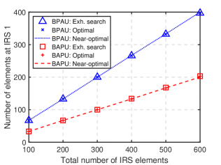
Figure 2: Number of elements at IRS 1 versus total number of elements $N$.

In Fig. 2, we plot the number of elements at IRS 1 versus the total number of reflecting elements $N$. As shown in Fig. 2, the near-optimal solutions proposed in Section III closely match the results obtained by the exhaustive search method, thereby validating their effectiveness. When $N=100$, the optimized elements are $N_{1}=33$ at IRS 1 and $N_{2}=67$ at IRS 2 for BAPU scheme, and $N_{1}=67$ and $N_{2}=33$ for BPAU scheme. The results show that more elements should be deployed at PIRS in both systems, benefiting from its high beamforming gain. When $N=600$, $N_{1}=203$ and $N_{2}=397$ for the BAPU scheme, and $N_{1}=397$ and $N_{2}=203$ for BPAU scheme, which implies that the optimized elements for both IRSs increase with $N$. The results agree with the analysis of Proposition 2 and 3.

V-A2 Impact of Total Number of IRS Elements

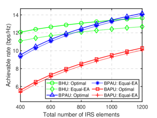
Figure 3: Achievable rate versus total number of elements $N$.

To unveil the benefits of the proposed design, we study the impact of the total number of IRS elements $N$ on the achievable rate, by plotting it versus $N$ in Fig. 3. It is observed that the achievable rates of both BAPU and BPAU schemes grow faster than that of BHU, owing to their higher SNR scaling order (i.e., $\mathcal{O}(N^{3})$ versus $\mathcal{O}(N^{2})$). Moreover, we observe that the optimal IRS elements allocation design outperforms the equal elements allocation, which highlights the importance of determining the number of active and passive elements at the IRS, especially for the BHU scheme. Note that the PIRS should be placed close to the BS or user, while the AIRS prefers to be close to the user. BAPU performs much better than BPAU because it is deployed at an inappropriate location, which motivates us to investigate the impact of IRS placement for further comparison.

V-B IRS Placement Optimization

In this subsection, we first validate the effectiveness of the proposed IRS placement design. Subsequently, we shed light on the rate performance comparison of three IRS deployment schemes. The number of active and passive elements are set as $N_{\mathrm{a}}=200$ and $N_{\mathrm{p}}=500$, respectively. The height of IRS for BHU scheme is set as $h_{\mathrm{s}}=10$ m, and that for BAPU and BPAU scheme is set as $h_{\mathrm{d}}=5$ m. We consider the following schemes: 1) Exh. search: Exhaustive search method is adopted to find the optimal IRS placement without the considered approximations; 2) Middle: The IRS location is fixed where the horizontal distance between BS and AIRS/HIPS is set to $L/2$.

V-B1 Accuracy of IRS Placement Design

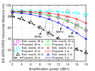
Figure 4: Optimized IRS placement versus amplification power $P_{\mathrm{I}}$.

In Fig. 4, we plot the optimized horizontal distance between BS and AIRS/HIRS versus amplification power at different heights of IRSs. First, one can observe that our proposed near-optimal placement is close to the optimal one obtained by exhaustive search in the cases of different IRS heights, which validates its effectiveness. Second, we observe that the BS-AIRS and BS-HIRS horizontal distance decreases as $P_{\mathrm{I}}$ increases. With a larger $P_{\mathrm{I}}$, the AIRS/HIRS should be deployed closer to the BS to attenuate the channel gain, thereby reducing the noise amplification. Third, it is observed that the height of the IRS has a more significant effect on the optimized horizontal position under the double-reflection case than under the single-reflection case. Specifically, for the BAPU scheme, the AIRS prefers to be closer to the passive IRS to minimize the path loss. Moreover, the two distributed IRSs tend to be closer together for the BPAU scheme and farther apart for the BAPU scheme, which shows the importance of properly designing appropriate placement strategies for the schemes with different deployment orders of AIRS and PIRS.

V-B2 Impact of Amplification Power

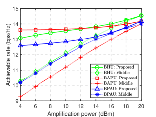
Figure 5: Achievable rate versus amplification power $P_{\mathrm{I}}$.

To show the superiority of the proposed IRS placement design, we study the impact of the amplification power of active elements on the achievable rate, by plotting it versus the amplification power $P_{\mathrm{I}}$ in Fig. 5. First, one can observe that the rates achieved by all the schemes increase with the $P_{\mathrm{I}}$ due to the higher signal amplification gain. Second, it is observed that the proposed IRS placement design can significantly improve the achievable rate compared to the fixed placement strategies. The performance gap is pronounced when the amplification power is small. This is because it enjoys the advantages of dynamically striking a balance between signal and noise amplification at the active elements. Moreover, we observe that the BHU scheme outperforms the BPAU scheme over the whole considered $P_{\mathrm{I}}$ regime, which agrees with our analysis in (44). Furthermore, BHU performs best when $P_{\mathrm{I}}>12$ dBm since it can fully exploit the beamforming and amplification gains provided by active elements. When $P_{\mathrm{I}}=P_{\mathrm{B}}=20$ dBm, it is observed that BAPU and BPAU achieve the same rate performance, which validates our analysis in (45).

V-C Performance Comparison via Joint Optimization

For comparison, we consider the following benchmarks: 1) BPU [6]: The transmission link is BS→PIRS→user, where the PIRS is consists of $N$ passive elements and placed directly above the user; 2) BPPU [38]: The transmission link is BS→PIRS 1→PIRS 2→user, where both PIRSs are deployed directly above the BS and user, respectively, each with $N/2$ passive elements. The height of IRSs are same as those for Fig. (4) and Fig. (5).

V-C1 Impact of Total Number of IRS Elements

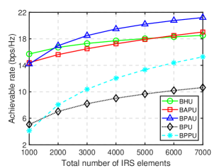
Figure 6: Achievable rate versus total number of elements $N$.

In Fig. 6, the achievable rate versus the total number of IRS elements $N$ is plotted to unveil the impact of the elements budget on the system’s performance. It is observed that BAPU and BPAU perform similarly and are both worse than BHU when the total number of IRS elements is small, which indicates that BHU is a preferred choice for the size-limited case. As $N$ increases, BPAU outperforms BAPU. Moreover, both schemes perform better than BHU because the SNR of systems with the first two schemes increase with $N$ as $\mathcal{O}(N^{3})$ thanks to the IRS elements allocation optimization, whereas that with the latter increases with $N$ as $\mathcal{O}(N^{2})$. The result emphasizes the significance of carefully optimizing the IRS elements allocation to fully exploit the increase in large $N$ for improving the performance of the systems with BAPU or BPAU schemes. Moreover, we observe that the three considered schemes outperform BPPU and BPU schemes when the total number of IRS elements is moderate, which unveils their effectiveness.

V-C2 Impact of Amplification Power

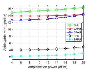
Figure 7: Achievable rate versus amplification power $P_{\mathrm{I}}$.

In Fig. 7, we plot the achievable rate versus amplification power $P_{\mathrm{I}}$. For the entire range of the amplification power, the schemes with active elements outperform those with passive elements only because they provide a high amplification gain. Moreover, BHU achieves the best rate performance under the limited IRS element budget thanks to its optimal IRS elements allocation and placement, which strikes a good balance between the power amplification gain of active elements and the beamforming gain provided by the passive elements. Since the HIRS comprises both active and passive elements, the multiplicative path loss effect can be effectively alleviated via the flexible elements allocation compared to the single/double PIRS.

Note that AIRS can effectively mitigate the multiplicative fading effect. When $P_{\mathrm{I}}$ is small, BAPU performs better than BPAU because it suffers less path loss over shorter signal propagation distance. However, the achievable rate of BAPU remains almost constant under different amplification power. It inspires us to focus on the configuration of other parameters rather than the amplification power when applying BAPU with optimal IRS elements allocation and placement. BAPU and BPAU achieve the same achievable rate when $P_{\mathrm{I}}=P_{\mathrm{B}}$, which also agrees with our theoretical analysis for the IRS placement optimization. It indicates that the performance bottleneck of BPAU mainly lies in the insufficient amplification power. As such, increasing the amplification coefficient at each element of AIRS by increasing the amplification power budget can compensate for the performance loss caused by the limited total number of IRS elements with the BPAU scheme. The results highlight the importance of the placement order of distributed AIRS and PIRS to compensate for the path loss.

V-C3 Impact of Transmit Power

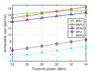
Figure 8: Achievable rate versus transmit power $P_{\mathrm{B}}$.

In Fig. 8, we investigate the impact of transmit power on achievable rate by plotting it versus transmit power $P_{\mathrm{B}}$. One can observe that BHU performs better than other schemes when $P_{\mathrm{B}}<30$ dBm. It demonstrates the superiority of the HIRS and implies that the deployment of HIRS is beneficial for practical scenarios with a limited budget for the total number of IRS elements, amplification power, and transmit power. As $P_{\mathrm{B}}$ increases, the achievable rates of all the schemes increase because of the increasing beamforming gain brought by the IRS. However, the increase in transmit power leads to a decrease in the reflection coefficient, which severely limits the performance of the single-reflection link involving active elements in an HIRS-aided communication system. This is also the reason why the corresponding curve tends to converge when the transmission power is large. Compared to increasing the amplification power, increasing the transmission power has a greater effect on enhancing the rate performance, especially for the BAPU scheme. When $P_{\mathrm{B}}>30$ dBm, we observe that the BAPU becomes the best choice for achievable rate maximization. This is because it not only provides a higher beamforming gain through double reflections but also enables a flexible balance between signal and noise amplification at the AIRS. The results highlight the importance of appropriately configuring the transmit power for BAPU to fully harness its potential for enhancing rate performance.

VI Conclusion

In this paper, we studied the capacity of the IRS-aided communication system with both active and passive elements. In particular, three deployment schemes were considered, namely, BHU, BAPU, and BPAU schemes. The optimized elements allocation and placement design for the three schemes was provided, which lays the foundation for theoretical performance comparison. Our analysis revealed that more passive elements should be deployed under the BAPU and BPAU schemes. Moreover, the HIRS/AIRS should be placed closer to the BS as the amplification power increases. With the proposed joint design of the IRS elements allocation and placement, the BHU scheme can be a practically promising solution for maximizing the capacity and enabling energy-efficient communication in space-limited scenarios. In contrast, BAPU achieves better rate performance with sufficient transmit power, whereas BPAU is preferable for a large total number of IRS elements. Numerical results validated the theoretical findings and demonstrated that our proposed systems outperform other benchmark systems in terms of achievable rate under different system setups.

To facilitate the derivation of IRS deployment for rate performance comparison under different transmission schemes, we assume that the BS is equipped with a single antenna and the transmit power is fixed for tractability, as in [16, 52, 55]. The results in this paper can be extended to the multi-antenna BS case in principle, however, dedicated algorithms are needed to optimize the transmit power/beamformer [56, 42], which is left for our future work. With a higher transmit beamforming gain, it might be the case that more passive elements should be allocated at the HIRS to capture a higher passive beamforming gain, whereas more active elements should be deployed to increase the amplification gain under the BAPU/BPAU scheme. Moreover, it would be likely that the HIRS/AIRS moves closer to the user. By jointly designing the elements allocation and placement, the BAPU scheme may outperform the other two schemes. In addition, this paper can be extended in several promising directions to motivate future work. For example, the real effects of multi-path wireless environment can be more accurately characterized by considering the non-LoS paths, which is beneficial for further improving the IRS deployment design. Furthermore, it is worth investigating the impact of IRSs in the scenario with direct BS-user link.

Appendix A: Proof of Proposition 1

Note that ${\gamma_{0}}$ is a function w.r.t. $\tilde{N}_{\mathrm{a}}$ and thus we use $\gamma_{\mathrm{h}}({{{\tilde{N}}_{{\mathrm{a}}}}})={c_{1}}{\left({{c_{2}}\sqrt{{\tilde{N}_{{\mathrm{a}}}}}+{N_{{\mathrm{p}}}}}\right)^{2}}$ to represent ${\gamma_{0}}$. The first-order partial derivative of $\gamma_{\mathrm{h}}({{{\tilde{N}}_{{\mathrm{a}}}}})$ w.r.t. $\sqrt{\tilde{N}_{\mathrm{a}}}$ is given by

$$\frac{{\partial\gamma_{\mathrm{h}}({{{\tilde{N}}_{{\mathrm{a}}}}})}}{{\partial\sqrt{{{\tilde{N}}_{{\mathrm{a}}}}}}}\!=2{c_{1}}({-{{\tilde{N}}_{{\mathrm{a}}}}+{c_{2}}\sqrt{{{\tilde{N}}_{{\mathrm{a}}}}}+N})({-2\sqrt{{{\tilde{N}}_{{\mathrm{a}}}}}+{c_{2}}}).$$ (59)

Note that ${c_{1}}>0$. Moreover, we have ${-{{\tilde{N}}_{{\mathrm{a}}}}+{c_{2}}\sqrt{{{\tilde{N}}_{{\mathrm{a}}}}}+N}>0,\forall\sqrt{\tilde{N}_{\mathrm{a}}}$ since $\alpha_{\mathrm{0}}\geq 1$, i.e., $c_{2}\geq\sqrt{\tilde{N}_{\mathrm{a}}}$. Thus, the roots for (59) are give by $\sqrt{\tilde{N}_{\mathrm{a}}}=x_{\mathrm{0,rt}}\buildrel\Delta\over{=}{c_{2}}/2$. When $\sqrt{\tilde{N}_{\mathrm{a}}}\leq x_{\mathrm{0,rt}}$, it follows that $\frac{{\partial\gamma_{\mathrm{h}}({{{\tilde{N}}_{{\mathrm{a}}}}})}}{{\partial\sqrt{{{\tilde{N}}_{{\mathrm{a}}}}}}}>0$, i.e., $\gamma_{\mathrm{h}}({{{\tilde{N}}_{{\mathrm{a}}}}})$ monotonically increases with ${{{\tilde{N}}_{{\mathrm{a}}}}}$. Thus, $\gamma_{\mathrm{h}}({{{\tilde{N}}_{{\mathrm{a}}}}})$ is maximized at $\tilde{N}_{\mathrm{a}}=N-1$. Otherwise, it follows that $\frac{{\partial\gamma_{\mathrm{h}}({{{\tilde{N}}_{{\mathrm{a}}}}})}}{{\partial\sqrt{{{\tilde{N}}_{{\mathrm{a}}}}}}}>0,\forall{{{\tilde{N}}_{{\mathrm{a}}}}}\in(0,x_{\mathrm{0,rt}}^{2})$ and $\frac{{\partial\gamma_{\mathrm{h}}({{{\tilde{N}}_{{\mathrm{a}}}}})}}{{\partial\sqrt{{{\tilde{N}}_{{\mathrm{a}}}}}}}<0,\forall{{{\tilde{N}}_{{\mathrm{a}}}}}\in(x_{\mathrm{0,rt}}^{2},N)$, which implies that $\gamma_{\mathrm{h}}({{{\tilde{N}}_{{\mathrm{a}}}}})$ first increases and then decreases with ${{{\tilde{N}}_{{\mathrm{a}}}}}$. Thus, $\gamma_{\mathrm{h}}({{{\tilde{N}}_{{\mathrm{a}}}}})$ is maximized at $\tilde{N}_{\mathrm{a}}=x_{\mathrm{0,rt}}^{2}$. Based on the above results, we complete the proof.

Appendix B: Proof of Proposition 2

Note that ${\gamma_{1}}$ is a function w.r.t. $\tilde{N}_{\mathrm{p}}$ and thus we use $\gamma_{\mathrm{ap}}({{{\tilde{N}}_{{\mathrm{p}}}}})=\frac{{{c_{6}}{N_{{\mathrm{a}}}}\tilde{N}_{{\mathrm{p}}}^{2}}}{{{c_{3}}\tilde{N}_{{\mathrm{p}}}^{2}+{c_{4}}}}$ to represent ${\gamma_{1}}$, where the first-order partial derivative of $\gamma_{\mathrm{ap}}({{{\tilde{N}}_{{\mathrm{p}}}}})$ w.r.t. $\tilde{N}_{\mathrm{p}}$ is given by

$$\frac{{\partial{\gamma_{\mathrm{ap}}({{{\tilde{N}}_{{\mathrm{p}}}}})}}}{{\partial{{\tilde{N}}_{{\mathrm{p}}}}}}=\frac{{{c_{6}}{{\tilde{N}}_{{\mathrm{p}}}}({-{c_{3}}\tilde{N}_{{\mathrm{p}}}^{3}-3{c_{4}}{{\tilde{N}}_{{\mathrm{p}}}}+2N{c_{4}}})}}{{{{({{c_{3}}\tilde{N}_{{\mathrm{p}}}^{2}+{c_{4}}})^{2}}}}}.$$ (60)

Let $x={\tilde{N}}_{{\mathrm{p}}}$ and $g_{1}\left(x\right)\buildrel\Delta\over{=}{-{c_{3}}x^{3}-3{c_{4}}x+2N{c_{4}}}$. The first-order partial derivative of $g_{1}\left(x\right)$ w.r.t. $x$ is given by $g_{1}^{\prime}\left(x\right)=-3{c_{3}}x^{2}-3{c_{4}}$. Since $g_{1}^{\prime}\left(x\right)<0$ for $x\in\left[0,N\right]$, $g_{1}\left(x\right)$ monotonically decreases with $x$ for $x\in\left[0,N\right]$. Hence, the single unique root of $g_{1}\left(x\right)=0$ is denoted by $x_{1}^{\mathrm{rt}}$. When $x\in[0,x_{1}^{\mathrm{rt}})$, we have $g_{1}\left(x\right)>0$ and $\frac{{\partial{\gamma_{\mathrm{ap}}({{{\tilde{N}}_{{\mathrm{p}}}}})}}}{{\partial{{\tilde{N}}_{{\mathrm{p}}}}}}>0$, which implies that $\gamma_{\mathrm{ap}}({{{\tilde{N}}_{{\mathrm{p}}}}})$ monotonically increases with ${\tilde{N}}_{{\mathrm{p}}}$. When $x\in(x_{1}^{\mathrm{rt}},N]$, it follows that $g_{1}\left(x\right)<0$ and $\frac{{\partial{\gamma_{\mathrm{ap}}({{{\tilde{N}}_{{\mathrm{p}}}}})}}}{{\partial{{\tilde{N}}_{{\mathrm{p}}}}}}<0$, i.e., $\gamma_{\mathrm{ap}}({{{\tilde{N}}_{{\mathrm{p}}}}})$ monotonically decreases with ${\tilde{N}}_{{\mathrm{p}}}$. Accordingly, $\gamma_{\mathrm{ap}}({{{\tilde{N}}_{{\mathrm{p}}}}})$ is maximized when ${\tilde{N}}_{{\mathrm{p}}}=x_{1}^{\mathrm{rt}}$. Proposition 2 is thus proved.

Appendix C: Proof of Proposition 4

The first-order partial derivative of ${\gamma_{{\mathrm{0,x}}}}(x_{\mathrm{BI}})$ w.r.t. $x_{\mathrm{BI}}$ is given by

$$\frac{{\partial{\gamma_{{\mathrm{0,x}}}}(\!{{x_{{\mathrm{BI}}}}}\!)}}{{\partial{x_{{\mathrm{BI}}}}}}\!\!=\!\!\frac{{-2N_{{\mathrm{p}}}^{2}P_{\mathrm{B}}^{3}{\beta^{3}}{x_{{\mathrm{BI}}}}{{({\sqrt{{N_{{\mathrm{a}}}}{P_{\mathrm{I}}}}\!\!+\!\!{f_{1}}(\!{{x_{{\mathrm{BI}}}}}\!)})^{3}}}{f_{2}}(\!{{x_{{\mathrm{BI}}}}}\!)}}{{{{({x_{{\mathrm{BI}}}^{2}+h_{\mathrm{s}}^{2}})^{2}}}{f_{1}}({{x_{{\mathrm{BI}}}}})f_{3}^{2}({{x_{{\mathrm{BI}}}}})}},$$ (61)

where ${f_{1}}\left({{x_{{\mathrm{BI}}}}}\right)=\sqrt{N_{{\mathrm{p}}}^{2}{P_{\mathrm{B}}}\beta/\left({x_{{\mathrm{BI}}}^{2}+h_{\mathrm{s}}^{2}}\right)}$,

$${f_{2}}\left({{x_{{\mathrm{BI}}}}}\right)= \frac{{{{\left({x_{{\mathrm{BI}}}^{2}+h_{\mathrm{s}}^{2}}\right)^{2}}}{f_{1}}\left({{x_{{\mathrm{BI}}}}}\right)\left({{c_{10}}{x_{{\mathrm{BI}}}}-{c_{9}}\left({L-{x_{{\mathrm{BI}}}}}\right)}\right)}}{{N_{{\mathrm{p}}}^{2}P_{\mathrm{B}}^{2}{\beta^{2}}{x_{{\mathrm{BI}}}}\left({\sqrt{{N_{{\mathrm{a}}}}{P_{\mathrm{I}}}}+{f_{1}}\left({{x_{{\mathrm{BI}}}}}\right)}\right)}}$$

$$+\frac{{{f_{3}}\left({{x_{{\mathrm{BI}}}}}\right)}}{{{P_{\mathrm{B}}}\beta{{\left({\sqrt{{N_{{\mathrm{a}}}}{P_{\mathrm{I}}}}+{f_{1}}\left({{x_{{\mathrm{BI}}}}}\right)}\right)^{2}}}}},$$ (62)

${f_{3}}\left({{x_{{\mathrm{BI}}}}}\right)={c_{10}}\left({x_{{\mathrm{BI}}}^{2}+h_{\mathrm{s}}^{2}}\right)+{c_{9}}\left({{{\left({L-{x_{{\mathrm{BI}}}}}\right)^{2}}}+h_{\mathrm{s}}^{2}}\right)$. In the high SNR case, i.e., ${{{P_{\mathrm{B}}}\beta{{\left({\sqrt{{N_{{\mathrm{a}}}}{P_{\mathrm{I}}}}+{f_{1}}\left({{x_{{\mathrm{BI}}}}}\right)}\right)^{2}}}}}/{{{f_{3}}\left({{x_{{\mathrm{BI}}}}}\right)}}\gg 1$, we have ${f_{3}}\left({{x_{{\mathrm{BI}}}}}\right)/\left({{P_{\mathrm{B}}}\beta{{\left({\sqrt{{N_{{\mathrm{a}}}}{P_{\mathrm{I}}}}+{f_{1}}\left({{x_{{\mathrm{BI}}}}}\right)}\right)^{2}}}}\right)\ll 1$, which can be approximated as 0. Hence, the single unique root of ${f_{2}}\left({{x_{{\mathrm{BI}}}}}\right)$ is denoted by $x_{{\mathrm{BI}}}^{\mathrm{rt}}=c_{9}L/(c_{9}+c_{10})$. When $x_{{\mathrm{BI}}}\in[0,x_{{\mathrm{BI}}}^{\mathrm{rt}})$, we have ${f_{2}}\left({{x_{{\mathrm{BI}}}}}\right)<0$ and $\frac{{\partial{\gamma_{{\mathrm{0,x}}}}({{x_{{\mathrm{BI}}}}})}}{{\partial{x_{{\mathrm{BI}}}}}}>0$, which implies that ${{\gamma_{{\mathrm{0,x}}}}\left({{x_{{\mathrm{BI}}}}}\right)}$ monotonically increases with $x_{{\mathrm{BI}}}$. When $x_{{\mathrm{BI}}}\in(x_{{\mathrm{BI}}}^{\mathrm{rt}},L]$, it follows that ${f_{2}}\left({{x_{{\mathrm{BI}}}}}\right)>0$ and $\frac{{\partial{\gamma_{{\mathrm{0,x}}}}({{x_{{\mathrm{BI}}}}})}}{{\partial{x_{{\mathrm{BI}}}}}}<0$, i.e., ${{\gamma_{{\mathrm{0,x}}}}\left({{x_{{\mathrm{BI}}}}}\right)}$ monotonically decreases with $x_{{\mathrm{BI}}}$. Thus, ${{\gamma_{{\mathrm{0,x}}}}\left({{x_{{\mathrm{BI}}}}}\right)}$ is maximized at $x_{{\mathrm{BI}}}=x_{{\mathrm{BI}}}^{\mathrm{rt}}$, which completes the proof.

References

- [1] Q. Wu et al., “Intelligent surfaces empowered wireless network: Recent advances and the road to 6G,” Proc. IEEE, vol. 112, no. 7, pp. 724–763, Jul. 2024.
- [2] G. Chen et al., “IRS aided MEC systems with binary offloading: A unified framework for dynamic IRS beamforming,” IEEE J. Sel. Areas Commun., vol. 41, no. 2, pp. 349–365, Feb. 2023.
- [3] R. Liu, M. Li, Y. Liu, Q. Wu, and Q. Liu, “Joint transmit waveform and passive beamforming design for RIS-aided DFRC systems,” IEEE J. Sel. Top. Signal Process., vol. 16, no. 5, pp. 995–1010, Aug. 2022.
- [4] M. Hua et al., “Secure intelligent reflecting surface-aided integrated sensing and communication,” IEEE Trans. Wirel. Commun., vol. 23, no. 1, pp. 575–591, Jan. 2024.
- [5] G. Chen et al., “Intelligent reflecting surface aided MIMO networks: Distributed or centralized architecture?” arXiv preprint arXiv:2310.01742, 2023.
- [6] Q. Wu and R. Zhang, “Intelligent reflecting surface enhanced wireless network via joint active and passive beamforming,” IEEE Trans. Wirel. Commun., vol. 18, no. 11, pp. 5394–5409, Nov. 2019.
- [7] Y. Zhao, Q. Wu, W. Chen, C. Wu, and H. V. Poor, “Performance-oriented design for intelligent reflecting surface-assisted federated learning,” IEEE Trans. Commun., vol. 71, no. 9, pp. 5228–5243, Sep. 2023.
- [8] R. Liu, Q. Wu, M. D. Renzo, and Y. Yuan, “A path to smart radio environments: An industrial viewpoint on reconfigurable intelligent surfaces,” IEEE Wirel. Commun., vol. 29, no. 1, pp. 202–208, Feb. 2022.
- [9] X. Guan and Q. Wu, “IRS-enabled spectrum sharing: Interference modeling, channel estimation and robust passive beamforming,” ZTE Communications, vol. 20, no. 1, pp. 28–35, Mar. 2022.
- [10] Z. Shao, W. Yan, and X. Yuan, “Markovian cascaded channel estimation for RIS aided massive MIMO using 1-bit ADCs and oversampling,” ZTE Communications, vol. 20, no. 1, pp. 48–56, Mar. 2022.
- [11] M. Jian, N. Zhang, and Y. Chen, “RIS: Spatial-wideband effect analysis and off-grid channel estimation,” ZTE Communications, vol. 20, no. 1, pp. 57–62, Mar. 2022.
- [12] R. Long, Y. Liang, Y. Pei, and E. G. Larsson, “Active reconfigurable intelligent surface-aided wireless communications,” IEEE Trans. Wirel. Commun., vol. 20, no. 8, pp. 4962–4975, Aug. 2021.
- [13] G. Chen, Q. Wu, C. He, W. Chen, J. Tang, and S. Jin, “Active IRS aided multiple access for energy-constrained IoT systems,” IEEE Trans. Wireless Commun., vol. 22, no. 3, pp. 1677–1694, Mar. 2023.
- [14] K. Zhi, C. Pan, H. Ren, K. K. Chai, and M. Elkashlan, “Active RIS versus passive RIS: Which is superior with the same power budget?” IEEE Commun. Lett., vol. 26, no. 5, pp. 1150–1154, May 2022.
- [15] Y. Gao et al., “Beamforming optimization for active intelligent reflecting surface-aided SWIPT,” IEEE Trans. Wirel. Commun., vol. 22, no. 1, pp. 362–378, Jan. 2023.
- [16] Z. Kang et al., “Active-passive IRS aided wireless communication: New hybrid architecture and elements allocation optimization,” IEEE Trans. Wirel. Commun., vol. 23, no. 4, pp. 3450–3464, Aug. 2024.
- [17] Q. Peng, Q. Wu, G. Chen, R. Liu, S. Ma, and W. Chen, “Hybrid active-passive IRS assisted energy-efficient wireless communication,” IEEE Commun. Lett., vol. 27, no. 8, pp. 2202–2206, Jul. 2023.
- [18] A. Huang, X. Mu, L. Guo, and G. Zhu, “Hybrid active-passive RIS transmitter enabled energy-efficient multi-user communications,” IEEE Trans. Wireless Commun., vol. 23, no. 9, pp. 10 653–10 666, Sep. 2024.
- [19] L. Zhuang, J. Zhu, Z. Zhang, and F. Fang, “Hybrid active-passive intelligent reflecting surface for secure communication,” in Proc. IEEE GLOBECOM, Kuala Lumpur, Malaysia, Dec. 2023, pp. 2711–2716.
- [20] W. Hao, Y. Qu, S. Zhou, F. Wang, Z. Lu, and S. Yang, “Joint beamforming design for hybrid RIS-assisted mmwave ISAC system relying on hybrid precoding structure,” IEEE Internet Things J., vol. 11, no. 18, pp. 29 455–29 469, Sep. 2024.
- [21] N. T. Nguyen, Q. Vu, K. Lee, and M. J. Juntti, “Hybrid relay-reflecting intelligent surface-assisted wireless communications,” IEEE Trans. Veh. Technol., vol. 71, no. 6, pp. 6228–6244, Jun. 2022.
- [22] N. T. Nguyen et al., “Hybrid active-passive reconfigurable intelligent surface-assisted multi-user MISO systems,” in Proc. IEEE 23rd Int. Workshop Signal Process. Adv. Wireless Commun. (SPAWC), Jul. 2022, pp. 1–5.
- [23] M. Hua et al., “Intelligent reflecting surface-assisted localization: Performance analysis and algorithm design,” IEEE Wirel. Commun. Lett., vol. 13, no. 1, pp. 84–88, Jan. 2024.
- [24] Q. Peng, Q. Wu, W. Chen, S. Ma, M.-M. Zhao, and O. A. Dobre, “Semi-passive intelligent reflecting surface enabled sensing systems,” 2024, Early Access, doi:10.1109/TCOMM.2024.3399202.
- [25] B. Zheng, C. You, and R. Zhang, “Double-IRS assisted multi-user MIMO: Cooperative passive beamforming design,” IEEE Trans. Wirel. Commun., vol. 20, no. 7, pp. 4513–4526, Feb. 2021.
- [26] C. You, B. Zheng, and R. Zhang, “Wireless communication via double IRS: Channel estimation and passive beamforming designs,” IEEE Wirel. Commun. Lett., vol. 10, no. 2, pp. 431–435, Oct. 2021.
- [27] Y. Han, S. Zhang, L. Duan, and R. Zhang, “Double-IRS aided MIMO communication under LoS channels: Capacity maximization and scaling,” IEEE Trans. Commun., vol. 70, no. 4, pp. 2820–2837, Apr. 2022.
- [28] W. Mei and R. Zhang, “Multi-beam multi-hop routing for intelligent reflecting surfaces aided massive MIMO,” IEEE Trans. Wirel. Commun., vol. 21, no. 3, pp. 1897–1912, Mar. 2022.
- [29] Y. Zhang, C. You, and B. Zheng, “Multi-active multi-passive (MAMP)-IRS aided wireless communication: A multi-hop beam routing design,” IEEE J. Sel. Areas Commun., vol. 41, no. 8, pp. 2497–2513, Aug. 2023.
- [30] W. Mei and R. Zhang, “Distributed beam training for intelligent reflecting surface enabled multi-hop routing,” IEEE Wirel. Commun. Lett., vol. 10, no. 11, pp. 2489–2493, Nov. 2021.
- [31] F. Naeem, G. Kaddoum, S. Khan, K. S. Khan, and N. H. Adam, “IRS-empowered 6G networks: Deployment strategies, performance optimization, and future research directions,” IEEE Access, vol. 10, pp. 118 676–118 696, Nov. 2022.
- [32] W. Mei and R. Zhang, “Cooperative beam routing for multi-IRS aided communication,” IEEE Wirel. Commun. Lett., vol. 10, no. 2, pp. 426–430, Feb. 2021.
- [33] Y. Liu, Y. Ma, M. Li, Q. Wu, and Q. Shi, “Spectral efficiency maximization for double-faced active reconfigurable intelligent surface,” IEEE Trans. Signal Process., vol. 70, pp. 5397–5412, Nov. 2022.
- [34] B. Wang, C. Pan, H. Ren, Z. Yu, Y. Zhang, M. Liu, and G. Zhou, “Beamforming design for double-active-RIS-aided communication systems with inter-excitation,” arXiv preprint arXiv:2403.11061, 2024.
- [35] M. Liu et al., “Joint beamforming design for double active RIS-assisted radar-communication coexistence systems,” IEEE Trans. Cogn. Commun. Netw., vol. 10, no. 5, pp. 1704–1717, Oct. 2024.
- [36] M. Fu and R. Zhang, “Active and passive IRS jointly aided communication: Deployment design and achievable rate,” IEEE Wirel. Commun. Lett., vol. 12, no. 2, pp. 302–306, Feb. 2023.
- [37] C. Huang, W. Chen, and Q. Wu, “Joint active and passive IRS aided wireless communication: Elements allocation and achievable rate,” arXiv preprint arXiv:2404.06880, 2024.
- [38] Y. Han et al., “Cooperative double-IRS aided communication: Beamforming design and power scaling,” IEEE Wirel. Commun. Lett., vol. 9, no. 8, pp. 1206–1210, Aug. 2020.
- [39] H. Xie, B. Gu, and D. Li, “Exploring hybrid active-passive RIS-aided MEC systems: From the mode-switching perspective,” IEEE Trans. Wireless Commun., vol. 23, no. 9, pp. 11 291–11 308, Sep. 2024.
- [40] Q. Wu, S. Zhang, B. Zheng, C. You, and R. Zhang, “Intelligent reflecting surface-aided wireless communications: A tutorial,” IEEE Trans. Commun., vol. 69, no. 5, pp. 3313–3351, May 2021.
- [41] H. Hashida, Y. Kawamoto, and N. Kato, “Intelligent reflecting surface placement optimization in air-ground communication networks toward 6G,” IEEE Wirel. Commun., vol. 27, no. 6, pp. 146–151, Sep. 2020.
- [42] W. Huang, W. Ding, C. Kai, Y. Yi, and Y. Huang, “Joint placement and beamforming design for IRS-enhanced multiuser MISO systems,” IEEE Trans. Commun., vol. 70, no. 10, pp. 6678–6692, Aug. 2022.
- [43] C. You and R. Zhang, “Wireless communication aided by intelligent reflecting surface: Active or passive?” IEEE Wirel. Commun. Lett., vol. 10, no. 12, pp. 2659–2663, Sep. 2021.
- [44] Z. Kang, C. You, and R. Zhang, “Active-IRS-aided wireless communication: Fundamentals, designs and open issues,” IEEE Wireless Commun., vol. 31, no. 3, pp. 368–374, Jun. 2024.
- [45] W. Mei and R. Zhang, “Joint base station and IRS deployment for enhancing network coverage: A graph-based modeling and optimization approach,” IEEE Trans. Wirel. Commun., vol. 22, no. 11, pp. 8200–8213, Nov. 2023.
- [46] M. Fu, W. Mei, and R. Zhang, “Multi-passive/active-IRS enhanced wireless coverage: Deployment optimization and cost-performance trade-off,” IEEE Trans. Wirel. Commun., vol. 23, no. 8, pp. 9657–9671, Aug. 2024.
- [47] C. N. Efrem and I. Krikidis, “Joint IRS location and size optimization in multi-IRS aided two-way full-duplex communication systems,” IEEE Trans. Wirel. Commun., vol. 22, no. 10, pp. 6518–6533, Feb. 2023.
- [48] Z. Kang, C. You, and R. Zhang, “Double-active-IRS aided wireless communication: Deployment optimization and capacity scaling,” IEEE Wirel. Commun. Lett., vol. 12, no. 11, pp. 1821–1825, Nov. 2023.
- [49] X. Li, C. You, Z. Kang, Y. Zhang, and B. Zheng, “Double-active-IRS aided wireless communication with total amplification power constraint,” IEEE Commun. Lett., vol. 27, no. 10, pp. 2817–2821, Oct. 2023.
- [50] M. Asif, X. Bao, A. Ihsan, W. U. Khan, M. Ahmed, and X. Li, “Securing NOMA 6G communications leveraging intelligent omni-surfaces under residual hardware impairments,” IEEE Internet Things J., vol. 11, no. 14, pp. 25 326–25 336, Jul. 2024.
- [51] M. Asif et al., “Energy-efficient beamforming and resource optimization for STAR-IRS enabled hybrid-noma 6G communications,” IEEE Trans. Green Commun. Netw., vol. 7, no. 3, pp. 1356–1368, Sep. 2023.
- [52] X. Mu, Y. Liu, L. Guo, J. Lin, and R. Schober, “Joint deployment and multiple access design for intelligent reflecting surface assisted networks,” IEEE Trans. Wirel. Commun., vol. 20, no. 10, pp. 6648–6664, Oct. 2021.
- [53] F. Amato et al., “Tunneling RFID tags for long-range and low-power microwave applications,” IEEE J. Radio Freq. Identificat., vol. 2, no. 2, pp. 93–103, Jun. 2018.
- [54] G. Stratidakis et al., “Optimal position and orientation study of reconfigurable intelligent surfaces in a mobile user environment,” IEEE Trans. Antennas Propag., vol. 70, no. 10, pp. 8863–8871, Oct. 2022.
- [55] Y. Zhang, S. R. Khosravirad, X. Chu, and M. A. Uusitalo, “On the IRS deployment in smart factories considering blockage effects: Collocated or distributed?” IEEE Trans. Wirel. Commun., vol. 23, no. 9, pp. 12 084–12 098, Sep. 2024.
- [56] N. U. Saqib et al., “Reconfigurable intelligent surface aided hybrid beamforming: Optimal placement and beamforming design,” IEEE Trans. Wirel. Commun., vol. 23, no. 9, pp. 12 003–12 019, Sep. 2024.