Willblue Hmadark4 TRSC-0001-2024.00

Ma, Ma, and Romero

Dynamic Delivery Pooling

Potential-Based Greedy Matching for Dynamic Delivery Pooling

Hongyao Ma Graduate School of Business, Columbia University, New York, NY 10027, hongyao.ma@columbia.edu Will Ma Graduate School of Business, Columbia University, New York, NY 10027, wm2428@gsb.columbia.edu Matias Romero Graduate School of Business, Columbia University, New York, NY 10027, mer2262@gsb.columbia.edu

We study the problem of pooling together delivery orders into a single trip, a strategy widely adopted by platforms to reduce total travel distance. Similar to other dynamic matching settings, the pooling decisions involve a trade-off between immediate reward and holding jobs for potentially better opportunities in the future. In this paper, we introduce a new heuristic dubbed potential-based greedy ($\mathsf{PB}$), which aims to keep longer-distance jobs in the system, as they have higher potential reward (distance savings) from being pooled with other jobs in the future. This algorithm is simple in that it depends solely on the topology of the space, and does not rely on forecasts or partial information about future demand arrivals. We prove that $\mathsf{PB}$ significantly improves upon a naive greedy approach in terms of worst-case performance on the line. Moreover, we conduct extensive numerical experiments using both synthetic and real-world order-level data from the Meituan platform. Our simulations show that $\mathsf{PB}$ consistently outperforms not only the naive greedy heuristic but a number of benchmark algorithms, including (i) batching-based heuristics that are widely used in practice, and (ii) forecast-aware heuristics that are given the correct probability distributions (in synthetic data) or a best-effort forecast (in real data). We attribute the surprising unbeatability of $\mathsf{PB}$ to the fact that it is specialized for rewards defined by distance saved in delivery pooling.

On-demand delivery, Platform operations, Online algorithms, Dynamic matching

1 Introduction

On-demand delivery platforms have become an integral part of modern life, transforming how consumers search for, purchase, and receive goods from restaurants and retailers. Collectively, these platforms serve more than $1.5$ billion users worldwide, contributing to a global market valued at over $250 billion (statista2024). Growth has continued at a rapid pace— major companies such as DoorDash in the United States and Meituan in China reported approximately 25% year-over-year growth in transaction volume in 2023 (curry2024doordash, scmp2024meituan). Managing this ever-expanding stream of orders poses significant operational challenges, particularly as consumers demand increasingly faster deliveries, and fierce competition compels platforms to continuously improve both operational efficiency and cost-effectiveness.

One strategy for improving efficiency and reducing labor costs is to pool into a single trip multiple orders from the same or nearby restaurants. This is referred to as stacked, grouped, or batched orders, and is advertised to drivers as opportunities for increasing earnings and efficiency (doordash2024batched). The strategy has been generally successful and very widely adopted (deliveroo2022, uberEatsMultiple, grabGroupedJobs). For example, data from Meituan, made public by the 2024 INFORMS TSL Data-Driven Research Challenge, show that more than 85% of orders are pooled, rising to 95% during peak hours and consistently remaining above 50% at all other times (see Figure 1).

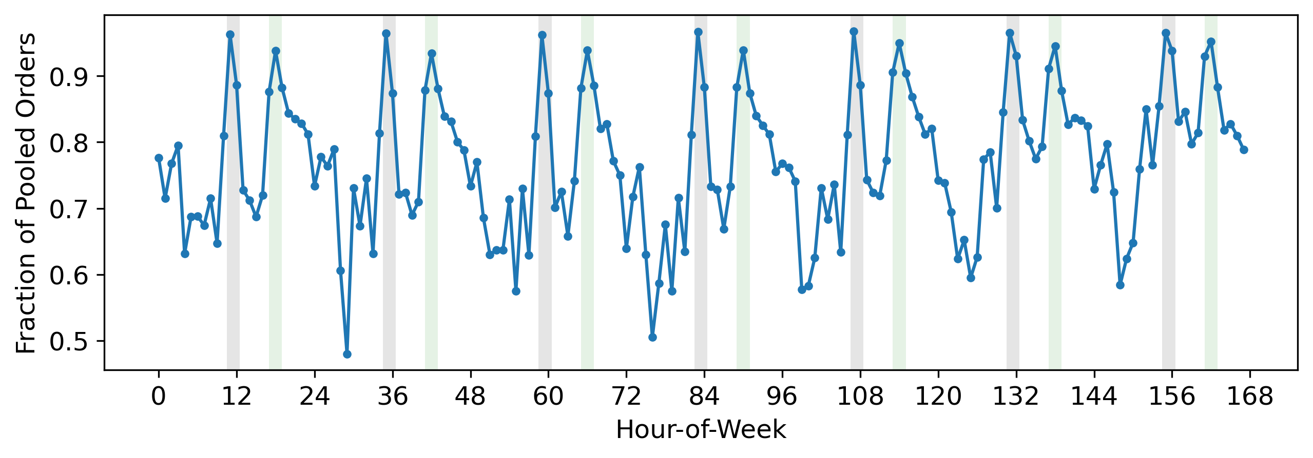
Figure 1: Fraction of pooled orders by hour-of-week in Meituan data. The dataset includes $8$ days of order-level data from one city (see LABEL:sec:sim_meituan for more details). The gray shade indicates peak lunch hours (10:30am-1:30pm), while the green shade indicates peak dinner hours (5pm-8pm).

The delivery pooling approach introduces a highly complex decision-making problem, as orders arrive dynamically to the market, and need to be dispatched within a few minutes — orders in the Meituan data are offered to delivery drivers an average of around five minutes after being placed, often before meal preparation is complete (see LABEL:fig:meituan_order_to_first_dispatch_how). During this limited window of each order, the platform must determine which (if any) of the available orders to pool with, carefully weighing immediate efficiency gains against the uncertain, differential benefits of holding each candidate for future pooling opportunities. Consequently, there remains a pressing need for more efficient and robust solution methods to inform the platform’s delivery pooling decisions.

Similar problems have been studied in the context of various marketplaces such as ride-sharing platforms and kidney exchange programs, in a large body of work known as dynamic matching. However, we argue that the reward structure for delivery pooling is fundamentally different. First, many problems studied in the literature involves connecting two sides of a market, e.g. ridesharing platforms matching drivers to riders. In such bipartite settings, the presence of a large number of agents of identical or similar types (e.g., many riders requesting trips originating from the same area) typically leads to less efficient outcomes. While the kidney exchange problem is not bipartite, long queues of “hard-to-match” patient-donor pairs can still form, when many pairs share the same combination of incompatible tissue types and blood types.

In stark contrast, it is unlikely for long queues to build up for delivery pooling, especially in dense markets, in that given enough orders, two of them will have closely situated origins and destinations, resulting in a good match. In fact, many customers requesting deliveries originating from the same location is actually desirable, since this reduces travel distance and parking stops. We find that delivery orders tend to indeed be highly concentrated in space, with most requests originating from popular restaurants in busy city centers and ending in residential neighborhoods (see LABEL:appx:meituan_spatial_distribution). We emphasize that we are not studying the problem of matching (pooled) orders to couriers, but delivery pooling is a relevant first step regardless, as pooling orders efficiently before matching with couriers will effectively increase the amount of courier capacity.

In this work, we study delivery pooling and exploit its distinct reward topology, that it is highly desirable to match two jobs of identical or very similar types, as described above. We develop a simple ”potential-based” greedy algorithm, which relies solely on the reward topology to determine the opportunity cost of dispatching each job. The intuition behind it is elementary — long-distance jobs have higher potential for cost savings when pooled with other jobs, and hence the online algorithm should generally prefer keeping them in the system, dispatching shorter deliveries first when it has a choice.

1.1 Model Description

Different models of arrivals and departures have been proposed in the dynamic matching literature (see Subsection 1.3.1), and we believe our insight about potential is relevant across all of them. However, in this paper we focus on a single model well-suited for the delivery pooling application.

To elaborate, we consider a dynamic non-bipartite matching problem, with a total of $n$ jobs arriving sequentially to be matched. Jobs are characterized by (potentially infinite) types $\theta\in\Theta$ representing features (e.g. locations of origin and destination) that determine the reward for the platform. Given the motivating application to pooled deliveries, we will always model jobs’ types as belonging to some metric space. Following ashlagi2019edge, we assume that an unmatched job must be dispatched after $d$ new arrivals, which we interpret as a known internal deadline imposed by the platform to incentivize timely service. The platform is allowed to make a last-moment matching decision before the job leaves, termed as the job becoming critical. At this point, the platform must decide either to match the critical job to another available one, collecting reward $r(\theta,\theta^{\prime})$ where $\theta,\theta^{\prime}$ are the types of the matched jobs and $r$ is a known reward function, or to dispatch the critical job on its own for zero reward. The objective is to maximize the total reward collected from matching the $n$ jobs. We believe this to be an appropriate model for delivery platforms (cf. Subsection 1.3.1) because deadlines are known upon arrival and sudden departures (order cancellations) are rare.

Dynamic matching models can also be studied under different forms of information about the future arrivals. Some papers (e.g. kerimov2024dynamic, aouad2020dynamic, eom2023batching, wei2023constant) develop sophisticated algorithms to leverage stochastic information, which is often necessary to derive theoretical guarantees under general matching rewards. In contrast, our heuristic does not require any knowledge of future arrivals, and our theoretical results hold in an ”adversarial” setting where no stochastic assumptions are made. In our experiments, we consider arrivals generated both from stochastic distributions and real-world data, and find that our heuristic can outperform even algorithms that are given the correct stochastic distributions, under our specific reward topology.

1.2 Main Contributions

Notion of potential.

As mentioned above, we design a simple greedy-like algorithm that is based purely on topology and reward structure, which we term potential-based greedy ($\mathsf{PB}$). More precisely, $\mathsf{PB}$ defines the potential of a job type $\theta$ to be $p(\theta)=\sup_{\theta^{\prime}\in\Theta}r(\theta,\theta^{\prime})/2$, measuring the highest-possible reward obtainable from matching type $\theta$. The potential acts as an opportunity cost, and the relevance of this notion arises in settings where the potential is heterogeneous across jobs. To illustrate, let $\Theta=[0,1]$ and $r(\theta,\theta^{\prime})=\min\{\theta,\theta^{\prime}\}$, a reward function used for delivery pooling as we will justify in Section 2. Under this reward function, a job type (which is a real number) can never be matched for reward greater than its real value, which means that jobs with higher real value have greater potential. Our $\mathsf{PB}$ algorithm matches a critical job (with type $\theta$) to the available job (with type $\theta^{\prime}$) that maximizes

$$r(\theta,\theta^{\prime})-p(\theta^{\prime})=\min\{\theta,\theta^{\prime}\}-\frac{1}{2}\theta^{\prime},$$ (1)

being dissuaded to use up job types $\theta^{\prime}$ with high real values. Notably, this definition does not require any forecast or partial information of future arrivals, but rather assumes full knowledge of the universe of possible job types.

Theoretical results.

Our theoretical results assume $\Theta=[0,1]$. We compare $\mathsf{PB}$ to the naive greedy algorithm $\mathsf{GRE}$, which selects $\theta^{\prime}$ to maximize $r(\theta,\theta^{\prime})$, instead of $r(\theta,\theta^{\prime})-p(\theta^{\prime})$ as in (1). We first consider an offline setting ($d=\infty$), showing that under reward function $r(\theta,\theta^{\prime})=\min\{\theta,\theta^{\prime}\}$, our algorithm $\mathsf{PB}$ achieves regret $O(\log n)$, whereas $\mathsf{GRE}$ suffers regret $\Omega(n)$ compared to the optimal matching. Our analysis of $\mathsf{PB}$ is tight, i.e. it has $\Theta(\log n)$ regret. Building upon the offline analysis, we next consider the online setting ($d<n$), showing that $\mathsf{PB}$ has regret $\Theta(\frac{n}{d}\log d)$, which improves as $d$ increases. This can be interpreted as there being $\frac{n}{d}$ ”batches” in the online setting, and our algorithm achieving a regret of $O(\log d)$ per batch. Alternatively, it can be interpreted as the regret per job of our algorithm being $O(\frac{d}{\log d})$. By contrast, we show that the naive greedy algorithm $\mathsf{GRE}$ suffers a total regret of $\Omega(n)$, regardless of $d$.

For comparison, we also analyze two other reward topologies, still assuming $\Theta=[0,1]$.

1. We consider the classical min-cost matching setting (reingold1981greedy) where the goal is to minimize total match distance between points on a line, represented in our model by the reward function $r(\theta,\theta^{\prime})=1-|\theta-\theta^{\prime}|$. For this reward function, both $\mathsf{PB}$ and $\mathsf{GRE}$ have regret $\Theta(\log n)$; in fact, they are the same algorithm because all job types have the same potential. Like before, this translates into both algorithms having regret $\Theta(\frac{n}{d}\log d)$ in the online setting.

2. We consider reward function $r(\theta,\theta^{\prime})=|\theta-\theta^{\prime}|$, representing an opposite setting in which it is worst to match two jobs of the same type. For this reward function, we show that any index-based matching policy must suffer regret $\Omega(n)$ in the offline setting, and that both $\mathsf{PB}$ and $\mathsf{GRE}$ suffer regret $\Omega(n)$ (irrespective of $d$) in the online setting.

Our theoretical results are summarized in Table 1. As our model is a special case of ashlagi2019edge, their 1/4-competitive randomized online edge-weighted matching algorithm can be applied, which essentially translates in our setting to an $O(n)$ upper bound for regret under any definition of reward. Our results show that it is possible to do much better ($O(\log n)$ instead of $O(n)$) for specific reward topologies, using a completely different algorithm and analysis. We now outline how to prove our two main technical results, Theorems 3.3 and LABEL:thm:_dynamic.

$\theta,\theta^{\prime}\in[0,1]$	$r(\theta,\theta^{\prime})=\min\{\theta,\theta^{\prime}\}$	$r(\theta,\theta^{\prime})=1-|\theta-\theta^{\prime}|$	$r(\theta,\theta^{\prime})=|\theta-\theta^{\prime}|$
Regret of $\mathsf{PB}$	Offline: $\Theta(\log n)$
	(Theorem 3.3, LABEL:prop:loglowerboundOffline)
	Online: $\Theta(\frac{n}{d}\log d)$	Offline: $\Theta(\log n)$	Offline: $\Omega(n)$
	(LABEL:thm:_dynamic, LABEL:prop:loglowerboundOnline)	Online: $\Theta(\frac{n}{d}\log d)$	Online: $\Omega(n)$
Regret of $\mathsf{GRE}$	Offline: $\Omega(n)$	(LABEL:sec:reward2)	(LABEL:sec:_reward_3)
	(Proposition 3.2)
	Online: $\Omega(n)$
	(LABEL:prop:greedy_linear_lower_bound_dynamic)

Table 1: Summary of theoretical results under different reward functions $r:[0,1]^{2}\to\mathbb{R}$. The total number of jobs is denoted by $n$, and the batch size in the online setting is approximately $d$.

Proof techniques.

We establish an upper bound on the regret of $\mathsf{PB}$ by comparing its performance to the sum of the potential of all jobs. Under reward function $r(\theta,\theta^{\prime})=\min\{\theta,\theta^{\prime}\}$, the key driver of regret is the sum of the distances between jobs matched by $\mathsf{PB}$. In Theorem 3.3, we study this quantity by analyzing the intervals induced by matched jobs in the offline setting ($d=\infty$). We show that the intervals formed by the matching output of $\mathsf{PB}$ constitute a laminar set family; that is, every two intervals are either disjoint or one fully contains the other. We then prove that more deeply nested intervals must be exponentially smaller in size. Finally, we use an LP to show that the sum of interval lengths remains bounded by a logarithmic function of the number of intervals.

In LABEL:thm:_dynamic, we partition the set of jobs in the online setting into roughly $\frac{n}{d}$ ”batches” and analyze the sum of the distances between matched jobs within a single batch. Our main result is to show that we can use Theorem 3.3 to derive an upper bound for an arbitrary batch. However, a direct application of the theorem on the offline instance defined by the batch would not yield a valid upper bound, because the resulting matching of $\mathsf{PB}$ in the offline setting could be inconsistent with its online matching decisions. To overcome this challenge, we carefully construct a modified offline instance that allows for the online and offline decisions to be coupled, while ensuring that the total matching distance did not go down. This allows us to upper-bound the regret per batch by $O(\log d)$, for a total regret of $O(\frac{n}{d}\log d)$.

Simulations on synthetic data.

We test $\mathsf{PB}$ on random instances in the setting of our theoretical results, except that job types are drawn uniformly at random from $[0,1]$ (instead of adversarial). We benchmark its performance against $\mathsf{GRE}$, as well as more sophisticated algorithms, including (i) batching-based heuristics that are highly relevant both in theory and practice, and (ii) forecast-aware heuristics that use historical data to compute shadow prices. Our extensive simulation results show that $\mathsf{PB}$ consistently outperforms all benchmarks starting from relatively low market densities, achieving over 95% of the hindsight optimal solution that has full knowledge of arrivals. This result is robust to different distributions of job types, and also two-dimensional locations.

Simulations on real data.

Finally, we test the practical applicability of $\mathsf{PB}$ via extensive numerical experiments using order-level data from the Meituan platform, made available from the 2024 INFORMS TSL Data-Driven Research Challenge. The key information we extract from this dataset is the exact timestamps for the creation of each request, and the geographic coordinates of pick-up and drop-off locations. These aspects differ from our theoretical setting in that (i) requests may not be available to be pooled for a fixed number of new arrivals before being dispatched, and (ii) locations are two-dimensional with delivery orders having heterogeneous origins. To address (i), we assume that the platform sets a fixed time window after which an order becomes critical, corresponding to each job being able to wait for at most a fixed sojourn time before being dispatched. For (ii), we extend our definition of reward (that captures the travel distance saved) to two-dimensional heterogeneous origins. Under this new reward definition, the main insight from our theoretical model remains true: longer deliveries have higher potential reward from being pooled with other jobs in the future, and thus $\mathsf{PB}$ aims to keep them in the system.

In contrast to our simulations with synthetic data, the real-life delivery locations may now be correlated and exhibit time-varying effects. Regardless, we find that $\mathsf{PB}$ outperforms all tested heuristics (those without foreknowledge of the future), given that the platform is willing to wait up to one minute before dispatching each job, a fairly modest ask. In this regime, $\mathsf{PB}$ achieves over 80% of the maximum possible travel distance saved from pooling. $\mathsf{PB}$ also pools 10% more jobs than the hindsight optimal matching (see LABEL:sec:match_rate).

Explanation for the surprising unbeatability of $\mathsf{PB}$.

Our potential-based greedy heuristic consistently performs at or near the best across a wide range of experimental setups, including both synthetic and real data. This result is surprising to us, given that $\mathsf{PB}$ is a simple index-based rule that ignores forecast information. To provide some explanation for this finding, we analyze a stylized setting in LABEL:sec:_interpretation, where we show that the ”correct” shadow prices converge to our notion of potential as the market thickness increases. That being said, we also end with a couple of caveats. First, our findings about the effectiveness of $\mathsf{PB}$ are specific to our definition of matching reward for delivery pooling, based on travel distance saved, and may not extend to setting with different reward structures. Second, while we carefully tuned the batching-based and dual-based heuristics that we compare against, it remains possible that more sophisticated algorithms, particularly those leveraging dynamic programming in stochastic settings, could outperform $\mathsf{PB}$.

1.3 Further Related Work

1.3.1 Dynamic matching.

Dynamic matching problems have received growing attention from different communities in economics, computer science, and operations research. We discuss different ways of modeling the trade-off between matching now vs. waiting for better matches, depending on the application that motivates the study.

One possible model (kerimov2024dynamic, kerimov2023optimality, wei2023constant) is to consider a setting with jobs that arrive stochastically in discrete time and remain in the market indefinitely, but use a notion of all-time regret that evaluates a matching policy, at every time period, against the best possible decisions until that moment, to disincentivize algorithms from trivially delaying until the end to make all matches.

A second possible model, motivated by the risk of cancellation in ride-sharing platforms, is to consider sudden departures modeled by jobs having heterogeneous sojourn times representing the maximum time that they stay in the market (aouad2020dynamic). These sojourn times are unknown to the platform, and delaying too long risks many jobs being lost without a chance of being matched. aouad2020dynamic formulates an MDP with jobs that arrive stochastically in continuous time, and leave the system after an exponentially distributed sojourn time. They propose a policy that achieves a multiplicative factor of the hindsight optimal solution. Related work on the control of matching queues with abandonment includes collina2020dynamic, castro2020matching, wang2024demand, kohlenberg2024cost.

A third possible model (huang2018match) also considers jobs that can leave the system at any period, but allows the platform to make a last-moment matching decision right before a job leaves, termed as the job becoming critical. In this model, one can without loss assume that all matching decisions are made at times that jobs become critical.

Finally, the model we study also makes all decisions at times that jobs become critical, with the difference being that the sojourn times are known upon the arrival of a job, as studied in ashlagi2019edge, eom2023batching. Under these assumptions, eom2023batching assume stationary stochastic arrivals, while ashlagi2019edge allow for arbitrary arrivals. Our research focuses on deterministic greedy-like algorithms that can achieve good performance as the market thickness increases. Moreover, our work differs from these papers in the description of the matching value. While they assume arbitrary matching rewards, we consider specific reward functions known to the platform in advance, and use this information to derive a simple greedy-like algorithm with good performance. This aligns with a stream of literature on online matching, that captures more specific features into the model to get stronger guarantees (see kanoria2021dynamic, chen2023feature, balkanski2023power).

We should note that our paper also relates to a recent stream of work studying the effects of batching and delayed decisions in online matching (e.g. feng2024batching, xie2023benefits), as well as works studying the relationship between market thickness and quality of online matches (e.g. ashlagi2021kidney, chen2021matchmaking).

1.3.2 Delivery operations.

On-demand delivery operations have received special attention in the field of transportation and operations management. reyes2018meal introduce the meal delivery routing problem, which falls in the class of dynamic vehicle routing problems (see e.g. psaraftis2016dynamic); the authors develop heuristics to dynamically assign orders to vehicles. Similar efforts have been devoted to optimize detailed pooling and assignment strategies as customer orders arrive sequentially (steever2019dynamic, ulmer2021restaurant), mainly using approximate dynamic programming techniques. These heuristics are shown to work well in extensive numerical experiments, but given the intricate nature of the model and techniques, it is very challenging to derive managerial insights or theoretical performance guarantees. Closer to our research goal, chen2024courier analyze the optimal dispatching policy on a stylized queueing model representing a disk service area centered at one restaurant. They show that delivering multiple orders per trip is beneficial when the service area is large. cachon2023fast study the interplay between the number of couriers and platform efficiency, assuming a one-dimensional geography with one single origin, which is also the primary model in our theoretical results. A similar topology is studied in the game-theoretic model of keskin2024order to capture the impact of delivery pooling on the interaction between the platform, customers, riders, and restaurants.

2 Preliminaries

In this section, we introduce a dynamic non-bipartite matching model for the delivery pooling problem. A total of $n$ jobs arrive to the platform sequentially. Each job $j\in[n]=\{1,\ldots,n\}$, indexed in the order of arrival, has a type $\theta_{j}\in\Theta$. We adopt the criticality assumption from ashlagi2019edge, in the sense that each job remains available to be matched for $d\geq 1$ new arrivals, after which it becomes critical. The parameter $d$ can also be interpreted as the market density. When a job becomes critical, the platform decides whether to (irrevocably) match it with another available job, in which case they are dispatched together (i.e. pooled) and the platform collects a reward given by a known function $r:\Theta^{2}\to\mathbb{R}$. If a critical job is not pooled with another job, it has to be dispatched by itself for zero reward.

2.1 Reward Topology

Our modeling approach directly imposes structure on the type space, as well as the reward function that captures the benefits from pooling delivery orders together. Similar to previous numerical work on pooled trips in ride-sharing platforms (eom2023batching, aouad2020dynamic), we assume that the platform’s goal is to reduce the total distance that needs to be traveled to complete all deliveries. The reward of pooling two orders together is therefore the travel distance saved when they are delivered by the same driver in comparison to delivered separately. Formally, we consider a linear city model where job types $\theta\in\Theta=[0,1]$ represent destinations of the delivery orders, and assume that all orders need to be served from the origin 0 (similar to that analyzed in cachon2023fast) If a job of type $\theta$ is dispatched by itself, the total travel distance from the origin 0 is exactly $\theta$. If it is matched with another job of type $\theta^{\prime}$, they are pooled together on a single trip to the farthest destination $\max\{\theta,\theta^{\prime}\}$. Thus, the distance saved by pooling is

$$r(\theta,\theta^{\prime})=\theta+\theta^{\prime}-\max\{\theta,\theta^{\prime}\}=\min\{\theta,\theta^{\prime}\}.$$ (2)

Although our main theoretical results leverage the structure of this reward topology, our proposed algorithm can be applied to other reward topologies. In particular, we derive theoretical results for two other reward structures for $\Theta=[0,1]$. First, we consider

$$r(\theta,\theta^{\prime})=1-|\theta-\theta^{\prime}|$$ (3)

to capture the commonly-studied spatial matching setting (e.g. kanoria2021dynamic, balkanski2023power), where the reward is larger if the distance $|\theta-\theta^{\prime}|$ is smaller. We also consider

$$r(\theta,\theta^{\prime})=|\theta-\theta^{\prime}|$$ (4)

with the goal of matching types that are far away from each other, contrasting the other two reward functions. In addition, we perform numerical experiments for delivery pooling in two-dimensional (2D) space, where the reward function corresponds to the travel distance saved in the 2D setting.

2.2 Benchmark Algorithms

Given market density $d$ and reward function $r$, if the platform had full information of the sequence of arrivals ${\BFtheta}\in\Theta^{n}$, the hindsight optimal $\mathsf{OPT}({\BFtheta},d)$ can be computed by the integer program (IP) defined in (2.2). We denote the hindsight optimal matching solution as $\mathcal{M}_{\mathsf{OPT}}=\{(j,k):x_{j,k}^{\ast}=1\}$, where $x^{\ast}$ is an optimal solution of (2.2). x ∑_j,k : j≠k, —j-k—≤d x_jk r(θ_j,θ_k) OPT(,d) = ∑_k:j≠k x_jk≤1,j∈[n] x_jk∈{0,1},j,k∈[n], j≠k.

An online matching algorithm operates over an instance ${\BFtheta}\in\Theta^{n}$ sequentially: when job $j\in[n]$ becomes critical, the types of future arrivals $k>j+d$ are unknown, and any matching decision has to be made based on the currently available information. Given an algorithm $\mathsf{ALG}$, we denote by $\mathsf{ALG}({\BFtheta},d)$ the total reward collected by an algorithm on such instance. We analyze the performance of algorithms via regret, as follows:

$$\mathsf{Reg}_{\mathsf{ALG}}({\BFtheta},d)=\mathsf{OPT}({\BFtheta},d)-\mathsf{ALG}({\BFtheta},d).$$

We study a class of online matching algorithms that we call index-based greedy matching algorithms. Each index-based greedy matching algorithm is specified by an index function $q:\Theta^{2}\to\mathbb{R}$, and only makes matching decisions when some job becomes critical (in our model, it is without loss of optimality to wait to match). A general pseudocode is provided in Algorithm 1. When a job $j\in[n]$ becomes critical, the algorithm observes the set of available jobs in the system $A(j)\subseteq[n]$ that have arrived but are not yet matched (this is the set $A\setminus\{j\}$ in Algorithm 1), and chooses a match $m(j)\in A(j)$ that maximizes the index function (even if negative), collecting a reward $r(\theta_{j},\theta_{m(j)})$. If there are multiple jobs that achieve the maximum, the algorithm breaks the tie arbitrarily. The algorithm makes a set of matches $\mathcal{M}=\{(j,m(j)):j\in C\}$, where $C$ denotes the set of jobs that are matched when they become critical, and its total reward is

$$\mathsf{ALG}({\BFtheta},d)=\sum_{j\in C}r(\theta_{j},\theta_{m(j)}).$$

Note that $m(j)$ is undefined if $j$ is either unmatched, or was not critical at the time it was matched.

Algorithm 1 Index-based Greedy Matching Algorithm

1:Instance ${\BFtheta}$, density $d$, index function $q$, reward function $r$

2:$C$, $m:C\to[n]$

3:Initialize set of available jobs $A=\emptyset$, and jobs that are critical when matched $C=\emptyset$

4:for job $t=1,\ldots,n+d+1$ do

5:  if $t\leq n$ then

6:   $A=A\cup\{t\}$ $\triangleright$ job $t$ arrives

7:  end if

8:  if $t-d\in A$ then

9:   $j=t-d$ $\triangleright$ job $j=t-d$ becomes critical

10:   if $A\setminus\{j\}\neq\emptyset$ then

11:     Choose $m(j)\in\argmax_{k\in A\setminus\{j\}}q(\theta_{j},\theta_{k})$ $\triangleright$ Ties are broken arbitrarily

12:     $C\leftarrow C\cup\{j\}$

13:     $A\leftarrow A\setminus\{j,m(j)\}$ $\triangleright$ jobs $j,m(j)$ are dispatched together

14:   else

15:     $A\leftarrow A\setminus\{j\}$ $\triangleright$ job $j$ is dispatched by itself

16:   end if

17:  end if

18:end for

19:return $C,\{m(j)\}_{j\in C}$

As an example, the naive greedy algorithm ($\mathsf{GRE}$) uses index function $q_{\mathsf{GRE}}(\theta,\theta^{\prime})=r(\theta,\theta^{\prime})$. When any job becomes critical, the algorithm chooses a match it with an available job to maximize the (instant) reward. To illustrate the behavior of this algorithm under reward function $r(\theta,\theta^{\prime})=\min\{\theta,\theta^{\prime}\}$, we first make the following observation, that the algorithm always chooses to match each critical job with a higher type job when possible.

Remark 2.1

When a job $j\in[n]$ becomes critical, if the set $A_{+}(j)=\{k\in A(j):\theta_{k}\geq\theta_{j}\}$ is nonempty, then under the naive greedy algorithm $\mathsf{GRE}$, we have $m(j)\in A_{+}(j)$ and $r(\theta_{j},\theta_{m(j)})=\theta_{j}$.

3 Potential-Based Greedy Algorithm

We introduce in this section the potential-based greedy algorithm and prove that it substantially outperforms the naive greedy approach in terms of worst case regret.

The potential-based greedy algorithm ($\mathsf{PB}$) is an index-based greedy matching algorithm (as defined in Algorithm 1) whose index function is specified as

$$q_{\mathsf{PB}}(\theta,\theta^{\prime})=r(\theta,\theta^{\prime})-p(\theta^{\prime}),$$ (5)

where $p(\theta)$ is the potential of a job of type $\theta$, formally defined as follows

$$p(\theta)=\frac{1}{2}\sup_{\theta^{\prime}\in\Theta}r(\theta,\theta^{\prime}).$$ (6)

This new notion of potential can be interpreted as an optimistic measure of the marginal value of holding on to a job that could be later matched with a job that maximizes instant reward. Intuitively, this ”ideal” matching outcome appears as the optimal matching solution when the density of the market is arbitrarily large. We provide a formal statement of this intuition in LABEL:sec:_interpretation. Note that this definition of potential is quite simple in the sense that it relies on only in the knowledge of the reward topology: reward function and type space. In particular, for our topology of interest, $r(\theta,\theta^{\prime})=\min\{\theta,\theta^{\prime}\}$ on $\Theta=[0,1]$, the ideal scenario is achieved when two identical jobs are matched and the potential $p(\theta)=\theta/2$ is simply proportional to the length of a solo trip, capturing that longer deliveries have higher potential reward from being pooled with other jobs in the future.

We begin by giving a straightforward interpretation for this algorithm under the linear city model and our reward of interest, as we did for the naive greedy algorithm $\mathsf{GRE}$ in Remark 2.1.

Remark 3.1

Under the 1-dimensional type space $\Theta=[0,1]$ and the reward function $r(\theta,\theta^{\prime})=\min\{\theta,\theta^{\prime}\}$, the potential-based greedy algorithm $\mathsf{PB}$ always matches each critical job to an available job that’s the closest in space, since

$$m(j)\in\argmax_{k\in A(j)}q_{\mathsf{PB}}(\theta_{j},\theta_{k})=\argmin_{k\in A(j)}|\theta_{j}-\theta_{k}|.$$

This follows from the fact that $|\theta_{j}-\theta_{k}|=\theta_{j}+\theta_{k}-2\min\{\theta_{j},\theta_{k}\}=\theta_{j}-2q_{\mathsf{PB}}(\theta_{j},\theta_{k})$.

In the rest of this section, we first assume $d=\infty$ and study the offline performance of various index-based greedy matching algorithms under the reward function $r(\theta,\theta^{\prime})=\min\{\theta,\theta^{\prime}\}$. This will later help us analyze the algorithms’ online performances when $d<\infty$. Results for the two alternative reward structures defined in (3) and (4) are reported in LABEL:sec:reward2 and LABEL:sec:_reward_3, respectively.

3.1 Offline Performance under Reward Function $r(\theta,\theta^{\prime})=\min\{\theta,\theta^{\prime}\}$

Suppose $d=\infty$, meaning that all jobs are avilable to be matched when the first job becomes critical. We study the offline performance of both the naive greedy algorithm $\mathsf{GRE}$ and potential-based greedy algorithm. We show that the regret of $\mathsf{GRE}$ grows linearly with the number of jobs, while the regret of $\mathsf{PB}$ is logarithmic.

Proposition 3.2 (proof in LABEL:pf:greedy_linear_lower_bound)

Under reward function $r(\theta,\theta^{\prime})=\min\{\theta,\theta^{\prime}\}$, when the number of jobs $n$ is divisible by 4, there exists an instance ${\BFtheta}\in[0,1]^{n}$ for which $\mathsf{Reg}_{\mathsf{GRE}}({\BFtheta},\infty)\geq n/4$.

In particular, the regret per job of $\mathsf{GRE}$, i.e. dividing the regret by $n$, is constant in $n$. In contrast, we prove in the following theorem that $\mathsf{PB}$ performs substantially better. In fact, its regret per job gets better for larger market sizes $n$.

Theorem 3.3

Under reward function $r(\theta,\theta^{\prime})=\min\{\theta,\theta^{\prime}\}$, we have $\mathsf{Reg}_{\mathsf{PB}}({\BFtheta},\infty)\leq 1+\log_{2}(n/2+1)/2$, for any $n$, and any instance ${\BFtheta}\in[0,1]^{n}$.

Proof 3.4

Proof. Let ${\BFtheta}\in\Theta^{n}$, and $(C,m(\cdot))$ be the output of $\mathsf{PB}$ on ${\BFtheta}$ (generated as in Algorithm 1). In particular, $\mathsf{PB}({\BFtheta},\infty)=\sum_{j\in C}r(\theta_{j},\theta_{m(j)})$. On the other hand, since $r(\theta,\theta^{\prime})\leq p(\theta)+p(\theta^{\prime})$ for all $\theta,\theta^{\prime}\in\Theta$, we have

$$\mathsf{OPT}({\BFtheta},\infty)=\sum_{(j,k)\in\mathcal{M}_{\mathsf{OPT}}}r(\theta_{j},\theta_{k})\leq\sum_{j=1}^{n}p(\theta_{j})\leq\sup_{\theta\in[0,1]}p(\theta)+\sum_{j\in C}p(\theta_{j})+p(\theta_{m(j)}),$$

where the last inequality comes from the fact the $\mathsf{PB}$, and in fact any index-based matching algorithm, leaves at most one job unmatched (when $n$ is odd). Hence,

$$\mathsf{Reg}_{\mathsf{PB}}({\BFtheta},\infty) =\mathsf{OPT}({\BFtheta},\infty)-\mathsf{PB}({\BFtheta},\infty)$$ (7)

$$\leq\sup_{\theta\in\Theta}p(\theta)+\sum_{j\in C}\left(p(\theta_{j})+p(\theta_{m(j)})-r(\theta_{j},\theta_{m(j)})\right)$$

$$=\frac{1}{2}+\sum_{j\in C}\frac{\theta_{j}}{2}+\frac{\theta_{m(j)}}{2}-\min\{\theta_{j},\theta_{m(j)}\}$$

$$=\frac{1}{2}+\sum_{j\in C}\frac{|\theta_{j}-\theta_{m(j)}|}{2}.$$ (8)

To bound the right-hand side, we first prove the following. For each $j\in C$, consider the interval $I_{j}=(\min\{\theta_{j},\theta_{m(j)}\},\max\{\theta_{j},\theta_{m(j)}\})\subseteq[0,1]$ and $0pt(j)=|\{k:I_{j}\subseteq I_{k}\}|$. We argue that

$$|\theta_{j}-\theta_{m(j)}|\leq 2^{1-0pt(j)}.$$ (9)

First, note that $\{I_{j}\}_{j\in C}$ is a laminar set family: for every $j,k\in C$, the intersection of $I_{j}$ and $I_{k}$ is either empty, or equals $I_{j}$, or equals $I_{k}$. Indeed, without loss of generality, assume $j<k$. Then, when job $j$ becomes critical we have $m(j),k,m(k)\in A(j)$. Therefore, from Remark 3.1, $m(j)$ is the closest to $j$ and thus $k,m(k)\notin I_{j}$, i.e. either $I_{j}\cap I_{k}=\emptyset$, or $I_{j}\cap I_{k}=I_{j}$. Moreover, if $I_{j}\subsetneq I_{k}$ (i.e. $I_{j}\subsetneq I_{k}$ and $I_{j}\neq I_{k}$), then necessarily $j<k$, since otherwise $k$ becomes critical first and having $j,m(j)\in A(k)$ closer in space, $\mathsf{PB}$ would not have chosen $m(k)$. Now, we can prove (9) by induction. If $0pt(j)=1=|\{j\}|$, clearly $|\theta_{j}-\theta_{m(j)}|\leq 1$. Suppose that the statement is true for $0pt(j)=0pt\geq 1$. If $0pt(j)=0pt+1$ then there exists $k$ such that $I_{j}\subsetneq I_{k}$ and $0pt(k)=0pt$. By the previous property, $j<k$ and since when job $j$ becomes critical we had $k,m(k)\in A(j)$, it must be the case that

$$|\theta_{j}-\theta_{m(j)}| <\max\{\min\{\theta_{j},\theta_{m(j)}\}-\min\{\theta_{k},\theta_{m(k)}\},\max\{\theta_{k},\theta_{m(k)}\}-\max\{\theta_{j},\theta_{m(j)}\}\}$$

$$\leq\min\{\theta_{j},\theta_{m(j)}\}-\min\{\theta_{k},\theta_{m(k)}\}+\max\{\theta_{k},\theta_{m(k)}\}-\max\{\theta_{j},\theta_{m(j)}\}$$

$$=|\theta_{k}-\theta_{m(k)}|-|\theta_{j}-\theta_{m(j)}|.$$

Thus, $|\theta_{j}-\theta_{m(j)}|\leq|\theta_{k}-\theta_{m(k)}|/2\leq 2^{1-(0pt+1)}$, completing the induction.

Having established (9), we use it to derive an upper bound for $\sum_{j\in C}|\theta_{j}-\theta_{m(j)}|$. Note that since $0pt(j)\in\{1,\ldots,\left\lfloor n/2\right\rfloor\}$, we have

$$\sum_{j\in C}|\theta_{j}-\theta_{m(j)}|=\sum_{0pt=1}^{\left\lfloor n/2\right\rfloor}\sum_{j\in C:0pt(j)=0pt}|\theta_{j}-\theta_{m(j)}|.$$ (10)

For every $0pt$, we have $\sum_{j\in C:0pt(j)=0pt}|\theta_{j}-\theta_{m(j)}|\leq\min\{1,2^{1-0pt}|\{j:0pt(j)=0pt\}|\}$ by the laminar property and (9). Let $z_{0}pt$ denote $2^{1-0pt}|\{j:0pt(j)=0pt\}|$, where we note that

$$\sum_{0pt=1}^{\left\lfloor n/2\right\rfloor}2^{0pt-1}z_{0}pt=\sum_{0pt=1}^{\left\lfloor n/2\right\rfloor}|\{j:0pt(j)=0pt\}|=|C|\leq n/2.$$

We can then use the following LP to upper-bound the value of (10) under an adversarial choice $\{z_{0}pt:0pt=1,\ldots,\lfloor n/2\rfloor\}$: z ∑_0pt=1^⌊