Quantum dissipative dynamics of driven Duffing oscillator near attractors

Abstract

We investigate the quantum dissipative dynamics near the stable states (attractors) of a driven Duffing oscillator. A refined perturbation theory that can treat two perturbative parameters with different orders is developed to calculate the quantum properties of Duffing oscillator near the attractors. We obtain the perturbative analytical results for the renormalized level spacings and the quantum-fluctuation-induced distribution of higher energy levels near the attractor, which are then verified by numerical simulations. Furthermore, we demonstrate that strong damping induces a slight renormalization of level spacing, and the renormalized Bose distribution affected by dephasing. Our work provides new insights into the quantum dynamics of driven Duffing oscillator and offers a theoretical framework that can be applied to related quantum system near their stable states.

I Introduction

The driven Duffing oscillator Duf18 , a paradigmatic model for various nonlinear mechanical systems and nonlinear optical phenomena, has been fascinating physicists for a long time by its rich dynamical behaviors such as bistability, bifurcation, and chaotic trajectories. In recent years, the Duffing oscillator has received renewed attention as the quantum regime of nanomechanical oscillators becomes experimentally accessible. The interplay between quantum effects, nonequilibrium dynamics, and nonlinear effects makes the driven Duffing oscillator a model with broad applicability across multiple domains, e.g., mechanical metrology Dyk12m ; Cle02 ; Lif08 ; Poo12 , cavity and circuit quantum electrodynamics Jea24 ; Mav16 ; Boi10 , nano- and opto-mechanics Buk06 ; Alm07 ; Del07 ; Kip11 ; Dyk22 ; Pet14 ; Bol23 ; Hel24 ; Dyk22R , and cold atoms Art03 ; Got19 ; Par12 . Notable examples include bifurcation-based quantum measurement devices, where the low- and high-amplitude states of bistability are entangled with the ground and excited states of qubits respectively, enabling the analysis of the qubit’s state through the detection of classical signals Ald05 ; Sid04 ; Sid06 ; Man07 ; Sid09 .

The dissipative dynamics of driven Duffing oscillators have been extensively studied. In the underdamped regime near a bifurcation point, a scaling law for the noise-induced escape from metastable states was established Dyk05 . It was also revealed that the quantum activation process has distinct temperature dependency compared to that for the quantum tunneling process Dyk07 . The distinct transition rate scaling behaviors near bifurcation points were also revealed in the driven mesoscopic Duffing oscillator Guo10 . It was found that the bifurcation point is shifted by the quantum effect and a linear scaling behavior for the tunneling rate with the driving distance to the shifted bifurcation point Guo11 . Recent advances also showed that the quadrature squeezing can enhance the Wigner negativity in a Duffing oscillator, demonstrating a promising approach to generate nonclassical states in macroscopic mechanical systems Ros24 . For two Duffing oscillators coupled via nonlinear interactions, the stationary paired solutions and their dynamical stability were demonstrated Hel24 . In a coupled system consisting of a time-delayed Duffing oscillator (as a driver system) and a non-delayed Duffing oscillator (as a response system), the phenomenon of transmitted resonance was investigated Coc24 .

In this paper, we focus on investigating quantum dissipative dynamics near the attractors of a driven Duffing oscillator. We develop an effective quantum master equation that can address quantum fluctuations, thermal effects, damping, and dephasing in a unified framework. We quantify the occupation of high levels near the bottom of the potential well by the the quantum squeezing effects. We also demonstrate the effects of strong damping and dephasing on the system’s dynamics, including level spacing renormalization and dephasing-modified Bose distributions. By comparing our theoretical predictions with exact numerical simulations, we demonstrate the accuracy and utility of our proposed framework.

II General Theory

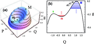
Figure 1: (a) Quasienergy landscape in phase space of a driven Duffing oscillator. The extrema correspond to the high amplitude stable state (M) and the low amplitude stable state (m), while the saddle point (s) denotes an unstable state. (b) Cross-section of the quasienergy potential at $P=0$. Quantum energy levels close to the maximum (M) and minimum (m) of the potential are depicted by blue and red lines, respectively. The unstable saddle point (s) is also indicated.

II.1 Model Hamiltonian

An extensive class of macroscopic physical systems, such as Josephson junctions and nanomechanical oscillators can be modeled by the Duffing oscillator in the presence of a periodic driving force with the system Hamiltonian described by Ser07

$${H}_{S}(t)=\frac{{p}^{2}}{2m}+\frac{1}{2}m\Omega^{2}{x}^{2}-\gamma{x}^{4}+F(t){x}.$$ (1)

Here, parameter $m$ ($\Omega$) describes the mass (frequency) of the oscillator, $\gamma$ gives the nonlinearity of Duffing oscillator, and $F(t)=F_{0}(e^{i\nu t}+e^{-i\nu t})$ describes the periodically driving force with frequency $\nu$. By switching to the rotating frame using the transformation $U(t)=\exp(-i\nu a^{\dagger}at)$, where $a^{\dagger}$ and $a$ are the oscillator raising and lowering operators, and applying the rotating wave approximation (RWA), we obtain a time-independent Hamiltonian

$$H=(\delta\omega+\chi)a^{\dagger}a+\chi(a^{\dagger}a)^{2}+\epsilon(a^{\dagger}+a)\,,$$ (2)

where $\delta\omega=\hbar(\Omega-\nu)$ is the frequency detuning, $\chi=-3\gamma\hbar^{2}/2(m\Omega)^{2}$ is the scaled dimensionless nonlinearity, and $\epsilon=F_{0}\sqrt{{\hbar}/{2m\Omega}}$ is the scaled driving strength. We then introduce the position operator $Q$ and momentum operator $P$ in the rotating frame via

$$Q=\sqrt{\frac{\lambda}{2}}(a^{\dagger}+a),\ \ \ P=i\sqrt{\frac{\lambda}{2}}(a^{\dagger}-a),$$ (3)

which satisfy the commutation relation

$$[Q,P]=i\lambda.$$ (4)

Here, the parameter $\lambda=-\chi/(4\Delta)$ is the dimensionless Planck constant that describes the quantumness of the system, i.e., the value of $\lambda$ increases as the system approaches the quantum regime. Substituting operators $Q$ and $P$ back into the RWA Hamiltonian (2), we obtain

$$H/\Delta=\frac{1}{\lambda}(g+\frac{1}{4})-\frac{1}{2}+\frac{\lambda}{4},$$ (5)

where $g$ is the quasienergy given by

$$g=-(Q^{2}+P^{2}-1)^{2}/4+\sqrt{\beta}Q.$$ (6)

Here, the parameter $\beta=-f^{2}\chi/(2\Delta^{3})$ is the scaled driving strength. Note that Eq. (6) is valid only for the soft nonlinearity $\chi>0$. For the hard nonlinearity $\chi<0$, the quasienergy is given by $g=(Q^{2}+P^{2}-1)^{2}/4-\sqrt{\beta}Q$.

II.2 Renormalized master equation

The characteristic behavior of the driven Duffing system is the bistability manifesting as two stable states: the low-amplitude state (LAS) and the high-amplitude state (HAS). As depicted in Fig. 1(a), these stable states correspond to the extrema in the quasienergy landscape, which are defined as the attractors in the phase space. The unstable state, known as the saddle point, is located on the separatrix, serving as the boundary dividing the basins of the attractors. When damping is present, the system evolves towards the nearby attractor if its initial state lies within the basin of the attractor. However, due to thermal noise, the system does not remain exactly on the attractor, but forms a probability distribution within its basin of attraction. To describe the dissipative dynamics of our system, we employ a Lindblad form master equation

$$\frac{d\rho}{dt}=-i[H,{\rho}]+\frac{\kappa}{2}\{(1+\bar{n}){\cal D}[a]{\rho}+\bar{n}{\cal D}[a^{\dagger}]{\rho}\},$$ (7)

where ${\cal D}[\bullet]$ is the Lindblad operator defined as ${\cal D}[A]{\rho}\equiv 2A{\rho}A^{\dagger}-A^{\dagger}A{\rho}-{\rho}A^{\dagger}A$, $\bar{n}$ is the Bose-Einstein distribution, and $\kappa$ is the damping strength.

To study the quantum dynamics near the bottom of each stable state, we first transform the system to the center of the attractor using the displacement operator

$$D[\alpha]=e^{\alpha a^{\dagger}-\alpha^{*}a}$$ (8)

with parameter $\alpha$ a complex number. By defining the displaced density matrix $\tilde{\rho}=D[\alpha]^{\dagger}\rho D[\alpha]$, we obtain the following master equation

$$\frac{d\tilde{\rho}}{dt} = -i\left[\tilde{H},{\tilde{\rho}}\right]+\frac{\kappa}{2}\{(1+\bar{n}){\cal D}[a]{\tilde{\rho}}+\bar{n}{\cal D}[a^{\dagger}]{\tilde{\rho}}\}$$ (9)

$$+\left[{\tilde{\alpha}}^{*}a-{\tilde{\alpha}}a^{\dagger},\tilde{\rho}\right]\,,$$

with ${\tilde{\alpha}}=[\frac{1}{2}\kappa+i(\delta\omega+\chi+2\chi\alpha|^{2})]\alpha+i\varepsilon.$ By choosing $\alpha$ such that $\tilde{\alpha}=0$, the master equation is simplified into

$$\frac{d\tilde{\rho}}{dt} = -[\tilde{H},{\tilde{\rho}}]+\frac{\kappa}{2}\{(1+\bar{n}){\cal D}[a]{\tilde{\rho}}+\bar{n}{\cal D}[a^{\dagger}]{\tilde{\rho}}\}$$ (10)

with the renormalized Hamiltonian $\tilde{H}$ given by

$$\tilde{H} = (\delta\omega+4\chi|\alpha|^{2})a^{\dagger}a+\chi(a^{\dagger}a)^{2}+\chi({\alpha^{*}}^{2}a^{2}+{\alpha}^{2}{a^{\dagger}}^{2})$$ (11)

$$+2\chi(\alpha{a^{\dagger}}^{2}a+\alpha^{*}{a^{\dagger}}a^{2}).$$

We then introduce the squeezing operator

$$S(\xi)=e^{(\xi^{*}a^{2}-\xi{a^{\dagger}}^{2})/2},$$ (12)

which has the transformation property $S^{\dagger}aS=va+ua^{\dagger}$ with $v=\cosh(|\xi|)$ and $u=-\frac{|\xi|}{\xi}\sinh(|\xi|)$. Bu defining the squeezed density operator $\bar{\rho}=S^{\dagger}\tilde{\rho}S$, we transform the master equation Eq. (10) into the following form

$$\frac{d\bar{\rho}}{dt} = -i[\bar{H},\bar{\rho}]+\frac{\kappa}{2}\{(1+\bar{N}){\cal D}[a]\bar{\rho}+\bar{N}{\cal D}[a^{\dagger}]\bar{\rho}\}$$ (13)

$$+\frac{\kappa}{2}M(2a^{\dagger}\bar{\rho}a^{\dagger}-{a^{\dagger}}^{2}\bar{\rho}-\bar{\rho}{a^{\dagger}}^{2})$$

$$+\frac{\kappa}{2}M^{*}(2a\bar{\rho}a-{a}^{2}\bar{\rho}-\bar{\rho}{a}^{2})$$

$$-i[\bar{\xi}{a^{\dagger}}^{2}+\bar{\xi}^{*}{a}^{2},\bar{\rho}],$$

where $\bar{N}=\bar{n}|v|^{2}+(1+\bar{n})|u|^{2}$ is the effective Bose distribution and $M=uv^{*}(2\bar{n}+1)$ is the squeezing number. The parameter $\bar{\xi}$ in the last term of Eq. (13) is given by

$$\bar{\xi}=[\delta\omega+4\chi|\alpha|^{2}+2\chi(2|u|^{2}+|v|^{2})]v^{*}u+\chi({\alpha^{*}}^{2}u^{2}+\alpha^{2}{v^{*}}^{2}).$$

By setting $\bar{\xi}=0$, the renormalized master equation (13) is further simplified into

$$\frac{d\bar{\rho}}{dt} = -i[\bar{H},\bar{\rho}]+\frac{\kappa}{2}\{(1+\bar{N}){\cal D}[a]\bar{\rho}+\bar{N}{\cal D}[a^{\dagger}]\bar{\rho}\}$$ (14)

$$+\frac{\kappa}{2}M(2a^{\dagger}\bar{\rho}a^{\dagger}-{a^{\dagger}}^{2}\bar{\rho}-\bar{\rho}{a^{\dagger}}^{2})$$

$$+\frac{\kappa}{2}M^{*}(2a\bar{\rho}a-{a}^{2}\bar{\rho}-\bar{\rho}{a}^{2})\,.$$

The final renormalized Hamiltonian $\bar{H}$ becomes

$$\bar{H} = \delta\bar{\omega}a^{\dagger}a+\bar{\chi}(a^{\dagger}a)^{2}$$

$$+2\chi S^{\dagger}(\alpha{a^{\dagger}}^{2}a+\alpha^{*}{a^{\dagger}}a^{2})S+\chi F,$$

with $F=2(|v|^{2}+|u|^{2})(v^{*}u{a^{\dagger}}^{3}a+vu^{*}a^{\dagger}a^{3})+(v^{*}u)^{2}{a^{\dagger}}^{4}+(u^{*}v)^{2}{a}^{4}$. The renormalized detuning $\delta\bar{\omega}$ and nonlinearity $\bar{\chi}$ are given by

$$\left\{\begin{array}[]{lll}\delta\bar{\omega}/\delta\omega&=&(1-4\lambda|\alpha|^{2})(|v|^{2}+|u|^{2})\\ &&-2\lambda(2|uv|^{2}+|u|^{4}+{\alpha^{*}}^{2}uv+\alpha^{2}u^{*}v^{*}),\\ \bar{\chi}/\delta\omega&=&-\lambda(|u|^{4}+|v|^{4}+4|uv|^{2})\end{array}\right.$$ (19)

with the displacement parameter $\alpha$, the squeezing parameters $u$ and $v$ satisfying the following steady equations

$$\left\{\begin{array}[]{lll}&0=&[\frac{\kappa}{2\delta\omega}+i(1-\lambda-2\lambda|\alpha|^{2})]\alpha-i\sqrt{\frac{\beta}{2\lambda}},\\ &0=&[1-4\lambda|\alpha|^{2}-\lambda(4|u|^{2}+2|v|^{2})]v^{*}u\\ &&-\lambda({\alpha^{*}}^{2}u^{2}+\alpha^{2}{v^{*}}^{2}).\end{array}\right.$$ (23)

Here, we have introduced the dimensionless driving strength $\beta=2\lambda(\varepsilon/\delta\omega)^{2}$.

II.3 Orders of perturbative parameters

To perform perturbation calculations for the renormalized Hamiltonian (II.2), we can choose dimensionless Planck constant $\lambda=-\chi/(4\Delta)$ as the natural choice for the perturbation parameter. However, since the displacement parameter $\alpha$ is also a function of $\lambda$, it is subtle to properly organize the perturbative terms according to their respective orders. In fact, the Hamiltonian (II.2) should be written in different forms for different attractors. The stable state of the driven Duffing oscillator can be approximated as a coherent state $|\alpha\rangle$. By applying the variational principle in quantum mechanics, i.e., $\partial_{\alpha}\langle\alpha|H|\alpha\rangle=0$, we obtain two solutions of the steady coherent number: a smaller one $|\alpha_{l}|^{2}\approx\beta/(2\lambda)$ for the LAS and a larger one $|\alpha_{h}|^{2}\approx 1/(2\lambda)$ for the HAS.

For the LAS, we sort the terms in the renormalized Hamiltonian (II.2) as follows

$$\frac{\bar{H}^{l}}{\delta\omega}=h^{l}_{0}+\lambda h^{l}_{\lambda}+\beta h^{l}_{\beta}+\sqrt{\lambda\beta}h^{l}_{\lambda\beta},$$ (24)

with each term given by

$$h^{l}_{0} = (|v|^{2}+|u|^{2})a^{\dagger}a,$$

$$h^{l}_{\lambda} = -2(2|uv|^{2}+|u|^{4})a^{\dagger}a$$

$$-(|u|^{4}+|v|^{4}+4|uv|^{2})(a^{\dagger}a)^{2}-F,$$

$$h^{l}_{\beta} = -\frac{1}{\beta}[{4\lambda|\alpha_{l}|^{2}}(|v|^{2}+|u|^{2})$$

$$+\lambda(2{\alpha^{*}_{l}}^{2}uv+2\alpha^{2}_{l}u^{*}v^{*})]a^{\dagger}a,$$

$$h^{l}_{\lambda\beta} = -2\sqrt{{\lambda}/{\beta}}\ S^{\dagger}(\alpha_{l}{a^{\dagger}}^{2}a+\alpha^{*}_{l}{a^{\dagger}}a^{2})S\,.$$ (25)

Together with Eq. (23), we can now perform perturbative calculations near the bottom of the LAS. Given that the dimensionless driving strength $\beta$ is also small, we consider the sum of the last three terms in the Hamiltonian Eq. (24) as the perturbation term and calculate the desired quantities perturbatively.

For the HAS, as the coherent number $|\alpha_{h}|^{2}\approx 1/(2\lambda)$ can be significantly large for $\lambda\ll 1$, a more careful sorting of the terms in the renormalized Hamiltonian Eq. (II.2) is needed, along with the steady-state condition Eq. (23), to ensure terms of the same order are kept together. We introduce $\gamma=\sqrt{\lambda}$ as the perturbation parameter and rewrite the Hamiltonian as

$$\frac{\bar{H}^{h}}{\delta\omega} = h^{h}_{0}+\gamma h^{h}_{1}+\gamma h^{h}_{2}$$ (26)

with each term given by

$$h^{h}_{0} = [(1-4\lambda|\alpha_{h}|^{2})(|v|^{2}+|u|^{2})$$

$$-2\lambda({\alpha^{*}_{h}}^{2}uv+\alpha_{h}^{2}u^{*}v^{*})]a^{\dagger}a\,,$$

$$h^{h}_{1} = -\sqrt{{\lambda}}\ S^{\dagger}(2\alpha_{h}{a^{\dagger}}^{2}a+2\alpha^{*}_{h}{a^{\dagger}}a^{2}+\alpha_{h}{a^{\dagger}}+\alpha^{*}_{h}a)S\,,$$

$$h^{h}_{2} = -2(2|uv|^{2}+|u|^{4})a^{\dagger}a-(|u|^{4}+|v|^{4}+4|uv|^{2})(a^{\dagger}a)^{2}$$ (27)

$$-F-2(2|u|^{2}+|v|^{2})(v^{*}u{a^{\dagger}}^{2}+u^{*}v{a}^{2})\,.$$

To handle the perturbation orders coherently, we have rearranged the perturbation terms by removing those of order $\lambda$ from the steady condition Eq. (23) and incorporating them into the renormalized Hamiltonian. The coherent number $\alpha_{h}$, $u$ and $v$ for the HAS are now determined by the revised steady condition

$$\left\{\begin{array}[]{lll}&&[\frac{\kappa}{2\delta\omega}+i(1-2\lambda|\alpha_{h}|^{2})]\alpha_{h}-i\sqrt{\frac{\beta}{2\lambda}}=0,\\ &&(1-4\lambda|\alpha_{h}|^{2})v^{*}u-\lambda({\alpha^{*}_{h}}^{2}u^{2}+\alpha_{h}^{2}{v^{*}}^{2})=0.\end{array}\right.$$ (29)

The behavior near the bottom of the LAS is relatively simple and can be modeled using a harmonic oscillator. However, for the HAS, the nonlinear term $\chi(a^{\dagger}a)^{2}\approx\chi|\alpha_{h}|^{2}$ becomes prominent, and the oscillator behaves as a highly squeezed coherent state. In the following sections, we will apply our perturbative method to calculate the crucial quantities related to the HAS of the driven Duffing oscillator, namely the level spacing, averaged position of energy level, and the effective temperature in the vicinity of the HAS attractor.

III Results

III.1 Quantum dynamics of HAS

The quantum dynamics of the driven Duffing oscillator near the HAS attractor exhibit a rich interplay between nonlinearity, quantum fluctuations, and thermal noise. In this section, we discuss the quantum properties of the HAS using the renormalized master equation combined with a refined perturbation theory.

III.1.1 Level Spacing

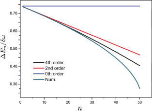
Figure 2: Comparison of perturbation calculations and exact results for energy level spacing. The exact results (lowest curve) for level spacing $\Delta E_{n}=|E_{n+1}-E_{n}|$ are compared with the zeroth-order (constant spacing), the second-order (second highest line, $\gamma^{2}=\lambda$) and the fourth-order (third highest line, $\gamma^{4}=\lambda^{2}$) corrections. Excellent agreement is observed for low level numbers near the potential well bottom, while higher-order corrections are required for large $n$. Parameters: $\lambda=0.016$ and $\beta=4/75$.

The nonlinearity term $\chi(a^{\dagger}a)^{2}$ in the Hamiltonian, having an opposite sign to $\delta\omega$, results in a decrease in the level spacing $\Delta E_{n}=|E_{n+1}-E_{n}|$ as we approach the saddle point, as illustrated in Fig. 1(b). One can calculate the level spacings with standard perturbation theory by treating the sum of $\gamma h_{1}^{h}$ and $\gamma h_{2}^{h}$ in Eq. (26) as one perturbation term. However, it becomes a challenge to control the accuracy of the level spacings by the perturbative parameter. We find it necessary to distinguish between these two perturbative terms in the perturbation calculations to accurately determine the level spacing. To address this, we have developed a double perturbation theory framework that is particularly suited for the HAS Hamiltonian containing second-order small terms, see the details in Appendix A,

In Fig. 2, we compare our perturbation calculations with the exact numerical results obtained by diagonalizing the original Hamiltonian Eq. (2), which shows an excellent agreement for energy levels near the bottom of the potential well. Under the zeroth-order perturbation approximation, the energy level spacing remains constant across all levels, similar to that of harmonic oscillators. The second-order and fourth-order corrections correspond to accuracies up to $\gamma^{2}=\lambda$ and $\gamma^{4}=\lambda^{2}$, respectively. Higher-order perturbation calculations become necessary for levels farther from the bottom.

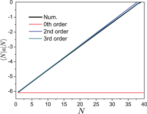
Figure 3: Average position of energy levels. Average position $\langle N|a|N\rangle$ of the energy level $N$, illustrating the shifts due to quantum fluctuations. Under the harmonic approximation, $\langle N|a|N\rangle$ is a constant for every level (lowest line). Considering higher-order corrections, we observe changes in $\langle N|a|N\rangle$ with levels. Comparing with the second order perturbation result (highest line), the third order result (second highest line) already align well with the exact one (the bold line).

III.1.2 Averaged level position

We denote the eigenstate of the renormalized Hamiltonian $\bar{H}$ as $|n^{\prime}\rangle$ that is generally a superposition of harmonic oscillator eigenstates $|n^{\prime}\rangle=|n\rangle+\sum_{k\neq n}\xi_{kn}|k\rangle$, where the superposition coefficients $\xi_{kn}$ are provided in the Appendix A. The eigenstate $|N\rangle$ of the original Hamiltonian (2) is related to that of the renormalized Hamiltonian (II.2) via the relationship $|N\rangle=DS|n^{\prime}\rangle$. The matrix element $\langle N|a|M\rangle$ for different levels $|N\rangle$ and $|M\rangle$ is then given by

$$\langle N|a|M\rangle = \langle n^{\prime}|S^{\dagger}D^{\dagger}aDS|m^{\prime}\rangle$$

$$= \langle n^{\prime}|(va+u^{\dagger}+\alpha)|m^{\prime}\rangle$$

$$= v\langle n^{\prime}|a|m^{\prime}\rangle+u\langle m^{\prime}|a|n^{\prime}\rangle^{*}+\alpha\langle n^{\prime}|m^{\prime}\rangle\,.$$

The matrix element $\langle N|a|N\rangle$ provides insight into the average position of each level in the phase space. Under the harmonic approximation ($\xi_{kn}=0$), $\langle N|a|N\rangle$ is a constant $\alpha$ for all levels. However, considering higher-order corrections, the average position $\langle N|a|N\rangle$ changes with energy level, as depicted in Fig. 3. The perturbation calculations agree well with numerical results.

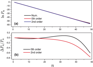
Figure 4: Comparison of stationary probability distributions. (a) Comparison of the stationary probability distribution obtained through perturbation theory to zeroth order (red line), second order (blue lines) and exact numerical simulations (black line). (b) Relative error $\Delta p_{n}/p_{n}$ in the stationary distribution obtained from perturbation theory compared to numerical results. The discrepancy increases for higher levels but remains less than 1.

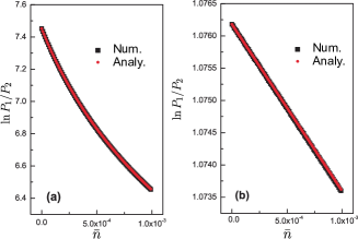
Figure 5: Ratio of probabilities for the lowest levels in (a) the LAS and (b) HAS, plotted as a function of the Bose distribution $\bar{n}$. The agreement between the analytical results (black square dots) and the exact numerical results (red circle dots) is excellent.

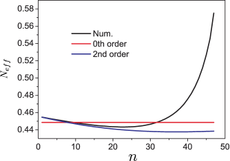
Figure 6: Effective temperature of energy levels. The stationary probability distributions $N_{eff}(n)$ of level $|n\rangle$ obtained through perturbation theory to zeroth order (red line) and second order (blue lines) are compared with the exact numerical simulations (black line). The zero-order effective temperature term gives a constant effective temperature. The second order results in changes in $N_{eff}(n)$, which is quite accurate for levels near the bottom.

III.1.3 Effective temperature

Next, we calculate the stationary distribution over the levels of the HAS and the effective temperature near the bottom. It is important to note that the annihilation operator $a$ is for the Fock state $|N\rangle$, which decreases the Fock state from a higher level to the next lower level $a|N\rangle=\sqrt{N}|N-1\rangle$. However, in our case, the eigenstate of quasienergy $|n\rangle$ is the superposition of the Fock state $|N\rangle$. As a result, the annihilation operator $a$ can either decrease or increase the state $|n\rangle$ even at zero temperature.

Under the assumption of weak damping ($\kappa\ll E_{n}-E_{n+1}$), the off-diagonal matrix elements on the state $|n\rangle$ are very small. Thus, we can only keep the diagonal elements. Here, we assume that the stationary density matrix is diagonal and denote the diagonal terms $p_{n^{\prime}}=\langle n^{\prime}|\rho|n^{\prime}\rangle$. The master equation (II.2) can be simplified into a balance equation Dyk06

$$\frac{dp_{n^{\prime}}}{dt}=\kappa\sum_{m^{\prime}}(W_{n^{\prime},m^{\prime}}p_{m^{\prime}}-W_{m^{\prime},n^{\prime}}p_{n^{\prime}}),$$ (31)

where the transition rate from level $|m^{\prime}\rangle$ to level $|n^{\prime}\rangle$ ($m^{\prime}\neq n^{\prime}$) is given by

$$W_{n^{\prime},m^{\prime}} = M\langle m^{\prime}|a|n^{\prime}\rangle^{*}\langle n^{\prime}|a|m^{\prime}\rangle^{*}+M^{*}\langle m^{\prime}|a|n^{\prime}\rangle\langle n^{\prime}|a|m^{\prime}\rangle$$ (32)

$$+(1+\bar{N})|\langle n^{\prime}|a|m^{\prime}\rangle|^{2}+\bar{N}|\langle m^{\prime}|a|n^{\prime}\rangle|^{2}.$$

One can prove that the transition rate $W_{n^{\prime},m^{\prime}}$ for $n^{\prime}\neq m^{\prime}$ is equal to $|\langle N|a|M\rangle|^{2}$ calculated above in Eq. (III.1.2) .

As can be seen from the above rate equation, even at zero temperature, the oscillator can make transitions to both lower and higher energy levels. In Fig. 4, we compare the stationary distribution obtained using our double perturbation theory with exact numerical results. To the lowest order, all superposition coefficients are zero. To the first order of $\sqrt{\lambda}$ (i.e., $\xi_{kn}=\sqrt{\lambda}\xi^{(1)}_{kn}$), there is no correction to the stationary distribution $p_{n^{\prime}}$. Then, to the second order (i.e., $\xi_{kn}=\sqrt{\lambda}\xi^{(1)}_{kn}+\lambda\xi^{(2)}_{kn}$), we solve the balance equation (31) accordingly. Fig.4 (b) illustrates the relative error $\Delta p_{n}/p_{n}$ in comparison to the exact numerical results, which shows that the discrepancy for low levels is mitigated by high-order perturbative calculations.

In the vicinity of the bottom, we can apply the harmonic approximation ($\xi_{kn}=0$). Under this approximation, the ratio of probabilities over adjacent levels is

$$\frac{p_{n^{\prime}+1}}{p_{n^{\prime}}} = \frac{W_{n^{\prime}+1,n^{\prime}}}{W_{n^{\prime},n^{\prime}+1}}=\frac{\bar{N}}{1+\bar{N}}$$ (33)

$$= \frac{\bar{n}|v|^{2}+(1+\bar{n})|u|^{2}}{1+\bar{n}|v|^{2}+(1+\bar{n})|u|^{2}}.$$

We verify the relationship between $\ln(p_{1}/p_{2})$ and the Bose distribution $\bar{n}$ in Fig. 5. The agreement between the analytical results from Eq. (33) and the exact numerical one is excellent.

For high levels, we can define the level-dependent effective temperature via

$$N_{eff}(n)\equiv p_{n+1}/(p_{n}-p_{n+1})$$

for level $|n\rangle$. Fig. 6 illustrates how $N_{eff}$ varies from the lowest to higher levels. The zero-order term yields a constant effective temperature. When we include the correction to the order of $\lambda$, the correction leads to changes in $N_{eff}$ showing a good agreement with the numerical results for levels near the bottom.

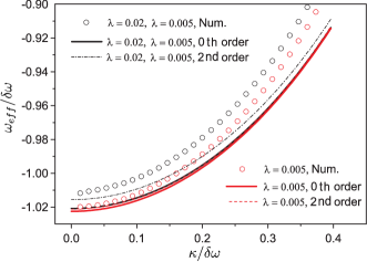
Figure 7: Relationship between effective frequency $\omega_{eff}=\Delta E_{1}$ and damping strength $\kappa$. Results obtained from the emission spectrum method (circles), cf. Eq. (34), are compared with those from our perturbation theory (solid and dashed lines).

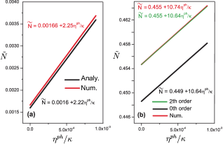
Figure 8: Renormalized effective Bose distribution $\tilde{N}$ due to dephasing effects for (a) the LAS and (b) the HAS. We compare the theoretical predictions from Eq. (36) with the exact numerical results and extract the linear relationships.

III.2 Strong Damping and Dephasing

In this section, we explore the dynamics and stationary state of the system under conditions of strong damping and dephasing, which can significantly alter the behavior predicted by the weak damping approximation.

III.2.1 Strong damping

In the regime of strong damping, the harmonic approximation, which leads to the level spacing $\Delta E_{n}$ that is independent of damping, is no longer valid. Instead, the level spacing undergoes slight renormalization for strong damping. Such effect can be observed through the emission spectrum $S(\omega)$, representing the spectral density of photons emitted by the driven resonator, is given by

$$S(\omega)=2\operatorname{Re}\int_{0}^{\infty}e^{-i\omega t}\text{Tr}[a^{\dagger}e^{\mathcal{L}t}(a\rho_{\text{st}})]{\rm d}t\,.$$ (34)

Our method inherently incorporates damping effects into the calculation of $\Delta E_{n}$. For finite damping, the squeezing parameters $u$ and $v$ are complex numbers, determined by the steady-state conditions given in Eq. (29). Substituting them into Eq. (26), we obtain the effective frequency $\omega_{eff}=\Delta E_{1}$. In Fig. 7, we compare the results obtained through the emission spectrum Eq. (34) with those from our perturbation theory, demonstrating satisfactory consistency. The minor discrepancy arises primarily from higher-level spacings $\Delta E_{n}(n>1)$, which are typically smaller than the first-level spacing $\Delta E_{1}$. For more accurate results, the average of all level spacings should be considered in the calculations.

III.2.2 Dephasing

To incorporate dephasing, we introduce the dephasing term $\eta^{ph}{\cal D}[a^{\dagger}a]{\rho}$ into the master equation (7). For convenience, we define a generalized Lindblad operator ${\cal L}[A;B]\rho\equiv 2A\rho B-BA\rho-\rho AB$. In the spirit of the rotating wave approximation, we obtain the renormalized master equation for the displaced and squeezed density ioperator $\bar{\rho}=S^{\dagger}D^{\dagger}{\rho}DS$ (see detailed derivation in Appendix B)

$$\frac{d\bar{\rho}}{dt} = -i[\bar{H},\bar{\rho}]+\frac{\kappa}{2}\{(1+\tilde{N}){\cal D}[a]\bar{\rho}+\tilde{N}{\cal D}[a^{\dagger}]\bar{\rho}\}$$ (35)

$$+\frac{\kappa}{2}M{\cal L}[a^{\dagger};a^{\dagger}]{\bar{\rho}}+\frac{\kappa}{2}M^{*}{\cal L}[a;a]{\bar{\rho}}$$

$$+\eta^{ph}(|v|^{2}+|u|^{2})^{2}{\cal D}[a^{\dagger}a]{\bar{\rho}}$$

$$+\eta^{ph}|uv|^{2}({\cal D}[{a^{\dagger}}^{2}]{\bar{\rho}}+{\cal D}[a^{2}]{\bar{\rho}}),$$

where the renormalized Bose distribution, affected by dephasing, is given by:

$$\tilde{N} = \bar{N}+\frac{\eta^{ph}}{\kappa}|\alpha^{*}u+\alpha v^{*}|^{2}$$ (36)

$$= |u|^{2}+\bar{n}(|u|^{2}+|v|^{2})+\frac{\eta^{ph}}{\kappa}|\alpha^{*}u+\alpha v^{*}|^{2}\,.$$

We verify our predictions for renormalized Bose distribution by comparing them with exact numerical simulations according to the probabilities over the two lowest levels, specifically $\tilde{N}=p_{2}/(p_{1}-p_{2})$. In Fig. 8, we plot and extract the renormalized Bose distribution as a function of the dephasing, which demonstrates an excellent agreement between the numerical results and the analytical predictions given by Eq. (36) for both LAS and HAS.

IV Conclusions

In this work, we have investigated the quantum dissipative dynamics of a driven Duffing oscillator near the bottoms of its stable states. We elucidated the intricate interplay between the nonlinearity, quantum fluctuations, and the influence of an external driving field. We formulated an effective quantum master equation that encompasses quantum and thermal fluctuations, strong damping, and dephasing within a unified framework. We have developed a refined perturbation theory to analyze the quantum dynamics near both the LAS and the HAS of the Duffing oscillator. While the LAS behavior can be approximated using a harmonic oscillator model, the HAS exhibits more complex behavior due to the significant nonlinear terms. Due to quantum fluctuations, even at zero temperature, higher energy levels near the bottom of the potential well are excited. We calculated the level spacing and effective temperature near the bottom of the HAS and compare them with numerical simulations, demonstrating the accuracy and utility of our proposed approach.

We also investigated the effects of strong damping and dephasing on the system’s dynamics. We showed that the level spacing undergoes slight renormalization for strong damping, which can be observed through the emission spectrum. We derived the renormalized quantum master equation and analyzed the system’s behavior affected by dephasing. Our work provides new insights into the quantum dynamics of driven Duffing oscillators, particularly near their stable states, and offers a theoretical framework that can be applied to related quantum systems under strong damping and dephasing conditions.

ACKNOWLEDGMENTS

This work was supported by Natural Science Foundation of China (Grant No. 12475025).

AUTHOR DECLARATIONS

Conflict of interest

The authors have no conflicts to disclose.

Author contributions

The two authors contributed equally to this work.

DATA AVAILABILITY

The data that support the findings of this study are available within the article.

Appendix A Double Perturbation Theory

To effectively address Hamiltonians containing second-order perturbation terms, exemplified by the HAS in the driven Duffing oscillator, we develop a framework for double perturbation theory. This theory is specifically designed for systems where treating the second-order terms independently is essential for maintaining computational precision and obtaining physically meaningful results. Consider a Hamiltonian of the general form:

$${H}=H_{0}+\gamma H_{1}+\gamma^{2}H_{2},$$ (37)

where $\gamma$ is a small parameter. In conventional perturbation theory, the terms $\gamma H_{1}+\gamma^{2}H_{2}$ are often treated as a single perturbation term. However, for the HAS of the driven Duffing system, this approach does not yield results with the necessary accuracy. Therefore, we introduce the concept of double perturbation theory, where the terms are handled separately.

The eigenvalues and eigenstates of $H_{0}$ are denoted as $\epsilon^{(0)}_{n}$ and $|\psi^{(0)}_{n}\rangle$ respectively, satisfying $H_{0}|\psi^{(0)}_{n}\rangle=\epsilon^{(0)}_{n}|\psi^{(0)}_{n}\rangle$. The exact eigenvalues and eigenstates of $H$ are denoted as $\epsilon_{n}$ and $|\psi_{n}\rangle$, which can be expanded in powers of $\gamma$ as:

$$\epsilon_{n} = \epsilon^{(0)}_{n}+\gamma\epsilon^{(1)}_{n}+\gamma^{2}\epsilon^{(2)}_{n}+\gamma^{3}\epsilon^{(3)}_{n}+\gamma^{4}\epsilon^{(4)}_{n}+o(\gamma^{5}),$$

$$|\psi_{n}\rangle = |\psi^{(0)}_{n}\rangle+\gamma\sum_{k\neq n}\xi^{(1)}_{kn}|\psi^{(0)}_{k}\rangle+\gamma^{2}\sum_{l\neq n}\xi^{(2)}_{ln}|\psi^{(0)}_{l}\rangle$$

$$+\gamma^{3}\sum_{m\neq n}\xi^{(3)}_{mn}|\psi^{(0)}_{m}\rangle+\gamma^{4}\sum_{p\neq n}\xi^{(4)}_{pn}|\psi^{(0)}_{p}\rangle+o(\gamma^{5}).$$

From the eigenvalue equation $H|\psi_{n}\rangle=\epsilon_{n}|\psi_{n}\rangle$, we can derive the perturbative results order by order:

1) to the order of $\gamma^{0}=1$: $H_{0}|\psi^{(0)}_{n}\rangle=\epsilon^{(0)}_{n}|\psi^{(0)}_{n}\rangle$;

2) to the order of $\gamma$:

$$\gamma(\sum_{k\neq n}\epsilon^{(0)}_{k}\xi^{(1)}_{kn}|\psi^{(0)}_{k}\rangle+H_{1}|\psi^{(0)}_{n}\rangle)$$ (39)

$$= \gamma(\sum_{k\neq n}\epsilon^{(0)}_{n}\xi^{(1)}_{kn}|\psi^{(0)}_{k}\rangle+\epsilon^{(1)}_{n}|\psi^{(0)}_{n}\rangle)\,,$$

which gives us the perturbative result to the first order

$$\epsilon^{(1)}_{n} = \langle\psi^{(0)}_{n}|H_{1}|\psi^{(0)}_{n}\rangle,$$

$$\xi^{(1)}_{kn} = \frac{1}{\epsilon^{(0)}_{n}-\epsilon^{(0)}_{k}}\langle\psi^{(0)}_{k}|H_{1}|\psi^{(0)}_{n}\rangle;$$ (40)

3) to the order of $\gamma^{2}$:

$$\gamma^{2}(\sum_{l\neq n}\epsilon^{(0)}_{l}\xi^{(2)}_{ln}|\psi^{(0)}_{l}\rangle+\sum_{k\neq n}\xi^{(1)}_{kn}H_{1}|\psi^{(0)}_{k}\rangle+H_{2}|\psi^{(0)}_{n}\rangle)$$

$$=\gamma^{2}(\sum_{l\neq n}\epsilon^{(0)}_{n}\xi^{(2)}_{ln}|\psi^{(0)}_{l}\rangle+\sum_{k\neq n}\xi^{(1)}_{kn}\epsilon^{(1)}_{n}|\psi^{(0)}_{k}\rangle+\epsilon^{(2)}_{n}|\psi^{(0)}_{n}\rangle),$$

which gives us the second order perturbative result:

$$\epsilon^{(2)}_{n} = \sum_{k\neq n}\langle\psi^{(0)}_{n}|H_{1}|\psi^{(0)}_{k}\rangle\xi^{(1)}_{kn}+\langle\psi^{(0)}_{n}|H_{2}|\psi^{(0)}_{n}\rangle,$$

$$\xi^{(2)}_{ln} = \frac{1}{\epsilon^{(0)}_{n}-\epsilon^{(0)}_{l}}(\sum_{k\neq n}\langle\psi^{(0)}_{l}|H_{1}|\psi^{(0)}_{k}\rangle\xi^{(1)}_{kn}+\langle\psi^{(0)}_{l}|H_{2}|\psi^{(0)}_{n}\rangle$$ (42)

$$-\epsilon^{(1)}_{n}\xi^{(1)}_{ln});$$

4) to the order of $\gamma^{3}$:

$$\gamma^{3}(\sum_{m\neq n}\epsilon^{(0)}_{m}\xi^{(3)}_{mn}|\psi^{(0)}_{m}\rangle+\sum_{l\neq n}\xi^{(2)}_{ln}H_{1}|\psi^{(0)}_{l}\rangle$$ (43)

$$+\sum_{k\neq n}\xi^{(1)}_{kn}H_{2}|\psi^{(0)}_{k}\rangle)$$

$$= \gamma^{3}(\sum_{m\neq n}\epsilon^{(0)}_{n}\xi^{(3)}_{mn}|\psi^{(0)}_{m}\rangle+\sum_{l\neq n}\epsilon^{(1)}_{n}\xi^{(2)}_{ln}|\psi^{(0)}_{l}\rangle$$

$$+\sum_{k\neq n}\xi^{(1)}_{kn}\epsilon^{(2)}_{n}|\psi^{(0)}_{k}\rangle+\epsilon^{(3)}_{n}|\psi^{(0)}_{n}\rangle),$$

which gives us the perturbative result to the third order:

$$\epsilon^{(3)}_{n} = \sum_{l\neq n}(\langle\psi^{(0)}_{n}|H_{1}|\psi^{(0)}_{l}\rangle\xi^{(2)}_{ln}+\langle\psi^{(0)}_{n}|H_{2}|\psi^{(0)}_{l}\rangle\xi^{(1)}_{ln})\,,$$

$$\xi^{(3)}_{mn} = \frac{1}{\epsilon^{(0)}_{n}-\epsilon^{(0)}_{m}}[\sum_{l\neq n}(\langle\psi^{(0)}_{m}|H_{1}|\psi^{(0)}_{l}\rangle\xi^{(2)}_{ln}$$ (44)

$$+\langle\psi^{(0)}_{m}|H_{2}|\psi^{(0)}_{l}\rangle\xi^{(1)}_{ln})-\epsilon^{(1)}_{n}\xi^{(2)}_{mn}-\epsilon^{(2)}_{n}\xi^{(1)}_{mn}];$$

5) to the order of $\gamma^{4}$:

$$\gamma^{4}(\sum_{p\neq n}\epsilon^{(0)}_{p}\xi^{(4)}_{pn}|\psi^{(0)}_{p}\rangle+\sum_{m\neq n}\xi^{(3)}_{mn}H_{1}|\psi^{(0)}_{m}\rangle+\sum_{l\neq n}\xi^{(2)}_{ln}H_{2}|\psi^{(0)}_{l}\rangle)$$

$$=\gamma^{4}[\sum_{m\neq n}(\epsilon^{(0)}_{n}\xi^{(4)}_{mn}+\epsilon^{(1)}_{n}\xi^{(3)}_{mn}+\xi^{(2)}_{mn}\epsilon^{(2)}_{n}+\xi^{(1)}_{mn}\epsilon^{(3)}_{n})|\psi^{(0)}_{m}\rangle$$

$$+\epsilon^{(4)}_{n}|\psi^{(0)}_{n}\rangle],$$ (45)

which gives us the fourth order perturbative result:

$$\epsilon^{(4)}_{n} = \sum_{l\neq n}(\langle\psi^{(0)}_{n}|H_{1}|\psi^{(0)}_{l}\rangle\xi^{(3)}_{ln}+\langle\psi^{(0)}_{n}|H_{2}|\psi^{(0)}_{l}\rangle\xi^{(2)}_{ln}),$$

$$\xi^{(4)}_{pn} = \frac{1}{\epsilon^{(0)}_{n}-\epsilon^{(0)}_{p}}[\sum_{l\neq n}(\langle\psi^{(0)}_{p}|H_{1}|\psi^{(0)}_{l}\rangle\xi^{(3)}_{ln}+\langle\psi^{(0)}_{p}|H_{2}|\psi^{(0)}_{l}\rangle\xi^{(2)}_{ln})$$ (46)

$$-\epsilon^{(1)}_{n}\xi^{(3)}_{pn}-\epsilon^{(2)}_{n}\xi^{(2)}_{pn}-\epsilon^{(3)}_{n}\xi^{(1)}_{pn}].$$

Similar expressions can be derived for higher-order corrections.

For the high-amplitude state of the driven Duffing oscillator, the perturbative Hamiltonian is given by Eq. (26),

$$\frac{\bar{H}^{h}}{\delta\omega} = h^{h}_{0}+\gamma h^{h}_{1}+\gamma h^{h}_{2},$$

where the order parameter $\gamma$ is $\sqrt{\lambda}$. The zeroth-order Hamiltonian

$$h^{h}_{0} = [(1-4\lambda|\alpha_{h}|^{2})(|v|^{2}+|u|^{2})$$ (48)

$$-2\lambda({\alpha^{*}_{h}}^{2}uv+\alpha_{h}^{2}u^{*}v^{*})]a^{\dagger}a,$$

corresponds to a harmonic oscillator, and the eigenstates $|\psi^{(0)}_{k}\rangle$ are simply the harmonic oscillator states $|k\rangle$ with eigenvalues:

$$\epsilon^{(0)}_{k} = k[(1-4\lambda|\alpha_{h}|^{2})(|v|^{2}+|u|^{2})$$ (49)

$$-2\lambda({\alpha^{*}_{h}}^{2}uv+\alpha_{h}^{2}u^{*}v^{*})].$$

By calculating the matrix elements $\langle l|h^{h}_{1}|k\rangle$ and $\langle l|h^{h}_{2}|k\rangle$,

$$\langle l|h^{h}_{1}|k\rangle = -2\sqrt{\lambda k}[\alpha_{h}|v|^{2}u^{*}(2k-1)+\alpha_{h}|u|^{2}u^{*}(k+1)+\alpha_{h}^{*}v|u|^{2}(2k+1)+\alpha_{h}^{*}v|v|^{2}(k-1)+(\alpha_{h}^{*}v+\alpha_{h}u^{*})/2]\delta_{l,k-1}$$

$$-2\sqrt{\lambda(k+1)}[\alpha_{h}|u|^{2}v^{*}(2k+3)+\alpha_{h}|v|^{2}v^{*}k+\alpha_{h}^{*}u|v|^{2}(2k+1)+\alpha_{h}^{*}u|u|^{2}(k+2)+(\alpha_{h}^{*}u+\alpha_{h}v^{*})/2]\delta_{l,k+1}$$

$$-2u^{*}v\sqrt{\lambda k(k-1)(k-2)}(\alpha_{h}^{*}v+\alpha_{h}u^{*})\delta_{l,k-3}-2v^{*}u\sqrt{\lambda(k+1)(k+2)(k+3)}(\alpha_{h}^{*}u+\alpha_{h}v^{*})\delta_{l,k+3},$$

$$\langle l|h^{h}_{2}|k\rangle = -[2(2|uv|^{2}+|u|^{4})k+(|u|^{4}+|v|^{4}+4|uv|^{2})k^{2}]\delta_{l,k}$$ (50)

$$-2u^{*}v\sqrt{k(k-1)}[k|u|^{2}+(k-1)|v|^{2}]\delta_{l,k-2}-2v^{*}u\sqrt{(k+1)(k+2)}[(k+2)|u|^{2}+(k+1)|v|^{2}]\delta_{l,k+2}$$

$$-(u^{*}v)^{2}\sqrt{k(k-1)(k-2)(k-3)}\delta_{l,k-4}-(v^{*}u)^{2}\sqrt{(k+1)(k+2)(k+3)(k+4)}\delta_{l,k+4},$$

we can apply the double perturbation theory to obtain the desired perturbative results, such as level spacing and effective temperature, for the high-amplitude state as detailed in the main text.

Appendix B Dephasing

This section presents the derivation of Eq. (35) in the main text. To incorporate dephasing, we introduce the dephasing term $\eta^{ph}{\cal D}[a^{\dagger}a]{\rho}$ into the master equation. For convenience, we define a generalized Lindblad operator ${\cal L}[A;B]\rho\equiv 2A\rho B-BA\rho-\rho AB$, which satisfies

$${\cal D}[A]{\rho}={\cal L}[A;A^{\dagger}]\rho,$$

$${\cal D}[A+B]{\rho}={\cal D}[A]{\rho}+{\cal D}[B]{\rho}+{\cal L}[A;B^{\dagger}]\rho+{\cal L}[B;A^{\dagger}]\rho,$$

$${\cal L}[A;B+C]\rho={\cal L}[A;B]\rho+{\cal L}[A;C]\rho,$$

$${\cal L}[A+B;C]\rho={\cal L}[A;C]\rho+{\cal L}[B;C]\rho,$$

$$({\cal L}[A;B]\rho)^{\dagger}={\cal L}[B^{\dagger};A^{\dagger}]\rho.$$ (51)

Utilizing these properties, we derive the transformed dephasing term under the action of the displacement and squeezing operators:

$$S^{\dagger}D^{\dagger}({\cal D}[a^{\dagger}a]{\rho})DS$$

$$=(|v|^{2}+|u|^{2})^{2}{\cal D}[a^{\dagger}a]{\bar{\rho}}\ +|\alpha^{*}u+\alpha v^{*}|^{2}({\cal D}[a^{\dagger}]{\bar{\rho}}$$

$$+{\cal D}[a]{\bar{\rho}})+|uv|^{2}({\cal D}[{a^{\dagger}}^{2}]{\bar{\rho}}+{\cal D}[a^{2}]{\bar{\rho}})+{\cal L}\bar{\rho}+({\cal L}\bar{\rho})^{\dagger}.$$ (52)

The term ${\cal L}\bar{\rho}$ includes various higher-order terms:

$${\cal L}\bar{\rho} = |uv|^{2}{\cal L}[{a^{\dagger}}^{2};{a^{\dagger}}^{2}]{\bar{\rho}}+|\alpha^{*}u+\alpha v^{*}|^{2}{\cal L}[{a^{\dagger}};{a^{\dagger}}]{\bar{\rho}}+v^{*}u(\alpha^{*}u+\alpha v^{*}){\cal L}[{a^{\dagger}}^{2};{a^{\dagger}}]{\bar{\rho}}+vu^{*}(\alpha u^{*}+\alpha^{*}v){\cal L}[a;a^{2}]{\bar{\rho}}$$

$$+v^{*}u(\alpha u^{*}+\alpha^{*}v){\cal L}[a;{a^{\dagger}}^{2}]{\bar{\rho}}+vu^{*}(\alpha^{*}u+\alpha v^{*}){\cal L}[a^{2};a^{\dagger}]{\bar{\rho}}+(|v|^{2}+|u|^{2})\{v^{*}u{\cal L}[a^{\dagger}a;{a^{\dagger}}^{2}]{\bar{\rho}}+vu^{*}{\cal L}[a^{\dagger}a;a^{2}]{\bar{\rho}}$$

$$+(\alpha^{*}u+\alpha v^{*}){\cal L}[a^{\dagger};a^{\dagger}a]{\bar{\rho}}+(\alpha u^{*}+\alpha^{*}v){\cal L}[a;a^{\dagger}a]{\bar{\rho}}\}.$$

In the spirit of the rotating wave approximation, we neglect the terms ${\cal L}\bar{\rho}$ and $({\cal L}\bar{\rho})^{\dagger}$ in Eq. (B). Adding the dephasing term to the renormalized master equation, we obtain:

$$\frac{d\bar{\rho}}{dt} = -i[\bar{H},\bar{\rho}]+\frac{\kappa}{2}\{(1+\tilde{N}){\cal D}[a]\bar{\rho}+\tilde{N}{\cal D}[a^{\dagger}]\bar{\rho}\}+\frac{\kappa}{2}M{\cal L}[a^{\dagger};a^{\dagger}]{\bar{\rho}}+\frac{\kappa}{2}M^{*}{\cal L}[a;a]{\bar{\rho}}$$ (54)

$$+\eta^{ph}(|v|^{2}+|u|^{2})^{2}{\cal D}[a^{\dagger}a]{\bar{\rho}}+\eta^{ph}|uv|^{2}({\cal D}[{a^{\dagger}}^{2}]{\bar{\rho}}+{\cal D}[a^{2}]{\bar{\rho}}),$$

where the renormalized Bose distribution, affected by dephasing, is given by:

$$\tilde{N} = \bar{N}+\frac{\eta^{ph}}{\kappa}|\alpha^{*}u+\alpha v^{*}|^{2}$$ (55)

$$= |u|^{2}+\bar{n}(|u|^{2}+|v|^{2})+\frac{\eta^{ph}}{\kappa}|\alpha^{*}u+\alpha v^{*}|^{2}\,.$$

References

- (1) G. Duffing, Erzwungene Schwingungen bei veränderlicher Eigenfrequenz und ihre technische Bedeutung, Ingenieur-Archiv 8, 445 (1918).
- (2) M. I. Dykman, Fluctuating nonlinear oscillators: from nanomechanics to quantum superconducting circuits, Oxford University Press, 2012.
- (3) A. N. Cleland and M. L. Roukes, Noise processes in nanomechanical resonators, J. App. Phys., 92, 2758 (2002).
- (4) R. Lifshitz and M. C. Cross, Nonlinear dynamics of nanomechanical and micromechanical resonators, Wiley Meinheim Press, 2008.
- (5) M. Poot and H. S. J. van der Zant, Mechanical systems in the quantum regime, Phys. Rep., 511, 273 (2012).
- (6) J. Choi, H. Hwang, and E. Kim, Measurement-induced bistability in the excited state of a transmon, Phys. Rev. Appl. 22, 054069 (2024).
- (7) T. K. Mavrogordatos, G. Tancredi, M. Elliott, M. J. Peterer, A. Patterson, J. Rahamim, P. J. Leek, E. Ginossar, and M. H. Szymańska, Simultaneous bistability of a qubit and resonator in circuit quantum electrodynamics, Phys. Rev. Lett. 118, 040402 (2017).
- (8) M. Boissonneault, J. M. Gambetta, and A. Blais, Improved superconducting qubit readout by qubit-induced nonlinearities, Phys. Rev. Lett. 105, 100504 (2010).
- (9) P. Del’Haye, A. Schliesser, O. Arcizet, T. Wilken, R. Holzwarth, and T. J. Kippenberg, Optical Frequency Comb Generation from a Monolithic Microresonator, Nature (London) 450, 1214 (2007).
- (10) T. J. Kippenberg, R. Holzwarth, and S. A. Diddams, Microresonator-Based Optical Frequency Combs, Science 332, 555 (2011).
- (11) P. D. Drummond and M. Hillery, The quantum theory of nonlinear optics, Cambridge University Press, 2014.
- (12) E. Bolandhemmat and F. Kheirandish, Quantum dynamics of a driven parametric oscillator in a Kerr medium, Sci. Rep., 13, 9056 (2023).
- (13) F. Hellbach, D. De Bernardis, M. Saur, I. Carusotto, W. Belzig, and G. Rastelli, Nonlinearity-induced symmetry breaking in a system of two parametrically driven Kerr-Duffing oscillators, arXiv:2405.01377 (2024).
- (14) E. Buks and B. Yurke, Mass detection with a nonlinear nanomechanical resonator, Phys. Rev. E 74, 046619 (2006).
- (15) R. Almog, S. Zaitsev, O. Shtempluck, and E. Buks, Noise squeezing in a nanomechanical Duffing resonator, Phys. Rev. Lett. 98, 078103 (2007).
- (16) J. S. Ochs, D. K. J. Bone, G. Rastelli, M. Seitner, W. Belzig , M. I. Dykman , and E. M. Weig, Frequency Comb from a Single Driven Nonlinear Nanomechanical Mode, Phys. Rev. X 12, 041019 (2022).
- (17) A. Bachtold, J. Moser, and M. I. Dykman, Mesoscopic physics of nanomechanical systems, Rev. Mod. Phys. 94, 045005 (2022).
- (18) R. Artuso and L. Rebuzzini, Effects of a nonlinear perturbation on dynamical tunneling in cold atoms, Phys. Rev. E 68, 036221 (2003).
- (19) H. Gothe, T. Valenzuela, M. Cristiani, and J. Eschner, Optical bistability and nonlinear dynamics by saturation of cold Yb atoms in a cavity, Phys. Rev. A 99, 013849 (2019).
- (20) V. Parigi, E. Bimbard, J. Stanojevic, A. J. Hilliard, F. Nogrette, R. Tualle-Brouri, A. Ourjoumtsev, and P. Grangier, Observation and Measurement of Interaction-Induced Dispersive Optical Nonlinearities in an Ensemble of Cold Rydberg Atoms, Phys. Rev. Lett. 109, 233602 (2012)
- (21) J. S. Aldridge and A. N. Cleland, Noise-enabled precision measurement of a Duffing nanomechanical resonator, Phys. Rev. Lett. 94, 156403 (2005).
- (22) I. Siddiqi, R. Vijay, F. Pierre, C. M. Wilson, M. Metcalfe, C. Rigetti, L. Frunzio, and M. H. Devoret, RF-driven Josephson bifurcation amplifier for quantum measurement, Phys. Rev. Lett. 93, 207002 (2004).
- (23) I. Siddiqi, R. Vijay, M. Metcalfe, E. Boaknin, L. Frunzio, R. J. Schoelkopf, and M. H. Devoret, Dispersive measurements of superconducting qubit coherence with a fast latching readout, Phys. Rev. B 73, 054510 (2006).
- (24) V. E. Manucharyan, E. Boaknin, M. Metcalfe, R. Vijay, I. Siddiqi, and M. Devoret, Microwave bifurcation of a Josephson junction: Embedding-circuit requirements, Phys. Rev. B 76, 014524 (2007).
- (25) R. Vijay, M. H. Devoret, I. Siddiqi, Invited Review Article: The Josephson bifurcation amplifier, Rev. Sci. Instrum. 80, 111101 (2009).
- (26) M. I. Dykman, I. B. Schwartz, and M. Shapiro, Scaling in activated escape of underdamped systems, Phys. Rev. E 72, 021102 (2005).
- (27) M. I. Dykman, Critical exponents in metastable decay via quantum activation, Phys. Rev. E 75, 011101 (2007).
- (28) M. Coccolo, M. A.F. Sanjuán, Transmitted resonance in a coupled system, Commun. Nonlinear Sci. 135, 108068 (2024).
- (29) C. A. Rosiek, M. Rossi, A. Schliesser, and A. S. Sørensen, Quadrature Squeezing Enhances Wigner Negativity in a Mechanical Duffing Oscillator, PRX Quantum 5, 030312 (2024).
- (30) L. Z. Guo, Z. G. Zheng, and X. -Q. Li, Quantum dynamics of mesoscopic driven Duffing oscillators, EPL 90, 10011 (2010).
- (31) L. Z. Guo, Z. G. Zheng, X. -Q. Li, and Y. J. Yan, Dynamic quantum tunneling in mesoscopic driven Duffing oscillators, Phys. Rev. E 84, 011144 (2011).
- (32) I. Serban and F. K. Wilhelm, Dynamical Tunneling in Macroscopic Systems, Phys. Rev. Lett. 99, 137001 (2007).
- (33) M. Marthaler and M. I. Dykman, Switching via quantum activation: A parametrically modulated oscillator, Phys. Rev. A 73, 042108 (2006).