Measurement Uncertainty in Infrared Spectroscopy with Entangled Photon Pairs
Abstract
Spectroscopy with entanglement has shown great potential to break limitations of traditional spectroscopic measurements, yet the role of entanglement in spectroscopic multi-parameter joint measurement, particularly in the infrared optical range, remains elusive. Here, we find an uncertain relation that constrains the precision of infrared spectroscopic multi-parameter measurements using entangled photon pairs. Under such a relation, we demonstrate a trade-off between the measurement precisions of the refractive index and absorption coefficient of the medium in the infrared range, and also illustrate how to balance their respective estimation errors. Our work shall provide guidance towards the future experimental designs and applications in entanglement-assisted spectroscopy.
Introduction.—Entanglement, as a non-classical resource, plays an important role in advancing various domains of physics [1]. This unique quantum phenomenon facilitates correlations between particles that defy classical explanation, enabling a range of applications previously deemed impossible. Entanglement’s utility spans multiple areas, including quantum computation [2, 3, 4, 5], where it enhances computational power beyond classical limits; quantum cryptography [6, 7, 8], providing unparalleled security measures; high-precision metrology [9, 10, 11, 12, 13], improving measurement accuracy; and quantum communication [14, 15, 16, 17, 18, 19], enabling faster and more secure data transmission. Moreover, the exploration of entanglement’s potential in other fields is ongoing [20, 21, 22, 23, 24, 25, 26, 27], continuously revealing new possibilities and driving forward the frontier of quantum technology.
One particularly promising application of entanglement is in the realm of spectroscopic measurements [28, 29, 30, 31, 32], which are crucial for providing information on the compositions and structural characteristics of a wide range of samples, from complex materials to delicate biological tissues. In this regard, entanglement has been utilized to assist infrared measurement and to construct new infrared spectroscopic measurement schemes [25, 33, 34]. Traditional infrared measurement typically requires infrared laser as well as the corresponding detectors, which often need cryogenic cooling to reduce thermal noise to improve sensitivity and accuracy [35, 36, 37, 38]. By exploiting the unique correlations between entangled photons, particularly those generated through spontaneous parametric down-conversion (SPDC), it has been demonstrated that the absorption coefficient and refractive index of the medium in the infrared range can be determined from the measurements of visible photons, so that the limitations of traditional infrared detection methods can be bypassed [25]. Despite some experimental attempts, the role of entanglement in improving the precision of spectroscopic multi-parameter measurements remains unclear, especially in the context of infrared spectroscopy.
In this Letter, we establish an inherent uncertainty relation that imposes precision limits on infrared spectroscopic multi-parameter measurements using entangled photon pairs. Unlike single-parameter measurements, the optimal measurements for multiple parameters typically faces incompatibility due to the constraints imposed by the Heisenberg’s uncertainty principle [39, 40]. This measurement incompatibility fundamentally limits the achievable precision in infrared spectroscopic multi-parameter measurements [41, 42]. With such uncertainty relation, we demonstrate a trade-off between the measurement precisions of refractive index and absorption coefficient, which inherently limits the precision achievable in their joint measurement.
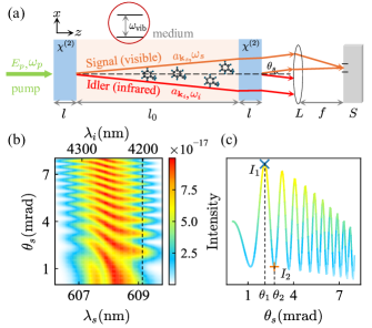
Entanglement-assisted infrared spectroscopic measurement.—We consider the setup of entanglement-assisted infrared spectroscopic measurement [25], as depicted in Fig. 1(a). In this setup, a strong pump field with amplitude and angular frequency from a continuous-wave laser is applied to a nonlinear crystal of length to induce the SPDC process, in which the quadratic susceptibility describes the strength of the interaction between the pump field and the crystal. This crystal is configured to generate entangled photon pairs with signal photons in the visible optical range at frequency , and idler photons in the infrared optical range at frequency . Under a weak SPDC process, the quantum state of these signal-idler photons is [43]
| (1) |
where is the creation operator of signal (idler) light with wave vector , and is the probability amplitude for creating a pair of signal and idler photons with specific wave vectors and . The entangled signal-idler photons then propagate towards a chamber of length , in which the medium (e.g., gas with infrared vibration frequency ) is transparent to visible light and absorbs light in the infrared region, namely [44],
| (2) |
and
| (3) |
with as the annihilation operator of the vacuum environment. Here, are the phases introduced by the propagation of the signal and idler lights in the crystal and medium. are the wave vectors in the medium, with magnitudes , where and are the refractive indices of the crystal and medium, respectively. and are the distance vectors in the crystal and the medium. And is the amplitude transmissivity of the medium for the idler photons, with as its amplitude absorption coefficient.
After propagating through the medium, the pump field interacts with an identical crystal and induces a second SPDC process, generating additional entangled photon pairs. These entangled photons from the two crystals are imaged by a lens () onto the input slit of a visible-light spectrometer (), which is positioned at the lens’s focal length (). The slit of the spectrometer allows signal photons with an emission angle to enter and separates them based on different wavelengths , forming a two-dimensional wavelength-angle intensity distribution. This two-dimensional intensity distribution is determined by the average number of photons of the output signal light [45, 43], i.e.,
| (4) | |||||
where
| (5) | |||||
is the output state of system, with as the vacuum state for the signal, idler and environment modes. The phase term, , is introduced by the propagation of the pump field, in which and are the wave vectors of the pump field within the crystal and the medium, respectively. Here, and are the phase mismatches that arise due to the wave vector mismatches and in the crystal and the medium, with and as the wave vectors of the signal-idler photons along the direction, respectively. The dependence of intensity on emission angle and wavelength is reflected in the expression for the phase mismatches and , whose explicit forms are given in the Supplementary Materials [43]. These two phase mismatches ultimately lead to the occurrence of the interference pattern observed in the visible-light spectrometer.
| Parameters | Values |
|---|---|
| Wavelength of the pump light | 532 nm |
| Quadratic susceptibility | 20 pm/V |
| Crystal length | 0.5 mm |
| Chamber length | 25 mm |
| Amplitude absorption coefficient | 0.15 |
| Refractive indexes | 1/1/ |
| Refractive indexes | 2.3232/2.2930/2.1052 |
The output intensity of the signal light is illustrated as functions of its wavelength and emission angle in Fig. 1(b), with system parameters provided in Table 1. It is clear that the output intensity exhibits distinct bright and dark stripes within the visible wavelength range of the signal light, as shown by the dashed line in Fig. 1(b) and its corresponding cross-section in Fig. 1(c). By measuring the output intensities of the signal light with different emission angles and then fitting these measurement data using Eq. (4), the refractive index and absorption coefficient of the medium for the infrared-idler photons are inferred simultaneously in the experiment [25].
Precision of joint measurement of refractive index and absorption coefficient.—The output intensity of the visible-signal light is correlated with the refraction and absorption properties of the medium for the infrared-idler light, enabling the joint measurement of these two parameters. By selecting two intensities, and , corresponding to different emission angles [e.g., at the peak and at the valley, as illustrated in Fig. 1 (c)] in the output intensity spectrum of the signal light as observables, the joint measurement precisions of the refraction index and absorption coefficient are determined by the following covariance matrix [46, 47, 43],
| (6) |
in which and are their measurement variances, and is covariance, respectively. Here, is the variance of the output signal photons with specific wave vector , and is the number of repeated measurements in the experiment. Additionally, the precision of the joint measurement is bounded by the quantum Cramér-Rao inequality in parameter estimation theory [48, 49, 50, 51, 52, 53], that is,
| (7) |
in which the matrix with elements
| (8) | |||||
is the quantum Fisher information matrix, representing the maximum information about the refractive index and absorption coefficient that can be extracted from all measurement methods. denotes the real part, and are abbreviations for and , with , respectively.
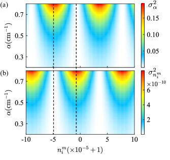
Figures 2 (a) and (b) illustrate the dependence of the measurement variances and on refractive index and absorption coefficient , respectively. We demonstrate that when is fixed, the two variances exhibit oscillatory behavior as varies; whereas, for a constant , they attain a smaller value in the range of weak absorption . It is important to mention that the positions of the refractive index for the two minimum variances and are different. Specifically, the refractive index that minimizes approximately corresponds to the refractive index that maximizes , and vice versa, as shown by the dashed lines in Figs. 2 (a) and (b). This implies that when jointly measuring the refractive index and absorption coefficient, there is a trade-off relation between their measurement precisions, which prevents them from reaching their minimum values simultaneously.
Trade-off relation.—To reveal the trade-off relation between the measurement precisions of refractive index and absorption coefficient, we here define the regret [41] of Fisher information based on Eq. (7), namely,
| (9) |
in which the repeat measurement number is set to without loss of generality. This Fisher information regret characterizes the gap between the quantum Fisher information and the information extracted from the joint measurement regarding these two parameters to be estimated. By introducing the normalized regret of Fisher information, i.e., , we demonstrate that for the case of close emission angles (), the normalized regrets of Fisher information for the refractive index and absorption coefficient in their joint measurement are derived as [43]
| (10) |
and
| (11) |
respectively. Here and are the phase mismatches corresponding to . We find that the two normalized regrets of Fisher information satisfy the following trade-off relation,
| (12) |
Meanwhile, considering the two intensities and that correspond to the peak and valley in the output intensity spectrum of the signal light, Eq. (4) indicates that the term and the term . This leads to a simplified trade-off relation, namely, . Additionally, when the two intensities correspond to different peaks, the trade-off relation becomes as . And when the two intensities correspond to different valleys, the relation is . This clearly demonstrates that for strong absorption media with transmissivity , regardless of whether the peak or valley in the output signal intensity is chosen as the observable, the lower bound of the trade-off is approximately . And for weak absorption media with transmissivity , selecting the output intensities corresponding to different valleys as observables can potentially yield higher joint measurement precisions and a lower bound of the trade-off with relation . However, it is impossible to simultaneously maximize the estimation precisions of these two parameters (i.e., achieving ) under physically permissible scenarios.
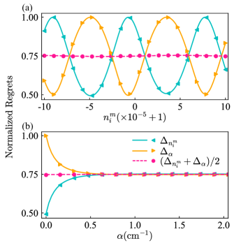
The trade-off relation in Eq. (12) indicates that when jointly measuring the refractive index and absorption coefficient of a medium for idler light, if more information about the refractive index is extracted by measuring the output intensity of the signal light, then correspondingly, less information about the absorption coefficient will be extracted, and vice versa. To illustrate this relation, the normalized Fisher information regrets and are plotted as functions of and with the intensities at peak and valley as observables, respectively, as shown in Figs. 3(a) and (b). The solid and dashed curves depict the exact values of these normalized Fisher information regrets based on their definitions, whereas the corresponding triangle and dot symbols are their approximate values obtained from Eqs. (10)-(12). From the curves, we can see that as and vary, the two normalized Fisher information regrets exhibit a mutually constraining behavior, while their sum remains approximately around , illustrated with the two dashed lines in figures. It is clear that under this trade-off relation, the estimation precision of one parameter is constrained by the measurement inaccuracy of the other, showing that the estimation precisions of the refractive index and absorption coefficient cannot be maximized simultaneously.
Conclusion.—By introducing multi-parameter estimation theory into spectroscopic measurements, our study reveals the inherent uncertainty in multi-parameter measurements within infrared spectroscopy. This uncertainty imposes precision limits on the joint measurement of multiple parameters, not only in the field of linear spectroscopic measurement, but also potentially in high-order spectroscopic measurements [55]. We have demonstrated that when using entangled photon pairs to jointly measure the refractive index and absorption coefficient in the infrared optical range, a trade-off relation exists between the precisions of these two estimated parameters. Such trade-off relation holds significant implications for the future design of high-precision spectroscopic techniques and quantum sensors, guiding advancements in these fields by highlighting the fundamental limits of spectroscopic multi-parameter measurements.
Acknowledgements.
We thank Dr. Lei Shao for helpful discussions. This work is supported by the Innovation Program for Quantum Science and Technology (Grant No. 2023ZD0300700), the National Natural Science Foundation of China (Grant Nos. U2230203, U2330401, 12088101, 12347123, 12405012), and the Hangzhou Joint Fund of the Zhejiang Provincial Natural Science Foundation of China under Grant No. LHZSD24A050001.References
- Horodecki et al. [2009] R. Horodecki, P. Horodecki, M. Horodecki, and K. Horodecki, Rev. Mod. Phys. 81, 865 (2009).
- Jozsa and Linden [2003] R. Jozsa and N. Linden, Proc. R. Soc. London. Ser. A: Math., Phys. Eng. Sci. 459, 2011 (2003).
- Penrose [1998] R. Penrose, Philos. Trans. R. Soc. London. Ser. A: Math., Phys. Eng. Sci. 356, 1927 (1998).
- Brassard et al. [1998] G. Brassard, I. Chuang, S. Lloyd, and C. Monroe, Proc. Natl. Acad. Sci. 95, 11032 (1998).
- Deutsch [1985] D. Deutsch, Proc. R. Soc. A. 400, 97 (1985).
- Bennett and Brassard [2014] C. H. Bennett and G. Brassard, Theor. Comput. Sci. 560, 175 (2014).
- Gisin and Wolf [1999] N. Gisin and S. Wolf, Phys. Rev. Lett. 83, 4200 (1999).
- Dür et al. [1999] W. Dür, H.-J. Briegel, J. I. Cirac, and P. Zoller, Phys. Rev. A 59, 169 (1999).
- Giovannetti et al. [2006] V. Giovannetti, S. Lloyd, and L. Maccone, Phys. Rev. Lett. 96, 010401 (2006).
- Giovannetti et al. [2011] V. Giovannetti, S. Lloyd, and L. Maccone, Nat. Photonics 5, 222 (2011).
- Pezze et al. [2018] L. Pezze, A. Smerzi, M. K. Oberthaler, R. Schmied, and P. Treutlein, Rev. Mod. Phys. 90, 035005 (2018).
- Demkowicz-Dobrzański and Maccone [2014] R. Demkowicz-Dobrzański and L. Maccone, Phys. Rev. Lett. 113, 250801 (2014).
- Riedel et al. [2010] M. F. Riedel, P. Böhi, Y. Li, T. W. Hänsch, A. Sinatra, and P. Treutlein, Nature 464, 1170 (2010).
- Cleve and Buhrman [1997] R. Cleve and H. Buhrman, Phys. Rev. A 56, 1201 (1997).
- Buhrman et al. [2001] H. Buhrman, R. Cleve, and W. Van Dam, SIAM J. Comput. 30, 1829 (2001).
- Brukner et al. [2004] Č. Brukner, M. Żukowski, J.-W. Pan, and A. Zeilinger, Phys. Rev. Lett. 92, 127901 (2004).
- Ursin et al. [2007] R. Ursin, F. Tiefenbacher, T. Schmitt-Manderbach, H. Weier, T. Scheidl, M. Lindenthal, B. Blauensteiner, T. Jennewein, J. Perdigues, P. Trojek, et al., Nat. Phys. 3, 481 (2007).
- Gisin and Thew [2007] N. Gisin and R. Thew, Nat. Photonics 1, 165 (2007).
- Yuan et al. [2010] Z.-S. Yuan, X.-H. Bao, C.-Y. Lu, J. Zhang, C.-Z. Peng, and J.-W. Pan, Phys. Rep. 497, 1 (2010).
- Casacio et al. [2021] C. A. Casacio, L. S. Madsen, A. Terrasson, M. Waleed, K. Barnscheidt, B. Hage, M. A. Taylor, and W. P. Bowen, Nature 594, 201 (2021).
- Belsley [2023] A. Belsley, Phys. Rev. Lett. 130, 133602 (2023).
- Shi et al. [2020] H. Shi, Z. Zhang, S. Pirandola, and Q. Zhuang, Phys. Rev. Lett. 125, 180502 (2020).
- Li et al. [2023] Q. Li, K. Orcutt, R. L. Cook, J. Sabines-Chesterking, A. L. Tong, G. S. Schlau-Cohen, X. Zhang, G. R. Fleming, and K. B. Whaley, Nature 619, 300 (2023).
- Brida et al. [2010] G. Brida, M. Genovese, and I. Ruo Berchera, Nat. Photonics 4, 227 (2010).
- Kalashnikov et al. [2016] D. A. Kalashnikov, A. V. Paterova, S. P. Kulik, and L. A. Krivitsky, Nat. Photonics 10, 98 (2016).
- Okamoto et al. [2020] R. Okamoto, Y. Tokami, and S. Takeuchi, New J. Phys. 22, 103016 (2020).
- Zhang et al. [2024] Z. Zhang, X. Zhang, J. Liu, and H. Dong, arXiv: 2408.13817 [quant-ph] (2024).
- Schawlow [1982] A. L. Schawlow, Rev. Mod. Phys. 54, 697 (1982).
- Jackson and Mantsch [1995] M. Jackson and H. H. Mantsch, Crit. Rev. Biochem. Mol. Biol. 30, 95 (1995).
- Gremlich and Yan [2000] H.-U. Gremlich and B. Yan, Infrared and Raman spectroscopy of biological materials (CRC press, 2000).
- Barbara [2004] S. H. Barbara, Infrared spectroscopy: fundamentals and applications (John Wiley & Sons, 2004).
- Solarz and Paisner [2017] R. W. Solarz and J. A. Paisner, Laser spectroscopy and its applications (Routledge, 2017).
- Paterova et al. [2018] A. Paterova, H. Yang, C. An, D. Kalashnikov, and L. Krivitsky, New J. Phys. 20, 043015 (2018).
- Paterova et al. [2017] A. Paterova, S. Lung, D. A. Kalashnikov, and L. A. Krivitsky, Sci. Rep. 7, 42608 (2017).
- Rogalski [2000] A. Rogalski, Infrared detectors (CRC press, 2000).
- Rogalski [2003] A. Rogalski, Prog. Quant. Electron. 27, 59 (2003).
- Karim and Andersson [2013] A. Karim and J. Y. Andersson, IOP Conf. Ser.: Mater. Sci. Eng. 51, 012001 (2013).
- Keyes [2013] R. J. Keyes, Optical and infrared detectors, Vol. 19 (Springer Science & Business Media, 2013).
- Heisenberg [1983] W. Heisenberg, The physical content of quantum kinematics and mechanics (Princeton University Press Princeton, 1983) pp. 62–84.
- Busch et al. [2007] P. Busch, T. Heinonen, and P. Lahti, Phys. Rep. 452, 155 (2007).
- Lu and Wang [2021] X.-M. Lu and X. Wang, Phys. Rev. Lett. 126, 120503 (2021).
- Xia et al. [2023] B. Xia, J. Huang, H. Li, H. Wang, and G. Zeng, Nat. Commun. 14, 1021 (2023).
- [43] See supplemental material for additional details of derivation and calculation.
- Weedbrook et al. [2012] C. Weedbrook, S. Pirandola, R. García-Patrón, N. J. Cerf, T. C. Ralph, J. H. Shapiro, and S. Lloyd, Rev. Mod. Phys. 84, 621 (2012).
- Klyshko [1993] D. Klyshko, JETP 104, 2676 (1993).
- Paris [2009] M. G. Paris, Int. J.Quantum Inform. 7, 125 (2009).
- Barlow [1993] R. J. Barlow, Statistics: a guide to the use of statistical methods in the physical sciences, Vol. 29 (John Wiley & Sons, 1993).
- Cramér [1999] H. Cramér, Mathematical methods of statistics (Princeton university press, 1999).
- Fisher [1923] R. A. Fisher, Proc. R. Soc. Edinburgh 42, 321 (1923).
- Helstrom [1976] C. W. Helstrom, Quantum detection and estimation theory (Academic Press, 1976).
- Holevo [1982] A. S. Holevo, Probabilistic and statistical aspects of quantum theory (North-Holland Publishing Company, 1982).
- Braunstein and Caves [1994] S. L. Braunstein and C. M. Caves, Phys. Rev. Lett. 72, 3439 (1994).
- Liu et al. [2020] J. Liu, H. Yuan, X.-M. Lu, and X. Wang, J. Phys. A: Math. Theor. 53, 023001 (2020).
- Zhao et al. [2020] J. Zhao, C. Ma, M. Rüsing, and S. Mookherjea, Phys. Rev. Lett. 124, 163603 (2020).
- Mukamel [1995] S. Mukamel, Principles of Nonlinear Optical Spectroscopy (Oxford University Presss, New York, 1995).