Singularity resolution and regular black hole formation in gravitational collapse in asymptotically safe gravity

Abstract

We adopt an effective action inspired by asymptotically safe gravity, in which the effective gravitational constant is parameterized as $G(\epsilon)=G_{N}[1+\tilde{\omega}(G_{N}^{2}\epsilon)^{\alpha}]^{-1}$, where $G_{N}$ and $\epsilon$ denote Newton’s gravitational constant and the energy density of the matter field, respectively, with two dimensionless model parameters, $\tilde{\omega}$ and $\alpha$. Within this framework, we investigate the complete gravitational collapse of a homogeneous ball of perfect fluid and find that the singularity is completely resolved for $\alpha>1$ but not for $1/2\leq\alpha\leq 1$. The case $0<\alpha<1/2$ is inconsistent with asymptotic safety. Moreover, we note that although the singularity cannot be fully resolved for $\alpha=1$, it is significantly weakened by quantum gravity effects. Furthermore, we successfully construct a static exterior metric which, together with the interior solution, describes the dynamical formation of regular black holes in an asymptotically flat spacetime for the perfectly resolved case $\alpha>1$. The resulting regular black hole, obtained as the final static state, contains a de Sitter core and admits a static metric fully expressible in terms of the Lerch transcendent for general cases and in elementary functions for certain values of $\alpha$, including $\alpha=2$. We also discuss the formation of gravastars and the late-time evaporation process of the regular black holes.

I Introduction

Although general relativity (GR) is the simplest and most successful theory of gravity at large distance scales, the presence of spacetime singularities signals the breakdown of its classical description at short distance scales. This suggests the necessity of a quantum theory of gravity. However, a fundamental challenge in constructing such a theory is that GR is well known to be perturbatively nonrenormalizable, which limits its predictive power in a quantum framework.

Recently, asymptotically safe gravity Reuter (1998); Souma (1999); Percacci (2017); Reuter and Saueressig (2018) has emerged as a promising and consistent approach to quantum gravity within the framework of quantum field theory, first proposed by Weinberg Weinberg (1980). This theory is based on the existence of a non-trivial fixed point of the dimensionless coupling constants in the ultraviolet (UV) regime, ensuring that the theory remains UV-complete and predictive, following the Wilsonian approach to renormalization flow. Furthermore, nonperturbative renormalization group (RG) flow equations predict that the RG trajectories of the dimensionless gravitational constant and the cosmological constant flow towards this fixed point, rendering the Einstein-Hilbert action nonperturbatively renormalizable, unlike in traditional perturbative approaches.

In the context of asymptotic safety, the existence of a non-trivial fixed point implies that Newton’s gravitational constant vanishes at high energies, leading to a weakening of gravity at such scales. This has profound implications for various phenomena in black hole physics and the resolution of singularities.

In classical GR, singularity theorems have demonstrated that spacetime singularities are inevitable in various strong gravity scenarios, including complete gravitational collapse under physically reasonable assumptions Penrose (1965); Hawking and Penrose (1970); Hawking and Ellis (2023); Wald (1984). Conventional physics breaks down at spacetime singularities, and in quantum gravity, singularities are expected to be either resolved or at least properly addressed. If singularities are to be resolved in quantum gravity, then the final product of gravitational collapse cannot be a singular black hole but must be something else. Black holes with horizons but without singularities are referred to as regular black holes.

The first notable examples of such objects were provided in Ref. Bardeen (1968); Hayward (2006). For an assessment of the physical properties of several interesting regular black holes, see Ref. Maeda (2022) and references therein. Inspired by asymptotically safe gravity, the resolution of spacetime singularities has been explored in Refs. Bonanno et al. (2017); Chen et al. (2022, 2024, 2023), where the gravitational constant in the metric is replaced by an effective one. However, this substitution is somewhat ad hoc.

Regular black holes typically exhibit a de Sitter core. On the other hand, highly compact objects with a de Sitter core but without horizons can also be constructed; these are known as gravastars Mazur and Mottola (2004); Visser and Wiltshire (2004). While early models of gravastars involved singular hypersurfaces, these are not essential ingredients. Recently, a field-theoretical construction of gravastars has been achieved, ensuring continuity in all physical quantities Ogawa and Ishihara (2023, 2024).

Rather than arbitrarily modifying the gravitational constant in the metric, an alternative approach is to modify the coupling constants in the effective action by introducing a scale-dependent formulation and studying the effects of quantum gravity on the solutions of this effective action. One pioneering study follows the so-called Brans-Dicke approach Reuter and Weyer (2004).

In a different framework developed by Markov and Mukhanov Markov and Mukhanov (1984), matter-gravity coupling is introduced as a scalar function of the fluid’s energy density, $\epsilon$, within the action. This approach naturally determines the effective gravitational and cosmological constants, $G=G(\epsilon)$ and $\Lambda=\Lambda(\epsilon)$, as functions of the energy density. Bonanno et al. Bonanno et al. (2024) applied this approach within the context of asymptotically safe gravity, specifying the precise form of $G$ based on the running of the gravitational constant with a physically motivated cut-off scale. Their analysis demonstrated that this mechanism resolves the spacetime singularity in the marginally bound collapse of a homogeneous dust ball. A similar approach has also been applied to cosmology Zholdasbek et al. (2024).

However, no consistent formation of regular black holes with a de Sitter core has been demonstrated in the context of asymptotically safe gravity, whereas such solutions have been proposed in other gravitational theories in higher dimensions Bueno et al. (2024a, b).

In this paper, we investigate the gravitational collapse of a uniform ball of perfect fluid within the effective action framework of Ref. Bonanno et al. (2024), introducing an index parameter, $\alpha$, that parameterizes the effective gravitational constant. The choice of $\alpha=1$ corresponds to the model used in Ref. Bonanno et al. (2024).

We find that singularity resolution is complete for $\alpha>1$, whereas for $0<\alpha\leq 1$, resolution is impossible in the gravitationally unbound case. For $\alpha>1$, the final static regular structures are regular black holes and gravastars in unbound and marginally bound cases, whereas a static uniform core forms in the bound case. These results indicate that singularity resolution depends strongly on the choice of the cut-off scale in the running gravitational constant within the framework of asymptotically safe gravity.

This paper is organized as follows. In Sec. II, we present the Markov-Mukhanov formulation of the quantum gravity-corrected action and derive the dynamical equations for the Friedmann-Lemaître-Robertson-Walker (FLRW) spacetime. In Sec. III, we discuss the behavior of the effective gravitational and cosmological constants and the resolution of singularities in the FLRW spacetime for different values of the index parameter $\alpha$. In Sec. IV, we examine the metric in the exterior region and the formation of regular black holes and gravastars. In Sec. V, we explore the evaporation of regular black holes and the interpretation of the exterior metric. Finally, Sec. VI presents our conclusions. In Appendix A, we prove (non-)conservation of the bare matter field. In Appendix B, we discuss a physically interesting model that can be treated analytically. In Appendix C, we derive the junction conditions.

Throughout this paper, we use the sign convention of Wald Wald (1984) and units where $c=\hbar=k=1$. Newton’s gravitational constant or the Planck mass, $G_{N}=m_{P}^{-2}$, is retained explicitly throughout the discussion.

II Formulation

II.1 Markov-Mukhanov formulation of the effective action

The action for an isentropic perfect fluid in Einstein gravity can be written in Ref. Hawking and Ellis (2023) as

$$S=\frac{1}{16\pi G_{N}}\int d^{4}x\sqrt{-g}[R-16\pi G_{N}\epsilon],$$ (1)

In this action, $\epsilon$ is a function of $n$, i.e., $\epsilon=\epsilon(n)$, where $n$ is the conserved number density. The number conservation $\nabla_{\mu}(nu^{\mu})=0$ is required with $u^{\mu}$ being the four-velocity of the fluid. The function $\epsilon(n)$ specifies the equation of state (EOS) through the first law

$$p=n\frac{d\epsilon}{dn}-\epsilon,$$ (2)

which is derived by the variational principle. For example, the EOS $p=w\epsilon$ is realized by the choice $\epsilon=Cn^{1+w}$, where $C$ is a nonzero constant. The variation of the action with respect to the metric gives the Einstein equation

$$G_{\mu\nu}=8\pi G_{N}T_{\mu\nu},$$ (3)

where the stress-energy tensor is derived as

$$T_{\mu\nu}=(\epsilon+p)u_{\mu}u_{\nu}+pg_{\mu\nu},$$ (4)

which satisfies the conservation law

$$\nabla_{\mu}T^{\mu\nu}=0.$$ (5)

To discuss the effect of quantum gravity to the cosmological expansion in the early Universe, Markov and Mukhanov Markov and Mukhanov (1984) introduced an effective action

$$S=\frac{1}{16\pi G_{N}}\int d^{4}x\sqrt{-g}[R-2\chi(\epsilon)\epsilon],$$ (6)

where $\epsilon$ is the “bare” energy density of the perfect fluid. The function $\chi(\epsilon)$ denotes the quantum correction. If $\chi(\epsilon)=8\pi G_{N}$, then we recover the original action (1). On the other hand, if we put $\chi(\epsilon)\epsilon=8\pi G_{N}\epsilon_{\rm eff}$, then everything goes in the same way as the original system except for $\epsilon$ and $p$ being replaced by $\epsilon_{\rm eff}$ and $p_{\rm eff}$. The first law reduces to

$$p_{\rm eff}=n\frac{d\epsilon_{\rm eff}}{dn}-\epsilon_{\rm eff}.$$ (7)

This gives the relation between $p_{\rm eff}$ and $\epsilon_{\rm eff}$ parameterized by $n$, i.e., the EOS for the effective fluid. So, given a function $\epsilon(n)$, introducing $\chi(\epsilon)$ is nothing but modifying the EOS from the original one $p=p(\epsilon)$ to the effective one $p_{\rm eff}=p_{\rm eff}(\epsilon_{\rm eff})$ from a classical point of view.

The variation with respect to the metric yields

$$G_{\mu\nu}=8\pi G_{N}T_{{\rm eff}\mu\nu},$$ (8)

where the effective stress-energy tensor is given by

$$T_{{\rm eff}\mu\nu}=(\epsilon_{\rm eff}+p_{\rm eff})u_{\mu}u_{\nu}+p_{\rm eff}g_{\mu\nu}$$ (9)

with the effective matter quantities being

$$8\pi G_{N}\epsilon_{\rm eff} = \chi\epsilon,$$ (10)

$$8\pi G_{N}p_{\rm eff} = p\frac{d(\chi\epsilon)}{d\epsilon}+\frac{d\chi}{d\epsilon}\epsilon^{2},$$ (11)

where $p$ is given by Eq. (2). The effective gravitational constant $G(\epsilon)$ and cosmological constant $\Lambda(\epsilon)$ are defined as

$$8\pi G_{N}T_{{\rm eff}\mu\nu}=8\pi G(\epsilon)[(\epsilon+p)u_{\mu}u_{\nu}+pg_{\mu\nu}]-\Lambda(\epsilon)g_{\mu\nu},$$ (12)

so that we can find

$$8\pi G(\epsilon)(\epsilon+p)=8\pi G_{N}(\epsilon_{\rm eff}+p_{\rm eff})$$ (13)

and

$$8\pi G(\epsilon)=\frac{d(\chi(\epsilon)\epsilon)}{d\epsilon},\qquad\Lambda(\epsilon)=-\frac{d\chi(\epsilon)}{d\epsilon}\epsilon^{2}=8\pi G_{N}\epsilon_{\rm eff}-8\pi G(\epsilon)\epsilon.$$ (14)

Inversely, we can uniquely reconstruct $\epsilon_{\rm eff}$ and $p_{\rm eff}$ as

$$8\pi G_{N}\epsilon_{\rm eff}=8\pi\int^{\epsilon}_{0}G(s)ds,\qquad 8\pi G_{N}p_{\rm eff}=8\pi G(\epsilon)(\epsilon+p)-8\pi G_{N}\epsilon_{\rm eff}.$$ (15)

where the integration constant is chosen so that $\epsilon_{\rm eff}=\epsilon$ is recovered for $G(\epsilon)=G_{N}$. We call $\epsilon$ and $p$ the bare energy density and pressure, respectively. The invariance of the action against infinitesimally small coordinate transformation yields the matter conservation law for the effective matter field

$$\nabla_{\mu}T_{\rm eff}^{\mu\nu}=0.$$ (16)

On the other hand, the bare matter field stress-energy tensor neither is required to satisfy the conservation law nor satisfies in general. However, surprisingly, in the FLRW spacetime, the bare conservation law happens to be satisfied due to the high symmetry of the spacetime. We will prove this in Appendix A.

II.2 Effective gravitational constant inspired by asymptotically safe gravity

In the framework of asymptotically safe gravity Reuter (1998), the central element is the gravitational effective average action (EAA), a coarse-grained functional of the metric and a momentum scale $k$, which acts as an infrared cut off. The construction of the EAA involves integrating out all quantum fluctuations with momenta $q^{2}>k^{2}$, while suppressing contributions from modes with $q^{2}<k^{2}$. The evolution of the effective average action is governed by the exact functional renormalization equation, which can be solved by truncating the infinite-dimensional action space into the Einstein-Hilbert truncation. Then, the effective gravitational constant and cosmological constant become scale-dependent, denoted as $G(k)$ and $\Lambda(k)$, respectively. In the ultraviolet (UV) limit, the RG flow approaches a fixed point, where the dimensionless coupling constants attain finite limit values $g(k):=k^{2}G(k)\to g_{*}$ and $\lambda(k):=k^{-2}\Lambda(k)\to\lambda_{*}$ as $k\to\infty$. For a small value of the dimensionless cosmological constant, the RG equations lead to the solution for the Newton coupling, $G(k)={G_{N}}/{(1+\omega G_{N}k^{2})}$, where $\omega$ is a certain positive value of the order of unity Bonanno and Reuter (2000).

To include the above analysis in the spacetime dynamics, the cut-off scale $k$ can be regarded as a function of some physical quantities such as the spacetime curvature scale and some physical length scales. In the FLRW spacetime, the curvature scale is completely characterized by the energy density if we fix the EOS. So, it is natural to assume that the cut-off scale is a function of the bare energy density $\epsilon$, i.e., $k=k(\epsilon)$, and identify the scale-dependent coupling constants $G(k(\epsilon))$ and $\Lambda(k(\epsilon))$ with $G(\epsilon)$ and $\Lambda(\epsilon)$ in the Markov-Mukhanov formulation. However, there is no prior relationship between $G(k),\Lambda(k)$ and $G(\epsilon),\Lambda(\epsilon)$. In this paper, we parameterize the effective gravitational constant by two positive dimensionless parameters $\tilde{\omega}$ and $\alpha>0$ such that

$$G(\epsilon)=\frac{G_{N}}{1+\omega G_{N}k^{2}}=\frac{G_{N}}{1+\tilde{\omega}(G_{N}^{2}\epsilon)^{\alpha}}.$$ (17)

In other words, we infer the following identification of the cut-off scale $k$ as

$$\omega G_{N}k^{2}=\tilde{\omega}(G_{N}^{2}\epsilon)^{\alpha}.$$ (18)

A larger $\tilde{\omega}$ implies a lower quantum gravity scale in terms of $\epsilon$ at which quantum gravity effects begin to affect the system, while a larger $\alpha$ gives stronger quantum-gravity effects for $\epsilon\to\infty$. The dimensionless constant $\tilde{\omega}$ is not necessarily of the order of unity.

It is not so straightforward to determine the index $\alpha$. We should note that $\alpha=1$ is chosen for the FLRW spacetime in Ref. Bonanno et al. (2024) by an argument on the proper distance to the center of the Schwarzschild black hole in Ref. Bonanno and Reuter (2000). If we use the scalar curvature polynomials such as the Kretschmann invariant ${\cal K}=R^{\mu\nu\rho\sigma}R_{\mu\nu\rho\sigma}$ for scale identification, we find $k\sim{\cal K}^{1/4}\sim(G_{N}\epsilon)^{1/2}$ in classical dynamics, so that we reach $\alpha=1$. On the other hand, a simplistic dimensional argument might imply $\alpha=1/2$ because $\epsilon$ has mass dimension of $4$, in which the relation (18) need not involve $G_{N}$. This seems to be consistent with the choice in Ref. Bonanno et al. (2017). It is also interesting that the coarse gaining scale $k=\sigma H$ is naturally introduced in the framework of stochastic inflation in terms of the physical proper wave number $k$ with $\sigma\sim 0.1$, where $H$ is the Hubble parameter Starobinsky (1982, 1986). If we identify this coarse gaining scale with that in asymptotically safe gravity, $\alpha=1$ will again be preferred because $k=\sigma H\sim\sigma(G_{N}\epsilon)^{1/2}$ using the Einstein equation. Furthermore, we may have to consider that the modified physical spacetime is governed by not the bare values $\epsilon$ and $p$ but the effective ones $\epsilon_{\rm eff}$ and $p_{\rm eff}$. In fact, later in this paper, we will discuss that $\alpha>1$ is favored from a singularity resolution point of view. Incidentally, although we cannot expect that the simple functional form given in Eq. (17) should hold across all the energy scales $0<\epsilon<\infty$, physical results about singularity resolution discussed in this paper will not depend on the detailed functional form but on the asymptotic behaviors in the limit of $\epsilon\to\infty$.

In the framework of Markov and Mukhanov for a given energy density $\epsilon=\epsilon(n)$, if we fix the effective gravitational constant $G(\epsilon)$, we will obtain the effective cosmological constant $\Lambda(\epsilon)$ by Eq. (14). The dimensionless cosmological constant

$$\lambda(k)=\frac{\Lambda(k)}{k^{2}}=\frac{\omega G_{N}\Lambda(\epsilon)}{\tilde{\omega}(G_{N}^{2}\epsilon)^{\alpha}}$$ (19)

must have a finite value limit for the consistency with the RG flow giving asymptotic safety. So, this can be regarded as an additional condition for the physical effective gravitational constant $G(\epsilon)$.

II.3 Collapsing FLRW interior

Bonanno et al. Bonanno et al. (2024) assume spherical symmetry for the whole spacetime and homogeneity in the interior and staticity in the exterior. Spherical symmetry and homogeneity directly imply the FLRW spacetime irrespective of gravitational theories. So, we assume the FLRW metric

$$ds^{2}=-d\tau^{2}+a^{2}(\tau)\left(\frac{dr^{2}}{1-Kr^{2}}+r^{2}d\Omega^{2}\right),$$ (20)

where $d\Omega^{2}$ is the metric on the unit two-sphere and $K$ is constant corresponding to the spatial curvature. The collapse solutions with $K>0$, $K=0$ and $K<0$ are said to be gravitationally bound, marginally bound and unbound, respectively, and all are physically acceptable because $K$ is determined just by the initial conditions. We further assume the EOS $p=w\epsilon$ for the bare perfect fluid with $w$ being a nonnegative constant. In the current collapse model, the Hamiltonian constraint of the modified Einstein equation reduces to

$$\dot{a}^{2}+V(a)+K=0,$$ (21)

where $V(a)$ and $\epsilon_{\rm eff}$ are given by

$$V(a) = -\frac{a^{2}}{3}8\pi G_{N}\epsilon_{\rm eff}(a),$$ (22)

$$8\pi G_{N}\epsilon_{\rm eff} = 8\pi\int^{\epsilon}_{0}G(s)ds=8\pi G_{N}^{-1}\tilde{\omega}^{-1/\alpha}I_{\alpha}(x),$$ (23)

where we have defined

$$I_{\alpha}(x):=\int^{x}_{0}\frac{d\tilde{x}}{1+\tilde{x}^{\alpha}},$$ (24)

with $x=\tilde{\omega}^{1/\alpha}G_{N}^{2}\epsilon$. We should note that $V(a)\leq 0$ since $I_{\alpha}(x)\geq 0$. The integral in Eq. (24) can be implemented as

$$I_{\alpha}(x)=x~_{2}F_{1}\left(1,\frac{1}{\alpha};1+\frac{1}{\alpha};-x^{\alpha}\right)=\frac{x}{\alpha}\Phi\left(-x^{\alpha},1,\frac{1}{\alpha}\right);\quad\Phi(z,s,\alpha)=\sum_{n=0}^{\infty}\frac{z^{n}}{(n+\alpha)^{2}},$$ (25)

where $\Phi$ is called the Lerch transcendent or the LerchPhi. For example, for $\alpha=1/2$, $1$ and $2$, this can be expressed by elementary functions as follows:

$$I_{1/2}(x)=2[\sqrt{x}-\ln(\sqrt{x}+1)],\quad I_{1}(x)=\ln(1+x),\quad I_{2}(x)=\arctan(x).$$ (26)

For any value of $\alpha$, for $0<x\ll 1$, we find $I_{\alpha}(x)\approx x$. For $x\gg 1$, for $0<\alpha<1$, the integral can be estimated as $I_{\alpha}(x)\approx x^{1-\alpha}/(1-\alpha)$, while for $\alpha>1$, the integral converges for $x\to\infty$ as

$$\lim_{x\to\infty}I_{\alpha}(x)=\int_{0}^{\infty}\frac{1}{1+\tilde{x}^{\alpha}}d\tilde{x}=:{\mathscr{C}}_{\alpha}.$$ (27)

The evolution equations together with the Hamiltonian constraint of the Einstein equation give

$$\frac{\ddot{a}}{a}=-\frac{4\pi}{3}G_{N}(\epsilon_{\rm eff}+3p_{\rm eff}).$$ (28)

For the FLRW spacetime, obtaining the solution to the conservation of the number current and substituting it into the bare value $\epsilon=\epsilon(n)$ yield

$$n=\frac{n_{1}}{a^{3}},\qquad\epsilon=\frac{\epsilon_{1}}{a^{3(1+w)}},$$ (29)

where $n_{1}$ and $\epsilon_{1}$ are constants of integration. See Appendix A for the conservation law of the bare fluid. The resulting potentials for $\alpha=1/2$, $1$ and $2$ for $w=1/3$ are plotted in Fig. 1. We can see that the modified potential has a negative minimum and approaches $0$ for $\alpha=1$ and $\alpha=2$ or a negative finite value for $\alpha=1/2$ as $a\to 0$, whereas the potential in GR diverges to $-\infty$ in the same limit. Then, it follows from Eq. (21) that $a=0$ can be avoided for $K>0$ but is inevitable for $K<0$ even for the modified case, whereas it is inevitable for all cases in GR. We will see this more carefully in Sec. III.

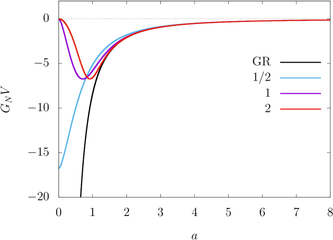
Figure 1: The effective potential $V(a)$ for $\alpha=1/2$, $1$ and $2$ for the EOS parameter $w=1/3$, where $\tilde{\omega}=1$ and $G_{N}^{2}\epsilon_{1}=1$ are fixed. Each curve with quantum modification is labeled with the value of $\alpha$. The potential approaches $0$ in the limit $a\to\infty$ for $\alpha>0$, while in the limit $a\to 0$ it approaches $0$ for $\alpha\geq 1$ but a finite negative value for $\alpha=1/2$. We can see that the potential has the only one minimum for $\alpha=1$ and $2$.

As for the limit of $a\to\infty$, because of the behavior of the integral for $0<x\ll 1$, we find

$$V(a) \approx -\frac{8\pi G_{N}}{3}\frac{\epsilon_{1}}{a^{1+3w}},$$ (30)

$$\epsilon_{\rm eff} \approx \epsilon=\frac{\epsilon_{1}}{a^{3(1+w)}},$$ (31)

irrespective of the value of $\alpha$.

The FLRW spacetime has vanishing Weyl curvature and the remaining Riemann tensor is written by the Ricci tensor. All the scalar curvature polynomials are written solely by $\epsilon_{\rm eff}$ and $p_{\rm eff}$. See, e.g., Ref. Harada et al. (2018, 2022).

III Singularity resolution

Here, we will discuss singularity resolution in the FLRW spacetime in the context of gravitational collapse. We should note, however, that the present analysis also immediately applies to resolution of big-bang singularities just by taking time reversal.

III.1 Effective gravitational and cosmological constants

We plot the effective gravitational and cosmological constants, $G(\epsilon)$ and $\Lambda(\epsilon)$, as functions of $\epsilon$ for $\alpha=1/2$, $1$ and $2$ in Fig. 2. We can see that $G(\epsilon)$ decreases as $\epsilon$ increases for all $\alpha>0$ but faster than $\epsilon^{-1}$ for sufficiently large $\epsilon$ only for $\alpha>1$. The relationship between the effective and bare stress-energy tensors given by Eq. (12) implies that because of the behavior of $G(\epsilon)$ in the limit of $\epsilon\to\infty$, the contribution of the bare stress-energy tensor to the effective one diverges for $0<\alpha<1$, remain finite for $\alpha=1$ but vanishes for $\alpha>1$. Equations (14) and (15) immediately imply that as $\epsilon\to\infty$, we have $\Lambda(\epsilon)$ proportional to $\epsilon^{1-\alpha}\to\infty$ for $0<\alpha<1$ and to $\ln\epsilon\to\infty$ for $\alpha=1$ but approaches a finite positive value, $\Lambda_{{\rm eff}0}$, for $\alpha>1$. More precise analytical expressions for $\Lambda(\epsilon)$ in the limit $\epsilon\to\infty$ will be given in Sec. III.3. Thus, we can conclude that only for $\alpha>1$, the contribution of the bare matter field is being lost, so that the effective fluid mimics the cosmological constant in a high-energy regime. The above discussion will not depend on the details of the EOS of the fluid.

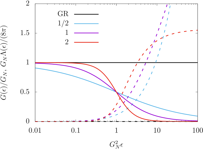
Figure 2: The effective gravitational and cosmological constants, $G(\epsilon)$ and $\Lambda(\epsilon)$, are plotted with the solid line and the dashed line, respectively, as functions of $\epsilon$ for $\alpha=1/2$, $1$ and $2$, where $\tilde{\omega}=1$ is fixed. Each curve with quantum modification is labeled with the value of $\alpha$.

III.2 Effective energy density and pressure

The behavior of $\epsilon_{\rm eff}$ and $p_{\rm eff}$ as functions of $\epsilon$ is plotted for $\alpha=1/2$, $1$ and $2$ and $w=1/3$ in Fig. 3. In this figure, we can see that the asymptotic safety significantly slows down the increase in $\epsilon_{\rm eff}$ as $\epsilon$ is increased. We can also see that $\epsilon_{\rm eff}$ grows up together with $\epsilon$ for $\alpha=1/2$ and $\alpha=1$ but approaches a constant value $\epsilon_{{\rm eff}0}$ for $\alpha=2$, where $\Lambda_{{\rm eff}0}=8\pi G_{N}\epsilon_{{\rm eff}0}$. In fact, Eq. (23) together with the property of the integral $I_{\alpha}(x)$ in the limit of $x\to\infty$ implies that the divergence of $\epsilon$ in finite proper time directly leads to curvature singularity for $0<\alpha\leq 1$ but not for $\alpha>1$. The $\epsilon_{\rm eff}$ and $p_{\rm eff}$ go to $+\infty$ and $-\infty$ as $\epsilon$ increases to $+\infty$ for $0<\alpha\leq 1$ but take finite limit values $\epsilon_{{\rm eff}0}$ and $p_{{\rm eff}0}=-\epsilon_{{\rm eff}0}$ for $\alpha>1$ according to Eq. (15), respectively. This implies that the divergence of $\epsilon_{\rm eff}$ is resolved and the fluid effectively behaves like a cosmological constant in high-energy limit for $\alpha>1$, while the divergence is not resolved for $0<\alpha\leq 1$.

In the FLRW spacetime, Eq. (29) follows from the conservation law. Therefore, if $a=0$ is reached in finite proper time $\tau$, it corresponds to curvature singularity for $0<\alpha\leq 1$.

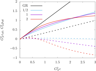
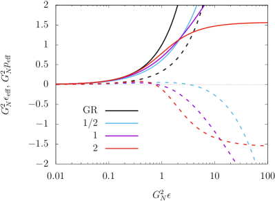
Figure 3: The effective energy density $\epsilon_{\rm eff}$ and $p_{\rm eff}$ are plotted with the solid line and the dashed line, respectively, as functions of $\epsilon$ for $\alpha=1/2$, $1$ and $2$ for the EOS parameter $w=1/3$, where $\tilde{\omega}=1$ is fixed. The left and right panels show the smaller range of $\epsilon$ in linear scale and the overall range in log scale, respectively. Each curve with quantum modification is labeled with the value of $\alpha$. We can see that the increase in $\epsilon_{\rm eff}$ slows down due to the quantum effect. The $\epsilon_{\rm eff}$ and $p_{\rm eff}$ continue increasing to $+\infty$ and decreasing to $-\infty$ for $0<\alpha\leq 1$ but take finite limit values $\epsilon_{{\rm eff}0}$ and $-\epsilon_{{\rm eff}0}$ for $\alpha>1$, respectively, as $\epsilon$ increases to $+\infty$. This implies that the divergence of $\epsilon_{\rm eff}$ is resolved and the fluid effectively behaves like a cosmological constant in high-energy limit for $\alpha>1$, while the divergence is not resolved for $0<\alpha\leq 1$.

III.3 Dynamics of the scale factor and singularity resolution

We discuss the behavior of $a(\tau)$ below for the cases $\alpha>1$, $\alpha=1$ and $0<\alpha<1$ separately.

III.3.1 $\alpha>1$

In this case, in the limit of $a\to 0$, or $\epsilon=\epsilon_{1}/a^{3(1+w)}\to\infty$, we have

$$V(a) \approx -\frac{8\pi G_{N}}{3}a^{2}\tilde{\omega}^{-1/\alpha}G_{N}^{-2}{\mathscr{C}}_{\alpha}\to 0,$$ (32)

$$\epsilon_{\rm eff} \to \epsilon_{{\rm eff}0}:=\tilde{\omega}^{-1/\alpha}G_{N}^{-2}{\mathscr{C}}_{\alpha},$$ (33)

$$\Lambda \to \Lambda_{{\rm eff}0}:=8\pi G_{N}\epsilon_{{\rm eff}0}.$$ (34)

Therefore, we deduce that $V(a)$ has a negative minimum $V_{\rm min}$ at $a=a_{\rm min}$. This minimum corresponds to the Einstein static universe with $p_{\rm eff}=-\epsilon_{\rm eff}/3$ with $K=-V_{\rm min}>0$ as seen in Eq. (28) and see Ref. Harada et al. (2018, 2022). We assume that $V(a)$ has the only one minimum. Since $\epsilon_{\rm eff}$ is a monotonically decreasing function of $a$, $\epsilon_{\rm eff}$ is bounded from above by $\epsilon_{{\rm eff}0}$. We can also derive $p_{\rm eff}\to-\epsilon_{{\rm eff}0}$ as $a\to 0$ so that the effective matter field behaves like a cosmological constant. Thus, we can conclude that any curvature singularity is completely resolved for any values of $K$ and nonnegative values of $w$. In the same limit, we find $\lambda(k)\to 0$. So, this can be consistent with the solution (17) in asymptotically safe gravity.

The dynamics of the scale factor governed by Eq. (21) is summarized as follows. For $K>0$, $a$ cannot reach $0$ because $V(a)+K>0$ in the neighborhood of $a=0$. Generically, $a$ oscillates in the interval including $a_{\rm min}$, whereas there is an exceptional case, where $K+V_{\rm min}=0$. In this latter case, $a$ is constant at $a=a_{\rm min}$ for which we have an Einstein static Universe. Interestingly, this is stable because a small perturbation gives an oscillating solution around $a=a_{\rm min}$. For any cases with $K>0$, the effective fluid does not act as a cosmological constant.

For $K=0$, $a$ can reach $0$. We can see that the collapsing solution behaves like

$$a\approx C\exp\left(-\sqrt{\frac{8\pi G_{N}}{3}\epsilon_{{\rm eff}0}}\tau\right)$$ (35)

as $\tau\to\infty$, where $C$ is a constant of integration. So, it takes infinite proper time for $a=0$ to be reached. In fact, Eq. (35) shows a shrinking de Sitter solution in the flat chart, where the timelike geodesic with a constant $r$ finally reaches null infinity in the limit $\tau\to\infty$ as depicted by the orange line in Fig. 4. This implies the formation of the de Sitter core in the center and this portion is future timelike geodesically complete.

For $K<0$, the potential does not prevent $a$ from reaching $0$ in finite proper time. The solution for $a$ is described by

$$a\approx\sqrt{-K}(\tau_{s}-\tau)$$ (36)

for $a\to 0$, where $\tau=\tau_{s}$ is the time of crossing $a=0$. Although one might regard $\tau=\tau_{s}$ as singularity, it is not. What is really happening is the end point of the open chart in the de Sitter spacetime as depicted by the black filled circle in Fig. 4. In reality, $\tau=\tau_{s}$ is not singularity but a regular point. The spacetime is extended beyond $\tau=\tau_{s}$. In our case, the exterior and the future of the negative curvature FLRW region is given by a regular static metric, which will be discussed later.

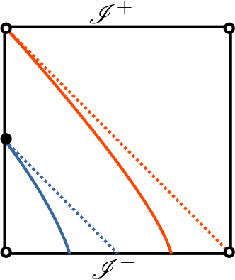
Figure 4: Different charts in the de Sitter spacetime. The global chart ($K>0$) covers the whole de Sitter spacetime, which is depicted by the big black square with the coordinate extension through $r=\sqrt{K}\sin\chi$ and $0\leq\chi<\pi$. The contracting flat chart ($K=0$) covers the left-bottom half below the orange dashed line, while the contracting open chart ($K<0$) covers the left-bottom one-eighth below the blue dashed line. The world lines with fixed comoving coordinate $r$, which are timelike geodesics, in the flat chart and open chart are depicted by the orange solid line and the blue solid line, respectively. All world lines with fixed comoving coordinate in the flat chart reach a point depicted by the open circle in the future infinity in infinite proper time, while those in the open chart terminate at a regular point depicted by the filled circle in finite proper time due to coordinate singularity. See Ref. Sato and Kodama (1992); Griffiths and Podolsky (2009) for details.

III.3.2 $\alpha=1$

For this case, we have

$$V(a)=-\frac{8\pi G_{N}^{-1}}{3}\tilde{\omega}^{-1}a^{2}\ln\left(1+\tilde{\omega}\frac{G_{N}^{2}\epsilon_{1}}{a^{3(1+w)}}\right).$$ (37)

Then, we find

$$\Lambda=8\pi G_{N}^{-1}\tilde{\omega}^{-1}\left[\ln\left(1+\tilde{\omega}G_{N}^{2}\epsilon\right)-\frac{\tilde{\omega}G_{N}^{2}\epsilon}{1+\tilde{\omega}G_{N}^{2}\epsilon}\right].$$ (38)

Thus, $\Lambda(\epsilon)$ shows logarithmic divergence as $\epsilon\to\infty$. The dimensionless cosmological constant is given by

$$\lambda(k)=8\pi\frac{\omega}{\tilde{\omega}}\frac{1}{G_{N}^{2}\epsilon}\left[\ln\left(1+\tilde{\omega}G_{N}^{2}\epsilon\right)-\frac{\tilde{\omega}G_{N}^{2}\epsilon}{1+\tilde{\omega}G_{N}^{2}\epsilon}\right],$$ (39)

which goes to $0$ as $\epsilon\to\infty$, so that the consistency is satisfied. In this case, $V(a)$ approaches $0$ as $a\to 0$, takes the only one minimum $V=V_{\rm min}<0$ at $a=a_{\rm min}$ and approaches $0$ as $a\to\infty$.

The dynamics is summarized as follows. For $K>0$, $a$ cannot reach $0$ because $V(a)+K>0$ in the neighborhood of $a=0$. The solution is an Einstein static Universe or an oscillating solution around it. For $K=0$, it needs infinite proper time for $a=0$ to be reached because the asymptotic solution is given by

$$a\approx C\exp\left[-2\pi(1+w)\tilde{\omega}^{-1}G_{N}^{-1}\tau^{2}\right],$$ (40)

as $\tau\to\infty$, where $C$ is a constant of integration. This can be regarded as singularity resolution, which is noticed by Bonanno et al. Bonanno et al. (2024). For $K<0$, $a$ monotonically decreases and reaches $0$ in finite proper time at $\tau=\tau_{s}$ because $V(a)+K\leq K<0$. Since $V(a)\to 0$ as $a\to 0$, $a$ behaves as $a\approx\sqrt{-K}(\tau_{s}-\tau)$ for $a\to 0$. In this case, $\epsilon_{\rm eff}$ shows divergence, corresponding to curvature singularity. Although singularity occurrence is inevitable for unbound collapse, it deserves great attention that curvature strength of the singularity in this case is significantly weak as the scalar curvature polynomials such as ${\cal K}$ only show logarithmic divergence with respect to the affine parameter in an approach of timelike geodesics to the singularity. See Ref. Clarke (1994) for curvature strength of singularities.

III.3.3 $0<\alpha<1$

In this case, in the limit $a\to 0$, we have $\epsilon\to\infty$,

$$\epsilon_{\rm eff}\approx\frac{1}{1-\alpha}G_{N}^{-2}\tilde{\omega}^{-1}(G_{N}^{2}\epsilon)^{1-\alpha}$$ (41)

and therefore,

$$\Lambda\approx 8\pi G_{N}^{-1}\frac{\alpha}{1-\alpha}\tilde{\omega}^{-1}(G_{N}^{2}\epsilon)^{1-\alpha}.$$ (42)

Thus, $\Lambda(\epsilon)\to\infty$ as $\epsilon\to\infty$. The dimensionless cosmological constant is given by

$$\lambda(k)\approx 8\pi\frac{\omega}{\tilde{\omega}^{2}}\frac{\alpha}{1-\alpha}(G_{N}^{2}\epsilon)^{1-2\alpha}.$$ (43)

Therefore, the consistency requires $\alpha\geq 1/2$ for $\epsilon\to\infty$.

The potential is calculated to give

$$V(a)\approx-\frac{8\pi G_{N}^{-1}}{3}\frac{1}{1-\alpha}\tilde{\omega}^{-1}(G_{N}^{2}\epsilon_{1})^{1-\alpha}a^{2-3(1-\alpha)(1+w)}$$ (44)

as $a\to 0$. We put $\beta:=1-(3/2)(1-\alpha)(1+w)$, where $\beta<1$ holds from the assumption. We separately discuss the dynamics for the cases of $\beta>0$, $\beta=0$ and $\beta<0$ below. The conclusion is that we cannot resolve singularity for $K\leq 0$ in any case.

For $\beta>0$, $V(a)\to 0$ as $a\to 0$ and there exists a negative minimum $V_{\rm min}$ at $a=a_{\rm min}$. Then, for $K>0$, $a=0$ cannot be reached. For $K=0$, we have

$$a\approx\left[(1-\beta)\sqrt{\frac{8\pi G_{N}^{-1}}{3}\frac{\tilde{\omega}^{-1}}{1-\alpha}}\right]^{1/(1-\beta)}(\tau_{s}-\tau)^{1/(1-\beta)}$$ (45)

as $a\to 0$. Thus, the collapse encounters singularity in finite proper time. $K<0$ gives singularity in finite proper time at $\tau=\tau_{s}$, where $a\approx\sqrt{-K}(\tau_{s}-\tau)$ for $a\to 0$.

For $\beta<0$, $V(a)\to-\infty$ as $a\to 0$. In this case, singularity occurs in finite proper time for any value of $K$.

For $\beta=0$, $V(a)\to V_{0}<0$ as $a\to 0$, where

$$V_{0}=-\frac{8\pi G_{N}^{-1}}{3}\frac{1}{1-\alpha}\tilde{\omega}^{-1}(G_{N}^{2}\epsilon_{1})^{1-\alpha}.$$ (46)

For $K+V_{0}>0$, the collapse will not reach $a=0$. For $K+V_{0}<0$, singularity occurs if the collapse starts with sufficiently small $a$. We will relegate the discussion on an intriguing subclass $\alpha=1/2$ and $w=1/3$ to Appendix B.

IV Regular black holes, gravastars and uniform cores

IV.1 Exterior metric

Following the prescription in Ref. Bonanno et al. (2024), we assume a static exterior region with the metric written in the form

$$ds^{2}=-f(R)dt^{2}+\frac{1}{f(R)}dR^{2}+R^{2}d\Omega^{2}$$ (47)

and require smooth matching by imposing the continuity of both the first and second fundamental forms on the boundary hypersurface $r=r_{b}$ between the interior FLRW solution and the exterior. If $f(R)>0$ for $0<R<\infty$, there is no horizon, while $f(R)=0$ at $R=R_{h}$, there is a Killing horizon there. As is shown in Appendix C, it has turned out that the areal radius and the Misner-Sharp mass must be continuous at the matching surface $\Sigma$: $r=r_{b}$ or $R=R_{b}(\tau)=r_{b}a(\tau)$. Following this procedure, putting

$$f(R)=1-\frac{2G_{N}m(R)}{R},$$ (48)

where $m(R)$ is the Misner-Sharp mass, the smooth matching suggests

$$m(R)=\frac{4\pi}{3}R^{3}\epsilon_{\rm eff}\left(\frac{R}{r_{b}}\right)=\frac{4\pi G_{N}^{-2}}{3}R^{3}\tilde{\omega}^{-1/\alpha}I_{\alpha}\left(\frac{\tilde{\omega}^{1/\alpha}G_{N}^{2}\epsilon_{1}r_{b}^{3(1+w)}}{R^{3(1+w)}}\right),$$ (49)

where $\epsilon_{\rm eff}=\epsilon_{\rm eff}(a)$ and the concrete expression for $I_{\alpha}(x)$ is given by Eq. (25). Strictly speaking, the junction condition only determines $m(R)$ for the range that the junction surface sweeps, so the above metric should be regarded as analytic continuation if we use it beyond that range.

Irrespective of the value of $\alpha$, we can derive the asymptotic form of $m(R)$ in the limit $R\to\infty$ as

$$m(R)\approx 4\pi\frac{\epsilon_{1}r_{b}^{3(1+w)}}{3R^{3w}}.$$ (50)

Therefore, if $w\geq 0$, the spacetime is asymptotically flat. For $w=0$, the ADM mass $M$ is given by $M=({4\pi}/{3})\epsilon_{1}r_{b}^{3}$, while $M=0$ for $w>0$. Inspired by the above, we define $M_{w}=({4\pi}/{3})\epsilon_{1}r_{b}^{3(1+w)}$ so that $M_{0}=M$ and $m(R)\approx{M_{w}}/{R^{3w}}$ as $R\to\infty$. Using this, we can rewrite $m(R)$ as

$$m(R)=\frac{4\pi G_{N}^{-2}}{3}R^{3}\tilde{\omega}^{-1/\alpha}I_{\alpha}\left(\tilde{\omega}^{1/\alpha}\frac{3G_{N}^{2}M_{w}}{4\pi R^{3(1+w)}}\right).$$ (51)

We can show that scalar curvature polynomials are diverging in the limit $R\to 0$ for $0\leq\alpha\leq 1$, while they are all kept finite for $\alpha>1$. This is consistent with the analysis of the singularity resolution in the interior region.

We can write the effective gravitational constant $G(\epsilon)$ as a function of $R$ as follows:

$$G=G_{N}\left[1+\tilde{\omega}\left(\frac{3G_{N}^{2}M_{w}}{4\pi R^{3(1+w)}}\right)^{\alpha}\right]^{-1}.$$ (52)

However, what is more phenomenologically relevant might be the gravitational constant $G_{\rm ex}(R)$ for the exterior defined as

$$f(R)=1-\frac{G_{\rm ex}(R)M}{R},$$ (53)

so that

$$G_{\rm ex}(R)=\frac{G_{N}m(R)}{M}=\frac{4\pi R^{3}\tilde{\omega}^{-1/\alpha}}{3G_{N}M}I_{\alpha}\left(\tilde{\omega}^{1/\alpha}\frac{3G_{N}^{2}M}{4\pi R^{3}}\right)$$ (54)

follows for $w=0$. We can recover the Schwarzschild metric in the limit $\tilde{\omega}\to 0$ except for $R=0$.

IV.2 Formation of regular black holes, gravastars and uniform cores

For $K>0$, $a$ remains finite and we are left with a regular homogeneous core that is a truncated Einstein static universe or an oscillating solution around it. We can have the static exterior outside the nonzero finite matching radius $R_{b}=r_{b}a(\tau)$ as discussed above. We call these spacetimes uniform cores. The static uniform core is stable and has no horizon.

We focus on the most interesting case $\alpha>1$, where singularity resolution is perfect as we have already shown. For $\alpha>1$ and $K\leq 0$, taking the limit $R\to 0$ in the exterior metric, we can show

$$m(R)\approx\frac{4\pi}{3}\epsilon_{{\rm eff}0}R^{3},$$ (55)

where $\epsilon_{{\rm eff}0}$ is defined in Eq. (33), and therefore the metric there is given by the de Sitter solution in the static chart such as

$$ds^{2}\approx-\left(1-\frac{8\pi G_{N}}{3}\epsilon_{{\rm eff}0}R^{2}\right)dt^{2}+\left(1-\frac{8\pi G_{N}}{3}\epsilon_{{\rm eff}0}R^{2}\right)^{-1}dR^{2}+R^{2}d\Omega^{2}.$$ (56)

This implies that the effective cosmological constant near $R=0$ is given by

$$\Lambda_{{\rm eff}0}=8\pi G_{N}\epsilon_{{\rm eff}0}=8\pi\tilde{\omega}^{-1/\alpha}G_{N}^{-1}{\mathscr{C}}_{\alpha},$$ (57)

which is consistent with Eq. (34). This is nothing but the de Sitter core. The whole metric is given by putting the concrete form of $I_{\alpha}(x)$. The $\Lambda_{{\rm eff}0}$ is essentially given by $G_{N}^{-1}$ multiplied by a dimensionless numerical factor $8\pi\tilde{\omega}^{-1/\alpha}{\mathscr{C}}_{\alpha}$ and does not depend on the mass of the object.

If the de Sitter core has a horizon, it can describe a regular black hole, while if it does not, it can still describe a compact star with a de Sitter core, or a gravastar. As we will see below, the number of positive zeros of $f(R)$ changes as $2$, $1$ and $0$ as $\tilde{\omega}$ is increased from $0$. If there is only one positive zero, the spacetime describes an extremal black hole and the zero corresponds to an event horizon. If there are two distinct positive zeros, the spacetime describes a subexremal black hole, where the larger and smaller zeros correspond to an outer horizon and an inner horizon, respectively, the former of which corresponds to an event horizon.

For simplicity, let us focus on the dust case, where $w=0$. The radius of antiscreening is found from Eq. (51) as

$$R_{\rm AS}=\left(\tilde{\omega}^{1/\alpha}\frac{3G_{N}^{2}M}{4\pi}\right)^{1/3}=\left(\frac{6{\mathscr{C}}_{\alpha}G_{N}M}{\Lambda_{{\rm eff}0}}\right)^{1/3}.$$ (58)

This also gives the radius, where $G$ significantly deviates from $G_{N}$. The de Sitter core radius $R_{\rm core}$ can be roughly estimated as $R_{\rm core}\simeq 2R_{\rm AS}$ and therefore depends on the ADM mass. Using this, the condition for the de Sitter core to have a horizon, $R_{\rm core}\lesssim 2G_{N}M$, reduces to

$$\tilde{\Omega}:=\frac{\tilde{\omega}^{1/\alpha}}{\frac{4\pi}{3}G_{N}M^{2}}\lesssim 1$$ (59)

or

$$G_{N}^{2}M^{2}\Lambda_{{\rm eff}0}\gtrsim\frac{3}{4}{\mathscr{C}}_{\alpha}.$$ (60)

This can also be written in terms of the critical mass $M_{c}$ as

$$M\geq M_{c}\simeq\sqrt{\frac{3\tilde{\omega}^{1/\alpha}}{4\pi}}G_{N}^{-1/2}=\sqrt{\frac{3}{4}{\mathscr{C}}_{\alpha}}\Lambda_{\rm eff}^{-1/2}G_{N}^{-1}.$$ (61)

To make everything written in terms of elementary functions, we here choose $\alpha=2$. Using Eq. (26), the mass function $m(R)$ can be written as

$$m(R)=\frac{4\pi}{3}R^{3}\tilde{\omega}^{-1/2}G_{N}^{-2}\arctan\left(\tilde{\omega}^{1/2}\frac{3G_{N}^{2}M}{4\pi R^{3}}\right).$$ (62)

We can also calculate

$$\frac{G}{G_{N}}=\left[1+\tilde{\omega}\left(\frac{3G_{N}^{2}M}{4\pi R^{3}}\right)^{2}\right]^{-1}=\frac{1}{1+(R_{\rm AS}/R)^{6}}$$ (63)

and

$$\frac{G_{\rm ex}}{G_{N}}=\frac{4\pi}{3G_{N}^{2}M_{w}}R^{3}\tilde{\omega}^{-1/2}\arctan\left(\tilde{\omega}^{1/2}\frac{3G_{N}^{2}M}{4\pi R^{3}}\right)=\left(\frac{R}{R_{\rm AS}}\right)^{3}\arctan\left(\frac{R}{R_{\rm AS}}\right)^{-3}.$$ (64)

We plot them in Fig. 5, where we can see that $R_{\rm AS}$ gives the radius of antiscreening of gravity. We cal also see that $G$ and $G_{\rm ex}$ are different but show very similar behaviors.

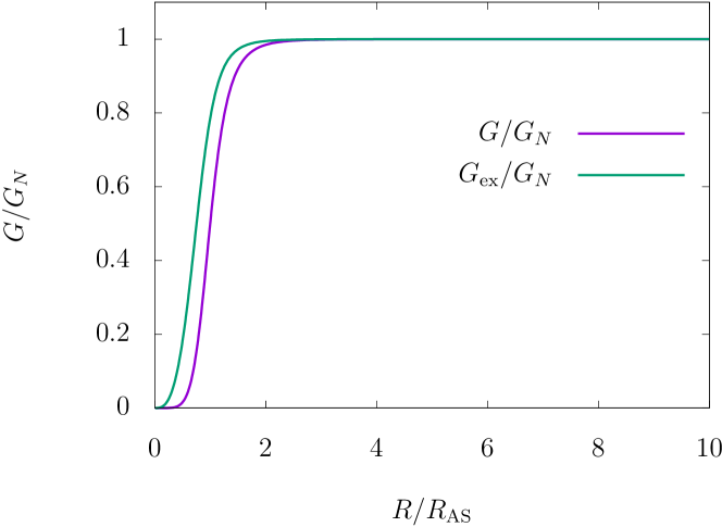
Figure 5: The effective gravitational constant $G$ and the gravitational constant $G_{\rm ex}$ for the exterior are plotted for $\alpha=2$ and for $w=0$.

It would be interesting to plot $f(R)$ for different parameter values. In this case, we can rewrite $f(R)$ as

$$f(R)=1-2\tilde{\Omega}^{-1}\left(\frac{R}{G_{N}M}\right)^{2}\arctan\left[\tilde{\Omega}\left(\frac{R}{G_{N}M}\right)^{-3}\right].$$ (65)

In Fig. 6, we show $f(R)$ for different values of $\tilde{\Omega}$ with the horizontal axis $R$ normalized by half the gravitational radius, $G_{N}M$. We can see that if we fix $M$, the larger the $\tilde{\omega}$ is, the stronger the modified effect becomes. So, $\tilde{\Omega}\simeq 1$ is the condition that divides a regular black hole and a gravastar. In fact, as seen in Fig. 6, the critical value $\tilde{\Omega}_{c}$ is numerically given as $\tilde{\Omega}\simeq 3.9$. Interestingly, the radius of the event horizon is fairly insensitive to the value of the quantum correction $\tilde{\Omega}$ as long as it has an event horizon or $\tilde{\Omega}$ is smaller than the critical value $\tilde{\Omega}_{c}$. Using $\tilde{\Omega}_{c}$, we can express the critical mass $M_{c}$ as

$$M_{c}=\sqrt{\frac{\tilde{\omega}^{1/\alpha}}{\frac{4\pi}{3}G_{N}\tilde{\Omega}_{c}}}=\sqrt{\frac{\tilde{\omega}^{1/\alpha}}{\frac{4\pi}{3}\tilde{\Omega}_{c}}}m_{P},$$ (66)

below which the black hole event horizon disappears.

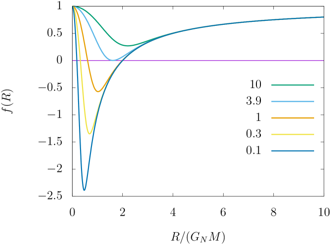
Figure 6: The function $f(R)$ for different values of $\tilde{\Omega}=\tilde{\omega}/[(4\pi/3)G_{N}M^{2}]$, where $\alpha=2$ and $w=0$ are fixed. Each curve is labeled with the value of $\tilde{\Omega}$. We can see that the critical value is given by $\tilde{\Omega}\simeq 3.9$.

V Discussion

V.1 Evaporation process of the regular black holes

For the regular black holes discussed above, we can calculate the Hawking temperature $T_{H}=\kappa/(2\pi)$, where

$$\kappa=\frac{f^{\prime}(R_{h+})}{2}$$ (67)

is the surface gravity at the event horizon $R=R_{h+}$. If we fix the theory parameters $\tilde{\omega}$ and $\alpha$ during semiclassical quasistatic evaporation, we expect that the mass of the black hole changes according to

$$\frac{dM}{dt}\simeq-4\pi R_{h+}^{2}\Gamma_{\rm eff}g_{\rm eff}\sigma T_{H}^{4},$$ (68)

where $\sigma=\pi^{2}/60$, $g_{\rm eff}$ and $\Gamma_{\rm eff}$ are the Stefan-Boltzmann constant, the effective degrees of freedom and the effective grey-body factor, respectively.

If the mass is large enough so that $M\gg M_{c}$, $T_{H}$ is approximately given by its Schwarzschild value $1/(8\pi M)$ and the evaporation time scale is given by $t_{\rm ev}\simeq G_{N}^{2}M^{3}/(\Gamma_{\rm eff}g_{\rm eff})$. So, the time evolution of $M$ is given by

$$M\simeq\left(1-\frac{t-t_{i}}{t_{\rm ev}}\right)^{1/3}M_{i},$$ (69)

where $M=M_{i}$ is the initial mass at $t=t_{i}$.

If the mass equals to a critical value $M_{c}$, the horizon becomes degenerate and the Hawking temperature vanishes, where $M_{c}$ is determined by the degeneracy or extremality condition $f(R_{h})=f^{\prime}(R_{h})=0$. Thus, as the mass decreases to a value very close to the critical one, the temperature quickly drops and the evaporation is strongly suppressed. We call this phase late-time evaporation.

To derive the behavior of the late-time evaporation, we explicitly write $f$ as a function of both $R$ and $M$, i.e., $f=f(R,M)$. Since $f=f_{,R}=0$ at $R=R_{c}$ and $M=M_{c}$, we can have the Taylor-series expansion of $f$ at $(R_{c},M_{c})$ as follows:

$$f(R,M)=f_{,M}(M-M_{c})+\frac{1}{2}f_{,RR}(R-R_{c})^{2}+f_{,RM}(R-R_{c})(M-M_{c})+\frac{1}{2}f_{,MM}(M-M_{c})^{2}+O(3),$$ (70)

where the derivatives are evaluated at $(R_{c},M_{c})$ and $O(3)$ denotes cubic and higher order terms in powers of $(R-R_{c})$ and $(M-M_{c})$. For $M\simeq M_{c}$ and $M>M_{c}$, we can find the outer and inner horizons $R=R_{h\pm}$ to the lowest order as follows:

$$R_{h\pm}\simeq R_{c}\pm\sqrt{-2f_{,M}(f_{,RR})^{-1}}(M-M_{c})^{1/2}.$$ (71)

Using Eqs. (67), (70) and (71), the surface gravity at the outer horizon is calculated to give

$$\kappa\simeq\sqrt{-\frac{1}{2}f_{,RR}f_{,M}}(M-M_{c})^{1/2}.$$ (72)

Equation (68) then can be integrated to give

$$M-M_{c}\simeq\frac{1}{C(t-t_{t})+(M_{t}-M_{c})^{-1}},$$ (73)

where

$$C=4\pi R_{c}^{2}\Gamma_{\rm eff}g_{\rm eff}\sigma\frac{(f_{,RR}f_{,M})^{2}}{4(2\pi)^{4}}=\frac{1}{480\pi}\Gamma_{\rm eff}g_{\rm eff}R_{c}^{2}(f_{,RR}f_{,M})^{2}$$ (74)

and the integration constant is fixed so that $M=M_{t}$ at the transition time $t=t_{t}$ to the late-time evaporation. The transition mass $M_{t}$ should be taken as a few times larger than the critical mass $M_{c}$.

Thus, after the mass decreases to $M_{t}$ in the early-time evaporation for the timescale $t_{\rm ev}$, the black hole undergoes a transition to the late-time evaporation, in which the mass asymptotically decreases towards $M_{c}$ and the temperature decreases in proportion to $t^{-1/2}$ for infinitely long time $t\to\infty$. We can also conclude that neither regular extremal black holes nor gravastars can be obtained as final outcomes of Hawking evaporation in finite time.

It is clear that the above discussion is too simplified and in reality the transition should occur continuously. We should also note that other possible quantum gravity effects are neglected. Further details of the evaporation process will be presented elsewhere Harada et al. (2025).

V.2 Interpretation of the exterior metric

We should be cautioned that the exterior metric obtained here is neither a vacuum solution nor perfect fluid solution in general. In particular, this is not a solution of the effective action given by Eq. (6). This is an inevitable consequence of the assumption of smooth matching with the static exterior with the metric in the form of Eq. (47). We can interpret this as that the action (6) that only admits perfect fluid is adequate to describe the homogeneous and isotropic interior but inadequate to describe the exterior region. From this point of view, we should construct an effective action which can also deal with matter fields that cannot be described by perfect fluid. Alternatively, we might still seek for a static exterior metric containing only perfect fluid governed by the action (6), for which we have to give up the metric form (47). We can also infer that the assumptions of homogeneous interior and/or smooth matching and/or static exterior must be broken. In fact, even in standard gravitational collapse in GR, it is well-known that smooth matching between the homogeneous interior and the vacuum exterior can be compatible only with a pressure-free fluid, or dust. Furthermore, if we assume vacuum, it seems that the action 6 will not give any quantum correction. We leave these problems open for future studies.

VI Conclusion

Asymptotically safe gravity is a nonperturbatively renormalizable theory of gravity, characterized by an RG flow with a fixed point at which the dimensionless coupling constants take nonvanishing finite values as the cut-off scale increases.

Inspired by this idea, we have analyzed the gravitational collapse of a uniform ball of perfect fluid within an effective action framework, where the effective gravitational constant and cosmological constant are functions of the energy density, as proposed by Markov and Mukhanov. We have parameterized the effective gravitational constant $G(\epsilon)$ in terms of $\alpha$ and $\tilde{\omega}$ such that $G(\epsilon)\to G_{N}$ as $\epsilon\to 0$ and $\epsilon^{\alpha}G(\epsilon)$ approaches a nonzero finite value as $\epsilon\to\infty$.

We have shown that only for $\alpha>1$, the effective cosmological constant $\Lambda(\epsilon)$ really approaches constant and dominates the bare matter field as $\epsilon\to\infty$. Our findings indicate that singularity formation is completely avoided for $\alpha>1$, regardless of the initial conditions, whereas for $1/2<\alpha\leq 1$, singularity avoidance is only partial, with singularities inevitably forming in the gravitationally unbound case. In contrast, for $0<\alpha<1/2$, the dimensionless cosmological constant diverges as $\epsilon\to\infty$, rendering the scenario inconsistent with asymptotic safety. Moreover, in the marginal case $\alpha=1$, although singularity formation remains unavoidable in unbounded collapse, its curvature strength is significantly weakened due to quantum gravity effects.

By smoothly matching the collapsing interior to the static exterior, we have successfully constructed a spacetime that describes the formation of both a regular black hole and a continuous gravastar, each possessing a de Sitter core at the center for $\alpha>1$ and $K\leq 0$, while for $K>0$, the core remains uniform.

The implications of our results are multifold. Firstly, if singularity resolution is a necessary feature of asymptotically safe gravity, then within the Markov-Mukhanov effective action framework, the effective gravitational constant must behave as in the case of $\alpha>1$. The decrease in the effective gravitational constant for $0<\alpha\leq 1$ is insufficient to fully resolve singularities, imposing a strong constraint on singularity resolution phenomenology.

Secondly, our study provides a concrete example of a formation scenario for regular black holes and gravastars driven by quantum gravity effects within asymptotically safe gravity. In particular, it is noteworthy that our findings demonstrate the emergence of a de Sitter core as a natural outcome of singularity-free gravitational collapse. In the present setting, for gravitationally unbound collapse or for cases with negative spatial curvature, this mechanism is the only means of preventing singularity formation.

Thirdly, this phenomenon has potential applications to very small black holes that may have formed in the early Universe, known as primordial black holes. For a comprehensive review of primordial black holes and related references, see Ref. Byrnes et al. (2025). Since primordial black holes can form at extremely high energy densities and with very small masses, they are more likely to be affected by quantum gravity effects than standard astrophysical black holes. Investigating how the quantum effects studied in this paper influence primordial black hole formation would be of great interest.

Finally, we speculate that nearly extremal regular black holes in the late stages of Hawking evaporation, with temperatures approaching zero, may play a significant role in dark matter models.

Appendix A (Non-)conservation of the bare matter field

A.1 Non-conservation of the bare matter field

Let us first review the construction of the action for an isentropic perfect fluid following Ref. Hawking and Ellis (2023). An isentropic perfect fluid is introduced with a congruence of timelike curves, which is called a fluid flow, and a number density. We denote the tangent vector of the fluid flow and the number density by $W^{\mu}$ and $n$, respectively. We define a normalized tangent vector along the fluid flow

$$u^{\mu}=\frac{W^{\mu}}{\sqrt{-g_{\alpha\beta}W^{\alpha}W^{\beta}}}$$ (75)

and require that $j^{\mu}=nu^{\mu}$ satisfies the conservation law

$$\nabla_{\mu}j^{\mu}=0.$$ (76)

For the action given by Eq. (1), we assume that $\epsilon$ is a function of $n$. Varying the fluid action with respect to the fluid flow $W^{\mu}$ keeping $j^{\mu}$ conserved, we obtain the Euler equation

$$(\epsilon+p)u^{\nu}\nabla_{\nu}u^{\mu}=-(g^{\mu\nu}+u^{\mu}u^{\nu})\nabla_{\nu}p,$$ (77)

where $p$ is given by Eq. (2). The number conservation (76) can be rewritten in terms of $\epsilon$ and $p$ as

$$u^{\mu}\nabla_{\mu}\epsilon+(\epsilon+p)\nabla_{\mu}u^{\mu}=0,$$ (78)

which is interpreted as the energy conservation. We can derive the stress-energy tensor by the variation of the fluid action with respect to the metric $g_{\mu\nu}$ keeping $j^{\mu}$ conserved. The resulting form of the stress-energy tensor is given by Eq. (4). Now the conservation law (5) follows from the invariance of the action against the infinitesimal coordinate transformation. This is equivalent to (77) and (78). For a given metric and an EOS, we can obtain a solution of these matter equations in terms of $u^{\mu}$ and $\epsilon$. We can obtain $n$ by directly solving the number conservation (76).

Let us move onto the Markov-Mukhanov action (6), where the matter term $16\pi G_{N}\epsilon$ is replaced by $2\chi(\epsilon_{B})\epsilon_{B}$, where ”B” is put in this section to distinguish it from the quantities in the original classical system. We can rewrite Eq. (12) as

$$8\pi G_{N}T^{\mu\nu}_{\rm eff}=8\pi G(\epsilon_{B}(n_{\rm eff}))\tilde{T}^{\mu\nu}_{B}-\Lambda(\epsilon_{B}(n_{\rm eff}))g^{\mu\nu},$$ (79)

$$\tilde{T}^{\mu\nu}_{B}:=[\epsilon_{B}(n_{\rm eff})+p_{B}(n_{\rm eff})]u_{\rm eff}^{\mu}u_{\rm eff}^{\nu}+p_{B}(n_{\rm eff})g^{\mu\nu},$$ (80)

where $n_{\rm eff}$ and $u_{\rm eff}^{\mu}$ are the conserved number density and the unit fluid four-velocity associated with the effective fluid. Since the effective and bare fluids follow different EOS’s in general as we have seen in Sec. II.1, the solutions $u^{\mu}$ of the Euler equation are different from each other in general. This is obvious if we are reminded that fluids following different EOS’s will have different propagation speeds of sound waves in general. For the solution $u_{\rm eff}^{\mu}$ of the Euler equation for the effective fluid, we can calculate $n_{\rm eff}$ and then $\epsilon_{B}(n_{\rm eff})$ and $p_{B}(n_{\rm eff})$. However, thus constructed $\tilde{T}_{B}^{\mu\nu}$ given by Eq. (80) cannot satisfy the conservation law in general.

On the other hand, if we require the conservation law for the bare fluid

$$T_{B}^{\mu\nu}=[\epsilon_{B}(n_{B})+p_{B}(n_{B})]u_{B}^{\mu}u_{B}^{\nu}+p_{B}(n_{B})g^{\mu\nu},$$ (81)

we need to realize that the solution $u_{B}^{\mu}$ that satisfies the Euler equation for the bare fluid is different from $u_{\rm eff}$ in general. So, we have to distinguish between $u^{\mu}_{B}$ and $u^{\mu}_{\rm eff}$ and therefore the conserved number densities $n_{B}$ and $n_{\rm eff}$. Thus, we can obtain the bare stress-energy tensor (81), which trivially is conserved by construction. However, if we are given the modified action (6) only, we have no strong reason to define the conserved bare stress-energy tensor $T_{B}^{\mu\nu}$ given by Eq. (81).

A.2 Conservation of the bare matter field in the FLRW spacetime

Here, we apply the Markov-Mukhanov action to the FLRW spacetime. Since this spacetime has high symmetry, we need great care for the application of the discussion in the previous subsection. In the FLRW spacetime with the metric (20), it is clear that the conservation of the effective stress-energy tensor (16), or more precisely, the Euler equation admits a trivial solution

$$u_{\rm eff}^{\mu}=\left(\frac{\partial}{\partial\tau}\right)^{\mu}.$$ (82)

The conservation of $j^{\mu}=n_{\rm eff}u_{\rm eff}^{\mu}$ yields

$$n_{\rm eff}\propto\frac{1}{a^{3}}.$$ (83)

Then, we can calculate $\epsilon_{\rm eff}=\epsilon_{\rm eff}(n_{\rm eff})$ and $p_{\rm eff}=p_{\rm eff}(n_{\rm eff})$ and construct $T_{\rm eff}^{\mu\nu}$. We can understand that $\nabla_{\mu}T_{\rm eff}^{\mu\nu}=0$ is satisfied from the discussion in the previous subsection.

We should notice, however, that the solution (82) does not depend on the EOS. This means that although the bare fluid follows another EOS than the effective one, both the bare and effective fluids share the same solution (82) and (83), i.e., $u^{\mu}_{\rm eff}=u_{B}$ and $n_{\rm eff}=u_{B}$. In other words, using the same $u_{\rm eff}^{\mu}$ and $n_{\rm eff}$, we can find that $\tilde{T}^{\mu\nu}_{B}$ defined by Eq. (80) satisfies the conservation law

$$\nabla_{\mu}\tilde{T}^{\mu\nu}_{B}=0.$$ (84)

This is completely due to high symmetry of the FLRW spacetime and therefore accidenta in this sense. This coincidence occurs if the fluid flow $u^{\mu}_{B}$ determined by $\nabla_{\mu}T_{B}^{\mu\nu}=0$ coincides with $u^{\mu}_{\rm eff}$ determined by $\nabla_{\mu}T_{\rm eff}^{\mu\nu}=0$, in other words, when $u^{\mu}_{B}=u^{\mu}_{\rm eff}$ holds.

Appendix B Case of $\alpha=1/2$ and $w=1/3$

The case $\alpha=1/2$ and $w=1/3$ seems to be well motivated for a simplistic dimensional argument might imply $\alpha=1/2$ as discussed in Sec. II.2 and matter fields with asymptotic freedom should behave like radiation at high-energy limit. In this case, we obtain

$$V(a) = -\frac{8\pi G_{N}^{-1}}{3}a^{2}2\tilde{\omega}^{-2}\left[\tilde{\omega}\sqrt{G_{N}^{2}\epsilon}-\ln(1+\tilde{\omega}\sqrt{G_{N}^{2}\epsilon})\right],$$ (85)

$$G_{N}^{2}\epsilon_{\rm eff} = 2\tilde{\omega}^{-2}\left[\tilde{\omega}\sqrt{G_{N}^{2}\epsilon}-\ln(1+\tilde{\omega}\sqrt{G_{N}^{2}\epsilon})\right],$$ (86)

$$\Lambda = 8\pi G_{N}^{-1}\tilde{\omega}^{-2}\left\{2\left[\tilde{\omega}\sqrt{G_{N}^{2}\epsilon}-\ln(1+\tilde{\omega}\sqrt{G_{N}^{2}\epsilon})\right]-\tilde{\omega}^{2}\frac{G_{N}^{2}\epsilon}{1+\tilde{\omega}\sqrt{G_{N}^{2}\epsilon}}\right\}.$$ (87)

The dimensionless cosmological constant is given by

$$\lambda(k)=\frac{8\pi\omega}{\tilde{\omega}^{2}}\left\{2\left[1-\frac{\ln(1+\tilde{\omega}\sqrt{G_{N}^{2}\epsilon})}{\tilde{\omega}\sqrt{G_{N}^{2}\epsilon}}\right]-\frac{\tilde{\omega}\sqrt{G_{N}^{2}\epsilon}}{1+\tilde{\omega}\sqrt{G_{N}^{2}\epsilon}}\right\}.$$ (88)

As $\epsilon$ increases from $0$ to $\infty$, this monotonically increase from $0$ to ${8\pi\omega}/({\tilde{\omega}^{2}})$. Thus, $\lambda(k)$ is kept finite in the limit $\epsilon\to\infty$.

Since $\epsilon=\epsilon_{1}/a^{4}$, we find $\epsilon_{\rm eff}\to\infty$ in the limit of $a\to 0$. We can find that $V(a)$ is a monotonically increasing function with $V(0)=V_{0}$, where

$$V_{0}=-\frac{8\pi G_{N}^{-1}}{3}2\tilde{\omega}^{-1}\sqrt{G_{N}^{2}\epsilon_{1}}$$ (89)

and $V(a)\to 0$ as $a\to\infty$. Therefore, $K>-V_{0}$ is prohibited. For $K=-V_{0}$, we cannot set a regular initial condition because only $a=0$ is allowed. For $K<-V_{0}$, the collapse encounters singularity in finite proper time. So, there is no singularity resolution. The collapse encounters singularity in finite proper time for $K<-V_{0}$. The shape of $V(a)$ for $\alpha=1/2$ and $w=1/3$ is plotted by a cyan curve in Fig. 1.

Appendix C Junction conditions

In this section, we implement the matching between the interior and exterior regions following Ref. Poisson (2009). We use the coordinates $x^{\alpha}$ for the 4-dimensional spacetime ${\cal M}$ and $y^{a}$ for the 3-dimensional timelike or spacelike hypersurface $\Sigma$, which is given by $\ell(x^{\alpha})=0$. We define the unit normal vector $n^{\alpha}$ to $\Sigma$ and the induced metric $h_{ab}$ and the extrinsic curvature $K_{ab}$ on $\Sigma$ as

$$n_{\alpha} = \frac{\epsilon\partial_{\alpha}\ell}{\sqrt{|\partial_{\alpha}\ell\partial^{\alpha}\ell|}};\quad n^{\alpha}n_{\alpha}=\epsilon=\pm 1,$$

$$e^{\alpha}_{a} = \frac{\partial x^{\alpha}}{\partial y^{a}},~~h_{ab}=g_{\alpha\beta}e^{\alpha}_{a}e^{\beta}_{b},~~K_{ab}=n_{(\alpha;\beta)}e^{\alpha}_{a}e^{\beta}_{b}.$$ (90)

We denote the spacetime regions divided by $\Sigma$ with ${\cal M}_{\pm}$.

We assume that the interior region ${\cal M}_{-}$ is with the FLRW metric given by Eq. (20) and the exterior ${\cal M}_{+}$ is with the general static spherically symmetric metric

$$ds^{2}=-e^{\nu(R)}dt^{2}+e^{\lambda(R)}dR^{2}+R^{2}d\Omega^{2}.$$ (91)

The junction hypersurface $\Sigma$ is written by $r=r_{b}$ in ${\cal M}_{-}$ and $t=T_{b}(\tau)$ and $R=R_{b}(\tau)$ in ${\cal M}_{+}$, where $\tau$ is the proper time. We choose $y^{a}=(\tau,\theta,\phi)$.

In ${\cal M}_{-}$, we have

$$n^{-}_{\alpha} = \frac{a}{\sqrt{1-Kr_{b}^{2}}}(0,1,0,0),~~e^{-\alpha}_{0}=(1,0,0,0),~~e^{-\alpha}_{2}=(0,0,1,0),~~e^{-\alpha}_{3}=(0,0,0,1),$$

$$h^{-}_{ab} = \mbox{diag}(-1,(ar_{b})^{2},(ar_{b})^{2}\sin^{2}\theta),$$ (92)

and the nonvanishing components of the extrinsic curvature on $\Sigma$ is given by

$$K^{-}_{00}=0,~~K^{-}_{22}=ar_{b}\sqrt{1-Kr_{b}^{2}},~~K^{-}_{33}=ar_{b}\sin^{2}\theta\sqrt{1-Kr_{b}^{2}}.$$ (93)

In ${\cal M}_{+}$, we have

$$n^{+}_{\alpha} = Ne^{(\nu+\lambda)/2}(-\dot{R}_{b},\dot{T}_{b},0,0),~~e^{+\alpha}_{0}=(\dot{T}_{b},\dot{R}_{b},0,0),~~e^{+\alpha}_{2}=(0,0,1,0),~~e^{+\alpha}_{3}=(0,0,0,1),$$

$$h^{+}_{ab} = \mbox{diag}(-e^{\nu}\dot{T}_{b}^{2}+e^{\lambda}\dot{R}_{b}^{2},R_{b}^{2},R_{b}^{2}\sin^{2}\theta),$$ (94)

where the dot denotes the ordinary derivative with respect to $\tau$ and $N$ is a normalisation factor.

The continuity of the first fundamental form $[h_{ab}]=0$ requires

$$-e^{\nu}\dot{T}_{b}^{2}+e^{\lambda}\dot{R}_{b}^{2}=-1,$$ (95)

$$R_{b}=ar_{b}.$$ (96)

Then, Eq. (95) fixes the normalisation constant to $N=1$.

Using the nonvanishing independent components of the Christoffel symbols in ${\cal M}_{+}$,

$$\Gamma^{0}_{01} = \frac{\nu^{\prime}}{2},~~\Gamma^{1}_{00}=\frac{1}{2}e^{\nu-\lambda}\nu^{\prime},\quad\Gamma^{1}_{11}=\frac{\lambda^{\prime}}{2},\quad\Gamma^{1}_{22}=-Re^{-\lambda},\quad\Gamma^{1}_{33}=-Re^{-\lambda}\sin^{2}\theta$$

$$\Gamma^{2}_{12} = \frac{1}{R},\quad\Gamma^{2}_{33}=-\sin\theta\cos\theta,\quad\Gamma^{3}_{13}=\frac{1}{R},\quad\Gamma^{3}_{23}=\cot\theta,$$ (97)

we obtain the nonvanishing components of the extrinsic curvature

$$K^{+}_{00} = e^{(\nu+\lambda)/2}(-\ddot{R}_{b}\dot{T}_{b}+\dot{R}_{b}\ddot{T}_{b})+\frac{1}{2}e^{(\nu-\lambda)/2}[(\nu^{\prime}-\lambda^{\prime})e^{\lambda}\dot{R}_{b}^{2}-\nu^{\prime}]\dot{T}_{b},$$

$$K^{+}_{22} = R_{b}e^{(\nu-\lambda)/2}\dot{T}_{b},~~K^{+}_{33}=R_{b}e^{(\nu-\lambda)/2}\dot{T}_{b}\sin^{2}\theta.$$ (98)

Using Eqs. (95) and (96) under the assumption $e^{\nu}=f$ and $e^{\lambda}=1/f$, we can find that $K_{00}^{+}$ takes a particularly simple form as

$$K^{+}_{00}=-\frac{2\ddot{R}_{b}+f^{\prime}}{2f\dot{T}_{b}},~~K^{+}_{22}=Rf\dot{T}_{b},~~K^{+}_{33}=Rf\dot{T}_{b}\sin^{2}\theta,$$ (99)

where $\dot{T}_{b}$ is given by

$$\dot{T}_{b}=\frac{\sqrt{\dot{R}_{b}^{2}+f}}{f}.$$ (100)

The continuity of the second fundamental form $[K_{ab}]=0$ together with the above equations requires

$$2\ddot{R}_{b}+f^{\prime} = 0,$$ (101)

$$R_{b}\sqrt{\dot{R}_{b}^{2}+f} = ar_{b}\sqrt{1-Kr_{b}^{2}}.$$ (102)

From Eq. (102) together with Eq. (96), we find

$$\dot{R}_{b}^{2}+f=1-Kr_{b}^{2}.$$ (103)

Differentiating this with respect to $\tau$ gives Eq. (101). From Eq. (103) with Eq. (48), we can derive

$$\dot{a}^{2}-\frac{2G_{N}m(ar_{b})}{ar_{b}^{3}}+K=0.$$ (104)

This is consistent with the Einstein equation in the interior, which is Eq. (21), if and only if

$$m(ar_{b})=\frac{4\pi}{3}(ar_{b})^{3}\epsilon_{\rm eff}(a)$$ (105)

or

$$m(R_{b})=\frac{4\pi}{3}R_{b}^{3}\epsilon_{\rm eff}\left(\frac{R_{b}}{r_{b}}\right).$$ (106)

Thus, the second junction condition determines the function $m(R)$. This is equivalent to the continuity of the Misner-Sharp mass at the junction hypersurface $\Sigma$.

References

- Reuter (1998) M. Reuter, Phys. Rev. D 57, 971 (1998), arXiv:hep-th/9605030 .
- Souma (1999) W. Souma, Progress of Theoretical Physics 102, 181 (1999), https://academic.oup.com/ptp/article-pdf/102/1/181/19571317/102-1-181.pdf .
- Percacci (2017) R. Percacci, An Introduction to Covariant Quantum Gravity and Asymptotic Safety (World Scientific, 2017) https://www.worldscientific.com/doi/pdf/10.1142/10369 .
- Reuter and Saueressig (2018) M. Reuter and F. Saueressig, Quantum Gravity and the Functional Renormalization Group: The Road towards Asymptotic Safety (2018).
- Weinberg (1980) S. Weinberg, “ULTRAVIOLET DIVERGENCES IN QUANTUM THEORIES OF GRAVITATION,” in General Relativity: An Einstein Centenary Survey (1980) pp. 790–831.
- Penrose (1965) R. Penrose, Phys. Rev. Lett. 14, 57 (1965).
- Hawking and Penrose (1970) S. W. Hawking and R. Penrose, Proc. Roy. Soc. Lond. A 314, 529 (1970).
- Hawking and Ellis (2023) S. W. Hawking and G. F. R. Ellis, The Large Scale Structure of Space-Time, Cambridge Monographs on Mathematical Physics (Cambridge University Press, 2023).
- Wald (1984) R. M. Wald, General Relativity (Chicago Univ. Pr., Chicago, USA, 1984).
- Bardeen (1968) J. Bardeen, in Proceedings of the 5th International Conference on Gravitation and the Theory of Relativity, p. 87, Sept., 1968. (1968).
- Hayward (2006) S. A. Hayward, Phys. Rev. Lett. 96, 031103 (2006), arXiv:gr-qc/0506126 .
- Maeda (2022) H. Maeda, JHEP 11, 108 (2022), arXiv:2107.04791 [gr-qc] .
- Bonanno et al. (2017) A. Bonanno, B. Koch, and A. Platania, Class. Quant. Grav. 34, 095012 (2017), arXiv:1610.05299 [gr-qc] .
- Chen et al. (2022) C.-M. Chen, Y. Chen, A. Ishibashi, N. Ohta, and D. Yamaguchi, Phys. Rev. D 105, 106026 (2022), arXiv:2204.09892 [hep-th] .
- Chen et al. (2024) C.-M. Chen, Y. Chen, A. Ishibashi, and N. Ohta, Chin. J. Phys. 92, 766 (2024), arXiv:2308.16356 [hep-th] .
- Chen et al. (2023) C.-M. Chen, Y. Chen, A. Ishibashi, and N. Ohta, Class. Quant. Grav. 40, 215007 (2023), arXiv:2303.04304 [hep-th] .
- Mazur and Mottola (2004) P. O. Mazur and E. Mottola, Proc. Nat. Acad. Sci. 101, 9545 (2004), arXiv:gr-qc/0407075 .
- Visser and Wiltshire (2004) M. Visser and D. L. Wiltshire, Class. Quant. Grav. 21, 1135 (2004), arXiv:gr-qc/0310107 .
- Ogawa and Ishihara (2023) T. Ogawa and H. Ishihara, Phys. Rev. D 107, L121501 (2023), arXiv:2303.07632 [hep-th] .
- Ogawa and Ishihara (2024) T. Ogawa and H. Ishihara, Phys. Rev. D 110, 124003 (2024), arXiv:2409.07818 [hep-th] .
- Reuter and Weyer (2004) M. Reuter and H. Weyer, Phys. Rev. D 69, 104022 (2004).
- Markov and Mukhanov (1984) M. A. Markov and V. F. Mukhanov, JETP Lett. 40, 1043 (1984).
- Bonanno et al. (2024) A. Bonanno, D. Malafarina, and A. Panassiti, Phys. Rev. Lett. 132, 031401 (2024), arXiv:2308.10890 [gr-qc] .
- Zholdasbek et al. (2024) A. Zholdasbek, H. Chakrabarty, D. Malafarina, and A. Bonanno, (2024), arXiv:2405.02636 [gr-qc] .
- Bueno et al. (2024a) P. Bueno, P. A. Cano, R. A. Hennigar, and A. J. Murcia, (2024a), arXiv:2412.02742 [gr-qc] .
- Bueno et al. (2024b) P. Bueno, P. A. Cano, R. A. Hennigar, and A. J. Murcia, (2024b), arXiv:2412.02740 [gr-qc] .
- Bonanno and Reuter (2000) A. Bonanno and M. Reuter, Phys. Rev. D 62, 043008 (2000), arXiv:hep-th/0002196 .
- Starobinsky (1982) A. A. Starobinsky, Phys. Lett. B 117, 175 (1982).
- Starobinsky (1986) A. A. Starobinsky, Lect. Notes Phys. 246, 107 (1986).
- Harada et al. (2018) T. Harada, B. J. Carr, and T. Igata, Class. Quant. Grav. 35, 105011 (2018), arXiv:1801.01966 [gr-qc] .
- Harada et al. (2022) T. Harada, T. Igata, T. Sato, and B. Carr, Class. Quant. Grav. 39, 145008 (2022), arXiv:2110.13421 [gr-qc] .
- Sato and Kodama (1992) H. Sato and H. Kodama, Ippansoutaiseiriron (In Japanese) (Iwanami Shoten, Publishers, Tokyo, Japan, 1992).
- Griffiths and Podolsky (2009) J. B. Griffiths and J. Podolsky, Exact Space-Times in Einstein’s General Relativity, Cambridge Monographs on Mathematical Physics (Cambridge University Press, Cambridge, 2009).
- Clarke (1994) C. J. S. Clarke, The Analysis of space-time singularities, Cambridge Lecture Notes in Physics (Cambridge Univ. Press, Cambridge, UK, 1994).
- Harada et al. (2025) T. Harada, C.-M. Chen, and R. Mandal, in preparation (2025).
- Byrnes et al. (2025) C. Byrnes, G. Franciolini, T. Harada, P. Pani, and M. Sasaki, eds., Primordial Black Holes, Springer Series in Astrophysics and Cosmology (Springer, 2025).
- Poisson (2009) E. Poisson, A Relativist’s Toolkit: The Mathematics of Black-Hole Mechanics (Cambridge University Press, 2009).