Exact Learning of Permutations for Nonzero Binary Inputs with Logarithmic Training Size and Quadratic Ensemble Complexity

Abstract

The ability of an architecture to realize permutations is quite fundamental. For example, Large Language Models need to be able to correctly copy (and perhaps rearrange) parts of the input prompt into the output. Classical universal approximation theorems guarantee the existence of parameter configurations that solve this task but offer no insights into whether gradient-based algorithms can find them. In this paper, we address this gap by focusing on two-layer fully connected feed-forward neural networks and the task of learning permutations on nonzero binary inputs. We show that in the infinite width Neural Tangent Kernel (NTK) regime, an ensemble of such networks independently trained with gradient descent on only the $k$ standard basis vectors out of $2^{k}-1$ possible inputs successfully learns any fixed permutation of length $k$ with arbitrarily high probability. By analyzing the exact training dynamics, we prove that the network’s output converges to a Gaussian process whose mean captures the ground truth permutation via sign-based features. We then demonstrate how averaging these runs (an “ensemble” method) and applying a simple rounding step yields an arbitrarily accurate prediction on any possible input unseen during training. Notably, the number of models needed to achieve exact learning with high probability (which we refer to as ensemble complexity) exhibits a linearithmic dependence on the input size $k$ for a single test input and a quadratic dependence when considering all test inputs simultaneously.

1 Introduction

Neural networks have long been known as universal function approximators: a two-layer feed-forward neural network with sufficient width can approximate any continuous function on a compact domain (Cybenko, 1989; Hornik et al., 1989). However, these classical theorems only guarantee the existence of a suitable parameter configuration; they do not explain whether a standard training procedure (e.g., gradient-based training) can efficiently discover such parameters. While universal approximation highlights the expressive power of neural networks, it does not directly address how trained networks generalize beyond the specific data they observe.

In contrast, the literature on domain generalization provides general learning guarantees from a Probably Approximately Correct (PAC) learning perspective. Given training and testing distributions, one can bound the expected test loss of any hypothesis that minimizes the empirical training risk. This bound typically depends on the discrepancy between the training and testing distributions, the training sample size, and the complexity of the hypothesis class (Ben-David et al., 2006; Mansour et al., 2009). However, such bounds do not account for training dynamics, making them quite pessimistic, especially when a single hypothesis that fails to perform well on the testing data is a minimizer of the training loss, even if a standard training procedure would never find it.

Our work complements these approaches in a more specialized setting. We focus on exact learning using the training dynamics of a simple two-layer network in the infinite-width Neural Tangent Kernel (NTK) regime. We show that an ensemble of such models can learn with arbitrarily high probability a global transformation, in our case, a permutation function, from a logarithmically small training set.

Contributions.

We use the NTK framework to analyze the problem of learning permutations, a task many models need to perform as a subroutine, yet it is unknown if it can be performed exactly with high probability. We list our contributions below:

• We show that when the inputs are nonzero, normalized, and binary, a two-layer fully connected feed-forward network in the infinite width limit trained on the standard basis using gradient descent (or gradient flow) converges to a Gaussian Process whose mean captures the ground truth permutation via sign-based features. More precisely, each entry in the predicted mean is non-positive exactly when (and only when) the corresponding ground-truth value is zero.

• We show that this can be achieved with logarithmic training size by picking the training set to consist of the $k$ standard basis vectors (out of the $2^{k}-1$ vectors in the domain), where $k$ is the input length.

• We can achieve zero error on any input unseen during training, with high probability, by averaging the output of $\mathcal{O}(k\log k)$ independently trained models and applying a post-processing rounding step. To guarantee zero error simultaneously for all inputs, the same procedure requires averaging the output of $\mathcal{O}(k^{2})$ independently trained models.

2 Literature Review

The NTK framework (Jacot et al., 2018) is a popular framework designed to provide insights into the continuous-time gradient descent (gradient flow) dynamics of fully connected feed-forward neural networks with widths tending to infinity. The initial results have been extended to discrete gradient descent (Lee et al., 2019) as well as generalized to more architecture families like RNNs and Transformers (Yang, 2020; Yang and Littwin, 2021). While the general NTK theory has been extensively studied, very few works use the framework to study the performance of neural architectures on specific tasks. Notably, the framework has been used to attempt to explain the “double descent” phenomenon (Nakkiran et al., 2020) observed in deep architectures (Adlam and Pennington, 2020; Singh et al., 2022). It has also been used to study the behavior of Residual Networks (Yuqing et al., 2022) and Physics-Informed Neural Networks (Wang et al., 2022). To the best of our knowledge, the closest work to ours is Boix-Adserà et al. (2024), where the authors use results from the general NTK theory to prove that Transformers can provably generalize out-of-distribution on template matching tasks. Furthermore, they show that feed-forward neural networks fail to generalize to unseen symbols for any template task, including copying, a special case of a permutation learning setting. In our paper, we show that feed-forward neural networks can indeed learn to copy without error with high probability. At first, this might seem to contradict Boix-Adserà et al. (2024). However, the key difference between our work and the work in Boix-Adserà et al. (2024) lies in the problem setting. The setting in Boix-Adserà et al. (2024) poses no restrictions to the input, whereas we require binary encoded input. Therefore, the model has access to all symbols during training. In particular, we specifically choose the training set, i.e. the standard basis, so that each symbol appears in every position. The restrictions above are what enable exact permutation learning.

Lastly, various studies highlight the expressive power of neural networks through simulation results. For instance, Siegelmann and Sontag (1995) demonstrates the Turing completeness of recurrent neural networks (RNNs), while Hertrich and Skutella (2023) introduces specific RNN constructions capable of solving the shortest paths problem and approximating solutions to the knapsack problem. Moreover, other simulation studies on Transformers have established their Turing completeness (Pérez et al., 2021; Wei et al., 2022) and showcased constructive solutions for linear algebra, graph-related problems (Giannou et al., 2023; Back De Luca and Fountoulakis, 2024; Yang et al., 2024), and parallel computation (Back de Luca et al., 2025). However, the results in these works are existential, and none considers the dynamics of the training procedure.

3 Notation and Preliminaries

Throughout the text, we use boldface to denote vectors. We reserve the notation $\bm{e_{1}},\bm{e_{2}},\dots$ for the standard basis vectors. We use $\bm{1}$ to denote the vector of all ones. For a vector $\bm{x}\in\mathbb{R}^{n}$ we denote by $\|\bm{x}\|:=\sqrt{\sum_{i=1}^{n}\bm{x}_{i}^{2}}$ the Euclidean norm of $\bm{x}$. We denote the $n\times n$ identity matrix by $I_{n}$. For $n\in\mathbb{N}:=\{1,2,\dots\}$ let

$$H_{n}=\{\bm{x}\in\mathbb{R}^{n}:\bm{x}_{i}=0\text{ or }\bm{x}_{i}=1\;\forall\,i=1,2,\dots,n\}$$

denote the $n$-dimensional Hamming cube (the set of all $n$-dimensional binary vectors). We use the notation $[n]$ to refer to the set $\{1,2,\dots,n\}$. For two matrices $A_{1}\in\mathbb{R}^{n_{1}\times m_{1}}$, $A_{2}\in\mathbb{R}^{n_{2}\times m_{2}}$ we denote by $A_{1}\otimes A_{2}\in\mathbb{R}^{n_{1}n_{2}\times m_{1}m_{2}}$ their Kronecker product. It is relatively easy to show that when $A$ and $B$ are square matrices (i.e. $n_{1}=m_{1}$ and $n_{2}=m_{2}$), the eigenvalues of $A_{1}\otimes A_{2}$ are given exactly by the products of the eigenvalues of $A_{1}$ and $A_{2}$. In particular, $A_{1}\otimes A_{2}$ is positive definite if $A_{1}$ and $A_{2}$ are positive definite.

3.1 Permutation matrices

A permutation matrix is a square binary matrix $P\in\{0,1\}^{n\times n}$ with exactly one entry of $1$ in each row and column. Let $\text{Sym}([n])$ denote the set of all permutations of the set $[n]$. Every permutation matrix can be mapped uniquely to a permutation $\pi\in\text{Sym}([n])$ formed by taking

$$\pi(i)=\text{the unique index }j\text{ such that }P_{i,j}=1$$

Multiplying a vector $\bm{v}\in\mathbb{R}^{n}$ with $P$ from the left corresponds to permuting the entries of $v$ according to $\pi$, that is $(P\bm{v})_{i}=\bm{v}_{\pi^{-1}(i)}$. We say that a neural network has learned a permutation $P$ if on input $\mathbf{v}$ it outputs $P\bm{v}$. When $P$ is the identity matrix the neural network simply copies the input.

3.2 NTK Results

In what follows, we provide a brief overview of the necessary theory used to derive our results. We refer the reader to Golikov et al. (2022) for a comprehensive treatment of the NTK theory.

3.2.1 General Architecture Setup

We follow the notation of Lee et al. 2019, which is, for the most part, consistent with the rest of the NTK literature. Let $\mathcal{D}\in\mathbb{R}^{n_{0}}\times\mathbb{R}^{k}$ denote the training set, $\mathcal{X}=\{x:(x,y)\in\mathcal{D}\}$ and $\mathcal{Y}=\{y:(x,y)\in\mathcal{D}\}$. The architecture is a fully connected feed-forward network with $L$ hidden layers with widths $n_{l}$, for $l=1,2,\dots,L$ and a readout layer with $n_{L+1}=k$. In our case, we consider networks with $L=1$ hidden layers. For each $\bm{x}\in\mathbb{R}^{n_{0}}$, we use $h^{l}(\bm{x}),x^{l}(\bm{x})\in\mathbb{R}^{n_{l}}$ to represent the pre- and post-activation functions at layer $l$ with input $\bm{x}$. The recurrence relation for a feed-forward network is given for $l=1,2,\dots,L+1$ by:

$$\left\{\begin{array}[]{ l }{h^{l}=W^{l}\bm{x}^{l-1}+b^{l}}\\ {\bm{x}^{l}=\phi(h^{l})}\end{array}\quad\text{ and }\quad\left\{\begin{array}[]{ll}W_{i,j}^{l}&=\frac{\sigma_{\omega}}{\sqrt{n_{l}}}\omega_{ij}^{l}\\ b_{j}^{l}&=\sigma_{b}\beta_{j}^{l}\end{array}\right.\right.$$

where $\bm{x}^{0}:=\bm{x}$, $\phi$ is the (pointwise) activation function (in our case, we take $\phi$ to be the ReLU activation) $W^{l}\in\mathbb{R}^{n_{l}\times n_{l-1}}$ and $b^{l}\in\mathbb{R}^{n_{l}}$ are the weights and biases, $\omega^{l}_{ij}$ and $\beta^{l}_{j}$ are trainable parameters initialized i.i.d from a standard Gaussian $\mathcal{N}(0,1)$, and $\sigma_{\omega}^{2}$ and $\sigma_{b}^{2}$ are the weight and bias variances. This parametrization is referred to as the “NTK Parametrization”. The output of the network at training time $t$ on input $\bm{x}\in\mathbb{R}^{n_{0}}$ is thus given by $f_{t}(\bm{x}):=h^{L+1}(\bm{x})\in\mathbb{R}^{k}$.

3.2.2 The NTK and NNGP Kernels

The Empirical NTK

The empirical Neural Tangent Kernel (NTK) is a kernel function that arises naturally when analyzing the gradient-descent dynamics of neural networks. For two inputs $\bm{x},\bm{x^{\prime}}\in\mathbb{R}^{n_{0}}$ the empirical NTK kernel at time $t$ and layer $l$ is given by

$$\hat{\Theta}^{l}_{t}(\bm{x},\bm{x^{\prime}})=\nabla_{\theta^{l}_{t}}h^{l}_{t}(\bm{x})\nabla_{\theta^{l}_{t}}h^{l}_{t}(\bm{x^{\prime}})^{\top}\in\mathbb{R}^{n_{l}\times n_{l}},$$

where $\theta^{l}_{t}$ denotes the vector of all parameters of the network up to layer $l$. We can similarly define the empirical NTK for the whole training set as $\hat{\Theta}^{l}_{t}(\mathcal{X},\mathcal{X})\in\mathbb{R}^{n_{l}|\mathcal{D}|\times n_{l}|\mathcal{D}|}$ and the NTK for a testing point $\hat{\bm{x}}$ as $\hat{\Theta}^{l}_{t}(\hat{\bm{x}},\mathcal{\mathcal{X}})\in\mathbb{R}^{n_{l}\times n_{l}|\mathcal{D}|}$ by defining $h^{l}_{t}(\mathcal{X})$ as the vectorization of all the $h^{l}_{t}(\bm{x})$ for $\bm{x}\in\mathcal{X}$. When the superscript $l$ is omitted, we implicitly refer to $l=L+1$. In that case, we will write

$$\hat{\Theta}_{t}(\bm{x},\bm{x^{\prime}})=\nabla_{\theta_{t}}f_{t}(\bm{x})\nabla_{\theta_{t}}f_{t}(\bm{x^{\prime}})^{\top}\in\mathbb{R}^{k\times k}.$$

The NNGP and limit NTK kernels

It can be shown that in the infinite width limit, we have the following two properties: the output of the $l$-th layer of the network at initialization behaves as a zero-mean Gaussian process. The covariance kernel of the resulting Gaussian process is referred to as the NNGP kernel and denoted by $\mathcal{K}^{l}$. Furthermore, the empirical NTK at initialization $\hat{\Theta}_{0}^{l}$ converges to a deterministic kernel $\Theta^{l}$, called the limit NTK. As before, we write $\mathcal{K}$ and $\Theta$ to refer to the NNGP and limit NTK kernels for $l=L+1$, respectively. In Appendix B, we provide the recursive relations used to derive the two kernels. Lastly, the following theorem relates the limit NTK to the output of the network when trained with gradient descent (or gradient flow) in the infinite width limit:

Theorem 3.1 (Theorem 2.2 from Lee et al. 2019).

Let $n_{1}=n_{2}=\dots=n_{L}=n$ and assume that $\Theta:=\Theta(\mathcal{X},\mathcal{X})$ is positive definite. Suppose the network is trained with gradient descent (with small-enough step-size) or gradient flow to minimize the empirical MSE loss. Then, for every $\hat{\bm{x}}\in\mathbb{R}^{n_{0}}$ with $\|\hat{\bm{x}}\|\leq 1$, as $n\to\infty$, $f_{t}(\hat{\bm{x}})$ converges in distribution to a Gaussian with mean and variance given by

$$\mu(\hat{\bm{x}}) =\Theta(\hat{\bm{x}},\mathcal{X})\Theta^{-1}\mathcal{Y}$$ (1)

$$\Sigma(\hat{\bm{x}}) =\mathcal{K}(\hat{\bm{x}},\hat{\bm{x}})+\Theta(\hat{\bm{x}},\mathcal{X})\Theta^{-1}\mathcal{K}(\mathcal{X},\mathcal{X})\Theta^{-1}\Theta(\mathcal{X},\hat{\bm{x}})-(\Theta(\hat{\bm{x}},\mathcal{X})\Theta^{-1}\mathcal{K}(\mathcal{X},\hat{\bm{x}})+h.c)$$ (2)

where $\mathcal{Y}$ denote the vectorization of all vectors $\bm{y}\in\mathcal{Y}$.

Our goal is to apply Theorem 3.1 in the specific task of learning permutations and show that 2-layer feedforward neural networks can learn exactly, with high probability, any fixed permutation using just the standard basis as the training set.

4 Summary of results

In this section, we first formalize the task and then proceed with a summary of our key results.

4.1 Task description and architecture

Suppose $k\in\mathbb{N}$ and let $\mathbb{K}=\left\{\bm{x}/\|\bm{x}\|:\bm{x}\in H_{k}\setminus\{\bm{0}\}\right\}$. Let $P^{*}\in\{0,1\}^{k\times k}$ be any fixed permutation matrix. Consider the architecture of Section 3.2.1 with $L=1$ (one hidden layer), $n_{0}=k$ and $\phi(x)=\mathrm{ReLU}(x)$ (where $\mathrm{ReLU}(x)=\max\{0,x\}$). Concretely, the architecture is defined as the function $F:\mathbb{R}^{k}\to\mathbb{R}^{k}$ with

$$F(\bm{x})=W^{2}\mathrm{ReLU}(W^{1}\bm{x}+b^{1})+b^{2}$$

The training set is

$$\mathcal{D}=\{(\bm{e_{i}},P^{*}\bm{e_{i}}):i=1,2,\dots,k\}$$

and so $\mathcal{X}=\{\bm{e_{1}},\dots,\bm{e_{k}}\}$ and $\mathcal{Y}=\{P^{*}\bm{e_{1}},\dots,P^{*}\bm{e_{k}}\}$.

4.2 Main results

Here we present and discuss our two main results: Theorem 4.1 and Theorem 4.2. The former is proved in Section 5 and the latter in Section 6.

Theorem 4.1 (The mean, at the limit, carries useful information).

When taking $\sigma_{\omega}=1$ and $\sigma_{b}=0$ (no bias terms) and letting the width of the hidden layer $n_{1}$ tend to infinity, the output of the network when trained with full-batch gradient descent with a small enough learning rate (or gradient flow) on the standard basis and evaluated at a test point $\hat{\bm{x}}\in\mathbb{K}$ converges in distribution as the training time $t\to\infty$ to a multivariate normal distribution $\mathcal{N}(\mu\left(\hat{\bm{x}}),\Sigma(\hat{\bm{x}})\right)$ with the following property: for all $i=1,2,\dots,k$

• $\mu(\hat{\bm{x}})_{i}$ is equal to some non-positive constant $\mu_{0}(n_{\hat{\bm{x}}})$ if $(P^{*}\hat{\bm{x}})_{i}=0$.

• $\mu(\hat{\bm{x}})_{i}$ is equal to some strictly positive constant $\mu_{1}(n_{\hat{\bm{x}}})$ if $(P^{*}\hat{\bm{x}})_{i}>0$ (in which case $(P^{*}\hat{\bm{x}})_{i}=1/\sqrt{n_{\hat{\bm{x}}}}$).

where $n_{\hat{\bm{x}}}$ denotes the number of nonzero entries in $\hat{\bm{x}}$. Therefore, in both cases, the corresponding entries of the mean depend only on the sparsity of $\hat{\bm{x}}$.

Theorem 4.1 establishes that the NTK regime generates a distribution of models whose mean encapsulates the information required to solve the permutation problem. This property has important practical implications. The Strong Law of Large Numbers guarantees that the result of averaging the network’s output over enough independent runs on the same input $\hat{\bm{x}}$ converges to the actual mean $\mu(\hat{\bm{x}})$. This, in turn, gives rise to a natural inference strategy: repeat the training procedure enough times, average the outputs of the network on input $\hat{\bm{x}}$ and then round each coordinate to $0$ or $1/\sqrt{n_{\hat{\bm{x}}}}$ depending on whether the result of the averaging is positive or not. This averaging procedure identifies the target permutation $P^{*}$ using a logarithmic training sample size (only $k$ out of the $2^{k}-1$ total possible inputs are needed) provided enough independent trials are averaged. In Section 6, we quantify the number of independent trials needed to obtain any desired level of post-rounding accuracy, which we refer to as ensemble complexity, by proving the following theorem:

Theorem 4.2 (Ensemble complexity of permutation learning).

Let $\delta\in(0,1)$. Under the assumptions of Theorem 4.1, when averaging over $\mathcal{O}(k\log\left(k/\delta\right))$ independent trials and rounding the average using the aforementioned rounding strategy, any test input $\hat{\bm{x}}\in\mathbb{K}$ is correctly permuted (post-rounding) according to $P^{*}$ with probability $1-\delta$.

Theorem 4.2 gives an upper on the ensemble complexity for a single input. By taking the union bound we can get an ensemble complexity bound for all inputs simultaneously. This is presented in the following remark:

Remark 4.1.

The conclusion of Theorem 4.2 holds simultaneously for all test inputs when averaging over $\mathcal{O}(k^{2})$ models.

Combining Theorem 4.1 with Theorem 4.2 and Remark 4.1 gives us the following conclusion: two-layer feed-forward neural networks can learn any fixed permutation on binary inputs of size $k$ with logarithmic training size and quadratic ensemble complexity. In what follows, we present the proofs of the theorems and experiments to verify them.

5 Derivation and interpretation of the mean and variance of the output distribution

We provide the proof of Theorem 4.1. To do so, we analytically calculate the mean and variance as given by Theorem 3.1 in the context of our task when $\sigma_{\omega}=1$ and $\sigma_{b}=0$. Let $\hat{\bm{x}}\in\mathbb{K}$ be a test point. According to Theorem 3.1, the output of the network $f_{t}(\hat{\bm{x}})$ in the infinite width limit converges to a multivariate Gaussian with mean and variance given by Equation 1 and Equation 2, respectively, provided that the matrix $\Theta(\mathcal{X},\mathcal{X})$ is positive definite. To calculate $\mu(\hat{\bm{x}})$ we first need to derive $\Theta(\hat{\bm{x}},\mathcal{X})$ and $\Theta(\mathcal{X},\mathcal{X})$ which we refer to as the test and train NTK kernels, respectively. Some details regarding the derivations are presented in Appendix C. We divide the computation into sections and also provide an illustrative numerical example.

5.1 Train NTK

In this section, we derive the train NTK kernel $\Theta:=\Theta(\mathcal{X},\mathcal{X})$. Recall that the train inputs are simply the standard basis vectors $\bm{e_{1}},\dots,\bm{e_{n}}$. Using the recursive formulas of Appendix B we obtain

$$\Theta:=\Theta(\mathcal{X},\mathcal{X})=\left((d-c)I_{k}+c\bm{1}\bm{1}^{\top}\right)\otimes I_{k}\in\mathbb{R}^{k^{2}\times k^{2}}$$ (3)

where

$$d=\frac{1}{k}\quad\textrm{ and }\quad c=\frac{1}{2\pi k}$$ (4)

We can observe that since $d>c>0$, $\Theta$ is positive definite. Indeed, since $\bm{1}\bm{1}^{\top}$ (the matrix of all ones) is positive semidefinite, $(d-c)I_{k}+c\bm{1}\bm{1}^{\top}$ is (strictly) positive definite and so the Kronecker product with $I_{k}$ is also positive definite (see Section 3). In that case, a direct application of Theorem A.1 shows that

$$\Theta^{-1}=\left(\frac{1}{d-c}I_{k}-\frac{c}{(d-c)(d-c+ck)}\bm{1}\bm{1}^{\top}\right)\otimes I_{k}$$ (5)

Notice that the fact that the training set is an orthonormal set of vectors (the standard basis) the train NTK has a convenient structure, namely each block $\Theta(\bm{e_{i}},\bm{e_{j}})$ is diagonal. This fact is captured in the Kronecker product structure of Equation 3.

5.2 Test NTK

In this section, we calculate the test NTK $\Theta(\hat{\bm{x}},\mathcal{X})$ for an arbitrary test input $\hat{\bm{x}}\in\mathbb{K}$. Again, using the recursive formulas of Appendix B, we find that

$$\Theta(\hat{\bm{x}},\mathcal{X})=\mathbf{f}^{\top}\otimes I_{k}\in\mathbb{R}^{k\times k^{2}}$$ (6)

where for each $i=1,2,\dots,k$:

$$\mathbf{f}_{i} =\frac{\cos\hat{\theta}_{i}(\pi-\hat{\theta}_{i})+\sin\hat{\theta}_{i}}{2k\pi}+\hat{\bm{x}}_{i}\frac{\pi-\hat{\theta}_{i}}{2k\pi}$$ (7)

and

$$\hat{\theta}_{i}=\arccos\left(\hat{\bm{x}}_{i}\right)$$ (8)

Notice that since each $\hat{\bm{x}}_{i}$ is equal to either $0$ or $1/\sqrt{n_{\hat{\bm{x}}}}$ where $n_{\hat{\bm{x}}}$ is the number of nonzero entries of $\hat{\bm{x}}$, the resulting $\hat{\theta}_{i}$ takes two values $\hat{\theta}^{0}$ and $\hat{\theta}^{1}$ (corresponding to $\hat{\bm{x}}_{i}=0$ and $\hat{\bm{x}}_{i}=1/\sqrt{n_{\hat{\bm{x}}}}$) and subsequently each $\mathbf{f}_{i}$ also takes two values $\text{f}^{0}$ and $\text{f}^{1}$. Substituting we get:

$$\hat{\theta}^{0}=\frac{\pi}{2}\quad\textrm{ and }\quad\hat{\theta}^{1}=\arccos\left(\frac{1}{\sqrt{n_{\hat{\bm{x}}}}}\right)$$ (9)

The corresponding $\mathrm{f}^{0}$ and $\mathrm{f}^{1}$ are derived by substituting $\hat{\theta}^{0}$ and $\hat{\theta}^{1}$ from Equation 9 to Equation 7.

Numerical example.

Let us consider a concrete numerical example. Take $k=5$ and $P^{*}=I$ the identity permutation. Consider the test inputs vector $\hat{\bm{x}}=(1/\sqrt{2},1/\sqrt{2},0,0,0)^{\top}$. Calculating the values of $\mathrm{f^{0}}$ and $\mathrm{f^{1}}$ for $\hat{\bm{x}}$ we find

$$\mathrm{f^{0}}\approx 0.0318\quad\textrm{ and }\quad\mathrm{f^{1}}\approx 0.1285$$ (10)

Then

$$\Theta(\hat{\bm{x}},\bm{e_{i}})\approx\begin{cases}0.1285&\text{if }i=1,2\\ 0.0318&\text{if }i=3,4,5\end{cases}$$

These numbers act as a measure of similarity between the test input and each element of the training set. In our example, the test input has nonzero entries in its first two coordinates, and hence the values of $\Theta(\hat{\bm{x}},\bm{e_{1}})$ and $\Theta(\hat{\bm{x}},\bm{e_{2}})$ are higher, reflecting a stronger “match” of the test input $\hat{\bm{x}}$ with the training vectors $\bm{e_{1}}$ and $\bm{e_{2}}$.

5.3 Computing $\mu(\hat{\bm{x}})$

Having calculated the required NTK kernels we are now ready to calculate the mean of the output distribution $\mu(\hat{\bm{x}})$ for a test input $\hat{\bm{x}}\in\mathbb{K}$. Since $\Theta$ is positive definite we can now calculate the mean of the limiting Gaussian. Recall that we have

$$\mu(\hat{\bm{x}})=\Theta(\hat{\bm{x}},\mathcal{X})\Theta^{-1}\mathcal{Y}$$

where

$$\mathcal{Y}=\begin{bmatrix}P^{*}\bm{e_{1}}\\ P^{*}\bm{e_{2}}\\ \vdots\\ P^{*}\bm{e_{k}}\end{bmatrix}$$

From Equation 6 and Equation 5 we get

$$\Theta(\hat{\bm{x}},\mathcal{X})\Theta^{-1}=\mathbf{f}^{\top}\left(\frac{1}{d-c}I_{k}-\frac{c}{(d-c)(d-c+ck)}\bm{1}\bm{1}^{\top}\right)\otimes I_{k}$$ (11)

and from Lemma A.1 we get

$$\mu(\hat{\bm{x}})=P^{*}\left(\frac{1}{d-c}I_{k}-\frac{c}{(d-c)(d-c+ck)}\bm{1}\bm{1}^{\top}\right)\mathbf{f}$$ (12)

There is an interesting pattern arising from Equation 12: since $\mathbf{f}_{i}$ only takes two values depending on whether $\hat{\bm{x}}_{i}$ is nonzero, $\mu(\hat{\bm{x}})$ also takes only two values. Remarkably, the multiplication by $P^{*}$ in Equation 12 corresponds exactly to the ground truth permutation we want our model to learn.

Numerical example.

Coming back to our numerical example of the previous section, we can compute the mean exactly by calculating $\Theta^{-1}\mathbf{f}$, which gives

$$\mu(\hat{\bm{x}})\approx(0.5606,0.5606,-0.0146,-0.0146,-0.0146)^{\top}$$

Intuitively, multiplying $\mathbf{f}$ with the inverse of the train NTK matrix reweights the similarity scores to correct for correlations between the training set. Finally, multiplying by $P^{*}$ (in this case the identity) permutes the reweighted similarities according to the ground truth permutation. Notice that the mean is negative for entries where the ground truth is zero and positive otherwise. Below, we show that this is not a coincidence.

Interpreting the mean.

Substituting everything into Equation 12 we find that

$$\mu(\hat{\bm{x}})_{i}=\frac{y^{2}-\sqrt{y^{2}-1}y-2\pi(y-1)+2y\sec^{-1}(y)-1}{(2\pi-1)(k+2\pi-1)}$$ (13)

if $(P^{*}\hat{\bm{x}})_{i}=0$ and

$$\mu(\hat{\bm{x}})_{i} =-\frac{\left(\sqrt{y^{2}-1}-y\right)\left(y^{2}-k\right)}{(2\pi-1)(k+2\pi-1)y}+\frac{\pi\left(k-y^{2}+2\sqrt{y^{2}-1}-1\right)}{(2\pi-1)(k+2\pi-1)y}$$

$$\quad\;\;+\frac{2\left(k-y^{2}+2\pi-1\right)\csc^{-1}(y)-\sqrt{y^{2}-1}+2\pi^{2}}{(2\pi-1)(k+2\pi-1)y}$$ (14)

if $(P^{*}\hat{\bm{x}})_{i}>0$, where $y=\sqrt{n_{\hat{\bm{x}}}}$. Using a symbolic calculation system (Mathematica Inc. ) we can establish that for all possible values of $y$ (i.e $y=\sqrt{m}$ for $m=1,2,\dots,k)$, $\mu(\hat{\bm{x}})_{i}\leq 0$ if and only if $(P^{*}\hat{\bm{x}})_{i}=0$. This concludes the proof of Theorem 4.1. Furthermore, the expressions for $\mu_{0}(\hat{\bm{x}})$ and $\mu_{1}(\hat{\bm{x}})$ are given by Equation 13 and Section 5.3, respectively.

5.4 Computing $\Sigma(\hat{\bm{x}})$

We calculate the variance of the output distribution $\Sigma(\hat{\bm{x}})$ for a test input $\hat{\bm{x}}\in\mathbb{K}$. With a direct substitution on the formula for the variance $\Sigma(\hat{\bm{x}})$ of Equation 2 we find that the variance for a test input $\hat{\bm{x}}$ is given by

$$\Sigma(\hat{\bm{x}})=\left(\frac{d}{2}+\mathbf{f}^{\top}AMA\mathbf{f}-2\mathbf{f}^{\top}A\mathbf{g}\right)I_{k}$$ (15)

where
$\displaystyle M$ $\displaystyle=\left(\frac{d}{2}-c\right)I_{k}+c\bm{1}\bm{1}^{\top}$ (16) $\displaystyle A$ $\displaystyle=\frac{1}{d-c}I_{k}-\frac{c}{(d-c)(d-c+ck)}\bm{1}\bm{1}^{\top}$ (17)

and for each $i=1,2,\dots,k$:

$$\mathbf{g}_{i}=\frac{\cos\hat{\theta}_{i}(\pi-\hat{\theta}_{i})+\sin\hat{\theta}_{i}}{2k\pi}$$ (18)

The scalars $c$ and $d$, the vector $\mathbf{f}$, and the angles $\hat{\theta}_{i}$ are as defined in Equation 4, Equation 7 and Equation 8, respectively. This shows that the output coordinates are independent Gaussian random variables with the same covariance. Notice that whenever the test input is part of the training set, the variance is zero. This is expected and consistent with the NTK theory, which guarantees exact learning on the training set. In what follows we will use the notation $\sigma^{2}(\hat{\bm{x}}):=(d/2+\mathbf{f}^{\top}AMA\mathbf{f}-2\mathbf{f}^{\top}A\mathbf{g})\in\mathbb{R}_{\geq 0}$.

6 Deriving the ensemble complexity

The conclusion of Theorem 4.1 suggests a simple rounding algorithm in practice: for each coordinate, if the output of the network is greater than zero round to $1$, otherwise round to $0$. As discussed in Section 4, this motivates a practical implementation where the network is trained enough times, its outputs are averaged over all runs, and subsequently rounded accordingly. In the following sections, we provide the proof of Theorem 4.2. First, we use the concentration inequality of Lemma A.3 to derive an estimate of the number of independent runs needed to achieve any desired level of post-rounding accuracy in terms of $k$, $\mu(\hat{\bm{x}})$ and $\sigma(\hat{\bm{x}})$. Subsequently, we compute the asymptotic orders of $\mu(\hat{\bm{x}})$ and $\sigma(\hat{\bm{x}})$ to arrive at the conclusion of Theorem 4.2.

6.1 Rounding procedure

In this section, we analyze the practical rounding strategy in more detail. Specifically, we try to quantify how many runs are enough. Certainly, as the number of runs tends to infinity we can guarantee that an average over all of them will yield perfect classification. However, this statement is not very useful from a practical standpoint as it doesn’t show the dependence on the size of the input $k$.

Ensuring perfect accuracy

Let $\hat{\bm{x}}$ be a test input and $\bm{\hat{y}}=P^{*}\hat{\bm{x}}$ be the corresponding ground truth output. Suppose we take an average of $N$ models. Let $F^{j}(\hat{\bm{x}})$ be the output of the $j$-th model. The $F^{j}(\hat{\bm{x}})$’s are independent samples from a multivariate normal distribution with mean $\mu(\hat{\bm{x}})$ and variance $\Sigma(\hat{\bm{x}})$, as given by Theorem 3.1. The $i$-th coordinates of the network’s output, $F^{j}(\hat{\bm{x}})_{i}$, are therefore independent samples from a normal distribution with mean $\mu_{i}:=\mu(\hat{\bm{x}})_{i}$ and variance $\sigma_{i}^{2}=\bm{e_{i}}^{\top}\Sigma(\hat{\bm{x}})\bm{e}=\Sigma(\hat{\bm{x}})_{ii}$. Let $G(\hat{\bm{x}})=\frac{1}{N}\sum_{j=1}^{N}F^{j}(\hat{\bm{x}})$ be the average over all $N$ model outputs. Given that $\mu_{i}\leq 0$ whenever $\bm{\hat{y}}_{i}=0$ and $\mu_{i}>0$ whenever $\bm{\hat{y}}_{i}>0$ we can see that the rounding procedure will yield a correct result for the $i$-th coordinate if $|G(\hat{\bm{x}})_{i}-\mu_{i}|<|\mu_{i}|/2$. An application of the union bound and Lemma A.3 shows that

$$\mathbb{P}\left\{|G(\hat{\bm{x}})_{i}-\mu_{i}|\geq|\mu_{i}|/2\;\text{ for all }i\in\{1,2,\dots,k\}\right\}\leq 2k\max_{i=1,2,\dots,k}\exp\left(-\frac{N\mu_{i}^{2}}{8\sigma_{i}^{2}}\right)$$ (19)

Setting the right-hand side of Equation 19 to be at most $\delta\in(0,1)$ and noting that $\sigma_{i}=\sigma^{2}(\hat{\bm{x}})$ for all $i\in[k]$ and each $\mu_{i}$ can take the two values $\mu_{0}(\hat{\bm{x}})$ and $\mu_{1}(\hat{\bm{x}})$ we get that our rounding procedure produces the correct output for a test input $\hat{\bm{x}}\in\mathbb{K}$ with probability at least $1-\delta$ whenever the number of models $N$ satisfies

$$N\geq 8\sigma^{2}(\hat{\bm{x}})\cdot\max\left\{\frac{1}{\mu_{0}(\hat{\bm{x}})^{2}},\frac{1}{\mu_{1}(\hat{\bm{x}})^{2}}\right\}\ln\left(\frac{2k}{\delta}\right)$$ (20)

Similarly to how sample complexity is defined, we use the term ensemble complexity to refer to the number of independent models we need to average to produce a correct output post-rounding. Equation 20 gives an ensemble complexity bound for any specific test input $\hat{\bm{x}}$. Since the domain is finite we can turn this into a uniform bound by taking

$$N\geq 8\ \max_{\hat{\bm{x}}\in\mathbb{K}}\left\{\sigma^{2}(\hat{\bm{x}})\cdot\max\left\{\frac{1}{\mu_{0}(\hat{\bm{x}})^{2}},\frac{1}{\mu_{1}(\hat{\bm{x}})^{2}}\right\}\right\}\ln\left(\frac{2k}{\delta}\right)$$ (21)

6.2 Asymptotic behavior of $\mu(\hat{\bm{x}})$ and $\sigma^{2}(\hat{\bm{x}})$

To conclude the proof of Theorem 4.2 and derive an asymptotic bound on the ensemble complexity of the permutation learning problem we need to analyze the asymptotic behavior of $\mu(\hat{\bm{x}})$ and $\sigma^{2}(\hat{\bm{x}})$. The asymptotic orders are given in the following technical lemma:

Lemma 6.1.

Let $\hat{\bm{x}}\in\mathbb{K}$ be a test input with $n_{\hat{\bm{x}}}$ nonzero entries and let $\mu_{0}(\hat{\bm{x}})$, $\mu_{1}(\hat{\bm{x}})$ and $\sigma^{2}(\hat{\bm{x}})$ be as in Theorem 4.1 and Section 5.4, respectively. Then, as $k\to\infty$

• Depending on the relationship between $n_{\hat{\bm{x}}}$ and $k$ we have

  $$\mu_{0}(\hat{\bm{x}})\in\begin{cases}\Theta\left(1/k\right)&\text{if}\;n_{\hat{\bm{x}}}\text{ is constant}\\ \Theta\left(\sqrt{n_{\hat{\bm{x}}}}/k\right)&\text{if}\;n_{\hat{\bm{x}}}\text{ is non-constant}\\ &\text{and sublinear in }k\\ \Theta\left(1/\sqrt{k}\right)&\text{if}\;n_{\hat{\bm{x}}}=ck\text{ for }c\in(0,1]\end{cases}\qquad\mu_{1}(\hat{\bm{x}})\in\begin{cases}\Theta(1)&\text{if}\;n_{\hat{\bm{x}}}\text{ is constant}\\ \Theta\left(1/\sqrt{n_{\hat{\bm{x}}}}\right)&\text{if}\;n_{\hat{\bm{x}}}\text{ is non-constant}\\ &\text{and sublinear in }k\\ \Theta\left(1/\sqrt{k}\right)&\text{if}\;n_{\hat{\bm{x}}}=ck\text{ for }c\in(0,1)\\ \Theta\left(1/k\right)&\text{if}\;n_{\hat{\bm{x}}}=k\end{cases}$$

• $\sigma^{2}(\hat{\bm{x}})\in\mathcal{O}\left(1/k\right)$

The proof of Lemma 6.1 can be found in Appendix D. In light of these asymptotic results, the uniform bound of Equation 21 behaves like $\mathcal{O}(k\log k)$. Indeed, this follows directly from the fact that the maximum of the reciprocals of the means occurs for $\mu_{0}(\hat{\bm{x}})$ when $n_{\hat{\bm{x}}}$ is constant which yields a bound of order $\mathcal{O}(k^{2})$. This simple observation is enough to conclude the proof of Theorem 4.2.

7 Experiments

We present two experiments that empirically demonstrate our theoretical results. We train a two-layer fully connected feed-forward network with a hidden layer of width 50,000 only using standard basis vectors. Our goal is to learn some random permutation on normalized binary inputs of length $k$. For testing, we evaluate the performance on 1000 random vectors with $n_{\hat{\bm{x}}}=2$ nonzero entries. To match the assumptions of our theoretical analysis, we initialize the weights exactly as given in Section 3 with $\sigma_{\omega}=1$ and $\sigma_{b}=0$.

1. Number of models to achieve $90\%$ accuracy. Our first experiment examines how many independently trained models need to be averaged to achieve a testing accuracy of 90% as a function of the input length $k$.

2. Accuracy vs ensemble size. Our second experiment fixes $k\in\{5,10,15,20,25,30\}$ and examines how the post-rounding accuracy varies as the ensemble size increases.

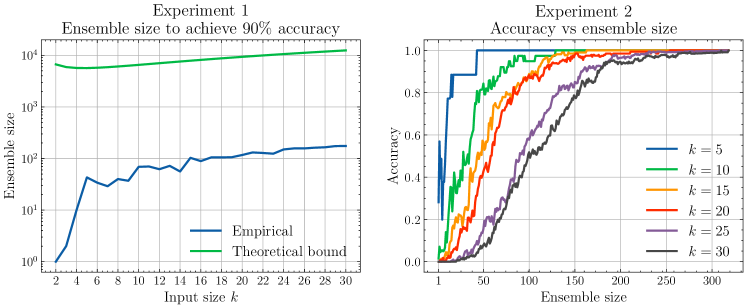
Figure 1: Experiment 1 (left) presents the required number of models (ensemble size) to achieve 90% accuracy as a function of input size $k$, compared to the theoretical bound from Equation 21 with the appropriate $\delta$. Experiment 2 (right) presents accuracy as a function of ensemble size for different input sizes $k$.

In Figure 1, the left plot presents the results of Experiment 1 compared to the bound established in Equation 21 for the appropriate choice of $\delta$ to guarantee $90\%$ accuracy for all test inputs simultaneously. We observe that the empirical ensemble size remains below the theoretical bound, and both curves follow a similar pattern as a function of $k$. For Experiment 2, the results on the right plot of Figure 1 illustrate the convergence to perfect accuracy as a function of the ensemble size for different input sizes $k$. As shown, larger input sizes require more models to achieve perfect accuracy, but with a sufficient number of models, all instances eventually reach perfect accuracy.

8 Conclusion and Future Work

We have demonstrated that, within the NTK framework, an ensemble of simple two-layer fully connected feed-forward neural networks can learn any fixed permutation on binary inputs of size $k$ with arbitrarily high probability from a training set of logarithmic size, namely, the standard basis vectors. Our analysis shows that the network’s output in the infinite width limit converges to a Gaussian process whose mean vector contains precise, sign-based information about the ground truth output. Furthermore, we quantified the number of independent runs required to achieve any desired level of post-rounding accuracy, showing a linearithmic dependence on the input size $k$ for test input, and a quadratic dependence for all input types. In terms of future work we identify a few exciting research directions:

• Generalization Beyond Permutations. Although we focused on learning permutations, it would be interesting to extend our approach to a broader class of functions.

• Wider Range of Architectures. Our analysis centered on a two-layer fully connected feed-forward network. An important direction is exploring whether more sophisticated architectures like multi-layer networks, CNNs, RNNs, or Transformers can exhibit similar exact learning results.

• Exact PAC-Like Framework for NTK Regime. Finally, a crucial next step is to develop a more general PAC-like framework for exact learning guarantees specifically under the NTK regime. This would utilize the infinite-width limit and standard gradient-based training dynamics to give conditions under which neural architectures can learn global transformations with provable exactness.

Appendix

Appendix A Useful Results

In this section, we state and prove some results from linear algebra and probability theory that were used to derive our main results. The following three results were used to derive the required NTK kernels:

Theorem A.1 (Sherman and Morrison 1950).

Suppose $A\in\mathbb{R}^{n\times n}$ is an invertible matrix and $\bm{u},\bm{v}\in\mathbb{R}^{n}$. Then $A+\bm{u}\bm{v}^{\top}$ is invertible if and only if $1+\bm{v}^{\top}A^{-1}\bm{u}\neq 0$. In this case,

$$(A+\bm{u}\bm{v}^{\top})^{-1}=A^{-1}-\frac{A^{-1}\bm{u}\bm{v}^{\top}A^{-1}}{1+\bm{v}^{\top}A^{-1}\bm{u}}$$

Lemma A.1.

Suppose $A\in\mathbb{R}^{n\times n}$, $\bm{a}=[a_{1},\dots,a_{n}]^{\top}\in\mathbb{R}^{n}$ and $\bm{y}\in\mathbb{R}^{n^{2}}$ is given by

$$\bm{y}=\begin{bmatrix}A\bm{e_{1}}\\ A\bm{e_{2}}\\ \vdots\\ A\bm{e_{n}}\end{bmatrix}$$

Then $(\bm{a}^{\top}\otimes I_{n})\bm{y}=A\bm{a}$.

Proof.

Both the right-hand side and left-hand side are vectors of size $n$. We shall show that for each $i=1,2,\dots,n$, the $i$-th entry of the left-hand side is equal to the $i$-th entry of the right-hand side. The $i$-th entry of $A\bm{a}$ is simply given by

$$(A\bm{a})_{i}=\sum_{j=1}^{n}A_{ij}a_{j}$$

Now let $C=\bm{a}^{\top}\otimes I_{n}\in\mathbb{R}^{n\times n^{2}}$. We can easily observe that $C$ has the following block structure:

$$C=\begin{bmatrix}a_{1}I_{n}&a_{2}I_{n}&\dots&a_{n}I_{n}\end{bmatrix}$$

The $i$-th row of $C$ is therefore given by

$$C_{i}=\begin{bmatrix}a_{1}\bm{e_{i}}^{\top}&a_{2}\bm{e_{i}}^{\top}&\dots&a_{n}\bm{e_{i}}^{\top}\end{bmatrix}\in\mathbb{R}^{1\times n^{2}}$$

Thus, the $i$-th entry of the left-hand side is given by

$$C_{i}\bm{y}=\sum_{j=1}^{n}a_{j}\bm{e_{i}}^{\top}A\bm{e_{j}}=\sum_{j=1}^{n}A_{ij}a_{j}=(A\bm{a})_{i}$$

since $\bm{e_{i}}^{\top}A\bm{e_{j}}=A_{ij}$. This concludes the proof.

∎

Lemma A.2.

For variables $(u,v)\sim\mathcal{N}(\bm{0},\Sigma)$ where

$$\Sigma=\begin{bmatrix}\sigma_{u}^{2}&\sigma_{uv}^{2}\\ \sigma_{vu}^{2}&\sigma_{v}^{2}\end{bmatrix}$$

the following two identities hold:

$$\mathbb{E}\left[\mathrm{ReLU}(u)\cdot\mathrm{ReLU}(v)\right]=\frac{\sigma_{u}\sigma_{v}\left(\cos(\theta)\cdot(\pi-\theta)+\sin(\theta)\right)}{2\pi}$$

and

$$\mathbb{E}\left[1_{[u>0]}\cdot 1_{[v>0]}\right]=\frac{\pi-\theta}{2\pi}$$

where

$$\theta=\arccos\left(\frac{\sigma_{uv}^{2}}{\sigma_{u}\cdot\sigma_{v}}\right)$$

and $1_{X}$ denotes the indicator function of the set $X$.

For a proof of Lemma A.2 refer to Section 4.3 of Golikov et al. [2022].

The last result is a concentration bound for sums of Gaussian random variables which we used to derive our ensemble complexity bounds:

Lemma A.3.

Let $X_{1},X_{2},\dots,X_{n}$ be independent Gaussian random variables with mean $\mu$ and variance $\sigma^{2}$ and let $\overline{X}_{n}=\sum_{i=1}^{n}X_{i}$. Then for all $t>0$, we have:

$$\mathbb{P}\left\{|\overline{X}_{n}-\mu|\geq t\right\}\leq 2\exp\left(-\frac{nt^{2}}{2\sigma^{2}}\right)$$

Proof.

We will use the Chernoff technique. Let $\lambda>0$. We have $\overline{X}_{n}-\mu\sim\mathcal{N}\left(0,\frac{\sigma^{2}}{n}\right)$ and so by symmetry and Markov’s inequality we get:

$$\mathbb{P}\left\{|\overline{X}_{n}-\mu|\geq t\right\} =2\mathbb{P}\left\{\overline{X}_{n}-\mu\geq t\right\}=2\mathbb{P}\left\{e^{\lambda(\overline{X}_{n}-\mu)}\geq e^{\lambda t}\right\}\leq e^{-\lambda t}\cdot\mathbb{E}\left[e^{\lambda(\overline{X}_{n}-\mu)}\right]$$ (22)

The expectation on the right-hand side is equal to the moment-generating function of a normal distribution with mean $0$ and variance $\sigma^{2}/n$ and so it is equal to $\exp\left(\frac{\sigma^{2}\lambda^{2}}{2n}\right)$. Now let

$$\phi(\lambda)=\exp\left(\frac{\sigma^{2}\lambda^{2}}{2n}-\lambda t\right)$$

be the right-hand side of Equation 22. Minimizing $\phi(\lambda)$ with respect to $\lambda$ we find that the minimum occurs at $\lambda^{*}=\frac{nt}{\sigma^{2}}$ and plugging this back into Equation 22 gives the required bound. ∎

Appendix B Recursive formulas for the NTK and NNGP Kernels

In this section, we provide the recursive formulas used to derive the NNGP and limit NTK kernels defined in Section 3. In the following, the notation is consistent with that of Section 3.

The NNGP Kernel

As the width of the network tends to infinity, it has been shown that the network at initialization behaves as a Gaussian process. That is, the stacked pre-activation outputs at each layer $l$ at initialization, $f_{0}^{l}(\mathcal{X})$ converges to a multivariate Gaussian distribution $\mathcal{N}(\bm{0},\mathcal{K}^{l}(\mathcal{X},\mathcal{X}))$ where the covariance matrix $\mathcal{K}$ can be computed using the formula

$$\mathcal{K}^{l}(\bm{x},\bm{x^{\prime}})=\tilde{\mathcal{K}}^{l}(\bm{x},\bm{x^{\prime}})I_{n_{l}}$$

where

$$\tilde{\mathcal{K}}^{l}\left(\bm{x},\bm{x}^{\prime}\right)=\sigma_{\omega}^{2}\mathcal{T}\left(\left[\begin{array}[]{ll}\tilde{\mathcal{K}}^{l-1}(\bm{x},\bm{x})&\tilde{\mathcal{K}}^{l-1}\left(\bm{x},\bm{x}^{\prime}\right)\\ \tilde{\mathcal{K}}^{l-1}\left(\bm{x},\bm{x}^{\prime}\right)&\tilde{\mathcal{K}}^{l-1}\left(\bm{x}^{\prime},\bm{x}^{\prime}\right)\end{array}\right]\right)+\sigma_{b}^{2}$$ (23)

with base case $\tilde{\mathcal{K}}^{1}(\bm{x},\bm{x^{\prime}})=\sigma_{\omega}^{2}\cdot\frac{1}{n_{0}}\bm{x}^{\top}\bm{x^{\prime}}+\sigma_{b}^{2}$. The function $\mathcal{T}$ maps a $2\times 2$ positive semi-definite matrix $\Sigma$ to $\mathbb{E}[\phi(u)\phi(v)]$ for $(u,v)\sim\mathcal{N}(\bm{0},\Sigma)$. For details see Lee et al. [2018] and Appendix E. of Lee et al. [2019].

Limit NTK

It can be shown that in the infinite width limit, the empirical NTK at initialization $\hat{\Theta}^{l}_{0}$ converges to a deterministic kernel $\Theta^{l}$ given by the formula

$$\Theta^{l}(\bm{x},\bm{x^{\prime}})=\tilde{\Theta}^{l}(\bm{x},\bm{x^{\prime}})I_{n_{l}}$$

where

$$\tilde{\Theta}^{l} \left(\bm{x},\bm{x}^{\prime}\right)=\tilde{\mathcal{K}}^{l}\left(\bm{x},\bm{x}^{\prime}\right)+\sigma_{\omega}^{2}\tilde{\Theta}^{l-1}\left(\bm{x},\bm{x}^{\prime}\right)\dot{\mathcal{T}}\left(\left[\begin{array}[]{cc}\tilde{\mathcal{K}}^{l-1}(\bm{x},\bm{x})&\tilde{\mathcal{K}}^{l-1}\left(\bm{x},\bm{x}^{\prime}\right)\\ \tilde{\mathcal{K}}^{l-1}\left(\bm{x},\bm{x}^{\prime}\right)&\tilde{\mathcal{K}}^{l-1}\left(\bm{x}^{\prime},\bm{x}^{\prime}\right)\end{array}\right]\right)$$ (26)

with base case $\tilde{\Theta}^{1}(\bm{x},\bm{x^{\prime}})=\tilde{\mathcal{K}}^{1}(\bm{x},\bm{x^{\prime}})$, and $\tilde{\mathcal{K}}^{l}$ is as defined in the previous paragraph. The function $\dot{\mathcal{T}}$ maps a $2\times 2$ positive semi-definite matrix $\Sigma$ to $\mathbb{E}[\phi^{\prime}(u)\phi^{\prime}(v)]$ for $(u,v)\sim\mathcal{N}(\bm{0},\Sigma)$. For more details refer to Jacot et al. [2018] and Appendix E. of Lee et al. [2019]

Remark B.1.

In the case of ReLU activation, Lemma A.2 gives closed-form expressions for both $\mathcal{T}$ and $\mathcal{\dot{T}}$.

Appendix C Derivations of Train and Test NTK Matrices

This section serves as a supplement to Section 5 of the main paper. Here, we provide an outline of how the formulas for the train and test NTK matrices on the main paper can be derived using the results of Appendix B. For clarity, we separate the derivation of train and test NTK matrices into two subsections.

C.1 Train NTK

Since the training set consists of the standard basis vectors, to get the train NTK kernel we need to compute $\mathcal{K}^{l}(\bm{e_{i}},\bm{e_{j}})$ and $\Theta^{l}(\bm{e_{i}},\bm{e_{j}})$ for $l=1,2$ and $i,j\in[k]$. We will use the results of Appendix B to compute them. We can easily see that the base case gives

$$\tilde{\mathcal{K}}^{1}(\bm{e_{i}},\bm{e_{j}})=\begin{cases}\frac{\sigma_{\omega}^{2}}{k}+\sigma_{b}^{2}&\text{if }i=j\\ \sigma_{b}^{2}&\text{if }i\neq j\end{cases}$$ (27)

Using the recursive formula of Equation 23 we get for $i\neq j$

$$\tilde{\mathcal{K}}^{2}\left(\bm{e_{i}},\bm{e_{j}}\right) =\sigma_{\omega}^{2}\mathcal{T}\left(\begin{bmatrix}\frac{\sigma_{\omega}^{2}}{k}+\sigma_{b}^{2}&\sigma_{b}^{2}\\ \sigma_{b}^{2}&\frac{\sigma_{\omega}^{2}}{k}+\sigma_{b}^{2}\end{bmatrix}\right)+\sigma_{b}^{2}$$

$$=\sigma_{\omega}^{2}\left(\frac{\sigma_{\omega}^{2}}{k}+\sigma_{b}^{2}\right)\cdot\frac{\cos\theta\cdot(\pi-\theta)+\sin\theta}{2\pi}+\sigma_{b}^{2}$$ (28)

where

$$\theta=\arccos\left(\frac{\sigma_{b}^{2}}{\frac{\sigma_{\omega}^{2}}{k}+\sigma_{b}^{2}}\right)$$ (29)

Similarly, for $i=j$ we have

$$\tilde{\mathcal{K}}^{2}\left(\bm{e_{i}},\bm{e_{j}}\right) =\sigma_{\omega}^{2}\mathcal{T}\left(\begin{bmatrix}\frac{\sigma_{\omega}^{2}}{k}+\sigma_{b}^{2}&\frac{\sigma_{\omega}^{2}}{k}+\sigma_{b}^{2}\\ \frac{\sigma_{\omega}^{2}}{k}+\sigma_{b}^{2}&\frac{\sigma_{\omega}^{2}}{k}+\sigma_{b}^{2}\end{bmatrix}\right)+\sigma_{b}^{2}$$

$$=\frac{\sigma_{\omega}^{2}}{2}\left(\frac{\sigma_{\omega}^{2}}{k}+\sigma_{b}^{2}\right)+\sigma_{b}^{2}$$ (30)

Hence, substituting $\sigma_{\omega}=1$ and $\sigma_{b}=0$ above we get

$$\mathcal{K}(\mathcal{X},\mathcal{X})=\left(\left(\frac{d}{2}-c\right)I_{k}+c\bm{1}\bm{1}^{\top}\right)\otimes I_{k}\in\mathbb{R}^{k^{2}\times k^{2}}$$ (31)

where $d$ and $c$ are as in Equation 4. In both cases, we used Lemma A.2 to compute the function $\mathcal{T}$. In a similar fashion, following the recursive formula of Equation 26 and using Lemma A.2 we arrive at the limit NTK kernel of Equation 3.

C.2 Test NTK

To obtain an expression of the test NTK we again need to calculate $\mathcal{K}^{l}(\hat{\bm{x}},\bm{e_{i}})$ and $\Theta^{l}(\hat{\bm{x}},\bm{e_{i}})$ for any $\hat{\bm{x}}\in\mathbb{K}$, $l=1,2$ and $i\in[k]$. Consider an arbitrary test input $\hat{\bm{x}}\in\mathbb{K}$ and a basis vector $\bm{e_{i}}$. From the base case of the recursion we have

$$\tilde{\mathcal{K}}^{1}(\bm{\hat{x}},\bm{e_{i}})=\begin{cases}\frac{\sigma_{\omega}^{2}\hat{\bm{x}}_{i}}{k}+\sigma_{b}^{2}&\text{if }\hat{\bm{x}}_{i}>0\\ \sigma_{b}^{2}&\text{if }\hat{\bm{x}}_{i}=0\end{cases}$$ (32)

and (since $\hat{\bm{x}}$ is normalized)

$$\tilde{\mathcal{K}}^{1}(\hat{\bm{x}},\hat{\bm{x}})=\frac{\sigma_{\omega}^{2}}{k}+\sigma_{b}^{2}$$ (33)

where $n_{\hat{\bm{x}}}$ denotes the number of nonzero entries of $\hat{\bm{x}}$. Using Equation 23 we get

$$\tilde{\mathcal{K}}^{2}(\hat{\bm{x}},\bm{e_{i}}) =\sigma_{\omega}^{2}\mathcal{T}\left(\begin{bmatrix}\frac{\sigma_{\omega}^{2}}{k}+\sigma_{b}^{2}&\frac{\sigma_{\omega}^{2}\hat{\bm{x}}_{i}}{k}+\sigma_{b}^{2}\\ \frac{\sigma_{\omega}^{2}\hat{\bm{x}}_{i}}{k}+\sigma_{b}^{2}&\frac{\sigma_{\omega}^{2}}{k}+\sigma_{b}^{2}\end{bmatrix}\right)+\sigma_{b}^{2}$$

$$=\sigma_{\omega}^{2}\left(\frac{\sigma_{\omega}^{2}}{k}+\sigma_{b}^{2}\right)\cdot\frac{\cos\hat{\theta}_{i}(\pi-\hat{\theta}_{i})+\sin\hat{\theta}_{i}}{2\pi}+\sigma_{b}^{2}$$ (34)

where

$$\hat{\theta_{i}}=\arccos\left(\frac{\sigma_{\omega}^{2}\frac{\hat{\bm{x}}_{i}}{k}+\sigma_{b}^{2}}{\frac{\sigma_{\omega}^{2}}{k}+\sigma_{b}^{2}}\right)$$ (35)

The second equality follows from Lemma A.2. Substituting $\sigma_{\omega}=1$ and $\sigma_{b}=0$ we therefore have

$$\mathcal{K}(\hat{\bm{x}},\mathcal{X})=\mathbf{g}^{\top}\otimes I_{k}\in\mathbb{R}^{k\times k^{2}}$$ (36)

with $\mathbf{g}\in\mathbb{R}^{k}$ as in Equation 18. Similarly, we obtain the expression for the test NTK of Equation 6.

Appendix D Proof of Lemma 6.1

In this section, we analyze the mean and variance of the predictions under the limit NTK, expressing them as functions of the test vector $\hat{\bm{x}}$. Specifically, we characterize their dependence on the vector length $k$ and the number of nonzero elements $n_{\hat{\bm{x}}}$. We establish that the variance of the predictions scales as $\mathcal{O}\left(1/k\right)$ while the mean coordinates exhibit two different behaviors: they scale with $\Theta(\nicefrac{{\sqrt{n_{\hat{\bm{x}}}}}}{{k}})$ when $P^{*}\hat{\bm{x}}=0$ and $\Theta(\nicefrac{{1}}{{k}})$ when $P^{*}\hat{\bm{x}}>0$.

Preliminary quantities

We begin by rewriting several useful expressions from Section 5 and adding other relevant expressions to complement them. For $\sigma_{w}=1$ and $\sigma_{b}=0$ as defined in Section 4, recall:

$$d=\frac{1}{k}\quad\textrm{ and }\quad c=\frac{1}{2\pi k}$$

We further introduce

$$d^{\prime}=\frac{d}{2}=\frac{1}{2k}\quad\textrm{ and }\quad c^{\prime}=c=\frac{1}{2\pi k}$$

Additionally, we rewrite Equation 9 in an alternative form:

$$\hat{\theta}_{i}=\begin{cases}\arccos\left(\frac{1}{\sqrt{n_{\hat{\bm{x}}}}}\right)&\textrm{if }\hat{\bm{x}}_{i}\neq 0\\ \frac{\pi}{2}&\textrm{otherwise}\end{cases}$$

From this, we directly obtain the cosine and sine of $\hat{\theta}_{i}$:

$$\cos\hat{\theta}_{i}=\begin{cases}\frac{1}{\sqrt{n_{\hat{\bm{x}}}}}&\textrm{if }\hat{\bm{x}}_{i}\neq 0\\ 0&\textrm{otherwise}\end{cases}\qquad\sin\hat{\theta}_{i}=\begin{cases}\sqrt{1-\frac{1}{n_{\hat{\bm{x}}}}}&\textrm{if }\hat{\bm{x}}_{i}\neq 0\\ 1&\textrm{otherwise}\end{cases}$$

Using these quantities, we rewrite Equation 18 as:

$$\mathbf{g}_{i}=\begin{cases}\frac{1}{2\pi k\sqrt{n_{\hat{\bm{x}}}}}\left(\pi-\arccos\left(\nicefrac{{1}}{{\sqrt{n_{\hat{\bm{x}}}}}}\right)+\sqrt{n_{\hat{\bm{x}}}-1}\right)&\textrm{if }\hat{\bm{x}}_{i}\neq 0\\ \frac{1}{2\pi k}&\textrm{otherwise}\end{cases}$$

and Equation 7 as

$$\mathbf{f}_{i}=\begin{cases}\mathbf{g}_{i}+\frac{\pi-\arccos\left(\nicefrac{{1}}{{\sqrt{n_{\hat{\bm{x}}}}}}\right)}{2\pi k\sqrt{n_{\hat{\bm{x}}}}}&\textrm{if }\hat{\bm{x}}_{i}\neq 0,\\ \mathbf{g}_{i}&\textrm{otherwise}\end{cases}$$

D.1 Computing the mean $\mu(\hat{\bm{x}})$

We first recall the expression for the mean:

$$\mu(\hat{\bm{x}})=P^{*}\left(\frac{1}{d-c}I_{k}-\frac{c}{(d-c)(d-c+ck)}\bm{1}\bm{1}^{\top}\right)\mathbf{f}$$

which we decompose into two terms:

$$\mu(\hat{\bm{x}})=\frac{P^{*}\mathbf{f}}{d-c}-\frac{c\bm{1}\bm{1}^{\top}\mathbf{f}}{(d-c)(d-c+ck)}$$ (37)

The second term simplifies since $\bm{1}$ is the vector of all ones, effectively absorbing the permutation $P^{*}$. For the first term in Equation 37, we obtain:

$$\frac{(P_{j}^{*})^{\top}\mathbf{f}}{d-c}=\begin{cases}\frac{1}{2\pi-1}\left(\frac{\pi-\arccos\left(\nicefrac{{1}}{{\sqrt{n_{\hat{\bm{x}}}}}}\right)}{\sqrt{n_{\hat{\bm{x}}}}}+\sqrt{1-\frac{1}{\sqrt{n_{\hat{\bm{x}}}}}}\right)&\textrm{if }\hat{\bm{x}}_{j}\neq 0\\ \frac{1}{2\pi-1}&\textrm{otherwise}\end{cases}$$

The second term is a constant vector with coefficient:

$$\frac{c\bm{1}\bm{1}^{\top}\mathbf{f}}{(d-c)(d-c+ck)}=\frac{1}{(2\pi-1)(2\pi-1+k)}\left(\frac{n_{\hat{\bm{x}}}\left(\pi-\arccos\left(\nicefrac{{1}}{{\sqrt{n_{\hat{\bm{x}}}}}}\right)\right)}{2\sqrt{n_{\hat{\bm{x}}}}}+n_{\hat{\bm{x}}}\sqrt{1-\frac{1}{n_{\hat{\bm{x}}}}}+k-n_{\hat{\bm{x}}}\right)$$

We now evaluate each case of the mean separately.

Case 1: For $\mu_{0}(\hat{\bm{x}})$, that is, when $P^{*}\hat{\bm{x}}=0$, we have:

$$\mu_{0}(\hat{\bm{x}})= \frac{1}{2\pi-1}\left(1-\frac{k-n_{\hat{\bm{x}}}}{2\pi+k-1}-\frac{2\pi kn_{\hat{x}}}{\left(2\pi+k-1\right)\left(\pi k\sqrt{n_{\hat{\bm{x}}}}\right)}\left(\pi-\arccos\left(\nicefrac{{1}}{{\sqrt{n_{\hat{\bm{x}}}}}}\right)\right)\right)$$

$$- \frac{1}{2\pi-1}\left(\frac{2\pi kn_{\hat{x}}}{\left(2\pi+k-1\right)\left(2\pi k\right)}\sqrt{1-\frac{1}{\sqrt{n_{\hat{\bm{x}}}}}}\right)$$ (38)

This expression behaves like $\Theta\left(\sqrt{n_{\hat{\bm{x}}}}/k\right)$, and setting $n_{\hat{\bm{x}}}$ to different regimes yields the bounds established in Lemma 6.1, namely:

$$\mu_{0}(\hat{\bm{x}})\in\begin{cases}\Theta\left(1/k\right)&\text{if}\;n_{\hat{\bm{x}}}\text{ is constant}\\ \Theta\left(\sqrt{n_{\hat{\bm{x}}}}/k\right)&\text{if}\;n_{\hat{\bm{x}}}\text{ is non-constant}\\ &\text{and sublinear in }k\\ \Theta\left(1/\sqrt{k}\right)&\text{if}\;n_{\hat{\bm{x}}}=ck\text{ for }c\in(0,1]\end{cases}$$

Case 2: For $\mu_{1}(\hat{\bm{x}})$, that is, when $P^{*}\hat{\bm{x}}>0$, we have:

$$\mu_{1}(\hat{\bm{x}})= \frac{2\pi-1}{2\pi+k-1}\left(\frac{2}{\left(2\pi-1\right)\sqrt{n_{\hat{\bm{x}}}}}\left(\pi-\arccos\left(\nicefrac{{1}}{{\sqrt{n_{\hat{\bm{x}}}}}}\right)\right)+\frac{1}{\left(2\pi-1\right)}\sqrt{1-\frac{1}{\sqrt{n_{\hat{\bm{x}}}}}}\right)$$

$$+\frac{k-n_{\hat{\bm{x}}}}{2\pi+k-1}\left(\frac{2}{\left(2\pi-1\right)\sqrt{n_{\hat{\bm{x}}}}}\left(\pi-\arccos\left(\nicefrac{{1}}{{\sqrt{n_{\hat{\bm{x}}}}}}\right)\right)+\frac{1}{\left(2\pi-1\right)}\sqrt{1-\frac{1}{\sqrt{n_{\hat{\bm{x}}}}}}-\frac{1}{\left(2\pi-1\right)}\right)$$ (39)

When setting $n_{\hat{\bm{x}}}=k$, we note that the second term becomes zero and the first term becomes $\Theta\left(1/k\right)$. Alternatively, the first term in Section D.1 is $\Theta\left(1/k\right)$ and the second term is $\Theta\left(1/\sqrt{n_{\hat{\bm{x}}}}\right)$, implying $\mu(\hat{\bm{x}})_{1}\in\Theta\left(1/\sqrt{n_{\hat{\bm{x}}}}\right)$. Setting $n_{\hat{\bm{x}}}$ to different regimes yields the bounds established in Lemma 6.1, namely:

$$\mu_{1}(\hat{\bm{x}})\in\begin{cases}\Theta\left(1/\sqrt{n_{\hat{\bm{x}}}}\right)&\text{if}\;n_{\hat{\bm{x}}}\text{ is non-constant}\\ &\text{and sublinear in }k,\\ \Theta\left(1/\sqrt{k}\right)&\text{if}\;n_{\hat{\bm{x}}}=ck\text{ for }c\in(0,1)\\ \Theta\left(1/k\right)&\text{if}\;n_{\hat{\bm{x}}}=k\end{cases}$$

D.2 Computing the variance $\Sigma(\hat{\bm{x}})$

We begin by recalling the expression for the variance (substituting $d^{\prime}$ and $c^{\prime}$):

$$\Sigma(\hat{\bm{x}})=\left(d^{\prime}+\mathbf{f}^{\top}AMA\mathbf{f}-2\mathbf{f}^{\top}A\mathbf{g}\right)I_{k}$$

where

$$M=\left(d^{\prime}-c^{\prime}\right)I_{k}+c^{\prime}\bm{1}\bm{1}^{\top}\quad\textrm{ and }\quad A=\frac{1}{d-c}I_{k}-\frac{c}{(d-c)(d-c+ck)}\bm{1}\bm{1}^{\top}$$

We aim to show that the variance is bounded by $\mathcal{O}\left(1/k\right)$. To facilitate this, we rewrite $\Sigma(\hat{\bm{x}})$ by expanding the matrix multiplication:

$$\Sigma(\hat{\bm{x}}) =d^{\prime}I_{k}+\mathbf{f}^{\top}\left(AMA\mathbf{f}-2A(\mathbf{f}-\mathbf{z})\right)I_{k}$$

$$=d^{\prime}I_{k}+\mathbf{f}^{\top}\left(AMA\mathbf{f}-2A\mathbf{f}\right)I_{k}+2\mathbf{f}^{\top}A\mathbf{z}I_{k}$$

where we define $\mathbf{z}=\mathbf{f}-\mathbf{g}$ for notational simplicity. It is straightforward to observe that the first term, $d^{\prime}I_{k}$, is bounded by $\mathcal{O}\left(1/k\right)$. Thus, we focus our attention on the remaining two terms. For the second term, we begin by showing that $AMA-2A$ has a maximum eigenvalue of $\mathcal{O}(1)$, and therefore:

$$\mathbf{f}^{\top}(AMA-2A)\mathbf{f}\in\mathcal{O}\left(1/k\right)$$

We begin by expressing $AMA$ in a more manageable form. A direct computation reveals:

$$AMA=uI_{k}-v\bm{1}\bm{1}^{\top}$$

where

$$u=\frac{d^{\prime}-c^{\prime}}{\left(d-c\right)^{2}}\quad\textrm{ and }\quad v=\frac{1}{k}\left(\frac{d^{\prime}-c^{\prime}+kc^{\prime}}{\left(d-c+kc\right)^{2}}-\frac{d^{\prime}-c^{\prime}}{\left(d-c\right)^{2}}\right)$$

Subtracting $2A$ from this expression gives:

$$AMA-2A=\left(u-2a\right)I_{k}+\left(v+2b\right)\bm{1}\bm{1}^{\top}$$

where

$$a=\frac{d-c}{\left(d-c\right)^{2}}\quad\textrm{ and }\quad b=\frac{c}{\left(d-c+ck\right)\left(d-c\right)}$$

This matrix has two unique eigenvalues: $u-2a$ (with multiplicity $k-1$) and $u-2a+(v+2b)k$. We will show that the largest eigenvalue is $\mathcal{O}(1)$. To this end, we evaluate these two quantities, starting with $u-2a$:

$$u-2a =\frac{d^{\prime}-c^{\prime}-2(d-c)}{(d-c)^{2}}$$

$$=-\frac{2\pi(3\pi-1)k}{(2\pi-1)^{2}}$$

which is negative. For the second eigenvalue, we find:

$$u-2a+(v+2b)k =-\frac{2\pi(3\pi-1)k}{(2\pi-1)^{2}}+\frac{2\pi k\left(\pi+k-1\right)}{\left(2\pi+k-1\right)^{2}}-\frac{2\pi k(\pi-1)}{\left(2\pi-1\right)^{2}}+\frac{4\pi k}{\left(2\pi-1\right)\left(2\pi+k-1\right)}$$

$$=\left(\frac{4\pi}{2\pi+k-1}+\frac{\pi+k-1}{(2\pi+k-1)^{2}}\right)k$$

which is positive and clearly $\mathcal{O}(1)$. With this result, we can bound the multiplication by the norms of its components. Since $\lambda_{\max}(AMA-2A)\in\mathcal{O}(1)$ and $\|\mathbf{f}\|^{2}\in\mathcal{O}\left(1/k\right)$ (since each $\mathbf{f}_{i}\in\mathcal{O}\left(1/k\right))$, we conclude:

$$\mathbf{f}^{\top}(AMA-2A)\mathbf{f}\in\mathcal{O}\left(1/k\right)$$

We now turn to the third term, $2\mathbf{f}^{\top}A\mathbf{z}$. Expressing $\mathbf{z}$ component-wise we have:

$$\mathbf{z}_{i}=\begin{cases}\frac{\pi-\arccos\left(\nicefrac{{1}}{{\sqrt{n_{\hat{\bm{x}}}}}}\right)}{2\pi k\sqrt{n_{\hat{\bm{x}}}}}&\textrm{if }\hat{\bm{x}}_{i}\neq 0\\ 0&\textrm{otherwise}\end{cases}$$

We then decompose the product $\mathbf{f}^{\top}A\mathbf{z}$ as:

$$\mathbf{f}^{\top}A\mathbf{z}=a\mathbf{f}^{\top}\mathbf{z}-b(\mathbf{f}^{\top}\mathbf{1})(\mathbf{1}^{\top}\mathbf{z})$$ (40)

where

$$a=\frac{1}{d-c}\quad\textrm{ and }\quad b=\frac{2\pi k}{(2\pi-1)(2\pi+k-1)}$$

The first term $a\mathbf{f}^{\top}\mathbf{z}$ can be expressed as:

$$a\mathbf{f}^{\top}\mathbf{z}=\frac{1}{(2\pi-1)(2\pi k)^{2}}\left(2\pi-2\arccos\left(\nicefrac{{1}}{{\sqrt{n_{\hat{\bm{x}}}}}}\right)-\sqrt{n_{\hat{\bm{x}}}-1}\right)\left(\pi-2\arccos\left(\nicefrac{{1}}{{\sqrt{n_{\hat{\bm{x}}}}}}\right)\right)$$

which is positive and $\mathcal{O}\left(1/k\right)$. For the second term $b(\mathbf{f}^{\top}\bm{1})(\bm{1}^{\top}\mathbf{z})$, we start by expressing the individual quantities $\mathbf{f}^{\top}\mathbf{1}$ and $\mathbf{1}^{\top}\mathbf{z}$:

$$\mathbf{f}^{\top}\mathbf{1}=\frac{\sqrt{n_{\hat{\bm{x}}}}}{\pi k}\left(\pi-\arccos\left(\nicefrac{{1}}{{\sqrt{n_{\hat{\bm{x}}}}}}\right)\right)+\frac{\sqrt{n_{\hat{\bm{x}}}}\sqrt{n_{\hat{\bm{x}}}-1}}{2\pi k}+\frac{k-n_{\hat{\bm{x}}}}{2\pi k}$$

and

$$\mathbf{1}^{\top}\mathbf{z}=\frac{\sqrt{n_{\hat{\bm{x}}}}}{2\pi k}\left(\pi-\arccos\left(\nicefrac{{1}}{{\sqrt{n_{\hat{\bm{x}}}}}}\right)\right)$$

Therefore, the entire term can be expressed as:

$$b(\mathbf{f}^{\top}\bm{1})(\bm{1}^{\top}\mathbf{z})=\frac{1}{2\pi k(2\pi-1)(2\pi-1+k)}\Big{(} 2n\left(\pi-\arccos\left(\nicefrac{{1}}{{\sqrt{n_{\hat{\bm{x}}}}}}\right)\right)^{2}$$

$$+n\sqrt{n-1}\left(\pi-\arccos\left(\nicefrac{{1}}{{\sqrt{n_{\hat{\bm{x}}}}}}\right)\right)$$

$$+(k-n)\sqrt{n_{\hat{\bm{x}}}}\left(\pi-\arccos\left(\nicefrac{{1}}{{\sqrt{n_{\hat{\bm{x}}}}}}\right)\right)\Big{)}$$

which is positive and $\mathcal{O}\left(1/k\right)$, therefore, the subtraction of Equation 40 (which is equal to $\mathbf{f}^{\top}A\mathbf{z}$) is $\mathcal{O}\left(1/k\right)$. Combining the bounds on all three terms, we conclude that:

$$\Sigma(\hat{\bm{x}})\in\mathcal{O}\left(1/k\right)I_{k}$$

completing the proof of the second part of Lemma 6.1.

References

- Adlam and Pennington (2020) Ben Adlam and Jeffrey Pennington. The neural tangent kernel in high dimensions: Triple descent and a multi-scale theory of generalization. In Hal Daumé III and Aarti Singh, editors, Proceedings of the 37th International Conference on Machine Learning, volume 119 of Proceedings of Machine Learning Research, pages 74–84. PMLR, 13–18 Jul 2020. URL https://proceedings.mlr.press/v119/adlam20a.html.
- Back De Luca and Fountoulakis (2024) Artur Back De Luca and Kimon Fountoulakis. Simulation of graph algorithms with looped transformers. In Proceedings of the 41st International Conference on Machine Learning, volume 235 of Proceedings of Machine Learning Research, pages 2319–2363. PMLR, 2024. URL https://dl.acm.org/doi/10.5555/3692070.3692162.
- Back de Luca et al. (2025) Artur Back de Luca, George Giapitzakis, Shenghao Yang, Petar Veličković, and Kimon Fountoulakis. Positional attention: Expressivity and learnability of algorithmic computation, 2025. URL https://arxiv.org/abs/2410.01686.
- Ben-David et al. (2006) Shai Ben-David, John Blitzer, Koby Crammer, and Fernando Pereira. Analysis of representations for domain adaptation. In B. Schölkopf, J. Platt, and T. Hoffman, editors, Advances in Neural Information Processing Systems, volume 19. MIT Press, 2006. URL https://proceedings.neurips.cc/paper_files/paper/2006/file/b1b0432ceafb0ce714426e9114852ac7-Paper.pdf.
- Boix-Adserà et al. (2024) Enric Boix-Adserà, Omid Saremi, Emmanuel Abbe, Samy Bengio, Etai Littwin, and Joshua M. Susskind. When can transformers reason with abstract symbols? In The Twelfth International Conference on Learning Representations, 2024. URL https://openreview.net/forum?id=STUGfUz8ob.
- Cybenko (1989) G. Cybenko. Approximation by superpositions of a sigmoidal function. Mathematics of Control, Signals and Systems, 2(4):303–314, 1989. doi: 10.1007/BF02551274. URL https://doi.org/10.1007/BF02551274.
- Giannou et al. (2023) Angeliki Giannou, Shashank Rajput, Jy-Yong Sohn, Kangwook Lee, Jason D. Lee, and Dimitris Papailiopoulos. Looped transformers as programmable computers. In Proceedings of the 40th International Conference on Machine Learning, volume 202, pages 11398–11442, 2023. URL https://dl.acm.org/doi/10.5555/3618408.3618866.
- Golikov et al. (2022) Eugene Golikov, Eduard Pokonechnyy, and Vladimir Korviakov. Neural tangent kernel: A survey, 2022. URL https://arxiv.org/abs/2208.13614.
- Hertrich and Skutella (2023) Christoph Hertrich and Martin Skutella. Provably good solutions to the knapsack problem via neural networks of bounded size. INFORMS journal on computing, 35(5):1079–1097, 2023. URL https://pubsonline.informs.org/doi/10.1287/ijoc.2021.0225.
- Hornik et al. (1989) Kurt Hornik, Maxwell Stinchcombe, and Halbert White. Multilayer feedforward networks are universal approximators. Neural Networks, 2(5):359–366, 1989. ISSN 0893-6080. doi: https://doi.org/10.1016/0893-6080(89)90020-8. URL https://www.sciencedirect.com/science/article/pii/0893608089900208.
- (11) Wolfram Research, Inc. Mathematica, Version 14.1. URL https://www.wolfram.com/mathematica. Champaign, IL, 2024.
- Jacot et al. (2018) Arthur Jacot, Franck Gabriel, and Clement Hongler. Neural tangent kernel: Convergence and generalization in neural networks. In S. Bengio, H. Wallach, H. Larochelle, K. Grauman, N. Cesa-Bianchi, and R. Garnett, editors, Advances in Neural Information Processing Systems, volume 31. Curran Associates, Inc., 2018. URL https://proceedings.neurips.cc/paper_files/paper/2018/file/5a4be1fa34e62bb8a6ec6b91d2462f5a-Paper.pdf.
- Lee et al. (2018) Jaehoon Lee, Jascha Sohl-dickstein, Jeffrey Pennington, Roman Novak, Sam Schoenholz, and Yasaman Bahri. Deep neural networks as gaussian processes. In International Conference on Learning Representations, 2018. URL https://openreview.net/forum?id=B1EA-M-0Z.
- Lee et al. (2019) Jaehoon Lee, Lechao Xiao, Samuel Schoenholz, Yasaman Bahri, Roman Novak, Jascha Sohl-Dickstein, and Jeffrey Pennington. Wide neural networks of any depth evolve as linear models under gradient descent. In H. Wallach, H. Larochelle, A. Beygelzimer, F. d'Alché-Buc, E. Fox, and R. Garnett, editors, Advances in Neural Information Processing Systems, volume 32. Curran Associates, Inc., 2019. URL https://proceedings.neurips.cc/paper_files/paper/2019/file/0d1a9651497a38d8b1c3871c84528bd4-Paper.pdf.
- Mansour et al. (2009) Yishay Mansour, Mehryar Mohri, and Afshin Rostamizadeh. Domain adaptation: Learning bounds and algorithms. In Proceedings of The 22nd Annual Conference on Learning Theory (COLT 2009), Montréal, Canada, 2009. URL http://www.cs.nyu.edu/~mohri/postscript/nadap.pdf.
- Nakkiran et al. (2020) Preetum Nakkiran, Gal Kaplun, Yamini Bansal, Tristan Yang, Boaz Barak, and Ilya Sutskever. Deep double descent: Where bigger models and more data hurt. In International Conference on Learning Representations, 2020. URL https://openreview.net/forum?id=B1g5sA4twr.
- Pérez et al. (2021) Jorge Pérez, Pablo Barceló, and Javier Marinkovic. Attention is turing-complete. Journal of Machine Learning Research, 22(75):1–35, 2021. URL https://dl.acm.org/doi/pdf/10.5555/3546258.3546333.
- Sherman and Morrison (1950) Jack Sherman and Winifred J. Morrison. Adjustment of an inverse matrix corresponding to a change in one element of a given matrix. The Annals of Mathematical Statistics, 21(1):124–127, 1950. ISSN 00034851. URL http://www.jstor.org/stable/2236561.
- Siegelmann and Sontag (1995) Hava Siegelmann and Eduardo Sontag. On the computational power of neural nets. Journal of Computer and System Sciences, 50:132–150, 1995. URL https://www.sciencedirect.com/science/article/pii/S0022000085710136.
- Singh et al. (2022) Sidak Pal Singh, Aurelien Lucchi, Thomas Hofmann, and Bernhard Schölkopf. Phenomenology of double descent in finite-width neural networks. In International Conference on Learning Representations, 2022. URL https://openreview.net/forum?id=lTqGXfn9Tv.
- Wang et al. (2022) Sifan Wang, Xinling Yu, and Paris Perdikaris. When and why pinns fail to train: A neural tangent kernel perspective. Journal of Computational Physics, 449:110768, 2022. ISSN 0021-9991. doi: https://doi.org/10.1016/j.jcp.2021.110768. URL https://www.sciencedirect.com/science/article/pii/S002199912100663X.
- Wei et al. (2022) Colin Wei, Yining Chen, and Tengyu Ma. Statistically meaningful approximation: a case study on approximating turing machines with transformers. Advances in Neural Information Processing Systems, 35:12071–12083, 2022. URL https://dl.acm.org/doi/10.5555/3600270.3601147.
- Yang (2020) Greg Yang. Tensor programs ii: Neural tangent kernel for any architecture, 2020. URL https://arxiv.org/abs/2006.14548.
- Yang and Littwin (2021) Greg Yang and Etai Littwin. Tensor programs iib: Architectural universality of neural tangent kernel training dynamics, 2021. URL https://arxiv.org/abs/2105.03703.
- Yang et al. (2024) Liu Yang, Kangwook Lee, Robert D Nowak, and Dimitris Papailiopoulos. Looped transformers are better at learning learning algorithms. In The Twelfth International Conference on Learning Representations, 2024. URL https://openreview.net/forum?id=HHbRxoDTxE.
- Yuqing et al. (2022) Li Yuqing, Luo Tao, and Kwan Yip, Nung. Towards an understanding of residual networks using neural tangent hierarchy (nth). CSIAM Transactions on Applied Mathematics, 3(4):692–760, 2022. ISSN 2708-0579. doi: https://doi.org/10.4208/csiam-am.SO-2021-0053. URL https://global-sci.com/article/82332/towards-an-understanding-of-residual-networks-using-neural-tangent-hierarchy-nth.