Towards Optimal Adversarial Robust Reinforcement Learning with Infinity Measurement Error

Abstract

Ensuring the robustness of deep reinforcement learning (DRL) agents against adversarial attacks is critical for their trustworthy deployment. Recent research highlights the challenges of achieving state-adversarial robustness and suggests that an optimal robust policy (ORP) does not always exist, complicating the enforcement of strict robustness constraints. In this paper, we further explore the concept of ORP. We first introduce the Intrinsic State-adversarial Markov Decision Process (ISA-MDP), a novel formulation where adversaries cannot fundamentally alter the intrinsic nature of state observations. ISA-MDP, supported by empirical and theoretical evidence, universally characterizes decision-making under state-adversarial paradigms. We rigorously prove that within ISA-MDP, a deterministic and stationary ORP exists, aligning with the Bellman optimal policy. Our findings theoretically reveal that improving DRL robustness does not necessarily compromise performance in natural environments. Furthermore, we demonstrate the necessity of infinity measurement error (IME) in both $Q$-function and probability spaces to achieve ORP, unveiling vulnerabilities of previous DRL algorithms that rely on $1$-measurement errors. Motivated by these insights, we develop the Consistent Adversarial Robust Reinforcement Learning (CAR-RL) framework, which optimizes surrogates of IME. We apply CAR-RL to both value-based and policy-based DRL algorithms, achieving superior performance and validating our theoretical analysis.

Keywords: reinforcement learning, adversarial robustness, optimal robust policy, Q-learning, policy optimization

1 Introduction

Deep reinforcement learning (DRL) has achieved remarkable success in addressing complex problems (Mnih et al., 2015; Lillicrap et al., 2016; Silver et al., 2016), showcasing its potential in various practical domains, such as robots (Ibarz et al., 2021), autonomous driving (Kiran et al., 2021), healthcare (Yu et al., 2021) and news recommendation (Zheng et al., 2018). Reinforcement learning (RL) algorithms generally fall into value-based and policy-based categories. Value-based methods are well-suited for small action spaces, while policy-based methods excel in large and continuous action spaces (Sutton and Barto, 2018). Notable examples include the Deep Q-network (DQN) (Mnih et al., 2015) and the Proximal Policy Optimization (PPO) (Schulman et al., 2017), which are the crown jewels and considered as baselines in their respective domains. Despite these achievements, DRL agents remain vulnerable to subtle perturbations in state observations, which can significantly impair their performance (Huang et al., 2017; Behzadan and Munir, 2017a; Lin et al., 2017; Weng et al., 2019; Ilahi et al., 2021). This vulnerability restricts their reliable deployment in real-world scenarios and underscores the critical need to develop robust DRL algorithms for withstanding adversarial attacks.

Pioneering work by Zhang et al. (2020b) introduced the state-adversarial paradigm in DRL by formulating a modified Markov Decision Process (MDP), called SA-MDP. In this framework, the underlying true state remains invariant while the observed state is subjected to disturbances. They also pointed out the uncertain existence of an optimal robust policy (ORP) within SA-MDP, suggesting a potential conflict between robustness and optimality of policies. Consequently, current methods based on SA-MDP often seek a balance between robust and optimal policies using various regularizations (Zhang et al., 2020b; Oikarinen et al., 2021; Liang et al., 2022) or alternating training with learned adversaries (Zhang et al., 2021; Sun et al., 2022). While these approaches enhance robustness, they lack theoretical guarantees and completely neglect the study of ORP.

In this paper, we focus on investigating the existence of ORP. We identify the states lacking an ORP as a subset of two special sets and find that only a few exceptional states fall into this category. For theoretical clarity, excluding these states from our analysis is essential. Therefore, our investigation begins with the concept of the intrinsic state neighborhood, which depicts the set of states where optimal actions within the MDP remain consistent despite adversarial disturbances. Based on this, we introduce the Intrinsic State-adversarial Markov Decision Process (ISA-MDP), a novel formulation within which adversaries cannot fundamentally change the intrinsic nature of state observations. Although this formulation may seem idealistic, we demonstrate through theoretical analysis that its difference from SA-MDP is negligible. Moreover, we also validate its rationality by empirical experiments against strong adversarial attacks such as FGSM (Goodfellow et al., 2015) and PGD (Madry et al., 2018). Both theoretical and empirical supports showcase that the ISA-MDP can be universally applicable to describe state-adversarial decision scenarios.

Within the ISA-MDP, we demonstrate that a stationary and deterministic adversarial ORP always exists and coincides with the Bellman optimal policy derived from the Bellman optimality equations. This objective has been widely employed in previous value-based and policy-based DRL algorithms (Silver et al., 2014; Schulman et al., 2015; Wang et al., 2016; Mnih et al., 2016; Schulman et al., 2017) to maximize natural returns, despite lacking robust capabilities (Huang et al., 2017; Behzadan and Munir, 2017a). Remarkably, our findings reveal that the Bellman optimal policy also serves as the ORP. This indicates that enhancing the robustness of DRL agents does not necessitate sacrificing their performance in natural environments, aligning with prior experiment results (Shen et al., 2020; Zhang et al., 2020b; Oikarinen et al., 2021; Liang et al., 2022). This insight is vital for deploying DRL agents in real-world scenarios where strong adversarial attacks are relatively rare.

In pursuit of the ORP, we further explore why conventional DRL algorithms, which target the Bellman optimal policy, fail to ensure adversarial robustness. We address this challenge by examining the measurements used in action-value function spaces for value-based DRL methods and in probability spaces for policy-based DRL algorithms. For value-based DRL agents trained according to the Bellman optimality equations, we analyze the theoretical properties of the distance $\|Q_{\theta}-Q^{*}\|_{p}$ and the Bellman error $\|\mathcal{T}_{B}Q_{\theta}-Q_{\theta}\|_{p}$ across various Banach spaces, where $1\leq p\leq\infty$. We identify the significant impact of the parameter $p$ on adversarial robustness. Specifically, achieving an ORP corresponds to minimizing the Bellman Infinity-error (i.e., $p=\infty$), whereas conventional algorithms typically relate to $p=1$. For policy-based DRL agents trained with policy gradient methods, we introduce the concept of measurements $\mathcal{D}_{k,f}$ in probability spaces, where $1\leq k\leq\infty$ and $f$ represents an $f$-divergence. We also confirm that optimizing $\mathcal{D}_{\infty,f}$ is necessary for adversarial robustness, while previous methods are vulnerable due to their focus on $\mathcal{D}_{1,f}$.

Motivated by our theoretical findings, we develop the Consistent Adversarial Robust Reinforcement Learning (CAR-RL) framework, taking the infinity measurement error as the optimization objective to attain an ORP. To address the computational challenges associated with the $L^{\infty}$-norm, we propose the Consistent Adversarial Robust Deep Q-network (CAR-DQN), which utilizes a surrogate objective of the Bellman Infinity-error for robust policy learning. Additionally, we develop the Consistent Adversarial Robust Proximal Policy Optimization (CAR-PPO) to approximate the gradient of $\mathcal{D}_{\infty,f}$. CAR-PPO updates the policy based on the gradient of an infinity measurement error surrogate objective for enhanced robustness. We validate the natural and robust performance of our methods across discrete video games in Atari and continuous control tasks in Mujoco.

Contributions

To summarize, our paper makes the following key contributions:

• We propose a universal ISA-MDP formulation for state-adversarial decision, confirm the existence of a deterministic and stationary ORP, and demonstrate its strict alignment with the Bellman optimal policy. This theoretically indicates that improving the robustness of DRL agents need not sacrifice their performance in natural environments, offering a significant advancement over previous research.

• We emphasize the necessity of utilizing the infinity measurement error in both action-value function and probability spaces as the minimization objective for achieving theoretical ORP. This contrasts with conventional DRL algorithms, which suffer from a lack of robustness due to their reliance on a $1$-measurement error.

• We develop the CAR-RL framework, which employs a surrogate objective based on the infinity measurement error to learn both natural returns and robustness. We further apply this framework to both value-based and policy-based DRL algorithms, resulting in CAR-DQN and CAR-PPO. We conduct extensive comparative and ablation evaluations across various benchmarks, substantiating the practical effectiveness of CAR-RL and validating the theoretical foundation of our approaches.

Some preliminary results of this paper have been accepted for an oral presentation at ICML 2024 (Li et al., 2024). Compared to the conference version, this paper replaces the assumption of consistency (CAP) with the ISA-MDP formulation for a more general mathematical description. Additionally, we expand our analysis to include measurements in probability spaces, introduce the CAR-PPO framework, and conduct experiments on continuous control tasks in Mujoco.

2 Related Work

Adversarial Attacks on DRL Agents

The vulnerability of DRL agents to adversarial attacks was first highlighted by Huang et al. (2017), who demonstrated the susceptibility of DRL policies to Fast Gradient Sign Method (FGSM) attacks (Goodfellow et al., 2015) in Atari games. This foundational work sparked further research into various attack methods and robust policies. Following this, Lin et al. (2017); Kos and Song (2017) introduced limited-step attacks to deceive DRL policies, while Pattanaik et al. (2018) further explored these vulnerabilities by employing a critic action-value function and gradient descent to undermine DRL performance. Additionally, Behzadan and Munir (2017a) proposed black-box attacks on DQN and verified the transferability of adversarial examples across different models. Inkawhich et al. (2020) showed that even adversaries with restricted access to only action and reward signals could execute highly effective and damaging attacks. For continuous control agents, Weng et al. (2019) developed a two-step attack algorithm based on learned model dynamics. Zhang et al. (2021); Sun et al. (2022) developed learned adversaries by training attackers as RL agents, resulting in SA-RL and PA-AD attacks.

Research by Kiourti et al. (2020); Wang et al. (2021); Bharti et al. (2022); Guo et al. (2023) further explored backdoor attacks in reinforcement learning, uncovering significant vulnerabilities. In a novel approach, Lu et al. (2023) introduced an adversarial cheap talk setting and trained an adversary through meta-learning. Korkmaz (2023) analyzed adversarial directions in the Arcade Learning Environment and found that even state-of-the-art robust agents (Zhang et al., 2020b; Oikarinen et al., 2021) remain vulnerable to policy-independent sensitivity directions. Franzmeyer et al. (2024) used dual ascent to learn an illusory attack end-to-end. Gleave et al. (2020) further studied the impact of adversarial policies in multi-agent scenarios. Lastly, Liang et al. (2024) proposed a temporally-coupled attack, further degrading the performance of robust agents. This body of work underscores the ongoing challenge of enhancing the adversarial robustness of DRL agents and highlights the need for continued research in this critical area.

Adversarial Robust Policy for DRL Agents

Earlier studies by Kos and Song (2017); Behzadan and Munir (2017b) incorporated adversarial states into the replay buffer during training in Atari environments, resulting in limited robustness. Fischer et al. (2019) proposed separating the DQN architecture into a Q-network and a policy network, robustly training the policy network with generated adversarial states and provably robust bounds. Zhang et al. (2020b) characterized state-adversarial RL as SA-MDP and revealed the potential non-existence of the ORP. They addressed this challenge by balancing robustness and natural returns through a KL-based regularization. Oikarinen et al. (2021) leveraged robustness certification bounds to design the adversarial loss and combined it with the vanilla training loss. Liang et al. (2022) improved training efficiency by estimating the worst-case value estimation and combining it with classic Temporal Difference (TD)-target (Sutton, 1988) or Generalized Advantage Estimation (GAE) (Schulman et al., 2016). Nie et al. (2024) built the DRL architecture for discrete action spaces upon SortNet (Zhang et al., 2022), enabling global Lipschitz continuity and reducing the need for training extra attackers or finding adversaries. Recently, Sun and Zheng (2024) proposed learning a pessimistic discrete policy combined with belief state inference and diffusion-based purification. Prior methods often constrained local smoothness or invariance heuristically to achieve commendable robustness, sometimes compromising natural performance. In contrast, our approach seeks optimal robust policies with strict theoretical guarantees, simultaneously improving both natural and robust performance.

Shen et al. (2020) found that smooth regularization can enhance both natural performance and robustness for TRPO (Schulman et al., 2015) and DDPG (Silver et al., 2014). Wu et al. (2022); Kumar et al. (2022) used Randomized Smoothing (RS) to enable certifiable robustness. The latest work by Sun et al. (2024) introduced a novel smoothing strategy to address the overestimation of robustness. Moreover, Liu et al. (2024b) proposed an adaptive defense based on a family of non-dominated policies during the testing phase. In multi-agent settings, He et al. (2023) analyzed state adversaries in a Markov Game and proposed robust multi-agent Q-learning and actor-critic methods to solve the robust equilibrium. Bukharin et al. (2024) extended robustness regularization (Shen et al., 2020; Zhang et al., 2020b) to multi-agent environments by considering a sub-optimal Lipschitz policy in smooth environments. Liu et al. (2024a) proposed adversarial training with two timescales for effective convergence to a robust policy. Another line of research focuses on alternated training for agents with learned adversaries (Zhang et al., 2021; Sun et al., 2022), further developed in a game-theoretic framework by (Liang et al., 2024). This body of work underscores the importance of developing robust DRL policies and highlights the progress and challenges in enhancing the adversarial robustness of DRL agents.

3 Preliminaries

Markov Decision Process (MDP)

A Markov Decision Process (MDP) is characterized by a tuple $\left(\mathcal{S},\mathcal{A},r,\mathbb{P},\gamma,\mu_{0}\right)$, where $\mathcal{S}$ represents the state space, $\mathcal{A}$ denotes the action space, $r:\mathcal{S}\times\mathcal{A}\rightarrow\mathbb{R}$ is the reward function, and $\mathbb{P}:\mathcal{S}\times\mathcal{A}\rightarrow\Delta\left(\mathcal{S}\right)$ describes the transition dynamics with $\Delta\left(\mathcal{S}\right)$ being the probability space over $\mathcal{S}$. The discount factor $\gamma\in[0,1)$ determines the present value of future rewards, and $\mu_{0}\in\Delta\left(\mathcal{S}\right)$ specifies the initial state distribution. In the following theoretical analysis, we consider MDPs with a continuous state space $\mathcal{S}\subset\mathbb{R}^{d}$ that is a compact set, and a finite action space $\mathcal{A}$. Given an MDP, the state value function is defined as $V^{\pi}(s)=\mathbb{E}_{\pi,\mathbb{P}}\left[\sum_{t=0}^{\infty}\gamma^{t}r(s_{t},a_{t})|s_{0}=s\right]$, and the action-value function, or $Q$-function, is $Q^{\pi}(s,a)=\mathbb{E}_{\pi,\mathbb{P}}\left[\sum_{t=0}^{\infty}\gamma^{t}r(s_{t},a_{t})|s_{0}=s,a_{0}=a\right]$ for any policy $\pi$. Denote the function family $\Pi$ as the set of all non-stationary and randomized policies. A key property of MDPs is the existence of a stationary, deterministic policy that maximizes both $V^{\pi}(s)$ and $Q^{\pi}(s,a)$ for all states $s\in\mathcal{S}$ and actions $a\in\mathcal{A}$. Additionally, the optimal $Q$-function, $Q^{*}(s,a)=\sup_{\pi\in\Pi}Q^{\pi}(s,a)$, satisfies the Bellman optimality equations:

$$Q^{*}(s,a)=r(s,a)+\gamma\mathbb{E}_{s^{\prime}\sim\mathbb{P}(\cdot\mid s,a)}\left[\max_{a^{\prime}\in\mathcal{A}}Q^{*}\left(s^{\prime},a^{\prime}\right)\right]\quad\forall s\in\mathcal{S},\ a\in\mathcal{A}.$$

State-adversarial Markov Decision Process (SA-MDP)

A State-adversarial Markov Decision Process (SA-MDP) is defined by the tuple $\left(\mathcal{S},\mathcal{A},r,\mathbb{P},\gamma,\mu_{0},B,\nu\right)$, which extends the standard MDP by introducing the definitions of adversaries and perturbation neighborhoods. The set $B:\mathcal{S}\rightarrow 2^{\mathcal{S}}$ specifies the allowable perturbation for each state, where the power set $2^{\mathcal{S}}$ represents the set of all subsets of the state space $\mathcal{S}$. In this framework, an adversary $\nu:\mathcal{S}\rightarrow\mathcal{S}$ can perturb the observed state $s$ to a state $s_{\nu}:=\nu(s)\in B(s)$. The policy under perturbations is denoted by $\pi\circ\nu$. The adversarial value function is given by $V^{\pi\circ\nu}(s)=\mathbb{E}_{\pi\circ\nu,\mathbb{P}}\left[\sum_{t=0}^{\infty}\gamma^{t}r(s_{t},a_{t})|s_{0}=s\right]$, and the adversarial action-value function (Q-function) is $Q^{\pi\circ\nu}(s,a)=\mathbb{E}_{\pi\circ\nu,\mathbb{P}}\left[\sum_{t=0}^{\infty}\gamma^{t}r(s_{t},a_{t})|s_{0}=s,a_{0}=a\right]$. For any policy $\pi$, there exists the strongest adversary $\nu^{*}(\pi)$ that minimizes the value function for all states, defined as $\nu^{*}(\pi)=\mathop{\arg\min}_{\nu}V^{\pi\circ\nu}$. An optimal robust policy (ORP) $\pi^{*}$ should maximize the value function under the strongest adversary for all states, satisfying $V^{\pi^{*}\circ\nu^{*}(\pi^{*})}(s)=\max_{\pi}V^{\pi\circ\nu^{*}(\pi)}(s)$ for all $s\in\mathcal{S}$. This framework emphasizes the interaction between the policy and adversary, highlighting the importance of developing robust policies in adversarial environments.

Deep Q-network (DQN)

DQN leverages a neural network $Q_{\theta}$ to parameterize the action-value function. The policy $\pi_{\theta}$ is deterministic, selecting actions based on the highest $Q$-value. Following the baseline work (Zhang et al., 2020b; Oikarinen et al., 2021; Liang et al., 2022), we consider Double DQN (Van Hasselt et al., 2016) and Dueling DQN (Wang et al., 2016) variations. Double DQN uses two Q-networks to alleviate overestimation of the target value $Q_{\bar{\theta}}$. Dueling DQN enhances learning efficiency by splitting the Q-network output into two separate heads: one representing the state value and the other representing the advantage function. DQN optimizes the Q-network by minimizing the Bellman error derived from Bellman optimality equations. The Bellman error can be formulated by:

$$\mathcal{L}_{\text{DQN}}(\theta)=\mathbb{E}_{(s,a,s^{\prime},r)}\left|r+\gamma\max_{a^{\prime}}Q_{\bar{\theta}}(s^{\prime},a^{\prime})-Q_{\theta}(s,a)\right|.$$

Proximal Policy Optimization (PPO)

PPO is an actor-critic method that employs a policy gradient approach. It consists of a policy network $\pi_{\theta}$ as the actor and a state value network $V_{\theta_{v}}$ as the critic. To estimate the advantage function, PPO employs Generalized Advantage Estimation (GAE) (Schulman et al., 2016), defined as $A_{t}(s_{t},a_{t})=\sum_{i=0}^{k-1}\gamma^{i}r_{t+i}+\gamma^{k}V_{\theta_{v}}(s_{t+k})-V_{\theta_{v}}(s_{t})$, with $k$ as a hyperparameter. PPO, through the clipping function, ensures that the new policy does not deviate significantly from the old one. The critic network can typically be trained by regression on the mean-square error. The policy loss for training the actor is defined as the following formulation:

$$\mathcal{L}_{\text{PPO}}(\theta)=\mathbb{E}_{(s_{t},a_{t},r_{t})}\left[-\min\left(\frac{\pi_{\theta}(a_{t}|s_{t})}{\pi_{\theta_{\text{old}}}(a_{t}|s_{t})}A_{t},\operatorname{clip}\left(\frac{\pi_{\theta}(a_{t}|s_{t})}{\pi_{\theta_{\text{old}}}(a_{t}|s_{t})},1-\eta,1+\eta\right)A_{t}\right)\right],$$

where $\eta$ is the clipping hyperparameter. Additionally, the PPO loss typically includes an entropy penalty to encourage further exploration.

4 Optimal Adversarial Robustness

In this section, we explore the concept of Optimal Robust Policy (ORP). While Zhang et al. (2020b) pointed out that ORP does not universally exist in all adversarial scenarios, our findings indicate that ORP is absent in only a few states. Importantly, the measure of these exceptional states is nearly zero in complex tasks. To address this, we introduce the concept of intrinsic states to eliminate the impact of these exceptional states, leading to the formulation of a new framework, Intrinsic State-adversarial MDP (ISA-MDP). We further demonstrate that the difference between ISA-MDP and SA-MDP in complex environments is negligible, meaning that ISA-MDP can be applied to any scenarios where SA-MDP is applicable. Subsequently, we propose a novel Consistent Adversarial Robust (CAR) Operator $\mathcal{T}_{car}$ for computing the adversarial $Q$-function. Within the ISA-MDP framework, we identify that the fixed point of the CAR operator corresponds exactly to the optimal $Q$-function $Q^{*}$, thereby proving the existence of a deterministic and stationary ORP.

4.1 Intrinsic State-adversarial Markov Decision Process (ISA-MDP)

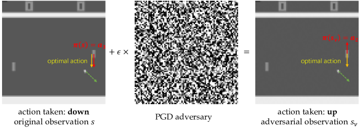
Figure 1: An example of state adversary in DQN. While the adversary disrupts the policy executed by DQN, it does not affect the optimal action prescribed by the Bellman optimal policy. This observation leads us to examine two critical issues: whether the Bellman optimal policy serves as the ORP, and why vanilla DQN trained with Bellman error fails to achieve robustness.

Given a general adversary, we observe that the true state $s$ and the perturbed observation $s_{\nu}$ typically share the same optimal action in practice. This observation, illustrated in Figure 1 and Appendix A, suggests that the Bellman optimal policy is inherently robust. We explore this by theoretically analyzing the effects of adversarial perturbations on the optimal action. We then define the intrinsic state neighborhood as the set of states for which the optimal action remains consistent.

Definition 1 (Intrinsic State Neighborhood)

Given an SA-MDP, let $Q^{*}$ denote the Bellman optimal $Q$ function derived from the Bellman optimality equations. The intrinsic state neighborhood for any state $s$ is defined as the following:

$$B^{*}(s):=\left\{s^{\prime}\in\mathcal{S}|s^{\prime}\in B(s),\ \mathop{\arg\max}_{a}Q^{*}(s^{\prime},a)=\mathop{\arg\max}_{a}Q^{*}(s,a)\right\}.$$

Without loss of generality, we assume that the adversary perturbation set is an $\epsilon$-neighborhood, defined as $B_{\epsilon}(s)=\left\{\|s^{\prime}-s\|\leq\epsilon\right\}$ for convenience. Note that our following theorems and proofs can be extended to general cases.

Furthermore, we characterize the states where the standard state neighborhood differs from the intrinsic neighborhood and show that such states are rare in real environments. This finding underpins the ISA-MDP formulation that we present later.

Theorem 2 (Sparse Difference Between Intrinsic and Standard Neighborhood)

For any MDP $\mathcal{M}$, let $\mathcal{S}_{nu}$ denote the state set where the optimal action is not unique, i.e., $\mathcal{S}_{nu}=\left\{s\in\mathcal{S}|\mathop{\arg\max}_{a}Q^{*}(s,a)\text{ is not a singleton}\right\}$. Given $\epsilon>0$, let $\mathcal{S}_{nin}$ denote the set of states where the intrinsic state $\epsilon$-neighborhood is not the same as the $\epsilon$-neighborhood, i.e., $\mathcal{S}_{nin}=\left\{s\in\mathcal{S}|B_{\epsilon}(s)\neq B^{*}_{\epsilon}(s)\right\}$. Then, we have that

$$\mathcal{S}_{nin}\subseteq\mathcal{S}_{nu}\cup\mathcal{S}_{0}+B_{\epsilon},$$

where $\mathcal{S}_{0}$ is the set of discontinuous points that cause the optimal action to change, i.e., $\mathcal{S}_{0}=\{s\in S|\forall\ \epsilon_{1}>0,\exists\ s^{\prime}\in B_{\epsilon_{1}}(s),\text{s.t. }\arg\max_{a}Q^{*}(s^{\prime},a)\neq\arg\max_{a}Q^{*}(s,a)\}\cap\{s\in S|\exists\ a\in\mathcal{A},\text{s.t. }Q^{*}(s,a)\ \text{is not continuous at}\ s\}$.

The proof of Theorem 2 is provided in Appendix B.1. In practice, the set $\mathcal{S}_{nu}$ is nearly empty in most complex environments, and $\mathcal{S}_{0}$ consists of rare and special discontinuous points of $Q^{*}$. Theorem 2 essentially shows that for intricate tasks, $\mathcal{S}_{nin}$ is a quite small set, with the measure $m(\mathcal{S}_{nin})$ being approximately $O(\epsilon^{d})$, where $m(A)$ represents the measure of set $A$ and $d$ is the dimension of the state space. For example, in certain natural environments, the reward function and transition dynamics are smooth, especially in continuous control tasks where the transition dynamics come from some physical laws. In these scenarios, the value and action-value functions are continuous, making $\mathcal{S}_{0}$ an empty set. Beyond smooth environments, many tasks can be modeled with sparse rewards. In these cases, the value and action-value functions are almost everywhere continuous, indicating that $\mathcal{S}_{0}$ is a set of zero measures. Further insights and stronger conclusions are provided in Appendix B.1 under more stringent conditions.

These findings and analysis motivate the development of the ISA-MDP formulation. Firstly, we introduce the concept of intrinsic adversaries.

Definition 3 (Intrinsic Adversary)

The intrinsic adversary $\nu_{I}:\mathcal{S}\rightarrow\mathcal{S},\ s\mapsto\nu_{I}(s)\in B^{*}(s)$ can perturb any state $s$ to a state $s_{\nu}:=\nu_{I}(s)$ within its intrinsic state neighborhood.

Building upon this definition, we formulate the intrinsic state-adversarial MDP.

Definition 4 (Intrinsic State-adversarial Markov Decision Process (ISA-MDP))

An intrinsic state-adversarial MDP is defined by the tuple $\left(\mathcal{S},\mathcal{A},r,\mathbb{P},\gamma,\mu_{0},B^{*},\nu_{I}\right)$, where the allowable perturbation set $B^{*}:\mathcal{S}\rightarrow 2^{\mathcal{S}}$ is the intrinsic state neighborhood as characterized in Definition 1, and $\nu_{I}$ is the intrinsic adversary defined in Definition 3.

While ISA-MDP can be seen as a more special characterization of SA-MDP with the intrinsic adversary, Theorem 2 inherently showcases that the difference between ISA-MDP and SA-MDP is negligible in complex environments, making ISA-MDP applicable in any scenario where SA-MDP is used.

4.2 Consistent Optimal Robust Policy

To establish the relation between the optimal $Q$-function before and after the perturbation, we propose a consistent adversarial robust (CAR) operator.

Definition 5 (Consistent Adversarial Robust (CAR) Operator $\mathcal{T}_{car}$)

Given an SA-MDP, the CAR operator is $\mathcal{T}_{car}:L^{p}\left(\mathcal{S}\times\mathcal{A}\right)\rightarrow L^{p}\left(\mathcal{S}\times\mathcal{A}\right)$,

$$\left(\mathcal{T}_{car}Q\right)(s,a)=r(s,a)+\gamma\mathbb{E}_{s^{\prime}\sim\mathbb{P}(\cdot|s,a)}\left[\min_{s^{\prime}_{\nu}\in B(s^{\prime})}Q\left(s^{\prime},\mathop{\arg\max}_{a_{s^{\prime}_{\nu}}}Q\left(s^{\prime}_{\nu},a_{s^{\prime}_{\nu}}\right)\right)\right].$$

However, $\mathcal{T}_{car}$ is not contractive (shown in Appendix B.2.1), so we cannot directly ensure the existence of a fixed point through contraction mapping. Fortunately, Theorem 6 demonstrates that within the ISA-MDP, $\mathcal{T}_{car}$ has a fixed point, which corresponds to the optimal adversarial action-value function $Q^{\pi^{*}\circ\nu^{*}(\pi^{*})}$.

Theorem 6 (Relation between $Q^{*}$ and $Q^{\pi^{*}\circ\nu^{*}(\pi^{*})}$)

• If the optimal adversarial action-value function $Q^{\pi^{*}\circ\nu^{*}(\pi^{*})}$ under the strongest adversary exists for all $s\in\mathcal{S}$ and $a\in\mathcal{A}$, then it is the fixed point of CAR operator.

• Within the ISA-MDP, $Q^{*}$ is the fixed point of CAR operator $\mathcal{T}_{car}$. Furthermore, $Q^{*}$ is the optimal adversarial action-value function under the strongest adversary, i.e., $Q^{*}(s,a)=Q^{\pi^{*}\circ\nu^{*}(\pi^{*})}(s,a)$, for all $s\in\mathcal{S}$ and $a\in\mathcal{A}$.

Remark 7

Note that the outer minimization and inner maximization operations in Definition 5 do not constitute a standard minimax problem because their objectives differ, resulting in a bilevel optimization problem. Generally, the minimization and maximization operations cannot be swapped. However, they can be swapped if $\mathop{\arg\max}_{a_{s^{\prime}_{\nu}}}Q\left(s^{\prime}_{\nu},a_{s^{\prime}_{\nu}}\right)$ is a singleton for all $s^{\prime}_{\nu}\in B(s^{\prime})$, which is a mild condition in our training. Additionally, we verify that $Q^{*}$ is still the fixed point of the operator after swapping.

On this basis, it can be derived from Theorem 6 that within the ISA-MDP, the greedy policy $\pi^{*}(s):=\mathop{\arg\max}_{a}Q^{*}(s,a)$, for all $s\in\mathcal{S}$, is exactly the ORP.

Corollary 8 (Existence of ORP)

Within the ISA-MDP, there exists a deterministic and stationary policy $\pi^{*}$ which satisfies $V^{\pi^{*}\circ\nu^{*}(\pi^{*})}(s)\geq V^{\pi\circ\nu^{*}(\pi)}(s)$ and $Q^{\pi^{*}\circ\nu^{*}(\pi^{*})}(s,a)\geq Q^{\pi\circ\nu^{*}(\pi)}(s,a)$, for all $\pi\in\Pi$, $s\in\mathcal{S}$ and $a\in\mathcal{A}$.

Theorem 6 and Corollary 8, whose proofs are provided in Appendix B.2.2, demonstrate that within the ISA-MDP, the ORP against the strongest adversary is equivalent to Bellman optimal policy derived from Bellman optimality equations. This finding indicates that the objectives in both natural and adversarial environments are aligned, as further supported by our experiment results in Figure 2, whose detailed illustrations are provided in Section 7.2.

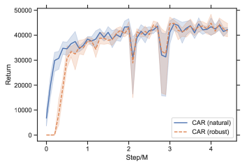
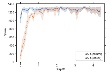
RoadRunner

BankHeist

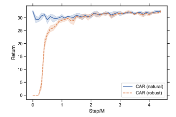
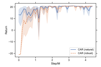
Freeway

Pong

Figure 2: Episode rewards of CAR-DQN agents with and without 10-step PGD attacks on 4 Atari games and 5 random seeds. As evidenced by the overlap of the two curves, CAR-DQN achieves the consistency between Bellman optimal policy and ORP.

Furthermore, we investigate the convergence of $\mathcal{T}_{car}$ in a smooth environment. We find that within the ISA-MDP, the fixed point iterations of $\mathcal{T}_{car}$ at least converge to a sub-optimal solution that is close to $Q^{*}$. The detailed proof of Theorem 9 and the formal definition of $\left(L_{r},L_{\mathbb{P}}\right)$-smooth environments are presented in Appendix B.2.3.

Theorem 9 (Convergence of CAR Operator $\mathcal{T}_{car}$)

Suppose the environment is $\left(L_{r},L_{\mathbb{P}}\right)$-smooth and suppose $Q_{0}$ and $r$ are uniformly bounded, i.e. $\exists\ M_{Q_{0}},M_{r}>0$ such that $\left|Q_{0}(s,a)\right|\leq M_{Q_{0}},\ \left|r(s,a)\right|\leq M_{r},\ \forall s\in\mathcal{S},a\in\mathcal{A}$. Let $Q^{*}$ denote the Bellman optimal Q-function and $Q_{k+1}=\mathcal{T}_{car}Q_{k}=\mathcal{T}_{car}^{k+1}Q_{0}$ for all $k\in\mathbb{N}$. Within the ISA-MDP, we have

$$\|Q_{k+1}-Q^{*}\|_{\infty}\leq\gamma^{k+1}\|Q_{0}-Q^{*}\|_{\infty}+\gamma^{k+1}D_{Q_{0}}+\frac{2\gamma\epsilon}{1-\gamma}L_{\mathcal{T}_{car}},$$

where $D_{Q_{0}}=2\max_{s,a}\max_{s_{\nu}\in B_{\epsilon}(s)}\max_{a}\left|Q_{0}\left(s,a\right)-Q_{0}\left(s_{\nu},a\right)\right|$ is a constant relating to the local continuity of initial $Q_{0}$, $L_{\mathcal{T}_{car}}=L_{r}+\gamma C_{Q_{0}}L_{\mathbb{P}}$ and $C_{Q_{0}}=\max\left\{M_{Q_{0}},\frac{M_{r}}{1-\gamma}\right\}$.

Given that the Bellman optimal policy doubles as the ORP, we further investigate the reasons behind the vulnerability of DRL agents. Despite aiming for the Bellman optimal policy, why do traditional reinforcement learning methods exhibit poor robustness? In the following section, we address this issue by examining the natural performance and robustness of policies across various measurement errors in action-value function and probability spaces.

5 Robustness of Policy with Tiny k-measurement Error

In this section, we examine the adversarial robustness of value-based and policy-based reinforcement learning methods with different measurements, identifying the significance of minimizing infinity measurement error to achieve the optimal robust policy.

5.1 Policy Robustness under Bellman p-error in Action-value Function Space

We investigate the stability of policies across various Banach spaces for value-based reinforcement learning methods and highlight the necessity of optimizing Bellman infinity-error to achieve the optimal robust policy. Firstly, in Subsection 5.1.1, we demonstrate the necessity of the $L^{\infty}$-norm for measuring $\|Q_{\theta}-Q^{*}\|$. Next, in Subsection 5.1.2, we identify the critical role of Bellman infinity-error in ensuring the stability of Bellman optimality equations. Finally, in Subsection 5.1.3, we extend these theoretical results to deep Q-learning, accounting for the practical sampling process.

5.1.1 Necessity of Infinity Norm in Action-value Function Space for Adversarial Robustness

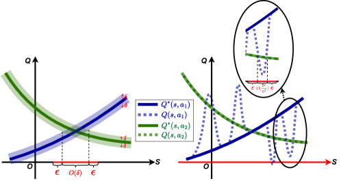
Figure 3: Examples of adversarial robustness for $Q$ satisfying $\|Q-Q^{*}\|_{p}\leq\delta$. Given a perturbation radius $\epsilon$, the red line represents the set $\mathcal{S}_{adv}^{Q}$, in which states have adversarial states. The left panel depicts the case of $p=\infty$. In this scenario, all such $Q$ functions are distributed within the shadow area, with the measure of $\mathcal{S}_{adv}^{Q}$ being a small value, approximately $2\epsilon+O\left(\delta\right)$, indicating good robustness. In contrast, the right panel shows that for $1\leq p<\infty$, there always exists a $Q$ function such that $\mathcal{S}_{adv}^{Q}=\mathcal{S}$, indicating poor robustness.

Let $Q_{\theta}$ denote a parameterized $Q$-function. Theoretically, value-based RL training requires minimizing $\left\|Q_{\theta}-Q^{*}\right\|_{\mathcal{B}}$, where $\mathcal{B}$ is a Banach space. When $\|Q_{\theta}-Q^{*}\|_{\mathcal{B}}$ equals zero, $Q_{\theta}$ perfectly matches $Q^{*}$. However, in practice, achieving this perfect match is challenging due to limitations such as the representation capacity of neural networks and the convergence issues in optimization algorithms. Given these practical constraints, we examine the properties of $Q_{\theta}$ when the $\left\|Q_{\theta}-Q^{*}\right\|_{\mathcal{B}}$ is a small positive value across different Banach spaces $\mathcal{B}$. This analysis underscores the importance of selecting appropriate norm spaces in ensuring adversarial robustness for value-based reinforcement learning methods.

We study the adversarial robustness of the greedy policy derived from $Q$ when $0<\left\|Q-Q^{*}\right\|_{p}=\delta\ll 1$ for different $L^{p}$ spaces. Given a function $Q$, let $\mathcal{S}^{Q}_{sub}$ denote the set of states where the greedy policy according to $Q$ is suboptimal, i.e.,

$$\mathcal{S}^{Q}_{sub}=\{s|Q^{*}(s,\mathop{\arg\max}_{a}Q(s,a))<\max_{a}Q^{*}(s,a)\}.$$

Note that the smaller set $\mathcal{S}^{Q}_{sub}$ indicates better performance in natural environments without adversarial attacks. For a given perturbation budget $\epsilon$, let $\mathcal{S}^{Q,\epsilon}_{adv}$ denote the set of states within whose $\epsilon$-neighborhood there exists the adversarial state, i.e.,

$$\mathcal{S}^{Q,\epsilon}_{adv}=\{s|\exists s_{\nu}\in B_{\epsilon}(s),\text{s.t. }Q^{*}(s,\mathop{\arg\max}_{a}Q(s_{\nu},a))<\max_{a}Q^{*}(s,a)\}.$$

The smaller the set $\mathcal{S}^{Q,\epsilon}_{adv}$, the stronger the adversarial robustness in the worst case. In addition, note that $\mathcal{S}_{sub}^{Q}=\mathcal{S}_{adv}^{Q,0}$. Furthermore, our investigation can be understood as a mathematical study of when it holds that $\lim_{\epsilon\rightarrow 0}\mathcal{S}_{adv}^{Q,\epsilon}=\mathcal{S}_{adv}^{Q,0}$, whose establishment indicates that the natural performance is aligned with the adversarial robustness in the worst case.

Theorem 10 (Necessity of the $L^{\infty}$ Space for Adversarial Robustness)

There exists an MDP instance such that the following statements hold.

• For any $1\leq p<\infty$ and $\delta>0$, there exists a function $Q\in L^{p}\left(\mathcal{S}\times\mathcal{A}\right)$ satisfying $\|Q-Q^{*}\|_{p}\leq\delta$ such that $m\left(\mathcal{S}^{Q}_{sub}\right)=O(\delta)$ yet $m\left(\mathcal{S}^{Q,\epsilon}_{adv}\right)=m\left(\mathcal{S}\right)$.

• There exists a $\bar{\delta}>0$ such that for any $0<\delta\leq\bar{\delta}$, and any function $Q\in L^{\infty}\left(\mathcal{S}\times\mathcal{A}\right)$ satisfying $\|Q-Q^{*}\|_{\infty}\leq\delta$, we have that $m\left(\mathcal{S}^{Q}_{sub}\right)=O(\delta)$ and $m\left(\mathcal{S}^{Q,\epsilon}_{adv}\right)=2\epsilon+O\left(\delta\right)$.

The proof of Theorem 10 is provided in Appendix C.1. The first statement indicates that when $\|Q-Q^{*}\|_{p}$ is small for $1\leq p<\infty$, there always exist adversarial examples near almost all states, resulting in quite poor robustness, even though the policy might exhibit excellent performance in a natural environment without adversarial attacks. This observation sheds light on the vulnerability of DRL agents, consistent with findings from various studies (Huang et al., 2017; Ilahi et al., 2021). Importantly, the second statement points out that minimizing $\|Q-Q^{*}\|$ in the $L^{\infty}$-norm space can mitigate this vulnerability, enabling the policy to achieve both natural performance and robustness. This insight motivates the optimization of $\|Q_{\theta}-Q^{*}\|_{\infty}$ in DRL algorithms. Intuitive examples of Theorem 10 are illustrated in Figure 3.

5.1.2 Stability of Bellman Optimality Equations

Unfortunately, it is infeasible to directly measure $\|Q_{\theta}-Q^{*}\|$ in practical DRL procedures due to the unknown nature of $Q^{*}$. Most value-based methods train $Q_{\theta}$ by optimizing the Bellman error $\|\mathcal{T}_{B}Q_{\theta}-Q_{\theta}\|_{\mathcal{B}^{\prime}}$, where $\mathcal{T}_{B}$ is the Bellman optimal operator:

$$\left(\mathcal{T}_{B}Q\right)(s,a)=r(s,a)+\gamma\mathbb{E}_{s^{\prime}\sim\mathbb{P}(\cdot\mid s,a)}\left[\max_{a^{\prime}\in\mathcal{A}}Q\left(s^{\prime},a^{\prime}\right)\right].$$

Similar to Theorem 10, we need to determine which Banach space $\mathcal{B}^{\prime}$ is the best for training DRL agents to minimize adversarial states. When $\|\mathcal{T}_{B}Q_{\theta}-Q_{\theta}\|_{\mathcal{B}^{\prime}}$ is zero, $Q_{\theta}$ is precisely $Q^{*}$. However, in practice, we can only optimize $\|\mathcal{T}_{B}Q_{\theta}-Q_{\theta}\|_{\mathcal{B}^{\prime}}$ to a small nonzero quantity. In this scenario, we discuss the conditions under which $\left\|Q_{\theta}-Q^{*}\right\|_{\mathcal{B}}$ can be controlled. To analyze this issue, we introduce the concept of functional equations stability, drawing on relevant research about physics-informed neural networks for partial differential equations (Wang et al., 2022).

Definition 11 (Stability of Functional Equations)

Given two Banach spaces $\mathcal{B}_{1}$ and $\mathcal{B}_{2}$, if there exist $\delta>0$ and $C>0$ such that for all $Q\in\mathcal{B}_{1}\cap\mathcal{B}_{2}$ satisfying $\|\mathcal{T}Q-Q\|_{\mathcal{B}_{1}}<\delta$, we have that $\|Q-Q^{*}\|_{\mathcal{B}_{2}}<C\|\mathcal{T}Q-Q\|_{\mathcal{B}_{1}}$, where $Q^{*}$ is the exact solution of this functional equation, then we say a nonlinear functional equation $\mathcal{T}Q=Q$ is $\left(\mathcal{B}_{1},\mathcal{B}_{2}\right)$-stable. For simplicity, we call that functional $\mathcal{T}$ is $\left(\mathcal{B}_{1},\mathcal{B}_{2}\right)$-stable.

Remark 12

This definition indicates that if $\mathcal{T}Q=Q$ is $\left(\mathcal{B}_{1},\mathcal{B}_{2}\right)$-stable, then $\|Q-Q^{*}\|_{\mathcal{B}_{2}}=O\left(\|\mathcal{T}Q-Q\|_{\mathcal{B}_{1}}\right)$, as $\|\mathcal{T}Q-Q\|_{\mathcal{B}_{1}}\longrightarrow 0$, $\forall\ Q\in\mathcal{B}_{1}\cap\mathcal{B}_{2}$.

The above Definition implies that if there exists a space $\mathcal{B}^{\prime}$ such that $\mathcal{T}_{B}$ is $\left(\mathcal{B}^{\prime},L^{\infty}\left(\mathcal{S}\times\mathcal{A}\right)\right)$-stable, then $\left\|Q_{\theta}-Q^{*}\right\|_{\infty}$ will be controlled when minimizing the Bellman error in $\mathcal{B}^{\prime}$ space. This will make DRL agents robust according to Theorem 10.(2). The following theorems illustrate the conditions that affect the stability and instability of $\mathcal{T}_{B}$ and provide guidance for selecting a suitable $\mathcal{B}^{\prime}$.

Theorem 13 (Stable and Unstable Properties of $\mathcal{T}_{B}$ in $L^{p}$ Spaces)

• For any MDP $\mathcal{M}$, let $C_{\mathbb{P},p}:=\sup_{(s,a)\in\mathcal{S}\times\mathcal{A}}\left\|\mathbb{P}(\cdot\mid s,a)\right\|_{L^{\frac{p}{p-1}}\left(\mathcal{S}\right)}$. Assume $p$ and $q$ satisfy the following conditions:

  $$C_{\mathbb{P},p}<\frac{1}{\gamma};\quad p\geq\max\left\{1,\frac{\log\left(\left|\mathcal{A}\right|\right)+\log\left(\mu\left(\mathcal{S}\right)\right)}{\log\frac{1}{\gamma C_{\mathbb{P},p}}}\right\};\quad p\leq q\leq\infty.$$

  Then, Bellman optimality equation $\mathcal{T}_{B}Q=Q$ is $\left(L^{q}\left(\mathcal{S}\times\mathcal{A}\right),L^{p}\left(\mathcal{S}\times\mathcal{A}\right)\right)$-stable.

• There exists an MDP such that for all $1\leq q<p\leq\infty$, the Bellman optimality equation $\mathcal{T}_{B}Q=Q$ is not $\left(L^{q}\left(\mathcal{S}\times\mathcal{A}\right),L^{p}\left(\mathcal{S}\times\mathcal{A}\right)\right)$-stable.

Remark 14

Note that we have proved a stronger conclusion than stability because the stable property holds for all $Q$ rather than for $Q$ satisfying $\|\mathcal{T}Q-Q\|_{\mathcal{B}_{1}}\longrightarrow 0$.

The proofs of Theorem 13 are shown in Appendices C.2 and C.3. We note that $\lim_{p\rightarrow\infty}C_{\mathbb{P},p}=1<\frac{1}{\gamma}$, so the first condition holds when $p$ is sufficiently large. The second condition indicates that $p$ is relevant to the size of the state and action spaces, and the third condition reveals that stability is achievable when $q$ is larger than $p$. Consequently, we have that $\mathcal{T}_{B}$ is $\left(L^{\infty}\left(\mathcal{S}\times\mathcal{A}\right),L^{\infty}\left(\mathcal{S}\times\mathcal{A}\right)\right)$-stable. Therefore, to achieve adversarial robustness, we can optimize DRL agents in space $\mathcal{B}^{\prime}=L^{\infty}\left(\mathcal{S}\times\mathcal{A}\right)$. Moreover, $\mathcal{B}^{\prime}$ cannot be $L^{q}\left(\mathcal{S}\times\mathcal{A}\right)$ for any $1\leq q<\infty$, as stated in Theorem 13.(2).

5.1.3 Stability of Deep Q-learning

Our theoretical analysis has shown that training a deep Q-network (DQN) by minimizing the Bellman error in $L^{\infty}$ space is feasible for achieving the ORP. In this subsection, we further examine the stability of DQN by considering the practical sampling process.

Given an MDP $\mathcal{M}$, define the state-action visitation distribution $d_{\mu_{0}}^{\pi}$ as the following:

$$d_{\mu_{0}}^{\pi}(s,a)=\mathbb{E}_{s_{0}\sim\mu_{0}(\cdot),s_{t}\sim\mathbb{P}(\cdot|s_{t-1},a_{t-1}),a_{t}\sim\pi(\cdot|s_{t})}\left[(1-\gamma)\sum_{t=0}^{\infty}\gamma^{t}\mathbb{I}(s_{t}=s,a_{t}=a)\right].$$

Deep Q-learning algorithms, such as DQN, utilize the following objective $\mathcal{L}(Q_{\theta};\pi_{\theta})$ based on interactions with the environment:

$$\mathcal{L}(Q_{\theta};\pi_{\theta})=\mathbb{E}_{(s,a)\sim d_{\mu_{0}}^{\pi_{\theta}}}\left|\mathcal{T}_{B}Q_{\theta}(s,a)-Q_{\theta}(s,a)\right|.$$

The theoretical analysis of functional equations stability can be extended to $\mathcal{L}(Q_{\theta};\pi_{\theta})$ by incorporating the sampling probability into a seminorm.

Definition 15 ($(p,d_{\mu_{0}}^{\pi})$-seminorm)

Given a policy $\pi$, a function $f:\mathcal{S}\times\mathcal{A}\rightarrow\mathbb{R}$ and $1\leq p\leq\infty$, if $d_{\mu_{0}}^{\pi}$ is a probability density function, we define the $(p,d_{\mu_{0}}^{\pi})$-seminorm as the following, which satisfies the absolute homogeneity and triangle inequality:

$$\left\|f\right\|_{p,d_{\mu_{0}}^{\pi}}:=\left\|d_{\mu_{0}}^{\pi}f\right\|_{p}=\left(\int_{(s,a)\in\mathcal{S}\times\mathcal{A}}\left|d_{\mu_{0}}^{\pi}(s,a)f(s,a)\right|^{p}d\mu(s,a)\right)^{\frac{1}{p}}.$$

We further analysis the properties of this seminorm in Appendix D.1. Note that the $(p,d_{\mu_{0}}^{\pi})$-seminorm becomes a norm if $d_{\mu_{0}}^{\pi}(s,a)>0$ almost everywhere for $(s,a)\in\mathcal{S}\times\mathcal{A}$. Based on this definition, the deep Q-learning objective $\mathcal{L}(Q_{\theta};\pi_{\theta})$ can be expressed as

$$\mathcal{L}(Q_{\theta};\pi_{\theta})=\left\|\mathcal{T}_{B}Q_{\theta}-Q_{\theta}\right\|_{1,d_{\mu_{0}}^{\pi_{\theta}}}.$$

Similar to Theorem 13, we prove that the objective $\mathcal{L}(Q_{\theta};\pi_{\theta})$ cannot ensure robustness, while $(\infty,d_{\mu_{0}}^{\pi})$-seminorm is necessary for adversarial robustness.

Theorem 16 (Stable and Unstable Properties of $\mathcal{T}_{B}$ in $(p,d_{\mu_{0}}^{\pi})$-seminorm Spaces)

• For any MDP $\mathcal{M}$ and fixed policy $\pi$, assume $C_{d_{\mu_{0}}^{\pi}}:=\inf_{(s,a)\in\mathcal{S}\times\mathcal{A}}d_{\mu_{0}}^{\pi}(s,a)>0$ and assume $p$ and $q$ satisfy the following conditions:

  $$C_{\mathbb{P},p}<\frac{1}{\gamma};\quad p\geq\max\left\{1,\frac{\log\left(\left|\mathcal{A}\right|\right)+\log\left(\mu\left(\mathcal{S}\right)\right)}{\log\frac{1}{\gamma C_{\mathbb{P},p}}}\right\};\quad p\leq q\leq\infty,$$

  where $C_{\mathbb{P},p}:=\sup_{(s,a)\in\mathcal{S}\times\mathcal{A}}\left\|\mathbb{P}(\cdot\mid s,a)\right\|_{L^{\frac{p}{p-1}}\left(\mathcal{S}\right)}$. Then, Bellman optimality equation $\mathcal{T}_{B}Q=Q$ is $\left(L^{q,d_{\mu_{0}}^{\pi}}\left(\mathcal{S}\times\mathcal{A}\right),L^{p}\left(\mathcal{S}\times\mathcal{A}\right)\right)$-stable.

• There exists an MDP $\mathcal{M}$ such that for all $\pi$ satisfying $M_{d_{\mu_{0}}^{\pi}}:=\sup_{(s,a)\in\mathcal{S}\times\mathcal{A}}d_{\mu_{0}}^{\pi}(s,a)<\infty$, Bellman optimality equation $\mathcal{T}_{B}Q=Q$ is not $\left(L^{q,d_{\mu_{0}}^{\pi}}\left(\mathcal{S}\times\mathcal{A}\right),L^{p}\left(\mathcal{S}\times\mathcal{A}\right)\right)$-stable, for all $1\leq q<p\leq\infty$.

Remark 17

Note that in a practical Q-learning scheme, we take the $\epsilon$-greedy policy for exploration. As a result, for any state-action pair $(s,a)$, we can visit it with positive probability, and thus the condition $C_{d_{\mu_{0}}^{\pi}}>0$ holds.

The proofs of Theorem 16 are provided in Appendix D.2, where a theorem with tighter bounds yet stringent conditions is also shown. We also investigate the stability when $d_{\mu_{0}}^{\pi}$ is a probability mass function in Appendices D.1 and D.3.

5.2 Policy Robustness under k-measurement Error in Probability Space

We examine the adversarial robustness of policy-based reinforcement learning methods across different measurements in probability space, emphasizing the importance of optimizing infinity measurement error to attain the optimal robust policy. In Subsection 5.2.1, we reformulate the optimization objectives of REINFORCE and PPO as $1$-measurement errors, drawing on the operator view of policy gradient methods presented by Ghosh et al. (2020). In Subsection 5.2.2, we demonstrate the vulnerability of non-infinity measurement errors and establish robustness guarantee under infinity measurement error.

5.2.1 Probability Measurement Formulation for Policy-based Reinforcement Learning

We reformulate the optimization objectives of two key policy-based reinforcement learning methods, REINFORCE (Williams, 1992) and PPO (Schulman et al., 2017), as the discrepancy between two probability distributions under $1$-measurement.

Firstly, we define a $k$-measurement in probability space to describe the discrepancy between two probability distributions.

Definition 18 ($k$-measurement in Probability Space)

Given any probability distributions $\omega(\cdot)\in\Delta(\mathcal{S})$ and $p(\cdot|s),q(\cdot|s)\in\Delta(\mathcal{A})$ for all $s\in\mathcal{S}$, the $k$-measurement with f-divergence between $p$ and $q$ under $\omega$ is defined as the following:

$$\mathcal{D}_{k,f}^{\omega}\left(p\|q\right):=\left\|\omega\mathcal{D}_{f}\left(p\|q\right)\right\|_{k}=\left(\int_{s\in\mathcal{S}}\left|\omega(s)\mathcal{D}_{f}\left(p(\cdot|s)\|q(\cdot|s)\right)\right|^{k}d\mu(s)\right)^{\frac{1}{k}},$$

where $\mathcal{D}_{f}$ represents the f-divergence in policy space.

Remark 19

Note that $\mathcal{D}_{k,f}^{\omega}$ is not a distance due to the asymmetrical nature of f-divergence.

Given an MDP $\mathcal{M}$, define the state visitation distribution $d_{\mu_{0}}^{\pi}$ as the following:

$$d_{\mu_{0}}^{\pi}(s)=\mathbb{E}_{s_{0}\sim\mu_{0}(\cdot),a_{t-1}\sim\pi(\cdot|s_{t-1}),s_{t}\sim\mathbb{P}(\cdot|s_{t-1},a_{t-1})}\left[(1-\gamma)\sum_{t=0}^{\infty}\gamma^{t}\mathbb{I}(s_{t}=s)\right].$$

In the following text, if there is no ambiguity, we will abbreviate $d_{\mu_{0}}^{\pi}$ to $d^{\pi}$.

Probability Measurement Formulation of REINFORCE.

REINFORCE is one of the most fundamental policy-based methods and updates according to the policy gradient theorem. Its update can be formulated as the following:

$$\theta_{t+1}=\theta_{t}+\eta_{t}\mathbb{E}_{s\sim d^{\pi_{t}}(\cdot),a\sim\pi_{t}(\cdot|s)}\left[Q^{\pi_{t}}(s,a)\nabla_{\theta}\log\pi_{\theta}(a|s)\Big{|}_{\theta=\theta_{t}}\right],$$

where $\pi_{\theta_{t}}$ is abbreviated as $\pi_{t}$. If $Q^{\pi}(s,a)$ are positive for all $(s,a)\in\mathcal{S}\times\mathcal{A}$, the above equation can be interpreted as performing a gradient step for the optimization problem:

$$\min_{\pi_{\theta}\in\Pi}\mathcal{D}_{1,\operatorname{KL}}^{\mu_{t}}\left(\varphi_{t}\|\pi_{\theta}\right),$$

where probability distributions $\varphi_{t}$ and $\mu_{t}$ are as follows, respectively:

$$\varphi_{t}(a|s)=\frac{1}{V^{\pi_{t}}(s)}Q^{\pi_{t}}(s,a)\pi_{t}(a|s),\quad\mu_{t}(s)=\frac{1}{\mathbb{E}_{s\sim d^{\pi_{t}}(\cdot)}\left[V^{\pi_{t}}(s)\right]}d^{\pi_{t}}(s)V^{\pi_{t}}(s).$$

It can be explained as iteratively approximating an improved policy $\varphi_{t}$ based on value functions by optimizing a $1$-measurement with the forward KL-divergence.

Probability Measurement Formulation of PPO.

PPO is one of the most widely used policy-based methods and often incorporates an entropy bonus with a coefficient $\beta>0$. PPO can be viewed as performing a gradient step for the following optimization problem:

$$\min_{\pi_{\theta}\in\Pi}\mathcal{D}_{1,\operatorname{KL}}^{\mu_{t}}\left(\operatorname{clip}(\pi_{\theta})\|\varphi_{t}\right),$$

where probability distributions $\varphi_{t}$ and $\mu_{t}$ are as follows, respectively:

$$\varphi_{t}(a|s)=\frac{\exp\left(\beta A^{\pi_{t}}(s,a)\right)}{\sum_{a^{\prime}}\exp\left(\beta A^{\pi_{t}}(s,a^{\prime})\right)},\quad\mu_{t}(s)=d^{\pi_{t}}(s).$$

Similarly, it can be understood as iteratively approximating an improved policy $\varphi_{t}$ based on advantage functions by minimizing a $1$-measurement with the reversed KL-divergence. This formulation results in the update:

$$\pi_{t+1}=\mathop{\arg\max}_{\pi_{\theta}}\mathbb{E}_{s\sim d^{\pi_{t}}(\cdot)}\left[\sum_{a}\pi_{\theta}(a|s)A^{\pi_{t}}(s,a)-\frac{1}{\beta}\sum_{a}\pi_{\theta}(a|s)\log\pi_{\theta}(a|s)\right],$$

where the clipping operator is omitted for readability.

5.2.2 Necessity of Infinity Measurement in Probability Space for Adversarial Robustness

When the value of $\mathcal{D}_{k,\operatorname{KL}}^{\mu_{t}}$ vanishes, $\pi_{\theta}$ is exactly the improved policy $\varphi_{t}$. However, this is not achievable due to practical constraints. Therefore, we investigate the approximation properties when the $\mathcal{D}_{k,\operatorname{KL}}^{\mu_{t}}$ is a small but nonzero value for different $k$. This examination highlights the significance of utilizing suitable measurements for guaranteeing adversarial robustness in policy-based reinforcement learning methods.

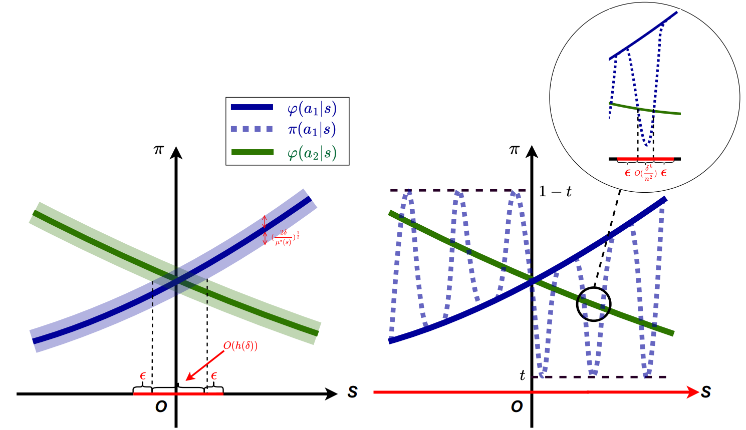
Figure 4: Examples of adversarial robustness for the policy $\pi$ satisfying $\mathcal{D}_{k,\operatorname{KL}}^{\mu}\left(\varphi\|\pi\right)\leq\delta$. Given a perturbation radius $\epsilon$, the red line represents the set $\mathcal{S}_{adv}^{\pi,\epsilon}$, which consists of states with adversarial states. In the left panel, we depict the case of $k=\infty$. In this scenario, all such policies $\pi$ are distributed within the shadow area, with the measure of $\mathcal{S}_{adv}^{\pi,\epsilon}$ being a small value, approximately $2\epsilon+O\left(h(\delta)\right)$, indicating good robustness. In contrast, the right panel illustrates that for $1\leq k<\infty$, there always exists $\pi$ such that $\mathcal{S}_{adv}^{\pi,\epsilon}=\mathcal{S}$ in the worst case, indicating poor robustness.

Given a policy $\pi$ and a perturbation budget $\epsilon$, let $\mathcal{S}_{sub}^{\pi}$ represent the set of states where the greedy policy according to $\pi$ is suboptimal:

$$\mathcal{S}_{sub}^{\pi}=\left\{s\left|Q^{*}(s,\mathop{\arg\max}_{a}\pi(a|s))<\max_{a}Q^{*}(s,a)\right.\right\}.$$

The smaller set $\mathcal{S}_{sub}^{\pi}$ signifies better natural performance. Given a perturbation budget $\epsilon$, $\mathcal{S}_{adv}^{\pi,\epsilon}$ denotes the state set within whose $\epsilon$-neighborhood there exists the adversarial state:

$$\mathcal{S}_{adv}^{\pi,\epsilon}=\left\{s\left|\exists\ s_{\nu}\in B_{\epsilon}(s),\text{s.t. }Q^{*}(s,\mathop{\arg\max}_{a}\pi(a|s_{\nu}))<\max_{a}Q^{*}(s,a)\right.\right\}.$$

The smaller set $\mathcal{S}_{adv}^{\pi,\epsilon}$ means stronger worst-case adversarial robustness. In addition, we note that $\mathcal{S}_{sub}^{\pi}=\mathcal{S}_{adv}^{\pi,0}$. From this perspective, our analysis can be understood as a mathematical study of when it holds that $\lim_{\epsilon\rightarrow 0}\mathcal{S}_{adv}^{\pi,\epsilon}=\mathcal{S}_{adv}^{\pi,0}$, showcasing that the natural performance and the adversarial robustness in the worst case are consistent. Denote that $\pi^{*}$ as the greedy policy according to the Bellman optimal $Q$-function and $\mu^{*}(s):=d^{\pi^{*}}(s),\ \forall\ s\in\mathcal{S}$.

We first demonstrate that small $k$-measurement errors for any $1\leq k<\infty$ may ensure the natural performance but can lead to complete vulnerability in the worst case.

Theorem 20 (Vulnerability of Non-infinity Measurement Errors)

There exists an MDP such that the following statement holds. Let $\varphi$ be a policy from the policy family $\mathcal{F}=\left\{\varphi\left|\mathop{\arg\max}_{a}\varphi(a|s)=\mathop{\arg\max}_{a}\pi^{*}(a|s)\right.\right\}$. For any $\epsilon>0$, $1\leq k<\infty$, $\delta>0$ and any state distribution $\mu$, there exists a policy $\pi$ satisfying $\mathcal{D}_{k,\operatorname{KL}}^{\mu}\left(\varphi\|\pi\right)\leq\delta$ and $\mathcal{D}_{k,\operatorname{KL}}^{\mu}\left(\pi\|\varphi\right)\leq\delta$, such that $m\left(\mathcal{S}_{sub}^{\pi}\right)=O(\delta)$ but $m\left(\mathcal{S}_{adv}^{\pi,\epsilon}\right)=m(\mathcal{S})$.

Fortunately, we find that policies with small infinity measurement errors can guarantee both natural and robust performance.

Theorem 21 (Robustness Guarantee under Infinity Measurement Error)

For any MDP and state distribution $\mu>0$, let $S_{\delta}=\{s\mid\exists\ a,a^{\prime}\in\mathcal{A},\ \text{s.t.}\ |\varphi(a|s)-\varphi(a^{\prime}|s)|\leq 2\sqrt{\frac{2\delta}{\mu(s)}}\}$ and $h(\delta)=\mu(S_{\delta})$. Then $h(\delta)$ is a monotonic function with $h(0)=0$. Furthermore, let $\varphi$ be a policy from the policy class $\mathcal{F}=\left\{\varphi\mid\mathop{\arg\max}_{a}\varphi(a|s)=\mathop{\arg\max}_{a}\pi^{*}(a|s)\right\}$. If $S_{\delta}$ is the union of finite connected subsets, then for any $\epsilon,\delta>0$ and any policy $\pi$ satisfying $\mathcal{D}_{\infty,\operatorname{KL}}^{\mu}\left(\varphi\|\pi\right)\leq\delta$ or $\mathcal{D}_{\infty,\operatorname{KL}}^{\mu}\left(\pi\|\varphi\right)\leq\delta$, we have that $m\left(\mathcal{S}_{sub}^{\pi}\right)=O(h(\delta))$ and $m\left(\mathcal{S}_{adv}^{\pi,\epsilon}\right)=2\epsilon+O(h(\delta))$.

The proofs of Theorem 20 and 21 are presented in Appendix E, with intuitional examples illustrated in Figure 4. These findings underscore the necessity of using $\mathcal{D}_{\infty,\operatorname{KL}}^{\mu_{t}}$ as the objective for ensuring adversarial robustness in the worst case.

6 Consistent Adversarial Robust Reinforcement Learning

Our theoretical analysis reveals the potential of employing the infinity measurement error as the optimization objective to achieve the optimal robust policy. However, the exact computation of the infinity measurement is intractable due to the unknown environment dynamics and continuous state space. Therefore, we introduce the surrogate objective of the infinity measurement error and develop the Consistent Adversarial Robust Reinforcement Learning (CAR-RL) framework. This framework enhances both the natural and robust performance of agents. Furthermore, we apply CAR-RL to both the value-based DQN and the policy-based PPO algorithms, leading to CAR-DQN and CAR-PPO.

6.1 Consistent Adversarial Robust Deep Q-network

Inspired by Theorem 16, we propose the CAR-DQN to train robust DQN by minimizing the Bellman infinity-error $\|\mathcal{T}_{B}Q_{\theta}-Q_{\theta}\|_{\infty,d^{\pi_{\theta}}_{\mu_{0}}}$. This objective can be minimized using the following loss function (as derived in Appendix F.1):

$$\mathcal{L}_{car}(\theta)=\sup_{(s,a)\in\mathcal{S}\times\mathcal{A}}d_{\mu_{0}}^{\pi_{\theta}}(s,a)\max_{s_{\nu}\in B_{\epsilon}(s)}\left|\mathcal{T}_{B}Q_{\theta}(s_{\nu},a)-Q_{\theta}(s_{\nu},a)\right|,$$

where $\pi_{\theta}$ is the behavior policy associated with $Q_{\theta}$, typically an $\epsilon$-greedy policy derived from $Q_{\theta}$. Since interactions with the environment in an SA-MDP are based on the true state $s$ rather than the perturbed state $s_{\nu}$, it is not feasible to directly estimate $\mathcal{T}_{B}Q_{\theta}(s_{\nu},a)$. To address this, we exploit $\mathcal{T}_{B}Q_{\theta}(s,a)$ as a substitute, leading to the training objective:

$$\mathcal{L}_{car}^{train}(\theta)=\sup_{(s,a)\in\mathcal{S}\times\mathcal{A}}d_{\mu_{0}}^{\pi_{\theta}}(s,a)\max_{s_{\nu}\in B_{\epsilon}(s)}\left|\mathcal{T}_{B}Q_{\theta}(s,a)-Q_{\theta}(s_{\nu},a)\right|.$$

As shown in Theorem 22, this surrogate objective $\mathcal{L}_{car}^{train}$ effectively bounds $\mathcal{L}_{car}$, especially in smooth environments. We also define $\mathcal{L}_{car}^{diff}(\theta)$ as the following:

$$\mathcal{L}_{car}^{diff}(\theta)=\sup_{(s,a)\in\mathcal{S}\times\mathcal{A}}d_{\mu_{0}}^{\pi_{\theta}}(s,a)\max_{s_{\nu}\in B_{\epsilon}(s)}\left|\mathcal{T}_{B}Q_{\theta}(s_{\nu},a)-\mathcal{T}_{B}Q_{\theta}(s,a)\right|.$$

Theorem 22 (Bounding $\mathcal{L}_{car}$ with $\mathcal{L}_{car}^{train}$)

We have that

$$\left|\mathcal{L}_{car}^{train}(\theta)-\mathcal{L}_{car}^{diff}(\theta)\right|\leq\mathcal{L}_{car}(\theta)\leq\mathcal{L}_{car}^{train}(\theta)+\mathcal{L}_{car}^{diff}(\theta).$$

Further, suppose the environment is $\left(L_{r},L_{\mathbb{P}}\right)$-smooth and suppose $Q_{\theta}$ and $r$ are uniformly bounded, i.e. $\exists\ M_{Q},M_{r}>0$ such that $\left|Q_{\theta}(s,a)\right|\leq M_{Q},\ \left|r(s,a)\right|\leq M_{r}\ \forall s\in\mathcal{S},a\in\mathcal{A}$. If $M:=\sup_{\theta,(s,a)\in\mathcal{S}\times\mathcal{A}}d_{\mu_{0}}^{\pi_{\theta}}(s,a)<\infty$, then we have that

$$\mathcal{L}_{car}^{diff}(\theta)\leq C_{\mathcal{T}_{B}}\epsilon,$$

where $C_{\mathcal{T}_{B}}=L_{\mathcal{T}_{B}}M$, $L_{\mathcal{T}_{B}}=L_{r}+\gamma C_{Q}L_{\mathbb{P}}$ and $C_{Q}=\max\left\{M_{Q},\frac{M_{r}}{1-\gamma}\right\}$. The definition of $\left(L_{r},L_{\mathbb{P}}\right)$-smooth environment is shown in Appendix B.2.3.

The proofs of Theorem 22 are provided in Appendix F.1.1, which confirm that $\mathcal{L}_{car}^{train}(\theta)$ is a valid surrogate objective from the optimization perspective. This theorem also highlights a potential source of instability during robust training: if $\mathcal{L}_{car}^{train}(\theta)$ is minimized to a small value but remains less than $\mathcal{L}_{car}^{diff}(\theta)$, then the primary objective $\mathcal{L}_{car}(\theta)$ may tend to increase, indicating a potential training overfitting.

To make better use of batch samples and improve training efficiency, we introduce a soft version $\mathcal{L}_{car}^{soft}(\theta)$ of the CAR objective, denoted as $\mathcal{L}_{car}^{soft}(\theta)$ (derivation in Appendix F.1.2):

$$\mathcal{L}_{car}^{soft}(\theta)=\sum_{i\in\mathcal{\left|B\right|}}\alpha_{i}\max_{s_{\nu}\in B_{\epsilon}(s_{i})}\left|r_{i}+\gamma\max_{a^{\prime}}Q_{\bar{\theta}}(s_{i}^{\prime},a^{\prime})-Q_{\theta}(s_{\nu},a_{i})\right|,$$

where the weighting $\alpha_{i}$ is defined by the following probability distribution over a batch:

$$\alpha_{i}=\frac{e^{\frac{1}{\lambda}\max_{s_{\nu}}\left|r_{i}+\gamma\max_{a^{\prime}}Q_{\bar{\theta}}(s_{i}^{\prime},a^{\prime})-Q_{\theta}(s_{\nu},a_{i})\right|}}{\sum_{i\in\mathcal{\left|B\right|}}e^{\frac{1}{\lambda}\max_{s_{\nu}}\left|r_{i}+\gamma\max_{a^{\prime}}Q_{\bar{\theta}}(s_{i}^{\prime},a^{\prime})-Q_{\theta}(s_{\nu},a_{i})\right|}}.$$

Here, $\mathcal{B}$ represents a batch of transition pairs sampled from the replay buffer, $\bar{\theta}$ is the parameter of the target network, and $\lambda$ is the coefficient to control the level of softness.

6.2 Consistent Adversarial Robust Proximal Policy Optimization

Motivated by Theorems 20 and 21, we develop the CAR-PPO method to enhance the robustness of PPO. The objective of CAR-PPO is to optimize the infinity measurement error $\mathcal{D}_{\infty,\operatorname{KL}}^{\mu_{t}}\left(\operatorname{clip}(\pi_{\theta})\|\varphi_{t}\right)$. This is equivalent to minimizing the following loss function (as derived in Appendix F.2):

$$\mathcal{L}_{car}^{train}(\theta)=\sup_{s\in\mathcal{S}}\ d^{\pi_{t}}(s)\left(-\frac{1}{\beta}\mathcal{H}\left(\pi_{\theta}(\cdot|s)\right)-\min_{s_{\nu}\in B(s)}\mathbb{E}_{a\sim\pi_{t}(\cdot|s)}\left[g\left(\frac{\pi_{\theta}(a|s_{\nu})}{\pi_{t}(a|s)},A^{\pi_{t}}(a|s)\right)\right]\right),$$

where $\mathcal{H}(\cdot)$ represents the entropy, and the function $g(x,y)$ is defined as:

$$g(x,y)=\min\left\{x\cdot y,\operatorname{clip}\left(x,1-\eta,1+\eta\right)\cdot y\right\},$$

with $\eta$ being the clipping hyperparameter.

Furthermore, we approximate the objective $\mathcal{L}_{car}^{train}(\theta)$ by considering the practice sampling process. The approximate objective is defined as:

$$\mathcal{L}_{car}^{app}(\theta)=\frac{1}{|\mathcal{B}|}\max_{(s,a)\in\mathcal{B}}\left(-\frac{1}{\beta}\mathcal{H}\left(\pi_{\theta}(\cdot|s)\right)-\min_{s_{\nu}\in B(s)}g\left(\frac{\pi_{\theta}(a|s_{\nu})}{\pi_{t}(a|s)},A^{\pi_{t}}(a|s)\right)\right).$$

To effectively utilize each sample in a minibatch and improve training efficiency, we introduce a soft version $\mathcal{L}_{car}^{soft}(\theta)$ of the CAR objective $\mathcal{L}_{car}^{app}(\theta)$:

$$\mathcal{L}_{car}^{soft}(\theta)=\frac{1}{|\mathcal{B}|}\sum_{(s_{i},a_{i})\in\mathcal{B}}\alpha_{i}\left(-\frac{1}{\beta}\mathcal{H}\left(\pi_{\theta}(\cdot|s_{i})\right)-\min_{s_{\nu}\in B(s_{i})}g\left(\frac{\pi_{\theta}(a_{i}|s_{\nu})}{\pi_{t}(a_{i}|s_{i})},A^{\pi_{t}}(a_{i}|s_{i})\right)\right),$$

where the sample weighting $\alpha_{i}$ is defined by the following distribution over a minibatch:

$$\alpha_{i}=\frac{e^{\frac{1}{\lambda}\left(-\frac{1}{\beta}\mathcal{H}\left(\pi_{\theta}(\cdot|s_{i})\right)-\min_{s_{\nu}\in B(s_{i})}g\left(\frac{\pi_{\theta}(a_{i}|s_{\nu})}{\pi_{t}(a_{i}|s_{i})},A^{\pi_{t}}(a_{i}|s_{i})\right)\right)}}{\sum_{i\in\mathcal{\left|B\right|}}e^{\frac{1}{\lambda}\left(-\frac{1}{\beta}\mathcal{H}\left(\pi_{\theta}(\cdot|s_{i})\right)-\min_{s_{\nu}\in B(s_{i})}g\left(\frac{\pi_{\theta}(a_{i}|s_{\nu})}{\pi_{t}(a_{i}|s_{i})},A^{\pi_{t}}(a_{i}|s_{i})\right)\right)}}.$$

Here, $\mathcal{B}$ represents a sampled minibatch, and the coefficient $\lambda$ controls the level of softness. Detailed derivations are provided in Appendix F.2.

7 Experiments

In this section, we conduct extensive comparisons and ablation experiments to validate the rationality of our theoretical analysis and the effectiveness of CAR-DQN and CAR-PPO. Our source code and models are available at https://github.com/RyanHaoranLi/CAR-RL.

7.1 Implementation Details

Environments.

Following recent works (Zhang et al., 2020b; Oikarinen et al., 2021; Liang et al., 2022), we conduct experiments on four Atari video games (Brockman et al., 2016), including Pong, Freeway, BankHeist, and RoadRunner with DQN agents to validate CAR-DQN. These environments feature high-dimensional pixel inputs and discrete action spaces. For PPO agents, we conduct experiments on four MuJoCo tasks (Todorov et al., 2012), including Hopper, Walker2d, Halfcheetah, and Ant, which have continuous action spaces.

Table 1: Average natural and robust episode rewards over 50 episodes for baselines and CAR-DQN. The best results within the same solver type are highlighted in bold. CAR-DQN with the PGD solver outperforms SA-DQN with the PGD solver in almost all metrics and achieves remarkably better robustness in the more complex BankHeist and RoadRunner environments. CAR-DQN with the convex relaxation solver outperforms baselines in a majority of cases.

Environment	Model		Natural Reward	PGD			MinBest			ACR
				$\epsilon=1/255$	$\epsilon=3/255$	$\epsilon=5/255$	$\epsilon=1/255$	$\epsilon=3/255$	$\epsilon=5/255$	$\epsilon=1/255$
Pong	Standard	DQN	$21.0$	$-21.0$	$-21.0$	$-20.8$	$-21.0$	$-21.0$	$-21.0$	$0$
	PGD	SA-DQN	$\bf 21.0$	$\bf 21.0$	$-19.4$	$-21.0$	$\bf 21.0$	$-19.4$	$-21.0$	$0$
		CAR-DQN (Ours)	$\bf 21.0$	$\bf 21.0$	$\bf 16.8$	$-21.0$	$\bf 21.0$	$\bf 20.7$	$\bf-0.8$	$0$
	Convex Relaxation	SA-DQN	$\bf 21.0$	$\bf 21.0$	$\bf 21.0$	$-19.6$	$\bf 21.0$	$\bf 21.0$	$-9.5$	$1.000$
		RADIAL-DQN	$\bf 21.0$	$\bf 21.0$	$\bf 21.0$	$\bf 21.0$	$\bf 21.0$	$\bf 21.0$	$4.9$	$0.898$
		WocaR-DQN	$\bf 21.0$	$\bf 21.0$	$20.5$	$20.6$	$\bf 21.0$	$20.7$	$20.9$	$0.979$
		CAR-DQN (Ours)	$\bf 21.0$	$\bf 21.0$	$\bf 21.0$	$\bf 21.0$	$\bf 21.0$	$\bf 21.0$	$\bf 21.0$	$0.986$
Freeway	Standard	DQN	$33.9$	$0.0$	$0.0$	$0.0$	$0.0$	$0.0$	$0.0$	$0$
	PGD	SA-DQN	$33.6$	$23.4$	$20.6$	$\bf 7.6$	$21.1$	$21.3$	$21.8$	$0.250$
		CAR-DQN (Ours)	$\bf 34.0$	$\bf 33.7$	$\bf 25.8$	$3.8$	$\bf 33.7$	$\bf 30.0$	$\bf 26.2$	$0$
	Convex Relaxation	SA-DQN	$30.0$	$30.0$	$30.2$	$27.7$	$30.0$	$30.0$	$29.2$	$1.000$
		RADIAL-DQN	$33.1$	$\bf 33.3$	$\bf 33.3$	$\bf 29.0$	$\bf 33.3$	$\bf 33.3$	$\bf 31.2$	$0.998$
		WocaR-DQN	$30.8$	$31.0$	$30.6$	$29.0$	$31.0$	$31.1$	$29.0$	$0.992$
		CAR-DQN (Ours)	$\bf 33.2$	$33.2$	$32.3$	$27.6$	$33.2$	$32.8$	$31.0$	$0.981$
BankHeist	Standard	DQN	$1317.2$	$22.2$	$0.0$	$0.0$	$0.0$	$0.0$	$0.0$	$0$
	PGD	SA-DQN	$1248.8$	$965.8$	$35.6$	$0.6$	$1118.0$	$50.8$	$4.8$	$0$
		CAR-DQN (Ours)	$\bf 1307.0$	$\bf 1243.2$	$\bf 908.2$	$\bf 83.0$	$\bf 1242.6$	$\bf 970.8$	$\bf 819.4$	$0$
	Convex Relaxation	SA-DQN	$1236.0$	$1232.2$	$1208.8$	$1029.8$	$1232.2$	$1214.8$	$1051.0$	$0.991$
		RADIAL-DQN	$1341.8$	$1341.8$	$\bf 1346.4$	$1092.6$	$1341.8$	$1328.6$	$732.6$	$0.982$
		WocaR-DQN	$1315.0$	$1312.0$	$1323.4$	$1094.0$	$1312.0$	$1301.6$	$1041.4$	$0.987$
		CAR-DQN (Ours)	$\bf 1349.6$	$\bf 1347.6$	$1332.0$	$\bf 1191.0$	$\bf 1347.4$	$\bf 1338.0$	$\bf 1233.6$	$0.974$
RoadRunner	Standard	DQN	$41492$	$0$	$0$	$0$	$0$	$0$	$0$	$0$
	PGD	SA-DQN	$33380$	$20482$	$0$	$0$	$24632$	$614$	$214$	$0$
		CAR-DQN (Ours)	$\bf 49700$	$\bf 43286$	$\bf 25740$	$\bf 2574$	$\bf 48908$	$\bf 35882$	$\bf 23218$	$0$
	Convex Relaxation	SA-DQN	$46372$	$44960$	$20910$	$3074$	$45226$	$25548$	$12324$	$0.819$
		RADIAL-DQN	$46224$	$45990$	$\bf 42162$	$\bf 23248$	$46082$	$\bf 42036$	$\bf 25434$	$0.994$
		WocaR-DQN	$43686$	$45636$	$19386$	$6538$	$45636$	$21068$	$15050$	$0.956$
		CAR-DQN (Ours)	$\bf 49398$	$\bf 49456$	$28588$	$15592$	$\bf 47526$	$32878$	$21102$	$0.760$

Baselines.

We compare CAR-RL with several state-of-the-art robust training methods. SA-DQN/SA-PPO (Zhang et al., 2020b) incorporates a KL-based regularization and solves the inner maximization problem using PGD (Madry et al., 2018) and CROWN-IBP (Zhang et al., 2020a), respectively. RADIAL-DQN/RADIAL-PPO (Oikarinen et al., 2021) applies adversarial regularizations based on robustness verification bounds from IBP (Gowal et al., 2019). WocaR-DQN/WocaR-PPO (Liang et al., 2022) employs a worst-case value estimation and incorporates the KL-based regularization. For DQN agents, we utilize the officially released models of SA-DQN and RADIAL-DQN, and replicate WocaR-DQN, as its official implementation uses a different environment wrapper from SA-DQN and RADIAL-DQN. For PPO agents, we utilize the official code to train 17 agents using different methods in the same setting, adjust some parameters appropriately, and report the medium performance for reproducibility due to the high variance in RL training.

Evaluations of DQN.

For DQN agents, we evaluate their robustness using three metrics on Atari games: (1) episode return under a 10-step untargeted PGD attack (Madry et al., 2018), (2) episode return under the MinBest (Huang et al., 2017) attack, both of which minimize the probability of selecting the learned optimal action, and (3) Action Certification Rate (ACR) (Zhang et al., 2020b), which employs relaxation bounds to estimate the percentage of frames where the learned optimal action is guaranteed to remain unchanged during rollouts under attacks.

Table 2: Average episode rewards over 50 episodes for baselines and CAR-PPO on MuJoCo tasks. Results include natural rewards, rewards under six types of attacks, and the worst rewards under these attacks. The best results of the algorithm under natural environments and various attacks are highlighted in bold. CAR-PPO significantly outperforms the baselines in worst-case robustness across all four tasks, improves the natural performance of vanilla PPO on Hopper, Walker2d, and Halfcheetah, and achieves comparable natural performance to vanilla PPO on Ant.

Env	$\epsilon$	Method	Natural Reward	Attack Reward
				Random	Critic	MAD	RS	SA-RL	PA-AD	Worst
Hopper	0.075	PPO	3081	2923	2035	1763	756	79	823	79
		SA-PPO	3518	2835	3662	3045	1407	1476	1286	1286
		RADIAL-PPO	3254	3170	3706	2558	1307	993	1696	993
		WocaR-PPO	3629	3546	3657	3048	1171	1452	2124	1171
		CAR-PPO SGLD (ours)	3566	3537	3480	3484	1990	2977	3232	1990
		CAR-PPO PGD (ours)	3711	3702	3692	3473	1652	2430	2640	1652
Walker2d	0.05	PPO	4622	4628	4584	4507	1062	719	336	336
		SA-PPO	4875	4907	5029	4833	2775	3356	997	997
		RADIAL-PPO	2531	2170	2063	2316	1239	426	1353	426
		WocaR-PPO	4226	4347	4342	4373	3358	2385	1064	1064
		CAR-PPO SGLD (ours)	4622	4609	4684	4498	4242	4397	3134	3134
		CAR-PPO PGD (ours)	4755	4848	5044	4637	4379	4307	4303	4303
Halfcheetah	0.15	PPO	5048	4463	3281	918	1049	-213	-69	-213
		SA-PPO	4780	4983	5035	3759	2727	1443	1511	1443
		RADIAL-PPO	4739	4642	4546	2961	1327	1522	1968	1327
		WocaR-PPO	4723	4798	4846	4543	3302	2270	2498	2270
		CAR-PPO SGLD (ours)	4599	4574	4731	4348	3888	3908	4032	3888
		CAR-PPO PGD (ours)	5053	5058	5065	5051	5140	4860	4942	4860
Ant	0.15	PPO	5381	5329	4696	1768	1097	-1398	-3107	-3107
		SA-PPO	5367	5217	5012	5114	4396	4227	2355	2355
		RADIAL-PPO	4358	4309	3628	4205	3742	2364	3261	2364
		WocaR-PPO	4069	3911	3978	3689	3176	1868	1830	1830
		CAR-PPO SGLD (ours)	5056	5007	4864	4468	3755	3088	3763	3088
		CAR-PPO PGD (ours)	5029	5006	4786	4549	3553	3099	3911	3099

Evaluations of PPO.

We assess the robustness of PPO agents using six attacks on MuJoCo tasks: (1) random attack, adding uniform random noise to state observations; (2) critic attack (Pattanaik et al., 2018), conducted based on the action-value functions; (3) MAD (maximal action difference) attack (Zhang et al., 2020b), maximizing the discrepancy between policies in clean and perturbed states; (4) RS (robust sarsa) attack (Zhang et al., 2020b), training a robust action-value function and then performing critic-based attacks based on it; (5) SA-RL (Zhang et al., 2021), which employs a learned adversarial agent to perturb the state; (6) PA-AD (Sun et al., 2022), which trains an adversarial agent to select a perturbed direction and then uses FGSM to attack along that direction.

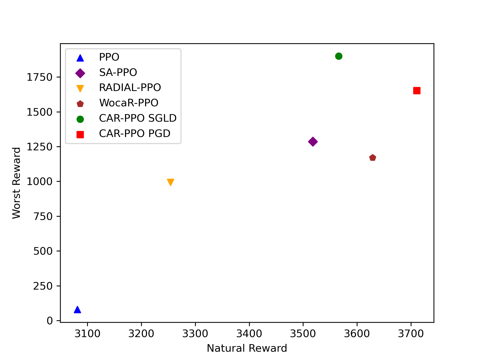
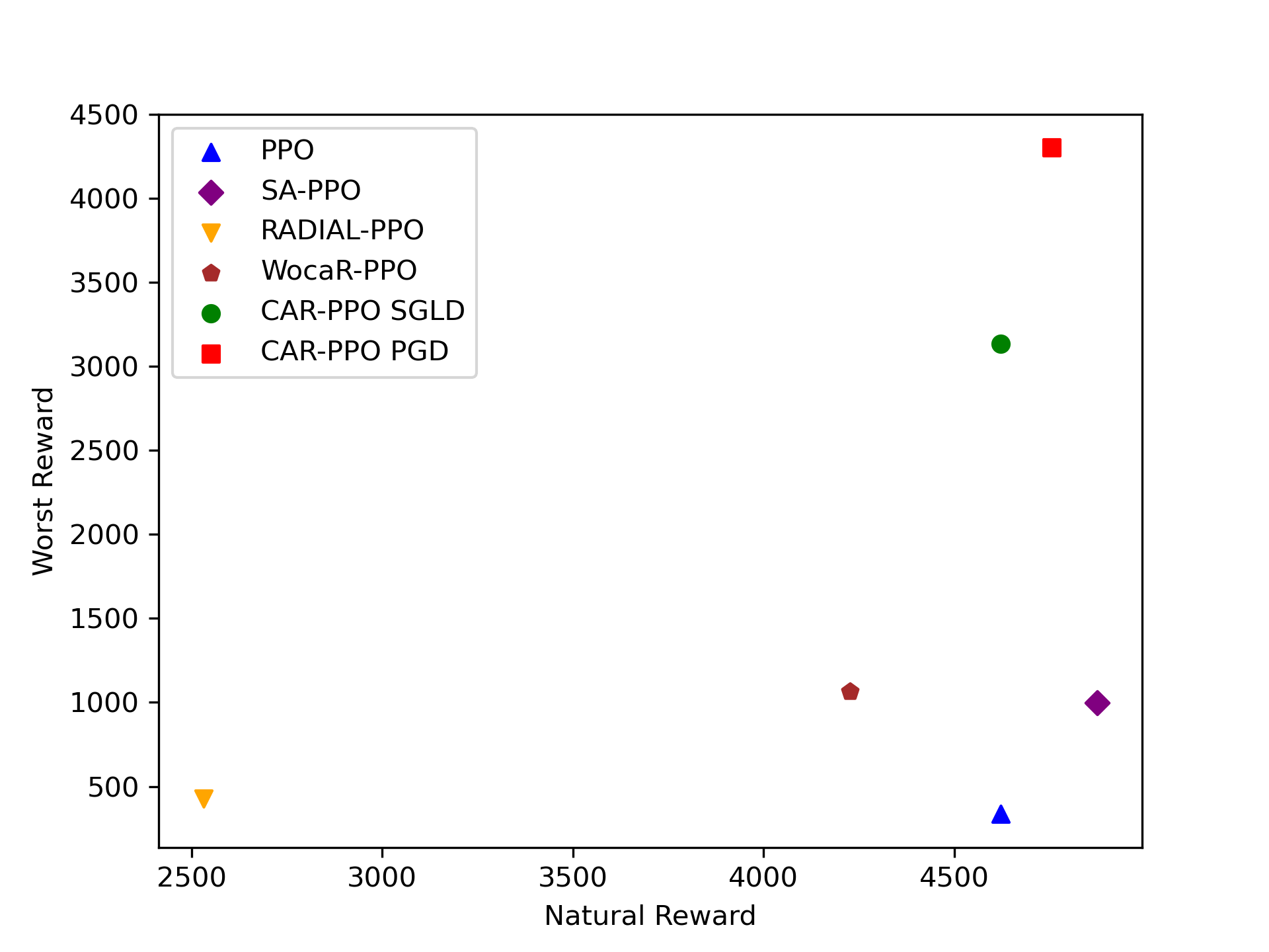
Hopper

Walker2d

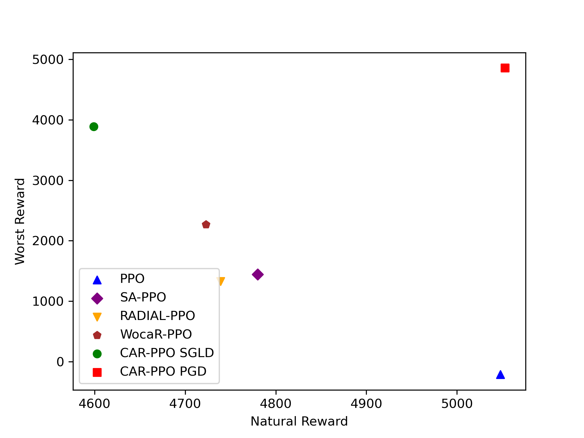
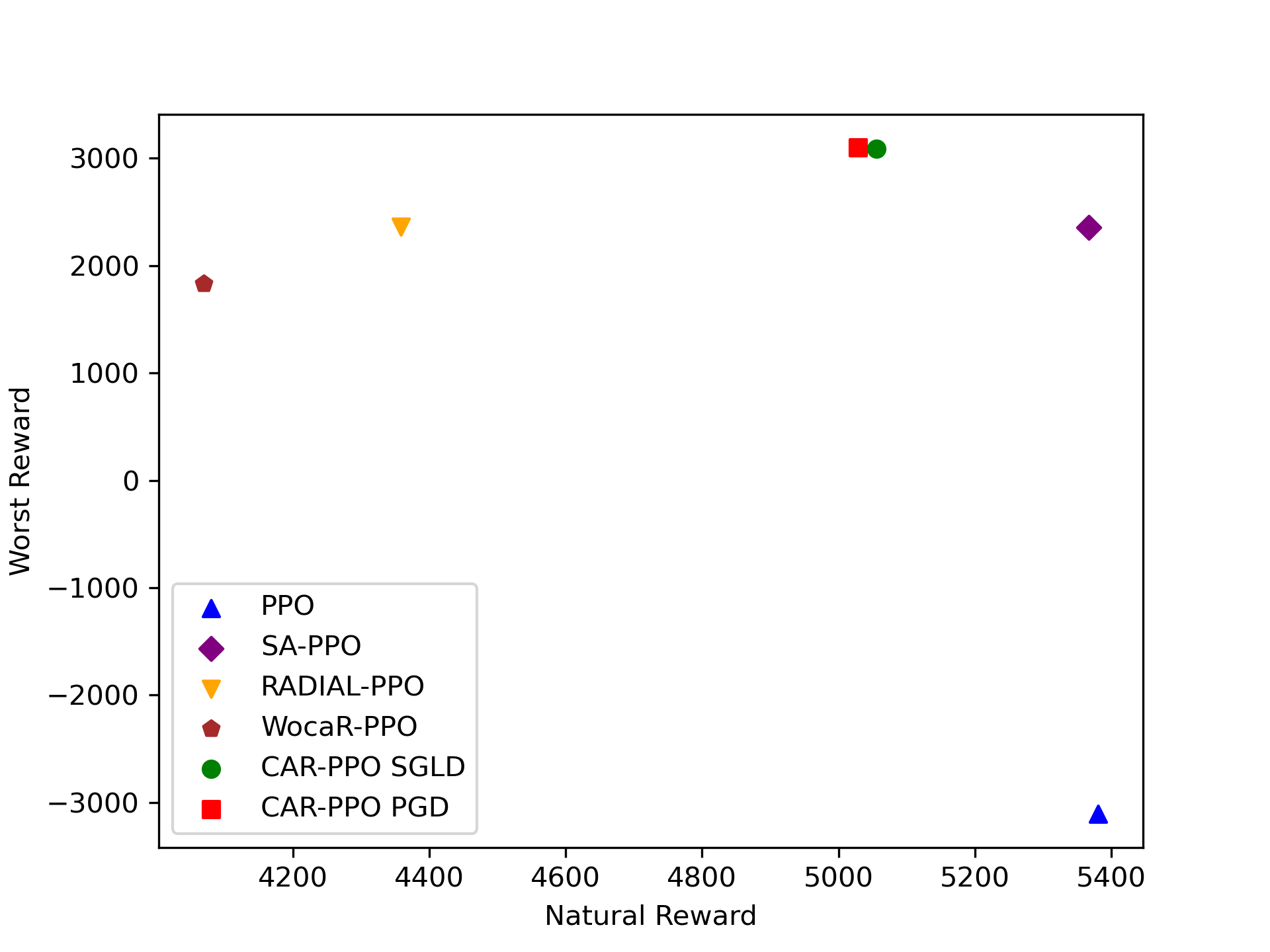
Halfcheetah

Ant

Figure 5: Natural reward and worst-case robustness under various attacks in MuJoCo.

CAR-DQN.

CAR-DQN is implemented based on Double Dueling DQN (Van Hasselt et al., 2016; Wang et al., 2016), and all baselines and CAR-DQN are trained for 4.5 million steps, based on the same standard model released by Zhang et al. (2020b), which has been trained for 6 million steps. We increase the attack $\epsilon$ from $0$ to $1/255$ during the first 4 million steps, using the same smoothed schedule as in Zhang et al. (2020b); Oikarinen et al. (2021); Liang et al. (2022), and then continue training with a fixed $\epsilon$ for the remaining 0.5 million steps. We use Huber loss to replace the absolute value function and separately apply classic gradient-based methods (PGD) and cheap convex relaxation (IBP) for resolving the inner optimization in $\mathcal{L}_{car}^{soft}(\theta)$. For CAR-DQN with the PGD solver, hyperparameters are the same as those of SA-DQN (Zhang et al., 2020b). For CAR-DQN with the IBP solver, we update the target network every 2000 steps, set the learning rate to $1.25\times 10^{-4}$, use a batch size of $32$, and set the exploration $\epsilon_{exp}$-end to $0.01$, soft coefficient $\lambda=1.0$ and discount factor to $0.99$. The replay buffer has a capacity of $2\times 10^{5}$, and we use the Adam optimizer (Kingma and Ba, 2015) with $\beta_{1}=0.9$ and $\beta_{2}=0.999$. The overall CAR-DQN algorithm process and additional details are shown in Appendix G.

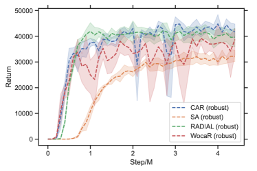
RoadRunner

BankHeist

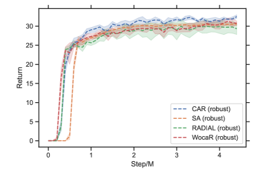
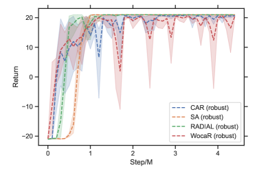
Freeway

Pong

Figure 6: Robust episode rewards of baselines and CAR-DQN under strong PGD attacks on 4 Atari games. Shaded regions are computed over 5 random seeds. CAR-DQN demonstrates superior robust performance in all environments.

CAR-PPO.

SA-PPO, WocaR-PPO, and CAR-PPO are trained for 2 million steps (976 iterations) on Hopper, Walker2d, and Halfcheetah, and 10 million steps (4882 iterations) on Ant for convergence. RADIAL-PPO are trained for 4 million steps (2000 iterations) on Hopper, Walker2d, and Halfcheetah following the official implementation and 10 million steps (4882 iterations) on Ant. We run 2048 simulation steps per iteration and use a simple MLP network for all PPO agents. The attack budget $\epsilon$ is linearly increased from $0$ to the target value during the first 732 iterations on Hopper, Walker2d, and Halfcheetah, and 3662 iterations on Ant, before continuing with the target value for the remaining iterations. This scheduler is aligned with Zhang et al. (2020b); Liang et al. (2022). We combine vanilla PPO with CAR loss for efficient training, using a regularization weight $\kappa$. The weight $\kappa$ is chosen from $\{0.1,0.3,1.0\}$. The soft coefficient $\lambda$ in $\mathcal{L}_{car}^{soft}(\theta)$ is chosen from $\{10,100,1000\}$ on Hopper, Walker2d and Halfcheetah and $\{100,1000,10000\}$ on Ant to ensure stable training. We separately apply PGD and SGLD (Gelfand and Mitter, 1991) to resolve the inner optimization in $\mathcal{L}_{car}^{soft}(\theta)$. We run 10 iterations with step size $\epsilon/10$ for both methods and set the temperature parameter $\beta=1\times 10^{-5}$ for SGLD. The overall CAR-PPO algorithm process and additional implementation details are shown in Appendix G.

7.2 Comparison Results

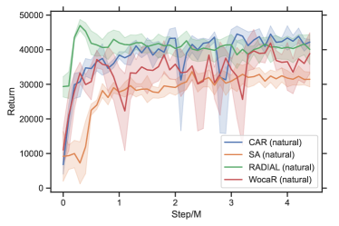
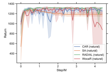
RoadRunner

BankHeist

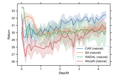
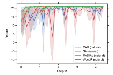
Freeway

Pong

Figure 7: Natural episode rewards of baselines and CAR-DQN without attacks on 4 Atari games. Shaded regions are computed over 5 random seeds. CAR-DQN demonstrates superior natural performance in all environments.

Evaluation on Atari.

Table 1 presents the natural and robust performance of DQN agents, all of which are trained using a perturbation radius of $\epsilon=1/255$ and evaluated under attacks with $\epsilon=1/255,\ 3/255,\ 5/255$. For the $\epsilon=1/255$ attacks, it is worth noting that CAR-DQN agents exhibit superior performance compared to baselines in the most challenging RoadRunner environment, achieving significant improvements in both natural and robust rewards. In the other three games, CAR-DQN matches the performance of the state-of-the-art baseline well. Our CAR-DQN loss function coupled with the PGD solver, achieves an impressive return of around 45,000 on the RoadRunner environment, significantly surpassing SA-DQN with the PGD approach. It also attains $60\%$ higher robust rewards under the MinBest attack on the Freeway game. For attacks with increasing perturbation radius $\epsilon=3/255,\ 5/255$, We can see that CAR-DQN agents achieve superior performance in Pong and BankHeist, and attain comparable performance in Freeway. Notably, in more complex environments like BankHeist and RoadRunner, SA-DQN with the PGD solver fails to maintain robustness under larger perturbations. In contrast, CAR-DQN with the PGD solver, trained under the small perturbation budget, maintains strong robust performance even with larger attack budgets. In addition, we also notice that RADIAL-DQN outperforms CAR-DQN under large perturbation budgets on RoadRunner, for which extensive analysis and comparisons are provided in Appendix H.2. We also compare the two solvers and find that PGD shows weaker robustness than convex relaxation, particularly failing to ensure the ACR computed with relaxation bounds. This discrepancy can be attributed to that the PGD solver offers a lower bound surrogate function of the loss, while the IBP solver provides an upper bound.

Evaluation on MuJoCo.

Table 2 showcases the natural and robust performance of CAR-PPO and baselines. Hopper agents are trained and attacked with a perturbation radius of $\epsilon=0.075$, Walker2d agents are with $\epsilon=0.05$, and Halfcheetah and Ant agents are with $\epsilon=0.15$. Notably, CAR-PPO agents achieve the best robustness in the worst case across all four environments, with significant 55%, 304%, 114%, 31% improvement on Hopper, Walker2d, Halfcheetah, and Ant, respectively. Meanwhile, the natural performance of CAR-PPO agents also matches the best level in each environment. CAR-PPO agents with the PGD solver achieve the highest natural performance on Hopper and Halfcheetah, outperform vanilla PPO agents on Walker2d, and attain comparable natural rewards on Ant. While CAR-PPO is slightly $2.5\%,\ 6.3\%$ lower in natural performance than SA-PPO on Walker2d and Ant, it respectively achieves $332\%$ and $32\%$ higher worst-case robustness. The overall performance of CAR-PPO with PGD is better than CAR-PPO with SGLD, underscoring the importance of the PGD method for training robust PPO agents. More intuitive comparisons of natural and worst-case robust performance are shown in Fig. 5.

Table 3: Performance of DQN with different Bellman $p$-error.

Environment	Norm	Natural	PGD	MinBest	ACR
Pong	$L^{1}$	$\bf 21.0\pm 0.0$	$-21.0\pm 0.0$	$-21.0\pm 0.0$	$0$
	$L^{2}$	$\bf 21.0\pm 0.0$	$-21.0\pm 0.0$	$-20.8\pm 0.1$	$0$
	$L^{\infty}$	$\bf 21.0\pm 0.0$	$\bf 21.0\pm 0.0$	$\bf 21.0\pm 0.0$	$0.985$
Freeway	$L^{1}$	$\bf 33.9\pm 0.1$	$0.0\pm 0.0$	$0.0\pm 0.0$	$0$
	$L^{2}$	$21.8\pm 0.3$	$21.7\pm 0.3$	$22.1\pm 0.3$	$0$
	$L^{\infty}$	$33.3\pm 0.1$	$\bf 33.2\pm 0.1$	$\bf 33.2\pm 0.1$	$0.981$
BankHeist	$L^{1}$	$1325.5\pm 5.7$	$27.0\pm 2.0$	$0.0\pm 0.0$	$0$
	$L^{2}$	$1314.5\pm 4.0$	$18.5\pm 1.5$	$22.5\pm 2.6$	$0$
	$L^{\infty}$	$\bf 1356.0\pm 1.7$	$\bf 1356.5\pm 1.1$	$\bf 1356.5\pm 1.1$	$0.969$
RoadRunner	$L^{1}$	$43795\pm 1066$	$0\pm 0$	$0\pm 0$	$0$
	$L^{2}$	$30620\pm 990$	$0\pm 0$	$0\pm 0$	$0$
	$L^{\infty}$	$\bf 49500\pm 2106$	$\bf 48230\pm 1648$	$\bf 48050\pm 1642$	$0.947$

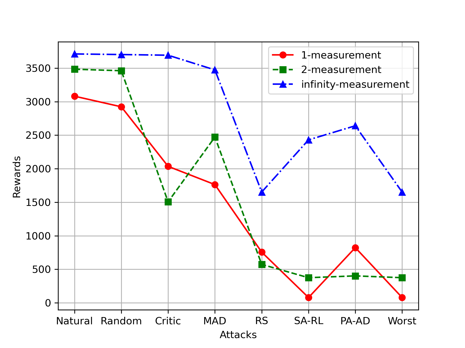
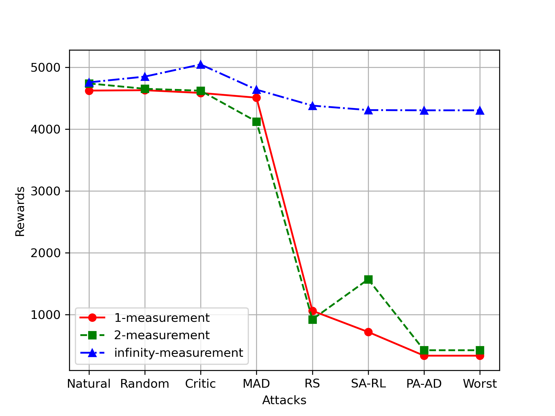
Hopper

Walker2d

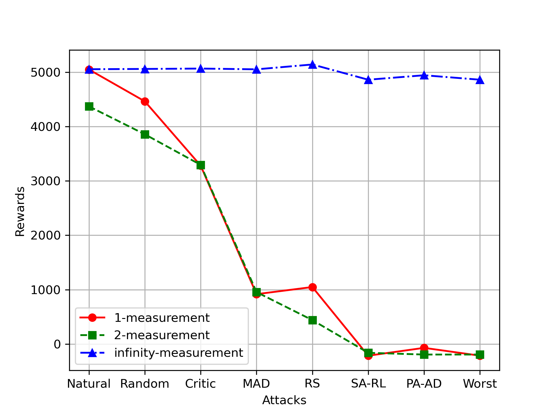
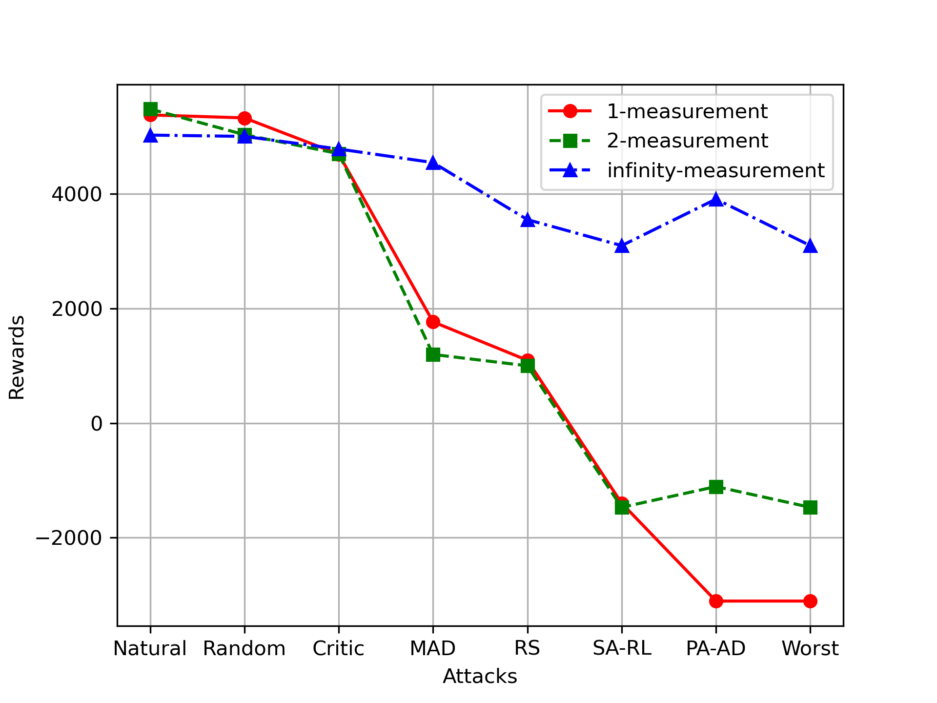
Halfcheetah

Ant

Figure 8: Performance of PPO with different $k$-measurement errors.

Consistency in Natural and PGD Attack Returns on Atari.

Figure 2 records the natural and PGD attack returns of CAR-DQN agents during training, showcasing strong alignment between natural performance and robustness across all environments. This consistency supports our theory that the ORP is aligned with the Bellman optimal policy and confirms the rationality of the proposed ISA-MDP framework. Additionally, Figures 7 and 6 illustrate the natural episode returns and robustness during training for various algorithms. It is worth noting that CAR-DQN agents quickly and stably converge to peak robustness and natural performance across all environments, while other algorithms exhibit unstable trends. For instance, the natural reward curves of SA-DQN and WocaR-DQN on BankHeist and RADIAL-DQN on RoadRunner show notable declines, and the robust curves of SA-DQN and WocaR-DQN on BankHeist also tend to decrease. These discrepancies primarily arise from their robustness objectives that deviate from the standard training loss, leading to learning sub-optimal actions. In contrast, the consistent objective of CAR-DQN ensures that it always learns optimal actions in both natural and robust contexts.

Training Efficiency.

Training times for SA-DQN, RADIAL-DQN, WocaR-DQN, and CAR-DQN are approximately 27, 12, 20, and 14 hours, respectively, all trained for 4.5 million frames on identical hardware with a GeForce RTX 3090 GPU. All robust PPO agents require around 2 hours to train on Hopper, Walker2d, and Halfcheetah, and 9 hours on Ant, on the same device with an AMD EPYC 7742 CPU. Additionally, our CAR loss incurs no additional memory consumption compared to vanilla training.

7.3 Ablation Studies

Necessity of Infinity Measurement Errors.

To verify the necessity of the $(\infty,d_{\mu_{0}}^{\pi})$-norm in action-value function spaces for adversarial robustness, we train DQN agents using the Bellman error under the $(1,d_{\mu_{0}}^{\pi})$-norm and $(2,d_{\mu_{0}}^{\pi})$-norm, respectively. We then compare their performance with our CAR-DQN, which approximates the Bellman error under the $(\infty,d_{\mu_{0}}^{\pi})$-norm. All agents are trained and evaluated with a perturbation budget $\epsilon=1/255$. As shown in Table 3, all agents perform well without attacks across the four games. However, agents using the $(1,d_{\mu_{0}}^{\pi})$-norm and $(2,d_{\mu_{0}}^{\pi})$-norm experience significant performance degradation under strong attacks, with episode rewards dropping near the lowest values for each game. These results are highly consistent with Theorem 10, confirming the importance of the $(\infty,d_{\mu_{0}}^{\pi})$-norm for robust performance.

To validate the necessity of infinity measurement errors in probability spaces, we train PPO agents that rely on $1$-measurement and $2$-measurement errors, respectively. We then compare their performance to our CAR-PPO agents, which are trained with surrogates of infinity measurement errors. As depicted in Figure 8 and Table 8, all agents achieve good performance in natural environments and under weak attacks across the four continuous control tasks. However, agents trained with $1$-measurement and $2$-measurement errors exhibit similar and quite poor performance in environments with strong attacks. In contrast, agents using infinity measurement errors maintain strong robustness across all tasks. These experimental phenomenons align with Theorems 20 and 21, underscoring the critical role of infinity measurement errors for robust DRL agents.

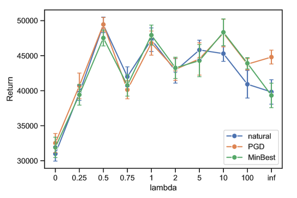
Figure 9: Natural, PGD attack, and MinBest attack rewards of CAR-DQN with different soft coefficients $\lambda$ on the RoadRunner game.

Table 4: Ablation studies for soft coefficients on 4 Atari games.

Environment	$\lambda$	Natural	PGD	MinBest	ACR
Pong	$0$	$\bf 21.0\pm 0.0$	$\bf 21.0\pm 0.0$	$\bf 21.0\pm 0.0$	$0.972$
	$1$	$\bf 21.0\pm 0.0$	$\bf 21.0\pm 0.0$	$\bf 21.0\pm 0.0$	$0.985$
	$\infty$	$20.6\pm 0.1$	$20.7\pm 0.1$	$20.7\pm 0.1$	$0.980$
Freeway	$0$	$31.6\pm 0.2$	$31.5\pm 0.1$	$31.5\pm 0.1$	$0.966$
	$1$	$\bf 33.3\pm 0.1$	$\bf 33.2\pm 0.1$	$\bf 33.2\pm 0.1$	$0.981$
	$\infty$	$31.5\pm 0.1$	$30.9\pm 0.3$	$31.2\pm 0.2$	$0.967$
BankHeist	$0$	$1307.5\pm 11.0$	$1288.5\pm 14.0$	$1284.0\pm 13.8$	$0.980$
	$1$	$\bf 1356.0\pm 1.7$	$\bf 1356.5\pm 1.1$	$\bf 1356.5\pm 1.1$	$0.969$
	$\infty$	$1326.0\pm 4.8$	$1316.0\pm 6.8$	$1314.0\pm 6.6$	$0.979$
RoadRunner	$0$	$25160\pm 802$	$24540\pm 760$	$26785\pm 617$	$0.007$
	$1$	$\bf 49500\pm 2106$	$\bf 48230\pm 1648$	$\bf 48050\pm 1642$	$0.947$
	$\infty$	$40890\pm 2075$	$36760\pm 1874$	$36740\pm 2098$	$0.940$

Effects of Soft Coefficient $\lambda$.

We assess the impact of the soft coefficient $\lambda$ on the CAR-DQN loss function by training agents in the RoadRunner environment with varying values of $\lambda$ ranging from $0$ to $\infty$, validating the effectiveness of soft CAR loss. When $\lambda=0$, the agent utilizes only the sample with the largest adversarial TD-error within the batch, whereas $\lambda=\infty$ corresponds to averaging over all samples in the batch. It is important to note that small values of $\lambda$ can lead to numerical instability. As depicted in Figure 9, agents exhibit similar capabilities when $0.5\leq\lambda\leq 10$, indicating that the learned policies are relatively insensitive to the soft coefficient within this range. Table 4 presents the performance of CAR-DQN agents with $\lambda=0,1,\infty$ across four Atari environments. In the RoadRunner, $\lambda=0$ results in poor performance, achieving returns of around 25,000 due to insufficient utilization of the samples. Interestingly, utilizing only the sample with the largest adversarial TD error in the batch achieves good robustness in the other three simpler games. The case $\lambda=\infty$ results in weaker robustness compared to other cases with differentiated weights. This suggests that each sample in the batch plays a distinct role in robust training, and assigning appropriate weights to the samples in a batch enhances robust performance. These results further validate the efficacy of our CAR-DQN loss function.

Additionally, we evaluate the effects of the soft coefficient $\lambda$ through training CAR-PPO with various solvers and soft coefficients. As shown in Table 5, in Hopper and Ant tasks, CAR-PPO agents show similar performance under selected coefficients and solvers, indicating that trained policies are relatively insensitive to the soft coefficient under these settings. In Walker2d and Halfcheetah environments, CAR-PPO agents are more sensitive to different $\lambda$, further confirming the effectiveness of the CAR-PPO loss function.

Table 5: Ablation studies for soft coefficients on 4 Mujoco tasks.

Env	Solver	$\lambda$	Natural Reward	Attack Reward
				Random	Critic	MAD	RS	SA-RL	PA-AD	Worst
Hopper ($\epsilon$=0.075)	SGLD ($\kappa$=1.0)	10	3148	3090	3552	3211	2292	1554	2492	1554
		100	3566	3537	3480	3484	1990	2977	3232	1990
		1000	3540	3487	3622	3324	1079	1079	2133	1079
	PGD ($\kappa$=0.3)	10	3660	3604	3283	3046	1426	601	2444	601
		100	3608	3734	3745	2946	1610	1103	1888	1103
		1000	3711	3702	3692	3473	1652	2430	2640	1652
Walker2d ($\epsilon$=0.05)	SGLD ($\kappa$=0.1)	10	4622	4609	4684	4498	4242	4397	3134	3134
		100	3649	3252	3947	3607	1979	650	689	650
		1000	4323	4326	4308	4340	4323	4137	2073	2073
	PGD ($\kappa$=1.0)	10	3247	3262	3771	3216	1449	1098	1416	1098
		100	4755	4848	5045	4637	4379	4308	4303	4303
		1000	3400	3296	3136	3469	2937	1516	1362	1362
Halfcheetah ($\epsilon$=0.15)	SGLD ($\kappa$=0.1)	10	3953	3967	3862	4008	3792	3273	3334	3273
		100	5131	5059	4803	3131	3360	3032	1507	1507
		1000	4599	4574	4731	4348	3888	3908	4032	3888
	PGD ($\kappa$=1.0)	10	4751	4741	4676	4712	4354	4389	4501	4354
		100	3291	3298	3528	3341	3126	2991	3159	2991
		1000	5053	5058	5065	5053	5140	4860	4942	4860
Ant ($\epsilon$=0.15)	SGLD ($\kappa$=0.1)	100	5056	5007	4864	4468	3755	3088	3763	3088
		1000	5283	5180	4798	4469	3292	2387	3442	2387
		10000	5187	5008	4997	4589	3715	2322	3527	2322
	PGD ($\kappa$=0.3)	100	4901	4807	4401	4429	3876	3197	3917	3197
		1000	5074	4937	4838	4536	2779	2961	3889	2776
		10000	5029	5006	4787	4549	3553	3099	3911	3099

8 Conclusion and Future Work

In this paper, we demonstrate the alignment of the optimal robust policy with the Bellman optimal policy within the universal Intrinsic State-adversarial MDP framework. We prove that optimizing different $k$-measurement errors yields varied performance, underscoring the necessity of infinity measurement errors for achieving adversarial robustness. Our findings are validated through experiments with CAR-DQN and CAR-PPO, which optimize surrogate objectives of infinity measurement errors. We believe this work contributes significantly to unveiling the nature of adversarial robustness in reinforcement learning.

Our theoretical focus primarily addresses the necessity of infinity measurements in the worst-case scenario. In future work, we plan to explore how DRL agents converge to vulnerable models from the perspective of feature learning theory. Additionally, the CAR operator we introduced to characterize the adversarial robust training involves a bilevel optimization problem, and robust training itself can be framed as a minimax problem. We aim to investigate these aspects further, leveraging bilevel and minimax optimization theories and techniques to improve the efficiency of robust training.

Appendix A Examples of Intrinsic States

In Figure 10, 11, 12, we show some examples in 3 Atari games (Pong, Freeway, and RoadRunner), indicating that the state observation $s$ and adversarial observation $s_{\nu}$ share the same intrinsic state.

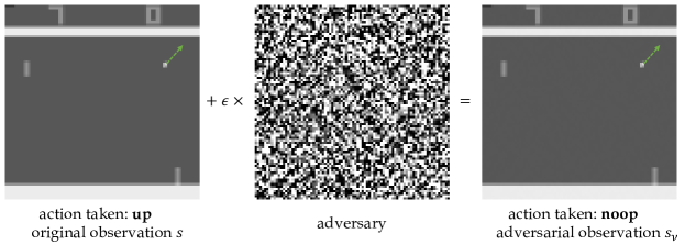
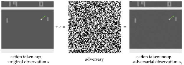
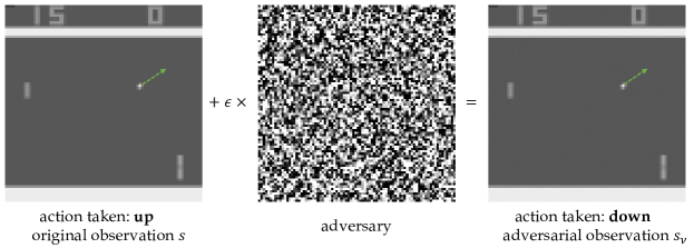
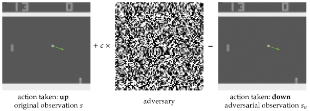
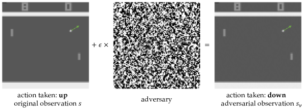
Figure 10: Examples of intrinsic states in Pong games. The direction for the movement of the ball is marked.

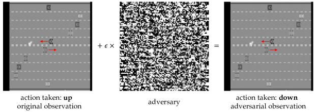
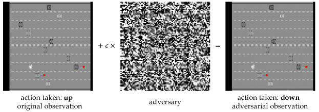
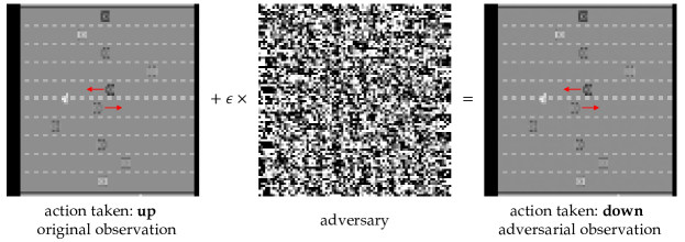
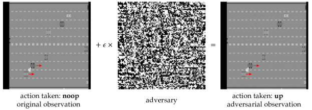
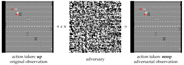
Figure 11: Examples of intrinsic states in Freeway games. The directions for the movement of cars around the chicken are marked.

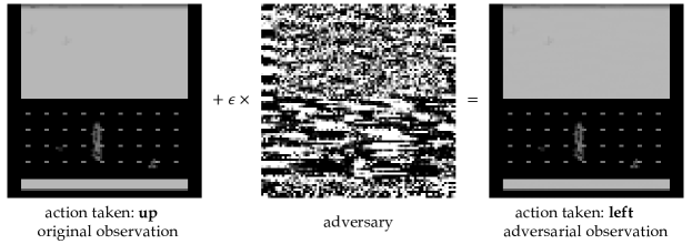
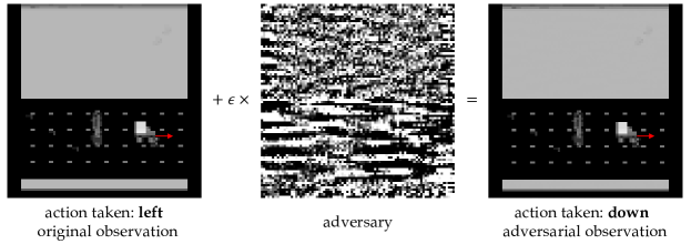
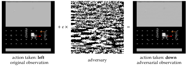
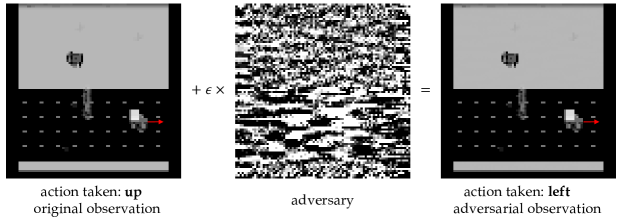
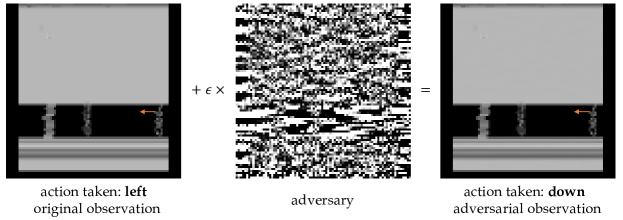
Figure 12: Examples of intrinsic states in RoadRunner games. The directions for the movement of trucks and competitors are marked.

Appendix B Theorems and Proofs of Optimal Adversarial Robustness

B.1 Characterization of the Sparse Difference Between Intrinsic and Standard State Neighborhoods

Theorem 23

For any MDP $\mathcal{M}$, let $\mathcal{S}_{nu}$ denote the state set where the optimal action is not unique, i.e. $\mathcal{S}_{nu}=\left\{s\in\mathcal{S}|\mathop{\arg\max}_{a}Q^{*}(s,a)\text{ is not a singleton}\right\}$. Then we have the following conclusions:

• Let $\mathcal{S}^{\prime}=\{s\in S|\exists\ a\in A,\text{s.t. }Q^{*}(s,a)\ \text{is not continuous at}\ s\}$, then for all $s\in\left(\mathcal{S}\setminus\mathcal{S}_{nu}\right)\setminus\mathcal{S}^{\prime}$, there exists $\epsilon>0$ such that $B_{\epsilon}(s)=B^{*}_{\epsilon}(s)$.

• Given $\epsilon>0$, let $\mathcal{S}_{nin}$ denote the set of states where the intrinsic state $\epsilon$-neighourhood is not the same as the $\epsilon$-neighourhood, i.e. $\mathcal{S}_{nin}=\left\{s\in\mathcal{S}|B_{\epsilon}(s)\neq B^{*}_{\epsilon}(s)\right\}$. Then, we have $\mathcal{S}_{nin}\subseteq\mathcal{S}_{nu}\cup\mathcal{S}_{0}+B_{\epsilon}$, where $\mathcal{S}_{0}$ is the set of discontinuous points that cause the optimal action to change, i.e. $\mathcal{S}_{0}=\{s\in S|\forall\ \epsilon_{1}>0,\exists\ s^{\prime}\in B_{\epsilon_{1}}(s),\text{s.t. }\arg\max_{a}Q^{*}(s^{\prime},a)\neq\arg\max_{a}Q^{*}(s,a)\}\cap\mathcal{S}^{\prime}$.

Proof  (1) Let $\mathcal{S}^{\prime}=\{s\in\mathcal{S}|\exists a\in\mathcal{A},\text{s.t. $Q^{*}(s,a)$ is not continuous at }s\}$, then we have that $Q^{*}(s,a)$ is continuous in $\mathcal{S}\setminus\left(\mathcal{S}_{nu}\cup\mathcal{S}^{\prime}\right)$.

Because $\arg\max_{a}Q^{*}(s,a)$ is a singleton for $\mathcal{S}\setminus\left(\mathcal{S}_{nu}\cup\mathcal{S}^{\prime}\right)$, we can define $\arg\max_{a}Q^{*}(s,a)=\{a_{s}^{*}\}$ for any $s\in\left(\mathcal{S}\setminus\mathcal{S}_{nu}\right)\setminus\mathcal{S}^{\prime}$. Then, we have that

$$Q^{*}(s,a_{s}^{*})>Q^{*}(s,a)\text{ for a fixed }a\in\mathcal{A}\setminus\{a_{s}^{*}\}.$$

According to continuity of $Q^{*}(\cdot,a)$ for all $a\in\mathcal{A}$, there exists $\epsilon_{a}>0$, such that

$$Q^{*}(s^{\prime},a_{s}^{*})>Q^{*}(s^{\prime},a)\text{ for all }s^{\prime}\in B_{\epsilon_{a}}(s).$$

Because $\mathcal{A}$ is a finite discrete set, let $\epsilon=\min_{a\in\mathcal{A}\setminus{a_{s}^{*}}}\{\epsilon_{a}\}$, then we have that

$$Q^{*}(s^{\prime},a_{s^{\prime}}^{*})>Q^{*}(s^{\prime},a)\qquad\forall s^{\prime}\in B_{\epsilon}(s)\text{ and }a\in\mathcal{A}\setminus\{a_{s^{\prime}}^{*}\},$$

which indicates that we have

$$B_{\epsilon}(s)=B_{\epsilon}^{*}(s).$$

(2) Let $\mathcal{S}_{n}=\{s\in\mathcal{S}|\forall\epsilon_{1}>0,\exists s^{\prime}\in B_{\epsilon_{1}}(s),\ \text{s.t. }\arg\max_{a}Q^{*}(s^{\prime},a)\neq\arg\max_{a}Q^{*}(s,a)\}$ and $\mathcal{S}_{0}=\mathcal{S}_{n}\cap\mathcal{S}^{\prime}$. Then $S_{0}$ is the set of discontinuous points that cause the optimal action to change. And $\mu(\mathcal{S}_{0})=\mu(\mathcal{S}_{n}\cap\mathcal{S}^{\prime})=0$ because $\mu(\mathcal{S}^{\prime})=0$.

For any $s\in\mathcal{S}_{nin}=\left\{s\in\mathcal{S}|B_{\epsilon}(s)\neq B^{*}_{\epsilon}(s)\right\}$, we have the following two cases.

Case 1. $\exists s^{\prime}\in B_{\epsilon}(s)$ s.t. $s^{\prime}\in\mathcal{S}_{nu}$, then $s\in\mathcal{S}_{nu}+B_{\epsilon}$, i.e.

$$s\in\mathcal{S}_{nu}\cup\mathcal{S}_{0}+B_{\epsilon}.$$

Case 2. $\forall s^{\prime}\in B_{\epsilon}(s),s^{\prime}\notin\mathcal{S}_{nu}$, which means that $\arg\max_{a}Q^{*}(s^{\prime},a)$ is a singleton for all $s^{\prime}\in B_{\epsilon}(s)$. Define $\arg\max_{a}Q^{*}(s^{\prime},a)=\{a_{s^{\prime}}^{*}\}$ for any $s^{\prime}\in B_{\epsilon}(s)$.

Because $s\in\mathcal{S}_{nin}$, there exist a $s^{\prime}\in B_{\epsilon}(s)$ such that $a_{s^{\prime}}^{*}\neq a_{s}^{*}$. Let $s_{1}$ be the point that closest to $s$ satisfing $a_{s_{1}}^{*}\neq a_{s}^{*}$, then $s_{1}\in B_{\epsilon}(s)$. We have

$$s_{1}\in\mathcal{S}_{n}.$$ (1)

Otherwise $s_{1}\notin\mathcal{S}_{n}$ means that $\exists\epsilon_{1}>0,\forall s^{\prime}\in B_{\epsilon_{1}}(s_{1})$, $a_{s^{\prime}}^{*}=a_{s_{1}}^{*}$, then $s_{1}$ is not the point that closest to $s$ satisfing $a_{s_{1}}^{*}\neq a_{s}^{*}$, which is a contradiction. We also have

$$s_{1}\in\mathcal{S}^{\prime}.$$ (2)

Otherwise $s_{1}\notin\mathcal{S}^{\prime}$ means that $\forall a\in\mathcal{A}$, $Q^{*}(\cdot,a)$ is continuous in $s_{1}$. First, we have

$$Q^{*}(s_{1},a_{s_{1}}^{*})>Q^{*}(s_{1},a),\forall a\in\mathcal{A}\setminus\{a_{s_{1}}^{*}\}.$$

Then $\exists\ \epsilon_{2}>0$, $\forall s\in B_{\epsilon_{2}}(s_{1})$, s.t.

$$Q^{*}(s,a_{s_{1}}^{*})>Q^{*}(s,a),\forall a\in\mathcal{A}\setminus\{a_{s_{1}}^{*}\}.$$

because of the continuity of point $s_{1}$. This contradicts the definition of $s_{1}$.

According to (1) and (2), we have $s_{1}\in\mathcal{S}^{\prime}\cap\mathcal{S}_{n}$ i.e. $s_{1}\in\mathcal{S}_{0}$. Then $s\in\mathcal{S}_{0}+B_{\epsilon}(s)$, i.e.

$$s\in\mathcal{S}_{nu}\cup\mathcal{S}_{0}+B_{\epsilon}.$$

Thus

$$\mathcal{S}_{nin}\subseteq\mathcal{S}_{nu}\cup\mathcal{S}_{0}+B_{\epsilon}.$$

Therefore, the proof of the theorem is concluded.  

Remark 24

In practical complex tasks, we can view $\mathcal{S}_{nu}$ as an empty set.

Remark 25

Except for the smooth environment, many tasks can be modeled as environments with sparse rewards. Further, the value and action-value functions in these environments are almost everywhere continuous, indicating the set $\mathcal{S}_{0}$ is a zero-measure set.

Remark 26

According to the above characteristics, we know that $\mathcal{S}_{0}$ is a set of special discontinuous points and its elements are rare in practical complex environments.

Further, we can get the following corollary in the setting of continuous functions and there are better conclusions.

Corollary 27

For any MDP $\mathcal{M}$, let $\mathcal{S}_{nu}$ denote the state set where the optimal action is not unique, i.e. $\mathcal{S}_{nu}=\left\{s\in\mathcal{S}|\mathop{\arg\max}_{a}Q^{*}(s,a)\text{ is not a singleton}\right\}$. If $Q^{*}(\cdot,a)$ is continuous in $\mathcal{S}$ for all $a\in\mathcal{A}$, we have the following conclusions:

• For $s\in\mathcal{S}\setminus\mathcal{S}_{nu}$, there exists $\epsilon>0$ such that $B_{\epsilon}(s)=B^{*}_{\epsilon}(s)$.

• Given $\epsilon>0$, let $\mathcal{S}_{nin}$ denote the set of states where the intrinsic state $\epsilon$-neighourhood is not the same as the $\epsilon$-neighourhood, i.e. $\mathcal{S}_{nin}=\left\{s\in\mathcal{S}|B_{\epsilon}(s)\neq B^{*}_{\epsilon}(s)\right\}$. Then, we have $\mathcal{S}_{nin}\subseteq\mathcal{S}_{nu}+B_{\epsilon}=\left\{s_{1}+s_{2}|s_{1}\in\mathcal{S}_{nu},\ \|s_{2}\|\leq\epsilon\right\}$. Especially, when $\mathcal{S}_{nu}$ is a finite set, we have $\mu\left(\mathcal{S}_{nin}\right)\leq\left|\mathcal{S}_{nu}\right|\mu\left(B_{\epsilon}\right)=C_{d}\left|\mathcal{S}_{nu}\right|\epsilon^{d}$, where $C_{d}$ is a constant with respect to dimension $d$ and norm.

Proof  Corollary 27 can be derived from Theorem 23 because we have the following conclusion in continuous case.

$$\mathcal{S}_{0}\subseteq\{s\in\mathcal{S}|\exists a\in\mathcal{A},\text{s.t. $Q^{*}(s,a)$ is not continuous at }s\}=\emptyset.$$

Therefore, the theorem is concluded.  

Remark 28

Certain natural environments show smooth reward function and transition dynamics, especially in continuous control tasks where the transition dynamics come from some physical laws. Further, the value and action-value functions in these environments are continuous, making $\mathcal{S}_{0}$ an empty set.

B.2 Consistent Optimal Robust Policy and CAR Operator

Define the consistent adversarial robust operator for adversarial action-value function:

$$\left(\mathcal{T}_{car}Q\right)(s,a)=r(s,a)+\gamma\mathbb{E}_{s^{\prime}\sim\mathbb{P}(\cdot|s,a)}\left[\min_{s^{\prime}_{\nu}\in B_{\epsilon}(s^{\prime})}Q\left(s^{\prime},\mathop{\arg\max}_{a_{s^{\prime}_{\nu}}}Q\left(s^{\prime}_{\nu},a_{s^{\prime}_{\nu}}\right)\right)\right].$$

B.2.1 CAR Operator is Not a Contraction

Theorem 29

$\mathcal{T}_{car}$ is not a contraction.

Proof  Let $\mathcal{S}=[-1,1]$, $\mathcal{A}=\{a_{1},a_{2}\}$, $0<\epsilon\ll 1$ and dynamic transition $\mathbb{P}(\cdot|s,a)$ be a determined function. Let $n>\max\{\frac{\delta}{\gamma},2\delta\}$, $\delta>0$ and

$$Q_{1}(s,a_{1}) =2n\cdot\mathbbm{1}_{\left\{s\in\left[-1,0\right)\right\}}+\left[2n-\frac{2n-2\delta}{\frac{1}{8}\epsilon}s\right]\cdot\mathbbm{1}_{\left\{s\in\left[0,\frac{1}{8}\epsilon\right)\right\}}+2\delta\cdot\mathbbm{1}_{\left\{s\in\left[\frac{1}{8}\epsilon,\frac{3}{8}\epsilon\right)\right\}}$$

$$+\left[2\delta+\frac{n-2\delta}{\frac{1}{8}\epsilon}\left(s-\frac{3\epsilon}{8}\right)\right]\cdot\mathbbm{1}_{\left\{s\in\left[\frac{3}{8}\epsilon,\frac{1}{2}\epsilon\right)\right\}}+n\cdot\mathbbm{1}_{\left\{s\in\left[\frac{1}{2}\epsilon,1\right]\right\}},$$

$$Q_{1}(s,a_{2}) =n\cdot\mathbbm{1}_{\left\{s\in\left[-1,0\right)\right\}}+\left[n-\frac{n-\delta}{\frac{1}{8}\epsilon}s\right]\cdot\mathbbm{1}_{\left\{s\in\left[0,\frac{1}{8}\epsilon\right)\right\}}+\delta\cdot\mathbbm{1}_{\left\{s\in\left[\frac{1}{8}\epsilon,\frac{3}{8}\epsilon\right)\right\}}$$

$$+\left[\delta+\frac{2n-\delta}{\frac{1}{8}\epsilon}\left(s-\frac{3\epsilon}{8}\right)\right]\cdot\mathbbm{1}_{\left\{s\in\left[\frac{3}{8}\epsilon,\frac{1}{2}\epsilon\right)\right\}}+2n\cdot\mathbbm{1}_{\left\{s\in\left[\frac{1}{2}\epsilon,1\right]\right\}},$$

$$Q_{2}(s,a_{1}) =2n\cdot\mathbbm{1}_{\left\{s\in\left[-1,0\right)\right\}}+\left[2n-\frac{2n-\delta}{\frac{1}{8}\epsilon}s\right]\cdot\mathbbm{1}_{\left\{s\in\left[0,\frac{1}{8}\epsilon\right)\right\}}+\delta\cdot\mathbbm{1}_{\left\{s\in\left[\frac{1}{8}\epsilon,\frac{3}{8}\epsilon\right)\right\}}$$

$$+\left[\delta+\frac{n-\delta}{\frac{1}{8}\epsilon}\left(s-\frac{3\epsilon}{8}\right)\right]\cdot\mathbbm{1}_{\left\{s\in\left[\frac{3}{8}\epsilon,\frac{1}{2}\epsilon\right)\right\}}+n\cdot\mathbbm{1}_{\left\{s\in\left[\frac{1}{2}\epsilon,1\right]\right\}},$$

$$Q_{2}(s,a_{2}) =n\cdot\mathbbm{1}_{\left\{s\in\left[-1,0\right)\right\}}+\left[n-\frac{n-2\delta}{\frac{1}{8}\epsilon}s\right]\cdot\mathbbm{1}_{\left\{s\in\left[0,\frac{1}{8}\epsilon\right)\right\}}+2\delta\cdot\mathbbm{1}_{\left\{s\in\left[\frac{1}{8}\epsilon,\frac{3}{8}\epsilon\right)\right\}}$$

$$+\left[2\delta+\frac{2n-2\delta}{\frac{1}{8}\epsilon}\left(s-\frac{3\epsilon}{8}\right)\right]\cdot\mathbbm{1}_{\left\{s\in\left[\frac{3}{8}\epsilon,\frac{1}{2}\epsilon\right)\right\}}+2n\cdot\mathbbm{1}_{\left\{s\in\left[\frac{1}{2}\epsilon,1\right]\right\}}.$$

Then

$$\|Q_{1}-Q_{2}\|_{L^{\infty}\left(\mathcal{S}\times\mathcal{A}\right)}=\delta.$$

We have

$$\mathcal{T}_{car}Q_{1}(s,a)-\mathcal{T}_{car}Q_{2}(s,a) =\gamma\mathbb{E}_{s^{\prime}\sim\mathbb{P}(\cdot|s,a)}\left[\min_{s^{1}_{\nu}\in B_{\epsilon}(s^{\prime})}Q_{1}\left(s^{\prime},\mathop{\arg\max}_{a_{s^{1}_{\nu}}}Q_{1}\left(s^{1}_{\nu},a_{s^{1}_{\nu}}\right)\right)-\right.$$

$$\left.\min_{s^{2}_{\nu}\in B_{\epsilon}(s^{\prime})}Q_{2}\left(s^{\prime},\mathop{\arg\max}_{a_{s^{2}_{\nu}}}Q_{2}\left(s^{2}_{\nu},a_{s^{2}_{\nu}}\right)\right)\right].$$

Let $\mathbb{P}(s^{\prime}=-\frac{\epsilon}{2}|s,a)=1$ and $s^{\prime}=-\frac{\epsilon}{2}$, then

$$\min_{s^{1}_{\nu}\in B_{\epsilon}(s^{\prime})}Q_{1}\left(s^{\prime},\mathop{\arg\max}_{a_{s^{1}_{\nu}}}Q_{1}\left(s^{1}_{\nu},a_{s^{1}_{\nu}}\right)\right)=Q_{1}(s^{\prime},a_{1}),$$

$$\min_{s^{1}_{\nu}\in B_{\epsilon}(s^{\prime})}Q_{2}\left(s^{\prime},\mathop{\arg\max}_{a_{s^{2}_{\nu}}}Q_{2}\left(s^{2}_{\nu},a_{s^{2}_{\nu}}\right)\right)=Q_{2}(s^{\prime},a_{2}).$$

Thus

$$\mathcal{T}_{car}Q_{1}(s,a)-\mathcal{T}_{car}Q_{2}(s,a)=\gamma\left[Q_{1}(s^{\prime},a_{1})-Q_{2}(s^{\prime},a_{2})\right]=\gamma n>\delta,$$

which means that

$$\|\mathcal{T}_{car}Q_{1}-\mathcal{T}_{car}Q_{2}\|_{L^{\infty}\left(\mathcal{S}\times\mathcal{A}\right)}>\|Q_{1}-Q_{2}\|_{L^{\infty}\left(\mathcal{S}\times\mathcal{A}\right)}.$$

Therefore, $\mathcal{T}_{car}$ is not a contraction.  

B.2.2 Fixed Point of CAR Operator

Lemma 30 (Bellman equations for fixed $\pi$ and $\nu$ in SA-MDP, Zhang et al. (2020b))

Given $\pi:\mathcal{S}\rightarrow\Delta(\mathcal{A})$ and $\nu:\mathcal{S}\rightarrow\mathcal{S}$, we have

$$V^{\pi\circ\nu}(s) =\mathbb{E}_{a\sim\pi\left(\cdot|{\nu\left(s\right)}\right)}Q^{\pi\circ\nu}(s,a)$$

$$=\mathbb{E}_{a\sim\pi\left(\cdot|{\nu\left(s\right)}\right)}\left[r(s,a)+\gamma\mathbb{E}_{s^{\prime}\sim\mathbb{P}(\cdot|s,a)}V^{\pi\circ\nu}(s^{\prime})\right],$$

$$Q^{\pi\circ\nu}(s,a) =r(s,a)+\gamma\mathbb{E}_{s^{\prime}\sim\mathbb{P}(\cdot|s,a)}V^{\pi\circ\nu}(s^{\prime})$$

$$=r(s,a)+\gamma\mathbb{E}_{s^{\prime}\sim\mathbb{P}(\cdot|s,a),a^{\prime}\sim\pi\left(\cdot|{\nu\left(s^{\prime}\right)}\right)}Q^{\pi\circ\nu}(s^{\prime},a^{\prime}).$$

Lemma 31 (Bellman equation for strongest adversary $\nu^{*}$ in SA-MDP, Zhang et al. (2020b))

$$V^{\pi\circ\nu^{*}(\pi)}(s)=\min_{\nu(s)\in B(s)}\mathbb{E}_{a\sim\pi\left(\cdot|{\nu\left(s\right)}\right)}Q^{\pi\circ\nu^{*}(\pi)}(s,a).$$

Definition 32

Define the linear functional $\mathcal{L}^{\pi\circ\nu}:L^{p}\left(\mathcal{S}\times\mathcal{A}\right)\rightarrow L^{p}\left(\mathcal{S}\times\mathcal{A}\right)$ for fixed $\pi$ and $\nu$:

$$\left(\mathcal{L}^{\pi\circ\nu}Q\right)(s,a):=\mathbb{E}_{s^{\prime}\sim\mathbb{P}(\cdot|s,a),a^{\prime}\sim\pi\left(\cdot|{\nu\left(s^{\prime}\right)}\right)}Q(s^{\prime},a^{\prime}).$$

Then, by lemma 30, we have that

$$Q^{\pi\circ\nu}=r+\gamma\mathcal{L}^{\pi\circ\nu}Q^{\pi\circ\nu}.$$

Lemma 33

$\mathcal{T}:\mathcal{X}\rightarrow\mathcal{X}$ is a linear functional where $\mathcal{X}$ are normed vector space. If there exists $m>0$ such that

$$\|\mathcal{T}x\|\geq m\|x\|\quad\forall x\in\mathcal{X},$$

then $\mathcal{T}$ has a bounded inverse operator $\mathcal{T}^{-1}$.

Proof  If $\mathcal{T}x_{1}=\mathcal{T}x_{2}$, then $\mathcal{T}(x_{1}-x_{2})=0$. While $0=\|\mathcal{T}(x_{1}-x_{2})\|\geq m\|x_{1}-x_{2}\|$, thus $x_{1}=x_{2}$. Then $\mathcal{T}$ is a bijection and thus the inverse operator of $\mathcal{T}$ exists.

For any $y\in\mathcal{X}$, $\mathcal{T}^{-1}y\in\mathcal{X}$. We have that

$$\|y\|=\|\mathcal{T}\left(\mathcal{T}^{-1}y\right)\|\geq m\|\mathcal{T}^{-1}y\|.$$

Thus, we attain that

$$\|\mathcal{T}^{-1}y\|\leq\frac{1}{m}\|y\|,\quad\forall y\in\mathcal{X},$$

which shows that $\mathcal{T}^{-1}$ is bounded.  

Lemma 34

$I-\gamma\mathcal{L}^{\pi\circ\nu}$ is invertible and thus we have that

$$Q^{\pi\circ\nu}=\left(I-\gamma\mathcal{L}^{\pi\circ\nu}\right)^{-1}r.$$

Proof  Firstly, for all $(s,a)\in\mathcal{S}\times\mathcal{A}$, we have

$$\left(\mathcal{L}^{\pi\circ\nu}Q\right)(s,a) =\mathbb{E}_{s^{\prime}\sim\mathbb{P}(\cdot|s,a),a^{\prime}\sim\pi\left(\cdot|{\nu\left(s^{\prime}\right)}\right)}Q(s^{\prime},a^{\prime})$$

$$\leq\mathbb{E}_{s^{\prime}\sim\mathbb{P}(\cdot|s,a),a^{\prime}\sim\pi\left(\cdot|{\nu\left(s^{\prime}\right)}\right)}\left\|Q\right\|_{L^{\infty}\left(\mathcal{S}\times\mathcal{A}\right)}$$

$$=\left\|Q\right\|_{L^{\infty}\left(\mathcal{S}\times\mathcal{A}\right)}$$

Thus, we have that

$$\left\|\mathcal{L}^{\pi\circ\nu}Q\right\|_{L^{\infty}\left(\mathcal{S}\times\mathcal{A}\right)}\leq\left\|Q\right\|_{L^{\infty}\left(\mathcal{S}\times\mathcal{A}\right)}.$$ (3)

For any $Q\in L^{p}\left(\mathcal{S}\times\mathcal{A}\right)$, we have

$$\left\|\left(I-\gamma\mathcal{L}^{\pi\circ\nu}\right)Q\right\|_{L^{\infty}\left(\mathcal{S}\times\mathcal{A}\right)} =\left\|Q-\gamma\mathcal{L}^{\pi\circ\nu}Q\right\|_{L^{\infty}\left(\mathcal{S}\times\mathcal{A}\right)}$$

$$\geq\left\|Q\right\|_{L^{\infty}\left(\mathcal{S}\times\mathcal{A}\right)}-\gamma\left\|\mathcal{L}^{\pi\circ\nu}Q\right\|_{L^{\infty}\left(\mathcal{S}\times\mathcal{A}\right)}$$

$$\geq\left\|Q\right\|_{L^{\infty}\left(\mathcal{S}\times\mathcal{A}\right)}-\gamma\left\|Q\right\|_{L^{\infty}\left(\mathcal{S}\times\mathcal{A}\right)}$$

$$=\left(1-\gamma\right)\left\|Q\right\|_{L^{\infty}\left(\mathcal{S}\times\mathcal{A}\right)},$$

where the first inequality comes from the triangle inequality and the second inequality comes from (3). Then, according to lemma 33, we attain that $I-\gamma\mathcal{L}^{\pi\circ\nu}$ is invertible.  

Lemma 35

If $Q>0$ for all $(s,a)\in\mathcal{S}\times\mathcal{A}$, then we have that $\left(I-\gamma\mathcal{L}^{\pi\circ\nu}\right)^{-1}Q>0$ for all $(s,a)\in\mathcal{S}\times\mathcal{A}$.

Proof  At first, we have

$$\quad\left(I-\gamma\mathcal{L}^{\pi\circ\nu}\right)\left(\sum_{t=0}^{\infty}\gamma^{t}\left(\mathcal{L}^{\pi\circ\nu}\right)^{t}\right)$$

$$=\sum_{t=0}^{\infty}\gamma^{t}\left(\mathcal{L}^{\pi\circ\nu}\right)^{t}-\sum_{t=1}^{\infty}\gamma^{t}\left(\mathcal{L}^{\pi\circ\nu}\right)^{t}$$

$$=I.$$

Thus, we get that

$$\left(I-\gamma\mathcal{L}^{\pi\circ\nu}\right)^{-1}=\sum_{t=0}^{\infty}\gamma^{t}\left(\mathcal{L}^{\pi\circ\nu}\right)^{t}.$$

If $Q(s,a)>0$ for all $(s,a)\in\mathcal{S}\times\mathcal{A}$, then for all $(s,a)\in\mathcal{S}\times\mathcal{A}$, we have

$$\left(\mathcal{L}^{\pi\circ\nu}Q\right)(s,a)=\mathbb{E}_{s^{\prime}\sim\mathbb{P}(\cdot|s,a),a^{\prime}\sim\pi\left(\cdot|{\nu\left(s^{\prime}\right)}\right)}Q(s^{\prime},a^{\prime})\geq 0.$$

Further, we have that $\left(\left(\mathcal{L}^{\pi\circ\nu}\right)^{k}Q\right)(s,a)>0$ for all $k\in\mathbb{N}$ and $(s,a)\in\mathcal{S}\times\mathcal{A}$. Thus, we have

$$\quad\left(I-\gamma\mathcal{L}^{\pi\circ\nu}\right)^{-1}Q(s,a)$$

$$=\sum_{t=0}^{\infty}\gamma^{t}\left(\left(\mathcal{L}^{\pi\circ\nu}\right)^{t}Q\right)(s,a)$$

$$>0.$$

Therefore, the proof of the lemma is concluded.  

Theorem 36

If the optimal adversarial action-value function under the strongest adversary $Q_{0}(s,a):=\max_{\pi}\min_{\nu}Q^{\pi\circ\nu}(s,a)$ exists for all $s\in\mathcal{S}$ and $a\in\mathcal{A}$, then it is the fixed point of CAR operator.

Proof  Denote $V_{0}(s)=\max_{\pi}\min_{\nu}V^{\pi\circ\nu}(s)$. For all $s\in\mathcal{S}$ and $a\in\mathcal{A}$, we have

$$Q_{0}(s,a) =\max_{\pi}\min_{\nu}Q^{\pi\circ\nu}(s,a)$$

$$=r(s,a)+\gamma\max_{\pi}\min_{\nu}\mathbb{E}_{s^{\prime}\sim\mathbb{P}(\cdot|s,a)}V^{\pi\circ\nu}(s^{\prime})$$

$$=r(s,a)+\gamma\mathbb{E}_{s^{\prime}\sim\mathbb{P}(\cdot|s,a)}V_{0}(s^{\prime})$$

$$=r(s,a)+\gamma\mathbb{E}_{s^{\prime}\sim\mathbb{P}(\cdot|s,a)}\min_{\nu(s)\in B(s)}\max_{\pi}\mathbb{E}_{a\sim\pi\left(\cdot|{\nu\left(s\right)}\right)}Q_{0}(s,a)$$

$$=r(s,a)+\gamma\mathbb{E}_{s^{\prime}\sim\mathbb{P}(\cdot|s,a)}\left[\min_{s^{\prime}_{\nu}\in B(s^{\prime})}Q_{0}\left(s^{\prime},\mathop{\arg\max}_{a_{s^{\prime}_{\nu}}}Q_{0}\left(s^{\prime}_{\nu},a_{s^{\prime}_{\nu}}\right)\right)\right]$$

$$=\left(\mathcal{T}_{car}Q\right)(s,a),$$

where the fourth equation comes from lemma 31. This completes the proof.  

Theorem 37

Within the ISA-MDP, $Q^{*}$ is the fixed point of the CAR operator. Further, $Q^{*}$ is the optimal adversarial action-value function under the strongest adversary, i.e. $Q^{*}(s,a)=\max_{\pi}\min_{\nu}Q^{\pi\circ\nu}(s,a)$, for all $s\in\mathcal{S}$ and $a\in\mathcal{A}$.

Proof 

$$\left(\mathcal{T}_{car}Q^{*}\right)(s,a) =r(s,a)+\gamma\mathbb{E}_{s^{\prime}\sim\mathbb{P}(\cdot|s,a)}\left[\min_{s^{\prime}_{\nu}\in B^{*}(s^{\prime})}Q^{*}\left(s^{\prime},\mathop{\arg\max}_{a_{s^{\prime}_{\nu}}}Q^{*}\left(s^{\prime}_{\nu},a_{s^{\prime}_{\nu}}\right)\right)\right]$$

$$=r(s,a)+\gamma\mathbb{E}_{s^{\prime}\sim\mathbb{P}(\cdot|s,a)}\left[\min_{s^{\prime}_{\nu}\in B^{*}(s^{\prime})}\max_{a^{\prime}}Q^{*}\left(s^{\prime},a^{\prime}\right)\right]$$

$$=r(s,a)+\gamma\mathbb{E}_{s^{\prime}\sim\mathbb{P}(\cdot|s,a)}\left[\max_{a^{\prime}}Q^{*}\left(s^{\prime},a^{\prime}\right)\right]$$

$$=Q^{*}(s,a),$$

where the second equality utilizes the definition of $B^{*}(s^{\prime})$. Thus, $Q^{*}$ is a fixed point of the CAR operator.

Define $\pi$ and $\nu$ as the following:

$$\pi(s) :=\mathop{\arg\max}_{a}Q^{*}(s,a),$$ (4)

$$\nu(s) :=\mathop{\arg\min}_{s_{\nu}\in B(s)}Q^{*}\left(s,\mathop{\arg\max}_{a_{s_{\nu}}}Q^{*}\left(s_{\nu},a_{s_{\nu}}\right)\right).$$ (5)

Then, we have

$$\left(\mathcal{T}_{car}Q^{*}\right)(s,a) =r(s,a)+\gamma\mathbb{E}_{s^{\prime}\sim\mathbb{P}(\cdot|s,a)}\left[\min_{s^{\prime}_{\nu}\in B(s^{\prime})}Q^{*}\left(s^{\prime},\mathop{\arg\max}_{a_{s^{\prime}_{\nu}}}Q^{*}\left(s^{\prime}_{\nu},a_{s^{\prime}_{\nu}}\right)\right)\right]$$

$$=r(s,a)+\gamma\mathbb{E}_{s^{\prime}\sim\mathbb{P}(\cdot|s,a)}\left[Q^{*}\left(s^{\prime},\mathop{\arg\max}_{a_{\nu(s^{\prime})}}Q^{*}\left(\nu(s^{\prime}),a_{\nu(s^{\prime})}\right)\right)\right]$$

$$=r(s,a)+\gamma\mathbb{E}_{s^{\prime}\sim\mathbb{P}(\cdot|s,a)}\left[Q^{*}\left(s^{\prime},\pi\left(\nu(s^{\prime})\right)\right)\right]$$

$$=r(s,a)+\gamma\left(\mathcal{L}^{\pi\circ\nu}Q^{*}\right)(s,a).$$

Thus, we have

$$Q^{*}=\left(I-\gamma\mathcal{L}^{\pi\circ\nu}\right)^{-1}r=Q^{\pi\circ\nu},$$

where equations comes from lemma 34. Further, according to the definition of ISA-MDP, we attain $Q^{\pi\circ\nu}(s,a)=Q^{\pi\circ\nu^{*}(\pi)}$. This shows that $Q^{*}$ is the action-value adversarial function of policy $\pi$ under the strongest adversary $\nu=\nu^{*}(\pi)$.

According to the definition of $B^{*}$, within the ISA-MDP, we have that

$$\pi(\nu(s))=\pi(s),\quad\forall s\in\mathcal{S}.$$ (6)

Then, for any stationary policy $\pi^{\prime}$, we have that

$$\quad\left[\left(\mathcal{L}^{\pi\circ\nu}-\mathcal{L}^{\pi^{\prime}\circ\nu^{*}(\pi^{\prime})}\right)Q^{\pi\circ\nu}\right](s,a)$$ (7)

$$=\mathbb{E}_{s^{\prime}\sim\mathbb{P}(\cdot|s,a)}\left[Q^{\pi\circ\nu}\left(s^{\prime},\pi\left(\nu(s^{\prime})\right)\right)-\mathbb{E}_{a^{\prime}\sim\pi^{\prime}\left(\cdot|{\nu^{*}\left(s^{\prime};\pi^{\prime}\right)}\right)}Q^{\pi\circ\nu}(s^{\prime},a^{\prime})\right]$$

$$=\mathbb{E}_{s^{\prime}\sim\mathbb{P}(\cdot|s,a)}\left[Q^{\pi\circ\nu}\left(s^{\prime},\pi\left(s^{\prime}\right)\right)-\mathbb{E}_{a^{\prime}\sim\pi^{\prime}\left(\cdot|{\nu^{*}\left(s^{\prime};\pi^{\prime}\right)}\right)}Q^{\pi\circ\nu}(s^{\prime},a^{\prime})\right]$$

$$=\mathbb{E}_{s^{\prime}\sim\mathbb{P}(\cdot|s,a),a^{\prime}\sim\pi^{\prime}\left(\cdot|{\nu^{*}\left(s^{\prime};\pi^{\prime}\right)}\right)}\left[Q^{\pi\circ\nu}\left(s^{\prime},\pi\left(s^{\prime}\right)\right)-Q^{\pi\circ\nu}(s^{\prime},a^{\prime})\right]$$

$$\geq 0,$$

where the second equality comes from (6) and the last inequality comes from (4).

Further, we have that

$$Q^{*}-Q^{\pi^{\prime}\circ\nu^{*}(\pi^{\prime})} =Q^{\pi\circ\nu}-Q^{\pi^{\prime}\circ\nu^{*}(\pi^{\prime})}$$

$$=Q^{\pi\circ\nu}-\left(I-\gamma\mathcal{L}^{\pi^{\prime}\circ\nu^{*}(\pi^{\prime})}\right)^{-1}r$$

$$=Q^{\pi\circ\nu}-\left(I-\gamma\mathcal{L}^{\pi^{\prime}\circ\nu^{*}(\pi^{\prime})}\right)^{-1}\left(I-\gamma\mathcal{L}^{\pi\circ\nu}\right)Q^{\pi\circ\nu}$$

$$=\left(I-\gamma\mathcal{L}^{\pi^{\prime}\circ\nu^{*}(\pi^{\prime})}\right)^{-1}\left(\left(I-\gamma\mathcal{L}^{\pi^{\prime}\circ\nu^{*}(\pi^{\prime})}\right)-\left(I-\gamma\mathcal{L}^{\pi\circ\nu}\right)\right)Q^{\pi\circ\nu}$$

$$=\gamma\left(I-\gamma\mathcal{L}^{\pi^{\prime}\circ\nu^{*}(\pi^{\prime})}\right)^{-1}\left(\mathcal{L}^{\pi\circ\nu}-\mathcal{L}^{\pi^{\prime}\circ\nu^{*}(\pi^{\prime})}\right)Q^{\pi\circ\nu}$$

$$\geq 0,$$

where the last inequality comes from (7) and lemma 35.

Thus, we have that $Q^{\pi\circ\nu}=Q^{*}\geq Q^{\pi^{\prime}\circ\nu^{*}(\pi^{\prime})}$ for all policy $\pi^{\prime}$ which shows that $\pi$ is the optimal robust policy under strongest adversary.  

Corollary 38

Within the ISA-MDP, there exists a deterministic and stationary policy $\pi^{*}$ which satisfies $V^{\pi^{*}\circ\nu^{*}(\pi^{*})}(s)\geq V^{\pi\circ\nu^{*}(\pi)}(s)$ and $Q^{\pi^{*}\circ\nu^{*}(\pi^{*})}(s,a)\geq Q^{\pi\circ\nu^{*}(\pi)}(s,a)$ for all $\pi\in\Pi$, $s\in\mathcal{S}$ and $a\in\mathcal{A}$.

Proof  According to theorem 37, we have that $Q^{*}(s,a)=\max_{\pi}\min_{\nu}Q^{\pi\circ\nu}(s,a)$, for all $s\in\mathcal{S}$ and $a\in\mathcal{A}$. Define $\pi^{*}$ and $\nu^{*}$ as the following:

$$\pi^{*}(s) :=\mathop{\arg\max}_{a}Q^{*}(s,a),$$

$$\nu^{*}(s) :=\mathop{\arg\min}_{s_{\nu}\in B(s)}Q^{*}\left(s,\mathop{\arg\max}_{a_{s_{\nu}}}Q^{*}\left(s_{\nu},a_{s_{\nu}}\right)\right).$$

Then, we have that

$$\left(\mathcal{T}_{car}Q^{*}\right)(s,a) =r(s,a)+\gamma\mathbb{E}_{s^{\prime}\sim\mathbb{P}(\cdot|s,a)}\left[\min_{s^{\prime}_{\nu}\in B(s^{\prime})}Q^{*}\left(s^{\prime},\mathop{\arg\max}_{a_{s^{\prime}_{\nu}}}Q^{*}\left(s^{\prime}_{\nu},a_{s^{\prime}_{\nu}}\right)\right)\right]$$

$$=r(s,a)+\gamma\mathbb{E}_{s^{\prime}\sim\mathbb{P}(\cdot|s,a)}\left[Q^{*}\left(s^{\prime},\mathop{\arg\max}_{a_{\nu(s^{\prime})}}Q^{*}\left(\nu^{*}(s^{\prime}),a_{\nu(s^{\prime})}\right)\right)\right]$$

$$=r(s,a)+\gamma\mathbb{E}_{s^{\prime}\sim\mathbb{P}(\cdot|s,a)}\left[Q^{*}\left(s^{\prime},\pi^{*}\left(\nu^{*}(s^{\prime})\right)\right)\right]$$

$$=r(s,a)+\gamma\left(\mathcal{L}^{\pi^{*}\circ\nu^{*}}Q^{*}\right)(s,a).$$

Thus, we have

$$Q^{*}=\left(I-\gamma\mathcal{L}^{\pi\circ\nu}\right)^{-1}r=Q^{\pi^{*}\circ\nu^{*}},$$

where equations comes from lemma 34. Further, according to the definition of ISA-MDP, we attain $Q^{\pi^{*}\circ\nu^{*}}(s,a)=Q^{\pi^{*}\circ\nu^{*}(\pi^{*})}$. This shows that $Q^{*}$ is the action-value adversarial function of policy $\pi^{*}$ under the strongest adversary $\nu*=\nu^{*}(\pi^{*})$. Thus, we have that

$$Q^{\pi^{*}\circ\nu^{*}(\pi^{*})}(s,a)\geq Q^{\pi\circ\nu^{*}(\pi)}(s,a),\quad\forall s\in\mathcal{S},a\in\mathcal{A}.$$ (8)

For any policy $\pi$ and $s\in\mathcal{S}$, we have that

$$V^{\pi^{*}\circ\nu^{*}(\pi^{*})}(s) =\mathbb{E}_{a\sim\pi^{*}\left(\cdot|{\nu^{*}\left(s;\pi^{*}\right)}\right)}Q^{\pi^{*}\circ\nu^{*}(\pi^{*})}(s,a)$$

$$=\max_{a}Q^{\pi^{*}\circ\nu^{*}(\pi^{*})}(s,a)$$

$$\geq\mathbb{E}_{a\sim\pi\left(\cdot|{\nu^{*}\left(s;\pi\right)}\right)}Q^{\pi^{*}\circ\nu^{*}}(s,a)$$

$$\geq\mathbb{E}_{a\sim\pi\left(\cdot|{\nu^{*}\left(s;\pi\right)}\right)}Q^{\pi\circ\nu^{*}(\pi)}(s,a)$$

$$=V^{\pi\circ\nu^{*}(\pi)}(s),$$

where the first and last equations come from lemma 30 and the last inequality comes from (8). Therefore, the proof of the corollary is concluded.  

B.2.3 Convergence of CAR operator

In this section, we prove a conclusion for convergence of the fixed point iterations of the CAR operator under the $\left(L_{r},L_{\mathbb{P}}\right)$-smooth environment assumption.

Definition 39 (Bukharin et al. (2024))

Let $\mathcal{S}\subseteq\mathbb{R}^{d}$. We say the environment is $\left(L_{r},L_{\mathbb{P}}\right)$-smooth, if the reward function $r:\mathcal{S}\times\mathcal{A}\rightarrow\mathbb{R}$, and the transition dynamics $\mathbb{P}:\mathcal{S}\times\mathcal{A}\rightarrow\Delta\left(\mathcal{S}\right)$ satisfy

$$\left|r(s,a)-r\left(s^{\prime},a\right)\right|\leq L_{r}\left\|s-s^{\prime}\right\|\text{ and }\left\|\mathbb{P}(\cdot\mid s,a)-\mathbb{P}\left(\cdot\mid s^{\prime},a\right)\right\|_{L^{1}\left(\mathcal{S}\right)}\leq L_{\mathbb{P}}\left\|s-s^{\prime}\right\|,$$

for $\left(s,s^{\prime},a\right)\in\mathcal{S}\times\mathcal{S}\times\mathcal{A}$. $\|\cdot\|$ denotes a metric on $\mathbb{R}^{d}$.

The definition is motivated by observations that certain natural environments show smooth reward function and transition dynamics, especially in continuous control tasks where the transition dynamics come from some physical laws.

The following lemma shows that $\mathcal{T}_{car}^{k}Q$ is uniformly bounded.

Lemma 40

Suppose $Q$ and $r$ are uniformly bounded, i.e. $\exists\ M_{Q},M_{r}>0$ such that $\left|Q(s,a)\right|\leq M_{Q},\ \left|r(s,a)\right|\leq M_{r}\ \forall s\in\mathcal{S},a\in\mathcal{A}$. Then $\mathcal{T}_{car}Q(\cdot,a)$ is uniformly bounded, i.e.

$$\left|\mathcal{T}_{car}Q(s,a)\right|\leq C_{Q},\ \forall s\in\mathcal{S},a\in\mathcal{A},$$

where $C_{Q}=\max\left\{M_{Q},\frac{M_{r}}{1-\gamma}\right\}$. Further, for any $k\in\mathbb{N}$, $\mathcal{T}_{car}^{k}Q(\cdot,a)$ has the same uniform bound as $\mathcal{T}_{car}Q(\cdot,a)$, i.e.

$$\left|\mathcal{T}_{car}^{k}Q(s,a)\right|\leq C_{Q},\ \forall s\in\mathcal{S},a\in\mathcal{A}.$$ (9)

Proof 

$$\left|\mathcal{T}_{car}Q(s,a)\right| =\left|r(s,a)+\gamma\mathbb{E}_{s^{\prime}\sim\mathbb{P}(\cdot|s,a)}\left[\min_{s^{\prime}_{\nu}\in B(s^{\prime})}Q\left(s^{\prime},\mathop{\arg\max}_{a_{s^{\prime}_{\nu}}}Q\left(s^{\prime}_{\nu},a_{s^{\prime}_{\nu}}\right)\right)\right]\right|$$

$$\leq\left|r(s,a)\right|+\gamma\mathbb{E}_{s^{\prime}\sim\mathbb{P}(\cdot|s,a)}\left|\min_{s^{\prime}_{\nu}\in B(s^{\prime})}Q\left(s^{\prime},\mathop{\arg\max}_{a_{s^{\prime}_{\nu}}}Q\left(s^{\prime}_{\nu},a_{s^{\prime}_{\nu}}\right)\right)\right|$$

$$\leq M_{r}+\gamma M_{Q}$$

$$\leq\max\left\{M_{Q},\frac{M_{r}}{1-\gamma}\right\},\qquad\forall s\in\mathcal{S},a\in\mathcal{A}.$$

Let $C_{Q}=\max\left\{M_{Q},\frac{M_{r}}{1-\gamma}\right\}$. Suppose the inequality (9) holds for $k=n$. Then, for $k=n+1$, we have

$$\left|\mathcal{T}_{car}^{n+1}Q(s,a)\right| =\left|r(s,a)+\gamma\mathbb{E}_{s^{\prime}\sim\mathbb{P}(\cdot|s,a)}\left[\min_{s^{\prime}_{\nu}\in B(s^{\prime})}\mathcal{T}_{car}^{n}Q\left(s^{\prime},\mathop{\arg\max}_{a_{s^{\prime}_{\nu}}}\mathcal{T}_{car}^{n}Q\left(s^{\prime}_{\nu},a_{s^{\prime}_{\nu}}\right)\right)\right]\right|$$

$$\leq\left|r(s,a)\right|+\gamma\mathbb{E}_{s^{\prime}\sim\mathbb{P}(\cdot|s,a)}\left|\min_{s^{\prime}_{\nu}\in B(s^{\prime})}\mathcal{T}_{car}^{n}Q\left(s^{\prime},\mathop{\arg\max}_{a_{s^{\prime}_{\nu}}}\mathcal{T}_{car}^{n}Q\left(s^{\prime}_{\nu},a_{s^{\prime}_{\nu}}\right)\right)\right|$$

$$\leq M_{r}+\gamma C_{Q}$$

$$\leq(1-\gamma)C_{Q}+\gamma C_{Q}$$

$$=C_{Q}.$$

By induction, we have $\left|\mathcal{T}_{car}^{k}Q(s,a)\right|\leq C_{Q},\ \forall s\in\mathcal{S},a\in\mathcal{A},k\in\mathbb{N}$.  

The following lemma shows that $\mathcal{T}_{car}^{k}Q$ is uniformly Lipschitz continuous in the $\left(L_{r},L_{\mathbb{P}}\right)$-smooth environment.

Lemma 41

Suppose the environment is $\left(L_{r},L_{\mathbb{P}}\right)$-smooth and suppose $Q$ and $r$ are uniformly bounded, i.e. $\exists\ M_{Q},M_{r}>0$ such that $\left|Q(s,a)\right|\leq M_{Q},\ \left|r(s,a)\right|\leq M_{r}\ \forall s\in\mathcal{S},a\in\mathcal{A}$. Then $\mathcal{T}_{car}Q(\cdot,a)$ is Lipschitz continuous, i.e.

$$\left|\mathcal{T}_{car}Q(s,a)-\mathcal{T}_{car}Q(s^{\prime},a)\right|\leq L_{\mathcal{T}_{car}}\|s-s^{\prime}\|,$$

where $L_{\mathcal{T}_{car}}=L_{r}+\gamma C_{Q}L_{\mathbb{P}}$ and $C_{Q}=\max\left\{M_{Q},\frac{M_{r}}{1-\gamma}\right\}$. Further, for any $k\in\mathbb{N}$, $\mathcal{T}_{car}^{k}Q(\cdot,a)$ is Lipschitz continuous and has the same Lipschitz constant as $\mathcal{T}_{car}Q(\cdot,a)$, i.e.

$$\left|\mathcal{T}_{car}^{k}Q(s,a)-\mathcal{T}_{car}^{k}Q(s^{\prime},a)\right|\leq L_{\mathcal{T}_{car}}\|s-s^{\prime}\|.$$

Proof  For all $s_{1},s_{2}\in\mathcal{S}$, we have

$$\quad\mathcal{T}_{car}Q(s_{1},a)-\mathcal{T}_{car}Q(s_{2},a)$$

$$=r(s_{1},a)+\gamma\mathbb{E}_{s^{\prime}\sim\mathbb{P}(\cdot|s_{1},a)}\left[\min_{s^{\prime}_{\nu}\in B(s^{\prime})}Q\left(s^{\prime},\mathop{\arg\max}_{a_{s^{\prime}_{\nu}}}Q\left(s^{\prime}_{\nu},a_{s^{\prime}_{\nu}}\right)\right)\right]$$

$$\quad-r(s_{2},a)-\gamma\mathbb{E}_{s^{\prime}\sim\mathbb{P}(\cdot|s_{2},a)}\left[\min_{s^{\prime}_{\nu}\in B(s^{\prime})}Q\left(s^{\prime},\mathop{\arg\max}_{a_{s^{\prime}_{\nu}}}Q\left(s^{\prime}_{\nu},a_{s^{\prime}_{\nu}}\right)\right)\right]$$

$$=\left(r(s_{1},a)-r(s_{2},a)\right)$$

$$\quad+\gamma\int_{s^{\prime}}\left(\mathbb{P}(s^{\prime}|s_{1},a)-\mathbb{P}(s^{\prime}|s_{2},a)\right)\min_{s^{\prime}_{\nu}\in B(s^{\prime})}Q\left(s^{\prime},\mathop{\arg\max}_{a_{s^{\prime}_{\nu}}}Q\left(s^{\prime}_{\nu},a_{s^{\prime}_{\nu}}\right)\right)ds^{\prime}.$$

Then, we have

$$\quad\left|\mathcal{T}_{car}Q(s_{1},a)-\mathcal{T}_{car}Q(s_{2},a)\right|$$

$$\leq\left|\left(r(s_{1},a)-r(s_{2},a)\right)\right|$$

$$\quad+\left|\gamma\int_{s^{\prime}}\left(\mathbb{P}(s^{\prime}|s_{1},a)-\mathbb{P}(s^{\prime}|s_{2},a)\right)\min_{s^{\prime}_{\nu}\in B(s^{\prime})}Q\left(s^{\prime},\mathop{\arg\max}_{a_{s^{\prime}_{\nu}}}Q\left(s^{\prime}_{\nu},a_{s^{\prime}_{\nu}}\right)\right)ds^{\prime}\right|$$

$$\leq L_{r}\|s_{1}-s_{2}\|$$

$$\quad+\gamma\int_{s^{\prime}}\left|\mathbb{P}(s^{\prime}|s_{1},a)-\mathbb{P}(s^{\prime}|s_{2},a)\right|\left|\min_{s^{\prime}_{\nu}\in B(s^{\prime})}Q\left(s^{\prime},\mathop{\arg\max}_{a_{s^{\prime}_{\nu}}}Q\left(s^{\prime}_{\nu},a_{s^{\prime}_{\nu}}\right)\right)\right|ds^{\prime}$$

$$\leq L_{r}\|s_{1}-s_{2}\|+\gamma C_{Q}\int_{s^{\prime}}\left|\mathbb{P}(s^{\prime}|s_{1},a)-\mathbb{P}(s^{\prime}|s_{2},a)\right|ds^{\prime}$$

$$\leq L_{r}\|s_{1}-s_{2}\|+\gamma C_{Q}L_{\mathbb{P}}\|s_{1}-s_{2}\|$$

$$=\left(L_{r}+\gamma C_{Q}L_{\mathbb{P}}\right)\|s_{1}-s_{2}\|.$$

The second inequality comes from the Lipschitz property of $r$. The third inequality comes from the uniform boundedness of $Q$ and the last inequality utilizes the Lipschitz property of $\mathbb{P}$.

Note that $\mathcal{T}_{car}^{k}$ and $\mathcal{T}_{car}$ have the same uniform boundedness $C_{Q}$. Then, due to lemma 40, we can extend the above proof to $\mathcal{T}_{car}^{k}$.  

Remark 42

Note that if replace the operator $\mathcal{T}_{car}$ in the Lemma 40 and Lemma 41 with Bellman optimality operator $\mathcal{T}_{B}$, these lemmas still hold.

The following lemma shows that the fixed point iteration has a property close to contraction.

Lemma 43

Suppose $Q$ and $r$ are uniformly bounded, i.e. $\exists\ M_{Q},M_{r}>0$ such that $\left|Q(s,a)\right|\leq M_{Q},\ \left|r(s,a)\right|\leq M_{r}\ \forall s\in\mathcal{S},a\in\mathcal{A}$. Let $Q^{*}$ denote the Bellman optimality Q-function. Within the ISA-MDP, we have

$$\|\mathcal{T}_{car}Q-\mathcal{T}_{car}Q^{*}\|_{\infty}\leq\gamma\left(\|Q-Q^{*}\|_{\infty}+2\max_{s}\max_{s_{\nu}\in B^{*}(s)}\max_{a}\left|Q\left(s,a\right)-Q\left(s_{\nu},a\right)\right|\right).$$

Let $\epsilon$ denote the diameter of $B$, i.e., $\epsilon=\max_{s\in\mathcal{S}}\max_{s_{1},s_{2}\in B(s)}\|s_{1}-s_{2}\|$. Further, if $Q(\cdot,a)$ is $L$-Lipschitz continuous with respect to $s\in\mathcal{S}$, i.e

$$\left|Q(s,a)-Q(s^{\prime},a)\right|\leq L\|s-s^{\prime}\|,\quad\forall s,s^{\prime}\in\mathcal{S},\ a\in\mathcal{A},$$

we have

$$\|\mathcal{T}_{car}Q-\mathcal{T}_{car}Q^{*}\|_{\infty}\leq\gamma\|Q-Q^{*}\|_{\infty}+2\gamma L\epsilon.$$

Proof  Denote $a_{s^{\prime}_{\nu},Q}^{*}=\mathop{\arg\max}_{a}Q\left(s^{\prime}_{\nu},a\right)$ and $s^{\prime,*}_{\nu}=\arg\min_{s^{\prime}_{\nu}\in B^{*}(s^{\prime})}Q\left(s^{\prime},a_{s^{\prime}_{\nu},Q}^{*}\right)$. If $\mathcal{T}_{car}Q>\mathcal{T}_{car}Q^{*}$, we have

$$\quad\left(\mathcal{T}_{car}Q\right)(s,a)-\left(\mathcal{T}_{car}Q^{*}\right)(s,a)$$

$$=\gamma\mathbb{E}_{s^{\prime}\sim\mathbb{P}(\cdot|s,a)}\left[\min_{s^{\prime}_{\nu}\in B^{*}(s^{\prime})}Q\left(s^{\prime},a_{s^{\prime}_{\nu},Q}^{*}\right)-\min_{s^{\prime}_{\nu}\in B^{*}(s^{\prime})}Q^{*}\left(s^{\prime},a_{s^{\prime}_{\nu},Q^{*}}^{*}\right)\right]$$

$$=\gamma\mathbb{E}_{s^{\prime}\sim\mathbb{P}(\cdot|s,a)}\left[Q\left(s^{\prime},a_{s^{\prime,*}_{\nu},Q}^{*}\right)-Q^{*}\left(s^{\prime},a_{s^{\prime},Q^{*}}^{*}\right)\right]$$

$$=\gamma\mathbb{E}_{s^{\prime}\sim\mathbb{P}(\cdot|s,a)}\left[Q\left(s^{\prime},a_{s^{\prime,*}_{\nu},Q}^{*}\right)-Q^{*}\left(s^{\prime},a_{s^{\prime,*}_{\nu},Q}^{*}\right)+Q^{*}\left(s^{\prime},a_{s^{\prime,*}_{\nu},Q}^{*}\right)-Q^{*}\left(s^{\prime},a_{s^{\prime},Q^{*}}^{*}\right)\right]$$

$$\leq\gamma\mathbb{E}_{s^{\prime}\sim\mathbb{P}(\cdot|s,a)}\left[Q\left(s^{\prime},a_{s^{\prime,*}_{\nu},Q}^{*}\right)-Q^{*}\left(s^{\prime},a_{s^{\prime,*}_{\nu},Q}^{*}\right)\right]$$

$$\leq\gamma\mathbb{E}_{s^{\prime}\sim\mathbb{P}(\cdot|s,a)}\left[\max_{a^{\prime}}\left(Q\left(s^{\prime},a^{\prime}\right)-Q^{*}\left(s^{\prime},a^{\prime}\right)\right)\right]$$

$$\leq\gamma\|Q-Q^{*}\|_{\infty},$$

where the second equality utilize the definition of $B^{*}(s^{\prime})$ and the first inequality comes from the optimality of $a_{s^{\prime},Q^{*}}^{*}$. If $\mathcal{T}_{car}Q<\mathcal{T}_{car}Q^{*}$, we have

$$\quad\left(\mathcal{T}_{car}Q^{*}\right)(s,a)-\left(\mathcal{T}_{car}Q\right)(s,a)$$

$$=\gamma\mathbb{E}_{s^{\prime}\sim\mathbb{P}(\cdot|s,a)}\left[\min_{s^{\prime}_{\nu}\in B^{*}(s^{\prime})}Q^{*}\left(s^{\prime},a_{s^{\prime}_{\nu},Q^{*}}^{*}\right)-\min_{s^{\prime}_{\nu}\in B^{*}(s^{\prime})}Q\left(s^{\prime},a_{s^{\prime}_{\nu},Q}^{*}\right)\right]$$

$$=\gamma\mathbb{E}_{s^{\prime}\sim\mathbb{P}(\cdot|s,a)}\left[Q^{*}\left(s^{\prime},a_{s^{\prime},Q^{*}}^{*}\right)-Q\left(s^{\prime},a_{s^{\prime,*}_{\nu},Q}^{*}\right)\right]$$

$$=\gamma\mathbb{E}_{s^{\prime}\sim\mathbb{P}(\cdot|s,a)}\left[Q^{*}\left(s^{\prime},a_{s^{\prime},Q^{*}}^{*}\right)-Q\left(s^{\prime},a_{s^{\prime},Q^{*}}^{*}\right)\right]$$ (10)

$$\quad+\gamma\mathbb{E}_{s^{\prime}\sim\mathbb{P}(\cdot|s,a)}\left[Q\left(s^{\prime},a_{s^{\prime},Q^{*}}^{*}\right)-Q\left(s^{\prime,*}_{\nu},a_{s^{\prime},Q^{*}}^{*}\right)\right]$$ (11)

$$\quad+\gamma\mathbb{E}_{s^{\prime}\sim\mathbb{P}(\cdot|s,a)}\left[Q\left(s^{\prime,*}_{\nu},a_{s^{\prime},Q^{*}}^{*}\right)-Q\left(s^{\prime},a_{s^{\prime,*}_{\nu},Q}^{*}\right)\right].$$ (12)

We will separately analyze the items 10, 11 and 12. Firstly, we can bound the item 10 with $\|Q-Q^{*}\|_{\infty}$.

$$\quad\mathbb{E}_{s^{\prime}\sim\mathbb{P}(\cdot|s,a)}\left[Q^{*}\left(s^{\prime},a_{s^{\prime},Q^{*}}^{*}\right)-Q\left(s^{\prime},a_{s^{\prime},Q^{*}}^{*}\right)\right]$$

$$\leq\mathbb{E}_{s^{\prime}\sim\mathbb{P}(\cdot|s,a)}\left[\max_{a^{\prime}}\left(Q\left(s^{\prime},a^{\prime}\right)-Q^{*}\left(s^{\prime},a^{\prime}\right)\right)\right]$$

$$\leq\|Q-Q^{*}\|_{\infty}.$$

For the item 11, we have

$$\quad\mathbb{E}_{s^{\prime}\sim\mathbb{P}(\cdot|s,a)}\left[Q\left(s^{\prime},a_{s^{\prime},Q^{*}}^{*}\right)-Q\left(s^{\prime,*}_{\nu},a_{s^{\prime},Q^{*}}^{*}\right)\right]$$

$$\leq\mathbb{E}_{s^{\prime}\sim\mathbb{P}(\cdot|s,a)}\left[\max_{a^{\prime}}\left(Q\left(s^{\prime},a^{\prime}\right)-Q\left(s^{\prime,*}_{\nu},a^{\prime}\right)\right)\right]$$

$$\leq\mathbb{E}_{s^{\prime}\sim\mathbb{P}(\cdot|s,a)}\left[\max_{s^{\prime}_{\nu}\in B^{*}(s^{\prime})}\max_{a^{\prime}}\left|Q\left(s^{\prime},a^{\prime}\right)-Q\left(s^{\prime}_{\nu},a^{\prime}\right)\right|\right]$$

$$\leq\max_{s}\max_{s_{\nu}\in B^{*}(s)}\max_{a}\left|Q\left(s,a\right)-Q\left(s_{\nu},a\right)\right|.$$

Due to $a_{s^{\prime,*}_{\nu},Q}^{*}=\mathop{\arg\max}_{a}Q\left(s^{\prime,*}_{\nu},a\right)$, we have $Q\left(s^{\prime,*}_{\nu},a\right)\leq Q\left(s^{\prime,*}_{\nu},a_{s^{\prime,*}_{\nu},Q}^{*}\right),\ \forall a$. Then, for the item 12, we have

$$\quad\mathbb{E}_{s^{\prime}\sim\mathbb{P}(\cdot|s,a)}\left[Q\left(s^{\prime,*}_{\nu},a_{s^{\prime},Q^{*}}^{*}\right)-Q\left(s^{\prime},a_{s^{\prime,*}_{\nu},Q}^{*}\right)\right]$$

$$\leq\mathbb{E}_{s^{\prime}\sim\mathbb{P}(\cdot|s,a)}\left[Q\left(s^{\prime,*}_{\nu},a_{s^{\prime,*}_{\nu},Q}^{*}\right)-Q\left(s^{\prime},a_{s^{\prime,*}_{\nu},Q}^{*}\right)\right]$$

$$\leq\mathbb{E}_{s^{\prime}\sim\mathbb{P}(\cdot|s,a)}\left[\max_{a^{\prime}}\left|Q\left(s^{\prime},a^{\prime}\right)-Q\left(s^{\prime,*}_{\nu},a^{\prime}\right)\right|\right]$$

$$\leq\mathbb{E}_{s^{\prime}\sim\mathbb{P}(\cdot|s,a)}\left[\max_{s^{\prime}_{\nu}\in B^{*}(s^{\prime})}\max_{a^{\prime}}\left|Q\left(s^{\prime},a^{\prime}\right)-Q\left(s^{\prime}_{\nu},a^{\prime}\right)\right|\right]$$

$$\leq\max_{s}\max_{s_{\nu}\in B^{*}(s)}\max_{a}\left|Q\left(s,a\right)-Q\left(s_{\nu},a\right)\right|.$$

Thus, we have

$$\quad\left(\mathcal{T}_{car}Q^{*}\right)(s,a)-\left(\mathcal{T}_{car}Q\right)(s,a)$$

$$\leq\gamma\left(\|Q-Q^{*}\|_{\infty}+2\max_{s}\max_{s_{\nu}\in B^{*}(s)}\max_{a}\left|Q\left(s,a\right)-Q\left(s_{\nu},a\right)\right|\right).$$

In a summary, we get

$$\|\mathcal{T}_{car}Q-\mathcal{T}_{car}Q^{*}\|_{\infty}\leq\gamma\left(\|Q-Q^{*}\|_{\infty}+2\max_{s}\max_{s_{\nu}\in B^{*}(s)}\max_{a}\left|Q\left(s,a\right)-Q\left(s_{\nu},a\right)\right|\right).$$

Further, when $Q(\cdot,a)$ is $L$-Lipschitz continuous, i.e

$$\left|Q(s,a)-Q(s^{\prime},a)\right|\leq L\|s-s^{\prime}\|,\quad\forall s,s^{\prime}\in\mathcal{S},\ a\in\mathcal{A},$$

we have

$$\quad\max_{s}\max_{s_{\nu}\in B^{*}(s)}\max_{a}\left|Q\left(s,a\right)-Q\left(s_{\nu},a\right)\right|$$

$$\leq\max_{s}\max_{s_{\nu}\in B^{*}(s)}L\|s-s_{\nu}\|$$

$$\leq L\epsilon.$$

Then, we have

$$\|\mathcal{T}_{car}Q-\mathcal{T}_{car}Q^{*}\|_{\infty}\leq\gamma\left(\|Q-Q^{*}\|_{\infty}+2L\epsilon\right).$$

Therefore, the proof of the lemma is concluded.  

Remark 44

We can relax the Lipschitz condition to local Lipschitz continuous in the $B^{*}(s)$.

We prove that the fixed point iterations of $\mathcal{T}_{car}$ at least converge to a sub-optimal solution close to $Q^{*}$ in the $\left(L_{r},L_{\mathbb{P}}\right)$-smooth environment.

Theorem 45

Suppose the environment is $\left(L_{r},L_{\mathbb{P}}\right)$-smooth and suppose $Q_{0}$ and $r$ are uniformly bounded, i.e. $\exists\ M_{Q_{0}},M_{r}>0$ such that $\left|Q_{0}(s,a)\right|\leq M_{Q_{0}},\ \left|r(s,a)\right|\leq M_{r},\ \forall s\in\mathcal{S},a\in\mathcal{A}$. Let $Q^{*}$ denote the Bellman optimal Q-function and $Q_{k+1}=\mathcal{T}_{car}Q_{k}=\mathcal{T}_{car}^{k+1}Q_{0}$ for all $k\in\mathbb{N}$ and let $\epsilon$ denote the diameter of $B$, i.e., $\epsilon=\max_{s\in\mathcal{S}}\max_{s_{1},s_{2}\in B(s)}\|s_{1}-s_{2}\|$. Within the ISA-MDP, we have that

$$\|Q_{k+1}-Q^{*}\|_{\infty}\leq\gamma^{k+1}\|Q_{0}-Q^{*}\|_{\infty}+\gamma^{k+1}D_{Q_{0}}+\frac{2\gamma\epsilon}{1-\gamma}L_{\mathcal{T}_{car}},$$

where $D_{Q_{0}}=2\max_{s,a}\max_{s_{\nu}\in B(s)}\max_{a}\left|Q_{0}\left(s,a\right)-Q_{0}\left(s_{\nu},a\right)\right|$ is a constant relating to the local continuity of initial $Q_{0}$, $L_{\mathcal{T}_{car}}=L_{r}+\gamma C_{Q_{0}}L_{\mathbb{P}}$ and $C_{Q_{0}}=\max\left\{M_{Q_{0}},\frac{M_{r}}{1-\gamma}\right\}$.

Proof  For any $k\in\mathbb{N}$, we have

$$\quad\|Q_{k+1}-Q^{*}\|_{\infty}$$

$$=\|\mathcal{T}_{car}^{k+1}Q_{0}-\mathcal{T}_{car}^{k+1}Q^{*}\|_{\infty}$$

$$\leq\gamma\|\mathcal{T}_{car}^{k}Q_{0}-\mathcal{T}_{car}^{k}Q^{*}\|_{\infty}+2\gamma L_{\mathcal{T}_{car}}\epsilon$$

$$\leq\gamma\left(\gamma\|\mathcal{T}_{car}^{k-1}Q_{0}-\mathcal{T}_{car}^{k-1}Q^{*}\|_{\infty}+2\gamma L_{\mathcal{T}_{car}}\epsilon\right)+2\gamma L_{\mathcal{T}_{car}}\epsilon$$

$$=\gamma^{2}\|\mathcal{T}_{car}^{k-1}Q_{0}-\mathcal{T}_{car}^{k-1}Q^{*}\|_{\infty}+2\epsilon L_{\mathcal{T}_{car}}\sum_{l=1}^{2}\gamma^{l}$$

$$\leq\cdots$$

$$\leq\gamma^{k}\|\mathcal{T}_{car}Q_{0}-\mathcal{T}_{car}Q^{*}\|_{\infty}+2\epsilon L_{\mathcal{T}_{car}}\sum_{l=1}^{k}\gamma^{l}$$

$$\leq\gamma^{k+1}\|Q_{0}-Q^{*}\|_{\infty}+2\gamma^{k+1}\max_{s}\max_{s_{\nu}\in B^{*}(s)}\max_{a}\left|Q_{0}\left(s,a\right)-Q_{0}\left(s_{\nu},a\right)\right|+2\epsilon L_{\mathcal{T}_{car}}\sum_{l=1}^{k}\gamma^{l}$$

$$\leq\gamma^{k+1}\|Q_{0}-Q^{*}\|_{\infty}+2\gamma^{k+1}\max_{s}\max_{s_{\nu}\in B^{*}(s)}\max_{a}\left|Q_{0}\left(s,a\right)-Q_{0}\left(s_{\nu},a\right)\right|+\frac{2\gamma\epsilon}{1-\gamma}L_{\mathcal{T}_{car}}.$$

The first and second inequalities come from Lemma 41 and Lemma 43. The penultimate inequality comes from Lemma 43. Therefore, the proof of the theorem is concluded.  

Appendix C Theorems and Proofs of Policy Robustness under Bellman p-error in Action-value Function Space

Banach Space is a complete normed space $\left(X,\|\cdot\|\right)$, consisting of a vector space $X$ together with a norm $\|\cdot\|:X\rightarrow\mathbb{R}^{+}$. In this paper, we consider the setting where the continuous state space $\mathcal{S}\subset\mathbb{R}^{d}$ is a compact set and the action space $\mathcal{A}$ is a finite set. We discuss in the Banach space $\left(L^{p}\left(\mathcal{S}\times\mathcal{A}\right),\|\cdot\|_{p}\right),\ 1\leq p\leq\infty$. Define $L^{p}\left(\mathcal{S}\times\mathcal{A}\right)=\left\{f|\|f\|_{p}<\infty\right\}$, where $\|f\|_{p}=\left(\int_{\mathcal{S}}\sum_{a\in\mathcal{A}}\left|f(s,a)\right|^{p}d\mu(s)\right)^{\frac{1}{p}}$ for $\ 1\leq p<\infty$, $\mu$ is the measure over $\mathcal{S}$ and $\|f\|_{\infty}=\inf\left\{M\in\mathbb{R}_{\geq 0}|\left|f(s,a)\right|\leq M\text{ for almost every }(s,a)\right\}$. For simplicity, we refer to this Banach space as $L^{p}\left(\mathcal{S}\times\mathcal{A}\right)$.

C.1 Infinity Norm Space is Necessary for Adversarial Robustness in Action-value Function Space

Theorem 46

There exists an MDP instance $\mathcal{M}$ such that the following statements hold. Given a function $Q$ and adversary perturbation budget $\epsilon$, let $\mathcal{S}^{Q}_{sub}$ denote the set of states where the greedy policy according to $Q$ is suboptimal, i.e. $\mathcal{S}^{Q}_{sub}=\left\{s|Q^{*}(s,\mathop{\arg\max}_{a}Q(s,a))<\max_{a}Q^{*}(s,a)\right\}$ and let $\mathcal{S}^{Q,\epsilon}_{adv}$ denote the set of states in whose $\epsilon$-neighbourhood there exists the adversarial state, i.e. $\mathcal{S}^{Q,\epsilon}_{adv}=\left\{s|\exists s_{\nu}\in B_{\epsilon}(s),\ \text{s.t. }Q^{*}(s,\mathop{\arg\max}_{a}Q(s_{\nu},a))<\max_{a}Q^{*}(s,a)\right\}$, where $Q^{*}$ is the Bellman optimal $Q$-function.

• For any $1\leq p<\infty$ and $\delta>0$, there exists a function $Q\in L^{p}\left(\mathcal{S}\times\mathcal{A}\right)$ satisfying $\|Q-Q^{*}\|_{L^{p}\left(\mathcal{S}\times\mathcal{A}\right)}\leq\delta$ such that $m\left(\mathcal{S}^{Q}_{sub}\right)=O(\delta)$ yet $m\left(\mathcal{S}^{Q,\epsilon}_{adv}\right)=m\left(\mathcal{S}\right)$.

• There exists a $\bar{\delta}>0$ such that for any $0<\delta\leq\bar{\delta}$, for any function $Q\in L^{\infty}\left(\mathcal{S}\times\mathcal{A}\right)$ satisfying $\|Q-Q^{*}\|_{L^{\infty}\left(\mathcal{S}\times\mathcal{A}\right)}\leq\delta$, we have that $m\left(\mathcal{S}^{Q}_{sub}\right)=O(\delta)$ and $m\left(\mathcal{S}^{Q,\epsilon}_{adv}\right)=2\epsilon+O\left(\delta\right)$.

Proof  Given a MDP instance $\mathcal{M}$ such that $\mathcal{S}=[-1,1]$, $\mathcal{A}=\{a_{1},a_{2}\}$ and

$$\mathbb{P}(s^{\prime}|s,a_{1})=\left\{\begin{aligned} \mathbbm{1}_{\left\{s^{\prime}=s-\epsilon_{1}\right\}},&\quad s\in[-1+\epsilon_{1},1]\\ \mathbbm{1}_{\left\{s^{\prime}=-1\right\}},&\quad s\in[-1,-1+\epsilon_{1})\end{aligned}\right.$$

$$\mathbb{P}(s^{\prime}|s,a_{2})=\left\{\begin{aligned} \mathbbm{1}_{\left\{s^{\prime}=s+\epsilon_{1}\right\}},&\quad s\in[-1,1-\epsilon_{1}]\\ \mathbbm{1}_{\left\{s^{\prime}=1\right\}},&\quad s\in(1-\epsilon_{1},1]\end{aligned}\right.$$

$$r(s,a_{1}) =-ks,$$

$$r(s,a_{2}) =ks.$$

where $\mathbb{P}$ is the transition dynamic, $r$ is the reward function, $k>0$, $0<\epsilon_{1}\ll 1$ and $\mathbbm{1}_{\left\{\cdot\right\}}$ is the indicator function. Let $\gamma$ be the discount factor.

First, we prove that equation (13) is the optimal policy.

$$\pi^{*}(s)=\arg\max_{a}Q^{*}(s,a)=\left\{\begin{aligned} \{a_{2}\},s>0\\ \{a_{1}\},s<0\\ \{a_{1},a_{2}\},s=0\end{aligned}\right.$$ (13)

Define $s_{t}^{\pi}$ is state rollouted by policy $\pi$ in time step $t$.

Let $s_{0}>0$, then

• If $s_{t}^{\pi^{*}}=1$ , while $s_{t}^{\pi}\in[-1,1]$, then $s_{t}^{\pi^{*}}\geq|s_{t}^{\pi}|$ hold for any policy $\pi$.

• If $s_{t}^{\pi^{*}}<1$ . First, we have

  $$0<s_{t}^{\pi^{*}}=s_{0}+t\epsilon_{1}<1,$$

  $$-1<s_{0}-t\epsilon_{1}.$$

  Then for any policy $\pi$, we have the following equation by definition of transition,

  $$s_{t}^{\pi}=s_{0}+\sum_{i=1}^{t}x_{i}\epsilon_{1},$$

  where $x_{i}\in\{-1,1\},i=1,...,t$. Then

  $$s_{t}^{\pi^{*}}\geq|s_{t}^{\pi}|.$$

Then for any policy $\pi$ ,$s_{0}>0$ and $t\geq 0$, we have

$$s_{t}^{\pi^{*}}\geq|s_{t}^{\pi}|,$$

and

$$\quad\pi(a_{2}|s_{t}^{\pi})r(s_{t}^{\pi},a_{2})+\pi(a_{1}|s_{t}^{\pi})r(s_{t}^{\pi},a_{1})$$ (14)

$$\leq\max\{\pi(a_{2}|s_{t}^{\pi})(ks_{t}^{\pi})+\pi(a_{1}|s_{t}^{\pi})(-ks_{t}^{\pi}),\pi(a_{2}|s_{t}^{\pi})(-ks_{t}^{\pi})+\pi(a_{1}|s_{t}^{\pi})(ks_{t}^{\pi})\}$$

$$=\left|ks_{t}^{\pi}\left(\pi(a_{2}|s_{t}^{\pi})-\pi(a_{1}|s_{t}^{\pi})\right)\right|$$

$$\leq\left|ks_{t}^{\pi}\right|$$

$$\leq ks_{t}^{\pi^{*}}$$

$$=r(s_{t}^{\pi^{*}},a_{2}).$$

Let $s_{0}$ be the initial state, $\tau=(s_{0},...)$ be the trajectory of policy $\pi$. Define $J(\pi,s_{0})=\mathbb{E}_{\tau}\sum_{t}\gamma^{t}r(s_{t},a_{t})$ is expected reward in initial state $s_{0}$ about policy $\pi$. Then

$$J(\pi^{*},s_{0})-J(\pi,s_{0}) =\mathbb{E}_{s_{t}^{\pi^{*}},a_{t}\sim\pi^{*}(\cdot|s_{t}^{\pi^{*}})}\sum_{t}\gamma^{t}r(s_{t}^{\pi^{*}},a_{t})-\mathbb{E}_{s_{t}^{\pi},a_{t}\sim\pi(\cdot|s_{t}^{\pi})}\sum_{t}\gamma^{t}r(s_{t}^{\pi},a_{t})$$

$$=\sum_{t}\gamma^{t}r(s_{t}^{\pi^{*}},a_{2})-\sum_{t}\gamma^{t}\mathbb{E}_{s_{t}^{\pi},a_{t}\sim\pi(\cdot|s_{t}^{\pi})}r(s_{t}^{\pi},a_{t})$$

$$=\sum_{t}\gamma^{t}r(s_{t}^{\pi^{*}},a_{2})-\sum_{t}\gamma^{t}\mathbb{E}_{s_{t}^{\pi}}\left[\pi(a_{2}|s_{t}^{\pi})r(s_{t}^{\pi},a_{2})+\pi(a_{1}|s_{t}^{\pi})r(s_{t}^{\pi},a_{1})\right]$$

$$=\sum_{t}\gamma^{t}\mathbb{E}_{s_{t}^{\pi}}\left[r(s_{t}^{\pi^{*}},a_{2})-\left[\pi(a_{2}|s_{t}^{\pi})r(s_{t}^{\pi},a_{2})+\pi(a_{1}|s_{t}^{\pi})r(s_{t}^{\pi},a_{1})\right]\right]$$ (15)

$$\geq 0.$$ (16)

For (C.1), the policy $\pi^{*}$ and dynamic transition $\mathbb{P}$ are deterministic. For (16), We use property (14).

Then for $s>0$, we get that the optimal policy is $\pi(\cdot|s)=a_{2}$. By symmetry, we can also get that the optimal policy is $\pi(\cdot|s)=a_{1}$ for $s<0$ and $a_{1}$,$a_{2}$ are also optimal action for $s=0$. Thus we have proved equation (13) is the optimal policy.

First,we have the following equation according to (13)

$$Q^{*}(0,a_{2})=Q^{*}(0,a_{1}).$$ (17)

For $s>0$, we have

$$\quad\ Q^{*}(s,a_{2})$$ (18)

$$=ks+\gamma k(s+\epsilon_{1})+\gamma^{2}k(s+2\epsilon_{1})+...+\gamma^{t_{s}}k(s+t_{s}\epsilon_{1})+\sum_{n=1}^{\infty}\gamma^{t_{s}+n}k\times 1$$

$$=ks+k\left[\sum_{t=1}^{t_{s}}\gamma^{t}\left(s+t\epsilon_{1}\right)+\sum_{t=t_{s}+1}^{\infty}\gamma^{t}\right],$$

where $s+t_{s}\epsilon_{1}\in(1-\epsilon_{1},1]$, i.e. $t_{s}=\lfloor\frac{1-s}{\epsilon_{1}}\rfloor$.

For $s\geq\epsilon_{1}$, we have

$$\quad\ Q^{*}(s,a_{1})$$ (19)

$$=-ks+\gamma k(s-\epsilon_{1})+\gamma^{2}ks+\dots+\gamma^{t_{s}+2}k(s+t_{s}\epsilon_{1})+\sum_{n=1}^{\infty}\gamma^{t_{s}+2+n}k\times 1$$

$$=-ks+k\left[\sum_{t=1}^{t_{s}+2}\gamma^{t}\left(s+(t-2)\epsilon_{1}\right)+\sum_{t=t_{s}+3}^{\infty}\gamma^{t}\right].$$

For $0<s<\epsilon_{1}$, we have

$$\quad\ Q^{*}(s,a_{1})$$ (20)

$$=-ks+\gamma(-k)(s-\epsilon_{1})+\gamma^{2}(-k)(s-2\epsilon_{1})+\dots+\gamma^{q_{s}}(-k)(s-q_{s}\epsilon_{1})+\sum_{n=1}^{\infty}\gamma^{q_{s}+n}(-k)(-1)$$

$$=-ks+k\left[\sum_{t=1}^{q_{s}}\gamma^{t}\left(t\epsilon_{1}-s\right)+\sum_{t=q_{s}+1}^{\infty}\gamma^{t}\right].$$

where $s-q_{s}\epsilon_{1}\in[-1,-1+\epsilon_{1})$ ,i.e. $q_{s}=\lfloor\frac{1+s}{\epsilon_{1}}\rfloor>t_{s}$.

According to (18), (19), (20) and $q_{s}>t_{s}$, we have

$$Q^{*}(s,a_{2})-Q^{*}(s,a_{1})>2ks,s>0.$$ (21)

By symmetry, we can also get

$$Q^{*}(s,a_{1})-Q^{*}(s,a_{2})>-2ks,s<0.$$ (22)

(1) First, we have

$$0<Q^{*}(s,a)<\sum_{t=0}^{\infty}\gamma^{t}=\frac{1}{1-\gamma}.$$ (23)

For any $1\leq p<\infty$ , let $n>\max\left\{\frac{1}{\epsilon},\left(\frac{1}{1-\gamma}\right)^{p},\delta^{p},\delta^{p-1}\right\}$ , $n\in\mathbb{N}$ and

$$Q(s,a_{2}) =\left\{\begin{array}[]{l}Q^{*}(s,a_{2})-n^{\frac{1}{p}},\quad s\in[\frac{k}{n},\frac{k}{n}+\frac{\delta^{p}}{n^{2}}],k=0,1,\dots,n-1\\ Q^{*}(s,a_{2}),\quad\text{otherwise}\\ \end{array}\right.$$

$$Q(s,a_{1}) =\left\{\begin{array}[]{l}Q^{*}(s,a_{1})-n^{\frac{1}{p}},\quad s\in[-\frac{k+1}{n},-\frac{k+1}{n}+\frac{\delta^{p}}{n^{2}}],k=0,1,\dots,n-1\\ Q^{*}(s,a_{1}),\quad\text{otherwise}\\ \end{array}\right.$$

Then, we have that

$$\quad\ \|Q(s,a_{1})-Q^{*}(s,a_{1})\|_{L^{p}\left(\mathcal{S}\right)}$$

$$=\|Q(s,a_{2})-Q^{*}(s,a_{2})\|_{L^{p}\left(\mathcal{S}\right)}$$

$$=\left[n*\frac{\delta^{p}}{n^{2}}*\left(n^{\frac{1}{p}}\right)^{p}\right]^{\frac{1}{p}}$$

$$\leq\delta.$$

And

$$\quad\ \|Q(s,a)\|_{L^{p}\left(\mathcal{S}\right)}$$

$$=\|Q(s,a)-Q^{*}(s,a)+Q^{*}(s,a)\|_{L^{p}\left(\mathcal{S}\right)}$$

$$\leq\|Q(s,a)-Q^{*}(s,a)\|_{L^{p}\left(\mathcal{S}\right)}+\|Q^{*}(s,a)\|_{L^{p}\left(\mathcal{S}\right)}$$

$$<\infty.$$

which means $Q\in L^{p}\left(\mathcal{S}\times\mathcal{A}\right)$.

We have the following two inequalities because $n>\left(\frac{1}{1-\gamma}\right)^{p}$ and (23),

$$Q^{*}(s,a_{2})-n^{\frac{1}{p}}<Q^{*}(s,a_{1}),$$

$$Q^{*}(s,a_{1})-n^{\frac{1}{p}}<Q^{*}(s,a_{2}).$$

Then, we have that

$$\mathcal{S}^{Q}_{sub}=\bigcup_{k=-n}^{n-1}\left[\frac{k}{n},\frac{k}{n}+\frac{\delta^{p}}{n^{2}}\right]$$ (24)

and

$$m\left(\mathcal{S}^{Q}_{sub}\right)=2n*\frac{\delta^{p}}{n^{2}}<2\delta=O\left(\delta\right)$$

because of $n>\delta^{p-1}$.

According to (24), the distance between any two adjacent intervals of $\mathcal{S}^{Q}_{sub}$ is less than $\epsilon$. For any $s\in\mathcal{S}$, $\exists\ k\in\{-n,-n+1,...,n-1\}$ s.t. $s\in[\frac{k}{n},\frac{k+1}{n}]$. Because $n>\frac{1}{\epsilon}$ (i.e. $\frac{1}{n}<\epsilon$), then we have that

$$d(s,\frac{k}{n})<\epsilon,\text{ i.e. }d(s,\mathcal{S}^{Q}_{sub})<\epsilon,$$

where $d(\cdot,\cdot)$ is Euclid distance. According to the definition of $\mathcal{S}^{Q,\epsilon}_{adv}$, we have $\mathcal{S}^{Q,\epsilon}_{adv}=\mathcal{S}$ and

$$m\left(\mathcal{S}^{Q,\epsilon}_{adv}\right)=m\left(\mathcal{S}\right).$$

(2) Let $\bar{\delta}\in(0,k]$, for any $0<\delta\leq\bar{\delta}$, for any state-action value function $Q\in L^{\infty}\left(\mathcal{S}\times\mathcal{A}\right)$ satisfying $\|Q-Q^{*}\|_{L^{\infty}\left(\mathcal{S}\times\mathcal{A}\right)}\leq\delta$, we can get the following two inequalities by (21) and (22).

$$Q(s,a_{2})\geq Q^{*}(s,a_{2})-\delta>Q^{*}(s,a_{1})+\delta\geq Q(s,a_{1}),s\in(\frac{\delta}{k},1],$$

$$Q(s,a_{1})\geq Q^{*}(s,a_{1})-\delta>Q^{*}(s,a_{2})+\delta\geq Q(s,a_{2}),s\in[-1,-\frac{\delta}{k}).$$

Then

$$m\left(\mathcal{S}^{Q}_{sub}\right)\leq\frac{2\delta}{k}=O\left(\delta\right),$$

$$m\left(\mathcal{S}^{Q,\epsilon}_{adv}\right)\leq\frac{2\delta}{k}+2\epsilon=2\epsilon+O\left(\delta\right).$$

Therefore, the proof of the theorem is concluded.  

C.2 Stability of Bellman Optimality Equations

We propose the following concept of stability drawing on relevant research in the field of partial differential equations (Wang et al., 2022).

Definition 47

Given two Banach spaces $\mathcal{B}_{1}$ and $\mathcal{B}_{2}$, if there exist $\delta>0$ and $C>0$ such that for all $Q\in\mathcal{B}_{1}\cap\mathcal{B}_{2}$ satisfying $\|\mathcal{T}Q-Q\|_{\mathcal{B}_{1}}<\delta$, we have that $\|Q-Q^{*}\|_{\mathcal{B}_{2}}<C\|\mathcal{T}Q-Q\|_{\mathcal{B}_{1}}$, where $Q^{*}$ is the exact solution of this functional equation. Then, we say that a nonlinear functional equation $\mathcal{T}Q=Q$ is $\left(\mathcal{B}_{1},\mathcal{B}_{2}\right)$-stable.

Remark 48

This definition indicates that if $\mathcal{T}Q=Q$ is $\left(\mathcal{B}_{1},\mathcal{B}_{2}\right)$-stable, then $\|Q-Q^{*}\|_{\mathcal{B}_{2}}=O\left(\|\mathcal{T}Q-Q\|_{\mathcal{B}_{1}}\right)$, as $\|\mathcal{T}Q-Q\|_{\mathcal{B}_{1}}\longrightarrow 0$, $\forall Q\in\mathcal{B}_{1}\cap\mathcal{B}_{2}$.

Lemma 49

For any functions $f,g:\mathcal{X}\rightarrow\mathbb{R}$, we have

$$\max_{x\in\mathcal{X}}f(x)-\max_{x\in\mathcal{X}}g(x)\leq\max_{x\in\mathcal{X}}\left(f(x)-g(x)\right).$$

Proof 

$$\max_{x\in\mathcal{X}}f(x)-\max_{x\in\mathcal{X}}g(x)=f(x_{f}^{*})-\max_{x\in\mathcal{X}}g(x)\leq f(x_{f}^{*})-g(x_{f}^{*})\leq\max_{x\in\mathcal{X}}\left(f(x)-g(x)\right),$$

where $x_{f}^{*}$ is the maximizer of function $f$, i.e. $x_{f}^{*}=\arg\max_{x\in\mathcal{X}}f(x)$.  

Lemma 50

For any functions $f,g:\mathcal{X}\rightarrow\mathbb{R}$, we have

$$\left|\max_{x\in\mathcal{X}}\left(f+g\right)(x)-\max_{x\in\mathcal{X}}f(x)\right|\leq\max_{x\in\mathcal{X}}\left|g(x)\right|.$$

Proof  If $\max_{x\in\mathcal{X}}\left(f+g\right)(x)\geq\max_{x\in\mathcal{X}}f(x)$, we have

$$\quad\max_{x\in\mathcal{X}}\left(f+g\right)(x)-\max_{x\in\mathcal{X}}f(x)$$

$$\leq\max_{x\in\mathcal{X}}f(x)+\max_{x\in\mathcal{X}}g(x)-\max_{x\in\mathcal{X}}f(x)$$

$$=\max_{x\in\mathcal{X}}g(x)$$

$$\leq\max_{x\in\mathcal{X}}\left|g(x)\right|.$$

If $\max_{x\in\mathcal{X}}\left(f+g\right)(x)<\max_{x\in\mathcal{X}}f(x)$, we have

$$\max_{x\in\mathcal{X}}f(x)-\max_{x\in\mathcal{X}}\left(f+g\right)(x)\leq\max_{x\in\mathcal{X}}\left(-g(x)\right)\leq\max_{x\in\mathcal{X}}\left|g(x)\right|,$$

where the first inequality comes from Lemma 49.  

Theorem 51

For any MDP $\mathcal{M}$, let $C_{\mathbb{P},p}:=\sup_{(s,a)\in\mathcal{S}\times\mathcal{A}}\left\|\mathbb{P}(\cdot\mid s,a)\right\|_{L^{\frac{p}{p-1}}\left(\mathcal{S}\right)}$. Assume $p$ and $q$ satisfy the following conditions:

$$C_{\mathbb{P},p}<\frac{1}{\gamma};\quad p\geq\max\left\{1,\frac{\log\left(\left|\mathcal{A}\right|\right)+\log\left(\mu\left(\mathcal{S}\right)\right)}{\log\frac{1}{\gamma C_{\mathbb{P},p}}}\right\};\quad p\leq q\leq\infty.$$

Then, Bellman optimality equation $\mathcal{T}_{B}Q=Q$ is $\left(L^{q}\left(\mathcal{S}\times\mathcal{A}\right),L^{p}\left(\mathcal{S}\times\mathcal{A}\right)\right)$-stable.

Proof  For any $1\leq p\leq q\leq\infty$ and $Q\in L^{p}\left(\mathcal{S}\times\mathcal{A}\right)\cap L^{q}\left(\mathcal{S}\times\mathcal{A}\right)$, denote that

$$\mathcal{L}_{0}Q(s,a) :=\gamma\mathbb{E}_{s^{\prime}\sim\mathbb{P}(\cdot\mid s,a)}\left[\max_{a^{\prime}\in\mathcal{A}}Q\left(s^{\prime},a^{\prime}\right)\right],$$

$$\mathcal{L}Q :=\mathcal{T}_{B}Q-Q=r+\mathcal{L}_{0}Q-Q.$$

Let $Q^{*}$ denote the Bellman optimality Q-function. Note that $\mathcal{T}_{B}Q^{*}=Q^{*}$ and $\mathcal{L}Q^{*}=0$. Define

$$w =w_{Q}:=Q-Q^{*},$$

$$f =f_{Q}:=\mathcal{L}Q=\mathcal{L}Q-\mathcal{L}Q^{*}.$$

Based on the above notations, we have

$$f =\mathcal{L}Q-\mathcal{L}Q^{*}$$

$$=\mathcal{L}_{0}Q-Q-\mathcal{L}_{0}Q^{*}+Q^{*}$$

$$=\left(\mathcal{L}_{0}Q-\mathcal{L}_{0}Q^{*}\right)-\left(Q-Q^{*}\right)$$

$$=-w+\mathcal{L}_{0}\left(Q^{*}+w\right)-\mathcal{L}_{0}Q^{*}.$$

Then, we have

$$\left|w(s,a)\right| =\left|-f+\mathcal{L}_{0}\left(Q^{*}+w\right)-\mathcal{L}_{0}Q^{*}\right|\bigg{|}_{(s,a)}$$

$$\leq\left|f\right|+\left|\mathcal{L}_{0}\left(Q^{*}+w\right)-\mathcal{L}_{0}Q^{*}\right|\bigg{|}_{(s,a)}.$$

Thus, we obtain

$$\left\|w\right\|_{L^{p}\left(\mathcal{S}\times\mathcal{A}\right)} \leq\left\|\left|f\right|+\left|\mathcal{L}_{0}\left(Q^{*}+w\right)-\mathcal{L}_{0}Q^{*}\right|\right\|_{L^{p}\left(\mathcal{S}\times\mathcal{A}\right)}$$

$$\leq\left\|f\right\|_{L^{p}\left(\mathcal{S}\times\mathcal{A}\right)}+\left\|\mathcal{L}_{0}\left(Q^{*}+w\right)-\mathcal{L}_{0}Q^{*}\right\|_{L^{p}\left(\mathcal{S}\times\mathcal{A}\right)},$$

where the last inequality comes from the Minkowski’s inequality. In the following, we analyze the relation between $\left\|\mathcal{L}_{0}\left(Q^{*}+w\right)-\mathcal{L}_{0}Q^{*}\right\|_{L^{p}\left(\mathcal{S}\times\mathcal{A}\right)}$ and $\left\|w\right\|_{L^{p}\left(\mathcal{S}\times\mathcal{A}\right)}$.

$$\quad\left|\mathcal{L}_{0}\left(Q^{*}+w\right)-\mathcal{L}_{0}Q^{*}\right|\bigg{|}_{(s,a)}$$

$$=\left|\gamma\mathbb{E}_{s^{\prime}\sim\mathbb{P}(\cdot\mid s,a)}\left[\max_{a^{\prime}\in\mathcal{A}}\left(Q^{*}\left(s^{\prime},a^{\prime}\right)+w\left(s^{\prime},a^{\prime}\right)\right)-\max_{a^{\prime}\in\mathcal{A}}Q^{*}\left(s^{\prime},a^{\prime}\right)\right]\right|$$

$$\leq\gamma\mathbb{E}_{s^{\prime}\sim\mathbb{P}(\cdot\mid s,a)}\left|\max_{a^{\prime}\in\mathcal{A}}\left(Q^{*}\left(s^{\prime},a^{\prime}\right)+w\left(s^{\prime},a^{\prime}\right)\right)-\max_{a^{\prime}\in\mathcal{A}}Q^{*}\left(s^{\prime},a^{\prime}\right)\right|$$

$$\leq\gamma\mathbb{E}_{s^{\prime}\sim\mathbb{P}(\cdot\mid s,a)}\left[\max_{a^{\prime}\in\mathcal{A}}\left|w\left(s^{\prime},a^{\prime}\right)\right|\right]$$

$$=\gamma\int_{s^{\prime}}\max_{a^{\prime}\in\mathcal{A}}\left|w\left(s^{\prime},a^{\prime}\right)\right|\mathbb{P}(s^{\prime}\mid s,a)ds^{\prime}$$

$$\leq\gamma\left\|\max_{a\in\mathcal{A}}\left|w\left(s,a\right)\right|\right\|_{L^{p}\left(\mathcal{S}\right)}\left(\int_{s^{\prime}}\left(\mathbb{P}(s^{\prime}\mid s,a)\right)^{\frac{p}{p-1}}ds^{\prime}\right)^{1-\frac{1}{p}}$$

$$=\gamma\left\|\mathbb{P}(\cdot\mid s,a)\right\|_{L^{\frac{p}{p-1}}\left(\mathcal{S}\right)}\left\|\max_{a\in\mathcal{A}}\left|w\left(s,a\right)\right|\right\|_{L^{p}\left(\mathcal{S}\right)}.$$

where the second inequality comes from Lemma 50 and the last inequality comes from the Holder’s inequality. Let $C_{\mathbb{P},p}:=\sup_{(s,a)\in\mathcal{S}\times\mathcal{A}}\left\|\mathbb{P}(\cdot\mid s,a)\right\|_{L^{\frac{p}{p-1}}\left(\mathcal{S}\right)}$. Then, we have

$$\quad\left\|\mathcal{L}_{0}\left(Q^{*}+w\right)-\mathcal{L}_{0}Q^{*}\right\|_{L^{p}\left(\mathcal{S}\times\mathcal{A}\right)}$$

$$\leq\left(\int_{\mathcal{S}\times\mathcal{A}}\left(\gamma\left\|\mathbb{P}(\cdot\mid s,a)\right\|_{L^{\frac{p}{p-1}}\left(\mathcal{S}\right)}\left\|\max_{a\in\mathcal{A}}\left|w\left(s,a\right)\right|\right\|_{L^{p}\left(\mathcal{S}\right)}\right)^{p}d\mu(s,a)\right)^{\frac{1}{p}}$$

$$\leq\left(\int_{\mathcal{S}\times\mathcal{A}}1d\mu(s,a)\right)^{\frac{1}{p}}\gamma C_{\mathbb{P},p}\left\|\max_{a\in\mathcal{A}}\left|w\left(s,a\right)\right|\right\|_{L^{p}\left(\mathcal{S}\right)}$$

$$=\left(\mu\left(\mathcal{S}\times\mathcal{A}\right)\right)^{\frac{1}{p}}\gamma C_{\mathbb{P},p}\left\|\max_{a\in\mathcal{A}}\left|w\left(s,a\right)\right|\right\|_{L^{p}\left(\mathcal{S}\right)}$$

$$=\gamma C_{\mathbb{P},p}\left(\left|\mathcal{A}\right|\mu\left(\mathcal{S}\right)\right)^{\frac{1}{p}}\left\|\max_{a\in\mathcal{A}}\left|w\left(s,a\right)\right|\right\|_{L^{p}\left(\mathcal{S}\right)}$$

$$\leq\gamma C_{\mathbb{P},p}\left(\left|\mathcal{A}\right|\mu\left(\mathcal{S}\right)\right)^{\frac{1}{p}}\left\|w\right\|_{L^{p}\left(\mathcal{S}\times\mathcal{A}\right)},$$

where the last inequality comes from $\left\|w\right\|_{l^{\infty}\left(\mathcal{A}\right)}\leq\left\|w\right\|_{l^{p}\left(\mathcal{A}\right)}$. Thus, when $C_{\mathbb{P},p}<\frac{1}{\gamma}$ and $p\geq\frac{\log\left(\left|\mathcal{A}\right|\right)+\log\left(\mu\left(\mathcal{S}\right)\right)}{\log\frac{1}{\gamma C_{\mathbb{P},p}}}$ and $q\geq p$, we have

$$\left\|w\right\|_{L^{p}\left(\mathcal{S}\times\mathcal{A}\right)}\leq\frac{1}{1-\gamma C_{\mathbb{P},p}\left(\left|\mathcal{A}\right|\mu\left(\mathcal{S}\right)\right)^{\frac{1}{p}}}\left\|f\right\|_{L^{p}\left(\mathcal{S}\times\mathcal{A}\right)}\leq\frac{\left(\left|\mathcal{A}\right|\mu\left(\mathcal{S}\right)\right)^{\frac{1}{p}-\frac{1}{q}}}{1-\gamma C_{\mathbb{P},p}\left(\left|\mathcal{A}\right|\mu\left(\mathcal{S}\right)\right)^{\frac{1}{p}}}\left\|f\right\|_{L^{q}\left(\mathcal{S}\times\mathcal{A}\right)},$$ (25)

where the last inequality comes from $\left\|f\right\|_{L^{p}\left(\mathcal{S}\times\mathcal{A}\right)}\leq\mu\left(\mathcal{S}\times\mathcal{A}\right)^{\frac{1}{p}-\frac{1}{q}}\left\|f\right\|_{L^{q}\left(\mathcal{S}\times\mathcal{A}\right)}$.  

Remark 52

Note that we have proved a stronger conclusion than stability because the equation (25) holds for all $Q$ rather than for $Q$ satisfying $\|\mathcal{T}Q-Q\|_{\mathcal{B}_{1}}\longrightarrow 0$.

Remark 53

When $\mathbb{P}(\cdot\mid s,a)$ is a probability mass function, then we have that $C_{\mathbb{P},p}\leq 1<\frac{1}{\gamma}$ holds for all $1<p\leq\infty$. Generally, note that $\lim_{p\rightarrow\infty}C_{\mathbb{P},p}=1$ and as a consequence, when $p$ is large enough, $C_{\mathbb{P},p}<\frac{1}{\gamma}$ holds.

C.3 Instability of Bellman Optimality Equations

Theorem 54

There exists a MDP $\mathcal{M}$ such that Bellman optimality equation $\mathcal{T}_{B}Q=Q$ is not $\left(L^{p}\left(\mathcal{S}\times\mathcal{A}\right),L^{\infty}\left(\mathcal{S}\times\mathcal{A}\right)\right)$-stable, for $1\leq p<\infty$.

Generally, we have the following theorem.

Theorem 55

There exists an MDP $\mathcal{M}$ such that Bellman optimality equation $\mathcal{T}_{B}Q=Q$ is not $\left(L^{q}\left(\mathcal{S}\times\mathcal{A}\right),L^{p}\left(\mathcal{S}\times\mathcal{A}\right)\right)$-stable, for all $1\leq q<p\leq\infty$.

Proof  In order to show a Bellman optimality equation $\mathcal{T}_{B}Q=Q$ is not $\left(L^{q}\left(\mathcal{S}\times\mathcal{A}\right),L^{p}\left(\mathcal{S}\times\mathcal{A}\right)\right)$-stable, it is sufficient and necessary to prove $\forall n\in\mathbb{N},\forall\delta>0,\exists Q(s,a),\text{ such that }\|\mathcal{T}_{B}Q-Q\|_{L^{q}\left(\mathcal{S}\times\mathcal{A}\right)}<\delta,\text{ but }\|Q-Q^{*}\|_{L^{p}\left(\mathcal{S}\times\mathcal{A}\right)}\geq n{\|\mathcal{T}_{B}Q-Q\|_{L^{q}\left(\mathcal{S}\times\mathcal{A}\right)}}.$

Define an MDP $\mathcal{M}$ where $\mathcal{S}=[-1,1],\mathcal{A}=\{a_{1},a_{2}\},$

$$\mathbb{P}(s^{\prime}|s,a_{1})=\left\{\begin{aligned} &\mathbbm{1}_{\left\{s^{\prime}=s-0.1\right\}},\quad&&s\in[-0.9,1]\\ &\mathbbm{1}_{\left\{s^{\prime}=s\right\}},&&else\end{aligned}\right.,\quad\mathbb{P}(s^{\prime}|s,a_{2})=\left\{\begin{aligned} &\mathbbm{1}_{\left\{s^{\prime}=s+0.1\right\}},\quad&&s\in[-1,0.9]\\ &\mathbbm{1}_{\left\{s^{\prime}=s\right\}},&&else\end{aligned}\right.,$$

$r(s,a_{i})=k_{i}s,\ k_{2}\geq k_{1}>0$. The transition function is essentially a deterministic transition dynamic and for convenience, we denote that

$$p(s,a_{1})=\left\{\begin{aligned} &s-0.1,\quad&&s\in[-0.9,1]\\ &s,&&else\end{aligned}\right.,\quad p(s,a_{2})=\left\{\begin{aligned} &s+0.1,\quad&&s\in[-1,0.9]\\ &s,&&else\end{aligned}\right..$$

Let $Q^{*}(s,a)=Q^{\pi^{*}}(s,a)$ be the optimal Q-function, where $\pi^{*}$ is the optimal policy.

We have $Q^{*}(s,a_{2})\geq Q^{*}(s,a_{1}),\ \forall s\geq 0$. To prove this, we define $\bar{\pi}(s)\equiv a_{2},\forall s\geq 0$, and thus

$$Q^{\bar{\pi}}(s,a_{2})=\sum_{i=0}^{\infty}\gamma^{i}r(s_{i},a_{2}),$$ (26)

where $s_{0}=s\geq 0,\ s_{i}=p(s_{i-1},a_{2})\geq 0,\,i\geq 1.$ Consider Q-function of any policy $\pi$

$$Q^{\pi}(s,\alpha_{0})=\sum_{i=0}^{\infty}\gamma^{i}r(\tilde{s}_{i},\pi(\tilde{s}_{i})),$$ (27)

where $\pi(\tilde{s}_{0})=\alpha_{0}\in\mathcal{A},\ \tilde{s}_{0}=s\geq 0,\ \tilde{s}_{i+1}=p(\tilde{s}_{i},\pi(\tilde{s}_{i}))$ and $r(\tilde{s}_{i},\pi(\tilde{s}_{i}))=\pi(a_{1}|\tilde{s}_{i})r(\tilde{s}_{i},a_{1})+\pi(a_{2}|\tilde{s}_{i})r(\tilde{s}_{i},a_{2})$.

We first notice that all $s_{i}$ and $\tilde{s}_{i}$ lie on the grid points $\mathcal{S}\cap\{s+0.1z:\,z\in\mathbb{Z}\}$, actually, $-\lfloor\frac{1+s}{0.1}\rfloor\leq z\leq\lfloor\frac{1-s}{0.1}\rfloor$. In the following, we prove $s_{i}\geq\tilde{s}_{i},\ \forall i$. We consider the recursion method and suppose $s_{i}\geq\tilde{s}_{i}.$ Then, we have the following two cases. If $s_{i}\leq 0.9$, we obtain

$$s_{i+1}=s_{i}+0.1\geq\tilde{s}_{i}+0.1\geq\tilde{s}_{i+1}.$$

If $s_{i}>0.9$, it follows from $z\leq\lfloor\frac{1-s}{0.1}\rfloor$ that

$$s_{i+1}=s_{i}=s+0.1\lfloor\frac{1-s}{0.1}\rfloor\geq\tilde{s}_{i+1}.$$

Thus, we have $s_{i+1}\geq\tilde{s}_{i+1},\ \forall i$. Note that $s_{0}=\tilde{s}_{0}=s$, and by recursion, it can be obtained that $s_{i}\geq\tilde{s}_{i}$ holds for all $i$.

Noticing that the reward $r(s,a)$ is an increasing function in terms of $s$ and satisfies $r(s,a_{2})\geq r(s,a_{1}),\forall s\geq 0,$ we have

$$r(s_{i},a_{2})\geq r(s_{i},\alpha_{i})\geq r(\tilde{s}_{i},\alpha_{i}),\quad\forall\alpha_{i}\in\mathcal{A},i=0,1,2,\dots,$$

where the second inequality is due to $s_{i}\geq\tilde{s}_{i}$. As a consequence,

$$r(s_{i},a_{2})\geq r(\tilde{s}_{i},\pi(\tilde{s}_{i})),\quad\forall i=0,1,2,\dots.$$ (28)

Combining (26), (27), and (28), we obtain that $Q^{\bar{\pi}}(s,a_{2})\geq Q^{\pi}(s,\alpha_{0})$. Further, with $\alpha_{0}=a_{2}$, we derive $\bar{\pi}(s)={\pi^{*}}(s)$ on $s>0$. With $\alpha_{0}=a_{1}$, we derive $Q^{*}(s,a_{2})=Q^{\bar{\pi}}(s,a_{2})\geq Q^{*}(s,a_{1}),\ \forall s\geq 0.$

We then prove that given $1\leq q<p$, $\forall n\in\mathbb{N},\delta>0$, there exists $Q(s,a)$ with $\|\mathcal{T}_{B}Q-Q\|_{L^{q}\left(\mathcal{S}\times\mathcal{A}\right)}\leq\delta$, such that $\|Q-Q^{*}\|_{L^{p}\left(\mathcal{S}\times\mathcal{A}\right)}\geq n\|\mathcal{T}_{B}Q-Q\|_{L^{q}\left(\mathcal{S}\times\mathcal{A}\right)}$. Let $Q(s,a_{1})=Q^{*}(s,a_{1}),$

$$Q(s,a_{2})=Q^{*}(s,a_{2})+h\cdot\mathbbm{1}_{(\frac{1}{4}\epsilon,\frac{3}{4}\epsilon)}+\frac{4h}{\epsilon}s\cdot\mathbbm{1}_{(0,\frac{1}{4}\epsilon]}+\left(-\frac{4h}{\epsilon}s+4h\right)\cdot\mathbbm{1}_{[\frac{3}{4}\epsilon,\epsilon)},$$

where $h>0$, $\epsilon=\min\left\{\left(\frac{\delta}{3h}\right)^{q},\left(3n\cdot 2^{\frac{1}{p}}\right)^{-\frac{pq}{p-q}}\right\}$ and $\mathbbm{1}_{A}(s)=\left\{\begin{aligned} &1,&&s\in A\\ &0,&&else\end{aligned}\right.$ denotes the indicator function. It can be seen from the definition that

$$Q^{*}(s,a_{2})\leq Q^{*}(s,a_{2})+h\cdot\mathbbm{1}_{(\frac{1}{4}\epsilon,\frac{3}{4}\epsilon)}\leq Q(s,a_{2})\leq Q^{*}(s,a_{2})+h\cdot\mathbbm{1}_{(0,\epsilon)}.$$ (29)

We consider the following cases.

• When $s\in(-0.1,-0.1+\epsilon),a=a_{2}$,

  $$\mathcal{T}_{B}Q(s,a_{2})=r(s,a_{2})+\gamma\max_{a_{i}}Q(s+0.1,a_{i})=r(s,a_{2})+\gamma Q(s+0.1,a_{2}),$$

  Together with (29), we have

  $$Q(s,a_{2})=Q^{*}(s,a_{2})=r(s,a_{2})+\gamma Q^{*}(s+0.1,a_{2})$$

  $$\leq \mathcal{T}_{B}Q(s,a_{2})\leq r(s,a_{2})+\gamma[Q^{*}(s+0.1,a_{2})+h]$$

  $$= Q^{*}(s,a_{2})+h\gamma=Q(s,a_{2})+h\gamma,$$

  thus $|\mathcal{T}_{B}Q(s,a_{2})-Q(s,a_{2})|\leq h\gamma.$

• When $s\in(0,\epsilon),a=a_{2}$,

  $$\mathcal{T}_{B}Q(s,a_{2}) =r(s,a_{2})+\gamma\max_{a_{i}}Q(s+0.1,a_{i})=r(s,a_{2})+\gamma Q(s+0.1,a_{2})$$

  $$=r(s,a_{2})+\gamma Q^{*}(s+0.1,a_{2})=Q^{*}(s,a_{2}),$$

  Again from (29), there is

  $$|\mathcal{T}_{B}Q(s,a_{2})-Q(s,a_{2})|=|Q^{*}(s,a_{2})-Q(s,a_{2})|\leq h.$$

• When $s\in(0.1,0.1+\epsilon),a=a_{1}$,

  $$\mathcal{T}_{B}Q(s,a_{1})=r(s,a_{1})+\gamma\max_{a_{i}}Q(s-0.1,a_{i})=r(s,a_{1})+\gamma Q(s-0.1,a_{2}),$$

  Utilizing (29), we have

  $$Q(s,a_{1})=Q^{*}(s,a_{1})=r(s,a_{1})+\gamma Q^{*}(s-0.1,a_{2})$$

  $$\leq \mathcal{T}_{B}Q(s,a_{1})\leq r(s,a_{1})+\gamma[Q^{*}(s-0.1,a_{2})+h]$$

  $$= Q^{*}(s,a_{1})+h\gamma=Q(s,a_{1})+h\gamma,$$

  thus $|\mathcal{T}_{B}Q(s,a_{1})-Q(s,a_{1})|\leq h\gamma.$

• Otherwise,

  $$\mathcal{T}_{B}Q(s,a_{i})=r(s,a_{i})+\gamma Q\left(p(s,a_{i}),\pi^{*}(p(s,a_{i}))\right)=Q^{*}(s,a_{i}),$$

  also note that $Q(s,\cdot)=Q^{*}(s,\cdot)$ for $s\notin(0,\epsilon)$, thus

  $$|\mathcal{T}_{B}Q(s,a)-Q(s,a)|=|Q^{*}(s,a)-Q(s,a)|=0.$$

From the analysis above, we have

$$\|\mathcal{T}_{B}Q-Q\|_{L^{q}\left(\mathcal{S}\times\mathcal{A}\right)}\leq(2h\gamma+h)\epsilon^{\frac{1}{q}}\leq 3h\epsilon^{\frac{1}{q}}\leq\delta,$$ (30)

and

$$\|Q-Q^{*}\|_{L^{p}\left(\mathcal{S}\times\mathcal{A}\right)}\geq\|(Q-Q^{*})\mathbbm{1}_{(\frac{1}{4}\epsilon,\frac{3}{4}\epsilon)}\|_{L^{p}\left(\mathcal{S}\times\mathcal{A}\right)}\geq h\left(\frac{\epsilon}{2}\right)^{\frac{1}{p}}\geq n\|\mathcal{T}_{B}Q-Q\|_{L^{q}\left(\mathcal{S}\times\mathcal{A}\right)}.$$ (31)

Inequality (30) and (31) come from $\epsilon=\min\left\{\left(\frac{\delta}{3h}\right)^{q},\left(3n\cdot 2^{\frac{1}{p}}\right)^{-\frac{pq}{p-q}}\right\}$, which prove the desired property.  

Appendix D Theorems and Proofs of Stability Analysis of DQN

In practical DQN training, we use the following loss:

$$\mathcal{L}(\theta)=\frac{1}{\left|\mathcal{B}\right|}\sum_{(s,a,r,s^{\prime})\in\mathcal{B}}\left|r+\gamma\max_{a^{\prime}}Q(s^{\prime},a^{\prime};\bar{\theta})-Q(s,a;\theta)\right|,$$

where $\mathcal{B}$ represents a batch of transition pairs sampled from the replay buffer and $\bar{\theta}$ is the parameter of target network.

$\mathcal{L}(\theta)$ is a approximation of the following objective:

$$\mathcal{L}(Q;\pi) =\mathbb{E}_{s\sim d_{\mu_{0}}^{\pi}(\cdot)}\mathbb{E}_{a\sim\pi(\cdot|s)}\left|\mathcal{T}_{B}Q(s,a)-Q(s,a)\right|$$

$$=\mathbb{E}_{(s,a)\sim d_{\mu_{0}}^{\pi}(\cdot,\cdot)}\left|\mathcal{T}_{B}Q(s,a)-Q(s,a)\right|,$$

where $d_{\mu_{0}}^{\pi}(s)=\mathbb{E}_{s_{0}\sim\mu_{0}}\left[(1-\gamma)\sum_{t=0}^{\infty}\gamma^{t}\operatorname{Pr}^{\pi}(s_{t}=s|s_{0})\right]$ is the state visitation distribution and $d_{\mu_{0}}^{\pi}(s,a)=\mathbb{E}_{s_{0}\sim\mu_{0}}\left[(1-\gamma)\sum_{t=0}^{\infty}\gamma^{t}\operatorname{Pr}^{\pi}(s_{t}=s,a_{t}=a|s_{0})\right]$ is the state-action visitation distribution.

D.1 Definition and Properties of Seminorm

Definition 56

Given a policy $\pi$, for any function $f:\mathcal{S}\times\mathcal{A}\rightarrow\mathbb{R}$ and $1\leq p\leq\infty$, we define the seminorm $L^{p,d_{\mu_{0}}^{\pi}}$.

• If $d_{\mu_{0}}^{\pi}$ is a probability density function, we define

  $$\left\|f\right\|_{L^{p,d_{\mu_{0}}^{\pi}}\left(\mathcal{S}\times\mathcal{A}\right)} :=\left\|d_{\mu_{0}}^{\pi}f\right\|_{L^{p}\left(\mathcal{S}\times\mathcal{A}\right)}$$

  $$=\left(\int_{(s,a)\in\mathcal{S}\times\mathcal{A}}\left|d_{\mu_{0}}^{\pi}(s,a)f(s,a)\right|^{p}d\mu(s,a)\right)^{\frac{1}{p}}.$$

• If $d_{\mu_{0}}^{\pi}$ is a probability mass function, we define

  $$\left\|f\right\|_{L^{p,d_{\mu_{0}}^{\pi}}\left(\mathcal{S}\times\mathcal{A}\right)}:=\left(\sum_{(s,a)\in\mathcal{S}\times\mathcal{A}}\left|d_{\mu_{0}}^{\pi}(s,a)f(s,a)\right|^{p}\right)^{\frac{1}{p}}.$$

Remark 57

Note that $\mathcal{L}(Q;\pi)=\left\|\mathcal{T}_{B}Q-Q\right\|_{L^{1,d_{\mu_{0}}^{\pi}}\left(\mathcal{S}\times\mathcal{A}\right)}$.

Theorem 58

For any $d_{\mu_{0}}^{\pi}(s,a)$ and $1\leq p\leq\infty$, $L^{p,d_{\mu_{0}}^{\pi}}$ is a seminorm.

Proof  Firstly, we show that $L^{p,d_{\mu_{0}}^{\pi}}$ satisfies the absolute homogeneity. For any function $f$ and $\lambda\in\mathbb{R}$, we have

$$\left\|\lambda f\right\|_{L^{p,d_{\mu_{0}}^{\pi}}\left(\mathcal{S}\times\mathcal{A}\right)}=\left\|d_{\mu_{0}}^{\pi}\lambda f\right\|_{L^{p}\left(\mathcal{S}\times\mathcal{A}\right)}=\left|\lambda\right|\left\|d_{\mu_{0}}^{\pi}f\right\|_{L^{p}\left(\mathcal{S}\times\mathcal{A}\right)}=\left|\lambda\right|\left\|f\right\|_{L^{p,d_{\mu_{0}}^{\pi}}\left(\mathcal{S}\times\mathcal{A}\right)}.$$

Next, we show that the triangle inequality holds. For any functions $f$ and $g$, we have

$$\left\|f+g\right\|_{L^{p,d_{\mu_{0}}^{\pi}}\left(\mathcal{S}\times\mathcal{A}\right)} =\left\|d_{\mu_{0}}^{\pi}(f+g)\right\|_{L^{p}\left(\mathcal{S}\times\mathcal{A}\right)}$$

$$\leq\left\|d_{\mu_{0}}^{\pi}f\right\|_{L^{p}\left(\mathcal{S}\times\mathcal{A}\right)}+\left\|d_{\mu_{0}}^{\pi}g\right\|_{L^{p}\left(\mathcal{S}\times\mathcal{A}\right)}$$

$$=\left\|f\right\|_{L^{p,d_{\mu_{0}}^{\pi}}\left(\mathcal{S}\times\mathcal{A}\right)}+\left\|g\right\|_{L^{p,d_{\mu_{0}}^{\pi}}\left(\mathcal{S}\times\mathcal{A}\right)},$$

where the inequality comes from the triangle inequality of $L^{p}\left(\mathcal{S}\times\mathcal{A}\right)$.  

Theorem 59

If $d_{\mu_{0}}^{\pi}(s,a)>0$ for almost everywhere $(s,a)\in\mathcal{S}\times\mathcal{A}$, then $L^{p,d_{\mu_{0}}^{\pi}}\left(\mathcal{S}\times\mathcal{A}\right):=\left\{f\left|\left\|f\right\|_{L^{p,d_{\mu_{0}}^{\pi}}\left(\mathcal{S}\times\mathcal{A}\right)}\leq\infty\right.\right\}$ is a Banach space, for $1\leq p\leq\infty$.

Proof  Firstly, we show the $L^{p,d_{\mu_{0}}^{\pi}}$ is positive definite. If $\left\|f\right\|_{L^{p,d_{\mu_{0}}^{\pi}}\left(\mathcal{S}\times\mathcal{A}\right)}=0$, we have that $d_{\mu_{0}}^{\pi}(s,a)f(s,a)=0$, for almost everywhere $(s,a)\in\mathcal{S}\times\mathcal{A}$. Due to the nonnegativity of $d_{\mu_{0}}^{\pi}(s,a)$, we have $f(s,a)=0$, for almost everywhere $(s,a)\in\mathcal{S}\times\mathcal{A}$.

We show the completeness of $L^{p,d_{\mu_{0}}^{\pi}}\left(\mathcal{S}\times\mathcal{A}\right)$ in the following. For any Cauchy sequence $\left\{f_{i}\right\}\subset L^{p,d_{\mu_{0}}^{\pi}}\left(\mathcal{S}\times\mathcal{A}\right)$, $\left\{d_{\mu_{0}}^{\pi}f_{i}\right\}$ is a Cauchy sequence in $L^{p}\left(\mathcal{S}\times\mathcal{A}\right)$. Then, due to the completeness of $L^{p}\left(\mathcal{S}\times\mathcal{A}\right)$, there exists $g\in L^{p}\left(\mathcal{S}\times\mathcal{A}\right)$ such that

$$\lim_{i\rightarrow\infty}\left\|d_{\mu_{0}}^{\pi}f_{i}\right\|_{L^{p}\left(\mathcal{S}\times\mathcal{A}\right)}=\left\|g\right\|_{L^{p}\left(\mathcal{S}\times\mathcal{A}\right)}.$$

Let $f=\frac{g}{d_{\mu_{0}}^{\pi}}$ for almost everywhere $(s,a)\in\mathcal{S}\times\mathcal{A}$, we have $\left\|f\right\|_{L^{p,d_{\mu_{0}}^{\pi}}\left(\mathcal{S}\times\mathcal{A}\right)}=\left\|g\right\|_{L^{p}\left(\mathcal{S}\times\mathcal{A}\right)}\leq\infty$ and

$$\lim_{i\rightarrow\infty}\left\|f_{i}\right\|_{L^{p,d_{\mu_{0}}^{\pi}}\left(\mathcal{S}\times\mathcal{A}\right)}=\left\|f\right\|_{L^{p,d_{\mu_{0}}^{\pi}}\left(\mathcal{S}\times\mathcal{A}\right)}.$$

Thus, $L^{p,d_{\mu_{0}}^{\pi}}\left(\mathcal{S}\times\mathcal{A}\right)$ is a Banach space.  
We analyze the properties of $L^{p,d_{\mu_{0}}^{\pi}}\left(\mathcal{S}\times\mathcal{A}\right)$ in the following lemma.

Lemma 60

Given a policy $\pi$, for any function $f:\mathcal{S}\times\mathcal{A}\rightarrow\mathbb{R}$, then we have the following properties.

• If $M_{d_{\mu_{0}}^{\pi}}:=\sup_{(s,a)\in\mathcal{S}\times\mathcal{A}}d_{\mu_{0}}^{\pi}(s,a)<\infty$, then

  $$\left\|f\right\|_{L^{p,d_{\mu_{0}}^{\pi}}\left(\mathcal{S}\times\mathcal{A}\right)}\leq M_{d_{\mu_{0}}^{\pi}}\left\|f\right\|_{L^{p}\left(\mathcal{S}\times\mathcal{A}\right)},\ \forall 1\leq p\leq\infty.$$

• If $C_{d_{\mu_{0}}^{\pi}}:=\inf_{(s,a)\in\mathcal{S}\times\mathcal{A}}d_{\mu_{0}}^{\pi}(s,a)>0$, then we have

  $$C_{d_{\mu_{0}}^{\pi}}\left\|f\right\|_{L^{p}\left(\mathcal{S}\times\mathcal{A}\right)}\leq\left\|f\right\|_{L^{p,d_{\mu_{0}}^{\pi}}\left(\mathcal{S}\times\mathcal{A}\right)},\ \forall 1\leq p\leq\infty.$$

• $\left\|f\right\|_{L^{1,d_{\mu_{0}}^{\pi}}\left(\mathcal{S}\times\mathcal{A}\right)}\leq\left\|d_{\mu_{0}}^{\pi}\right\|_{L^{\frac{p}{p-1}}\left(\mathcal{S}\times\mathcal{A}\right)}\left\|f\right\|_{L^{p}\left(\mathcal{S}\times\mathcal{A}\right)},\ \forall 1\leq p\leq\infty$.

• If $d_{\mu_{0}}^{\pi}(s,a)\neq 0$ for almost everywhere $(s,a)\in\mathcal{S}\times\mathcal{A}$, then we have

  $$\left\|f\right\|_{L^{1}\left(\mathcal{S}\times\mathcal{A}\right)}\leq C_{d_{\mu_{0}}^{\pi},p}\left\|f\right\|_{L^{p,d_{\mu_{0}}^{\pi}}\left(\mathcal{S}\times\mathcal{A}\right)},\ \forall 1<p<\infty,$$

  where $C_{d_{\mu_{0}}^{\pi},p}=\left(\int_{(s,a)\in\mathcal{S}\times\mathcal{A}}\left|d_{\mu_{0}}^{\pi}(s,a)\right|^{-\frac{p}{p-1}}d\mu(s,a)\right)^{\frac{p-1}{p}}$.

• If $d_{\mu_{0}}^{\pi}(s,a)\neq 0$ for almost everywhere $(s,a)\in\mathcal{S}\times\mathcal{A}$, then we have

  $$\left\|f\right\|_{L^{p}\left(\mathcal{S}\times\mathcal{A}\right)}\leq C_{d_{\mu_{0}}^{\pi},p}\left\|f\right\|_{L^{p^{2},d_{\mu_{0}}^{\pi}}\left(\mathcal{S}\times\mathcal{A}\right)},\ \forall 1<p<\infty,$$

  where $C_{d_{\mu_{0}}^{\pi},p}=\left(\int_{(s,a)\in\mathcal{S}\times\mathcal{A}}\left|d_{\mu_{0}}^{\pi}(s,a)\right|^{-\frac{p^{2}}{p-1}}d\mu(s,a)\right)^{\frac{p-1}{p^{2}}}$.

Proof  (1) If $M_{d_{\mu_{0}}^{\pi}}:=\sup_{(s,a)\in\mathcal{S}\times\mathcal{A}}d_{\mu_{0}}^{\pi}(s,a)<\infty$, we have

$$\left\|f\right\|_{L^{p,d_{\mu_{0}}^{\pi}}\left(\mathcal{S}\times\mathcal{A}\right)} =\left(\int_{(s,a)\in\mathcal{S}\times\mathcal{A}}\left|d_{\mu_{0}}^{\pi}(s,a)f(s,a)\right|^{p}d\mu(s,a)\right)^{\frac{1}{p}}$$

$$\leq M_{d_{\mu_{0}}^{\pi}}\left(\int_{(s,a)\in\mathcal{S}\times\mathcal{A}}\left|f(s,a)\right|^{p}d\mu(s,a)\right)^{\frac{1}{p}}$$

$$=M_{d_{\mu_{0}}^{\pi}}\left\|f\right\|_{L^{p}\left(\mathcal{S}\times\mathcal{A}\right)}.$$

(2) If $C_{d_{\mu_{0}}^{\pi}}:=\inf_{(s,a)\in\mathcal{S}\times\mathcal{A}}d_{\mu_{0}}^{\pi}(s,a)>0$, we have

$$\left\|f\right\|_{L^{p,d_{\mu_{0}}^{\pi}}\left(\mathcal{S}\times\mathcal{A}\right)} =\left(\int_{(s,a)\in\mathcal{S}\times\mathcal{A}}\left|d_{\mu_{0}}^{\pi}(s,a)f(s,a)\right|^{p}d\mu(s,a)\right)^{\frac{1}{p}}$$

$$\geq C_{d_{\mu_{0}}^{\pi}}\left\|f\right\|_{L^{p}\left(\mathcal{S}\times\mathcal{A}\right)}.$$

(3)

$$\left\|f\right\|_{L^{1,d_{\mu_{0}}^{\pi}}\left(\mathcal{S}\times\mathcal{A}\right)} =\int_{(s,a)\in\mathcal{S}\times\mathcal{A}}\left|d_{\mu_{0}}^{\pi}(s,a)f(s,a)\right|d\mu(s,a)$$

$$\leq\left\|f\right\|_{L^{p}\left(\mathcal{S}\times\mathcal{A}\right)}\left(\int_{(s,a)\in\mathcal{S}\times\mathcal{A}}\left|d_{\mu_{0}}^{\pi}(s,a)\right|^{\frac{p}{p-1}}d\mu(s,a)\right)^{1-\frac{1}{p}}$$

$$=\left\|d_{\mu_{0}}^{\pi}\right\|_{L^{\frac{p}{p-1}}\left(\mathcal{S}\times\mathcal{A}\right)}\left\|f\right\|_{L^{p}\left(\mathcal{S}\times\mathcal{A}\right)},$$

where the first inequality comes from the Holder’s inequality.

(4) For $1<p<\infty$, we have

$$\left\|f\right\|_{L^{p,d_{\mu_{0}}^{\pi}}\left(\mathcal{S}\times\mathcal{A}\right)}^{p} =\int_{(s,a)\in\mathcal{S}\times\mathcal{A}}\left|d_{\mu_{0}}^{\pi}(s,a)f(s,a)\right|^{p}d\mu(s,a)$$

$$\geq\left\|f\right\|_{L^{1}\left(\mathcal{S}\times\mathcal{A}\right)}^{p}\left(\int_{(s,a)\in\mathcal{S}\times\mathcal{A}}\left|d_{\mu_{0}}^{\pi}(s,a)\right|^{-\frac{p}{p-1}}d\mu(s,a)\right)^{-(p-1)},$$

where the inequality comes from reverse Holder’s inequality.

(5) Further, we have

$$\left\|f\right\|_{L^{{p^{2}},d_{\mu_{0}}^{\pi}}\left(\mathcal{S}\times\mathcal{A}\right)}^{p^{2}} =\int_{(s,a)\in\mathcal{S}\times\mathcal{A}}\left|d_{\mu_{0}}^{\pi}(s,a)f(s,a)\right|^{p^{2}}d\mu(s,a)$$

$$\geq\left\|f\right\|_{L^{p}\left(\mathcal{S}\times\mathcal{A}\right)}^{p^{2}}\left(\int_{(s,a)\in\mathcal{S}\times\mathcal{A}}\left|d_{\mu_{0}}^{\pi}(s,a)\right|^{-\frac{p^{2}}{p-1}}d\mu(s,a)\right)^{-(p-1)},$$

where the inequality comes from reverse Holder’s inequality.  

Remark 61

Note that in a practical Q-learning scheme, we take the $\epsilon$-greedy policy for exploration and as a result, for any state-action pair $(s,a)$, we can visit it with positive probability, i.e. $d_{\mu_{0}}^{\pi}(s,a)>0$. Furthermore, the condition, $d_{\mu_{0}}^{\pi}(s,a)\neq 0$ for almost everywhere $(s,a)\in\mathcal{S}\times\mathcal{A}$, always holds.

D.2 Stability of DQN: the Good

Theorem 62

For any MDP $\mathcal{M}$ and fixed policy $\pi$, assume $C_{d_{\mu_{0}}^{\pi}}:=\inf_{(s,a)\in\mathcal{S}\times\mathcal{A}}d_{\mu_{0}}^{\pi}(s,a)>0$ and let $C_{\mathbb{P},p}:=\sup_{(s,a)\in\mathcal{S}\times\mathcal{A}}\left\|\mathbb{P}(\cdot\mid s,a)\right\|_{L^{\frac{p}{p-1}}\left(\mathcal{S}\right)}$. Assume $p$ and $q$ satisfy the following conditions:

$$C_{\mathbb{P},p}<\frac{1}{\gamma};\quad p\geq\max\left\{1,\frac{\log\left(\left|\mathcal{A}\right|\right)+\log\left(\mu\left(\mathcal{S}\right)\right)}{\log\frac{1}{\gamma C_{\mathbb{P},p}}}\right\};\quad p\leq q\leq\infty.$$

Then, Bellman optimality equation $\mathcal{T}_{B}Q=Q$ is $\left(L^{q,d_{\mu_{0}}^{\pi}}\left(\mathcal{S}\times\mathcal{A}\right),L^{p}\left(\mathcal{S}\times\mathcal{A}\right)\right)$-stable.

Proof  For any $1\leq p\leq q\leq\infty$ and $Q\in L^{p}\left(\mathcal{S}\times\mathcal{A}\right)\cap L^{q}\left(\mathcal{S}\times\mathcal{A}\right)$, denote that

$$\mathcal{L}_{0}Q(s,a) :=\gamma\mathbb{E}_{s^{\prime}\sim\mathbb{P}(\cdot\mid s,a)}\left[\max_{a^{\prime}\in\mathcal{A}}Q\left(s^{\prime},a^{\prime}\right)\right],$$

$$\mathcal{L}Q :=\mathcal{T}_{B}Q-Q=r+\mathcal{L}_{0}Q-Q.$$

Let $Q^{*}$ denote the Bellman optimality Q-function. Note that $\mathcal{T}_{B}Q^{*}=Q^{*}$ and $\mathcal{L}Q^{*}=0$. Define

$$w =w_{Q}:=Q-Q^{*},$$

$$f =f_{Q}:=\mathcal{L}Q=\mathcal{L}Q-\mathcal{L}Q^{*}.$$

Based on the above notations, we have

$$f =\mathcal{L}Q-\mathcal{L}Q^{*}$$ (32)

$$=-w+\mathcal{L}_{0}\left(Q^{*}+w\right)-\mathcal{L}_{0}Q^{*}.$$ (33)

According to the inequality (25), we have that when $C_{\mathbb{P},p}<\frac{1}{\gamma}$ and $p\geq\frac{\log\left(\left|\mathcal{A}\right|\right)+\log\left(\mu\left(\mathcal{S}\right)\right)}{\log\frac{1}{\gamma C_{\mathbb{P},p}}}$ and $q\geq p$, we have

$$\left\|w\right\|_{L^{p}\left(\mathcal{S}\times\mathcal{A}\right)}\leq\frac{\left(\left|\mathcal{A}\right|\mu\left(\mathcal{S}\right)\right)^{\frac{1}{p}-\frac{1}{q}}}{1-\gamma C_{\mathbb{P},p}\left(\left|\mathcal{A}\right|\mu\left(\mathcal{S}\right)\right)^{\frac{1}{p}}}\left\|f\right\|_{L^{q}\left(\mathcal{S}\times\mathcal{A}\right)}.$$

According to Lemma 60, when $C_{d_{\mu_{0}}^{\pi}}:=\inf_{(s,a)\in\mathcal{S}\times\mathcal{A}}d_{\mu_{0}}^{\pi}(s,a)>0$, we have

$$\left\|w\right\|_{L^{p}\left(\mathcal{S}\times\mathcal{A}\right)}\leq\frac{\left(\left|\mathcal{A}\right|\mu\left(\mathcal{S}\right)\right)^{\frac{1}{p}-\frac{1}{q}}}{C_{d_{\mu_{0}}^{\pi}}\left(1-\gamma C_{\mathbb{P},p}\left(\left|\mathcal{A}\right|\mu\left(\mathcal{S}\right)\right)^{\frac{1}{p}}\right)}\left\|f\right\|_{L^{q,d_{\mu_{0}}^{\pi}}\left(\mathcal{S}\times\mathcal{A}\right)}.$$

Therefore, the proof of the theorem is concluded.  

Remark 63

Note that in a practical Q-learning scheme, we take the $\epsilon$-greedy policy for exploration and as a result, for any state-action pair $(s,a)$, we can visit it with positive probability, and thus the condition $C_{d_{\mu_{0}}^{\pi}}>0$ is fulfilled.

We also demonstrate a theorem with better bound yet stronger conditions.

Theorem 64

For any MDP $\mathcal{M}$ and fixed policy $\pi$, assume $C_{d_{\mu_{0}}^{\pi}}:=\inf_{(s,a)\in\mathcal{S}\times\mathcal{A}}d_{\mu_{0}}^{\pi}(s,a)>0$. Assume $p$, $q$ and $\gamma$ satisfy the following conditions:

$$C_{d_{\mu_{0}}^{\pi},\mathbb{P},p}:=\frac{\left\|d_{\mu_{0}}^{\pi}\right\|_{L^{p^{2}}\left(\mathcal{S}\times\mathcal{A}\right)}C_{\mathbb{P},p}}{C_{d_{\mu_{0}}^{\pi}}}<\frac{1}{\gamma};\quad p\geq\frac{\log\left(\left|\mathcal{A}\right|\right)+\log\left(\mu\left(\mathcal{S}\right)\right)}{\log\frac{1}{\gamma C_{d_{\mu_{0}}^{\pi},\mathbb{P},p}}}-1;\quad q\geq p^{2}.$$

Then, Bellman optimality equation $\mathcal{T}_{B}Q=Q$ is $\left(L^{q,d_{\mu_{0}}^{\pi}}\left(\mathcal{S}\times\mathcal{A}\right),L^{p}\left(\mathcal{S}\times\mathcal{A}\right)\right)$-stable.

Proof  For any $1\leq p\leq q\leq\infty$ and $Q\in L^{p}\left(\mathcal{S}\times\mathcal{A}\right)\cap L^{q}\left(\mathcal{S}\times\mathcal{A}\right)$, denote that

$$\mathcal{L}_{0}Q(s,a) :=\gamma\mathbb{E}_{s^{\prime}\sim\mathbb{P}(\cdot\mid s,a)}\left[\max_{a^{\prime}\in\mathcal{A}}Q\left(s^{\prime},a^{\prime}\right)\right],$$

$$\mathcal{L}Q :=\mathcal{T}_{B}Q-Q=r+\mathcal{L}_{0}Q-Q.$$

Let $Q^{*}$ denote the Bellman optimality Q-function. Note that $\mathcal{T}_{B}Q^{*}=Q^{*}$ and $\mathcal{L}Q^{*}=0$. Define

$$w =w_{Q}:=Q-Q^{*},$$

$$f =f_{Q}:=\mathcal{L}Q=\mathcal{L}Q-\mathcal{L}Q^{*}.$$

Based on the above notations, we have

$$f =\mathcal{L}Q-\mathcal{L}Q^{*}$$

$$=-w+\mathcal{L}_{0}\left(Q^{*}+w\right)-\mathcal{L}_{0}Q^{*}.$$

Then, we have

$$\left|w(s,a)\right| =\left|-f+\mathcal{L}_{0}\left(Q^{*}+w\right)-\mathcal{L}_{0}Q^{*}\right|\bigg{|}_{(s,a)}$$

$$\leq\left|f\right|+\left|\mathcal{L}_{0}\left(Q^{*}+w\right)-\mathcal{L}_{0}Q^{*}\right|\bigg{|}_{(s,a)}.$$

Thus, we obtain

$$\left\|w\right\|_{L^{p^{2},d_{\mu_{0}}^{\pi}}\left(\mathcal{S}\times\mathcal{A}\right)} \leq\left\|d_{\mu_{0}}^{\pi}\left|f\right|+d_{\mu_{0}}^{\pi}\left|\mathcal{L}_{0}\left(Q^{*}+w\right)-\mathcal{L}_{0}Q^{*}\right|\right\|_{L^{p^{2}}\left(\mathcal{S}\times\mathcal{A}\right)}$$

$$\leq\left\|f\right\|_{L^{p^{2},d_{\mu_{0}}^{\pi}}\left(\mathcal{S}\times\mathcal{A}\right)}+\left\|\mathcal{L}_{0}\left(Q^{*}+w\right)-\mathcal{L}_{0}Q^{*}\right\|_{L^{p^{2},d_{\mu_{0}}^{\pi}}\left(\mathcal{S}\times\mathcal{A}\right)},$$

where the last inequality comes from the Minkowski’s inequality. Owing to Lemma 60, we have

$$\left\|w\right\|_{L^{p^{2},d_{\mu_{0}}^{\pi}}\left(\mathcal{S}\times\mathcal{A}\right)}\geq\frac{1}{C_{d_{\mu_{0}}^{\pi},p}}\left\|w\right\|_{L^{p}\left(\mathcal{S}\times\mathcal{A}\right)},$$

where $C_{d_{\mu_{0}}^{\pi},p}=\left(\int_{(s,a)\in\mathcal{S}\times\mathcal{A}}\left|d_{\mu_{0}}^{\pi}(s,a)\right|^{-\frac{p^{2}}{p-1}}d\mu(s,a)\right)^{\frac{p-1}{p^{2}}}$. In the following, we analyze the relation between $\left\|\mathcal{L}_{0}\left(Q^{*}+w\right)-\mathcal{L}_{0}Q^{*}\right\|_{L^{p^{2},d_{\mu_{0}}^{\pi}}\left(\mathcal{S}\times\mathcal{A}\right)}$ and $\left\|w\right\|_{L^{p}\left(\mathcal{S}\times\mathcal{A}\right)}$.

$$\quad\left|\mathcal{L}_{0}\left(Q^{*}+w\right)-\mathcal{L}_{0}Q^{*}\right|\bigg{|}_{(s,a)}$$

$$=\left|\gamma\mathbb{E}_{s^{\prime}\sim\mathbb{P}(\cdot\mid s,a)}\left[\max_{a^{\prime}\in\mathcal{A}}\left(Q^{*}\left(s^{\prime},a^{\prime}\right)+w\left(s^{\prime},a^{\prime}\right)\right)-\max_{a^{\prime}\in\mathcal{A}}Q^{*}\left(s^{\prime},a^{\prime}\right)\right]\right|$$

$$\leq\gamma\mathbb{E}_{s^{\prime}\sim\mathbb{P}(\cdot\mid s,a)}\left|\max_{a^{\prime}\in\mathcal{A}}\left(Q^{*}\left(s^{\prime},a^{\prime}\right)+w\left(s^{\prime},a^{\prime}\right)\right)-\max_{a^{\prime}\in\mathcal{A}}Q^{*}\left(s^{\prime},a^{\prime}\right)\right|$$

$$\leq\gamma\mathbb{E}_{s^{\prime}\sim\mathbb{P}(\cdot\mid s,a)}\left[\max_{a^{\prime}\in\mathcal{A}}\left|w\left(s^{\prime},a^{\prime}\right)\right|\right]$$

$$=\gamma\int_{s^{\prime}}\max_{a^{\prime}\in\mathcal{A}}\left|w\left(s^{\prime},a^{\prime}\right)\right|\mathbb{P}(s^{\prime}\mid s,a)ds^{\prime}$$

$$\leq\gamma\left\|\max_{a\in\mathcal{A}}\left|w\left(s,a\right)\right|\right\|_{L^{p}\left(\mathcal{S}\right)}\left(\int_{s^{\prime}}\left(\mathbb{P}(s^{\prime}\mid s,a)\right)^{\frac{p}{p-1}}ds^{\prime}\right)^{1-\frac{1}{p}}$$

$$=\gamma\left\|\mathbb{P}(\cdot\mid s,a)\right\|_{L^{\frac{p}{p-1}}\left(\mathcal{S}\right)}\left\|\max_{a\in\mathcal{A}}\left|w\left(s,a\right)\right|\right\|_{L^{p}\left(\mathcal{S}\right)},$$

where the second inequality comes from Lemma 50 and the third inequality comes from the Holder’s inequality. let $C_{\mathbb{P},p}:=\sup_{(s,a)\in\mathcal{S}\times\mathcal{A}}\left\|\mathbb{P}(\cdot\mid s,a)\right\|_{L^{\frac{p}{p-1}}\left(\mathcal{S}\right)}$ and then, we have

$$\quad\left\|\mathcal{L}_{0}\left(Q^{*}+w\right)-\mathcal{L}_{0}Q^{*}\right\|_{L^{p^{2},d_{\mu_{0}}^{\pi}}\left(\mathcal{S}\times\mathcal{A}\right)}$$

$$\leq\left(\int_{\mathcal{S}\times\mathcal{A}}\left(\gamma\left\|\mathbb{P}(\cdot\mid s,a)\right\|_{L^{\frac{p}{p-1}}\left(\mathcal{S}\right)}\left\|\max_{a\in\mathcal{A}}\left|w\left(s,a\right)\right|\right\|_{L^{p}\left(\mathcal{S}\right)}d_{\mu_{0}}^{\pi}(s,a)\right)^{p^{2}}d\mu(s,a)\right)^{\frac{1}{p^{2}}}$$

$$=\left(\int_{\mathcal{S}\times\mathcal{A}}\left(d_{\mu_{0}}^{\pi}(s,a)\right)^{p^{2}}d\mu(s,a)\right)^{\frac{1}{p^{2}}}\gamma C_{\mathbb{P},p}\left\|\max_{a\in\mathcal{A}}\left|w\left(s,a\right)\right|\right\|_{L^{p}\left(\mathcal{S}\right)}$$

$$\leq\gamma\left\|d_{\mu_{0}}^{\pi}\right\|_{L^{p^{2}}\left(\mathcal{S}\times\mathcal{A}\right)}C_{\mathbb{P},p}\left\|\max_{a\in\mathcal{A}}\left|w\left(s,a\right)\right|\right\|_{L^{p}\left(\mathcal{S}\right)}$$

$$\leq\gamma\left\|d_{\mu_{0}}^{\pi}\right\|_{L^{p^{2}}\left(\mathcal{S}\times\mathcal{A}\right)}C_{\mathbb{P},p}\left\|w\right\|_{L^{p}\left(\mathcal{S}\times\mathcal{A}\right)},$$

where the last inequality comes from $\left\|w\right\|_{l^{\infty}\left(\mathcal{A}\right)}\leq\left\|w\right\|_{l^{p}\left(\mathcal{A}\right)}$. Then, we have that

$$\left(\frac{1}{C_{d_{\mu_{0}}^{\pi},p}}-\gamma\left\|d_{\mu_{0}}^{\pi}\right\|_{L^{p^{2}}\left(\mathcal{S}\times\mathcal{A}\right)}C_{\mathbb{P},p}\right)\left\|w\right\|_{L^{p}\left(\mathcal{S}\times\mathcal{A}\right)}\leq\left\|f\right\|_{L^{p^{2},d_{\mu_{0}}^{\pi}}\left(\mathcal{S}\times\mathcal{A}\right)}.$$

When $C_{d_{\mu_{0}}^{\pi}}:=\inf_{(s,a)\in\mathcal{S}\times\mathcal{A}}d_{\mu_{0}}^{\pi}(s,a)>0$, we have

$$C_{d_{\mu_{0}}^{\pi},p}\leq\frac{\left(\left|\mathcal{A}\right|\mu\left(\mathcal{S}\right)\right)^{\frac{p-1}{p^{2}}}}{C_{d_{\mu_{0}}^{\pi}}}$$

Thus, when the following conditions hold

$$C_{d_{\mu_{0}}^{\pi},\mathbb{P},p}:=\frac{\left\|d_{\mu_{0}}^{\pi}\right\|_{L^{p^{2}}\left(\mathcal{S}\times\mathcal{A}\right)}C_{\mathbb{P},p}}{C_{d_{\mu_{0}}^{\pi}}}<\frac{1}{\gamma};\quad p\geq\frac{\log\left(\left|\mathcal{A}\right|\right)+\log\left(\mu\left(\mathcal{S}\right)\right)}{\log\frac{1}{\gamma C_{d_{\mu_{0}}^{\pi},\mathbb{P},p}}}-1;\quad q\geq p^{2},$$

we have

$$\left\|w\right\|_{L^{p}\left(\mathcal{S}\times\mathcal{A}\right)} \leq\frac{\left(\left|\mathcal{A}\right|\mu\left(\mathcal{S}\right)\right)^{\frac{p-1}{p^{2}}}}{C_{d_{\mu_{0}}^{\pi}}-\gamma\left\|d_{\mu_{0}}^{\pi}\right\|_{L^{p^{2}}\left(\mathcal{S}\times\mathcal{A}\right)}C_{\mathbb{P},p}\left(\left|\mathcal{A}\right|\mu\left(\mathcal{S}\right)\right)^{\frac{p-1}{p^{2}}}}\left\|f\right\|_{L^{p^{2},d_{\mu_{0}}^{\pi}}\left(\mathcal{S}\times\mathcal{A}\right)}$$

$$\leq\frac{\left(\left|\mathcal{A}\right|\mu\left(\mathcal{S}\right)\right)^{\frac{1}{p}-\frac{1}{q}}}{C_{d_{\mu_{0}}^{\pi}}-\gamma\left\|d_{\mu_{0}}^{\pi}\right\|_{L^{p^{2}}\left(\mathcal{S}\times\mathcal{A}\right)}C_{\mathbb{P},p}\left(\left|\mathcal{A}\right|\mu\left(\mathcal{S}\right)\right)^{\frac{p-1}{p^{2}}}}\left\|f\right\|_{L^{q,d_{\mu_{0}}^{\pi}}\left(\mathcal{S}\times\mathcal{A}\right)},$$

where the last inequality comes from $\left\|f\right\|_{L^{p^{2},d_{\mu_{0}}^{\pi}}\left(\mathcal{S}\times\mathcal{A}\right)}\leq\mu\left(\mathcal{S}\times\mathcal{A}\right)^{\frac{1}{p^{2}}-\frac{1}{q}}\left\|f\right\|_{L^{q,d_{\mu_{0}}^{\pi}}\left(\mathcal{S}\times\mathcal{A}\right)}$.  

Remark 65

The conditions are not satisfactory. The result implicitly adds the constrain for $\gamma$ because $\lim_{p\rightarrow\infty}C_{d_{\mu_{0}}^{\pi},\mathbb{P},p}=\frac{1}{C_{d_{\mu_{0}}^{\pi}}}$, which indicates $\gamma$ may be very small, i.e. $\gamma<C_{d_{\mu_{0}}^{\pi}}$.

In the following theorem, we describe the instablility of DQN.

Theorem 66

There exists a MDP $\mathcal{M}$ such that for all $\pi$ satisfying $M_{d_{\mu_{0}}^{\pi}}:=\sup_{(s,a)\in\mathcal{S}\times\mathcal{A}}d_{\mu_{0}}^{\pi}(s,a)<\infty$, Bellman optimality equation $\mathcal{T}_{B}Q=Q$ is not $\left(L^{q,d_{\mu_{0}}^{\pi}}\left(\mathcal{S}\times\mathcal{A}\right),L^{p}\left(\mathcal{S}\times\mathcal{A}\right)\right)$-stable, for all $1\leq q<p\leq\infty$.

Proof  According to the proof of Theorem 55, for $1\leq q<p\leq\infty$, there exists a MDP $\mathcal{M}$ satisfying the following statement. For all $\delta>0$ and $n\in\mathbb{N}$, there exists a $Q\in L^{p}\left(\mathcal{S}\times\mathcal{A}\right)\cap L^{q}\left(\mathcal{S}\times\mathcal{A}\right)$ satisfying $\left\|\mathcal{T}_{B}Q-Q\right\|_{L^{q}\left(\mathcal{S}\times\mathcal{A}\right)}\leq\frac{\delta}{M_{d_{\mu_{0}}^{\pi}}}$ such that $\left\|Q-Q^{*}\right\|_{L^{p}\left(\mathcal{S}\times\mathcal{A}\right)}>n\left\|\mathcal{T}_{B}Q-Q\right\|_{L^{q}\left(\mathcal{S}\times\mathcal{A}\right)}$.

According to Lemma 60, if $M_{d_{\mu_{0}}^{\pi}}:=\sup_{(s,a)\in\mathcal{S}\times\mathcal{A}}d_{\mu_{0}}^{\pi}(s,a)<\infty$, we have

$$\left\|Q\right\|_{L^{q,d_{\mu_{0}}^{\pi}}\left(\mathcal{S}\times\mathcal{A}\right)}\leq M_{d_{\mu_{0}}^{\pi}}\left\|Q\right\|_{L^{q}\left(\mathcal{S}\times\mathcal{A}\right)}<\infty.$$

Thus, we have $Q\in L^{q,d_{\mu_{0}}^{\pi}}\left(\mathcal{S}\times\mathcal{A}\right)\cap L^{p}\left(\mathcal{S}\times\mathcal{A}\right)$. For the same reason, we have

$$\left\|\mathcal{T}_{B}Q-Q\right\|_{L^{q,d_{\mu_{0}}^{\pi}}\left(\mathcal{S}\times\mathcal{A}\right)}\leq M_{d_{\mu_{0}}^{\pi}}\left\|\mathcal{T}_{B}Q-Q\right\|_{L^{q}\left(\mathcal{S}\times\mathcal{A}\right)}\leq\delta.$$

Hence, we get that For all $\delta>0$ and $n\in\mathbb{N}$, there exists a $Q\in L^{q,d_{\mu_{0}}^{\pi}}\left(\mathcal{S}\times\mathcal{A}\right)\cap L^{p}\left(\mathcal{S}\times\mathcal{A}\right)$ satisfying $\left\|\mathcal{T}_{B}Q-Q\right\|_{L^{q,d_{\mu_{0}}^{\pi}}\left(\mathcal{S}\times\mathcal{A}\right)}\leq\delta$ such that $\left\|Q-Q^{*}\right\|_{L^{p}\left(\mathcal{S}\times\mathcal{A}\right)}>n\left\|\mathcal{T}_{B}Q-Q\right\|_{L^{q}\left(\mathcal{S}\times\mathcal{A}\right)}$. Therefore, the proof of the theorem is concluded.  

Remark 67

If $M_{d_{\mu_{0}}^{\pi}}=\infty$, $d_{\mu_{0}}^{\pi}$ degenerates to the discrete probability distribution. Then, $L^{p,d_{\mu_{0}}^{\pi}}$ can be considered as a norm defined on a finite dimension space. In this setting, we also have $C_{d_{\mu_{0}}^{\pi}}=0$ and Bellman optimality equation $\mathcal{T}_{B}Q=Q$ is not $\left(L^{q,d_{\mu_{0}}^{\pi}}\left(\mathcal{S}\times\mathcal{A}\right),L^{p}\left(\mathcal{S}\times\mathcal{A}\right)\right)$-stable, for any $p$ and $q$.

According to the above theorems and remarks, we have the following corollary in the DQN procedure.

Corollary 68

In practical DQN procedure, the Bellman optimality equations $\mathcal{T}_{B}Q=Q$ is $(L^{\infty,d_{\mu_{0}}^{\pi}}(\mathcal{S}\times\mathcal{A}),L^{p}(\mathcal{S}\times\mathcal{A}))$-stable for all $1\leq p\leq\infty$, while it is not $(L^{q,d_{\mu_{0}}^{\pi}}(\mathcal{S}\times\mathcal{A}),L^{p}(\mathcal{S}\times\mathcal{A}))$-stable for all $1\leq q<p\leq\infty$.

D.3 Stability of DQN: the Bad

Theorem 69

There exists an MDP $\mathcal{M}$ such that for all $\pi$ satisfying $d_{\mu_{0}}^{\pi}$ is a discrete probability distribution, Bellman optimality equation $\mathcal{T}_{B}Q=Q$ is not $\left(L^{q,d_{\mu_{0}}^{\pi}}\left(\mathcal{S}\times\mathcal{A}\right),L^{p}\left(\mathcal{S}\times\mathcal{A}\right)\right)$-stable, for any $p$ and $q$.

Proof  We only need to show there exists an MDP such that $\forall n\in\mathbb{N},\forall\delta>0,\exists Q(s,a),$ such that $\|\mathcal{T}_{B}Q-Q\|_{L^{q,d_{\mu_{0}}^{\pi}}\left(\mathcal{S}\times\mathcal{A}\right)}<\delta,\text{ but }\|Q-Q^{*}\|_{L^{p}\left(\mathcal{S}\times\mathcal{A}\right)}\geq n.$

Consider an MDP $\mathcal{M}$ where $\mathcal{S}=[-1,1],\mathcal{A}=\{a_{1},a_{2}\},$

$$\mathbb{P}(s^{\prime}|s,a_{1})=\left\{\begin{aligned} &\mathbbm{1}_{\left\{s^{\prime}=s-0.1\right\}},\quad&&s\in[-0.9,1]\\ &\mathbbm{1}_{\left\{s^{\prime}=s\right\}},&&else\end{aligned}\right.,\quad\mathbb{P}(s^{\prime}|s,a_{2})=\left\{\begin{aligned} &\mathbbm{1}_{\left\{s^{\prime}=s+0.1\right\}},\quad&&s\in[-1,0.9]\\ &\mathbbm{1}_{\left\{s^{\prime}=s\right\}},&&else\end{aligned}\right.,$$

$r(s,a_{i})=k_{i}s,\ k_{2}\geq k_{1}>0$. The transition function is essentially a deterministic transition dynamic and for convenience, we denote that

$$p(s,a_{1})=\left\{\begin{aligned} &s-0.1,\quad&&s\in[-0.9,1]\\ &s,&&else\end{aligned}\right.,\quad p(s,a_{2})=\left\{\begin{aligned} &s+0.1,\quad&&s\in[-1,0.9]\\ &s,&&else\end{aligned}\right..$$

Let $Q^{*}(s,a)=Q^{\pi^{*}}(s,a)$ be the optimal Q-function, where $\pi^{*}$ is the optimal policy.

Define $B_{0}=\{s\in\mathcal{S}:\exists a\in\mathcal{A},s.t.\,d^{\pi}_{\mu_{0}}(s,a)\neq 0\}$, which contains all the states that can be explored. Let $B=\left\{B_{0}\cup\{B_{0}+0.1\}\cup\{B_{0}-0.1\}\right\}\cap\mathcal{S}$, then $\forall s\in B,\ p(s,a)\in B.$ Since $d_{\mu_{0}}^{\pi}$ is a discrete probability distribution, $\mu(B)=\mu(B_{0})=0.$

Let $D=[-1,1]\setminus B$, and $Q(s,a)=Q^{*}(s,a)+h\cdot\mathbbm{1}_{D}$, where $h=\frac{n}{2^{\frac{1}{p}}}$. We have that $Q(s,a)=Q^{*}(s,a),\forall s\notin D.$ We then have for any $s\in B$ that

$$\mathcal{T}_{B}Q(s,a) =r(s,a)+\gamma\cdot\max_{a^{\prime}\in\mathcal{A}}Q(p(s,a),a^{\prime})$$

$$=r(s,a)+\gamma\cdot\max_{a^{\prime}\in\mathcal{A}}Q^{*}(p(s,a),a^{\prime})$$

$$=Q^{*}(s,a)$$

$$=Q(s,a).$$

For any $s\notin B$, $d_{\mu_{0}}^{\pi}(s,a)=0$ for all $a\in\mathcal{A}$. Hence, $\|\mathcal{T}_{B}Q(s,a)-Q(s,a)\|_{L^{q,d^{\pi}_{\mu_{0}}}(\mathcal{S}\times\mathcal{A})}=0<\delta.$

However, we find that

$$\|Q(s,a)-Q^{*}(s,a)\|_{L^{p}(\mathcal{S}\times\mathcal{A})}=h\cdot\mu(D)^{\frac{1}{p}}=h\cdot 2^{\frac{1}{p}}\geq n,$$

which completes the proof.  

Remark 70

If $d_{\mu_{0}}^{\pi}$ is a discrete probability distribution, $L^{\infty,d_{\mu_{0}}^{\pi}}\left(\mathcal{S}\times\mathcal{A}\right)$ is not a good choice. However, the sample process should be considered in practical reinforcement learning algorithms and as a consequence, we have to apply the space $L^{\infty,d_{\mu_{0}}^{\pi}}\left(\mathcal{S}\times\mathcal{A}\right)$ rather than $L^{\infty}\left(\mathcal{S}\times\mathcal{A}\right)$.

Appendix E Theorems and Proofs of Policy Robustness under k-measurement Error in Probability Space

E.1 Vulnerability of Non-infinity Measurement Errors

Lemma 71

(Zhang, 2023) Consider two probability measures $P$ and $Q$ that are absolutely continuous with respect to a reference measure $\mu$ with density $p$ and $q$, then

$$2\|P-Q\|^{2}_{TV}\leq\operatorname{KL}(P\|Q)\leq 2(3+\sup_{z}\ln\frac{p(z)}{q(z)})\|P-Q\|_{TV}$$ (34)

Theorem 72 (Vulnerability of Non-infinity Measurement Errors)

There exists an MDP such that the following statement holds. Let $\varphi$ be a policy from the policy family $\mathcal{F}=\left\{\varphi\left|\mathop{\arg\max}_{a}\varphi(a|s)=\mathop{\arg\max}_{a}\pi^{*}(a|s)\right.\right\}$. For any $\epsilon>0$, $1\leq k<\infty$, $\delta>0$ and any state distribution $\mu$, there exists a policy $\pi$ satisfying $\mathcal{D}_{k,\operatorname{KL}}^{\mu}\left(\varphi\|\pi\right)\leq\delta$ or $\mathcal{D}_{k,\operatorname{KL}}^{\mu}\left(\pi\|\varphi\right)\leq\delta$, such that $m\left(\mathcal{S}_{sub}^{\pi}\right)=O(\delta)$ but $m\left(\mathcal{S}_{adv}^{\pi,\epsilon}\right)=m(\mathcal{S})$.

Proof  Consider this given MDP: state space $\mathcal{S}=\left[-\frac{1}{2},\frac{1}{2}\right]$, action space $\mathcal{A}=\left\{a_{1},a_{2}\right\}$, and the optimal policy $\pi^{*}$ defined as follows:

$$\pi^{*}(a_{1}|s)=\begin{cases}1,&\text{if}\ s\in[0,\frac{1}{2}]\\ 0,&\text{if}\ s\in\left[-\frac{1}{2},0\right)\end{cases}$$

$$\pi^{*}(a_{2}|s)=1-\pi^{*}(a_{1}|s).$$

Without loss of generality, let’s assume that $\mu(s)=1$. Let $\varphi$ represent any policy such that $\mathop{\arg\max}_{a}\varphi(a|s)=\mathop{\arg\max}_{a}\pi^{*}(a|s)$. Then we define $\tilde{\varphi}$:

$$\tilde{\varphi}(a_{i}|s)=\begin{cases}\varphi(a_{i}|s),&\text{if}\ t<\varphi(a_{i}|s)<1-t\\ t,&\text{if}\ \varphi(a_{i}|s)\leq t\\ 1-t,&\text{if}\ \varphi(a_{i}|s)\geq 1-t\end{cases}$$

where $t$ is a number that satisfies $0<t<\frac{1}{2}$.

Let’s define the following set:

$$D_{\epsilon}=\cap_{i=0}^{n}(B_{i}\cap B_{i}^{\prime}),$$

where $B_{i}=\left[2i\epsilon,2i\epsilon+l\right]$, $B_{i}^{\prime}=\left[-2i\epsilon-l,-2i\epsilon\right]$, $n=\left[\frac{1-2l}{4\epsilon}\right]$, and $l=\min\{\frac{\delta^{k}}{2(n+1)^{2}(12+4\ln\frac{1-t}{t})^{k}},\epsilon\}$.

We introduce the policy $\pi$ as shown: for $s$ in $\left[0,\frac{1}{2}\right]$, $\pi(a_{1}|s)$ is formulated as:

$$\pi(a_{1}|s)=\begin{cases}\tilde{\varphi}(a_{1}|s),&\text{if}\ s\notin D_{\epsilon}\\ \frac{t-\tilde{\varphi}(a_{1}|2i\epsilon)}{l/2}(s-2i\epsilon)+\tilde{\varphi}(a_{1}|2i\epsilon),&\text{if}\ s\in\left[2i\epsilon,2i\epsilon+\frac{l}{2}\right]\\ -\frac{t-\tilde{\varphi}(a_{1}|2i\epsilon+l)}{l/2}(s-2i\epsilon-\frac{l}{2})+t,&\text{if}\ s\in\left[2i\epsilon+\frac{l}{2},2i\epsilon+l\right]\end{cases}$$

for $s$ in $\left[-\frac{1}{2},0\right)$, $\pi(a_{2}|s)$ is formulated as:

$$\pi(a_{2}|s)=\begin{cases}\tilde{\varphi}(a_{2}|s),&\text{if}\ s\notin D_{\epsilon}\\ \frac{t-\tilde{\varphi}(a_{2}|-2i\epsilon-l)}{l/2}(s+2i\epsilon+l)+\tilde{\varphi}(a_{2}|-2i\epsilon-l),&\text{if}\ s\in\left[-2i\epsilon-l,-2i\epsilon-\frac{l}{2}\right]\\ -\frac{t-\tilde{\varphi}(a_{2}|-2i\epsilon-\frac{l}{2})}{l/2}(s+2i\epsilon+\frac{l}{2})+t,&\text{if}\ s\in\left[-2i\epsilon-\frac{l}{2},-2i\epsilon\right]\end{cases}$$

where $i\in\{0,1,\dots,n\}$ .

Then we can calculate $\mathcal{D}_{k,\operatorname{KL}}^{\mu}\left(\varphi\|\pi\right)$:

$$\quad\mathcal{D}_{k,\operatorname{KL}}^{\mu}\left(\varphi\|\pi\right)=\left\|\mu\operatorname{KL}\left(\varphi\|\pi\right)\right\|_{k}$$

$$\leq\mathcal{D}_{k,\operatorname{KL}}^{\mu}\left(\varphi\|\tilde{\varphi}\right)+\mathcal{D}_{k,\operatorname{KL}}^{\mu}\left(\tilde{\varphi}\|\pi\right)+\left(\int_{s\in\mathcal{S}}\left|\sum_{i=1}^{2}\left(\varphi(a_{i}|s)-\tilde{\varphi}(a_{i}|s)\right)\ln\frac{\tilde{\varphi}(a_{i}|s)}{\pi(a_{i}|s)}\right|^{k}d\mu(s)\right)^{\frac{1}{k}}.$$

Similarly, we get the same conclusion when $s<0$.

When $s\geq 0$ and $\varphi\neq\tilde{\varphi}$, we have $\tilde{\varphi}(a_{1}|s)=1-t$, $\tilde{\varphi}(a_{2}|s)=t$, $1-t\leq\varphi(a_{1}|s)\leq 1$, $0\leq\varphi(a_{2}|s)\leq t$. Therefore, through calculation, we know that:

$$\left|\varphi(a_{1}|s)\ln\frac{\varphi(a_{1}|s)}{\tilde{\varphi}(a_{1}|s)}\right|\leq\ln\frac{1}{1-t},\ \left|\varphi(a_{2}|s)\ln\frac{\varphi(a_{2}|s)}{\tilde{\varphi}(a_{2}|s)}\right|\leq\frac{t}{e}.$$

Therefore,

$$\quad\mathcal{D}_{k,\operatorname{KL}}^{\mu}\left(\varphi\|\tilde{\varphi}\right)$$

$$=\left(\int_{s\in\mathcal{S}}\left|\sum_{i=1}^{2}\varphi(a_{i}|s)\ln\frac{\varphi(a_{i}|s)}{\tilde{\varphi}(a_{i}|s)}\right|^{k}ds\right)^{\frac{1}{k}}$$

$$=\left(\int_{\tilde{\varphi}\neq\varphi}\left|\sum_{i=1}^{2}\varphi(a_{i}|s)\ln\frac{\varphi(a_{i}|s)}{\tilde{\varphi}(a_{i}|s)}\right|^{k}ds\right)^{\frac{1}{k}}$$

$$\leq\left(\int_{\tilde{\varphi}\neq\varphi}\left|\ln\frac{1}{1-t}+\frac{t}{e}\right|^{k}ds\right)^{\frac{1}{k}}$$

$$\leq\ln\frac{1}{1-t}+\frac{t}{e}.$$

From the definition of $\pi$ and $\tilde{\varphi}$, we know that $t\leq\tilde{\varphi}(a_{i}|s)\leq 1-t$, $t\leq\pi(a_{i}|s)\leq 1-t$, $|\varphi(a_{i}|s)-\tilde{\varphi}(a_{i}|s)|\leq t$ where $i=1,2.$ So we have :

$$\quad\left(\int_{s\in\mathcal{S}}\left|\sum_{i=1}^{2}\left(\varphi(a_{i}|s)-\tilde{\varphi}(a_{i}|s)\right)\ln\frac{\tilde{\varphi}(a_{i}|s)}{\pi(a_{i}|s)}\right|^{k}ds\right)^{\frac{1}{k}}$$

$$\leq\left(\int_{s\in\mathcal{S}}\left|2t\ln\frac{1-t}{t}\right|^{k}ds\right)^{\frac{1}{k}}$$

$$\leq 2t\ln\frac{1-t}{t}.$$

We can easily verify that

$$\lim_{t\rightarrow 0}\left(\ln\frac{1}{1-t}+\frac{t}{e}+2t\ln\frac{1-t}{t}\right)=0$$ (35)

So we can fix a $t$ s.t. $\ln\frac{1}{1-t}+\frac{t}{e}+2t\ln\frac{1-t}{t}\leq\frac{\delta}{2}$, i.e.

$$\mathcal{D}_{k,\operatorname{KL}}^{\mu}\left(\varphi\|\tilde{\varphi}\right)+\left(\int_{s\in\mathcal{S}}\left|\sum_{i=1}^{2}\left(\varphi(a_{i}|s)-\tilde{\varphi}(a_{i}|s)\right)\ln\frac{\tilde{\varphi}(a_{i}|s)}{\pi(a_{i}|s)}\right|^{k}ds\right)^{\frac{1}{k}}\leq\frac{\delta}{2}$$ (36)

Start calculating $\mathcal{D}_{k,\operatorname{KL}}^{\mu}\left(\tilde{\varphi}\|\pi\right)$ from the right side of inequality (34) in lemma 71:

$$\quad\mathcal{D}_{k,\operatorname{KL}}^{\mu}\left(\tilde{\varphi}\|\pi\right)=\left\|\mu\operatorname{KL}\left(\tilde{\varphi}\|\pi\right)\right\|_{k}$$ (37)

$$=\left(\int_{s\in\mathcal{S}}\left|\mu(s)\operatorname{KL}\left(\tilde{\varphi}(\cdot|s)\|\pi(\cdot|s)\right)\right|^{k}ds\right)^{\frac{1}{k}}$$

$$\leq\left(\int_{s\in D_{\epsilon}}\left((3+\sup_{a}|\ln\frac{\tilde{\varphi}(a|s)}{\pi(a|s)})|\sum_{i=1}^{2}\left|\tilde{\varphi}(a_{i}|s)-\pi(a_{i}|s)\right|\right)^{k}ds\right)^{\frac{1}{k}}$$

$$\leq\left(\int_{s\in D_{\epsilon}}\left(2(3+\ln\frac{1-t}{t})\left|\tilde{\varphi}(a_{1}|s)-\pi(a_{1}|s)\right|\right)^{k}ds\right)^{\frac{1}{k}}$$

$$\leq\left((2(3+\ln\frac{1-t}{t})^{k}\int_{s\in D_{\epsilon}}\left(\left|\tilde{\varphi}(a_{i}|s)-\pi(a_{i}|s)\right|\right)^{k}ds\right)^{\frac{1}{k}}$$

$$\leq\left((2(3+\ln\frac{1-t}{t})^{k}2(n+1)l\right)^{\frac{1}{k}}$$

$$\leq\frac{\delta}{2}.$$

By combining formula (36) with formula (37), it can be inferred that

$$\mathcal{D}_{k,\operatorname{KL}}^{\mu}\left(\varphi\|\pi\right)\leq\delta.$$

Let’s now consider the reverse KL. In this situation, We have to assume that $\varphi$ is stochastic because of the restriction that the denominator cannot be zero. Then, there must be a number $t$ such that $0<t<\min_{a\in\mathcal{A},s\in\mathcal{S}}\varphi(a|s)$, and we fix this $t$. Thus, $\varphi=\tilde{\varphi}$. We only need to consider $\mathcal{D}_{k,\operatorname{KL}}^{\mu}\left(\pi\|\tilde{\varphi}\right)$.

Obviously, the equation (35) is symmetric with respect to $\pi$ and $\varphi$, so we also have :

$$\mathcal{D}_{k,\operatorname{KL}}^{\mu}\left(\pi\|\varphi\right)=\mathcal{D}_{k,\operatorname{KL}}^{\mu}\left(\pi\|\tilde{\varphi}\right)\leq\delta.$$

If $s\in\mathcal{S}_{sub}^{\pi}$ , then there must hold: $\pi(a_{1}|s)\leq\pi(a_{2}|s)$ when $s\geq 0$ and $\pi(a_{1}|s)>\pi(a_{2}|s)$ when $s<0$. According to the definition of $\pi$, in order to meet the above conditions, there must exist $s\in D_{\epsilon}$. Therefore:

$$\mathcal{S}_{sub}^{\pi}\subseteq D_{\epsilon}.$$

Hence,

$$m\left(\mathcal{S}_{sub}^{\pi}\right)\leq m\left(D_{\epsilon}\right)=2(n+1)l\leq\frac{\delta^{k}}{(n+1)M^{k}}=O(\delta^{k}).$$

Let $s_{i}=2i\epsilon+\frac{l}{2},\ i=0,1,\dots,n$. From the defination of $\pi$, we know that $\pi(a_{1}|s_{i})=t<\pi(a_{2}|s_{i})$. This is used to represent the points on the positive real axis where $\pi(a_{1}|\cdot)$ takes on the value of $t$. Combined with the continuity of the function $\pi$ at $s_{i}$, there must exist a neighborhood $B_{\epsilon_{i}}(s_{i})$, s.t. $\pi(a_{1}|s)<\pi(a_{2}|s)$ for $\forall\ s\in B_{\epsilon_{i}}(s_{i})$, where $i=0,1,\dots,n$.

We now show $\left[s_{i},s_{i+1}\right]\subseteq\mathcal{S}_{adv}^{\pi,\epsilon}$, where $i=0,1,\dots,n-1.$ For $\forall\ s\in\left[s_{i},s_{i+1}\right]$, it is obvious that

$$B_{\epsilon}(s)\cap\left(\left[s_{i},s_{i}+\epsilon_{i}\right)\cup\left(s_{i+1}-\epsilon_{i+1},s_{i+1}\right]\right)\neq\emptyset,$$

because $s_{i+1}-s_{i}=2\epsilon$, where $i=0,1,\dots,n-1$.

Therefore, $\exists\ s_{\nu}\in B_{\epsilon}(s)\cap\left(\left[s_{i},s_{i}+\epsilon_{i}\right)\cup\left(s_{i+1}-\epsilon_{i+1},s_{i+1}\right]\right)\subseteq B_{\epsilon}$, s.t.

$$Q^{*}(s,\arg\max_{a}\pi(a|s_{\nu}))=Q^{*}(s,a_{2})<\max_{a}Q(s,a).$$

So we have

$$\left[s_{i},s_{i+1}\right]\subseteq\mathcal{S}_{adv}^{\pi,\epsilon},$$

where $i=0,1,\dots,n-1$.

As $\pi(a_{1}|\frac{l}{2})=t_{2}\leq\pi(a_{2}|\frac{l}{2})$, it follows that $\arg\max_{a}\pi(a|\frac{l}{2})=a_{2}$, thus $\left[0,s_{0}\right]\subseteq\mathcal{S}_{adv}^{\pi,\epsilon}$, and similarly $\left[s_{n},\frac{1}{2}\right]\subseteq\mathcal{S}_{adv}^{\pi,\epsilon}$.

In conclusion, we can get $\left[0,\frac{1}{2}\right]\subseteq\mathcal{S}_{adv}^{\pi,\epsilon}$. The proof of $\left[-\frac{1}{2},0\right)\subseteq\mathcal{S}_{adv}^{\pi,\epsilon}$ follows a similar process and does not need further elaboration.

Therefore,

$$\mathcal{S}\subseteq\mathcal{S}_{adv}^{\pi,\epsilon}.$$

So we have :

$$m\left(\mathcal{S}_{adv}^{\pi,\epsilon}\right)=m(\mathcal{S}).$$

Therefore, the proof of the theorem is concluded.  

E.2 Robustness Guarantee under Infinity Measurement Error

Theorem 73 (Robustness Guarantee under Infinity Measurement Error)

For any MDP and any state distribution $\mu$ satisfying $\mu(s)>0$ for any $s\in\mathcal{S}$, let $S_{\delta}=\{s\mid\exists\ a,a^{\prime}\in\mathcal{A},\ \text{s.t.}\ |\varphi(a|s)-\varphi(a^{\prime}|s)|\leq 2\sqrt{\frac{2\delta}{\mu(s)}}\}$ and $h(\delta)=\mu(S_{\delta})$. Then, $h(\delta)$ is a monotonic function with $h(0)=0$. Let $\varphi$ be a policy from the policy family $\mathcal{F}=\left\{\varphi\mid\mathop{\arg\max}_{a}\varphi(a|s)=\mathop{\arg\max}_{a}\pi^{*}(a|s)\right\}$. If $S_{\delta}$ is the union of finite connected subsets, then for any $\delta>0$ and any policy $\pi$ satisfying $\mathcal{D}_{\infty,\operatorname{KL}}^{\mu}\left(\varphi\|\pi\right)\leq\delta$ or $\mathcal{D}_{\infty,\operatorname{KL}}^{\mu}\left(\pi\|\varphi\right)\leq\delta$, we have that $m\left(\mathcal{S}_{sub}^{\pi}\right)=O(h(\delta))$ and $m\left(\mathcal{S}_{adv}^{\pi,\epsilon}\right)=2\epsilon+O(h(\delta))$.

Proof  From $\mathcal{D}_{\infty,\operatorname{KL}}^{\mu}\left(\varphi\|\pi\right)=\|\mu(s)\operatorname{KL}(\varphi(\cdot|s)\|\pi(\cdot|s))\|_{\mathcal{L}^{\infty}(\mathcal{S})\times\operatorname{KL}(\mathcal{A})}\leq\delta$, we can deduce that

$$\mu(s)\operatorname{KL}(\varphi(\cdot|s)\|\pi(\cdot|s))\leq\delta,\quad\forall\ s\in\mathcal{S}.$$

Then according to inequality (34) , we can derive that

$$\quad\max_{a\in\mathcal{A}}|\varphi(a|s)-\pi(a|s)|\leq\sum_{a\in\mathcal{A}}|\varphi(a|s)-\pi(a|s)|$$ (38)

$$=\|\varphi(\cdot|s)-\pi(\cdot|s)\|_{\mathcal{L}^{1}(\mathcal{A})}=2\|\varphi(\cdot|s)-\pi(\cdot|s))\|_{{TV}}$$

$$\leq\sqrt{2\operatorname{KL}(\varphi(\cdot|s)\|\pi(\cdot|s))}\leq\sqrt{\frac{2\delta}{\mu(s)}}.$$

Then, as long as $|\varphi(a|s)-\varphi(a^{\prime}|s)|>2\sqrt{\frac{2\delta}{\mu(s)}}$, for $\forall\ a,a^{\prime}\in\mathcal{A}$, we can deduce $s\notin\mathcal{S}_{sub}^{\pi}$. Hence, we have that

$$\mathcal{S}_{sub}^{\pi}\subseteq S_{\delta},\ \mathcal{S}_{adv}^{\pi,\epsilon}\subseteq S_{\delta}+B_{\epsilon}.$$

Therefore,

$$m(\mathcal{S}_{sub}^{\pi})\leq m(S_{\delta})=h(\delta),$$

and

$$\quad m(\mathcal{S}_{adv}^{\pi,\epsilon})\leq m(S_{\delta}+B_{\epsilon})\leq\sum_{i=1}^{n}m(S_{\delta_{i}}+B_{\epsilon})$$

$$\leq m(S_{\delta})+\sum_{i=1}^{n}(m(S_{\delta_{i}}+B_{\epsilon})-m(B_{\epsilon}))$$

$$=h(\delta)+O(\epsilon).$$

From the derivation of equation (38), we can see that the whole process is symmetrical with respect to $\pi$ and $\varphi$, so this conclusion also applies to reverse $\operatorname{KL}$, i.e. when policy $\pi$ satisfying $\mathcal{D}_{\infty,\operatorname{KL}}^{\mu}\left(\pi\|\varphi\right)\leq\delta$.  

Appendix F Derivation of CAR-RL

In this section, we show the derivation of CAR-DQN and CAR-PPO loss functions.

F.1 Derivation of CAR-DQN

Our theory motivates us to use the following objective:

$$\mathcal{L}_{car}(\theta) :=\left\|\mathcal{T}_{B}Q_{\theta}-Q_{\theta}\right\|_{L^{\infty,d_{\mu_{0}}^{\pi_{\theta}}}\left(\mathcal{S}\times\mathcal{A}\right)}$$

$$=\sup_{(s,a)\in\mathcal{S}\times\mathcal{A}}d_{\mu_{0}}^{\pi_{\theta}}(s,a)\left|\mathcal{T}_{B}Q_{\theta}(s,a)-Q_{\theta}(s,a)\right|$$

$$=\sup_{(s,a)\in\mathcal{S}\times\mathcal{A}}d_{\mu_{0}}^{\pi_{\theta}}(s,a)\left|r(s,a)+\gamma\mathbb{E}_{s^{\prime}\sim\mathbb{P}(\cdot\mid s,a)}\left[\max_{a^{\prime}\in\mathcal{A}}Q_{\theta}\left(s^{\prime},a^{\prime}\right)\right]-Q_{\theta}(s,a)\right|.$$

However, the objective is intractable in a model-free setting, due to the unknown environment, i.e. unknown reward function and unknown transition function.

Remark 74

We apply the space $L^{\infty,d_{\mu_{0}}^{\pi_{\theta}}}\left(\mathcal{S}\times\mathcal{A}\right)$ rather than $L^{\infty}\left(\mathcal{S}\times\mathcal{A}\right)$ because the sampling process should be considered in practical reinforcement learning algorithms.

F.1.1 Surrogate Objective

We can derive that

$$\mathcal{L}_{car}(\theta) =\sup_{s\in\mathcal{S}}\max_{a\in\mathcal{A}}d_{\mu_{0}}^{\pi_{\theta}}(s,a)\left|\mathcal{T}_{B}Q_{\theta}(s,a)-Q_{\theta}(s,a)\right|$$

$$=\sup_{s\in\mathcal{S}}\max_{s_{\nu}\in B_{\epsilon}(s)}\max_{a\in\mathcal{A}}d_{\mu_{0}}^{\pi_{\theta}}(s,a)\left|\mathcal{T}_{B}Q_{\theta}(s_{\nu},a)-Q_{\theta}(s_{\nu},a)\right|$$

$$=\sup_{(s,a)\in\mathcal{S}\times\mathcal{A}}d_{\mu_{0}}^{\pi_{\theta}}(s,a)\max_{s_{\nu}\in B_{\epsilon}(s)}\left|\mathcal{T}_{B}Q_{\theta}(s_{\nu},a)-Q_{\theta}(s_{\nu},a)\right|.$$

However, in a practical reinforcement learning setting, we cannot directly get the estimation of $\mathcal{T}_{B}Q_{\theta}(s_{\nu},a)$.

Theorem 75

Let $\mathcal{L}_{car}^{train}(\theta):=\sup_{(s,a)\in\mathcal{S}\times\mathcal{A}}d_{\mu_{0}}^{\pi_{\theta}}(s,a)\max_{s_{\nu}\in B_{\epsilon}(s)}\left|\mathcal{T}_{B}Q_{\theta}(s,a)-Q_{\theta}(s_{\nu},a)\right|$ and $\mathcal{L}_{car}^{diff}(\theta):=\sup_{(s,a)\in\mathcal{S}\times\mathcal{A}}d_{\mu_{0}}^{\pi_{\theta}}(s,a)\max_{s_{\nu}\in B_{\epsilon}(s)}\left|\mathcal{T}_{B}Q_{\theta}(s_{\nu},a)-\mathcal{T}_{B}Q_{\theta}(s,a)\right|$. We have that

$$\left|\mathcal{L}_{car}^{train}(\theta)-\mathcal{L}_{car}^{diff}(\theta)\right|\leq\mathcal{L}_{car}(\theta)\leq\mathcal{L}_{car}^{train}(\theta)+\mathcal{L}_{car}^{diff}(\theta).$$

Proof  On one hand, we have

$$\mathcal{L}_{car}(\theta) =\sup_{(s,a)\in\mathcal{S}\times\mathcal{A}}d_{\mu_{0}}^{\pi_{\theta}}(s,a)\max_{s_{\nu}\in B_{\epsilon}(s)}\left|\mathcal{T}_{B}Q_{\theta}(s_{\nu},a)-Q_{\theta}(s_{\nu},a)\right|$$

$$\leq\sup_{(s,a)\in\mathcal{S}\times\mathcal{A}}d_{\mu_{0}}^{\pi_{\theta}}(s,a)\max_{s_{\nu}\in B_{\epsilon}(s)}\left(\left|\mathcal{T}_{B}Q_{\theta}(s,a)-Q_{\theta}(s_{\nu},a)\right|+\left|\mathcal{T}_{B}Q_{\theta}(s_{\nu},a)-\mathcal{T}_{B}Q_{\theta}(s,a)\right|\right)$$

$$\leq\sup_{(s,a)\in\mathcal{S}\times\mathcal{A}}d_{\mu_{0}}^{\pi_{\theta}}(s,a)\max_{s_{\nu}\in B_{\epsilon}(s)}\left|\mathcal{T}_{B}Q_{\theta}(s_{\nu},a)-\mathcal{T}_{B}Q_{\theta}(s,a)\right|$$

$$\quad+\sup_{(s,a)\in\mathcal{S}\times\mathcal{A}}d_{\mu_{0}}^{\pi_{\theta}}(s,a)\max_{s_{\nu}\in B_{\epsilon}(s)}\left|\mathcal{T}_{B}Q_{\theta}(s,a)-Q_{\theta}(s_{\nu},a)\right|.$$

On the other hand, we have

$$\mathcal{L}_{car}(\theta) =\sup_{(s,a)\in\mathcal{S}\times\mathcal{A}}d_{\mu_{0}}^{\pi_{\theta}}(s,a)\max_{s_{\nu}\in B_{\epsilon}(s)}\left|\mathcal{T}_{B}Q_{\theta}(s_{\nu},a)-Q_{\theta}(s_{\nu},a)\right|$$

$$\geq\sup_{(s,a)\in\mathcal{S}\times\mathcal{A}}d_{\mu_{0}}^{\pi_{\theta}}(s,a)\max_{s_{\nu}\in B_{\epsilon}(s)}\left|\left|\mathcal{T}_{B}Q_{\theta}(s_{\nu},a)-\mathcal{T}_{B}Q_{\theta}(s,a)\right|-\left|\mathcal{T}_{B}Q_{\theta}(s,a)-Q_{\theta}(s_{\nu},a)\right|\right|$$

$$\geq\left|\sup_{(s,a)\in\mathcal{S}\times\mathcal{A}}d_{\mu_{0}}^{\pi_{\theta}}(s,a)\max_{s_{\nu}\in B_{\epsilon}(s)}\left|\mathcal{T}_{B}Q_{\theta}(s_{\nu},a)-\mathcal{T}_{B}Q_{\theta}(s,a)\right|\right.$$

$$\quad\left.-\sup_{(s,a)\in\mathcal{S}\times\mathcal{A}}d_{\mu_{0}}^{\pi_{\theta}}(s,a)\max_{s_{\nu}\in B_{\epsilon}(s)}\left|\mathcal{T}_{B}Q_{\theta}(s,a)-Q_{\theta}(s_{\nu},a)\right|\right|,$$

where the second inequality comes from Lemma 50.  

It is hard to calculate or estimate $\mathcal{L}_{car}^{diff}(\theta)$ in practice. Fortunately, we think $\mathcal{L}_{car}^{diff}(\theta)$ should be small in practice and we give a constant upper bound of $\mathcal{L}_{car}^{diff}(\theta)$ in the smooth environment.

Lemma 76

Suppose $Q$ and $r$ are uniformly bounded, i.e. $\exists\ M_{Q},M_{r}>0$ such that $\left|Q(s,a)\right|\leq M_{Q},\ \left|r(s,a)\right|\leq M_{r}\ \forall s\in\mathcal{S},a\in\mathcal{A}$. Then $\mathcal{T}_{B}Q(\cdot,a)$ is uniformly bounded, i.e.

$$\left|\mathcal{T}_{B}Q(s,a)\right|\leq C_{Q},\ \forall s\in\mathcal{S},a\in\mathcal{A},$$

where $C_{Q}=\max\left\{M_{Q},\frac{M_{r}}{1-\gamma}\right\}$. Further, for any $k\in\mathbb{N}$, $\mathcal{T}_{B}^{k}Q(\cdot,a)$ has the same uniform bound as $\mathcal{T}_{B}Q(\cdot,a)$, i.e.

$$\left|\mathcal{T}_{B}^{k}Q(s,a)\right|\leq C_{Q},\ \forall s\in\mathcal{S},a\in\mathcal{A}.$$

Proof 

$$\left|\mathcal{T}_{B}Q(s,a)\right| =\left|r(s,a)+\gamma\mathbb{E}_{s^{\prime}\sim\mathbb{P}(\cdot|s,a)}\left[\max_{a^{\prime}\in\mathcal{A}}Q\left(s^{\prime},a^{\prime}\right)\right]\right|$$

$$\leq\left|r(s,a)\right|+\gamma\mathbb{E}_{s^{\prime}\sim\mathbb{P}(\cdot|s,a)}\left|\max_{a^{\prime}\in\mathcal{A}}Q\left(s^{\prime},a^{\prime}\right)\right|$$

$$\leq M_{r}+\gamma M_{Q}$$

$$\leq\max\left\{M_{Q},\frac{M_{r}}{1-\gamma}\right\},\qquad\forall s\in\mathcal{S},a\in\mathcal{A}.$$

Let $C_{Q}=\max\left\{M_{Q},\frac{M_{r}}{1-\gamma}\right\}$. Suppose the inequality (76) holds for $k=n$. Then, for $k=n+1$, we have

$$\left|\mathcal{T}_{B}^{n+1}Q(s,a)\right| =\left|r(s,a)+\gamma\mathbb{E}_{s^{\prime}\sim\mathbb{P}(\cdot|s,a)}\left[\max_{a^{\prime}\in\mathcal{A}}\mathcal{T}_{B}^{n}Q\left(s^{\prime},a^{\prime}\right)\right]\right|$$

$$\leq\left|r(s,a)\right|+\gamma\mathbb{E}_{s^{\prime}\sim\mathbb{P}(\cdot|s,a)}\left|\max_{a^{\prime}\in\mathcal{A}}\mathcal{T}_{B}^{n}Q\left(s^{\prime},a^{\prime}\right)\right|$$

$$\leq M_{r}+\gamma C_{Q}$$

$$\leq(1-\gamma)C_{Q}+\gamma C_{Q}$$

$$=C_{Q}.$$

By induction, we have $\left|\mathcal{T}_{B}^{k}Q(s,a)\right|\leq C_{Q},\ \forall s\in\mathcal{S},a\in\mathcal{A},k\in\mathbb{N}$.  

Lemma 77

Suppose the environment is $\left(L_{r},L_{\mathbb{P}}\right)$-smooth and suppose $Q$ and $r$ are uniformly bounded, i.e. $\exists\ M_{Q},M_{r}>0$ such that $\left|Q(s,a)\right|\leq M_{Q},\ \left|r(s,a)\right|\leq M_{r}\ \forall s\in\mathcal{S},a\in\mathcal{A}$. Then $\mathcal{T}_{B}Q(\cdot,a)$ is Lipschitz continuous, i.e.

$$\left|\mathcal{T}_{B}Q(s,a)-\mathcal{T}_{B}Q(s^{\prime},a)\right|\leq L_{\mathcal{T}_{B}}\|s-s^{\prime}\|,$$

where $L_{\mathcal{T}_{B}}=L_{r}+\gamma C_{Q}L_{\mathbb{P}}$ and $C_{Q}=\max\left\{M_{Q},\frac{M_{r}}{1-\gamma}\right\}$. Further, for any $k\in\mathbb{N}$, $\mathcal{T}_{B}^{k}Q(\cdot,a)$ is Lipschitz continuous and has the same Lipschitz constant as $\mathcal{T}_{B}Q(\cdot,a)$, i.e.

$$\left|\mathcal{T}_{B}^{k}Q(s,a)-\mathcal{T}_{B}^{k}Q(s^{\prime},a)\right|\leq L_{\mathcal{T}_{B}}\|s-s^{\prime}\|.$$

Proof  For all $s_{1},s_{2}\in\mathcal{S}$, we have

$$\quad\mathcal{T}_{B}Q(s_{1},a)-\mathcal{T}_{B}Q(s_{2},a)$$

$$=r(s_{1},a)+\gamma\mathbb{E}_{s^{\prime}\sim\mathbb{P}(\cdot|s_{1},a)}\left[\max_{a^{\prime}\in\mathcal{A}}Q\left(s^{\prime},a^{\prime}\right)\right]-r(s_{2},a)-\gamma\mathbb{E}_{s^{\prime}\sim\mathbb{P}(\cdot|s_{2},a)}\left[\max_{a^{\prime}\in\mathcal{A}}Q\left(s^{\prime},a^{\prime}\right)\right]$$

$$=\left(r(s_{1},a)-r(s_{2},a)\right)+\gamma\int_{s^{\prime}}\left(\mathbb{P}(s^{\prime}|s_{1},a)-\mathbb{P}(s^{\prime}|s_{2},a)\right)\max_{a^{\prime}\in\mathcal{A}}Q\left(s^{\prime},a^{\prime}\right)ds^{\prime}.$$

Then, we have

$$\quad\left|\mathcal{T}_{B}Q(s_{1},a)-\mathcal{T}_{B}Q(s_{2},a)\right|$$

$$\leq\left|\left(r(s_{1},a)-r(s_{2},a)\right)\right|+\left|\gamma\int_{s^{\prime}}\left(\mathbb{P}(s^{\prime}|s_{1},a)-\mathbb{P}(s^{\prime}|s_{2},a)\right)\max_{a^{\prime}\in\mathcal{A}}Q\left(s^{\prime},a^{\prime}\right)ds^{\prime}\right|$$

$$\leq L_{r}\|s_{1}-s_{2}\|+\gamma\int_{s^{\prime}}\left|\mathbb{P}(s^{\prime}|s_{1},a)-\mathbb{P}(s^{\prime}|s_{2},a)\right|\left|\max_{a^{\prime}\in\mathcal{A}}Q\left(s^{\prime},a^{\prime}\right)\right|ds^{\prime}$$

$$\leq L_{r}\|s_{1}-s_{2}\|+\gamma C_{Q}\int_{s^{\prime}}\left|\mathbb{P}(s^{\prime}|s_{1},a)-\mathbb{P}(s^{\prime}|s_{2},a)\right|ds^{\prime}$$

$$\leq L_{r}\|s_{1}-s_{2}\|+\gamma C_{Q}L_{\mathbb{P}}\|s_{1}-s_{2}\|$$

$$=\left(L_{r}+\gamma C_{Q}L_{\mathbb{P}}\right)\|s_{1}-s_{2}\|.$$

The second inequality comes from the Lipschitz property of $r$. The third inequality comes from the uniform boundedness of $Q$ and the last inequality utilizes the Lipschitz property of $\mathbb{P}$.

Note that the uniform boundedness used in the above proof is $C_{Q}$ rather than $M_{Q}$. Then, due to lemma 76, we can extend the above proof to $\mathcal{T}_{B}^{k}$.  

Theorem 78

Suppose the environment is $\left(L_{r},L_{\mathbb{P}}\right)$-smooth and suppose $Q_{\theta}$ and $r$ are uniformly bounded, i.e. $\exists\ M_{Q},M_{r}>0$ such that $\left|Q_{\theta}(s,a)\right|\leq M_{Q},\ \left|r(s,a)\right|\leq M_{r}\ \forall s\in\mathcal{S},a\in\mathcal{A}$. If $M:=\sup_{\theta,(s,a)\in\mathcal{S}\times\mathcal{A}}d_{\mu_{0}}^{\pi_{\theta}}(s,a)<\infty$, then we have

$$\mathcal{L}_{car}^{diff}(\theta)\leq C_{\mathcal{T}_{B}}\epsilon,$$

where $C_{\mathcal{T}_{B}}=L_{\mathcal{T}_{B}}M$, $L_{\mathcal{T}_{B}}=L_{r}+\gamma C_{Q}L_{\mathbb{P}}$ and $C_{Q}=\max\left\{M_{Q},\frac{M_{r}}{1-\gamma}\right\}$.

Proof 

$$\mathcal{L}_{car}^{diff}(\theta) =\sup_{(s,a)\in\mathcal{S}\times\mathcal{A}}d_{\mu_{0}}^{\pi_{\theta}}(s,a)\max_{s_{\nu}\in B_{\epsilon}(s)}\left|\mathcal{T}_{B}Q_{\theta}(s_{\nu},a)-\mathcal{T}_{B}Q_{\theta}(s,a)\right|$$

$$\leq\sup_{(s,a)\in\mathcal{S}\times\mathcal{A}}d_{\mu_{0}}^{\pi_{\theta}}(s,a)\max_{s_{\nu}\in B_{\epsilon}(s)}\left(L_{r}+\gamma C_{Q}L_{\mathbb{P}}\right)\|s_{\nu}-s\|$$

$$\leq\left(L_{r}+\gamma C_{Q}L_{\mathbb{P}}\right)\epsilon\sup_{(s,a)\in\mathcal{S}\times\mathcal{A}}d_{\mu_{0}}^{\pi_{\theta}}(s,a)$$

$$\leq M\left(L_{r}+\gamma C_{Q}L_{\mathbb{P}}\right)\epsilon,$$

where the first inequality comes from Lemma 77 and the last inequality comes from the uniform boundedness of $d_{\mu_{0}}^{\pi_{\theta}}$.  

F.1.2 Approximate Objective

Lemma 79

For any function $f:\Omega\rightarrow\mathbb{R}$ and $\lambda>0$, we have

$$\max_{p\in\Delta(\Omega)}\left[\mathbb{E}_{\omega\sim p}f(\omega)-\lambda\operatorname{KL}(p\|p_{0})\right]=\lambda\ln{\mathbb{E}_{\omega\sim p_{0}}\left[e^{\frac{f(\omega)}{\lambda}}\right]},$$

where $\Delta(\Omega)$ denotes the set of probability distributions on $\Omega$. And the solution is achieved by the following distribution $q$:

$$q(\omega)=\frac{p_{0}(\omega)e^{\frac{f(\omega)}{\lambda}}}{\int_{\omega\in\Omega}p_{0}(\omega)e^{\frac{f(\omega)}{\lambda}}d\mu(\omega)}=\frac{1}{C}p_{0}(\omega)e^{\frac{f(\omega)}{\lambda}}.$$

Proof  Let

$$C:=\mathbb{E}_{\omega\sim p_{0}}\left[e^{\frac{f(\omega)}{\lambda}}\right]=\int_{\omega\in\Omega}p_{0}(\omega)e^{\frac{f(\omega)}{\lambda}}d\mu(\omega),$$

$$q(\omega)=\frac{p_{0}(\omega)e^{\frac{f(\omega)}{\lambda}}}{\int_{\omega\in\Omega}p_{0}(\omega)e^{\frac{f(\omega)}{\lambda}}d\mu(\omega)}=\frac{1}{C}p_{0}(\omega)e^{\frac{f(\omega)}{\lambda}}.$$

Then, we have

$$\mathbb{E}_{\omega\sim p}f(\omega)-\lambda\operatorname{KL}(p\|p_{0})$$

$$= \mathbb{E}_{\omega\sim p}\left[\lambda\ln{e^{\frac{f(\omega)}{\lambda}}}-\lambda\ln{\frac{p(\omega)}{p_{0}(\omega)}}\right]$$

$$= \lambda\mathbb{E}_{\omega\sim p}\left[\ln{\frac{e^{\frac{f(\omega)}{\lambda}}p_{0}(\omega)}{p(\omega)}}\right]$$

$$= \lambda\mathbb{E}_{\omega\sim p}\left[\ln{\frac{Cq(\omega)}{p(\omega)}}\right]$$

$$= \lambda\left[\ln{C}-\operatorname{KL}(p\|q)\right]$$

$$\leq \lambda\ln{C}$$

$$= \lambda\ln{\mathbb{E}_{\omega\sim p_{0}}\left[e^{\frac{f(\omega)}{\lambda}}\right]}.$$

Note that the equal sign holds if and only if $p=q$. Thus, we get

$$q\in\arg\max_{p\in\Delta(\Omega)}\left[\mathbb{E}_{\omega\sim p}f(\omega)-\lambda\operatorname{KL}(p\|p_{0})\right].$$

Therefore, the proof of the lemma is concluded.  

We get the following approximate objective of $\mathcal{L}_{car}^{train}(\theta)$:

$$\mathcal{L}_{car}^{app}(\theta)=\max_{(s,a,r,s^{\prime})\in\mathcal{B}}\frac{1}{\left|\mathcal{B}\right|}\max_{s_{\nu}\in B_{\epsilon}(s)}\left|r+\gamma\max_{a^{\prime}}Q_{\bar{\theta}}(s^{\prime},a^{\prime})-Q_{\theta}(s_{\nu},a)\right|.$$

Denote

$$f_{i}=f(s_{i},a_{i},r_{i},s_{i}^{\prime}):=\max_{s_{\nu}\in B_{\epsilon}(s_{i})}\left|r_{i}+\gamma\max_{a^{\prime}}Q_{\bar{\theta}}(s_{i}^{\prime},a^{\prime})-Q_{\theta}(s_{\nu},a_{i})\right|.$$

To fully utilize each sample in the batch, we derive the soft version of the above objective:

$$\mathcal{L}_{car}^{app}(\theta) =\max_{(s,a,r,s^{\prime})\in\mathcal{B}}\frac{1}{\left|\mathcal{B}\right|}f(s,a,r,s^{\prime})$$

$$=\frac{1}{\left|\mathcal{B}\right|}\max_{p\in\Delta\left(\mathcal{B}\right)}\sum_{(s_{i},a_{i},r_{i},s_{i}^{\prime})\in\mathcal{B}}p_{i}f(s_{i},a_{i},r_{i},s_{i}^{\prime})$$ (39)

$$\geq\frac{1}{\left|\mathcal{B}\right|}\max_{p\in\Delta\left(\mathcal{B}\right)}\left(\sum_{(s_{i},a_{i},r_{i},s_{i}^{\prime})\in\mathcal{B}}p_{i}f(s_{i},a_{i},r_{i},s_{i}^{\prime})-\lambda\operatorname{KL}\left(p\|U\left(\mathcal{B}\right)\right)\right),$$ (40)

where $U\left(\mathcal{B}\right)$ represents the uniform distribution over $\mathcal{B}$. According to Lemma 79, the optimal solution of the maximization problem (40) is $p^{*}$:

$$p_{i}^{*}=\frac{e^{\frac{1}{\lambda}f_{i}}}{\sum_{i\in\mathcal{\left|B\right|}}e^{\frac{1}{\lambda}f_{i}}}.$$

The maximization problem (40) is the lower bound of the maximization problem (39) so $p^{*}$ is a proper approximation of the optimal solution of the maximization problem (39). Thus, we get the soft version of the CAR objective:

$$\mathcal{L}_{car}^{soft}(\theta)=\frac{1}{\left|\mathcal{B}\right|}\sum_{(s_{i},a_{i},r_{i},s_{i}^{\prime})\in\mathcal{B}}\frac{e^{\frac{1}{\lambda}f_{i}}}{\sum_{i\in\mathcal{\left|B\right|}}e^{\frac{1}{\lambda}f_{i}}}\max_{s_{\nu}\in B_{\epsilon}(s_{i})}\left|r_{i}+\gamma\max_{a^{\prime}}Q_{\bar{\theta}}(s_{i}^{\prime},a^{\prime})-Q_{\theta}(s_{\nu},a_{i})\right|.$$

F.2 Derivation of CAR-PPO

Our theoretical results motivate us to optimize the following objective:

$$\quad\ \min_{\theta}\quad\mathcal{L}_{car}(\theta)$$

$$=\min_{\theta}\quad\mathcal{D}_{\infty,\operatorname{KL}}^{\mu_{t}}\left(\operatorname{clip}(\pi_{\theta})\|\varphi_{t}\right)$$

$$=\min_{\theta}\quad\sup_{s\in\mathcal{S}}\ \mu_{t}(s)\operatorname{KL}\left(\operatorname{clip}(\pi_{\theta}(\cdot\mid s))\|\varphi_{t}(\cdot\mid s)\right)$$

$$=\min_{\theta}\quad\sup_{s\in\mathcal{S}}\ \mu_{t}(s)\left(-\frac{1}{\beta}\mathcal{H}\left(\pi_{\theta}(\cdot\mid s)\right)-\sum_{a\in\mathcal{A}}\operatorname{clip}(\pi_{\theta}(a\mid s))A^{\pi_{t}}(a\mid s)\right)$$

$$\leq\min_{\theta}\quad\sup_{s\in\mathcal{S}}\ \mu_{t}(s)\left(-\frac{1}{\beta}\mathcal{H}\left(\pi_{\theta}(\cdot\mid s)\right)-\min_{s_{\nu}\in B(s)}\sum_{a\in\mathcal{A}}\operatorname{clip}(\pi_{\theta}(a\mid s_{\nu}))A^{\pi_{t}}(a\mid s)\right)$$

$$=\min_{\theta}\quad\sup_{s\in\mathcal{S}}\ \mu_{t}(s)\left(-\frac{1}{\beta}\mathcal{H}\left(\pi_{\theta}(\cdot\mid s)\right)-\min_{s_{\nu}\in B(s)}\mathbb{E}_{a\sim\pi_{t}(\cdot\mid s)}\operatorname{clip}\left(\frac{\pi_{\theta}(a\mid s_{\nu})}{\pi_{t}(a\mid s)}\right)A^{\pi_{t}}(a\mid s)\right)$$

$$:=\min_{\theta}\quad\mathcal{L}_{car}^{train}(\theta),$$

where $\mathcal{H}(\cdot)$ represents the entropy.

Furthermore, we get the following approximate objective of $\mathcal{L}_{car}^{train}(\theta)$ considering the practice sampling process:

$$\mathcal{L}_{car}^{app}(\theta)=\frac{1}{|\mathcal{B}|}\max_{(s,a)\in\mathcal{B}}\left(-\frac{1}{\beta}\mathcal{H}\left(\pi_{\theta}(\cdot|s)\right)-\min_{s_{\nu}\in B(s)}\operatorname{clip}\left(\frac{\pi_{\theta}(a|s_{\nu})}{\pi_{t}(a|s)}\right)A^{\pi_{t}}(a|s)\right).$$

Denote

$$f_{i}=f(s_{i},a_{i}):=-\frac{1}{\beta}\mathcal{H}\left(\pi_{\theta}(\cdot|s_{i})\right)-\min_{s_{\nu}\in B(s_{i})}\operatorname{clip}\left(\frac{\pi_{\theta}(a_{i}|s_{\nu})}{\pi_{t}(a_{i}|s_{i})}\right)A^{\pi_{t}}(a_{i}|s_{i}).$$

To effectively use each sample in a batch, we introduce a soft version of the CAR objective:

$$\mathcal{L}_{car}^{app}(\theta) =\frac{1}{|\mathcal{B}|}\max_{(s,a)\in\mathcal{B}}f(s_{i},a_{i})$$

$$=\frac{1}{|\mathcal{B}|}\max_{p\in\Delta\left(\mathcal{B}\right)}\sum_{(s_{i},a_{i})\in\mathcal{B}}p_{i}f(s_{i},a_{i})$$ (41)

$$\geq\frac{1}{|\mathcal{B}|}\max_{p\in\Delta\left(\mathcal{B}\right)}\left(\sum_{(s_{i},a_{i})\in\mathcal{B}}p_{i}f(s_{i},a_{i})-\lambda\operatorname{KL}\left(p\|U\left(\mathcal{B}\right)\right)\right),$$ (42)

where $U\left(\mathcal{B}\right)$ represents the uniform distribution over $\mathcal{B}$. According to Lemma 79, the optimal solution of the maximization problem (42) is $p^{*}$:

$$p_{i}^{*}=\frac{e^{\frac{1}{\lambda}f_{i}}}{\sum_{i\in\mathcal{\left|B\right|}}e^{\frac{1}{\lambda}f_{i}}}.$$

The maximization problem (42) is the lower bound of the maximization problem (41) so $p^{*}$ is a proper approximation of the optimal solution of the maximization problem (41). Thus, we get the soft version of the CAR objective:

$$\mathcal{L}_{car}^{soft}(\theta)=\frac{1}{|\mathcal{B}|}\sum_{(s_{i},a_{i})\in\mathcal{B}}\frac{e^{\frac{1}{\lambda}f_{i}}}{\sum_{i\in\mathcal{\left|B\right|}}e^{\frac{1}{\lambda}f_{i}}}\left(-\frac{1}{\beta}\mathcal{H}\left(\pi_{\theta}(\cdot|s_{i})\right)-\min_{s_{\nu}\in B(s_{i})}\operatorname{clip}\left(\frac{\pi_{\theta}(a_{i}|s_{\nu})}{\pi_{t}(a_{i}|s_{i})}\right)A^{\pi_{t}}(a_{i}|s_{i})\right).$$

Appendix G Additional Algorithm Details

G.1 Overall CAR-DQN and CAR-PPO Algorithm

We present the CAR-DQN training algorithm in Algorithm 1 and the CAR-PPO in Algorithm 2.

Algorithm 1 Consistent Adversarial Robust Deep Q-network (CAR-DQN).

0: Number of iterations $T$, target network update frequency $M$, a schedule $\beta_{t}$ for the exploration probability $\beta$, a schedule $\epsilon_{t}$ for the perturbation radius $\epsilon$, soft coefficient $\lambda$ for soft CAR objective.

1: Initialize current Q network $Q(s,a)$ with parameters $\theta$ and target Q network $Q^{\prime}(s,a)$ with parameters $\theta^{\prime}\leftarrow\theta$.

2: Initialize replay buffer $\mathcal{B}$.

3: for $t=1$ to $T$ do

4:  With probability $\beta_{t}$ select random action $a_{t}$, otherwise select the greedy action $a_{t}=\mathop{\arg\max}_{a}Q(s_{t},a;\theta)$.

5:  Execute action $a_{t}$ in environment and observe reward $r_{t}$ and the next state $s_{t+1}$.

6:  Store transition pair $\left\{s_{t},a_{t},r_{t},s_{t+1}\right\}$ in $\mathcal{B}$.

7:  Randomly sample a minibatch of $N$ transition pairs $\left\{s_{i},a_{i},r_{i},s_{i+1}\right\}$ from $\mathcal{B}$.

8:  Set $y_{i}=r_{i}+\gamma Q^{\prime}(s_{i+1},\mathop{\arg\max}_{a^{\prime}}Q(s_{i},a^{\prime};\theta);\theta^{\prime})$ for non-terminal $s_{i}$, and $y_{i}=r_{i}$ for terminal $s_{i}$.

9:  Option 1: Use projected gradient descent (PGD) to solve $\mathcal{L}_{car}^{soft}(\theta)$.

10:    For every $i\in\mathcal{\left|B\right|}$, run PGD to solve:

$$s_{i,\nu}=\mathop{\arg\max}_{s_{\nu}\in B_{\epsilon_{t}}(s_{i})}\left|y_{i}-Q(s_{\nu},a_{i};\theta)\right|.$$

11:    Compute the approximation of $\mathcal{L}_{car}^{soft}(\theta)$:

$$\mathcal{L}_{car}(\theta)=\sum_{i\in\mathcal{\left|B\right|}}\alpha_{i}\left|y_{i}-Q(s_{i,\nu},a_{i};\theta)\right|,$$

  where $\alpha_{i}=\frac{e^{\frac{1}{\lambda}\left|y_{i}-Q(s_{i,\nu},a_{i};\theta)\right|}}{\sum_{i\in\mathcal{\left|B\right|}}e^{\frac{1}{\lambda}\left|y_{i}-Q(s_{i,\nu},a_{i};\theta)\right|}}$.

12:  Option 2: Use convex relaxations of neural networks to solve a surrogate loss for $\mathcal{L}_{car}^{soft}(\theta)$.

13:    For every $i\in\mathcal{\left|B\right|}$, obtain upper and lower bounds on $Q(s,a_{i};\theta)$ for all $s\in B_{\epsilon_{t}}(s_{i})$:

$$u_{i}(\theta)=\operatorname{ConvexRelaxUB}\left(Q(s,a_{i};\theta),\theta,s\in B_{\epsilon_{t}}(s_{i})\right),$$

$$l_{i}(\theta)=\operatorname{ConvexRelaxLB}\left(Q(s,a_{i};\theta),\theta,s\in B_{\epsilon_{t}}(s_{i})\right).$$

14:    Compute the surrogate loss for $\mathcal{L}_{car}^{soft}(\theta)$:

$$\mathcal{L}_{car}(\theta)=\sum_{i\in\mathcal{\left|B\right|}}\alpha_{i}\max\left\{\left|y_{i}-u_{i}(\theta)\right|,\left|y_{i}-l_{i}(\theta)\right|\right\},$$

  where $\alpha_{i}=\frac{e^{\frac{1}{\lambda}\max\left\{\left|y_{i}-u_{i}(\theta)\right|,\left|y_{i}-l_{i}(\theta)\right|\right\}}}{\sum_{i\in\mathcal{\left|B\right|}}e^{\frac{1}{\lambda}\max\left\{\left|y_{i}-u_{i}(\theta)\right|,\left|y_{i}-l_{i}(\theta)\right|\right\}}}$.

15:  Update the Q network by performing a gradient descent step to minimize $\mathcal{L}_{car}(\theta)$.

16:  Update target Q network every $M$ steps: $\theta^{\prime}\leftarrow\theta$.

17: end for

Algorithm 2 Consistent Adversarial Robust Proximal Policy Optimization (CAR-PPO).

0: Number of iterations $T$, a schedule $\epsilon_{t}$ for the perturbation radius $\epsilon$, robustness weighting $\kappa$, soft coefficient $\lambda$ for soft CAR objective.

1: Initialize policy network $\pi_{\theta}(a|s)$ and value network $V_{\theta_{V}}(s)$.

2: for $t=1$ to $T$ do

3:  Run $\pi_{\theta_{t}}$ in the environment to collect a set of trajectories $\mathcal{D}=\{\tau_{k}\}$ containing $|\mathcal{D}|$ episodes, each $\tau_{k}$ is a trajectory containing $|\tau_{k}|$ samples, $\tau_{k}:=\{(s_{k,i},a_{k,i},r_{k,i},s_{k,i+1})\},i\in[|\tau_{k}|]$.

4:  Compute reward-to-go $\hat{R}_{k,i}$ for each step $i$ in every episode $k$ using the trajectories and discount factor $\gamma$.

5:  Update value network $V_{\theta_{V}}(s)$ by regression on the mean-square error:

$$\theta_{V}\leftarrow\underset{\theta_{V}}{\arg\min}\ \frac{1}{\sum_{k}\left|\tau_{k}\right|}\sum_{\tau_{k}\in D}\sum_{i=0}^{\left|\tau_{k}\right|}\left(V\left(s_{k,i}\right)-\hat{R}_{k,i}\right)^{2}.$$

6:  Estimate advantage $\hat{A}_{k,i}$ for each step $i$ in every episode $k$ using generalized advantage estimation (GAE) and the current value function $V_{\theta_{V}}(s)$.

7:  Solve $\mathcal{L}_{car}^{soft}(\theta)$ using projected gradient descent (PGD) or stochastic gradient Langevin dynamics (SGLD):

8:    For all $k,i$, run PGD or SGLD to solve (the objective can be solved in a batch):

$$s_{i,\nu}=\mathop{\arg\min}_{s_{\nu}\in B_{\epsilon_{t}}(s_{k,i})}g\left(\frac{\pi_{\theta}(a_{k,i}|s_{\nu})}{\pi_{\theta_{t}}(a_{k,i}|s_{k,i})},\hat{A}_{k,i}\right).$$

9:    Compute the approximation of $\mathcal{L}_{car}^{soft}(\theta)$:

$$\mathcal{L}_{car}(\theta)=\frac{1}{\sum_{k}\left|\tau_{k}\right|}\sum_{\tau_{k}\in D}\sum_{i=0}^{\left|\tau_{k}\right|}\alpha_{i}\left(-\frac{1}{\beta}\mathcal{H}\left(\pi_{\theta}(\cdot|s_{k,i})\right)-g\left(\frac{\pi_{\theta}(a_{k,i}|s_{i,\nu})}{\pi_{\theta_{t}}(a_{k,i}|s_{k,i})},\hat{A}_{k,i}\right)\right),$$

  where

$$\alpha_{i}=\frac{e^{\frac{1}{\lambda}\left(-\frac{1}{\beta}\mathcal{H}\left(\pi_{\theta}(\cdot|s_{k,i})\right)-g\left(\frac{\pi_{\theta}(a_{k,i}|s_{i,\nu})}{\pi_{\theta_{t}}(a_{k,i}|s_{k,i})},\hat{A}_{k,i}\right)\right)}}{\sum_{\tau_{k}\in D}\sum_{i=0}^{\left|\tau_{k}\right|}e^{\frac{1}{\lambda}\left(-\frac{1}{\beta}\mathcal{H}\left(\pi_{\theta}(\cdot|s_{k,i})\right)-g\left(\frac{\pi_{\theta}(a_{k,i}|s_{i,\nu})}{\pi_{\theta_{t}}(a_{k,i}|s_{k,i})},\hat{A}_{k,i}\right)\right)}}.$$

10:  Update the policy network by minimizing the vanilla PPO objective and the CAR objective (the minimization is solved using ADAM):

$$\theta_{t+1}\leftarrow\underset{\theta}{\arg\min}\ \frac{1}{\sum_{k}\left|\tau_{k}\right|}\sum_{\tau_{k}\in D}\sum_{i=0}^{\left|\tau_{k}\right|}g\left(\frac{\pi_{\theta}(a_{k,i}|s_{k,i})}{\pi_{\theta_{t}}(a_{k,i}|s_{k,i})},\hat{A}_{k,i}\right)+\kappa\cdot\mathcal{L}_{car}(\theta).$$

11: end for

G.2 Additional Implementation Details

Pre-process in Atari Games.

We pre-process the input images into $84\times 84$ grayscale images and normalize pixel values to the range $[0,1]$. In each environment, agents execute an action every 4 frames, skipping the other frames without frame stacking, and all rewards are clipped to the range $[-1,1]$.

DQN Architecture.

We implement Dueling network architectures Wang et al. (2016) and the same architecture following Zhang et al. (2020b); Oikarinen et al. (2021) which has 3 convolutional layers and a two-head fully connected layers. The first convolutional layer has $8\times 8$ kernel, stride 4, and 32 channels. The second convolutional layer has $4\times 4$ kernel, stride 2, and 64 channels. The third convolutional layer has $3\times 3$ kernel, stride 1, and 64 channels and is then flattened. The fully connected layers have 512 units for both heads wherein one head outputs a state value and the other outputs advantages of each action. The ReLU activation function applies to every middle layer.

PPO Details.

We implement all PPO agents with the same fully connected (MLP) structure as Zhang et al. (2020b); Oikarinen et al. (2021). In the Ant environment, we choose the best regularization parameter $\kappa$ in $\{0.01,0.03,0.1,0.3,1.0\}$ for SA-PPO, RADIAL-PPO, and WocaR-PPO to achieve better robustness. For fair and comparable agent selection, we conduct multiple experiments for each setup, repeating each 17 times to account for the inherent performance variability in RL. After training, we attack all agents using random, critic, MAD and RS attacks. Then, we select the median agent by considering natural and these robust returns as our final agent. This chosen agent is then attacked using the SA-RL and PA-AD attacks to further robustness evaluation, because these attacks involve quite high computational costs.

Appendix H Additional Experiment Results

H.1 Additional Comparative Results

Additional Comparisons. Comparative results for baselines and CAR-DQN with increasing perturbation budgets are shown in Table 7.

Training Stability. We also observe that there are some instability phenomena in the training of CAR, RADIAL, and WocaR in Figure 7 and 6. We conjecture that the occasional instability in CAR training comes from the unified loss combining natural and robustness objectives which may cause undesirable optimization direction under a batch of special samples. The instability of RADIAL is particularly evident in the robustness curve on the BankHeist environment and natural curve on the Freeway environment and it may be from the larger batch size (=128) setting during the RADIAL training while CAR, SA-DQN and WocaR set the batch size as 32 or 16. The worst-case estimation of WocaR may be inaccurate in some states and WocaR also uses a small batch of size 16. The combination of these two can lead to instability, especially in complex environments such as RoadRunner and BankHeist. Another possible reason is that CAR, RADIAL, and WocaR all use the cheap relaxation method leading to a loose bound while SA-DQN utilizes a tighter relaxation.

Table 6: Average episode rewards $\pm$ standard error of the mean over 50 episodes on baselines and CAR-DQN on Atari games. The best results of the algorithm with the same type of solver are highlighted in bold. CAR-DQN with the PGD solver outperforms SA-DQN with the PGD solver in all metrics and achieves remarkably better robustness ($110\%$ higher reward) on RoadRunner. CAR-DQN with the convex relaxation solver outperforms baselines in a majority of cases.

Model		Pong				BankHeist
		Natural Reward	PGD	MinBest	ACR	Natural Reward	PGD	MinBest	ACR
			$\epsilon=1/255$				$\epsilon=1/255$
Standard	DQN	$21.0\pm 0.0$	$-21.0\pm 0.0$	$-21.0\pm 0.0$	$0$	$1317.2\pm 4.2$	$22.2\pm 1.9$	$0.0\pm 0.0$	$0$
PGD	SA-DQN	$21.0\pm 0.0$	$21.0\pm 0.0$	$21.0\pm 0.0$	$0$	$1248.8\pm 1.4$	$965.8\pm 35.9$	$1118.0\pm 6.3$	$0$
	CAR-DQN (Ours)	$21.0\pm 0.0$	$21.0\pm 0.0$	$21.0\pm 0.0$	$0$	$\bf 1307.0\pm 6.1$	$\bf 1243.2\pm 7.4$	$\bf 1242.6\pm 8.4$	$0$
Convex Relaxation	SA-DQN	$21.0\pm 0.0$	$21.0\pm 0.0$	$21.0\pm 0.0$	$1.000$	$1236.0\pm 1.4$	$1232.2\pm 2.5$	$1232.2\pm 2.5$	$0.991$
	RADIAL-DQN	$21.0\pm 0.0$	$21.0\pm 0.0$	$21.0\pm 0.0$	$0.898$	$1341.8\pm 3.8$	$1341.8\pm 3.8$	$1341.8\pm 3.8$	$0.982$
	WocaR-DQN	$21.0\pm 0.0$	$21.0\pm 0.0$	$21.0\pm 0.0$	$0.979$	$1315.0\pm 6.1$	$1312.0\pm 6.1$	$1312.0\pm 6.1$	$0.987$
	CAR-DQN (Ours)	$21.0\pm 0.0$	$21.0\pm 0.0$	$21.0\pm 0.0$	$0.986$	$\bf 1349.6\pm 3.0$	$\bf 1347.6\pm 3.6$	$\bf 1347.4\pm 3.6$	$0.974$
Model		Freeway				RoadRunner
		Natural Reward	PGD	MinBest	ACR	Natural Reward	PGD	MinBest	ACR
			$\epsilon=1/255$				$\epsilon=1/255$
Standard	DQN	$33.9\pm 0.0$	$0.0\pm 0.0$	$0.0\pm 0.0$	$0$	$41492\pm 903$	$0\pm 0$	$0\pm 0$	$0$
PGD	SA-DQN	$33.6\pm 0.1$	$23.4\pm 0.2$	$21.1\pm 0.2$	$0.250$	$33380\pm 611$	$20482\pm 1087$	$24632\pm 812$	$0$
	CAR-DQN (Ours)	$\bf 34.0\pm 0.0$	$\bf 33.7\pm 0.1$	$\bf 33.7\pm 0.1$	$0$	$\bf 49700\pm 1015$	$\bf 43286\pm 801$	$\bf 48908\pm 1107$	$0$
Convex Relaxation	SA-DQN	$30.0\pm 0.0$	$30.0\pm 0.0$	$30.0\pm 0.0$	$1.000$	$46372\pm 882$	$44960\pm 1152$	$45226\pm 1102$	$0.819$
	RADIAL-DQN	$33.1\pm 0.1$	$\bf 33.3\pm 0.1$	$\bf 33.3\pm 0.1$	$0.998$	$46224\pm 1133$	$45990\pm 1112$	$46082\pm 1128$	$0.994$
	WocaR-DQN	$30.8\pm 0.1$	$31.0\pm 0.0$	$31.0\pm 0.0$	$0.992$	$43686\pm 1608$	$45636\pm 706$	$45636\pm 706$	$0.956$
	CAR-DQN (Ours)	$\bf 33.2\pm 0.1$	$33.2\pm 0.1$	$33.2\pm 0.1$	$0.981$	$\bf 49398\pm 1106$	$\bf 49456\pm 992$	$\bf 47526\pm 1132$	$0.760$

Table 7: Average episode rewards $\pm$ standard error of the mean over 50 episodes on baselines and CAR-DQN. The best results of the algorithm with the same type of solver are highlighted in bold.

Environment

Model

Natural Return

PGD

MinBest

ACR

$\epsilon=1/255$

$\epsilon=3/255$

$\epsilon=5/255$

$\epsilon=1/255$

$\epsilon=3/255$

$\epsilon=5/255$

$\epsilon=1/255$

$\epsilon=3/255$

$\epsilon=5/255$

Pong

Standard

DQN

$21.0\pm 0.0$

$-21.0\pm 0.0$

$-21.0\pm 0.0$

$-20.8\pm 0.1$

$-21.0\pm 0.0$

$-21.0\pm 0.0$

$-21.0\pm 0.0$

$0$

$0$

$0$

PGD

SA-DQN

$\bf 21.0\pm 0.0$

$\bf 21.0\pm 0.0$

$-19.4\pm 0.3$

$-21.0\pm 0.0$

$\bf 21.0\pm 0.0$

$-19.4\pm 0.2$

$-21.0\pm 0.0$

$0$

$0$

$0$

CAR-DQN (Ours)

$\bf 21.0\pm 0.0$

$\bf 21.0\pm 0.0$

$\bf 16.8\pm 0.7$

$-21.0\pm 0.0$

$\bf 21.0\pm 0.0$

$\bf 20.7\pm 0.1$

$\bf-0.8\pm 2.8$

$0$

$0$

$0$

Convex Relaxation

SA-DQN

$\bf 21.0\pm 0.0$

$\bf 21.0\pm 0.0$

$\bf 21.0\pm 0.0$

$-19.6\pm 0.1$

$\bf 21.0\pm 0.0$

$\bf 21.0\pm 0.0$

$-9.5\pm 1.3$

$1.000$

$0$

$0$

RADIAL-DQN

$\bf 21.0\pm 0.0$

$\bf 21.0\pm 0.0$

$\bf 21.0\pm 0.0$

$\bf 21.0\pm 0.0$

$\bf 21.0\pm 0.0$

$\bf 21.0\pm 0.0$

$4.9\pm 0.6$

$0.898$

$0$

$0$

WocaR-DQN

$\bf 21.0\pm 0.0$

$\bf 21.0\pm 0.0$

$20.5\pm 0.1$

$20.6\pm 0.1$

$\bf 21.0\pm 0.0$

$20.7\pm 0.1$

$20.9\pm 0.1$

$0.979$

$0$

$0$

CAR-DQN (Ours)

$\bf 21.0\pm 0.0$

$\bf 21.0\pm 0.0$

$\bf 21.0\pm 0.0$

$\bf 21.0\pm 0.0$

$\bf 21.0\pm 0.0$

$\bf 21.0\pm 0.0$

$\bf 21.0\pm 0.0$

$0.986$

$0$

$0$

Freeway

Standard

DQN

$33.9\pm 0.0$

$0.0\pm 0.0$

$0.0\pm 0.0$

$0.0\pm 0.0$

$0.0\pm 0.0$

$0.0\pm 0.0$

$0.0\pm 0.0$

$0$

$0$

$0$

PGD

SA-DQN

$33.6\pm 0.1$

$23.4\pm 0.2$

$20.6\pm 0.3$

$\bf 7.6\pm 0.3$

$21.1\pm 0.2$

$21.3\pm 0.2$

$21.8\pm 0.3$

$0.250$

$0.275$

$0.275$

CAR-DQN (Ours)

$\bf 34.0\pm 0.0$

$\bf 33.7\pm 0.1$

$\bf 25.8\pm 0.2$

$3.8\pm 0.2$

$\bf 33.7\pm 0.1$

$\bf 30.0\pm 0.3$

$\bf 26.2\pm 0.2$

$0$

$0$

$0$

Convex Relaxation

SA-DQN

$30.0\pm 0.0$

$30.0\pm 0.0$

$30.2\pm 0.1$

$27.7\pm 0.1$

$30.0\pm 0.0$

$30.0\pm 0.0$

$29.2\pm 0.1$

$1.000$

$0.912$

$0$

RADIAL-DQN

$33.1\pm 0.1$

$\bf 33.3\pm 0.1$

$\bf 33.3\pm 0.1$

$\bf 29.0\pm 0.1$

$\bf 33.3\pm 0.1$

$\bf 33.3\pm 0.1$

$\bf 31.2\pm 0.2$

$0.998$

$0$

$0$

WocaR-DQN

$30.8\pm 0.1$

$31.0\pm 0.0$

$30.6\pm 0.1$

$29.0\pm 0.2$

$31.0\pm 0.0$

$31.1\pm 0.1$

$29.0\pm 0.2$

$0.992$

$0.150$

$0$

CAR-DQN (Ours)

$\bf 33.2\pm 0.1$

$33.2\pm 0.1$

$32.3\pm 0.2$

$27.6\pm 0.3$

$33.2\pm 0.1$

$32.8\pm 0.2$

$31.0\pm 0.1$

$0.981$

$0$

$0$

BankHeist

Standard

DQN

$1317.2\pm 4.2$

$22.2\pm 1.9$

$0.0\pm 0.0$

$0.0\pm 0.0$

$0.0\pm 0.0$

$0.0\pm 0.0$

$0.0\pm 0.0$

$0$

$0$

$0$

PGD

SA-DQN

$1248.8\pm 1.4$

$965.8\pm 35.9$

$35.6\pm 3.4$

$0.6\pm 0.3$

$1118.0\pm 6.3$

$50.8\pm 2.5$

$4.8\pm 0.7$

$0$

$0$

$0$

CAR-DQN (Ours)

$\bf 1307.0\pm 6.1$

$\bf 1243.2\pm 7.4$

$\bf 908.2\pm 17.0$

$\bf 83.0\pm 2.2$

$\bf 1242.6\pm 8.4$

$\bf 970.8\pm 9.6$

$\bf 819.4\pm 9.0$

$0$

$0$

$0$

Convex Relaxation

SA-DQN

$1236.0\pm 1.4$

$1232.2\pm 2.5$

$1208.8\pm 1.7$

$1029.8\pm 34.6$

$1232.2\pm 2.5$

$1214.8\pm 2.6$

$1051.0\pm 35.5$

$0.991$

$0.409$

$0$

RADIAL-DQN

$1341.8\pm 3.8$

$1341.8\pm 3.8$

$\bf 1346.4\pm 3.2$

$1092.6\pm 37.8$

$1341.8\pm 3.8$

$1328.6\pm 5.4$

$732.6\pm 11.5$

$0.982$

$0$

$0$

WocaR-DQN

$1315.0\pm 6.1$

$1312.0\pm 6.1$

$1323.4\pm 2.2$

$1094.0\pm 10.2$

$1312.0\pm 6.1$

$1301.6\pm 3.9$

$1041.4\pm 17.4$

$0.987$

$0.093$

$0$

CAR-DQN (Ours)

$\bf 1349.6\pm 3.0$

$\bf 1347.6\pm 3.6$

$1332.0\pm 7.3$

$\bf 1191.0\pm 9.0$

$\bf 1347.4\pm 3.6$

$\bf 1338.0\pm 2.9$

$\bf 1233.6\pm 5.0$

$0.974$

$0$

$0$

RoadRunner

Standard

DQN

$41492\pm 903$

$0\pm 0$

$0\pm 0$

$0\pm 0$

$0\pm 0$

$0\pm 0$

$0\pm 0$

$0$

$0$

$0$

PGD

SA-DQN

$33380\pm 611$

$20482\pm 1087$

$0\pm 0$

$0\pm 0$

$24632\pm 812$

$614\pm 72$

$214\pm 26$

$0$

$0$

$0$

CAR-DQN (Ours)

$\bf 49700\pm 1015$

$\bf 43286\pm 801$

$\bf 25740\pm 1468$

$\bf 2574\pm 261$

$\bf 48908\pm 1107$

$\bf 35882\pm 904$

$\bf 23218\pm 698$

$0$

$0$

$0$

Convex Relaxation

SA-DQN

$46372\pm 882$

$44960\pm 1152$

$20910\pm 827$

$3074\pm 179$

$45226\pm 1102$

$25548\pm 737$

$12324\pm 529$

$0.819$

$0$

$0$

RADIAL-DQN

$46224\pm 1133$

$45990\pm 1112$

$\bf 42162\pm 1147$

$\bf 23248\pm 499$

$46082\pm 1128$

$\bf 42036\pm 1048$

$\bf 25434\pm 756$

$0.994$

$0$

$0$

WocaR-DQN

$43686\pm 1608$

$45636\pm 706$

$19386\pm 721$

$6538\pm 464$

$45636\pm 706$

$21068\pm 1026$

$15050\pm 683$

$0.956$

$0$

$0$

CAR-DQN (Ours)

$\bf 49398\pm 1106$

$\bf 49456\pm 992$

$28588\pm 1575$

$15592\pm 885$

$\bf 47526\pm 1132$

$32878\pm 1898$

$21102\pm 1427$

$0.760$

$0$

$0$

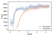
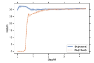
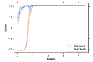
Figure 13: Natural and robustness performance exhibited by SA-DQN agents during the training process on 4 Atari games.

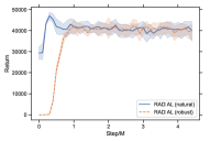
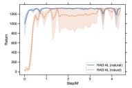
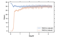
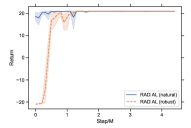
Figure 14: Natural and robustness performance exhibited by RADIAL-DQN agents during the training process on 4 Atari games.

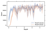
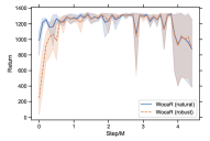
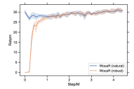
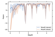
Figure 15: Natural and robustness performance exhibited by WocaR-DQN agents during the training process on 4 Atari games.

Table 8: Performance of PPO with different $k$-measurement errors.

Env	$k$-measurement	Natural Reward	Attack Reward
			Random	Critic	MAD	RS	SA-RL	PA-AD	Worst
Hopper ($\epsilon$=0.075)	$k=1$	3081	2923	2035	1763	756	79	823	79
	$k=2$	3483	3461	1506	2472	573	375	402	375
	$k=\infty$	3711	3702	3692	3473	1652	2430	2640	1652
Walker2d ($\epsilon$=0.05)	$k=1$	4622	4628	4584	4507	1062	719	336	336
	$k=2$	4738	4651	4620	4121	923	1571	424	424
	$k=\infty$	4755	4848	5044	4637	4379	4307	4303	4303
Halfcheetah ($\epsilon$=0.15)	$k=1$	5048	4463	3281	918	1049	-213	-69	-213
	$k=2$	4370	3857	3295	956	441	-160	-192	-192
	$k=\infty$	5053	5058	5065	5051	5140	4860	4942	4860
Ant ($\epsilon$=0.15)	$k=1$	5381	5329	4696	1768	1097	-1398	-3107	-3107
	$k=2$	5485	5036	4705	1199	1001	-1470	-1108	-1470
	$k=\infty$	5029	5006	4786	4549	3553	3099	3911	3099

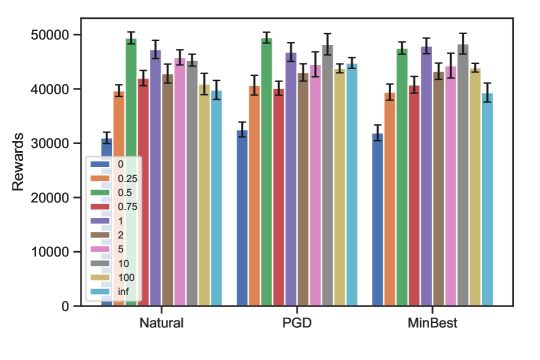
Figure 16: Natural, PGD attack and MinBest attack rewards of CAR-DQN with different soft coefficients on RoadRunner.

RoadRunner

BankHeist

Robust

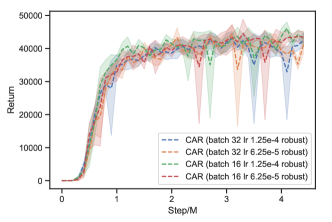
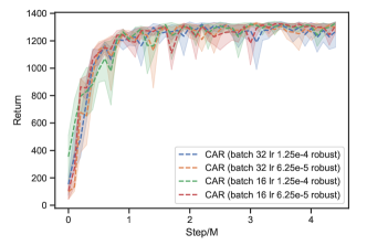
Natural

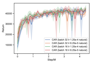
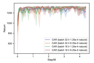
Figure 17: Episode rewards of CAR-DQN with different batch sizes and learning rates during training on RoadRunner and BankHeist with and without PGD attack.

Insensitivity of Learning Rate and Batch Size. We compare the performance of CAR-DQN with different small batch size $(16,32)$ and learning rate $(1.25\times 10^{-4},6.25\times 10^{-5})$ which are respectively used by Zhang et al. (2020b); Liang et al. (2022). As shown in Figure 17, we can see CAR-DQN is insensitive to these parameters.

H.2 Comparisons and Analysis between RADIAL-DQN and CAR-DQN with Increasing Perturbation Radius

The core at RADIAL-DQN is a heuristic robust regularization that minimizes the overlap between bounds of perturbed Q values of the current action and others:

$$\mathcal{L}_{radial}\left(\theta\right)=\mathbb{E}_{\left(s,a,s^{\prime},r\right)}\left[\sum_{y}Q_{\text{diff}}(s,y)\cdot{Ovl}(s,y,\epsilon)\right],$$

where $Q_{\text{diff}}(s,y)=\max(0,Q(s,a)-Q(s,y)),\ Ovl(s,y,\epsilon)=\max(0,\bar{Q}(s,y,\epsilon)-\underline{Q}(s,a,\epsilon)+\eta)$ and $\eta=c\cdot Q_{\text{diff}}(s,y),c=0.5$. $Q_{\text{diff}}$ is treated as a constant for the optimization. We consider RADIAL-DQN could perform better than CAR-DQN with increasing perturbation radius since $\mathcal{L}_{radial}\left(\theta\right)$ is a stronger regularization to enhance robustness while compromising natural rewards. The stronger robust constraint is mainly reflected in two aspects:

• The loose bounds. RADIAL-DQN uses the cheap but loose convex relaxation method (IBP) to estimate $\bar{Q}(s,y,\epsilon)$ and $\underline{Q}(s,a,\epsilon)$.

• The positive margin $\eta$.

They both result in ${Ovl}(s,y,\epsilon)$ a stronger constraint for representing the overlap of perturbed Q values. However, RADIAL-DQN has the following weaknesses:

• $\mathcal{L}_{radial}\left(\theta\right)$ will harm natural rewards. As shown in Figure 7, the natural rewards curve of RADIAL-DQN on RoadRunner distinctly tends to decrease, especially around 0.5 million steps. In contrast, the natural curves of our CAR-DQN showcase more stable upward trends in all environments. Besides, as shown in Table 10, RADIAL-DQN training with a larger radius attains lower natural rewards which also restricts robustness according to our theory, while CAR-DQN keeps a better and consistent natural and robust performance.

• Heuristic implementation lacks theoretical guarantees and introduces sensitive hyperparameter $c$. We conduct additional experiments on RoadRunner with different $c$ and observe the sensitivity of RADIAL-DQN to the choice of $c$, as shown in Table 9. Larger $c$ could cause poor performance because the robustness constraint is too strict and thus the policy degrades to some simple policy with lower rewards. Smaller $c$ may result in much weaker robustness. By contrast, our CAR-DQN is developed based on the theory of optimal robust policy and stability. Although we also introduce a hyperparameter $\lambda$, our ablation studies in Figure 9 show that our algorithm is insensitive to the soft coefficient $\lambda$.

  Table 9: Performance of RADIAL-DQN sensitive to different positive margins $c\cdot Q_{\text{diff}}(s,y)$.

  Model	Natural Return	PGD			MinBest
  		$\epsilon=1/255$	$\epsilon=3/255$	$\epsilon=5/255$	$\epsilon=1/255$	$\epsilon=3/255$	$\epsilon=5/255$
  RADIAL-DQN ($c=0.25$)	$14678\pm 329$	$14836\pm 314$	$13670\pm 466$	$13512\pm 617$	$14712\pm 309$	$14804\pm 457$	$13226\pm 351$
  RADIAL-DQN ($c=0.5$)	$\bf 46224\pm 1133$	$\bf 45990\pm 1112$	$\bf 42162\pm 1147$	$\bf 23248\pm 499$	$\bf 46082\pm 1128$	$\bf 42036\pm 1048$	$\bf 25434\pm 756$
  RADIAL-DQN ($c=0.75$)	$3992\pm 482$	$3992\pm 482$	$3992\pm 482$	$3992\pm 482$	$3992\pm 482$	$3992\pm 482$	$3992\pm 482$

• Depending on the currently learned optimal action. $\mathcal{L}_{radial}\left(\theta\right)$ essentially takes the currently learned action as a robust label which may produce a wrong direction for robustness training if the learned action is not optimal. In contrast, our CAR-DQN seeks optimal robust policies with theoretical guarantees and does not utilize the learned action for robustness training, simultaneously improving natural and robust performance.

The main motivation of CAR-DQN based on our theory is to improve natural and robust performance concurrently which makes sense in real-world scenarios where strong adversarial attacks are relatively rare. Our training loss can guarantee robustness under the attack with the same perturbation radius as the training. We also think it is a very significant problem whether and how we can design an algorithm training with little epsilon and theoretically guarantee robustness for larger epsilon. However, this is beyond the scope of our paper and we will consider this problem in subsequent work.

Moreover, as shown in Table 7, CAR-DQN also achieves the top performance in larger perturbation radiuses on Pong and BankHeist and matches the RADIAL-DQN on Freeway. To show the superiority of CAR-DQN further, we also train CAR-DQN with a perturbation radius of 3/255 and 5/255 on RoadRunner for 4.5 million steps (see Table 10).

Table 10: Performance of CAR-DQN and RADIAL-DQN trained with different perturbation radiuses on the RoadRunner environment. The best results of the algorithm with the same training radius are highlighted in bold.

Model	Natural Return	PGD			MinBest
		$\epsilon=1/255$	$\epsilon=3/255$	$\epsilon=5/255$	$\epsilon=1/255$	$\epsilon=3/255$	$\epsilon=5/255$
RADIAL-DQN ($\epsilon=1/255$)	$46224\pm 1133$	$45990\pm 1112$	$\bf 42162\pm 1147$	$\bf 23248\pm 499$	$46082\pm 1128$	$\bf 42036\pm 1048$	$\bf 25434\pm 756$
CAR-DQN ($\epsilon=1/255$)	$\bf 49398\pm 1106$	$\bf 49456\pm 992$	$28588\pm 1575$	$15592\pm 885$	$\bf 47526\pm 1132$	$32878\pm 1898$	$21102\pm 1427$
RADIAL-DQN ($\epsilon=3/255$)	$34656\pm 1104$	$35094\pm 1277$	$35082\pm 948$	$\bf 32770\pm 1062$	$35096\pm 1277$	$34374\pm 996$	$\bf 27926\pm 881$
CAR-DQN ($\epsilon=3/255$)	$\bf 47348\pm 1305$	$\bf 46284\pm 1114$	$\bf 43578\pm 1315$	$27060\pm 1117$	$\bf 46286\pm 1122$	$\bf 42602\pm 1336$	$24862\pm 1195$
RADIAL-DQN ($\epsilon=5/255$)	$35160\pm 1157$	$36158\pm 1104$	$36732\pm 1076$	$34826\pm 913$	$36158\pm 1104$	$36732\pm 1076$	$34592\pm 913$
CAR-DQN ($\epsilon=5/255$)	$\bf 42545\pm 2028$	$\bf 43230\pm 1468$	$\bf 37845\pm 2344$	$\bf 39235\pm 1519$	$\bf 43645\pm 1531$	$\bf 37535\pm 2112$	$\bf 38150\pm 1316$

We can see that CAR-DQN still attains superior natural and robust performance training with larger attack radiuses while RADIAL-DQN markedly degrades its natural performance due to the too-strong robustness constraint. CAR-DQN always has a higher robust return on the training radius than RADIAL-DQN.

References

- Behzadan and Munir (2017a) Vahid Behzadan and Arslan Munir. Vulnerability of deep reinforcement learning to policy induction attacks. In Machine Learning and Data Mining in Pattern Recognition: 13th International Conference, MLDM 2017, New York, NY, USA, July 15-20, 2017, Proceedings 13, pages 262–275. Springer, 2017a.
- Behzadan and Munir (2017b) Vahid Behzadan and Arslan Munir. Whatever does not kill deep reinforcement learning, makes it stronger. arXiv preprint arXiv:1712.09344, 2017b.
- Bharti et al. (2022) Shubham Bharti, Xuezhou Zhang, Adish Singla, and Jerry Zhu. Provable defense against backdoor policies in reinforcement learning. Advances in Neural Information Processing Systems, 35:14704–14714, 2022.
- Brockman et al. (2016) Greg Brockman, Vicki Cheung, Ludwig Pettersson, Jonas Schneider, John Schulman, Jie Tang, and Wojciech Zaremba. Openai gym. arXiv preprint arXiv:1606.01540, 2016.
- Bukharin et al. (2024) Alexander Bukharin, Yan Li, Yue Yu, Qingru Zhang, Zhehui Chen, Simiao Zuo, Chao Zhang, Songan Zhang, and Tuo Zhao. Robust multi-agent reinforcement learning via adversarial regularization: Theoretical foundation and stable algorithms. Advances in Neural Information Processing Systems, 36, 2024.
- Fischer et al. (2019) Marc Fischer, Matthew Mirman, Steven Stalder, and Martin Vechev. Online robustness training for deep reinforcement learning. arXiv preprint arXiv:1911.00887, 2019.
- Franzmeyer et al. (2024) Tim Franzmeyer, Stephen Marcus McAleer, Joao F Henriques, Jakob Nicolaus Foerster, Philip Torr, Adel Bibi, and Christian Schroeder de Witt. Illusory attacks: Information-theoretic detectability matters in adversarial attacks. In The Twelfth International Conference on Learning Representations, 2024.
- Gelfand and Mitter (1991) Saul B Gelfand and Sanjoy K Mitter. Recursive stochastic algorithms for global optimization in rˆd. SIAM Journal on Control and Optimization, 29(5):999–1018, 1991.
- Ghosh et al. (2020) Dibya Ghosh, Marlos C Machado, and Nicolas Le Roux. An operator view of policy gradient methods. Advances in Neural Information Processing Systems, 33:3397–3406, 2020.
- Gleave et al. (2020) Adam Gleave, Michael Dennis, Cody Wild, Neel Kant, Sergey Levine, and Stuart Russell. Adversarial policies: Attacking deep reinforcement learning. In International Conference on Learning Representations, 2020. URL https://openreview.net/forum?id=HJgEMpVFwB.
- Goodfellow et al. (2015) Ian J Goodfellow, Jonathon Shlens, and Christian Szegedy. Explaining and harnessing adversarial examples. In International Conference on Learning Representations, 2015.
- Gowal et al. (2019) Sven Gowal, Krishnamurthy Dj Dvijotham, Robert Stanforth, Rudy Bunel, Chongli Qin, Jonathan Uesato, Relja Arandjelovic, Timothy Mann, and Pushmeet Kohli. Scalable verified training for provably robust image classification. In Proceedings of the IEEE/CVF International Conference on Computer Vision, pages 4842–4851, 2019.
- Guo et al. (2023) Junfeng Guo, Ang Li, Lixu Wang, and Cong Liu. Policycleanse: Backdoor detection and mitigation for competitive reinforcement learning. In Proceedings of the IEEE/CVF International Conference on Computer Vision, pages 4699–4708, 2023.
- He et al. (2023) Sihong He, Songyang Han, Sanbao Su, Shuo Han, Shaofeng Zou, and Fei Miao. Robust multi-agent reinforcement learning with state uncertainty. Transactions on Machine Learning Research, 2023. ISSN 2835-8856. URL https://openreview.net/forum?id=CqTkapZ6H9.
- Huang et al. (2017) Sandy Huang, Nicolas Papernot, Ian Goodfellow, Yan Duan, and Pieter Abbeel. Adversarial attacks on neural network policies. arXiv preprint arXiv:1702.02284, 2017.
- Ibarz et al. (2021) Julian Ibarz, Jie Tan, Chelsea Finn, Mrinal Kalakrishnan, Peter Pastor, and Sergey Levine. How to train your robot with deep reinforcement learning: lessons we have learned. The International Journal of Robotics Research, 40(4-5):698–721, 2021.
- Ilahi et al. (2021) Inaam Ilahi, Muhammad Usama, Junaid Qadir, Muhammad Umar Janjua, Ala Al-Fuqaha, Dinh Thai Hoang, and Dusit Niyato. Challenges and countermeasures for adversarial attacks on deep reinforcement learning. IEEE Transactions on Artificial Intelligence, 3(2):90–109, 2021.
- Inkawhich et al. (2020) Matthew Inkawhich, Yiran Chen, and Hai Li. Snooping attacks on deep reinforcement learning. In Proceedings of the 19th International Conference on Autonomous Agents and MultiAgent Systems, AAMAS ’20, page 557–565, Richland, SC, 2020. International Foundation for Autonomous Agents and Multiagent Systems. ISBN 9781450375184.
- Kingma and Ba (2015) Diederik P. Kingma and Jimmy Ba. Adam: A method for stochastic optimization. In International Conference on Learning Representations, 2015. URL https://openreview.net/forum?id=8gmWwjFyLj.
- Kiourti et al. (2020) Panagiota Kiourti, Kacper Wardega, Susmit Jha, and Wenchao Li. Trojdrl: evaluation of backdoor attacks on deep reinforcement learning. In 2020 57th ACM/IEEE Design Automation Conference (DAC), pages 1–6. IEEE, 2020.
- Kiran et al. (2021) B Ravi Kiran, Ibrahim Sobh, Victor Talpaert, Patrick Mannion, Ahmad A Al Sallab, Senthil Yogamani, and Patrick Pérez. Deep reinforcement learning for autonomous driving: A survey. IEEE Transactions on Intelligent Transportation Systems, 23(6):4909–4926, 2021.
- Korkmaz (2023) Ezgi Korkmaz. Adversarial robust deep reinforcement learning requires redefining robustness. In Proceedings of the AAAI Conference on Artificial Intelligence, volume 37, pages 8369–8377, 2023.
- Kos and Song (2017) Jernej Kos and Dawn Song. Delving into adversarial attacks on deep policies. arXiv preprint arXiv:1705.06452, 2017.
- Kumar et al. (2022) Aounon Kumar, Alexander Levine, and Soheil Feizi. Policy smoothing for provably robust reinforcement learning. In International Conference on Learning Representations, 2022. URL https://openreview.net/forum?id=mwdfai8NBrJ.
- Li et al. (2024) Haoran Li, Zicheng Zhang, Wang Luo, Congying Han, Yudong Hu, Tiande Guo, and Shichen Liao. Towards optimal adversarial robust q-learning with Bellman infinity-error. In Ruslan Salakhutdinov, Zico Kolter, Katherine Heller, Adrian Weller, Nuria Oliver, Jonathan Scarlett, and Felix Berkenkamp, editors, Proceedings of the 41st International Conference on Machine Learning, volume 235 of Proceedings of Machine Learning Research, pages 29324–29372. PMLR, 21–27 Jul 2024. URL https://proceedings.mlr.press/v235/li24cl.html.
- Liang et al. (2022) Yongyuan Liang, Yanchao Sun, Ruijie Zheng, and Furong Huang. Efficient adversarial training without attacking: Worst-case-aware robust reinforcement learning. Advances in Neural Information Processing Systems, 35:22547–22561, 2022.
- Liang et al. (2024) Yongyuan Liang, Yanchao Sun, Ruijie Zheng, Xiangyu Liu, Benjamin Eysenbach, Tuomas Sandholm, Furong Huang, and Stephen Marcus McAleer. Game-theoretic robust reinforcement learning handles temporally-coupled perturbations. In The Twelfth International Conference on Learning Representations, 2024. URL https://openreview.net/forum?id=wZWTHU7AsQ.
- Lillicrap et al. (2016) Timothy P. Lillicrap, Jonathan J. Hunt, Alexander Pritzel, Nicolas Heess, Tom Erez, Yuval Tassa, David Silver, and Daan Wierstra. Continuous control with deep reinforcement learning. In International Conference on Learning Representations, 2016. URL https://openreview.net/forum?id=kJP8gA8BxRY.
- Lin et al. (2017) Yen-Chen Lin, Zhang-Wei Hong, Yuan-Hong Liao, Meng-Li Shih, Ming-Yu Liu, and Min Sun. Tactics of adversarial attack on deep reinforcement learning agents. In International Joint Conference on Artificial Intelligence, pages 3756–3762, 2017. URL https://doi.org/10.24963/ijcai.2017/525.
- Liu et al. (2024a) Xiangyu Liu, Souradip Chakraborty, Yanchao Sun, and Furong Huang. Rethinking adversarial policies: A generalized attack formulation and provable defense in RL. In The Twelfth International Conference on Learning Representations, 2024a. URL https://openreview.net/forum?id=pDCublKPmG.
- Liu et al. (2024b) Xiangyu Liu, Chenghao Deng, Yanchao Sun, Yongyuan Liang, and Furong Huang. Beyond worst-case attacks: Robust RL with adaptive defense via non-dominated policies. In The Twelfth International Conference on Learning Representations, 2024b. URL https://openreview.net/forum?id=DFTHW0MyiW.
- Lu et al. (2023) Chris Lu, Timon Willi, Alistair Letcher, and Jakob Nicolaus Foerster. Adversarial cheap talk. In International Conference on Machine Learning, pages 22917–22941. PMLR, 2023.
- Madry et al. (2018) Aleksander Madry, Aleksandar Makelov, Ludwig Schmidt, Dimitris Tsipras, and Adrian Vladu. Towards deep learning models resistant to adversarial attacks. In International Conference on Learning Representations, 2018. URL https://openreview.net/forum?id=rJzIBfZAb.
- Mnih et al. (2015) Volodymyr Mnih, Koray Kavukcuoglu, David Silver, Andrei A Rusu, Joel Veness, Marc G Bellemare, Alex Graves, Martin Riedmiller, Andreas K Fidjeland, Georg Ostrovski, et al. Human-level control through deep reinforcement learning. Nature, 518(7540):529–533, 2015.
- Mnih et al. (2016) Volodymyr Mnih, Adria Puigdomenech Badia, Mehdi Mirza, Alex Graves, Timothy Lillicrap, Tim Harley, David Silver, and Koray Kavukcuoglu. Asynchronous methods for deep reinforcement learning. In International Conference on Machine Learning, pages 1928–1937. PMLR, 2016.
- Nie et al. (2024) Buqing Nie, Jingtian Ji, Yangqing Fu, and Yue Gao. Improve robustness of reinforcement learning against observation perturbations via lipschitz policy networks. In Proceedings of the AAAI Conference on Artificial Intelligence, volume 38, pages 14457–14465, 2024.
- Oikarinen et al. (2021) Tuomas Oikarinen, Wang Zhang, Alexandre Megretski, Luca Daniel, and Tsui-Wei Weng. Robust deep reinforcement learning through adversarial loss. Advances in Neural Information Processing Systems, 34:26156–26167, 2021.
- Pattanaik et al. (2018) Anay Pattanaik, Zhenyi Tang, Shuijing Liu, Gautham Bommannan, and Girish Chowdhary. Robust deep reinforcement learning with adversarial attacks. In International Conference on Autonomous Agents and Multiagent Systems, pages 2040–2042, 2018. URL http://dl.acm.org/citation.cfm?id=3238064.
- Schulman et al. (2015) John Schulman, Sergey Levine, Pieter Abbeel, Michael Jordan, and Philipp Moritz. Trust region policy optimization. In International Conference on Machine Learning, pages 1889–1897. PMLR, 2015.
- Schulman et al. (2016) John Schulman, Philipp Moritz, Sergey Levine, Michael Jordan, and Pieter Abbeel. High-dimensional continuous control using generalized advantage estimation. In International Conference on Learning Representations, 2016.
- Schulman et al. (2017) John Schulman, Filip Wolski, Prafulla Dhariwal, Alec Radford, and Oleg Klimov. Proximal policy optimization algorithms. arXiv preprint arXiv:1707.06347, 2017.
- Shen et al. (2020) Qianli Shen, Yan Li, Haoming Jiang, Zhaoran Wang, and Tuo Zhao. Deep reinforcement learning with robust and smooth policy. In International Conference on Machine Learning, pages 8707–8718. PMLR, 2020.
- Silver et al. (2014) David Silver, Guy Lever, Nicolas Heess, Thomas Degris, Daan Wierstra, and Martin Riedmiller. Deterministic policy gradient algorithms. In International Conference on Machine Learning, pages 387–395. PMLR, 2014.
- Silver et al. (2016) David Silver, Aja Huang, Chris J Maddison, Arthur Guez, Laurent Sifre, George Van Den Driessche, Julian Schrittwieser, Ioannis Antonoglou, Veda Panneershelvam, Marc Lanctot, et al. Mastering the game of go with deep neural networks and tree search. Nature, 529(7587):484–489, 2016.
- Sun et al. (2024) Chung-En Sun, Sicun Gao, and Tsui-Wei Weng. Breaking the barrier: Enhanced utility and robustness in smoothed DRL agents. In Ruslan Salakhutdinov, Zico Kolter, Katherine Heller, Adrian Weller, Nuria Oliver, Jonathan Scarlett, and Felix Berkenkamp, editors, Proceedings of the 41st International Conference on Machine Learning, volume 235 of Proceedings of Machine Learning Research, pages 46957–46987. PMLR, 21–27 Jul 2024. URL https://proceedings.mlr.press/v235/sun24b.html.
- Sun and Zheng (2024) Xiaolin Sun and Zizhan Zheng. Belief-enriched pessimistic q-learning against adversarial state perturbations. In The Twelfth International Conference on Learning Representations, 2024. URL https://openreview.net/forum?id=7gDENzTzw1.
- Sun et al. (2022) Yanchao Sun, Ruijie Zheng, Yongyuan Liang, and Furong Huang. Who is the strongest enemy? towards optimal and efficient evasion attacks in deep RL. In International Conference on Learning Representations, 2022. URL https://openreview.net/forum?id=JM2kFbJvvI.
- Sutton (1988) Richard S Sutton. Learning to predict by the methods of temporal differences. Machine Learning, 3:9–44, 1988.
- Sutton and Barto (2018) Richard S Sutton and Andrew G Barto. Reinforcement learning: An introduction. MIT press, 2018.
- Todorov et al. (2012) Emanuel Todorov, Tom Erez, and Yuval Tassa. Mujoco: A physics engine for model-based control. In 2012 IEEE/RSJ International Conference on Intelligent Robots and Systems, pages 5026–5033. IEEE, 2012.
- Van Hasselt et al. (2016) Hado Van Hasselt, Arthur Guez, and David Silver. Deep reinforcement learning with double q-learning. In Proceedings of the AAAI Conference on Artificial Intelligence, volume 30, 2016.
- Wang et al. (2022) Chuwei Wang, Shanda Li, Di He, and Liwei Wang. Is physics informed loss always suitable for training physics informed neural network? Advances in Neural Information Processing Systems, 35:8278–8290, 2022.
- Wang et al. (2021) Lun Wang, Zaynah Javed, Xian Wu, Wenbo Guo, Xinyu Xing, and Dawn Song. Backdoorl: Backdoor attack against competitive reinforcement learning. In International Joint Conference on Artificial Intelligence, pages 3699–3705, 2021. URL https://doi.org/10.24963/ijcai.2021/509.
- Wang et al. (2016) Ziyu Wang, Tom Schaul, Matteo Hessel, Hado Hasselt, Marc Lanctot, and Nando Freitas. Dueling network architectures for deep reinforcement learning. In International Conference on Machine Learning, pages 1995–2003. PMLR, 2016.
- Weng et al. (2019) Tsui-Wei Weng, Krishnamurthy Dj Dvijotham, Jonathan Uesato, Kai Xiao, Sven Gowal, Robert Stanforth, and Pushmeet Kohli. Toward evaluating robustness of deep reinforcement learning with continuous control. In International Conference on Learning Representations, 2019.
- Williams (1992) Ronald J Williams. Simple statistical gradient-following algorithms for connectionist reinforcement learning. Machine Learning, 8:229–256, 1992.
- Wu et al. (2022) Fan Wu, Linyi Li, Zijian Huang, Yevgeniy Vorobeychik, Ding Zhao, and Bo Li. CROP: Certifying robust policies for reinforcement learning through functional smoothing. In International Conference on Learning Representations, 2022. URL https://openreview.net/forum?id=HOjLHrlZhmx.
- Yu et al. (2021) Chao Yu, Jiming Liu, Shamim Nemati, and Guosheng Yin. Reinforcement learning in healthcare: A survey. ACM Computing Surveys (CSUR), 55(1):1–36, 2021.
- Zhang et al. (2022) Bohang Zhang, Du Jiang, Di He, and Liwei Wang. Rethinking lipschitz neural networks and certified robustness: A boolean function perspective. Advances in Neural Information Processing Systems, 35:19398–19413, 2022.
- Zhang et al. (2020a) Huan Zhang, Hongge Chen, Chaowei Xiao, Sven Gowal, Robert Stanforth, Bo Li, Duane Boning, and Cho-Jui Hsieh. Towards stable and efficient training of verifiably robust neural networks. In International Conference on Learning Representations, 2020a. URL https://openreview.net/forum?id=Skxuk1rFwB.
- Zhang et al. (2020b) Huan Zhang, Hongge Chen, Chaowei Xiao, Bo Li, Mingyan Liu, Duane Boning, and Cho-Jui Hsieh. Robust deep reinforcement learning against adversarial perturbations on state observations. Advances in Neural Information Processing Systems, 33:21024–21037, 2020b.
- Zhang et al. (2021) Huan Zhang, Hongge Chen, Duane S Boning, and Cho-Jui Hsieh. Robust reinforcement learning on state observations with learned optimal adversary. In International Conference on Learning Representations, 2021. URL https://openreview.net/forum?id=sCZbhBvqQaU.
- Zhang (2023) Tong Zhang. Mathematical Analysis of Machine Learning Algorithms. Cambridge University press, 2023.
- Zheng et al. (2018) Guanjie Zheng, Fuzheng Zhang, Zihan Zheng, Yang Xiang, Nicholas Jing Yuan, Xing Xie, and Zhenhui Li. Drn: A deep reinforcement learning framework for news recommendation. In Proceedings of the 2018 World Wide Web Conference, WWW ’18, page 167–176, Republic and Canton of Geneva, CHE, 2018. International World Wide Web Conferences Steering Committee. ISBN 9781450356398. doi: 10.1145/3178876.3185994. URL https://doi.org/10.1145/3178876.3185994.