Tarski Lower Bounds from Multi-Dimensional Herringbones

Abstract

Tarski’s theorem states that every monotone function from a complete lattice to itself has a fixed point. We analyze the query complexity of finding such a fixed point on the $k$-dimensional grid of side length $n$ under the $\leq$ relation. In this setting, there is an unknown monotone function $f:\{0,1,\ldots,n-1\}^{k}\to\{0,1,\ldots,n-1\}^{k}$ and an algorithm must query a vertex $v$ to learn $f(v)$. The goal is to find a fixed point of $f$ using as few oracle queries as possible.

We show that the randomized query complexity of this problem is $\Omega\left(\frac{k\cdot\log^{2}{n}}{\log{k}}\right)$ for all $n,k\geq 2$. This unifies and improves upon two prior results: a lower bound of $\Omega(\log^{2}{n})$ from [EPRY19] and a lower bound of $\Omega\left(\frac{k\cdot\log{n}}{\log{k}}\right)$ from [BPR24], respectively.

1 Introduction

Let $\mathcal{L}$ be a complete lattice under the $\leq$ relation. A function $f:\mathcal{L}\to\mathcal{L}$ is monotone if $x\leq y$ implies $f(x)\leq f(y)$ for all $x,y\in\mathcal{L}$. Tarski’s theorem [Tar55] states that every such function has a fixed point. Tarski’s theorem has applications in many areas. In game theory, pure Nash equilibria in supermodular games can be viewed as fixed points of monotone functions, and hence by Tarski’s theorem such equilibria exist [EPRY19]. In denotational semantics, the semantics of recursively defined programs can be characterized as the least fixed points of monotone functions, ensuring a well-defined interpretation of recursion [For05].

Recently, the computational complexity of finding Tarski fixed points has been investigated for grids. Specifically, for $k,n\in\mathbb{N}$, consider the $k$-dimensional grid $\{0,\ldots,n-1\}^{k}$ of side length $n$. Let $\leq$ be the binary relation where for each pair of vertices ${a}=(a_{1},\ldots,a_{k})\in\{0,\ldots,n-1\}^{k}$ and ${b}=(b_{1},\ldots,b_{k})\in\{0,\ldots,n-1\}^{k}$, we have ${a}\leq{b}$ if and only if $a_{i}\leq b_{i}$ for each $i\in[k]$.

In the query model, there is an unknown monotone function $f:\{0,\ldots,n-1\}^{k}\to\{0,\ldots,n-1\}^{k}$. The problem $TARSKI(n,k)$ is to find a fixed point of $f$ given query access to the function, where the answer to each query $v\in\{0,\ldots,n-1\}^{k}$ is $f(v)$. The randomized query complexity is the minimum expected number of queries required to find a solution with a probability at least $9/10$, where the expectation is taken over the coin tosses of the algorithm.

There are two main algorithmic approaches for finding a Tarski fixed point on grids. One approach is a path-following method that uses $O(nk)$ queries, which is best for small $n$ and large $k$. For large $n$ and small $k$, a divide-and-conquer approach works much better. Originally proposed by [DQY11] and subsequently improved by [FPS22] and [CL22], it achieves an upper bound of $O\left((\log{n})^{\lceil\frac{k+1}{2}\rceil}\right)$ queries for any constant $k$.

There are a few known lower bounds which are optimized for different parameter regimes. [EPRY19] proved a randomized query complexity lower bound of $\Omega\left(\log^{2}(n)\right)$ for $TARSKI(n,2)$. The same lower bound applies to $TARSKI(n,k)$ for $k\geq 2$. This lower bound matches the known upper bound for $k=2$ and $k=3$, though it does not scale with $k$. [BPR24] proved two dimension-dependent randomized lower bounds, of $\Omega(k)$ and $\Omega\left(\frac{k\log n}{\log k}\right)$, respectively, for $TARSKI(n,k)$. These bounds scale with $k$, so they are stronger than [EPRY19] when $k$ grows at about $\text{polylog}(n)$. In particular, they characterize the randomized query complexity of finding a Tarski fixed point on the Boolean hypercube $\{0,1\}^{k}$ (i.e. the power set lattice) as $\Theta(k)$. However, they are weaker than [EPRY19] for very small $k$.

In this paper, we show that the randomized query complexity of $TARSKI(n,k)$ is $\Omega\left(\frac{k\log^{2}(n)}{\log k}\right)$ for all $n,k\geq 2$. This is a dimension-dependent lower bound that unifies and improves upon the lower bounds of $\Omega\left(\log^{2}(n)\right)$ from [EPRY19] and of $\Omega\left(\frac{k\log n}{\log k}\right)$ from [BPR24].

1.1 Our Contribution

Our main result is the following theorem.

Theorem 1.

There exists $c>0$ such that for all $k,n\in\mathbb{N}$ with $k,n\geq 2$, the randomized query complexity of $TARSKI(n,k)$ is at least $c\cdot\frac{k\log^{2}{n}}{\log{k}}$.

Proof Overview. Our first contribution is to design a multi-dimensional family $\mathcal{F}$ of herringbone functions, which generalizes the 2D construction from [EPRY19].

At a high level, there is a path (“spine”) that runs from vertex $(0,\ldots,0)$ to $(n-1,\ldots,n-1)$ that contains the unique fixed point. Along the spine, function values flow directly towards the fixed point. Outside the spine, the function is designed to be consistent with any position of the fixed point along the spine, which forces the algorithm to find “many” spine vertices to succeed. The challenge we overcome is defining such a function in a way that explicitly uses all the dimensions without violating monotonicity.

To obtain a lower bound, we invoke Yao’s lemma, which allows focusing on a deterministic algorithm $\mathcal{A}$ that receives inputs drawn from the uniform distribution $\mathcal{U}$ over functions from $\mathcal{F}$. The high level idea is that distribution $\mathcal{U}$ has the property that the location of each spine vertex is independent of spine vertices more than a short distance away. Consequently, a successful algorithm must repeatedly find spine vertices without relying on previously discovered ones, and finding each new spine vertex requires “many” queries.

Formalizing this intuition requires careful handling. We design a monotonic measure of progress that starts with a low value, increases by a small amount in expectation with each query, and must arrive at a high value for $\mathcal{A}$ to succeed. To do so, we first divide the space around the spine into regions. For each region $R$, we define random variables:

• $P_{t}(R)=\max_{v\in R}\log_{2}\Pr\left[\text{$v$ is a spine vertex after $t$ queries from $\mathcal{A}$}\right]$ for all $t\in\mathbb{N}$.

• $P^{*}_{t}(R)=\max_{0\leq t^{*}\leq t}P_{t^{*}}(R)$ for all $t\in\mathbb{N}$.

For $m\in\Theta(\log n)$, let $G_{m}$ be the set of $m$-tuples of regions that are sufficiently far apart from each other that the location of the spine in each region is independent of the others in the tuple. Define

• $\overline{P}_{t}=\max_{(R^{1},\ldots,R^{m})\in G_{m}}\sum_{i=1}^{m}P^{*}_{t}(R^{i})$ for all $t\in\mathbb{N}$.

The proof shows that $\overline{P}$ is a monotonic measure of progress with the required properties, which implies a lower bound on the number of queries needed for the algorithm to succeed.

Roadmap to the paper.

The remainder of the paper is organized as follows. Related work is in Section 1.2. The model and preliminaries are in Section 2.

Our family $\mathcal{F}$ of multi-dimensional herringbone functions can be found in Section 3, with proofs of its properties in Appendix A. In Section 4 we define a distribution $\mathcal{U}$ on the family of functions $\mathcal{F}$, with proofs of its properties in Appendix B. The proof of Theorem 1 can be found in Section 5, with proofs of supporting lemmas in Appendix C.

In Section 6 we also give upper bounds on the query complexity of finding a fixed point of any multi-dimensional herringbone function.

1.2 Related Work

Algorithms for the problem of finding Tarski fixed points on the $k$-dimensional grid of side length $n$ have only recently been considered. [DQY20] gave an $O(\log^{k}(n))$ divide-and-conquer algorithm. [FPS22] gave an $O(\log^{2}(n))$ algorithm for the 3D grid and used it to construct an $O(\log^{2\lceil k/3\rceil}(n))$ algorithm for the $k$-dimensional grid of side length $n$. [CL22] extended their ideas to get an $O(\log^{\lceil(k+1)/2\rceil}(n))$ algorithm.

[EPRY19] showed a lower bound of $\Omega(\log^{2}(n))$ for the 2D grid, implying the same lower bound for the $k$-dimensional grid of side length $n$. This bound is tight for $k=2$ and $k=3$, but there is an exponential gap for larger $k$. They also showed that the problem is in both PLS and PPAD, which by the results of [FGHS22] implies it is in CLS.

[CLY23] give a black-box reduction from the Tarski problem to the same problem with an additional promise that the input function has a unique fixed point. This result implies that the Tarski problem and the unique Tarski problem have the same query complexity.

Two problems related conceptually to that of finding a Tarski fixed point are finding a Brouwer fixed point [HPV89, CD05, CT07] and finding a local minimum (i.e. local search) [Ald83, Aar06, Zha09, LTT89, SY09, SS04, DR10]. The query complexity lower bounds for Brouwer and local search also rely on hidden path (“spine”) constructions. However, the monotonicity condition of the function in the Tarski setting poses an extra challenge.

2 Model

Let $\{0,1,\ldots,n-1\}^{k}$ be the $k$-dimensional grid of side length $n$ under the $\leq$ relation. Given oracle access to an (unknown) monotone function $f:\{0,1,\ldots,n-1\}^{k}\to\{0,1,\ldots,n-1\}^{k}$, the Tarski search problem, ${TARSKI}(n,k)$, is to find a fixed point of $f$ using as few oracle queries as possible.

Definition 1 (${TARSKI}(n,k)$).

Let $k,n\in\mathbb{N}$. Given oracle access to an unknown monotone function $f:\{0,1,\ldots,n-1\}^{k}\to\{0,1,\ldots,n-1\}^{k}$, find a vertex $x\in\{0,1,\ldots,n-1\}^{k}$ with $f(x)=x$ using as few queries as possible.

Query complexity.

The deterministic query complexity of a task is the total number of queries necessary and sufficient for a correct deterministic algorithm to find a solution. The randomized query complexity is the expected number of queries required to find a solution with probability at least 9/10 for each input , where the expectation is taken over the coin tosses of the algorithm.

Given an algorithm $\mathcal{A}$ for $TARSKI(n,k)$ that receives an input drawn from some input distribution $\mathcal{D}$, we say that an execution of $\mathcal{A}$ succeeds if it outputs a fixed point of the function given as input and fails otherwise.

Notation. The following notation is used throughout the paper.

• For a vector $\mathbf{x}$ in $\mathbb{R}^{k}$ and $i\in[k]$, we write the $i$-th coordinate of $\mathbf{x}$ as $x_{i}$.

• For a vector $\mathbf{x}\in\mathbb{R}^{k}$, we use $wt(\mathbf{x})$ to denote its Hamming weight $\sum_{i=1}^{k}x_{i}$.

• For each $j\in[k]$, let $\mathbf{e}_{j}=(0,\ldots,0,1,0,\ldots,0)$, where the vector $\mathbf{e}_{j}$ is all zeroes except the $j$-th coordinate in which it takes value $1$.

• For all $u,v\in\mathbb{R}^{k}$, the line segment between them is $\ell(u,v)=\bigl{\{}\lambda u+(1-\lambda)v\mid\lambda\in[0,1]\bigr{\}}\,.$

3 Multi-dimensional Herringbone Functions

Our first contribution is to generalize the lower bound construction from [EPRY19] to any number of dimensions. Towards this end, we need to state the definition of a spine, which is a monotone sequence of vertices that each have Hamming distance $1$ from their neighbors.

Definition 2 (Spine).

A spine $\mathbf{s}=\{s^{0},\ldots,s^{(n-1)k}\}$ is a sequence of vertices with the property that $s^{0}=(0,\ldots,0)$, $s^{(n-1)k}=(n-1,\ldots,n-1)$, and $s^{i+1}>s^{i}$ for all $i\in\{0,\ldots,(n-1)k-1\}$.

Lemma 1.

Let $\mathbf{s}=(s^{0},\ldots,s^{(n-1)k})$ be a spine. Then $wt(s^{i})=i$ for each $i\in\{0,\ldots,(n-1)k\}$.

Proof.

By the definition of a spine, we have $s^{i+1}>s^{i}$ for all $i\in\{0,\ldots,(n-1)k-1\}$. Thus $wt(s^{i+1})>wt(s^{i})$. The available Hamming weights are $\{0,\ldots,k(n-1)\}$, thus $wt(s^{i})=i$ for all $i\in\{0,\ldots,(n-1)k\}$. ∎

Definition 3 (Multi-dimensional Herringbone Function).

Consider a spine $\mathbf{s}=\{s^{0},\ldots,s^{(n-1)k}\}$ and an index $j\in\{0,\ldots,(n-1)k\}$. Define functions $M,\mu:\{0,\ldots,n-1\}^{k}\to\{0,\ldots,(n-1)k\}$ as:

$$M(v)=\min\left\{i\in\{0,\ldots,(n-1)k\}\mid s^{i}\geq v\right\}\;\;\;\mbox{and}\;\;\;\mu(v)=\max\left\{i\in\{0,\ldots,(n-1)k\}\mid s^{i}\leq v\right\}\,.$$

Let $h^{\mathbf{s},j}:\{0,\ldots,n-1\}^{k}\to\{0,\ldots,n-1\}^{k}$ be the function:

$$h^{\mathbf{s},j}(v)=\begin{cases}v&\text{if }v=s^{j}\\ s^{i+1}&\text{if }v=s^{i}\text{ for some }i<j\\ s^{i-1}&\text{if }v=s^{i}\text{ for some }i>j\\ v+(s^{\mu(v)+1}-s^{\mu(v)})-(s^{M(v)}-s^{M(v)-1})&\text{otherwise}\,.\end{cases}$$ (1)

The first three cases of Definition 3 are the same as in the two-dimensional construction of [EPRY19], as they naturally extend to the higher-dimensional setting without modification.

Our key innovation lies in the fourth case, which applies to vertices not on the spine. It is designed to hide the location of $s^{j}$ by being consistent with any value of $j$.

We show that each function $h^{\mathbf{s},j}$ from Definition 3 has a unique fixed point at $s^{j}$ and is monotone. The proofs are included in Appendix A.

Lemma 2.

The function $h^{\mathbf{s},j}$ in Definition 3 has a unique fixed point at $s^{j}$.

Lemma 3.

The function $h^{\mathbf{s},j}$ in Definition 3 is monotone.

On the spine, $h^{\mathbf{s},j}$ follows the spine to $s^{j}$. Off the spine, $h^{\mathbf{s},j}(v)$ increases in the dimension that the spine moves after $s^{\mu(v)}$ and decreases in the dimension that the spine moves before $s^{M(v)}$.

In two dimensions, this coincides with the herringbone function of [EPRY19]: vertices above the spine go down-right, and vertices below the spine go up-left. In higher dimensions, however, the off-spine vertices do not in general point directly at the spine.

4 Hard Distribution

In this section we define a hard distribution of inputs that is used to prove Theorem 1. We will use multi-dimensional herringbone functions with spines of a particular form. The proofs of statements in this section can be found in Appendix B.

The idea is to restrict the spine to a “tube” running from the minimum to the maximum vertex in the lattice with width $\text{poly}(n)$. We select connecting points on several slices throughout the tube and make the spine interpolate between these points.

We first introduce the tube and some of its useful properties.

Definition 4 (Tube).

The tube of width $L$ in $\{0,\ldots,n-1\}^{k}$ is the set of points:

$$T_{L}=\{x\in\{0,\ldots,n-1\}^{k}\mid\exists i\in\{0,\ldots,n-1\}\text{ such that $|x_{j}-i|\leq L$}\;\forall j\in[k]\}\,.$$ (2)

The main appeal of the tube is that queries inside the tube can only provide information about nearby spine vertices.

Lemma 4.

For a point $v\in T_{L}$ and a multi-dimensional herringbone function $f$ whose spine lies in $T_{L}$, the value of $f(v)$ depends only on spine vertices whose coordinates are all within $2L$ of $v$’s.

However, an algorithm is free to query any vertices, not just ones in the tube. We get around this by reducing a query to a vertex $v$ outside the tube to two queries on the boundary of the tube, which together provide the same information as querying $v$.

Lemma 5.

Let $L\in\mathbb{N}$ and $f:\{0,\ldots,n-1\}^{k}\to\{0,\ldots,n-1\}^{k}$ be a multi-dimensional herringbone function whose spine lies entirely in $T_{L}$. For each point $v\not\in T_{L}$, there exist $a,b\in T_{L}$ such that:

• $a$ and $b$ can be computed from $v$ and $L$; and

• $f(v)$ can be computed from $f(a)$ and $f(b)$.

We now divide the tube $T_{L}$ into regions, whose sizes are defined using a parameter $\rho\geq 0$ such that $\rho\mid k(n-1)$, $k\mid\rho$, and $\rho\geq 12kL$. We will eventually use $L=\frac{1}{12}\sqrt{n-1}$ and $\rho=k\sqrt{n-1}$, but these precise values are not important until the final bound is evaluated. We do require $L$ and $\rho$ to be integers, which will only occur if $n-1$ is the square of an integer that is divisible by $12$. However, such values of $n$ are sufficiently common that rounding down to the nearest one is a negligible loss.

We define a set of indices $a$ for the regions we focus on as follows:

$$\mathcal{I}=\Bigl{\{}a\mid a\in\{0,\ldots,k(n-1)\}\;\mbox{and}\;\rho\mid a\Bigr{\}}\,.$$ (3)

Definition 5 (Regions).

For each $a\in\mathcal{I}\setminus\{k(n-1)\}$, define the region

$$R_{a}=\{\mathbf{x}\in T_{L}\mid a\leq wt(\mathbf{x})\leq a+\rho\}\,.$$ (4)

For all $a\in\mathcal{I}$, let $Low_{a}=\{\mathbf{x}\in T_{L}\mid wt(\mathbf{x})=a\}\,.$ For each region $R_{a}$, $Low_{a}$ is its lower boundary.

The spines of our hard input distributions will be defined by passing through a series of connecting points, one at each region boundary.

Definition 6 (Connecting points).

Given $i\in\mathcal{I}$, the vertices $\chi_{i}$ are called connecting points if $\chi_{i}\in Low_{i}$.

Given a sequence of connecting points $\chi_{i}$, we next construct a spine that interpolates between them. Each $\chi_{i}$ represents the vertex that the spine passes through when entering region $R_{i}$ from $R_{i-\rho}$.

For each vertex $v\in\{0,\ldots,n-1\}^{k}$, let $\mathcal{C}(v)$ be the axis-aligned cube of side length $1$ centered at $v$. For each $i\in[k]$, the face of $\mathcal{C}(v)$ with minimum value in coordinate $i$ is called backward and the face with maximum value in coordinate $i$ is called forward.

Lemma 6.

Let $a,b\in\{0,\ldots,n-1\}^{k}$ with $a\leq b$. For an arbitrary vertex $v\in\{0,\ldots,n-1\}^{k}$, suppose the cube $\mathcal{C}(v)$ intersects the line segment $\ell(a,b)$. Let $z\in\mathbb{R}^{k}$ be such that $z=\max\{\mathcal{C}(v)\cap\ell(a,b)\}$. Then $z$ is well-defined, and either $v=b$ or $z$ lies on some forward face of $\mathcal{C}(v)$.

Lemma 7.

Let $u,v\in\{0,\ldots,n-1\}^{k}$ be vertices with $u\leq v$. Then there exists a sequence of vertices $s^{1},\ldots,s^{m}$ for some $m\in\mathbb{N}$ such that

1. $s^{1}=u$ and $s^{m}=v$.

2. $(s^{1},\ldots,s^{m})$ is a monotone connected path in the graph $\{0,\ldots,n-1\}^{k}$.

3. For each $i\in[m]$, the set $\mathcal{C}(s^{i})\cap\ell(u,v)$ is nonempty.

An illustration of the construction given by Lemma 7 can be found in Figure 1.

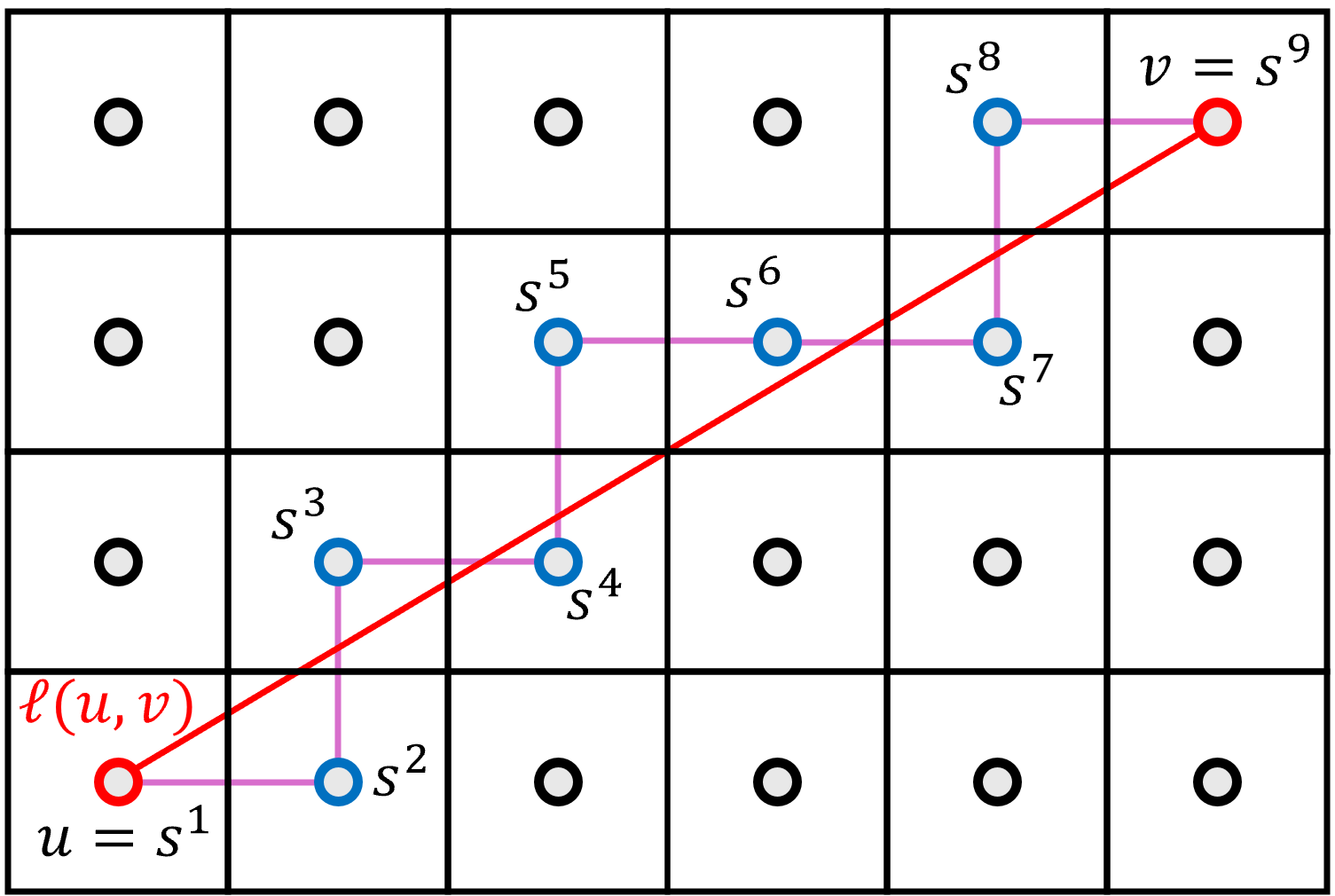
Figure 1: A 2-dimensional example of the construction of Lemma 7, with endpoints $u$ and $v$ and the associated spine vertices $s^{1}$ through $s^{9}$. Each vertex is drawn surrounded by its cube.

Definition 7 (Spine induced by connecting points).

Let $\chi_{i}$ for $i\in\mathcal{I}$ be connecting points. For each consecutive pair of connecting points $\chi_{i}$ and $\chi_{i+\rho}$, define the sequence $(s^{i},s^{i+1},\ldots,s^{i+\rho})$ as given by Lemma 7 invoked with $u=\chi_{i}$ and $v=\chi_{i+\rho}$. Let the spine be $\mathbf{s}=(s^{0},\ldots,s^{(n-1)k})$.

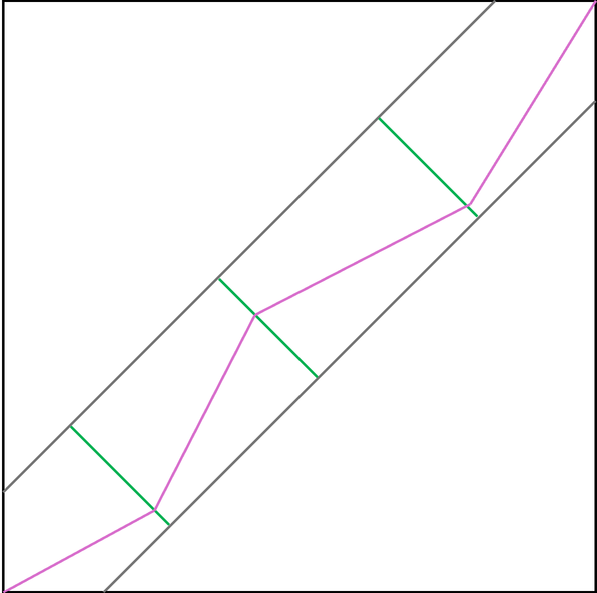
Figure 2: A sketch of the structure of the spines in Definition 7. The gray lines represent the edges of the tube $T_{L}$. The green lines represent $Low_{a}$ for various $a\in\mathcal{I}$, and divide $T_{L}$ into several regions. The pink path represents a possible spine through a choice of connecting points.

Observation 1.

Each spine $\mathbf{s}$ from Definition 7 is monotone.

Proof.

Given a set of connecting points $\chi_{i}$ for $i\in\mathcal{I}$, the spine from Definition 7 is obtained by generating a monotone path $P_{i}$ to connect each consecutive pair of connecting points $\chi_{i}$ and $\chi_{i+\rho}$. Then the spine is the union of the $P_{i}$’s and thus monotone as well. ∎

Definition 8 (Set of spines $\Psi$, family of functions $\mathcal{F}$, and distribution $\mathcal{U}$).

The set of spines we consider is

$$\Psi =\Bigl{\{}\mathbf{s}\mid\exists\mbox{ connecting points }\chi_{i}\mbox{ for }i\in\mathcal{I}\mbox{ such that }\mathbf{s}\mbox{ is the spine induced by them}\Bigr{\}}$$ (5)

The family of functions we consider is $\mathcal{F}=\bigl{\{}h^{\mathbf{s},j}\mid\mathbf{s}\in\Psi,j\in\{0,\ldots,k(n-1)\}\bigr{\}}$. Let $\mathcal{U}$ be the uniform distribution over functions in $\mathcal{F}$.

Choosing spine vertices independently in different regions allows us to show that queries within the tube truly give only local information, extending Lemma 4.

Lemma 8.

Suppose a vertex $v\in\{0,\ldots,n-1\}^{k}$ is in a region $R_{\alpha}$. On input $f\sim\mathcal{U}$, the value of $f(v)$ is independent of the location of spine vertices in all regions except possibly regions $R_{\alpha+i\rho}$ for $i\in\{-2,\ldots,2\}$.

5 Proof of the Main Theorem

We now move towards the proof of Theorem 1. At a high level, the lower bound in this theorem comes from a combination of two ideas:

• Lemma 12, which states that finding spine vertices in many different regions is difficult. Its proof is based on spine vertices being exponentially rare due to our construction.

• Lemma 13, which states that any correct algorithm for $TARSKI(n,k)$ must nevertheless find spine vertices in many different regions. Its proof is based on a reduction to ordered search.

The proofs of statements in this section can be found in Appendix C.

We begin with the ideas leading to Lemma 12. The general idea is that any given vertex is very unlikely to be a spine vertex (Lemmas 9 and 10), while each query only provides $O(\log k)$ bits of information about the spine (Lemma 11).

We show that the number of points on each boundary between regions is exponentially large.

Lemma 9.

Let $a\in\mathcal{I}\setminus\{0,k(n-1)\}$. Then $|Low_{a}|\geq(2L+1)^{\lfloor k/2\rfloor}\,.$

Because the number of points on each boundary is large, randomly selecting connecting points on the two ends of region doesn’t concentrate the spine anywhere in that region.

Lemma 10.

Let $w\in T_{L}$ be a vertex in the tube and $a,b\in\mathcal{I}\setminus\{0,k(n-1)\}$ such that $b-a\geq 12kL$. For random vertices $U\sim\mathcal{U}(Low_{a})$ and $V\sim\mathcal{U}(Low_{b})$, we have

$$\Pr\Bigl{[}w\in\mathbf{s}(U,V)\Bigr{]}\leq\frac{17^{k}}{(2L+1)^{\lfloor k/2\rfloor}},$$ (6)

where $\mathbf{s}(U,V)$ is the connected monotone path chosen by Lemma 7 from $U$ to $V$.

The next lemma shows that for each vertex $v$, the number of possible responses to querying $v$ is $poly(k)$. This follows from Definition 3 and shows that each query only provides $O(\log k)$ bits of information.

Lemma 11.

For each vertex $v\in\{0,\ldots,n-1\}^{k}$, let

$$F(v) =\left\{y\in\{0,\ldots,n-1\}^{k}\mid\exists\mathbf{s}\in\Psi,j\in\{0,\ldots,k(n-1)\}\mbox{ such that }h^{\mathbf{s},j}(v)=y\right\}\,.$$ (7)

Then, for $k\geq 2$, we have $|F(v)|\leq k^{3}\,.$

Our central argument will revolve around finding spine vertices in “far-apart” regions. To that end, we define a distance between regions.

Definition 9.

Given two regions $R_{\alpha}$ and $R_{\beta}$, their distance is defined as: $dist(R_{\alpha},R_{\beta})=|\alpha-\beta|/\rho\,.$

Next we define what it means for an algorithm to “survey the spine”, and afterwards bound the success probability of algorithms that manage to survey the spine within a “few” queries.

Definition 10 (Surveying the spine).

On an input function $f\in\mathcal{F}$, an algorithm ${\mathcal{A}}$ is said to $m$-survey the spine of $f$ if the following condition is met:

• the set of vertices queried by ${\mathcal{A}}$ contains $m$ spine vertices $v_{1},\ldots,v_{m}$ such that $dist(R^{i},R^{j})\geq 5$ for all $i\neq j$, where $R^{a}$ is the region containing $v_{a}$.

Lemma 12.

Let $m\in\mathbb{N}$. Let $\mathcal{A}$ be a deterministic algorithm that has oracle access to an unknown function $f\in\mathcal{F}$, where $\mathcal{A}$ is said to succeed on input $f$ if it $m$-surveys the spine of $f$. Then if $\mathcal{A}$ makes at most $T$ queries, its success probability on inputs drawn from $\mathcal{U}$ is upper bounded by:

$$\Pr_{f\sim\mathcal{U}}[\text{$\mathcal{A}$ succeeds in $T$ queries on input $f$}] \leq\frac{15T\log_{2}(k)}{(m-2)\cdot\left(\lfloor k/2\rfloor\log_{2}(2L+1)-k\log_{2}{17}\right)}\,.$$ (8)

Proof sketch.

We provide a proof sketch here; the complete proof can be found in Appendix C.

The main idea is to find a measure of progress and show that the algorithm cannot progress too quickly. Let $T$ be the number of queries issued by algorithm $\mathcal{A}$. For each time $t\in\{0,\ldots,T\}$, we define a random variable $\overline{P}_{t}$ such that:

• $\overline{P}_{0}$ is “small”

• the expectation of $\overline{P}_{t+1}-\overline{P}_{t}$ is bounded from above, and

• the final value $\overline{P}_{T}$ must be “large” for $\mathcal{A}$ to have a high success probability.

These properties collectively show a lower bound on the number of time steps $T$ required for algorithm $\mathcal{A}$ to succeed with high probability.

To make this intuition precise, we define for each region $R$ the following random variables:

• $P_{t}(R)=\max_{v\in R}\log_{2}\Pr\left[\text{$v$ is a spine vertex after $t$ queries from $\mathcal{A}$}\right]\,.$

• $P^{*}_{t}(R)=\max_{0\leq t^{*}\leq t}P_{t^{*}}(R)\,.$

Let $G_{m}=\left\{(R^{1},\ldots,R^{m})\mid R^{1},\ldots,R^{m}\mbox{ are regions, }dist(R^{i},R^{j})\geq 5\mbox{ for all }i\neq j\in[m]\right\}\,.$ That is, $G_{m}$ is the set of $m$-tuples of regions which $\mathcal{A}$ is trying to find spine vertices in. Finally, define

• $\overline{P}_{t}=\max_{(R^{1},\ldots,R^{m})\in G_{m}}\sum_{i=1}^{m}P^{*}_{t}(R^{i})\,.$

The proof shows that $\mathbb{E}[\overline{P}_{t+1}-\overline{P}_{t}]\leq 15\log_{2}(k)$ for all $t$. This implies that if $\mathcal{A}$ makes at most $T$ queries, then $\mathbb{E}[\overline{P}_{T}-\overline{P}_{0}]\leq 15T\log_{2}(k)\,.$

When $\mathcal{A}$ succeeds, it has found $m$ spine vertices in regions at least five apart, and therefore $\overline{P}_{T}=0$. By Lemma 10, no vertex (other than those in the first and last regions, which we can effectively ignore) initially has a chance higher than $17^{k}/(2L+1)^{\lfloor k/2\rfloor}$ to be on the spine, which upper-bounds $\overline{P}_{0}$. Applying Markov’s inequality to $\overline{P}_{T}-\overline{P}_{0}$ then upper-bounds $\mathcal{A}$’s success probability. ∎

Lemma 13.

Let $\mathcal{A}$ be a deterministic algorithm for $TARSKI(n,k)$ that receives an input drawn from $\mathcal{U}$. Let $\delta,\epsilon\in(0,1)$ be such that $2\delta+2\epsilon<1$. Suppose $k(n-1)/\rho>2^{3/(1-2\delta-2\epsilon)}$.

There exists $c=c(\delta,\epsilon)$ such that if $\Pr[\text{$\mathcal{A}$ succeeds}]\geq 1-\delta$, then $\mathcal{A}$ queries spine vertices in at least $c\log(k(n-1)/\rho)$ regions with probability at least $\epsilon$.

Proof sketch.

We provide a proof sketch here; the complete proof can be found in Appendix C.

By the construction of a multi-dimensional herringbone function, finding the index $j$ of the fixed point $s^{j}$ appears to require solving ordered search on the other spine vertices. We formalize this by constructing a randomized algorithm $\mathcal{A}^{\prime}$ for ordered search that works by simulating $\mathcal{A}$ on an input with a synthetic, random spine. When $\mathcal{A}^{\prime}$ is itself run on a uniform distribution over ordered search instances, the simulated $\mathcal{A}$ is run on inputs from $\mathcal{U}$. We then use lower bounds on ordered search to complete the proof. ∎

We can now prove a lower bound on the randomized query complexity of $TARSKI(n,k)$.

Proof of Theorem 1.

We proceed by invoking Yao’s lemma. Let $\mathcal{U}$ be the uniform distribution over the set of functions $\mathcal{F}$. Let $\mathcal{A}$ be the deterministic algorithm with the smallest possible expected number of queries that succeeds with probability at least $4/5$, where both the expected query count and the success probability are for input drawn from $\mathcal{U}$. The algorithm $\mathcal{A}$ exists since there is a finite number of deterministic algorithms for this problem.

Let $D$ be the expected number of queries issued by $\mathcal{A}$ on input drawn from $\mathcal{U}$. Let $R$ be the randomized query complexity of $TARSKI(n,k)$; i.e. the expected number of queries required to succeed with probability at least $9/10$. Then Yao’s lemma ([Yao77], Theorem 3) yields $2R\geq D$. Therefore it suffices to lower bound $D$.

We argue next that up to a factor of $2$, we can assume that all queries are inside the tube $T_{L}$. Let $\overline{TARSKI}(n,k)$ be the Tarski search problem where the input is drawn uniformly at random from $\mathcal{F}$ and the algorithm is only allowed to query vertices from the tube. By Lemma 5, whenever $\mathcal{A}$ queries a vertex $v$ outside the tube, it could find instead two vertices $a,b$ inside the tube such that the answers to queries $a$ and $b$ carry at least as much information as the answer to query $v$. Therefore, we can transform $\mathcal{A}$ into an algorithm $\overline{\mathcal{A}}$ for $\overline{TARSKI}(n,k)$ that makes at most $2D$ queries in expectation. Thus from now on we lower bound the expected number of queries of algorithms that are only allowed to query vertices in the tube.

The success probability of $\overline{\mathcal{A}}$ on inputs drawn from $\mathcal{U}$ is at least $4/5$. By Lemma 13, for $\epsilon=1/5$, there exists $c=c(\epsilon)$ such that, with probability at least $\epsilon$, algorithm $\overline{\mathcal{A}}$ queries spine vertices in at least $c\log(k(n-1)/\rho)$ regions. Whenever it does so, taking every fifth region that $\overline{\mathcal{A}}$ queries a spine vertex in gives at least $m=\left\lfloor\frac{c}{5}\log(k(n-1)/\rho)\right\rfloor$ regions, all of which are distance at least $5$ from each other; in other words, algorithm $\overline{\mathcal{A}}$ has $m$-surveyed the spine. Therefore:

$$\Pr_{f\sim\mathcal{U}}\left[\text{$\overline{\mathcal{A}}$ $m$-surveys the spine of $f$}\right] \geq\epsilon\,.$$ (9)

By Lemma 12 applied to algorithm $\overline{\mathcal{A}}$, for any $T\in\mathbb{N}$:

$$\Pr_{f\sim\mathcal{U}}\left[\text{$\overline{\mathcal{A}}$ $m$-surveys the spine within $T$ queries on input $f$}\right] \leq\frac{15T\log_{2}(k)}{\left(m-2\right)\bigl{(}\lfloor k/2\rfloor\log_{2}(2L+1)-k\log_{2}{17}\bigr{)}}$$ (10)

Applying (10) with $T_{\epsilon}=\frac{1}{30\log_{2}(k)}\cdot{\epsilon\left(m-2\right)\cdot\left(\lfloor k/2\rfloor\log_{2}(2L+1)-k\log_{2}{17}\right)}$ gives:

$$\Pr_{f\sim\mathcal{U}}\left[\text{$\overline{\mathcal{A}}$ $m$-surveys the spine within $T_{\epsilon}$ queries on input $f$}\right] \leq\frac{\epsilon}{2}\,.$$ (11)

By (9), we must therefore have $\Pr_{f\sim\mathcal{U}}\left[\text{$\overline{\mathcal{A}}$ makes more than $T_{\epsilon}$ queries on input $f$}\right]\geq{\epsilon}/{2}\,.$

Thus the expected number $D$ of queries $\overline{\mathcal{A}}$ makes on inputs drawn from $\mathcal{U}$ must be at least:

$$D \geq T_{\epsilon}\cdot\frac{\epsilon}{2}=\frac{\epsilon^{2}\left(\left\lfloor\frac{c}{5}\log(k(n-1)/\rho)\right\rfloor-2\right)\cdot\left(\lfloor k/2\rfloor\log_{2}(2L+1)-k\log_{2}{17}\right)}{60\log_{2}(k)}\,.$$ (12)

Since $\epsilon$ and $c$ are constants, setting $\rho=k\sqrt{n-1}$ and $L=\frac{1}{12}\sqrt{n-1}$ in Eq. 12 implies that $D\in\Omega(k\log^{2}(n)/\log(k))$, as desired. ∎

6 An $O(k\log n\log(nk))$ upper bound for multi-dimensional herringbone functions

We also provide a deterministic upper bound on the query complexity of finding a fixed point of any multi-dimensional herringbone function, which is quite close to the lower bound of 1. We include the theorem statement and proof sketch here; see Appendix D for the full proof.

Theorem 2.

There exists an $O(k\log(n)\log(nk))$-query algorithm to find the fixed point of a multi-dimensional herringbone function.

Proof sketch.

Our algorithm uses an $O(k\log n)$-query subroutine that finds, for an input $x$, the spine vertex with Hamming weight $x$. This subroutine exploits the dependence of the off-spine function values on the shape of the spine to perform $k$ independent binary searches along the $k$ axes. Using this subroutine, we can run binary search along the spine to find the fixed point, which takes $O(\log(nk))$ iterations. ∎

Appendix A Multi-dimensional Herringbone Functions

In this section, we include several proofs showing properties of multi-dimensional herringbone functions.

See 2

Proof.

By definition, $s^{j}$ is a fixed point. No other point on the spine can be a fixed point, since they each map to a different point on the spine.

All that remains is to show that there are no fixed points off the spine. Let $v$ be an arbitrary vertex not on the spine. By definition, $h^{\mathbf{s},j}(v)$ differs from $v$ in two ways:

• The coordinate $a$ for which $s^{\mu(v)+1}_{a}=s^{\mu(v)}_{a}+1$ is increased by $1$, and

• The coordinate $b$ for which $s^{M(v)}_{b}=s^{M(v)-1}_{b}+1$ is decreased by $1$.

As long as $a\neq b$, these two changes do not cancel each other out, and $v$ is not a fixed point.

Assume for contradiction that $a=b$. Then, since $s^{\mu(v)}\leq v$ but $s^{\mu(v)+1}\not\leq v$, we have $v_{a}<s^{\mu(v)+1}_{a}$. Similarly, we have $s^{M(v)-1}_{b}<v_{b}$, or equivalently $s^{M(v)-1}_{a}<v_{a}$. Since $v$ is not on the spine, moving along the spine from a point $\leq v$ to a point $\geq v$ requires at least two moves, so $\mu(v)+2\leq M(v)$; therefore, $s^{\mu(v)+1}\leq s^{M(v)-1}$, so we have:

$$v_{a}<s^{\mu(v)+1}_{a}\leq s^{M(v)-1}_{a}<v_{a},$$ (13)

which is a contradiction. Therefore, $a\neq b$, so $v$ is not a fixed point. ∎

Several later arguments will be simplified by the following symmetry.

Lemma 14.

Let $\mathbf{s}$ be a spine and let $j\in\{0,\ldots,(n-1)k\}$ be a fixed point index. Let $\mathbf{t}$ be the spine created by inverting $\mathbf{s}$ along all axes, so that for all $i\in\{0,\ldots,(n-1)k\}$:

$$\mathbf{t}^{i}=(n-1,\ldots,n-1)-\mathbf{s}^{(n-1)k-i}$$ (14)

Then the corresponding multi-dimensional herringbone function $h^{\mathbf{t},(n-1)k-j}$ is an axis-inverted version of $h^{\mathbf{s},j}$. Specifically, for all $v\in\{0,\ldots,(n-1)\}^{k}$, we have:

$$h^{\mathbf{t},(n-1)k-j}(v)=(n-1,\ldots,n-1)-h^{\mathbf{s},j}\bigl{(}(n-1,\ldots,n-1)-v\bigr{)}$$ (15)

Proof.

Consider an arbitrary $v\in\{0,\ldots,(n-1)\}^{k}$. The first three cases of Definition 3 are straightforward:

• If $v=t^{(n-1)k-j}$, then by definition $(n-1,\ldots,n-1)-v=s^{j}$. Therefore, both inputs are fixed points of their respective functions, so (15) simplifies to $v=v$.

• If $v=t^{i}$ for some $i<(n-1)k-j$, then $h^{\mathbf{t},(n-1)k-j}(v)=t^{i+1}$. We would also have $(n-1,\ldots,n-1)-v=s^{(n-1)k-i}$, where $(n-1)k-i>j$; therefore, $h^{\mathbf{s},j}\bigl{(}(n-1,\ldots,n-1)-v\bigr{)}=s^{(n-1)k-i-1}=(n-1,\ldots,n-1)-t^{i+1}$. Plugging these values into (15) satisfies the equation.

• If $v=t^{i}$ for some $i>(n-1)k-j$, then $h^{\mathbf{t},(n-1)k-j}(v)=t^{i-1}$. We would also have $(n-1,\ldots,n-1)-v=s^{(n-1)k-i}$, where $(n-1)k-i<j$; therefore, $h^{\mathbf{s},j}\bigl{(}(n-1,\ldots,n-1)-v\bigr{)}=s^{(n-1)k-i+1}=(n-1,\ldots,n-1)-t^{i-1}$. Plugging these values into (15) satisfies the equation.

For the general case that $v$ is not on the spine $\mathbf{t}$, we need to consider $M(v)$ and $\mu(v)$. To disambiguate these functions for the two different spines, let $M_{s}$ and $\mu_{s}$ denote the versions for $\mathbf{s}$; let $M_{t}$ and $\mu_{t}$ denote the versions for $\mathbf{t}$.

We first consider $M_{t}(v)$:

$$M_{t}(v) =\min_{t^{i}\geq v}i$$ (16)

$$=\min_{s^{(n-1)k-i}\leq(n-1,\ldots,n-1)-v}i$$ (17)

$$=(n-1)k-\max_{s^{(n-1)k-i}\leq(n-1,\ldots,n-1)-v}(n-1)k-i$$ (18)

$$=(n-1)k-\mu_{s}\bigl{(}(n-1,\ldots,n-1)-v\bigr{)}$$ (19)

And, by similar algebra, $\mu_{t}(v)$:

$$\mu_{t}(v) =\max_{t^{i}\leq v}i$$ (20)

$$=\min_{s^{(n-1)k-i}\geq(n-1,\ldots,n-1)-v}i$$ (21)

$$=(n-1)k-\min_{s^{(n-1)k-i}\geq(n-1,\ldots,n-1)-v}(n-1)k-i$$ (22)

$$=(n-1)k-M_{s}\bigl{(}(n-1,\ldots,n-1)-v\bigr{)}$$ (23)

We can now compute the two “corrections” in $h^{\mathbf{t},(n-1)k-j}(v)$ from $v$. First, the one involving $M_{t}(v)$:

$$t^{M_{t}(v)}-t^{M_{t}(v)-1} =t^{(n-1)k-\mu_{s}\bigl{(}(n-1,\ldots,n-1)-v\bigr{)}}-t^{(n-1)k-\mu_{s}\bigl{(}(n-1,\ldots,n-1)-v\bigr{)}-1}$$ (24)

$$=s^{\mu_{s}\bigl{(}(n-1,\ldots,n-1)-v\bigr{)}}-s^{\mu_{s}\bigl{(}(n-1,\ldots,n-1)-v\bigr{)}+1}$$ (25)

And the one involving $\mu_{t}(v)$:

$$t^{\mu_{t}(v)+1}-t^{\mu_{t}(v)} =t^{(n-1)k-M_{s}\bigl{(}(n-1,\ldots,n-1)-v\bigr{)}+1}-t^{(n-1)k-M_{s}\bigl{(}(n-1,\ldots,n-1)-v\bigr{)}}$$ (26)

$$=s^{M_{s}\bigl{(}(n-1,\ldots,n-1)-v\bigr{)}-1}-s^{M_{s}\bigl{(}(n-1,\ldots,n-1)-v\bigr{)}}$$ (27)

Using (25) and (27), we can compute $h^{\mathbf{t},(n-1)k-j}(v)$:

$$h^{\mathbf{t},(n-1)k-j}(v)$$ (28)

$$= v+\left(t^{\mu_{t}(v)+1}-t^{\mu_{t}(v)}\right)-\left(t^{M_{t}(v)}-t^{M_{t}(v)-1}\right)$$ (29)

$$= v+\left(s^{M_{s}\bigl{(}(n-1,\ldots,n-1)-v\bigr{)}-1}-s^{M_{s}\bigl{(}(n-1,\ldots,n-1)-v\bigr{)}}\right)-\left(s^{\mu_{s}\bigl{(}(n-1,\ldots,n-1)-v\bigr{)}}-s^{\mu_{s}\bigl{(}(n-1,\ldots,n-1)-v\bigr{)}+1}\right)$$ (30)

$$= (n-1,\ldots,n-1)-h^{\mathbf{s},j}\bigl{(}(n-1,\ldots,n-1)-v\bigr{)},$$ (31)

which completes this final case. ∎

See 3

Proof.

Consider two vertices $v$ and $w$ such that $v\leq w$. There are several cases, depending on whether $v$, $w$, both, or neither are on the spine.

Case $v$, $w$ both on the spine.

Then $h^{\mathbf{s},j}(v)$ and $h^{\mathbf{s},j}(w)$ are both on the spine as well. They can’t pass each other since then they’d pass the fixed point, but they only go one step along the spine at a time. Therefore, $h^{\mathbf{s},j}(v)\leq h^{\mathbf{s},j}(w)$.

Case $v$ not on spine, $w$ on spine.

We first show that $h^{\mathbf{s},j}(v)\leq s^{M(v)-1}$. Since $v\leq s^{M(v)}$, the coordinates $i$ for which $(h^{\mathbf{s},j}(v))_{i}\leq v_{i}$ and $s^{M(v)}_{i}=s^{M(v)-1}_{i}$ are safe. The only possible exceptions are $a$ and $b$, where $(h^{\mathbf{s},j}(v))_{a}=v_{a}+1$ (and therefore $s^{\mu(v)+1}_{a}=s^{\mu(v)}_{a}+1$) and $s^{M(v)}_{b}=s^{M(v)-1}_{b}+1$. These are precisely the coordinates where $v$ differs from $h^{\mathbf{s},j}(v)$, so by Lemma 2, $a\neq b$.

• Since $s^{\mu(v)}\leq v$ but $s^{\mu(v)+1}\not\leq v$, we must have $v_{a}+1=s^{\mu(v)+1}_{a}\leq s^{M(v)-1}_{a}$. Therefore, $(h^{\mathbf{s},j}(v))_{a}=v_{a}+1\leq s^{M(v)-1}_{a}$.

• By definition, $(h^{\mathbf{s},j}(v))_{b}=v_{b}-1$. Since $s^{M(v)}\geq v$ but $s^{M(v)-1}\not\geq v$, we must have $v_{b}-1=s^{M(v)-1}_{b}$. Therefore, $(h^{\mathbf{s},j}(v))_{b}=s^{M(v)-1}_{b}$.

Therefore, $h^{\mathbf{s},j}(v)\leq s^{M(v)-1}\leq h^{\mathbf{s},j}(w)$.

Case $v$ on spine, $w$ not on spine.

By applying Lemma 14, we can exchange the roles of $v$ and $w$, making this case symmetric to the previous.

Case $v$, $w$ both not on the spine.

Only two coordinates are possibly a problem: the one where $v$ increases, and the one where $w$ decreases. By Lemma 14, inverting the axes maps one of these coordinates into the other, so we only consider the coordinate $a$ on which $v$ increases. There are three subcases depending on how $v_{a}$ compares to $w_{a}$.

• Case $v_{a}+2\leq w_{a}$. We have $(h^{\mathbf{s},j}(v))_{a}=v_{a}+1\leq w_{a}-1\leq(h^{\mathbf{s},j}(w))_{a}$.

• Case $v_{a}+1=w_{a}$. This is only a problem if $w$ decreases in the $a$ dimension. Assume for contradiction that it does. Then $s^{M(w)-1}_{a}=s^{M(w)}_{a}-1$. Since $s^{M(w)}\geq w$ but $s^{M(w)-1}\not\geq w$, we have $w_{a}-1=s^{M(w)}_{a}-1=s^{M(w)-1}_{a}$. Similarly, $v_{a}+1=s^{\mu(v)+1}_{a}$. But $\mu(v)+1\leq M(v)-1\leq M(w)-1$, so $v_{a}+1\leq w_{a}-1$, contradicting $v_{a}+1=w_{a}$. Therefore, $w$ does not decrease in the $a$ dimension, so $(h^{\mathbf{s},j}(v))_{a}\leq(h^{\mathbf{s},j}(w))_{a}$.

• Case $v_{a}=w_{a}$. As before, $v_{a}=s^{\mu(v)}_{a}=s^{\mu(v)+1}_{a}-1$. But since $w_{a}=v_{a}$, we then have $w\not\geq s^{\mu(v)+1}$. Since $w\geq v\geq\mu(v)$, we have $\mu(w)=\mu(v)$, so $w$ also increases in the $a$ dimension.

In all cases, $h^{\mathbf{s},j}(v)\leq h^{\mathbf{s},j}(w)$, so $h^{\mathbf{s},j}$ is monotone. ∎

Appendix B Hard Distribution

Here we include the proofs of statements from Section 4.

See 5

Proof.

The desired $a$ and $b$ can be defined coordinate-wise as:

$$a_{i} =\min\{\min_{j}v_{j}+2L,v_{i}\}$$ (32)

$$b_{i} =\max\{\max_{j}v_{j}-2L,v_{i}\}$$ (33)

Computing $f(v)$ requires knowing the increasing component $s^{\mu(v)+1}-s^{\mu(v)}$ and the decreasing component $s^{M(v)}-s^{M(v)-1}$. We will show that $\mu(v)=\mu(a)$, which is sufficient for the first of these as $s^{\mu(a)+1}-s^{\mu(a)}$ is the increasing component of $f(a)-a$. This will also cover $b$, as inverting the axes swaps the roles of $a$ and $b$ and, by Lemma 14, will mean $f(b)$ identifies the decreasing component of $f(v)$.

For a point $x$, let $D(x)=\{y\mid y\leq x\}$ be the set of points dominated by $x$ in $\{0,\ldots,n-1\}^{k}$. It will be shown that:

$$T_{L}\cap D(v)=T_{L}\cap D(a)$$ (34)

Certainly $T_{L}\cap D(v)\supseteq T_{L}\cap D(a)$, since $v\geq a$. To show the other direction, rewrite $T_{L}$ as the union of $k$ hypercubes:

$$C_{L}^{i} =\{y\mid\text{for all $j\in[k]$, $|y_{j}-i|\leq L$}\}$$ (35)

$$T_{L} =\bigcup_{i=1}^{k}C_{L}^{i}$$ (36)

For $i>\min_{j}v_{j}+L$, $C_{L}^{i}$ is disjoint from $D(v)$, as the minimum coordinate of $v$ is then too small. For $i\leq\min_{j}v_{j}+L$, they are not disjoint, and in fact we claim each such intersection has a unique maximum $c^{i}$ whose coordinates are:

$$c^{i}_{j}=\min\{i+L,v_{j}\}$$ (37)

Any point not dominated by $c^{i}$ will either fail to be in $C_{L}^{i}$ (by having a coordinate larger than $i+L$) or fail to be in $D(v)$ (by having a coordinate larger than one of $v$’s). Each $c^{i}$ lies in the corresponding $C_{L}^{i}$, as $|(i+L)-i|=L$ and, for $v_{j}\leq i+L$:

$$-L \leq i-v_{j}$$ (38)

$$\leq(\min_{\ell}v_{\ell}+L)-v_{j}$$ (39)

$$\leq L$$ (40)

Each $c^{i}$ is also in $D(v)$, as $c^{i}\leq v$. Therefore, for $i\leq\min_{j}v_{j}+L$, the unique maximum element of $C_{L}^{i}$ is $c^{i}$. Since the formula for $c^{i}$ is monotone increasing in $i$, the maximum of these maxima is $c^{\min_{j}v_{j}+L}=a$. Therefore, $T_{L}\cap D(v)\subseteq T_{L}\cap D(a)$, which together with the other direction shows $T_{L}\cap D(v)=T_{L}\cap D(a)$. Since $\mu(v)$ is the index of the maximum spine vertex within $D(v)$ and the spine exists entirely within $T_{L}$, $\mu(v)=\mu(a)$.

∎

See 4

Proof.

If $v$ is on the spine, then $f(v)$ is by definition determined by the spine vertex $v$ and its neighbors.

If $v$ is not on the spine, the value of $f(v)$ depends on $\mu(v)$ and $M(v)$. The spine vertices $s^{\mu(v)}$ and $s^{M(v)}$ each share a coordinate with $v$, so bounding the distance between points in $T_{L}$ which share a coordinate will bound the locality of $f$.

Fix a coordinate index $\kappa\in[k]$ and coordinate value $r\in\{0,\ldots,n-1\}$. Rewrite $T_{L}$ as the union of hypercubes:

$$C_{L}^{i} =\{y\mid\text{for all $j\in[k]$, $|y_{j}-i|\leq L$}\}$$ (41)

$$T_{L} =\bigcup_{i=0}^{n-1}C_{L}^{i}$$ (42)

For $i\not\in[r-L,r+L]$, $C_{L}^{i}$ contains no points with $\kappa$-coordinate $r$. For $i\in[r-L,r+L]$, all points in $C_{L}^{i}$ have values in $[i-L,i+L]\subseteq[r-2L,r+2L]$. Therefore, the coordinates of $v$ can only differ from those of $s^{\mu(v)}$ and $s^{M(v)}$ by $2L$. The value of $f(v)$ depends on $s^{\mu(v)}$, $s^{M(v)}$, and the closer vertices $s^{\mu(v)+1}$ and $s^{M(v)-1}$. All of these have coordinates within $2L$ of those of $v$, which completes the proof. ∎

See 6

Proof.

We first show that $z$ is well-defined. Since $\mathcal{C}(v)$ is closed and convex, the set $\mathcal{C}(v)\cap\ell(a,b)$ is itself a closed line segment. Because $a\leq b$, the slope of $\ell(a,b)$ is nonnegative in every coordinate. Therefore, the higher endpoint of $\mathcal{C}(v)\cap\ell(a,b)$ has coordinates which are weakly larger than every other point in $\mathcal{C}(v)\cap\ell(a,b)$, so it can be taken as $z$.

If $v=b$, then we are done. Otherwise, suppose $v\neq b$. For contradiction, suppose $z$ did not lie on any forward face of $\mathcal{C}(v)$. Then there exists some $\varepsilon>0$ such that, if each coordinate of $z$ is increased by an amount in $[0,\varepsilon]$, the resulting point remains in $\mathcal{C}(v)$. Since $a\leq b$, moving along $\ell(a,b)$ can only increase coordinates. Let $x$ be a point on the line $\ell(a,b)$ such that $x>z$ and $\|x-z\|_{\infty}\leq\varepsilon$. Such a point $x$ exists since $z<b$ due to the requirement $v\neq b$. Moreover, by the choice of $\varepsilon$, we have $x\in\mathcal{C}(v)$. This contradicts $z$ being the maximum point in $\mathcal{C}(v)\cap\ell(a,b)$. Thus the assumption must have been false and $z$ lies on some forward face of $\mathcal{C}(v)$, as required. ∎

See 7

Proof.

We show by induction on $i$ that a sequence of vertices $s^{1},s^{2},\ldots,s^{i}$ with $s^{1}=u$ can be chosen such that

1. $(s^{1},\ldots,s^{i})$ is a sequence of vertices in the lattice graph $\{0,\ldots,n-1\}^{k}$ such that for some $m\leq i$, we have $(s^{1},\ldots,s^{m})$ is a monotone connected path and either $s^{m}=v$ or $m=i$.

2. $\mathcal{C}(s^{i})\cap\ell(u,v)\neq\emptyset$.

The base case is $i=1$, using $m=i=1$ and $s^{1}=u$. The path $(s^{1})$ consists of one point, so it is clearly monotone. Since one endpoint of $\ell(u,v)$ is $u$, the cube $\mathcal{C}(u)$ certainly intersects $\ell(u,v)$.

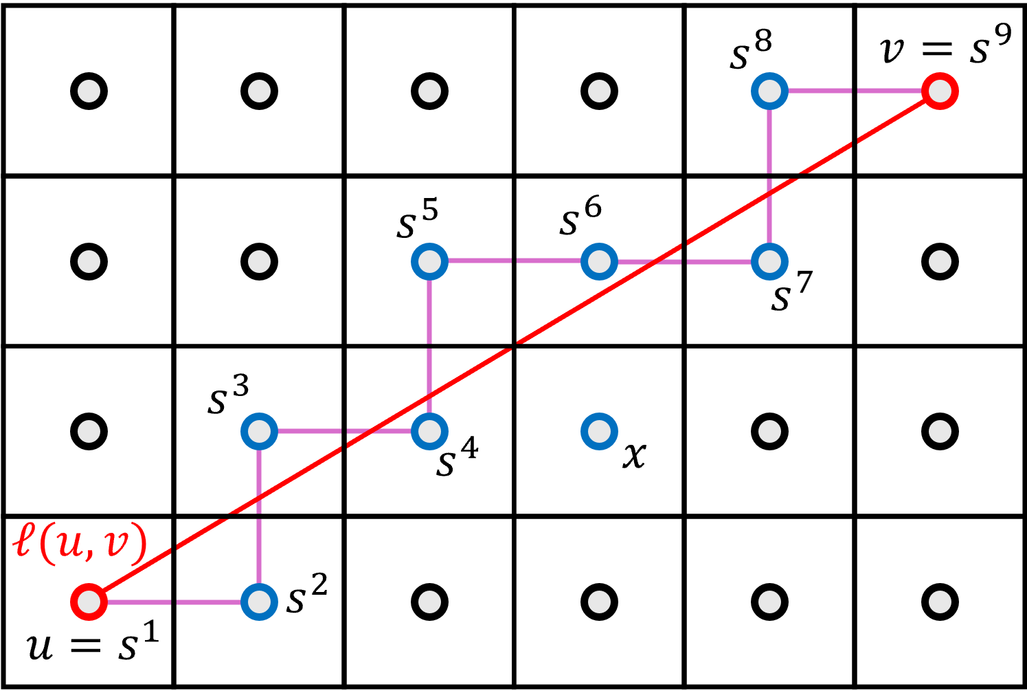
Figure 3: A 2-dimensional example of the construction of Lemma 7, with endpoints $u$ and $v$ and the associated spine vertices $s^{1}$ through $s^{9}$. Each vertex is drawn surrounded by its cube. The vertex $x$ was also an option for $s^{5}$ due to $\ell(u,v)$ passing through a corner of the cubes, but was arbitrarily discarded.

Assume the sequence of vertices $s^{1},\ldots,s^{i-1}$ has been chosen such that (I) and (II) hold for some $m\leq i-1$. We consider three cases:

$(1)$

If $m<i-1$, then we are guaranteed that $s^{m}=v$. Setting $s^{i}=s^{m}$ will satisfy (I) and (II).

$(2)$

If $m=i-1$ and $s^{i-1}=v$, then the construction is finished: we can take $m=i-1$ and $s^{i}=s^{m}$.

$(3)$

Else, let $z_{i-1}=\max\{\mathcal{C}({s^{i-1}})\cap\ell(u,v)\}\,.$ The point $z_{i-1}$ is well-defined by part (II) of the inductive hypothesis.

For each coordinate $j\in[k]$, let $w_{j}=s^{i-1}+\mathbf{e}_{j}$. The face of $\mathcal{C}(s^{i-1})$ with maximum value in coordinate $j$ is shared with the cube $\mathcal{C}(w_{j})$. By Lemma 6, the point $z_{i-1}$ lies on a forward face of $\mathcal{C}({s^{i-1}})$, so there exists $j\in[k]$ such that $z_{i-1}\in\mathcal{C}(w_{j})$. Then choose $s^{i}$ to be the lexicographically smallest point in the set $\{w_{1},\ldots,w_{k}\}$ with the property that $z_{i-1}\in\mathcal{C}(s^{i})$.

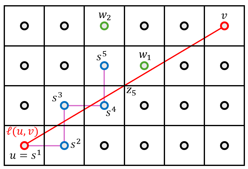
Figure 4: The example from Figure 3, where so far only $\mathbf{s}=(s^{1},\ldots,s^{5})$ has been selected. In the next iteration ($i=6$), we need to choose $s^{6}$. Since $v\not\in\mathbf{s}$, it must be the case that $m=5$. Then we are in case (3), which defines a point $z_{5}=\max\{\mathcal{C}({s^{5}})\cap\ell(u,v)\}$, and two candidates $w_{1}$ and $w_{2}$ for $s^{6}$. Of these two candidates, only $w_{1}$ has the property that $z_{5}\in\mathcal{C}(w_{1})$, so we must choose $s^{6}=w_{1}$.

We show that (I) and (II) continue to hold. Since $(s^{1},\ldots,s^{i-1})$ is a monotone connected path and $s^{i}=s^{i-1}+\mathbf{e}_{j}$ for some $j\in[k]$, the whole path $(s^{1},\ldots,s^{i})$ is also monotone and connected. Thus (I) holds. Also, $z_{i-1}\in\mathcal{C}(s^{i})$, so (II) holds, completing the induction step.

What remains is showing that this construction eventually triggers the $s^{m}=v$ case. The line segment $\ell(u,v)$ is finite, so it can be enclosed by some finite hypercube. However, because $s^{1},s^{2},\ldots$ is a strictly increasing monotone sequence in $\{0,\ldots,n-1\}^{k}$, it will eventually leave any bounded region. Since each $s^{i}$ satisfies $\mathcal{C}(s^{i})\cap\ell(u,v)\neq\emptyset$, there can only be finitely many $s^{i}$ before $s^{m}=v$. ∎

See 8

Proof.

By Lemma 4, the value of $f(v)$ depends only on spine vertices with coordinates each within $2L$ of $v$. In particular, this only includes vertices with Hamming weight within $2kL$ of $wt(v)$. Because $\rho>2kL$, all such vertices are in one of $R_{\alpha-\rho}$, $R_{\alpha}$, and $R_{\alpha+\rho}$ – up to one region away from $v$.

These spine vertices in turn are defined by the spine’s endpoints in the boundaries of $R_{\alpha-\rho}$, $R_{\alpha}$, and $R_{\alpha+\rho}$; specifically, the spine’s intersection with $Low_{\alpha+i\rho}$, for $i\in\{-1,\ldots,2\}$. By the construction of $\mathcal{U}$, the spine’s intersections with all further boundaries are independent of these. Therefore, the spine in regions $R_{\alpha-\rho}$ through $R_{\alpha+\rho}$ is independent of the spine in any region $R_{\alpha+i\rho}$ for $i<-2$ or $i>2$, which completes the proof. ∎

Appendix C Proof of the Main Theorem

This section includes the proofs of lemmas from Section 5.

See 9

Proof.

For all $x_{1},\ldots,x_{\lfloor k/2\rfloor}\in\{-L,\ldots,L\}$, define

$$g(x_{1},\ldots,x_{\lfloor k/2\rfloor})=\begin{cases}\left(\frac{a}{k}+x_{1},\frac{a}{k}-x_{1},\frac{a}{k}+x_{2},\frac{a}{k}-x_{2},\ldots,\frac{a}{k}+x_{\lfloor\frac{k}{2}\rfloor},\frac{a}{k}-x_{\lfloor\frac{k}{2}\rfloor}\right)&\text{if $k$ is even}\\ \left(\frac{a}{k}+x_{1},\frac{a}{k}-x_{1},\frac{a}{k}+x_{2},\frac{a}{k}-x_{2},\ldots,\frac{a}{k}+x_{\lfloor\frac{k}{2}\rfloor},\frac{a}{k}-x_{\lfloor\frac{k}{2}\rfloor},\frac{a}{k}\right)&\text{if $k$ is odd}\end{cases}$$ (43)

We show that $g(x_{1},\ldots,x_{\lfloor\frac{k}{2}\rfloor})\in Low_{a}$ by arguing that $g(x_{1},\ldots,x_{\lfloor\frac{k}{2}\rfloor})\in T_{L}$ and its Hamming weight is $a$.

We first argue that $g(x_{1},\ldots,x_{\lfloor\frac{k}{2}\rfloor})\in\{0,\ldots,n-1\}^{k}$. Let $i=a/k$. Since $a\in\mathcal{I}$, we have $k\mid a$, so $i\in\mathbb{N}$ and $g(x_{1},\ldots,x_{\lfloor\frac{k}{2}\rfloor})\in\mathbb{Z}^{k}$. Because $a\in\mathcal{I}\setminus\{0,k(n-1)\}$, by definition of $\mathcal{I}$ it must be the case that $a\in[\rho,k(n-1)-\rho]$, so:

$$\frac{a}{k}\geq\frac{\rho}{k}\geq 12L\qquad\mbox{and}\qquad\frac{a}{k}\leq\frac{k(n-1)-\rho}{k}\leq(n-1)-12L\,.$$ (44)

Therefore adding terms of magnitude at most $L$ to each coordinate of $(i,\ldots,i)$ leaves $g(x_{1},\ldots,x_{\lfloor\frac{k}{2}\rfloor})$ in $\{0,\ldots,n-1\}^{k}$.

We now argue that $g(x_{1},\ldots,x_{\lfloor\frac{k}{2}\rfloor})\in T_{L}$ because each of its components is within $L$ of $i$. For each $j\in\{1,\ldots,\lfloor k/2\rfloor\}$, we have

$$\left|\frac{a}{k}+x_{j}-i\right|=|x_{j}|\leq L\qquad\mbox{and}\qquad\left|\frac{a}{k}-x_{j}-i\right|=|x_{j}|\leq L\,.$$ (45)

Thus the condition (2) from the definition of the tube holds, so $g(x_{1},\ldots,x_{\lfloor\frac{k}{2}\rfloor})\in T_{L}$.

We have that it has Hamming weight $a$ because each of the $x_{j}$’s cancel out when adding up the coordinates. Therefore, $g(x_{1},\ldots,x_{\lfloor\frac{k}{2}\rfloor})\in Low_{a}$.

As different values of the $x_{j}$’s result in different values of their corresponding coordinates, each choice of $x_{1},\ldots,x_{\lfloor\frac{k}{2}\rfloor}\in\{-L,\ldots,L\}$ yields a distinct point. Thus $|Low_{a}|\geq(2L+1)^{\lfloor k/2\rfloor}$ as required. ∎

See 10

Proof.

For each $u\in Low_{a}$, we have $wt(u)=a$. Similarly, for each $v\in Low_{b}$, we have $wt(v)=b$. Lemma 7 gives a monotone path $\mathbf{s}(u,v)=(s^{1},\ldots,s^{m})$ from $u$ to $v$, so each vertex $s^{i}$ on the path satisfies $a\leq wt(s^{i})\leq b$. If $wt(w)<a$ or $wt(w)>b$, then $w$ cannot be one of the vertices $s^{i}$, so $Pr\bigl{[}w\in\mathbf{s}(U,V)\bigr{]}=0$, thus inequality (6) holds.

Thus from now we can assume $wt(w)\in[a,b]$. Without loss of generality, we assume $w$ lies closer to $Low_{b}$ than $Low_{a}$, i.e.:

$$wt(w)\geq\frac{a+b}{2}\,.$$ (46)

Fix an arbitrary vertex ${u}\in Low_{a}$. Let $B$ denote the hyperplane:

$$B=\{\mathbf{x}\in\mathbb{R}^{k}\mid x_{1}+\ldots+x_{k}=b\}$$ (47)

Let $\mathcal{P}(w)$ denote the projection of $\mathcal{C}(w)$ onto $B$ from $u$, i.e.:

$$\mathcal{P}(w)=\{\mathbf{x}\in B\mid\mathcal{C}(w)\cap\ell(u,\mathbf{x})\neq\emptyset\},$$ (48)

recalling that $\mathcal{C}(w)$ is the cube of side-length $1$ centered at $w$.

By construction, $\mathbf{s}(u,V)$ consists only of vertices $x\in\{0,\ldots,n-1\}^{k}$ for which $\mathcal{C}(x)$ intersects the line segment $\ell(u,V)$ from $u$ to $V$. Then $w\in\mathbf{s}(u,V)$ only if $V\in\mathcal{P}(w)$.

To bound the number of lattice points in $\mathcal{P}(w)$, we will upper-bound the distance between any two points in $\mathcal{P}(w)$. Consider two arbitrary points $p,q\in\mathcal{P}(w)$. Arbitrarily choose $\overline{p}\in\mathcal{C}(w)\cap\ell(u,p)$ and $\overline{q}\in\mathcal{C}(w)\cap\ell(u,q)$.

We claim that $\overline{p}\neq u$ and show it by arguing the two points have very different Hamming weight. Consider an arbitrary $x\in\mathcal{C}(w)$. Since $\|x-w\|_{\infty}\leq 1/2$, we have

$$wt(x) \geq wt(w)-\frac{1}{2}\cdot k\,.$$ (49)

Then

$$wt(x)-wt(u) \geq wt(w)-\frac{1}{2}\cdot k-wt(u)$$ (By (49))

$$\geq\frac{a+b}{2}-\frac{k}{2}-a=\frac{b-a}{2}-\frac{k}{2}$$ (By (46))

$$\geq\frac{b-a}{2}-\frac{b-a}{24L}$$

$$\geq\frac{11}{24}(b-a)\,.$$ (50)

Inequality (50) implies that $x\neq u$. In particular, we have $wt(\overline{p})>wt(u)$ since $\overline{p}\in\mathcal{C}(w)$ and $b-a>0$.

Then define

$$\widetilde{q}=u+(\overline{q}-u)\frac{wt(p-u)}{wt(\overline{p}-u)}\,.$$ (51)

That is, $\widetilde{q}$ is the point that $\overline{q}$ would map to if $\mathcal{C}(w)$ were proportionally scaled from $u$ by the factor required to map $\overline{p}$ to $p$.

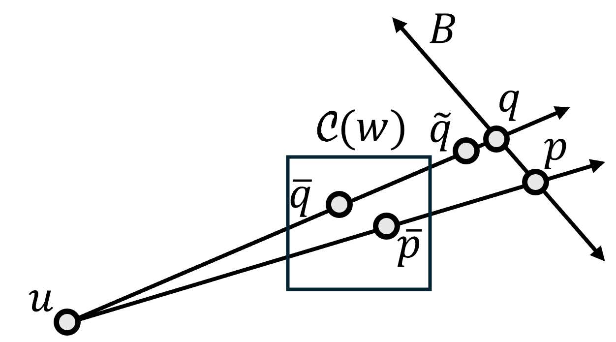
Figure 5: The geometry of Lemma 10, including only what is defined through equation (51). The point $u\in Low_{a}$ is arbitrary. Points $p$ and $q$ lie on the plane $B$ that contains $Low_{b}$ such that $\mathcal{C}(w)$ (for a vertex $w$ not pictured) lies between them and $u$. Lines from $u$ to each of $p$ and $q$ are also drawn, with points $\overline{p}$ and $\overline{q}$ being arbitrary points within $\mathcal{C}(w)$ and each of these lines. Point $\widetilde{q}$ is chosen so that triangles $\overline{q}u\overline{p}$ and $\widetilde{q}up$ are similar.

Since $\overline{p},\overline{q}\in\mathcal{C}(w)$, which is a hypercube of side length $1$, we have:

$$\|\overline{p}-\overline{q}\|_{\infty}\leq 1\,.$$ (52)

We now argue that (52) implies a similar inequality on $\|p-\widetilde{q}\|_{\infty}$. Let $\mathbbm{1}=(1,\ldots,1)$ and let $\theta$ be the angle between $\mathbbm{1}$ and $(p-u)$; since $(p-u)$ and $(\overline{p}-u)$ are parallel, this is also the angle between $(\overline{p}-u)$ and $\mathbbm{1}$. Because $(p-u)$ is parallel to $(\overline{p}-u)$:

$$p =u+(p-u)$$ (53)

$$=u+(\overline{p}-u)\frac{\|p-u\|_{2}\|\mathbbm{1}\|_{2}\cos\theta}{\|\overline{p}-u\|_{2}\|\mathbbm{1}\|_{2}\cos\theta} (p-u) (\overline{p}-u)$$ (Since is parallel to )

$$=u+(\overline{p}-u)\frac{\langle p-u,\mathbbm{1}\rangle}{\langle\overline{p}-u,\mathbbm{1}\rangle}$$ (54)

$$=u+(\overline{p}-u)\frac{wt(p-u)}{wt(\overline{p}-u)}$$ (55)

Combining (51) and (55) gives:

$$\|p-\widetilde{q}\|_{\infty} =\left\|(\overline{p}-\overline{q})\frac{wt(p-u)}{wt(\overline{p}-u)}\right\|_{\infty}=\|\overline{p}-\overline{q}\|_{\infty}\frac{wt(p-u)}{wt(\overline{p}-u)}$$

$$=\|\overline{p}-\overline{q}\|_{\infty}\frac{b-a}{wt(\overline{p}-u)} p\in B wt(p)=b u\in Low_{a} wt(u)=a$$ (Since , so , and , so )

$$\leq 1\cdot\frac{b-a}{\left(\frac{11}{24}(b-a)\right)} x=\overline{p}$$ (By (50) applied to and (52))

$$=\frac{24}{11}\,.$$ (56)

We now show that $\|q-\widetilde{q}\|_{\infty}$ is small. Intuitively, since $p\in B$, by (56) we have that $\widetilde{q}$ is close to $B$; also since $q\in B$ and $q$ is collinear with $\widetilde{q}$ and $u$, they must be close to each other. To formally show this, consider $(\overline{q}-u)$, which is parallel to $(q-\widetilde{q})$. We define $\overline{B}$ as the plane parallel to $B$ through $\overline{q}$:

$$\overline{B}=\Bigl{\{}\mathbf{x}\in\mathbb{R}^{k}\mid x_{1}+\ldots+x_{k}=wt(\overline{q})\Bigr{\}}\,.$$ (57)

Let $z$ be the projection of $u$ onto $\overline{B}$ in the direction $\mathbbm{1}$.

We have:

$$wt(z)-wt(u) =wt(\overline{q})-wt(u) z\in\overline{B}$$ (Because )

$$\geq\frac{11}{24}(b-a) \overline{q}$$ (By applying (50) to .)

Since $z-u$ has slope $(1,\ldots,1)$ by definition of $z$, the coordinates of $z-u$ are all the same. Therefore for all $i\in[k]$:

$$(z-u)_{i} \geq\frac{11}{24k}(b-a)$$ (Using (LABEL:eq:wt_z_minus_wt_u_lb))

$$\geq\frac{11}{2}L$$ (59)

Define the continuous version $T^{C}_{L}$ of the tube $T_{L}$ as:

$$T^{C}_{L}=\Bigl{\{}\mathbf{x}\in\mathbb{R}^{k}\mid\exists\alpha\in\mathbb{R}\mbox{ such that }|x_{j}-\alpha|\leq L\ \forall j\in[k]\Bigr{\}}$$ (60)

Let $\mathbf{y}\in T_{L}^{C}\cap\overline{B}$ be arbitrary, and let $\alpha_{y}$ be its value of $\alpha$ from (60). Because $\mathbf{y}\in\overline{B}$, we have the pair of inequalities:

$$wt(\overline{q}) =\sum_{i=1}^{k}y_{i}\leq k(\alpha_{y}+L)$$ (61)

$$wt(\overline{q}) =\sum_{i=1}^{k}y_{i}\geq k(\alpha_{y}-L)$$ (62)

Solving each of (62) and (61) for $\alpha_{y}$ gives $|\alpha_{y}-(wt(\overline{q})/k)|\leq L$. As $\mathbf{y}\in T_{L}^{C}\cap\overline{B}$ was arbitrary, this bound applies to the corresponding values $\alpha_{\overline{q}}$ and $\alpha_{z}$ for $\overline{q}$ and $z$:

$$\left|\alpha_{\overline{q}}-\frac{wt(\overline{q})}{k}\right| \leq L$$ (63)

$$\left|\alpha_{z}-\frac{wt(\overline{q})}{k}\right| \leq L$$ (64)

We now get:

$$\|\overline{q}-z\|_{\infty} \leq(\max(\alpha_{\overline{q}},\alpha_{z})+L)-(\min(\alpha_{\overline{q}},\alpha_{z})-L) \overline{q},z\in T^{C}_{L}$$ (As )

$$=|\alpha_{\overline{q}}-\alpha_{z}|+2L$$ (65)

$$\leq L+L+2L$$ (By the triangle inequality with (63) and (64))

$$=4L$$ (66)

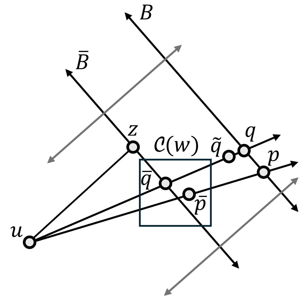
Figure 6: The geometry of Lemma 10. In addition to what is pictured in Figure 5, this diagram includes the plane $\overline{B}$, which is parallel to $B$ and goes through $\overline{q}$. The point $z\in\overline{B}$ is such that the segment $uz$ is perpendicular to $\overline{B}$. The unlabeled lighter lines in the top-left and bottom-right represent the edges of the tube $T_{L}$.

Since all the components of $z-u$ are the same, we have

$$\max_{i,j\in[k]}\frac{(\overline{q}-u)_{i}}{(\overline{q}-u)_{j}}=\max_{i,j\in[k]}\frac{(\overline{q}-z)_{i}+(z-u)_{i}}{(\overline{q}-z)_{j}+(z-u)_{j}}=\max_{i,j\in[k]}\frac{(\overline{q}-z)_{i}+(z-u)_{i}}{(\overline{q}-z)_{j}+(z-u)_{i}}$$ (67)

Inequality (59) gives $(z-u)_{i}\geq\frac{11}{2}L$, so

$$-4L+(z-u)_{i}>0\,.$$ (68)

We obtain

$$\max_{i,j\in[k]}\frac{(\overline{q}-z)_{i}+(z-u)_{i}}{(\overline{q}-z)_{j}+(z-u)_{i}} \leq\max_{i,j\in[k]}\frac{4L+(z-u)_{i}}{-4L+(z-u)_{i}}$$ (By (66) and (68))

$$\leq\frac{\frac{11}{2}L+4L}{\frac{11}{2}L-4L}$$ (By (59))

$$=\frac{19}{3}\,.$$ (69)

Combining (67) and (69) yields

$$\max_{i,j\in[k]}\frac{(\overline{q}-u)_{i}}{(\overline{q}-u)_{j}}\leq\frac{19}{3}\,.$$ (70)

Because $\overline{q}-u$ and $q-\widetilde{q}$ are parallel, we have $(q-\widetilde{q})=\beta(\overline{q}-u)$ for some $\beta\in\mathbb{R}$. Therefore applying (70) gives

$$\max_{i,j\in[k]}\frac{(q-\widetilde{q})_{i}}{(q-\widetilde{q})_{j}}=\max_{i,j\in[k]}\frac{\beta(\overline{q}-u)_{i}}{\beta(\overline{q}-u)_{j}}\leq\frac{19}{3}\,.$$ (71)

We also have

$$|wt(\widetilde{q})-b| =\left|\sum_{i=1}^{k}\widetilde{q}_{i}-p_{i}\right| p\in B \sum_{i=1}^{k}p_{i}=b$$ (Since , we have )

$$\leq\sum_{i=1}^{k}\left|\widetilde{q}_{i}-p_{i}\right|$$ (By triangle inequality)

$$\leq\frac{24}{11}k\,. \|p-\widetilde{q}\|_{\infty}\leq 24/11$$ (Since by (56))

We define the unit-weight vector in the direction of $q-\widetilde{q}$ as

$$d=\frac{q-\widetilde{q}}{wt(q-\widetilde{q})}\,.$$ (73)

We then have:

$$\max_{i\in[k]}d_{i} =\left(\min_{j\in[k]}d_{j}\right)\cdot\left(\max_{i,j\in[k]}\frac{d_{i}}{d_{j}}\right)$$ (74)

$$\leq\frac{1}{k}\cdot\left(\max_{i,j\in[k]}\frac{d_{i}}{d_{j}}\right)$$ (75)

$$\leq\frac{19}{3k} d q-\widetilde{q}$$ (Since is parallel to , so the bound of (71) applies)

Therefore:

$$\|q-\widetilde{q}\|_{\infty} =\|d\|_{\infty}\cdot|wt(\tilde{q})-b|$$ (77)

$$\leq\frac{19}{3k}\cdot\frac{24}{11}k$$ (By (LABEL:eq:9_over_k_bound) and (LABEL:eq:up_wt_q_tilde_minus_b_absolute))

$$=\frac{152}{11}\,.$$ (78)

Inequality (56) gives $\|p-\widetilde{q}\|_{\infty}\leq 24/11$. Since $\|q-\widetilde{q}\|_{\infty}\leq 152/11$ by (78), applying the triangle inequality gives

$$\|p-q\|_{\infty}\leq\|p-\widetilde{q}\|_{\infty}+\|q-\widetilde{q}\|_{\infty}\leq\frac{24}{11}+\frac{152}{11}=16\,.$$ (79)

Since this bound applies to any two points $p,q\in\mathcal{P}(w)$, all of $\mathcal{P}(w)$ fits inside a hypercube of side length $16$. This hypercube contains at most $(16+1)^{k}$ lattice points, so at most $17^{k}$ realizations of $V$ could result in $\mathbf{s}(u,V)$ passing through $w$. Since the total number of realizations of $V$ is $|Low_{b}|$, we have

$$\Pr\Bigl{[}w\in\mathbf{s}(u,V)\Bigr{]} \leq\frac{17^{k}}{|Low_{b}|}$$ (80)

$$\leq\frac{17^{k}}{(2L+1)^{\lfloor k/2\rfloor}}\,.$$ (By Lemma 9)

This bound applies to any fixed $u\in Low_{a}$, so it also holds when $u$ is chosen uniformly at random from $Low_{a}$. Thus for $U\sim\mathcal{U}(Low_{a})$ and $V\sim\mathcal{U}(Low_{b})$ we have

$$\Pr\Bigl{[}w\in\mathbf{s}(U,V)\Bigr{]} \leq\frac{17^{k}}{(2L+1)^{\lfloor k/2\rfloor}},$$ (81)

as required. ∎

Lemma 15.

Let $X_{1},\ldots,X_{m}$ be nonnegative, possibly correlated random variables. Let $C\in\mathbb{R}$ be such that $\mathbb{E}[X_{i}]\leq C$ for all $i\in[m]$. Then:

$$\mathbb{E}\left[\max_{i\in[m]}X_{i}\right] \leq mC\,.$$ (82)

Proof.

Because the $X_{i}$ are nonnegative, their maximum is at most their sum. Therefore:

$$\mathbb{E}\left[\max_{i\in[m]}X_{i}\right] \leq\mathbb{E}\left[\sum_{i=1}^{m}X_{i}\right]=\sum_{i=1}^{m}\mathbb{E}[X_{i}]\leq mC\,.$$ (83)

∎

See 11

Proof.

Consider the roles $v$ might play for an arbitrary spine $\mathbf{s}$ and index $j$:

• If $v$ is the fixed point of $h^{\mathbf{s},j}$, then $h^{\mathbf{s},j}(v)=v$.

• If $v$ is on the spine $\mathbf{s}$ but is not the fixed point, then $h^{\mathbf{s},j}(v)$ differs from $v$ in exactly one coordinate, and is either one more or one less in that coordinate. There are $2k$ ways to choose such a value.

• If $v$ is not on the spine $\mathbf{s}$, then $h^{\mathbf{s},j}(v)$ differs from $v$ in exactly two coordinates: one in which $h^{\mathbf{s},j}$ is one bigger, and one in which it is one smaller. There are $k(k-1)$ ways to choose such a value.

Therefore:

$$|F(v)| \leq 1+2k+k(k-1)=k^{2}+k+1\leq k^{3},$$ (84)

which completes the proof. ∎

See 12

Proof.

In this proof, all probabilities and expectations are taken over the input function $f\sim\mathcal{U}$.

For each region $R$, define the following random variables:

• $P_{t}(R)=\max_{v\in R}\log_{2}\Pr\left[\text{$v$ is a spine vertex after $t$ queries from $\mathcal{A}$}\right]$.

• $P^{*}_{t}(R)=\max_{0\leq t^{*}\leq t}P_{t^{*}}(R)$.

Define the set:

$$G_{m}=\left\{(R^{1},\ldots,R^{m})\mid R^{1},\ldots,R^{m}\mbox{ are regions, }dist(R^{i},R^{j})\geq 5\mbox{ for all }i\neq j\in[m]\right\}\,.$$ (85)

That is, $G_{m}$ is the set of $m$-tuples of regions which $\mathcal{A}$ is trying to find spine vertices in. Finally, let:

$$\overline{P}_{t} =\max_{(R^{1},\ldots,R^{m})\in G_{m}}\sum_{i=1}^{m}P^{*}_{t}(R^{i})\,.$$ (86)

We aim to upper-bound $\mathbb{E}[\overline{P}_{t+1}-\overline{P}_{t}]$. To do so, we condition on the history $\mathcal{H}_{t}$ of the first $t$ queries made by $\mathcal{A}$ and their responses.

As in Lemma 11, for each vertex $v$, let $F(v)$ be the set of possible responses to querying $v$:

$$F(v) =\left\{y\in\{0,\ldots,n-1\}^{k}\mid\exists\mathbf{s}\in\Psi,j\in\{0,\ldots,k(n-1)\}\mbox{ such that }h^{\mathbf{s},j}(v)=y\right\}\,.$$

Consider an arbitrary region $R$, and let $q_{t+1}$ be the next query made by $\mathcal{A}$. Let $V_{t}(R)$ be the set of vertices $v\in R$ which could still be spine vertices:

$$V_{t}(R)=\left\{v\in R\mid\Pr[\text{$v$ is a spine vertex}\mid\mathcal{H}_{t}]>0\right\}\,.$$ (87)

We now upper-bound $\mathbb{E}[P^{*}_{t+1}(R)-P^{*}_{t}(R)\mid\mathcal{H}_{t}]$. This expectation can be broken into two cases depending on the realizations of $P_{t+1}(R)$ and $P_{t}(R)$:

• If $P_{t+1}(R)>P_{t}(R)$, then $P^{*}_{t+1}(R)-P^{*}_{t}(R)\leq P_{t+1}(R)-P_{t}(R)$.

• If $P_{t+1}(R)\leq P_{t}(R)$, then $P^{*}_{t+1}(R)=P^{*}_{t}(R)$.

In each case, $P^{*}_{t+1}(R)-P^{*}_{t}(R)\leq\max(0,P_{t+1}(R)-P_{t}(R))$. We now decompose that expected value based on the response $a_{t+1}$ to $\mathcal{A}$’s query $q_{t+1}$:

$$\mathbb{E}[P^{*}_{t+1}(R)-P^{*}_{t}(R)\mid\mathcal{H}_{t}]$$ (88)

$$\leq\mathbb{E}[\max(0,P_{t+1}(R)-P_{t}(R))\mid\mathcal{H}_{t}]$$ (89)

$$=\sum_{y\in F(q_{t+1})}\Pr\left[a_{t+1}=y\mid\mathcal{H}_{t}\right]\max\left(0,\log_{2}\left(\frac{\max_{v\in R}\Pr[\text{$v$ is a spine vertex}\mid\mathcal{H}_{t},a_{t+1}=y]}{\max_{w\in R}\Pr[\text{$w$ is a spine vertex}\mid\mathcal{H}_{t}]}\right)\right)$$ (90)

$$\leq\sum_{y\in F(q_{t+1})}\Pr\left[a_{t+1}=y\mid\mathcal{H}_{t}\right]\max\left(0,\max_{v\in V_{t}(R)}\log_{2}\left(\frac{\Pr[\text{$v$ is a spine vertex}\mid\mathcal{H}_{t},a_{t+1}=y]}{\Pr[\text{$v$ is a spine vertex}\mid\mathcal{H}_{t}]}\right)\right)\,.$$ (91)

For arbitrary $v\in R$ and $y\in F(q_{t+1})$, the quantity inside the logarithm in (91) can be upper-bounded by expanding its denominator:

$$\Pr[\text{$v$ is a spine vertex}\mid\mathcal{H}_{t}]$$ (92)

$$=\sum_{w\in F(q_{t+1})}\Pr\left[a_{t+1}=w\mid\mathcal{H}_{t}\right]\cdot\Pr[\text{$v$ is a spine vertex}\mid\mathcal{H}_{t},a_{t+1}=w]$$ (93)

$$\geq\Pr\left[a_{t+1}=y\mid\mathcal{H}_{t}\right]\cdot\Pr[\text{$v$ is a spine vertex}\mid\mathcal{H}_{t},a_{t+1}=y]\,.$$ (94)

Dividing both sides of (94) by $\Pr[\text{$v$ is a spine vertex}\mid\mathcal{H}_{t}]$ and $\Pr\left[a_{t+1}=y\mid\mathcal{H}_{t}\right]$ gives:

$$\frac{\Pr[\text{$v$ is a spine vertex}\mid\mathcal{H}_{t},a_{t+1}=y]}{\Pr[\text{$v$ is a spine vertex}\mid\mathcal{H}_{t}]}\leq\frac{1}{\Pr\left[a_{t+1}=y\mid\mathcal{H}_{t}\right]}\,.$$ (95)

Applying (95) to (91) gives:

$$\mathbb{E}[P^{*}_{t+1}(R)-P^{*}_{t}(R)\mid\mathcal{H}_{t}]$$ (96)

$$\leq\sum_{y\in F(q_{t+1})}\Pr\left[a_{t+1}=y\mid\mathcal{H}_{t}\right]\max\left(0,\max_{v\in V_{t}(R)}\log_{2}\left(\frac{1}{\Pr\left[a_{t+1}=y\mid\mathcal{H}_{t}\right]}\right)\right)$$ (97)

$$=\sum_{y\in F(q_{t+1})}-\Pr\left[a_{t+1}=y\mid\mathcal{H}_{t}\right]\min\left(0,\log_{2}\Pr\left[a_{t+1}=y\mid\mathcal{H}_{t}\right]\right)$$ (98)

$$\leq\sum_{y\in F(q_{t+1})}-\Pr\left[a_{t+1}=y\mid\mathcal{H}_{t}\right]\log_{2}\Pr\left[a_{t+1}=y\mid\mathcal{H}_{t}\right]\,.$$ (99)

Because (99) is precisely the entropy of $a_{t+1}$ given $\mathcal{H}_{t}$, it can be upper-bounded by the entropy of a uniform distribution over $F(q_{t+1})$. Further applying Lemma 11:

$$\mathbb{E}[P^{*}_{t+1}(R)-P^{*}_{t}(R)\mid\mathcal{H}_{t}] \leq\log_{2}(|F(q_{t+1})|)\leq 3\log_{2}(k)$$ (100)

We now bound $\mathbb{E}[\overline{P}_{t+1}-\overline{P}_{t}\mid\mathcal{H}_{t}]$. This gain is upper-bounded by the expected “most improved” tuple in $G_{m}$:

$$\mathbb{E}[\overline{P}_{t+1}-\overline{P}_{t}\mid\mathcal{H}_{t}] \leq\mathbb{E}\left[\max_{(R^{1},\ldots,R^{m})\in G_{m}}\sum_{i=1}^{m}P^{*}_{t+1}(R^{i})-P^{*}_{t}(R^{i})\mid\mathcal{H}_{t}\right]\,.$$ (101)

Each tuple in $G_{m}$ contains only regions that are at least five apart. By Lemma 8, querying $q_{t+1}$ can only update knowledge about the spine in a block of five consecutive regions; call this block $U(q_{t+1})$. Therefore, each individual sum in (101) contains at most one nonzero term, and all such terms are for one of the five regions in $U(q_{t+1})$. Therefore:

$$\mathbb{E}[\overline{P}_{t+1}-\overline{P}_{t}\mid\mathcal{H}_{t}] \leq\mathbb{E}\left[\max_{R\in U(q_{t+1})}P^{*}_{t+1}(R)-P^{*}_{t}(R)\mid\mathcal{H}_{t}\right]\,.$$ (102)

Because $P^{*}_{t+1}(R)-P^{*}_{t}(R)\geq 0$ for all regions $R$, Lemma 15 combined with (100) applies to give:

$$\mathbb{E}[\overline{P}_{t+1}-\overline{P}_{t}\mid\mathcal{H}_{t}] \leq 15\log_{2}(k)\,.$$ (103)

And as the upper bound in (103) applies independently of $\mathcal{H}_{t}$, taking the expectation over $\mathcal{H}_{t}$ gives the history-independent bound:

$$\mathbb{E}[\overline{P}_{t+1}-\overline{P}_{t}] \leq 15\log_{2}(k)\,.$$ (104)

Now suppose an algorithm $\mathcal{A}$ makes at most $T$ queries. By telescoping (104), we get:

$$\mathbb{E}[\overline{P}_{T}-\overline{P}_{0}] \leq 15T\log_{2}(k)\,.$$ (105)

When $\mathcal{A}$ succeeds, it has found $m$ spine vertices in regions at least five apart, and therefore $\overline{P}_{T}=0$. By Lemma 10, no vertex other than those in regions $R_{0}$ and $R_{k(n-1)-\rho}$ initially has a chance higher than $17^{k}/(2L+1)^{\lfloor k/2\rfloor}$ to be on the spine. In those regions, we can vacuously upper-bound $P^{*}_{0}(R_{0})$ and $P^{*}_{0}(R_{k(n-1)-\rho})$ by $0$, so:

$$\overline{P}_{0} \leq(m-2)\log_{2}\left(\frac{17^{k}}{(2L+1)^{\lfloor k/2\rfloor}}\right)\,.$$ (106)

Therefore, by Markov’s inequality, the probability $\mathcal{A}$ succeeds within $T$ queries is at most:

$$\Pr[\text{$\mathcal{A}$ succeeds in $T$ queries}] \leq\frac{15T\log_{2}(k)}{(m-2)\cdot\left(\lfloor k/2\rfloor\log_{2}(2L+1)-k\log_{2}(17)\right)}\,.$$ (107)

This completes the proof. ∎

We now present Lemma 13, which states that solving $TARSKI(n,k)$ requires querying spine vertices in many different regions. Its proof is based around the classical ordered search problem:

Definition 11 (Ordered search).

The input is a bit vector $\mathbf{x}=(x_{1},\ldots,x_{m})\in\{0,1\}^{m}$ with the promise that exactly one bit is set to $1$. The vector can be accessed via oracle queries of the form: “Is the $i$-th bit equal to $1$?”. The answer to a query is: “Yes”, “No, go left”, or “No, go right”. The task is to find the location of the hidden bit.

See 13

The proof of Lemma 13 depends on lower bounds for ordered search, which we present afterwards.

Proof.

Whenever $\mathcal{A}$ correctly returns the fixed point, it also learns which region the fixed point is in. We will argue that even learning the region with the fixed point is at least as hard as ordered search on the $m$ regions, where $m=k(n-1)/\rho$.

To that end, let $\mathcal{A}^{\prime}$ be the following randomized algorithm for the ordered search problem of Definition 11, which is given an input $\mathbf{x}\in\{0,1\}^{m}$ with (unknown) answer $j$.

• Draw a spine $\mathbf{t}\in\Psi$ and an offset $\theta\in\{0,\ldots,\rho-1\}$ uniformly at random.

• Set variables $a=0$ and $b=k(n-1)$.

• Simulate $\mathcal{A}$ on $h^{\mathbf{t},\rho j+\theta}$. While $\mathcal{A}^{\prime}$ does not know $j$, it can still answer each query $v$ submitted by $\mathcal{A}$ as follows:

  • If $v\notin\mathbf{t}$, then compute $h^{\mathbf{t},q}(v)$ for an arbitrary $q\in\{0,\ldots,k(n-1)\}$.

  • If $v\in\mathbf{t}$, then let $R_{\rho i}$ be the region containing $v$. Let $\mathcal{A}^{\prime}$ query the vector $\mathbf{x}$ at position $i$; if it had already done so, then look up the result of that query instead. Then:

    • If the response is “No, go left”, then set $b=\min(b,wt(v)-1)$ and give $\mathcal{A}$ the value of $h^{\mathbf{t},q}(v)$ for an arbitrary $q\in[a,b]$.

    • If the response is “No, go right”, then set $a=\max(a,wt(v)+1)$ and give $\mathcal{A}$ the value of $h^{\mathbf{t},q}(v)$ for an arbitrary $q\in[a,b]$.

    • If the response is “Yes”, then halt; the answer has been found.

• Whenever $\mathcal{A}$ outputs $u$ as its answer, $\mathcal{A}^{\prime}$ returns the index $i$ such that $u\in R_{\rho i}$.

We first argue by induction on the number of queries $\mathcal{A}$ makes that:

• $\mathcal{A}^{\prime}$ can accurately simulate $h^{\mathbf{t},\rho j+\theta}$, given its choice of $\mathbf{t}$ and $\theta$.

• $\mathcal{A}^{\prime}$ maintains $\rho j+\theta\in[a,b]$.

The base case is clear, as $\rho j+\theta\geq 0$ and $\rho j+\theta\leq k(n-1)$.

Now suppose that $\rho j+\theta\in[a,b]$ after some number of queries from $\mathcal{A}$. Its next query $v$ falls into one of a few cases:

• $v\notin\mathbf{t}$. Then by definition, the value of $h^{\mathbf{t},\rho j+\theta}(v)$ is independent of $\rho j+\theta$, so $\mathcal{A}^{\prime}$ can compute it.

• $v\in\mathbf{t}$. Then there is a region $R_{\rho i}$ such that $v\in R_{\rho i}$, and $\mathcal{A}^{\prime}$ queries bit $i$ of $\mathbf{x}$. There are three cases for the resulting query:

  • If $\mathcal{A}^{\prime}$ receives “No, go left”, then $i>j$. Therefore, $wt(v)\geq\rho(j+1)$, so after updating $b$ we maintain $b\geq\rho j+\theta$. The value of $h^{\mathbf{t},\rho j+\theta}(v)$ can then be determined from knowing $\mathbf{t}$ and that $wt(v)>\rho j+\theta$.

  • If $\mathcal{A}^{\prime}$ receives “No, go right”, then $i<j$. Therefore, $wt(v)<\rho j$, so after updating $a$ we maintain $a\leq\rho j+\theta$. The value of $h^{\mathbf{t},\rho j+\theta}(v)$ can then be determined from knowing $\mathbf{t}$ and that $wt(v)<\rho j+\theta$.

  • If $\mathcal{A}^{\prime}$ receives “Yes”, then it halts immediately, having found its answer of $j$.

Therefore, by induction, each response $\mathcal{A}$ receives is consistent with $h^{\mathbf{t},\rho j+\theta}$.

If $\mathcal{A}^{\prime}$ is run on an input distribution which is uniformly random over the $m$ possible answers, then its simulated values of both $\mathbf{t}\in\Psi$ and $\rho j+\theta\in\{0,\ldots,k(n-1)\}$ will be uniformly random as well. Therefore, its simulation of $\mathcal{A}$ will be run on inputs from $\mathcal{U}$.

Now suppose $\mathcal{A}$ is correct with probability at least $1-\delta$ on inputs drawn from $\mathcal{U}$. Then $\mathcal{A}^{\prime}$ will be correct with probability at least $1-\delta$ on uniformly random inputs. By Lemma 17, there exists $c=c(\delta,\epsilon)$ such that on this distribution $\mathcal{A}^{\prime}$ makes at least $c\log m$ queries with probability at least $\epsilon$. Because each query $\mathcal{A}^{\prime}$ makes corresponds to a new region queried by $\mathcal{A}$, we have that $\mathcal{A}$ queries at least $c\log m$ regions with probability at least $\epsilon$. ∎

Lemma 16.

Let $\epsilon,\delta\in(0,1)$ such that $\delta+\epsilon<1$. Let $U_{m}$ be the uniform distribution over ordered search instances of length $m$. Let $\mathcal{A}$ be a deterministic algorithm for ordered search with the property that $\Pr_{\mathbf{x}\sim U_{m}}\left[\mathcal{A}\mbox{ succeeds on }\mathbf{x}\right]\geq 1-\delta\,.$ Then there exists $c>0$ such that, for $m>2^{3/(1-\delta-\epsilon)}$:

$$\Pr_{\mathbf{x}\sim U_{m}}\left[\mathcal{A}\mbox{ issues at least }c\log_{2}(m)\mbox{ queries on }\mathbf{x}\right]\geq\epsilon\,.$$ (108)

Proof.

We will use $c=1/6$. For contradiction, suppose $\mathcal{A}$ violated inequality (108). Then consider the following encoding scheme for an integer $z\in[m]$:

• If $\mathcal{A}$ succeeds within $c\log_{2}(m)$ queries on the ordered search instance of length $m$ with answer $z$, then encode $z$ with a $0$ followed by the responses to the queries made by $\mathcal{A}$ on this input. This can be done in $2$ bits per query, for a total of at most $1+2c\log_{2}(m)$ bits.

• Otherwise, encode $z$ with a $1$ followed by its representation in binary. This can be done in $1+\lceil\log_{2}(m)\rceil$ bits.

The probability of the first case occurring on a uniformly random input is at least $1-\delta-\epsilon$, so overall the average number of bits this scheme takes is at most:

$$1+(1-\delta-\epsilon)2c\log_{2}(m)+(\delta+\epsilon)\lceil\log_{2}m\rceil$$ (109)

$$\leq 1+(1-\delta-\epsilon)\frac{1}{3}\log_{2}(m)+(\delta+\epsilon)\log_{2}(m)+1$$ (110)

$$= 2+\frac{2\delta+2\epsilon+1}{3}\log_{2}(m)$$ (111)

$$< \frac{2-2\delta-2\epsilon}{3}\log_{2}(m)+\frac{2\delta+2\epsilon+1}{3}\log_{2}(m) m>2^{3/(1-\delta-\epsilon)}$$ (Because )

$$= \log_{2}(m)\,.$$ (112)

But $\log_{2}(m)$ is the entropy of a uniformly distributed value in $[m]$, so this violates the source coding theorem. Therefore, $\mathcal{A}$ must satisfy (108), which completes the proof. ∎

Lemma 17.

Let $\epsilon,\delta\in(0,1)$ such that $2\delta+2\epsilon<1$. Let $U_{m}$ be the uniform distribution over ordered search instances of length $m$. Let $\mathcal{A}$ be a randomized algorithm for ordered search with the property that

$$\Pr_{\mathbf{x}\sim U_{m}}\left[\mathcal{A}\mbox{ succeeds on }\mathbf{x}\right]\geq 1-\delta\,.$$

Then there exists $c=c(\delta,\epsilon)>0$ such that, for $m>2^{3/(1-2\delta-2\epsilon)}$:

$$\Pr_{\mathbf{x}\sim U_{m}}\left[\mathcal{A}\mbox{ issues at least }c\log(m)\mbox{ queries on }\mathbf{x}\right]\geq\epsilon\,.$$ (113)

Proof.

We can view $\mathcal{A}$ as a distribution $D_{\mathcal{A}}$ over deterministic algorithms. Because the choice of deterministic algorithm occurs before execution, the draw from $D_{\mathcal{A}}$ is independent of the random input. Then by Markov’s inequality:

$$\Pr_{A\sim D_{\mathcal{A}}}\left[\Pr_{\mathbf{x}\sim U_{m}}\left[\text{$A$ fails on $\mathbf{x}$}\right]>2\delta\right] \leq\frac{\mathbb{E}_{A\sim D_{\mathcal{A}}}\left[\Pr_{\mathbf{x}\sim U_{m}}\left[\text{$A$ fails on $\mathbf{x}$}\right]\right]}{2\delta}$$ (114)

$$=\frac{\Pr_{\mathbf{x}\sim U_{m}}\left[\text{$\mathcal{A}$ fails on $\mathbf{x}$}\right]}{2\delta}$$ (115)

$$\leq\frac{1}{2}\,.$$ (116)

We will use the same $c$ as Lemma 16. By that lemma, for any deterministic algorithm $A$ with success probability at least $1-2\delta$ on the uniform distribution:

$$\Pr_{\mathbf{x}\sim U_{m}}\left[A\mbox{ issues at least }c\log_{2}(m)\mbox{ queries on }\mathbf{x}\right]\geq 2\epsilon\,.$$ (117)

Combining (116) and (117):

$$\Pr_{\mathbf{x}\sim U_{m}}\left[\mathcal{A}\mbox{ issues at least }c\log(m)\mbox{ queries on }\mathbf{x}\right]$$ (118)

$$\geq \Pr_{A\sim D_{\mathcal{A}}}\left[\Pr_{\mathbf{x}\sim U_{m}}\left[\text{$A$ succeeds on $\mathbf{x}$}\right]\geq 1-2\delta\right]$$ (119)

$$\cdot\mathbb{E}_{A\sim D_{\mathcal{A}}}\left[\Pr_{\mathbf{x}\sim U_{m}}\left[A\mbox{ issues at least }c\log(m)\mbox{ queries on }\mathbf{x}\right]\mid\Pr_{\mathbf{x}\sim U_{m}}\left[\text{$A$ succeeds on $\mathbf{x}$}\right]\geq 1-2\delta\right]$$

$$\geq \frac{1}{2}\cdot 2\epsilon$$ (120)

$$= \epsilon\,.$$ (121)

This completes the proof. ∎

Appendix D An $O(k\log n\log(nk))$ upper bound for multi-dimensional herring-bone functions

In this section we include the proofs of statements in Section 6.

See 2

Proof.

By Lemma 18, the spine vertex with any particular Hamming weight can be found in $O(k\log n)$ queries. This subroutine can be used to run binary search to locate the fixed point along the spine.

Specifically, suppose the (unknown) instance is $h^{\mathbf{s},j}$ for some $\mathbf{s}\in\Psi$ and $j\in\{0,\ldots,(n-1)k\}$. For an arbitrary $x\in\{0,\ldots,(n-1)k\}$, querying the spine vertex $s^{x}$ produce three different options depending on how $x$ compares to $j$:

• If $x=j$, then $h^{\mathbf{s},j}(s^{x})=s^{x}$. This is the fixed point.

• If $x<j$, then $h^{\mathbf{s},j}(s^{x})=s^{x+1}$. This is identifiable because $h^{\mathbf{s},j}(s^{x})>s^{x}$ only in this case.

• If $x>j$, then $h^{\mathbf{s},j}(s^{x})=s^{x-1}$. This is identifiable because $h^{\mathbf{s},j}(s^{x})<s^{x}$ only in this case.

This is enough feedback to run binary search to find $j$. Binary search takes $O(\log(nk))$ iterations to identify $j\in\{0,\ldots,(n-1)k\}$, so overall this algorithm uses $O(k\log(n)\log(nk))$ queries. ∎

Lemma 18.

Given a value $0\leq x\leq(n-1)k$, there is an $O(k\log(n))$-query algorithm to find the spine vertex $s^{x}=(s^{x}_{1},\ldots,s^{x}_{k})$ that is Hamming distance $x$ from the origin in a multi-dimensional herringbone function.

Proof.

Let $a^{1}_{i}=0$, let $b^{1}_{i}=x/k$, and let $c^{1}_{i}=n-1$ for all $i\in[k]$. We then perform the following steps repeatedly until a spine vertex is returned. Let the iteration number be $m$, starting with $1$. We use the notation $a^{m}=(a^{m}_{1},\ldots,a^{m}_{k})$ for all vertices $a^{m}$.

1. Query $f(b^{m})$.

2. If $\|f(b^{m})-b^{m}\|\leq 1$, return $b^{m}$ since it must be a spine vertex.

3. Otherwise, there are dimensions $p,q\in[k]$ such that $(f(b^{m}))_{p}-b^{m}_{p}=b^{m}_{q}-(f(b^{m}))_{q}=1$.

4. Set $a^{m+1}=a^{m}$ and $c^{m+1}=c^{m}$, except for $a^{m+1}_{p}$, which we set equal to $b^{m}_{p}$ and $c^{m+1}_{q}$ which we set equal to $b^{m}_{q}$.

5. Let $d^{m}=\min(c^{m}_{p}-b^{m}_{p},b^{m}_{q}-a^{m}_{q})$. Set $b^{m+1}=b^{m}$, except for $b^{m+1}_{p}$ which we set equal to $b^{m}_{p}+d^{m}/2$ and $b^{m+1}_{q}$ which we set equal to $b^{m}_{q}-d^{m}/2$.

We claim the above algorithm maintains the following invariants for all $m$:

1. $a^{m}\leq b^{m}\leq c^{m}$.

2. $a^{m}\leq s^{x}\leq c^{m}$.

3. $b^{m}$ is Hamming distance $x$ from the origin.

The invariants are initially true by the initialization of $a^{1},b^{1},c^{1}$. Suppose inductively that the invariants hold for $a^{m},b^{m},c^{m}$. We will show they hold for $a^{m+1},b^{m+1},c^{m+1}$ if the algorithm did not return in or before iteration $m$.

Assuming the algorithm did not return in iteration $m$, we have dimensions $p,q$ such that $(f(b^{m}))_{p}-b^{m}_{p}=b^{m}_{q}-(f(b^{m}))_{q}=1$. Then $b^{m}_{p}=s^{\mu(b^{m})}_{p}$. Furthermore, $s^{x}\geq s^{\mu(b^{m})}$ since all spine vertices are fully ordered and $s^{\mu(b^{m})}$ has Hamming distance from the origin strictly less than $x$. Therefore $s^{x}_{p}\geq b^{m}_{p}$, so $a^{m+1}_{p}\leq s^{x}_{p}$ as required. By symmetric logic, $s^{x}_{q}\leq c^{m+1}_{q}$. All other components of $a^{m+1}\leq s^{x}\leq c^{m+1}$ hold since $a^{m}\leq s^{x}\leq c^{m}$.

We have $a^{m+1}_{p}\leq b^{m+1}_{p}$ and $b^{m+1}_{q}\leq c^{m+1}_{q}$ since $d^{m}\geq 0$. Also $b^{m+1}_{p}\leq c^{m+1}_{p}$ since $d^{m}/2\leq c^{m}_{p}-b^{m}_{p}$ and $a^{m+1}_{q}\leq b^{m+1}_{q}$ since $d^{m}/2\leq b^{m}_{q}-a^{m}_{q}$. All other components of $a^{m+1}\leq b^{m+1}\leq c^{m+1}$ hold since $a^{m}\leq b^{m}\leq c^{m}$.

Finally, $b^{m+1}$ is Hamming distance $x$ from the origin because $b^{m}$ was Hamming distance $x$ from the origin, and $b^{m+1}$ differs only in coordinates $p$ and $q$, which are larger and smaller respectively by the same amount: $d^{m}/2$.

To argue that only $O(k\log(n))$ iterations are needed, we use a potential function $\Phi$, defined as

$$\Phi(m)=\sum_{i\in[k]}\phi(m,i),$$ (122)

where

$$\phi(m,i)=\begin{cases}-1&\text{if }a^{m}_{i}=c^{m}_{i}\\ \log(b^{m}_{i}-a^{m}_{i})&\text{if }b^{m}_{i}-a^{m}_{i}>c^{m}_{i}-b^{m}_{i}\\ \log(c^{m}_{i}-b^{m}_{i})&\text{otherwise}\end{cases}\,.$$ (123)

The function $\phi(m,i)$ is well defined so long as $a^{m}_{i}\leq b^{m}_{i}\leq c^{m}_{i}$, which is the case due to our invariants. We have $\Phi(1)\leq k\log(n)$. For all $m$ we have $\Phi(m)\geq-k$. We next show that $\Phi(m+1)\leq\Phi(m)-1$ for all $m$ such that the algorithm did not return in or before iteration $m$.

First, for all $i$, $\phi(m+1,i)\leq\phi(m,i)$ since since $a^{m+1}_{i}\geq a^{m}_{i}$ and $c^{m+1}_{i}\leq c^{m}_{i}$ and $b^{m+1}_{i}$ is weakly closer to each endpoint of $[a^{m+1}_{i},c^{m+1}_{i}]$ than $b^{m}_{i}$ is to each endpoint of $[a^{m}_{i},c^{m}_{i}]$.

Second, without loss of generality let $c^{m}_{p}-b^{m}_{p}\leq b^{m}_{q}-a^{m}_{q}$; the alternate case is symmetric. Then we claim $\phi(m+1,p)\leq\phi(m,p)-1$.

By definition of $p$, we have $a^{m}_{p}<c^{m}_{p}$, so $\phi(m,p)\geq 0$. Therefore if $a^{m+1}_{p}=c^{m+1}_{p}$, then $\phi(m+1,p)=-1$ so $\phi(m+1,p)\leq\phi(m,p)-1$.

Otherwise, we have $d^{m}=c^{m}_{p}-b^{m}_{p}$, so $c^{m+1}_{p}-a^{m+1}_{p}=d^{m}$ and $b^{m+1}_{p}=a^{m+1}_{p}+d^{m}/2$. Thus $\phi(m+1,p)=\log(d^{m}/2)=\log(d^{m})-1\leq\phi(m,p)-1$.

Now that we have shown $\phi(m+1,p)\leq\phi(m,p)-1$, we may conclude that $\Phi(m+1)\leq\Phi(m)-1$. Therefore the algorithm only runs for at most $k\log(n)+k\in{O}(k\log(n))$ iterations, and issues the same number of queries. ∎

References

- [Aar06] Scott Aaronson. Lower bounds for local search by quantum arguments. SIAM J. Comput., 35(4):804–824, 2006.
- [Ald83] David Aldous. Minimization algorithms and random walk on the -cube. The Annals of Probability, 11(2):403–413, 1983.
- [BPR24] Simina Brânzei, Reed Phillips, and Nicholas J. Recker. Randomized lower bounds for tarski fixed points in high dimensions. CoRR, abs/2409.03751, 2024.
- [CD05] Xi Chen and Xiaotie Deng. On algorithms for discrete and approximate brouwer fixed points. In Proceedings of the thirty-seventh annual ACM symposium on Theory of computing, pages 323–330, 2005.
- [CL22] Xi Chen and Yuhao Li. Improved upper bounds for finding tarski fixed points. In Proceedings of the 23rd ACM Conference on Economics and Computation, pages 1108–1118, 2022.
- [CLY23] Xi Chen, Yuhao Li, and Mihalis Yannakakis. Reducing tarski to unique tarski (in the black-box model). In Amnon Ta-Shma, editor, Computational Complexity Conference (CCC), volume 264, pages 21:1–21:23, 2023.
- [CT07] Xi Chen and Shang-Hua Teng. Paths beyond local search: A tight bound for randomized fixed-point computation. In 48th Annual IEEE Symposium on Foundations of Computer Science (FOCS’07), pages 124–134. IEEE, 2007.
- [DQY11] Chuangyin Dang, Qi Qi, and Yinyu Ye. Computational models and complexities of tarski’s fixed points. Technical report, Stanford University, 2011.
- [DQY20] Chuangyin Dang, Qi Qi, and Yinyu Ye. Computations and complexities of tarski’s fixed points and supermodular games, 2020.
- [DR10] Hang Dinh and Alexander Russell. Quantum and randomized lower bounds for local search on vertex-transitive graphs. Quantum Information & Computation, 10(7):636–652, 2010.
- [EPRY19] Kousha Etessami, Christos Papadimitriou, Aviad Rubinstein, and Mihalis Yannakakis. Tarski’s theorem, supermodular games, and the complexity of equilibria. In Innovations in Theoretical Computer Science Conference (ITCS), volume 151, pages 18:1–18:19, 2019.
- [FGHS22] John Fearnley, Paul Goldberg, Alexandros Hollender, and Rahul Savani. The complexity of gradient descent: . Journal of the ACM, 70:1–74, 2022.
- [For05] Stephen Forrest. The knaster-tarski fixed point theorem for complete partial orders, 2005. Lecture notes, McMaster University: http://www.cas.mcmaster.ca/~forressa/academic/701-talk.pdf.
- [FPS22] John Fearnley, Dömötör Pálvölgyi, and Rahul Savani. A faster algorithm for finding tarski fixed points. ACM Transactions on Algorithms (TALG), 18(3):1–23, 2022.
- [HPV89] Michael D Hirsch, Christos H Papadimitriou, and Stephen A Vavasis. Exponential lower bounds for finding brouwer fix points. Journal of Complexity, 5(4):379–416, 1989.
- [LTT89] Donna Crystal Llewellyn, Craig Tovey, and Michael Trick. Local optimization on graphs. Discrete Applied Mathematics, 23(2):157–178, 1989.
- [SS04] Miklos Santha and Mario Szegedy. Quantum and classical query complexities of local search are polynomially related. In Proceedings of the thirty-sixth annual ACM symposium on Theory of computing, pages 494–501, 2004.
- [SY09] Xiaoming Sun and Andrew Chi-Chih Yao. On the quantum query complexity of local search in two and three dimensions. Algorithmica, 55(3):576–600, 2009.
- [Tar55] Alfred Tarski. A lattice-theoretical fixpoint theorem and its applications. Pacific J. Math., 5:285–309, 1955.
- [Yao77] Andrew Chi-Chin Yao. Probabilistic computations: Toward a unified measure of complexity. In 18th Annual Symposium on Foundations of Computer Science (sfcs 1977), pages 222–227, 1977.
- [Zha09] Shengyu Zhang. Tight bounds for randomized and quantum local search. SIAM Journal on Computing, 39(3):948–977, 2009.