Sequence-level Large Language Model Training with Contrastive Preference Optimization

Abstract

The next token prediction loss is the dominant self-supervised training objective for large language models and has achieved promising results in a variety of downstream tasks. However, upon closer investigation of this objective, we find that it lacks an understanding of sequence-level signals, leading to a mismatch between training and inference processes. To bridge this gap, we introduce a contrastive preference optimization (CPO) procedure that can inject sequence-level information into the language model at any training stage without expensive human labeled data. Our experiments show that the proposed objective surpasses the next token prediction in terms of win rate in the instruction-following and text generation tasks.

.style= for tree= base=bottom, child anchor=north, align=center, s sep+=1cm, straight edge/.style= edge path=[edge,thick,-Latex] (!u.parent anchor) – (.child anchor); , if n children=0 tier=word, draw, thick, rectangle draw, diamond, thick, aspect=2, if n=1edge path=[edge,thick,-Latex] (!u.parent anchor) -| (.child anchor) node[pos=.2, above] Y; edge path=[edge,thick,-Latex] (!u.parent anchor) -| (.child anchor) node[pos=.2, above] N;

Sequence-level Large Language Model Training with Contrastive Preference Optimization

Zhili Feng Carnegie Mellon University zhilif@andrew.cmu.edu          Dhananjay Ram AWS AI radhna@amazon.com          Cole Hawkins AGI Foundations colehawk@amazon.com

Aditya Rawal AGI Foundations adirawal@amazon.com          Jinman Zhao AGI Foundations jinming@amazon.com          Sheng Zha AGI Foundations zhasheng@amazon.com

1 Introduction

Next token prediction is now the predominant way for pre-training and supervised fine-tuning (SFT) of large language models (LLM). This loss function can be easily scaled up to train models with trillions of parameters and tokens, and it has demonstrated the ability to generate coherent and contextually relevant text. Let $P$ be the unknown target language distribution and let $Q$ be the distribution of our model at hand. The goal of next token prediction is to minimize the forward-KL divergence between $P$ and $Q$. This training process only supervises the prediction of one token at a time, given the full context of the ground truth. On the other hand, during inference, the model needs to generate a whole sequence (for a given prompt) relying on its own prior predictions. This mismatch between the training and inference stage is known as exposure-bias in the literature of RNN and sequence-to-sequence model (Bengio et al., 2015; Ranzato et al., 2015).

In other words, next token prediction injects only token-level information into the model, but missing sequence-level signal. The latter requires a generation of a longer horizon, which often relies on reinforcement learning algorithms; for example, reinforcement learning with human feedback (RLHF) (Ouyang et al., 2022); and is computationally expensive. In this work, we ask the following question: Can we introduce sequence-level information in LLM pre-training / SFT with a small computational cost?

We answer the question affirmatively with our proposed Contrastive Preference Optimization (CPO) method. The goal of CPO is to improve generation quality. Unlike RLHF, the proposed CPO method does not require human preference information as the training signal. While we demonstrate CPO in the SFT case, the loss can be seemlessly applied to the late stage of pretraining as well.

2 Related work

LLMs trained with next token prediction loss (Radford et al., 2019; Chung et al., 2022; Sanh et al., 2021; Zhou et al., 2023) have demonstrated many fascinating capabilities, including the ability to perform zero-shot or few-shot tasks (Radford et al., 2019; Brown et al., 2020) and the ability to reason (Wei et al., 2022).

Several works have investigated the shortcomings of MLE and exposure bias. Arora et al. (2022) measured the accumulation of errors in language generation due to exposure bias. Schmidt (2019) connected exposure bias to generalization. Wang and Sennrich (2020) studied how exposure bias leads to hallucination in neural machine translation. To mitigate exposure bias, there exists a long line of work that has explored sequence-level training methods. Bengio et al. (2015); Ranzato et al. (2015) proposed to train RNN with RL or RL-related algorithms rather than teacher-forcing. BRIO Liu et al. (2022) targeted the summarization task with the ROUGE signal. Pang and He (2020) trained the language models with an offline RL algorithm. There also exists a line of works that generate samples during training and mix the samples with ground truth data (Shen et al., 2015; Zhang et al., 2019; Duckworth et al., 2019).

Recently, RLHF (Stiennon et al., 2020; Ouyang et al., 2022) and its supervised version DPO (Rafailov et al., 2023) were developed for alignment. They are effectively sequence-level training techniques. These algorithms require a pair of preferred and rejected samples, which are usually gathered by human labeling. The RL approach to language modeling is also closely related to energy-based models (EBM) (Korbak et al., 2022; Deng et al., 2020). This EBM form has also been studied in controlled text generation Kumar et al. (2022). Pace et al. (2024) also consider synthetic data generation, but their purpose is to improve reward modeling in RLHF rather than sequence-level training.

3 Proposed approach

Consider a sentence of $T$ tokens ${\bm{x}}=\{{\bm{x}}_{1},\ldots,{\bm{x}}_{T}\}\in{\mathcal{X}}$, we use $\pi({\bm{x}})$ to represent the distribution of ${\bm{x}}$ under some language policy $\pi$. In particular, we write $\pi_{\theta}$ for a distribution that is parameterized by $\theta$, where $\theta$ is usually the set of trainable parameters of the LLM; we write $\pi_{\operatorname{ref}}$ for a reference distribution that should be clear given the context. Inspired by DPO, we introduce our CPO objective:

Here $({\bm{x}},{\bm{y}}_{1})$ is the ground truth prefix-continuation pair from the natural language distribution $\mathcal{D}$, and ${\bm{y}}_{2},\ldots,{\bm{y}}_{K}$ are $K-1$ negative continuations sampled from a to-be-discussed distribution $\mathcal{A}$. The derivation is deferred to the appendix. If some ranking of the data quality is presented, i.e. $\tau\mathrel{\mathop{\ordinarycolon}}[K]\to[K]$ where $\tau(i)<\tau(j)$ means ${\bm{y}}_{i}$ is preferred over ${\bm{y}}_{j}$, we also have the following CPO objective with ranking:

Unlike RLHF or DPO, which require human preference data ${\bm{y}}_{1}\geq{\bm{y}}_{2}\geq\cdots\geq{\bm{y}}_{K}$, CPO requires only ground truth data $(x,{\bm{y}}_{1})\sim\mathcal{D}$, and $K-1$ synthetic negative samples ${\bm{y}}_{2},\ldots,{\bm{y}}_{K}\sim\mathcal{A}$. Possibly, we can also get a ranking among the $K-1$ synthetic samples in a fully automatic way. On a high level, CPO implicitly rewards the ground truth more than the synthetic negative samples.

We consider four ways to generate synthetic data. (1) autoregressive negatives (AN): We use the language model to autoregressively generate the negative samples given a prefix. We fixed the synthetic data generation strategy to be top-$k$ sampling with $k=50$. (2) batch negatives (BN): given a batch of prefixes and continuations $\{{\bm{x}}_{i},{\bm{y}}_{i}\}_{i=1}^{b}$, the negative samples to the prefix ${\bm{x}}_{i}$ are composed of $\{{\bm{y}}_{j}\}_{j\neq i}$. (3) meanfield negatives (MN): given a sequence ${\bm{y}}=\{y_{1},\ldots,y_{T}\}$, we randomly select $c$ percent of the positions $\{t_{1},\ldots,t_{j}\}\subseteq[T]$, and substitute each $y_{t_{i}}$ independently based on $\pi_{\theta}(y_{t_{i}}|y_{1},\ldots,y_{t_{i}})$, i.e. we independently resample $c\%$ of the tokens according to their original autoregressive distribution. (4) $\textbf{truncation negatives (TN})$: for each ground truth continuation, we truncate them at a random position and append an extra EOS token at the end.

In our experiments, we observe that CPO can often benefit from a ranking among $K$ samples, where the ranking is based on their cosine similarity to the ground truth. Let ${\bm{e}}_{1},\ldots,{\bm{e}}_{K}$ be the embeddings of given sequences ${\bm{y}}_{1},\ldots,{\bm{y}}_{K}$ and without loss of generality assume that ${\bm{e}}_{1}$ is the ground truth, we define $\tau(i)<\tau(j)$ if $\frac{\left\langle{\bm{e}}_{i},{\bm{e}}_{1}\right\rangle}{\|{\bm{e}}_{i}\|\|{\bm{e}}_{1}\|}>\frac{\left\langle{\bm{e}}_{j},{\bm{e}}_{1}\right\rangle}{\|{\bm{e}}_{j}\|\|{\bm{e}}_{1}\|}$, with the lower ranking index indicating the better sample. Using the objective eq.˜2, this process gives us denser signals during training and can lead to better downstream performance.

4 Experimental Setup

Throughout this section, BN, AN, MN, TN represents batch negatives, autoregressive negatives, meanfield negatives, and truncation negatives respectively. MixN represents a mixed negative sampling strategy for which the details can be found in its context. We use ANR for models trained with autoregressive negatives and ranking signals, similarly we can denote MixNR, etc. We always randomly swap $15\%$ tokens using MN. Although this choice is mainly heuristic, such a ratio appears quite frequently since BERT (Wettig et al., 2022).

Task and model.

We consider two tasks in this paper. The first is an instruction-following task, trained and evaluated on the Dolly dataset (Conover et al., 2023). This dataset is composed of $15011$ total instruction and response pairs. We train with $7505$ sequences and test with the rest $7506$. We use pre-trained GPT2-XL (Radford et al., 2019) and OpenLlama-3B(Touvron et al., 2023; Geng and Liu, 2023) as the base model. The second is an open-ended text generation task on Wikidump data (Foundation, ). We train the OpenLlama-3B model to predict $85\%$ tokens per sample given the leading $15\%$ tokens.

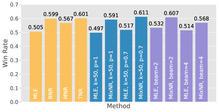
Figure 1: The effect of different generation configuration during inference and different negative sampling methods during training. Unless otherwise specified, greedy decoding is used. Win rate is evaluated by GPT-3.5 against the ground truth continuations.

Baselines.

We consider three main baselines: MLE, DPO, and parallel scheduled sampling (PSS, (Duckworth et al., 2019)). Importantly, the difference between DPO and CPO lies in their negative samples. For DPO, we query GPT-3.5 to generate unhelpful response to the Dolly instructions. PSS is trained to sample 3 sequences for each training data, and each token is replaced with $p=0.5$ (see Duckworth et al. (2019) for more details).

Table 1: The win rate of GPT2-XL against the ground truth, samples generated by greedy decoding, evaluated by GPT-3.5.

	MLE	PSS	DPO	ANR	MixNR
$\alpha$	-	-	-	-	0	0.5	0.7	0.9
WinRate	0.471	0.086	0.383	0.506	0.476	0.479	0.487	0.485

Training details.

Throughout the experiment, we fix the learning rate to be $1e-5$, we use the AdamW optimizer with weight decay of $0.05$. We keep the batch size to be $64$. Unless otherwise specified, for the baseline model, we train GPT2-XL and OpenLlama-3B with the next token prediction loss for $2000$ steps. Using these models as the reference model $\pi_{\operatorname{ref}}$, we continue to train with the CPO objective either with or without ranking signals, with $\beta=5$, for $1000$ steps. For both models, each training data in a batch contains $11$ negative samples in total. For MixN and MixNR, we also use a negative sample size of $11$, consisting of $3$ BN, $5$ MN, and $3$ TN. The MLE models used for evaluation are continually trained for the same number of steps from the reference model, like the CPO models. All experiments are conducted on two AWS machines, each with $8$ A100 GPUs.

Evaluation.

As discussed in Goyal et al. (2022), almost all automated evaluation metrics have been shown to not align with human evaluations in the modern era of LLMs, so we decide to use GPT (Brown et al., 2020) as the evaluator. See the query template in the appendix. For efficiency, we generate and evaluate $1000$ samples chosen from the 7506 test set. A similar template is used for Wiki text generation, see the detail in the appendix. During inference, we consider greedy decoding, top-$p$ and top-$k$ sampling, as well as beam search.

Table 2: The win rate of OpenLlama-3B trained with CPO and MLE against the ground truth data in Dolly, sampled by greedy decoding, evaluated by GPT-3.5. $\textsc{MLE}_{1}$, ANR and AN are trained for 200 steps, the rest models are trained for 1000 steps. The best CPO model outperforms the MLE baseline by 13.8% win rate.

	$\textsc{MLE}_{1}$	PSS	DPO	ANR	AN	$\textsc{MLE}_{2}$	MixNR						MixN
$\alpha$	-	-	-	-	-	-	0	0.1	0.3	0.5	0.7	0.9	-
WinRate	0.505	0.270	0.555	0.643	0.56	0.522	0.608	0.620	0.614	0.610	0.601	0.550	0.576

Weight-space ensemble.

Previous works (Liu et al., 2022) have also suggested to combine the auxilliary loss function with the MLE training objective $\alpha\mathcal{L}_{\mathrm{MLE}}+\mathcal{L}_{\mathrm{CPO}}$, the downside of combining loss functions in this way is that for a different choice of $\alpha$ one will have to retrain the model. To investigate the importance of loss combination, we instead perform a weight-space ensemble (Wortsman et al., 2022). In particular, denote $\theta_{\mathrm{CPO}}$ and $\theta_{\mathrm{MLE}}$ the model parameters trained solely with CPO or MLE respectively, we generate with the interpolated weights $\theta=\alpha\theta_{\mathrm{MLE}}+(1-\alpha)\theta_{\mathrm{CPO}}$.

5 Experimental Analysis

5.1 Instruction-Following Task

Our proposed CPO method with various negative sampling strategies consistently outperforms the MLE baseline models on the Dolly instruction-following task. Using greedy sampling with GPT2-XL, the CPO model has a clear margin over the MLE model, and CPO+ANR has a $3.5\%$ higher win rate, see table˜1. Note that CPO incurs very little computation overhead during the actual training: the overhead only comes a larger batch size, and even if we generate the negative samples autoregressively, it is a one-time offline cost.

The improvement in OpenLlama-3B is more significant: CPO+ANR has a $13.8\%$ higher win rate than the MLE baseline, and CPO+MixNR has a $9.8\%$ higher win rate in table˜2. We also observe that weight-space ensemble has a positive impact on the model. Heuristically, for OpenLlama-3B, a smaller $\alpha$ is preferred (more emphasis on the CPO weights) (table˜2), but the reverse holds for GPT2-XL (table˜1). We hypothesize that the choice of $\alpha$ should depend on the model: if the model is more capable, then it can benefit more from CPO. Here, we show the existence of a good $\alpha$, and we leave further exploration to future research.

Comparison with DPO and PSS.

The proposed CPO method performs better than other two baseline methods: DPO and PSS (see Table 2). We believe that DPO performs poorly because unhelpful/irrelevant continuations (even generated by ChatGPT) do not provide a very strong signal as human generated samples. Unlike in alignment, where the toxic/harmful samples provide a clear indication of what not to generate, here it is not clear what DPO can gain from merely a single irrelevant sample. On the other hand, CPO can benefit from larger negative sample size.

Sampling Strategy.

In addition to greedy decoding, we also experiment with different choice of sampling strategies. In all settings, CPO has consistently demonstrated superior performance over MLE, see fig.˜1.

Effect of different negative samples.

We perform a study on the effects of different negative sampling strategies; the results are presented in fig.˜1. We first train the OpenLlama-3B model with MLE loss for 1000 steps, then continue to train with CPO for 200 steps. For all ground truth sequences, we use $4$ negative sequences. In this setting, we always use the ranking information to train CPO. We observe that the effects of BNR and TNR on the reward model preference are similar and that they perform slightly better than MNR.

Table 3: OpenLlama-3B’s win rate against the ground truth continuation on Wikidump. The model is trained with either MLE or CPO+BNR. Weight ensemble is adopted. The best CPO model outperforms the MLE baseline by 3% win rate.

	MLE	BNR
$\alpha$	-	0	0.5	0.7	0.9
WinRate	0.508	0.455	0.505	0.5	0.538

5.2 Open-ended Text Generation Task

We further test OpenLlama-3B’s ability on an open-ended text generation task with CPO. Using Wikidump data (Foundation, ), for each test sample, we take its first $15\%$ tokens as the prefix and train the model with CPO on the rest $85\%$. For negative sampling, we use four BNR examples. The results in table˜3 show that CPO can improve the model’s win rate against the MLE baseline by $3\%$. We observe that increasing $\alpha$ improves the score, the opposite of the instruction-following task. It is likely because the negative samples here are too noisy, since only $15\%$ prefixes are provided.

Additionally, we test the MAUVE score (Pillutla et al., 2021) of MLE and CPO compared to the ground truth. See the results in fig.˜2 and table˜4.

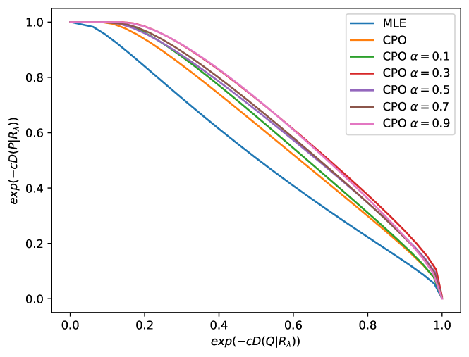
Figure 2: MAUVE score of MLE and CPO on Wiki data.

Table 4: MAUVE score of MLE and CPO on Wiki data.

	MLE	CPO BNR
$\alpha$	-	0	0.1	0.3	0.5	0.7	0.9
WinRate	0.524	0.610	0.627	0.673	0.645	0.651	0.668

6 Conclusions and Limitations

In this paper, we propose an auxiliary CPO loss function for LLM training, which can be used with or without ranking signals, depending on the quality of the negative samples. We investigated several ways to generate negative samples. One limitation of this work is that the synthetic data are very noisy unless generated autoregressively; it is interesting to explore other ways to efficiently generate high-quality negative data beyond the autoregressive fashion.

Appendix A Appendix

A.1 A brief introduction to DPO, RLHF, and EBM

The equivalence of RLHF and EBM

For the completeness of this paper, we include the result of the equivalence between RLHF and EBM. For the full proofs, we refer the reader to Rafailov et al. (2023); Korbak et al. (2022).

The RLHF objective is the following:

$$\begin{split}&\max_{\pi_{\theta}}\mathbb{E}_{{\bm{x}}\sim{\mathcal{D}},{\bm{y}}\sim\pi_{\theta}({\bm{y}}|{\bm{x}})}[r({\bm{x}},{\bm{y}})]\\ &\quad-\beta D_{\mathrm{KL}}\left(\pi_{\theta}({\bm{y}}|{\bm{x}})||\pi_{\operatorname{ref}}({\bm{y}}|{\bm{x}})\right),\end{split}$$ (3)

where ${\bm{x}}\sim\mathcal{D}$ is a given prefix, ${\bm{y}}\sim\pi_{\theta}({\bm{y}}|{\bm{x}})$ is a sampled continuation from the trainable model $\pi_{\theta}$, and $r({\bm{x}},{\bm{y}})\in\mathbb{R}$ is the reward. Meanwhile, we want to control the divergence between $\pi_{\theta}$ and $\pi_{\operatorname{ref}}$, where $\pi_{\operatorname{ref}}$ is usually an already pretrained or finetuned LLM. The RLHF optimum is achieved at the following EBM:

$$\pi^{*}({\bm{y}}|{\bm{x}})=\frac{1}{Z({\bm{x}})}\pi_{\operatorname{ref}}({\bm{y}}|{\bm{x}})\exp\left(\frac{1}{\beta}r({\bm{x}},{\bm{y}})\right),$$ (4)

where $Z({\bm{x}})=\sum_{{\bm{y}}}\pi_{\operatorname{ref}}({\bm{y}}|{\bm{x}})\exp\left(\frac{1}{\beta}r({\bm{x}},{\bm{y}})\right)$ is the partition function.

Rafailov et al. (2023) assume that the preference over two sequences ${\bm{y}}_{w}$ and ${\bm{y}}_{l}$ given ${\bm{x}}$ is parameterized by the Bradley-Terry model:

$$P({\bm{y}}_{w}\succ{\bm{y}}_{l}|{\bm{x}})=\frac{e^{r({\bm{x}},{\bm{y}}_{w})}}{e^{r({\bm{x}},{\bm{y}}_{l})}+e^{r({\bm{x}},{\bm{y}}_{w})}}.$$

Under the Bradley-Terry model, DPO establishes the equivalence between the original RLHF objective eq.˜3 and the following supervised objective:

$$\begin{split}&\mathcal{L}_{\mathrm{DPO}}(\pi_{\theta};\pi_{\text{ref}})=\\ &\mathbb{E}_{({\bm{x}},{\bm{y}}_{w},{\bm{y}}_{l})\sim\mathcal{D}}\Big{[}\log\sigma\Big{(}\beta\log\frac{\pi_{\theta}({\bm{y}}_{w}\mid{\bm{x}})}{\pi_{\text{ref}}({\bm{y}}_{w}\mid{\bm{x}})}\\ &\quad-\beta\log\frac{\pi_{\theta}({\bm{y}}_{l}\mid{\bm{x}})}{\pi_{\text{ref}}({\bm{y}}_{l}\mid{\bm{x}})}\Big{)}\Big{]},\end{split}$$ (5)

where $\sigma(\cdot)$ is the Sigmoid function.

They also generalize the formulation to the Plackett-Luce model, where we have a linear ordering $\tau(\cdot)$ among $K$ sequences:

Here, $\tau(1),\ldots,\tau(K)$ induce a ranking among $K$ sequences.

A.2 Derivation of the CPO objective function

Here we give a full derivation of the CPO objective function in eq.˜1.

Let ${\bm{y}}_{1},\ldots,{\bm{y}}_{K}$ be $K$ continuations of a given prefix ${\bm{x}}$. Without loss of generality, let ${\bm{y}}_{1}$ be the best candidate. We are interested in the MLE of the event $P({\bm{y}}_{1}\text{ is the best among $K$ candidates}|{\bm{x}})$.

We start from the sequence-level (RLHF) objective, notice that here $r(\cdot)$ is a reward over language quality, not human preference.

$$\begin{split}&\max_{\pi_{\theta}}\mathbb{E}_{{\bm{x}}\sim{\mathcal{D}},{\bm{y}}\sim\pi_{\theta}({\bm{y}}|{\bm{x}})}[r({\bm{x}},{\bm{y}})]\\ &\quad-\beta D_{\mathrm{KL}}\left(\pi_{\theta}({\bm{y}}|{\bm{x}})||\pi_{\operatorname{ref}}({\bm{y}}|{\bm{x}})\right),\end{split}$$ (7)

Its optimum is achieved at the following EBM:

$$\pi^{*}({\bm{y}}|{\bm{x}})=\frac{1}{Z({\bm{x}})}\pi_{\operatorname{ref}}({\bm{y}}|{\bm{x}})\exp\left(\frac{1}{\beta}r({\bm{x}},{\bm{y}})\right),$$ (8)

where $Z({\bm{x}})=\sum_{{\bm{y}}}\pi_{\operatorname{ref}}({\bm{y}}|{\bm{x}})\exp\left(\frac{1}{\beta}r({\bm{x}},{\bm{y}})\right)$ is the partition function. See the proof in Rafailov et al. (2023); Korbak et al. (2022).

Now we consider the natural extension of the Bradley-Terry model to $K$ candidates:

$$\begin{split}&P({\bm{y}}_{1}\text{ is the best among $K$ candidates}|{\bm{x}})\\ &=\frac{\exp\left(r^{*}({\bm{x}},{\bm{y}}_{1})\right)}{\sum_{k\in[K]}\exp\left(r^{*}({\bm{x}},{\bm{y}}_{k})\right)}.\end{split}$$ (9)

Now assuming we have the optimal policy $\pi^{*}$, we can reparameterize $r$ by rearranging eq.˜8:

$$\begin{split}r^{*}({\bm{x}},{\bm{y}})=\beta\log\frac{\pi^{*}({\bm{y}}\mid{\bm{x}})}{\pi_{\mathrm{ref}}({\bm{y}}\mid{\bm{x}})}+\beta\log Z({\bm{x}}).\end{split}$$ (10)

Plugging eq.˜10 into eq.˜9, we get eq.˜1.

A.3 Query template of Dolly and Wiki text generation

The query template for the Dolly instruction-following is the following: “For the following query to a chatbot, which response is more helpful?$\backslash$n Query: {}$\backslash$n Response A: {}$\backslash$n Response B: {}$\backslash$n State only "A" or "B" to indicate which response is more helpful.$\backslash$n More helpful:”

The template for Wiki is the following: “For the following prefix, which continuation is better?$\backslash$n Prefix: {}$\backslash$n Continuation A: {}$\backslash$n Continuation B: {}$\backslash$n State only "A" or "B" to indicate which continuation is more helpful.$\backslash$n Better:”

A.4 DPO generation template and example

When generating unhelpful responses for DPO, we query GPT with the following template: Given the ground truth instruction and response, can you generate a not helpful response?$\backslash$n Instruction: {}$\backslash$nResponse: {}$\backslash$nNot helpful response:.

One example of the generated response is the following: instruction: When did Virgin Australia start operating? chosen response: Virgin Australia commenced services on 31 August 2000 as Virgin Blue, with two aircraft on a single route. rejected response: Virgin Australia definitely exists and has airplanes that fly to different places.

A.5 Connection to noise contrastive estimation

Noise contrastrive estimation (NCE) (Gutmann and Hyvärinen, 2010) is a novel estimation technique introduced to tackle the computational infeasibility of traditional likelihood-based methods in large-scale machine learning models, particularly those involving high-dimensional data. NCE diverges from typical maximum likelihood estimation by transforming the problem into a classification task, which is deeply connected to both DPO and CPO. In NCE, the model is trained to distinguish between real data and noise/synthetic data. Beyond binary classification, RankingNCE also trains the model to rank the real data higher than all noise samples (Ma and Collins, 2018).

There are two important distinctions between CPO and NCE. First, instead of training the model to distinguish between real data and noise (at which any reasonable language model should already be good), we train the model to distinguish better than a reference model does, hence making the model better at recognizing natural text. Second, we also introduce a denser ranking signal by incorporating the similarity among embeddings of different samples. The experiments in this paper demonstrate that such a dense training signal consistently improves text generation quality.

References

- Arora et al. (2022) Kushal Arora, Layla El Asri, Hareesh Bahuleyan, and Jackie Chi Kit Cheung. 2022. Why exposure bias matters: An imitation learning perspective of error accumulation in language generation. arXiv preprint arXiv:2204.01171.
- Bengio et al. (2015) Samy Bengio, Oriol Vinyals, Navdeep Jaitly, and Noam Shazeer. 2015. Scheduled sampling for sequence prediction with recurrent neural networks. Advances in neural information processing systems, 28.
- Brown et al. (2020) Tom Brown, Benjamin Mann, Nick Ryder, Melanie Subbiah, Jared D Kaplan, Prafulla Dhariwal, Arvind Neelakantan, Pranav Shyam, Girish Sastry, Amanda Askell, et al. 2020. Language models are few-shot learners. Advances in neural information processing systems, 33:1877–1901.
- Chung et al. (2022) Hyung Won Chung, Le Hou, Shayne Longpre, Barret Zoph, Yi Tay, William Fedus, Eric Li, Xuezhi Wang, Mostafa Dehghani, Siddhartha Brahma, et al. 2022. Scaling instruction-finetuned language models. arXiv preprint arXiv:2210.11416.
- Conover et al. (2023) Mike Conover, Matt Hayes, Ankit Mathur, Jianwei Xie, Jun Wan, Sam Shah, Ali Ghodsi, Patrick Wendell, Matei Zaharia, and Reynold Xin. 2023. Free dolly: Introducing the world’s first truly open instruction-tuned llm.
- Deng et al. (2020) Yuntian Deng, Anton Bakhtin, Myle Ott, Arthur Szlam, and Marc’Aurelio Ranzato. 2020. Residual energy-based models for text generation. arXiv preprint arXiv:2004.11714.
- Duckworth et al. (2019) Daniel Duckworth, Arvind Neelakantan, Ben Goodrich, Lukasz Kaiser, and Samy Bengio. 2019. Parallel scheduled sampling. arXiv preprint arXiv:1906.04331.
- (8) Wikimedia Foundation. Wikimedia downloads.
- Geng and Liu (2023) Xinyang Geng and Hao Liu. 2023. Openllama: An open reproduction of llama.
- Goyal et al. (2022) Tanya Goyal, Junyi Jessy Li, and Greg Durrett. 2022. News summarization and evaluation in the era of gpt-3. arXiv preprint arXiv:2209.12356.
- Gutmann and Hyvärinen (2010) Michael Gutmann and Aapo Hyvärinen. 2010. Noise-contrastive estimation: A new estimation principle for unnormalized statistical models. In Proceedings of the thirteenth international conference on artificial intelligence and statistics, pages 297–304. JMLR Workshop and Conference Proceedings.
- Korbak et al. (2022) Tomasz Korbak, Ethan Perez, and Christopher L Buckley. 2022. Rl with kl penalties is better viewed as bayesian inference. arXiv preprint arXiv:2205.11275.
- Kumar et al. (2022) Sachin Kumar, Biswajit Paria, and Yulia Tsvetkov. 2022. Gradient-based constrained sampling from language models. In Proceedings of the 2022 Conference on Empirical Methods in Natural Language Processing, pages 2251–2277.
- Liu et al. (2022) Yixin Liu, Pengfei Liu, Dragomir Radev, and Graham Neubig. 2022. Brio: Bringing order to abstractive summarization. arXiv preprint arXiv:2203.16804.
- Ma and Collins (2018) Zhuang Ma and Michael Collins. 2018. Noise contrastive estimation and negative sampling for conditional models: Consistency and statistical efficiency. arXiv preprint arXiv:1809.01812.
- Ouyang et al. (2022) Long Ouyang, Jeffrey Wu, Xu Jiang, Diogo Almeida, Carroll Wainwright, Pamela Mishkin, Chong Zhang, Sandhini Agarwal, Katarina Slama, Alex Ray, et al. 2022. Training language models to follow instructions with human feedback. Advances in Neural Information Processing Systems, 35:27730–27744.
- Pace et al. (2024) Alizée Pace, Jonathan Mallinson, Eric Malmi, Sebastian Krause, and Aliaksei Severyn. 2024. West-of-n: Synthetic preference generation for improved reward modeling. arXiv preprint arXiv:2401.12086.
- Pang and He (2020) Richard Yuanzhe Pang and He He. 2020. Text generation by learning from demonstrations. arXiv preprint arXiv:2009.07839.
- Pillutla et al. (2021) Krishna Pillutla, Swabha Swayamdipta, Rowan Zellers, John Thickstun, Sean Welleck, Yejin Choi, and Zaid Harchaoui. 2021. Mauve: Measuring the gap between neural text and human text using divergence frontiers. Advances in Neural Information Processing Systems, 34:4816–4828.
- Radford et al. (2019) Alec Radford, Jeffrey Wu, Rewon Child, David Luan, Dario Amodei, Ilya Sutskever, et al. 2019. Language models are unsupervised multitask learners. OpenAI blog, 1(8):9.
- Rafailov et al. (2023) Rafael Rafailov, Archit Sharma, Eric Mitchell, Stefano Ermon, Christopher D Manning, and Chelsea Finn. 2023. Direct preference optimization: Your language model is secretly a reward model. arXiv preprint arXiv:2305.18290.
- Ranzato et al. (2015) Marc’Aurelio Ranzato, Sumit Chopra, Michael Auli, and Wojciech Zaremba. 2015. Sequence level training with recurrent neural networks. arXiv preprint arXiv:1511.06732.
- Sanh et al. (2021) Victor Sanh, Albert Webson, Colin Raffel, Stephen H Bach, Lintang Sutawika, Zaid Alyafeai, Antoine Chaffin, Arnaud Stiegler, Teven Le Scao, Arun Raja, et al. 2021. Multitask prompted training enables zero-shot task generalization. arXiv preprint arXiv:2110.08207.
- Schmidt (2019) Florian Schmidt. 2019. Generalization in generation: A closer look at exposure bias. arXiv preprint arXiv:1910.00292.
- Shen et al. (2015) Shiqi Shen, Yong Cheng, Zhongjun He, Wei He, Hua Wu, Maosong Sun, and Yang Liu. 2015. Minimum risk training for neural machine translation. arXiv preprint arXiv:1512.02433.
- Stiennon et al. (2020) Nisan Stiennon, Long Ouyang, Jeffrey Wu, Daniel Ziegler, Ryan Lowe, Chelsea Voss, Alec Radford, Dario Amodei, and Paul F Christiano. 2020. Learning to summarize with human feedback. Advances in Neural Information Processing Systems, 33:3008–3021.
- Touvron et al. (2023) Hugo Touvron, Thibaut Lavril, Gautier Izacard, Xavier Martinet, Marie-Anne Lachaux, Timothée Lacroix, Baptiste Rozière, Naman Goyal, Eric Hambro, Faisal Azhar, et al. 2023. Llama: Open and efficient foundation language models. arXiv preprint arXiv:2302.13971.
- Wang and Sennrich (2020) Chaojun Wang and Rico Sennrich. 2020. On exposure bias, hallucination and domain shift in neural machine translation. arXiv preprint arXiv:2005.03642.
- Wei et al. (2022) Jason Wei, Xuezhi Wang, Dale Schuurmans, Maarten Bosma, Fei Xia, Ed Chi, Quoc V Le, Denny Zhou, et al. 2022. Chain-of-thought prompting elicits reasoning in large language models. Advances in Neural Information Processing Systems, 35:24824–24837.
- Wettig et al. (2022) Alexander Wettig, Tianyu Gao, Zexuan Zhong, and Danqi Chen. 2022. Should you mask 15% in masked language modeling? arXiv preprint arXiv:2202.08005.
- Wortsman et al. (2022) Mitchell Wortsman, Gabriel Ilharco, Jong Wook Kim, Mike Li, Simon Kornblith, Rebecca Roelofs, Raphael Gontijo Lopes, Hannaneh Hajishirzi, Ali Farhadi, Hongseok Namkoong, et al. 2022. Robust fine-tuning of zero-shot models. In Proceedings of the IEEE/CVF Conference on Computer Vision and Pattern Recognition, pages 7959–7971.
- Zhang et al. (2019) Wen Zhang, Yang Feng, Fandong Meng, Di You, and Qun Liu. 2019. Bridging the gap between training and inference for neural machine translation. arXiv preprint arXiv:1906.02448.
- Zhou et al. (2023) Chunting Zhou, Pengfei Liu, Puxin Xu, Srini Iyer, Jiao Sun, Yuning Mao, Xuezhe Ma, Avia Efrat, Ping Yu, Lili Yu, et al. 2023. Lima: Less is more for alignment. arXiv preprint arXiv:2305.11206.