Network Tomography with Path-Centric Graph Neural Network

Abstract.

Network tomography is a crucial problem in network monitoring, where the observable path performance metric values are used to infer the unobserved ones, making it essential for tasks such as route selection, fault diagnosis, and traffic control. However, most existing methods either assume complete knowledge of network topology and metric formulas—an unrealistic expectation in many real-world scenarios with limited observability—or rely entirely on black-box end-to-end models. To tackle this, in this paper, we argue that a good network tomography requires synergizing the knowledge from both data and appropriate inductive bias from (partial) prior knowledge. To see this, we propose Deep Network Tomography (DeepNT), a novel framework that leverages a path-centric graph neural network to predict path performance metrics without relying on predefined hand-crafted metrics, assumptions, or the real network topology. The path-centric graph neural network learns the path embedding by inferring and aggregating the embeddings of the sequence of nodes that compose this path. Training path-centric graph neural networks requires learning the neural netowrk parameters and network topology under discrete constraints induced by the observed path performance metrics, which motivates us to design a learning objective that imposes connectivity and sparsity constraints on topology and path performance triangle inequality on path performance. Extensive experiments on real-world and synthetic datasets demonstrate the superiority of DeepNT in predicting performance metrics and inferring graph topology compared to state-of-the-art methods.

1. Introduction

Network tomography seeks to infer unobserved network characteristics using those that are observed. More specifically, one may observe path performance metrics (PPMs), such as path delay and capacity, by measuring the two endpoints of the path. Hence, network tomography can use the observations of the PPMs of some pairs of endpoints to infer those of the remaining pairs, because many PPMs can be written as aggregations of corresponding measures on the edges which are typically far fewer the paths they can make up. Network tomography plays a crucial role in applications such as route selection (Ikeuchi et al., 2022; Tao et al., 2024), fault diagnosis (Ramanan et al., 2015; Qiao et al., 2020), and traffic control (Zhang et al., 2018; Pan et al., 2020; Lev-Ari et al., 2023). In real-world applications, many network characteristics are inaccessible. For example, in a local area network connected to the Internet, internal devices remain hidden due to security policies (Figure 1), necessitating network tomography to infer path-related states like latency and congestion (Cao and Sun, 2012). Similar challenges arise in transportation networks for estimating arrival times and traffic conditions (Zhang et al., 2018), and in social networks for uncovering hidden connections (Xing et al., 2009).

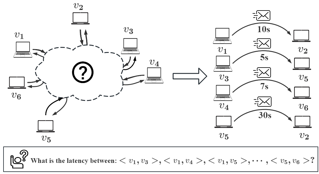
Figure 1. An illustration of network tomography in a sample network, where the end-to-end latency needs to be predicted when the network topology is not available.

Network tomography is very challenging since the PPM values of a pair of nodes are jointly determined by the specific path in a particular network topology under a certain PPM type. To make this problem solvable, traditional network tomography approaches rely on the observed network topology and predefined, hand-crafted PPM calculations, focusing on either additive metrics, where the combined metric over a path is the sum of the involved link metrics (e.g., delay), or non-additive metrics, where the path performance is a nonlinear combination of link metrics (Feng et al., 2020; Xue et al., 2022). Other prescribed methods depend on assumptions like rare simultaneous failures (Lai and Baker, 2000; Carter and Crovella, 1996; Jain and Dovrolis, 2002), minimal sets of network failures (Duffield, 2003, 2006; Kompella et al., 2007), or sparse performance metrics (Zhang et al., 2009; Firooz and Roy, 2010; Xu et al., 2011). These methods rely heavily on human-defined heuristics and rules, making their inference limited and biased by human domain knowledge, especially for many areas where we do not know what PPMs best model the network process. For instance, a heuristic rule that assumes rare simultaneous network failures may be effective for localizing network bottlenecks in a computer network, but would not be suitable for environments like cloud computing or distributed systems, where performance degradation often involves multiple simultaneous disruptions across different nodes or links. More recently, dynamic routing (Tagyo et al., 2021; Sartzetakis and Varvarigos, 2023) and deep learning approaches (Ma et al., 2020; Sartzetakis and Varvarigos, 2022; Tao and Silvestri, 2023) have attempted to bypass the need for prior knowledge on PPMs by directly learning end-to-end models from data (e.g., predicting PPMs given the path’s two endpoints). Hence, although they avoided traditional methods’ heavy dependency on the observed network topology and prior knowledge of PPMs, they went to the other extreme, by typically completely overlooking the prior knowledge of the PPMs and the intrinsic relation between paths and edges.

To overcome the complementary drawbacks of traditional and deep learning-based methods, we pursue our method, Deep Network Tomography (DeepNT), which can infer the network topology and how it determines the PPMs, by deeply characterizing the network process by eliciting and synergizing the knowledge from both training data and partial knowledge of the inductive bias of PPMs. More concretely, we propose a new path-centric graph neural network that can infer the PPMs values of a path by learning its path embedding composed by the inferred sequence of node embeddings along this path. Training path-centric graph neural networks requires learning the neural network parameters and network topology following mixed connectivity constraint and path performance traignle inequailty constraints.

In summary, our primary contributions are as follows:

• New Problem. We formulate the learning-based network tomography problem as learning representations for end-node pairs to simplify the optimization and identify unique challenges that arise in its real-world applications.

• New Computational Framework. We propose a novel model for inferring unavailable adjacency matrices and metrics of unmeasured paths, learning end-node pair representations in an end-to-end manner.

• New Optimization Algorithm. We propose to infer adjacency matrices with strongly and weakly connectivity constraints and a triangle inequality constraint. We proposed to transfer the discrete connectivity constraints into continuous forms for numerical optimization.

• Extensive Experiment Evaluation. Extensive experiments on real-world and synthetic datasets demonstrate the outstanding performance of DeepNT. DeepNT outperforms other state-of-the-art models in predicting different path performance metrics as well as reconstructing network adjacency matrices.

2. Related Work

2.1. Network Tomography

Network Tomography involves inferring internal network characteristics using performance metrics, which can be broadly classified as additive or non-additive. Additive metrics frame the network tomography problem as a linear inverse problem, often assuming a known network topology and link-path relationships (Gurewitz and Sidi, 2001; Liang and Yu, 2003; Chen et al., 2010). Statistical methods such as Maximum Likelihood Estimation (MLE) (Wandong et al., 2011; Teng et al., 2024), Expectation Maximization (EM) (Bu et al., 2002; Wei et al., 2007; Wandong et al., 2011), and Bayesian estimation (Zhang, 2006; Wandong et al., 2011) are employed to solve this problem. Algebraic approaches, such as System of Linear Equations (SLE) (Bejerano and Rastogi, 2003; Chen et al., 2003; Gopalan and Ramasubramanian, 2011) and Singular Value Decomposition (SVD) (Chua et al., 2005; Song et al., 2008), that rely on traceroute work well in certain scenarios but are often blocked by network providers to maintain the confidentiality of their routing strategies. When link performance metrics are sparse, compressive sensing techniques are used to identify all sparse link metrics (Firooz and Roy, 2010; Xu et al., 2011). Furthermore, studies have explored the sufficient and necessary conditions to identify all link performance metrics with minimal measurements (Gopalan and Ramasubramanian, 2011; Alon et al., 2014). Non-additive metrics, such as boolean metrics, introduce additional complexity and constraints. These studies often assume that multiple simultaneous failures are rare, focusing on identifying network bottlenecks (Bejerano and Rastogi, 2003; Horton and López-Ortiz, 2003). However, the assumption of rare simultaneous failures is not always valid. Some works address this by identifying the minimum set of network failures or reducing the number of measurements required (Duffield, 2006; Zeng et al., 2012; Ikeuchi et al., 2022). Additionally, several papers have proposed conditions and algorithms to efficiently detect network failures (He, 2018; Galesi and Ranjbar, 2018; Bartolini et al., 2020; Ibraheem et al., 2023), and some studies have attempted to apply deep learning to this field (Ma et al., 2020; Sartzetakis and Varvarigos, 2022; Tao and Silvestri, 2023). However, most existing works rely on hand-crafted rules and specific assumptions, making them specialized for certain applications and unsuitable where prior knowledge of network properties or topology is unavailable.

2.2. GNNs for Graph Structure Learning

GNNs for Graph Structure Learning can be classified into approaches for learning discrete graph structures (i.e., binary adjacency matrices) and weighted graph structures (i.e., weighted adjacency matrices). Discrete graph structure approaches typically sample discrete structures from learned probabilistic adjacency matrices and subsequently feed these graphs into GNN models. Notable methods in this category include variational inference (Chen et al., 2018), bilevel optimization (Franceschi et al., 2019), and reinforcement learning (Kazemi et al., 2020). However, the non-differentiability of discrete graph structures poses significant challenges, leading to the adoption of weighted graph structures, which encode richer edge information. A common approach involves establishing graph similarity metrics based on the assumption that node embeddings during training will resemble those during inference. Popular similarity metrics include cosine similarity (Nguyen and Bai, 2010), radial basis function (RBF) kernel (Yeung and Chang, 2007), and attention mechanisms (Chorowski et al., 2015). While graph similarity techniques are applied in fully-connected graphs, graph sparsification techniques explicitly enforce sparsity to better reflect the characteristics of real-world graphs (Chen et al., 2020b; Jin et al., 2020). Additionally, graph regularization is employed in GNN models to enhance generalization and robustness (Chen et al., 2020a). In this work, we leverage GNNs to learn end-node pair representations, enabling simultaneous prediction of path performance metrics and inference of the network topology.

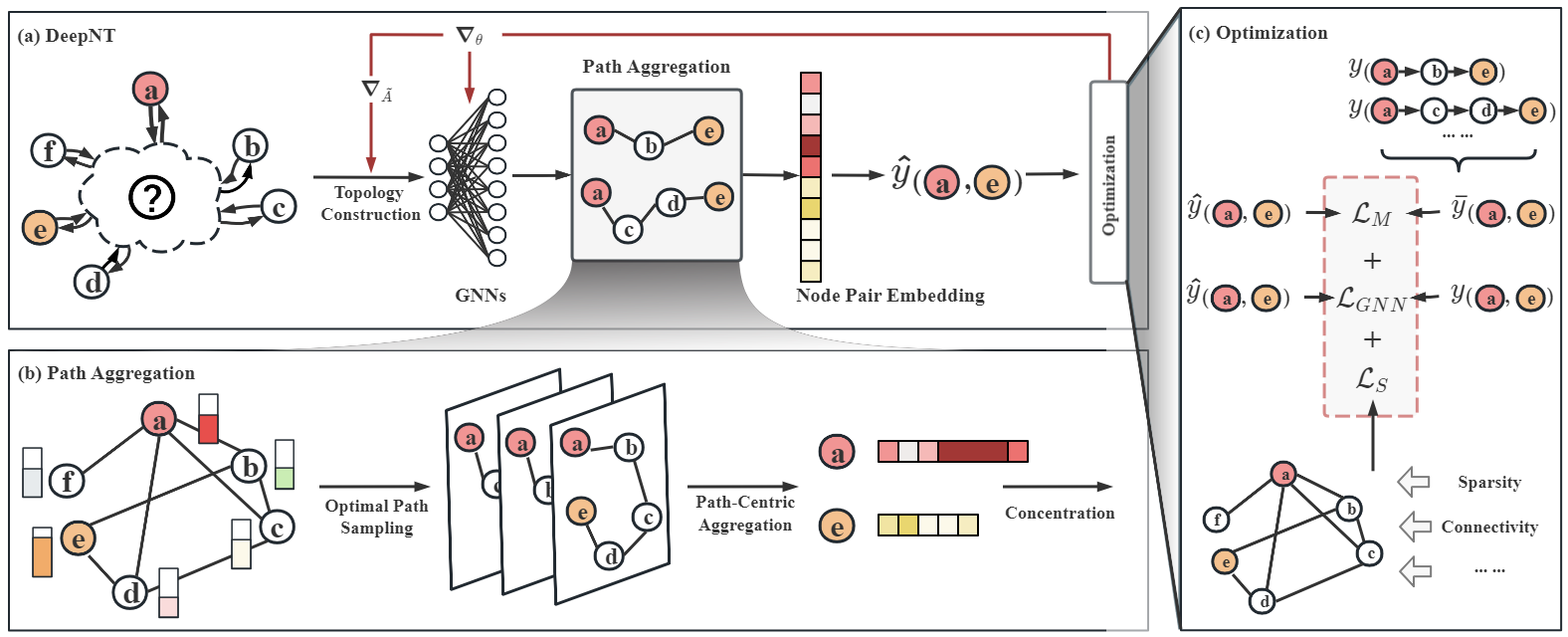
Figure 2. Overall framework of proposed deep network tomography solution.

3. Problem Formulation

Graphs. A connected network $\mathcal{G}$ is defined as $\mathcal{G}=(V,E)$, where $V$ and $E\subseteq V\times V$ represent the node set and edge set, respectively, let $A$ denote the adjacency matrix of $\mathcal{G}$.

Path Performance Metrics (PPMs). Given a graph $\mathcal{G}=(V,E)$, let $\mathcal{P}_{uv}=\{p_{uv}^{n}\}_{n=1}^{N}$ represent the set of all possible paths from node $u$ to $v$, where $u,v\in V$, and $N$ denotes the number of possible paths between $u$ and $v$. Let $y_{e}$ be the performance metric value of an individual edge, where $e\in E$. The path performance metric value is defined as the cumulative performance of all edges on a path, where the cumulative calculation depends on the type of metric being considered. The unified path performance metric is defined as follows:

(1) $$y_{uv}^{n}=\mathop{\bigotimes}\limits_{e_{i}\in p_{uv}^{n}}y_{e_{i}},~\text{where}~\bigotimes\in\{\sum,\prod,\bigwedge,\bigvee,\min,\cdots\},$$

where $\bigotimes$ represents an operator that varies based on the type of path performance metrics, such as additive, multiplicative, boolean, min/max, etc. The optimal path performance between two nodes is defined as $y_{uv}=\{y_{uv}^{n}\mid y_{uv}^{n}\mathbin{\scalerel*{\ensurestackMath{\stackon[0pt]{\geqq}{\ThisStyle{\raisebox{-0.7pt}{\scalebox{1.45}{$\SavedStyle\bigcirc$}}}}}}{\ThisStyle{\raisebox{-0.7pt}{\scalebox{1.45}{$\SavedStyle\bigcirc$}}}}}y_{uv}^{k},~\forall p_{uv}^{k}\neq p_{uv}^{n}\in\mathcal{P}_{uv}\}$, where $\mathbin{\scalerel*{\ensurestackMath{\stackon[0pt]{\geqq}{\ThisStyle{\raisebox{-0.7pt}{\scalebox{1.45}{$\SavedStyle\bigcirc$}}}}}}{\ThisStyle{\raisebox{-0.7pt}{\scalebox{1.45}{$\SavedStyle\bigcirc$}}}}}$ indicates better performance, depending on the specific type of path performance metric. For additive metrics like latency, $\bigotimes=\sum$ and $\mathbin{\scalerel*{\ensurestackMath{\stackon[0pt]{\geqq}{\ThisStyle{\raisebox{-0.7pt}{\scalebox{1.45}{$\SavedStyle\bigcirc$}}}}}}{\ThisStyle{\raisebox{-0.7pt}{\scalebox{1.45}{$\SavedStyle\bigcirc$}}}}}=\leq$, where the path metric is the sum of edge latencies, with lower values indicating better performance. For min metrics like capacity, $\bigotimes=\min$ and $\mathbin{\scalerel*{\ensurestackMath{\stackon[0pt]{\geqq}{\ThisStyle{\raisebox{-0.7pt}{\scalebox{1.45}{$\SavedStyle\bigcirc$}}}}}}{\ThisStyle{\raisebox{-0.7pt}{\scalebox{1.45}{$\SavedStyle\bigcirc$}}}}}=\max$, where the minimum capacity along the path defines overall path performance, and higher values are preferable.

Network Tomography. Define $T=\{\langle u,v\rangle\}_{u\neq v\in V}$ as the set of all node pairs, where $|T|=\binom{|V|}{2}$. Let $S\subset T$ be a subset of node pairs for which the end-to-end optimal PPMs are measured. The exact path information between any two nodes is unknown. Network tomography aims to use the measured PPMs values in $S$ to predict the end-to-end optimal PPMs value of unmeasured node pairs in $T\setminus S$. The optimal path between two nodes is typically determined by the Best Performance Routing (BPR). For instance, in a computer network, with measured end-to-end transmission delays for certain node pairs $S\subset T$, the goal of network tomography is to infer the minimum delays for the unmeasured pairs in $T\setminus S$, when the exact path information for node pairs in $T\setminus S$ is unknown.

4. Deep Network Tomography

Overview. Network tomography is very challenging since the PPM values of a pair of nodes are jointly determined by the specific path in a particular network topology under a certain PPM type. Hence, we propose a DeepNT to jointly infer network topology, consider path candidates, and learn path performance metrics, in order to effectively predict the PPM values of a node pair. Specifically, we propose a path-centric graph neural network to learn the candidate paths’ embedding from the embeddings of the nodes on them and then aggregate them into node pair embedding for the final PPM value prediction, as illustrated in Figure 2(a) and detailed in Section 4.1. To infer the network topology, DeepNT introduces a learning objective (Figure 2(c)) that updates the adjacency matrix of the network by imposing constraints on connectivity and sparsity, as detailed in Section 4.3. This allows for the simultaneous prediction of PPM values and inference of network structure. Moreover, to leverage the inductive bias inherent in different types of PPMs, we introduce path performance triangle inequalities that further refine our predictions, as outlined in Section 4.2.

4.1. Path-Centric Graph Neural Network

Candidate paths’ information elicitation and encoding. Due to unknown paths from partial network topology, we aggregate multiple potential paths to capture PPM context. Specifically, for each node pair, e.g., $\langle u,v\rangle$, we leverage BPR to sample $N$ loopless paths between them based on the adjacent matrix $\tilde{A}$, denoted as $\mathcal{P}_{uv}^{L}=\{p_{uv}^{(n)}\}_{n\in[1,N]}$, ensuring that the lengths do not exceed $L$. Then, the node embeddings of $u$ and $v$ are updated with a path aggregation layer. For node $v$, we first compute the attention scores between $v$ and all nodes along the path from $v$ to $u$:

(2) $$e^{(n)}_{vz}=\sigma(r^{\top}[(h_{v},h^{(n)}_{z}])\Longrightarrow~\alpha^{(n)}_{vz}=\text{softmax}(e^{(n)}_{vz}),$$

where $z\in p^{(n)}_{uv}$, $\sigma$ is an activation function, and $r$ is a predefined vector. We then aggregate path information to obtain path-centric node pair embeddings:

(3) $$\hat{h}^{(n)}_{v}=h_{v}+\sigma\bigg{(}\sum\nolimits_{z\in p^{(n)}_{uv}}\alpha^{(n)}_{vz}h^{(n)}_{z}\bigg{)},$$

(4) $$\hat{h}_{v}=\text{READOUT}(\{\hat{h}^{(n)}_{v}\mid p^{(n)}_{uv}\in\mathcal{P}_{uv}^{L}\}),$$

where $\text{READOUT}(\cdot)$ is a permutation-invariant function. $\hat{h}_{u}$ is obtained in the same way. This path-centric embedding aggregates the local neighborhood information of the end-node pair as well as the information in potential optimal paths connecting them. Finally, the concatenated representation of the end-node pair is passed through a projection module to predict the performance metric value $\hat{y}_{uv}$ via $f_{\theta}:(u,v,\tilde{A})\rightarrow\hat{y}_{uv}$. The objective function can be formulated as,

(5) $$\min_{\theta,\tilde{A}}\mathcal{L}_{GNN}(\theta,\tilde{A},Y)=\sum_{u,v\in V}l(f_{\theta}(u,v,\tilde{A}),y_{uv}),~s.t.,~\tilde{A}\in\mathcal{A},\vskip-3.0pt$$

where $\theta$ indicates the parameters of $f(\theta)$, $l(\cdot,\cdot)$ is to measure the difference between the prediction $f_{\theta}(u,v,\tilde{A})$ and the target value $y_{uv}$, e.g., cross entropy for boolean metrics and $\ell_{2}$ norm for additive metrics. Another objective will be introduced in following Section 4.3 to infer a optimal symmetric adjacency matrix $\tilde{A}\in\mathcal{A}$ where $\mathcal{A}$ represents the set of valid adjacency matrices specified in Section 4.3. We then introduce a training penalty that constrains the DeepNT model with a path performance triangle inequality, applicable to any type of path performance metric.

Let $\mathcal{AP}$ denote the set of all possible paths between node pair combinations. DeepNT-$\mathcal{AP}$, utilizing the proposed path-centric aggregation with access to $\mathcal{AP}$, effectively distinguishes node pairs.

Theorem 4.1 (DeepNT-$\mathcal{AP}$ Distinguishes Node Pairs Beyond 1-WL).

Let $G=(V,E)$, and let $\langle u,v\rangle$ and $\langle u^{\prime},v^{\prime}\rangle$ be two node pairs in $V\times V$ such that the local neighborhoods of $u$ and $u^{\prime}$ are identical up to $L$ hops, and similarly for $v$ and $v^{\prime}$. If the sets of paths $\mathcal{P}_{uv}^{L}$ and $\mathcal{P}_{u^{\prime}v^{\prime}}^{L}$ are different, DeepNT will assign distinct embeddings $f_{\text{DeepNT}}(u,v)\neq f_{\text{DeepNT}}(u^{\prime},v^{\prime})$.

The analysis of DeepNT’s expressive power and the proof of Theorem 4.1 are provided in Appendix A.4.

4.2. Path Performance Triangle Inequality

Since PPM is for the optimal path among all the paths between the node pairs, the performance of any path between these two nodes cannot exceed the performance of the observed optimal path. For each pair of nodes $u$ and $v$, and for any other node $z$ on the path, the following triangle inequality must hold: $y_{uv}\mathbin{\scalerel*{\ensurestackMath{\stackon[0pt]{\geqq}{\ThisStyle{\raisebox{-0.7pt}{\scalebox{1.45}{$\SavedStyle\bigcirc$}}}}}}{\ThisStyle{\raisebox{-0.7pt}{\scalebox{1.45}{$\SavedStyle\bigcirc$}}}}}(y_{uz}\bigotimes y_{zv}$) because $y_{uv}$, corresponding to the best path between $\langle u,v\rangle$, should be no worse than $y_{uz}\bigotimes y_{zv}$, the best path between $\langle u,v\rangle$ going through $z$. Here, $\mathbin{\scalerel*{\ensurestackMath{\stackon[0pt]{\geqq}{\ThisStyle{\raisebox{-0.7pt}{\scalebox{1.45}{$\SavedStyle\bigcirc$}}}}}}{\ThisStyle{\raisebox{-0.7pt}{\scalebox{1.45}{$\SavedStyle\bigcirc$}}}}}$ is a generalized inequality relation that will be specified according to the type of PPM of interest. For example, when the performance metric is delay (where better performance corresponds to lower values), $\mathbin{\scalerel*{\ensurestackMath{\stackon[0pt]{\geqq}{\ThisStyle{\raisebox{-0.7pt}{\scalebox{1.45}{$\SavedStyle\bigcirc$}}}}}}{\ThisStyle{\raisebox{-0.7pt}{\scalebox{1.45}{$\SavedStyle\bigcirc$}}}}}$ becomes $\leq$. Thus, we will only punish the violation of the above generalized inequality, resulting in the following generalized ReLU style loss given $f_{\theta}(u,v)=\hat{y}_{u,v}$:

(6) $$\min_{\theta,\tilde{A}}\mathcal{L}_{M}(\theta,\tilde{A},Y)=\sum_{u,v\in V}l_{M}(f_{\theta}(u,v,\tilde{A}),y_{uz}\bigotimes y_{zv}),\vskip-3.0pt$$

where $z$ is a random node in $p^{(n)}_{uv}$, and $p^{(n)}_{uv}$ is the path with the optimal performance in $\mathcal{P}_{uv}^{L}$. The function $l_{M}$ computes a penalty enforcing that the predicted performance does not exceed the bounded value, defined as $l_{M}(\hat{y},y)=\max(0,\hat{y}\ominus y)$, where $\ominus$ is also chosen adaptively based on the type of path performance metric. As a result, the estimated performance metric is always bounded by the optimal performance among the observed paths.

4.3. Graph Structure Completion

Real-world networks are typically sparse, noisy, connected, and partially unobservable (Zhou et al., 2013; Fan and Li, 2017), making accurate topology learning essential for network tomography. The learned adjacency matrix must ensure reachability of observed node pairs while preserving sparsity and connectivity. Given an observed network adjacency matrix $A$, we formulate this process as a structure learning problem:

(7) $$\min_{\tilde{A}}\mathcal{L}_{S}=\|\mathcal{R}(M\odot\tilde{A})-\mathcal{R}(A)\|_{F}^{2}+S(\tilde{A}),\quad\text{s.t.}~\tilde{A}\in\mathcal{A},$$

where $\mathcal{R}(A)$ maps $A$ to a binary matrix indicating the existence of paths between node pairs. $M\in\{0,1\}^{|V|\times|V|}$ marks observed edge connectivity, and $\|\cdot\|_{F}^{2}$ ensures the learned adjacency matrix $\tilde{A}$ preserves the observed pairwise reachability. $S(\tilde{A})$ imposes constraints to enforce both connectivity and sparsity. To encourage sparsity, we minimize the $\ell_{1}$-norm, which promotes a sparse adjacency structure (Candes and Recht, 2012; Tsybakov et al., 2011).

For connectivity, although the network topology is unknown or partially incorrect, the existence of at least one path between observed node pairs ensures the graph is weakly connected. PPMs further guarantee path reachability, allowing us to infer structural properties and detect Strongly Connected Components (SCCs) by Tarjan’s Algorithm (Tarjan, 1972). The challenge lies in embedding this prior knowledge into Equation (7), as enforcing connectivity constraints is inherently discrete. To enable gradient-based optimization, we transform these constraints into a continuous form through a novel convex formulation that encodes both weak connectivity and SCCs, as detailed in Theorem 4.2.

Theorem 4.2 (Directed Graph Connectivity Constraints).

Let $G=(V,E)$ be a directed graph with a non-negative adjacency matrix $A_{G}\in\mathbb{R}^{|V|\times|V|}$. For any graph with adjacency matrix $A\in\mathbb{R}^{n\times n}$, define:

$$Z_{A}=\operatorname{diag}\left(A\cdot\mathbf{1}^{\top}\right)-A+\frac{1}{|n|}\mathbf{1}\mathbf{1}^{\top},$$

where $\mathbf{1}\in\mathbb{R}^{|n|}$ is an all-ones vector. Let $\mathcal{G}$ denote the set of SCCs identified via PPMs. The entire graph is weakly connected, with each SCC $g\in\mathcal{G}$ strongly connected, if and only if:

1. $Z_{A_{G}}\succ 0,\quad A\geq 0,$

2. $Z_{A_{g}}+Z_{A_{g}}^{\top}\succ 0,\quad A_{g}\geq 0,\forall g\in\mathcal{G},$

where $A_{g}$ is the adjacency matrix of component $g$.

The proof can be found in Appendix A.5. Incorporating the connectivity constraints from Theorem 4.2 and the sparsity constraints on the inferred adjacency matrices $\tilde{A}$ and $\tilde{A}_{g}$ for the graph and components $g\in\mathcal{G}$, the topological constraint $S(\tilde{A})$ for DeepNT is derived, and Equation 7 is reformulated as:

(11) $$\begin{gathered}\min_{\tilde{A}}\|\mathcal{R}(M\odot\tilde{A})-\mathcal{R}(A)\|_{F}^{2}+\alpha\|\tilde{A}\|_{1},\\[-5.0pt] \text{s.t.}\quad\operatorname{diag}(\tilde{A}\cdot\mathbf{1}^{\top})-\tilde{A}+\mathbf{1}^{\top}\mathbf{1}/|V|\succ 0,~\tilde{A}\geq 0,\tilde{A}\in\mathcal{A}\\ \operatorname{diag}(\tilde{A}_{g}\cdot\mathbf{1}^{\top})-\operatorname{Sym}(\tilde{A}_{g})+\mathbf{1}^{\top}\mathbf{1}/|g|\succ 0,~\forall g\in\mathcal{G},\tilde{A}_{g}\geq 0.\end{gathered}$$

where $\operatorname{Sym}(A)=(A+A^{\top})/2$ means the symmetrization of matrix $A$, $\alpha$ controls the contribution from the sparsity constraint.

4.4. Optimization for DeepNT

Based on the defined constraints, we formulate the optimization of DeepNT as a continuous optimization problem solvable via gradient descent. We jointly learn the GNN model and the adjacency matrix to infer the optimal network topology for the GNN model. The final objective function of DeepNT is given as,

(12) $$\operatorname*{min}_{\theta,\tilde{A}}\mathcal{L}=\mathcal{L}_{GNN}+\mathcal{L}_{S}+\gamma\mathcal{L}_{M}$$

$$\text{s.t.}\quad\operatorname{diag}((\tilde{A}+ \tilde{A}^{\top})/2\cdot\mathbf{1}^{\top})-(\tilde{A}+\tilde{A}^{\top})/2+\mathbf{1}^{\top}\mathbf{1}/|V|\succ 0,~\tilde{A}\in\mathcal{A},$$

where $\gamma$ is a predefined parameter. Jointly optimizing $\theta$ and $\tilde{A}$ is challenging because it involves navigating a highly non-convex optimization landscape with interdependent variables. The optimization problem in DeepNT is formulated as follows:

(13) $$\mathcal{F}=\min_{\theta,\tilde{A}}g(\theta,\tilde{A})+\alpha||\tilde{A}||_{1},$$

where $g(\theta,\tilde{A})=\mathcal{L}_{GNN}+\gamma\mathcal{L}_{M}+\|\mathcal{R}(M\odot\tilde{A})-\mathcal{R}(A)\|_{F}^{2}$. To facilitate effective learning, we introduce a proximal gradient algorithm with extrapolation, as detailed in Algorithm 1, where the graph is constrained to be weakly connected, $\operatorname{prox}_{\lambda\|\cdot\|_{1}}(f)=S_{\lambda}(f)=\arg\min\nolimits_{x}\left(\frac{1}{2}\|x-f\|_{F}^{2}+\lambda\|x\|_{1}\right)$ is the soft-thresholding operator. The algorithm initializes $\theta$ and $\tilde{A}$ (line 1), then iteratively updates parameters via gradient descent and optimizes $\tilde{A}$ with proximal and connectivity constraints (lines 2-19) until convergence.

Convergence of our optimization algorithm is guaranteed by Theorem 4.3, whose proof is provided in Appendix A.6.

Theorem 4.3.

Assume $g(\theta,\tilde{A})$ is Lipschitz continuous with coefficient $l>0$, and its gradient $\nabla g(\theta,\tilde{A})$ is Lipschitz continuous with coefficient $L>0$. Let $\frac{1}{L}\leq\omega\leq\sqrt{\frac{L}{L+l}}$, and let $\{(\theta^{k},\tilde{A}^{k})\}$ be a sequence generated by Algorithm 1, then any of its limit point $(\theta^{*},\tilde{A}^{*})$ is a stationary point of Equation (13).

We demonstrate that DeepNT’s network tomography capabilities are guaranteed under sufficient observations, as established in Theorem 4.4.

Theorem 4.4 (Convergence of DeepNT Predictions to True Pairwise Metrics).

Let $G=(V,E)$. Suppose DeepNT is trained with an increasing number of observed node pairs $S\to T$, where $S\subseteq T=V\times V$, and the number of sampled paths $N\to\infty$. Then, the predicted pairwise metrics $\hat{y}_{uv}=f_{\text{DeepNT}}(u,v;\theta,\tilde{A})$ converge in expectation to the true metrics $y_{uv}$, i.e.,

$$\lim_{S\to T}\lim_{N\to\infty}\mathbb{E}_{\langle u,v\rangle\sim T}\left[\lvert\hat{y}_{uv}-y_{uv}\rvert\right]=0,$$

The proof of Theorem 4.4 is detailed in Appendix A.7.

Algorithm 1 Optimization of DeepNT

1:Input data $S$, labels $y$, momentum parameter $\omega$, graph components $\mathcal{G}$

2:Parameters $\theta$ of DeepNT, inferred adjacency matrix $\tilde{A}$

3:$\tilde{A}^{-1}\leftarrow 0$, $\tilde{A}^{0}\leftarrow 0$, $\theta^{-1}\leftarrow 0$, $\theta^{0}\leftarrow 0$

4:while stopping condition is not met do

5:  $\triangleright$ Momentum-accelerated updates for parameters and adjacency matrix.

6:  $\overline{\theta}^{k}\leftarrow\theta^{k}+(1-\omega)(\theta^{k}-\theta^{k-1})$

7:  $\overline{A}^{k}\leftarrow\tilde{A}^{k}+(1-\omega)(\tilde{A}^{k}-\tilde{A}^{k-1})$

8:  $\triangleright$ Gradient descent update for model parameters.

9:  $\theta^{k+1}\leftarrow\overline{\theta}^{k}-\omega\nabla g(\overline{\theta}^{k},\overline{A}^{k})$

10:  $\triangleright$ Proximal optimization for the global adjacency matrix.

11:  $\tilde{A}^{k+1}\leftarrow\operatorname{prox}_{\omega\alpha\|\cdot\|_{1}}\left(\overline{A}^{k}-\omega\nabla g(\overline{\theta}^{k},\overline{A}^{k})\right)$

12:  $\triangleright$ Enforce global connectivity constraint on $\tilde{A}^{k+1}$.

13:  $\Delta\tilde{A}\leftarrow\operatorname{diag}(\operatorname{Sym}(\tilde{A}^{k+1})\cdot\mathbf{1}^{\top})-\operatorname{Sym}(\tilde{A}^{k+1})+\mathbf{1}^{\top}\mathbf{1}/|V|$

14:  $\tilde{A}^{k+1}\leftarrow\operatorname{prox}_{\succ}(\Delta\tilde{A})$

15:  $\triangleright$ Proximal updates and connectivity enforcement.

16:  for each $g\in\mathcal{G}$ do

17:   $\tilde{A}_{g}^{k+1}\leftarrow\operatorname{prox}_{\omega\alpha\|\cdot\|_{1}}\left(\tilde{A}_{g}^{k}-\omega\nabla g(\overline{\theta}^{k},\tilde{A}_{g}^{k})\right)$

18:   $\Delta\tilde{A}_{g}\leftarrow\operatorname{diag}(\operatorname{Sym}(\tilde{A}_{g}^{k+1})\cdot\mathbf{1}^{\top})-\operatorname{Sym}(\tilde{A}_{g}^{k+1})+\mathbf{1}^{\top}\mathbf{1}/|g|$

19:   $\tilde{A}_{g}^{k+1}\leftarrow\operatorname{prox}_{\succ}(\Delta\tilde{A}_{g})$

20:  end for

21:end while

5. Experiment

5.1. Datasets

We conduct experiments on three real-world datasets, encompassing transportation, social, and computer networks, each characterized by distinct path performance metrics. Transportation networks are collected from different cities. The social network dataset collects interactions between people on different online social platforms, including Epinions, Facebook and Twitter. The Internet dataset consists of networks with raw IPv6 or IPv4 probe data. Details on data statistics, data processing, and path performance metrics for each dataset can be found in Appendix A.1.

We use a synthetic dataset to test the comprehensive performance of our model on networks of different sizes and properties, exploring the robustness and scalability of our model. Synthetic networks are generated using the Erdős-Rényi, Watts-Strogatz and Barabási–Albert models. For network sizes in ${50i}_{i=1}^{50}$, each graph generation algorithm is used to generate 10 networks with varying edge probabilities for each network size (the edge probability represents the likelihood that any given pair of nodes in the network is directly connected by an edge). We focus on monitor-based sampling scenarios, where some nodes are randomly selected as monitors and the end-to-end path performance between the monitors and other nodes are sampled as training data. For all datasets, we set different sampling rates $\delta\in\{10\%,20\%,30\%\}$ to simulate the real network detection scenario (Ma et al., 2020). The sampled path performance is used as training data, that is, $\delta$ of total node pairs are used as training data and the rest of node pairs are used for testing.

Table 1. Mean Absolute Percentage Error (MAPE $\downarrow$) and Mean Squared Error (MSE $\downarrow$) for Additive Metrics on real-world datasets. The best results are highlighted in bold. The second best results are underlined. $-$ indicates that the model either fails to handle the large network or requires an excessive amount of time to perform network tomography.

$\frac{|S|}{|T|}$	Method	Internet		Social Network		Transportation		Synthetic
		MAPE $\downarrow$	MSE $\downarrow$	MAPE $\downarrow$	MSE $\downarrow$	MAPE $\downarrow$	MSE $\downarrow$	MAPE $\downarrow$	MSE $\downarrow$
10%	MMP+DAIL	0.9411	143.9463	-	-	0.7642	41.0764	0.6755	318.3382
	BoundNT	0.9250	126.2529	-	-	0.7183	28.4639	0.6229	244.3805
	Subito	0.9368	129.8293	-	-	0.7809	39.9722	0.6047	236.2874
	PAINT	0.9337	130.6045	-	-	0.6508	27.8604	0.3493	136.8139
	MPIP	0.9274	125.7296	-	-	0.7294	28.0741	0.6246	253.4835
	NMF	0.9316	135.2296	-	-	0.7306	33.2205	0.5413	203.2034
	NeuMF	0.8431	112.0205	1.4390	25.1763	0.6732	28.9212	0.3925	151.6863
	NeuTomography	0.8118	97.0785	1.3872	21.5816	0.6948	30.2343	0.3629	133.9919
2-10			DeepNT	0.6907	84.4514	0.8172	12.6533	0.6342	24.0135	0.2520	79.3843
20%	MMP+DAIL	0.8892	124.0720	-	-	0.6982	32.4886	0.6324	261.3459
	BoundNT	0.8935	120.4519	-	-	0.6507	27.9272	0.5587	196.9912
	Subito	0.9008	122.5825	-	-	0.6757	30.7168	0.5571	194.0589
	PAINT	0.8638	112.4626	-	-	0.5983	25.1261	0.3091	113.6392
	MPIP	0.8901	118.9798	-	-	0.6419	27.1587	0.5663	202.6942
	NMF	0.8790	118.0108	-	-	0.6714	31.2973	0.5175	186.9012
	NeuMF	0.7998	95.3064	1.3116	20.8148	0.6264	26.5191	0.3692	139.7447
	NeuTomography	0.7547	90.1461	1.2211	18.1076	0.6175	25.4259	0.3315	119.6274
2-10			DeepNT	0.6299	76.5168	0.7593	12.0193	0.5543	21.6331	0.2168	66.5215
30%	MMP+DAIL	0.8219	104.2967	-	-	0.5839	28.1040	0.5702	218.5386
	BoundNT	0.8593	110.3346	-	-	0.5124	20.6403	0.4772	170.3272
	Subito	0.8466	107.0691	-	-	0.5493	20.6268	0.4966	169.6914
	PAINT	0.8108	102.0409	-	-	0.4629	20.0037	0.2916	92.2561
	MPIP	0.8532	109.7416	-	-	0.4905	20.1655	0.4712	171.0216
	NMF	0.8162	107.8148	-	-	0.5188	21.5137	0.4349	159.9384
	NeuMF	0.7513	88.0015	1.1774	16.8202	0.4652	19.8196	0.3308	122.0492
	NeuTomography	0.7276	84.2087	1.1378	16.3775	0.4433	19.1260	0.3025	97.6045
2-10			DeepNT	0.5842	71.0797	0.7119	10.8074	0.3794	18.6551	0.1935	59.0406

5.2. Evaluation

Comparison Methods. To evaluate the effectiveness of DeepNT, we compare it with the state-of-the-art network tomography methods. Details of the implementation can be found in Appendix A.2. MMP+DAIL (Ma et al., 2013) optimizes additive performance metrics under the assumption of a known network topology and manageable, loop-free routing. ANMI (Ma et al., 2015) locates problematic network links by employing a tunable threshold parameter and, given precise metric distributions, further estimates fine-grained link metrics. AMPR (Ikeuchi et al., 2022) identifies network states in probabilistic routing environments by adaptively selecting measurements that maximize mutual information. BoundNT (Feng et al., 2020) derives upper and lower bounds for unidentifiable links, using natural value bounds to constrain the solution space of the linear system. Subito (Tao et al., 2024) formulates a linear system and uses network tomography to estimate link delays with reinforcement learning. PAINT (Xue et al., 2022) iteratively estimates and refines link-level performance metrics, minimizing least square errors and discrepancies between estimated and observed shortest paths. MPIP (Li et al., 2023) uses graph decomposition techniques and an iterative placement strategy to optimize monitor locations for improved inference of path metrics. NeuTomography (Ma et al., 2020) learns the non-linear relationships between node pairs and the unknown underlying topological and routing properties by path augmentation and topology reconstruction. Some studies formulate network tomography as a matrix factorization problem. Therefore, we also include NMF (Lee and Seung, 2000) and NeuMF (He et al., 2017) as comparison methods.

5.2.1. Main Results of Path Performance Metric Prediction

The topological incompleteness is 0.2 (i.e., 20% of the edges are replaced by non-existent edges). For the deep learning models, all experiments are performed 10 times and we report the average accuracy. For the linear system based methods, we adopt the solution from the authors’ original implementation. Table 5.1, Table 5.2.1, Table 5.2.1 and Table 5.2.1 report the results of predicting additive, multiplicative, min/max and boolean path performance metrics, respectively. $\frac{|S|}{|T|}$ means how many node pairs’ end-to-end path performance metric values are measured and used for training.

Table 2. Mean Absolute Percentage Error (MAPE $\downarrow$) and Mean Squared Error (MSE $\downarrow$) for Multiplicative Metrics on real-world datasets. The best results are highlighted in bold. The second best results are underlined. * indicates logarithmic transformations are used to convert multiplicative metrics to additive metrics, as these methods are designed for additive metrics.

$\frac{|S|}{|T|}$	Method	Internet		Social Network		Synthetic
		MAPE $\downarrow$	MSE $\downarrow$	MAPE $\downarrow$	MSE $\downarrow$	MAPE $\downarrow$	MSE $\downarrow$
10%	BoundNT (*)	0.3930	14.4673	-	-	0.0783	0.3651
	MPIP (*)	0.4007	16.4387	-	-	0.0791	0.3583
	NeuTomography	0.0632	0.4216	0.0988	0.0357	0.0347	0.0969
2-8			DeepNT	0.0243	0.0438	0.0620	0.1247	0.0182	0.0154
20%	BoundNT (*)	0.3797	13.0014	-	-	0.0787	0.3301
	MPIP (*)	0.3835	12.5421	-	-	0.0803	0.3498
	NeuTomography	0.0587	0.3493	0.0939	0.0341	0.0291	0.0664
2-8			DeepNT	0.0207	0.0257	0.0571	0.1094	0.0136	0.0087
30%	BoundNT (*)	0.3606	10.9892	-	-	0.0740	0.3125
	MPIP (*)	0.3588	12.8381	-	-	0.0753	0.3216
	NeuTomography	0.0526	0.2409	0.0813	0.0226	0.0243	0.0381
2-8			DeepNT	0.0169	0.0093	0.0509	0.0093	0.0112	0.0083

Table 3. Mean Absolute Percentage Error (MAPE $\downarrow$) and Mean Squared Error (MSE $\downarrow$) for Min or Max Metrics on real-world datasets. The best results are highlighted in bold. The second best results are underlined.

$\frac{|S|}{|T|}$	Method	Internet		Transportation		Synthetic
		MAPE $\downarrow$	MSE $\downarrow$	MAPE $\downarrow$	MSE ($\times 10^{6}$) $\downarrow$	MAPE $\downarrow$	MSE $\downarrow$
10%	ANMI	0.0907	52.2783	1.0674	83.3370	0.0975	70.4885
	NeuTomography	0.0741	37.8309	1.1983	114.1017	0.0770	51.1739
2-8			DeepNT	0.0640	34.4012	0.4744	38.1392	0.0585	29.7446
20%	ANMI	0.0929	50.2317	1.1205	87.6417	0.0973	67.7634
	NeuTomography	0.0596	28.8063	0.9016	73.8099	0.0633	33.1365
2-8			DeepNT	0.0517	22.7196	0.5216	28.5838	0.0431	21.7088
30%	ANMI	0.0944	52.5456	1.0233	84.9310	0.0911	70.6701
	NeuTomography	0.0552	21.2428	0.8278	55.4812	0.0468	18.2206
2-8			DeepNT	0.0396	14.2014	0.4863	22.5173	0.0332	12.9561

Table 4. Accuracy (ACC in % $\uparrow$) and $F_{1}$ Score $\uparrow$ for Boolean Metrics on real-world datasets. The best results are highlighted in bold. The second best results are underlined. $-$ means that the method cannot handle the network.

$\frac{|S|}{|T|}$	Method	Social Network		Transportation		Synthetic
		ACC $\uparrow$	$F_{1}$ $\uparrow$	ACC $\uparrow$	$F_{1}$ $\uparrow$	ACC $\uparrow$	$F_{1}$ $\uparrow$
10%	AMPR	-	-	0.7059	0.6184	0.6299	0.6178
	NeuTomography	0.6429	0.6838	0.7858	0.7493	0.6784	0.7226
2-8			DeepNT	0.6854	0.7122	0.8144	0.8003	0.7383	0.7709
20%	AMPR	-	-	0.7517	0.6361	0.6497	0.6246
	NeuTomography	0.6826	0.7148	0.8092	0.7652	0.6980	0.7837
2-8			DeepNT	0.7045	0.7273	0.8317	0.8117	0.7726	0.8163
30%	AMPR	-	-	0.7696	0.6605	0.6707	0.6422
	NeuTomography	0.7213	0.7484	0.8551	0.7795	0.7426	0.7932
2-8			DeepNT	0.7539	0.7691	0.8784	0.8450	0.8063	0.8361

For all types of path performance metrics, DeepNT consistently outperforms all other comparison methods. Low-rank approximation methods like NMF and NeuMF perform worse as observations decrease, as they depend on sufficient data (e.g., path performance across many node pairs) for reliable predictions. For additive metrics, although NeuTomography provides the second-best performance in both MAPE (0.8118) and MSE (97.0785) on Internet dataset at the 10% sampling rate, DeepNT significantly outperforms it with a MAPE of 0.6907 and an MSE of 84.4514. The same pattern persists across the 20% and 30% sampling rates. DeepNT exhibits exceptional robustness when faced with different types of network structures (e.g., social, transportation, and synthetic networks), which current models are not well-equipped to handle. For multiplicative metrics, DeepNT’s performance remains stable across varying levels of network sparsity, as evidenced by its consistent top rankings in all scenarios. DeepNT achieves a MAPE of 0.0509 and an MSE of 0.0093 on large-scale social networks at sampling rate of 30%, which is much better than NeuTomography’s MAPE of 0.0813 and MSE of 0.0226, while other models cannot handle these large-scale networks.

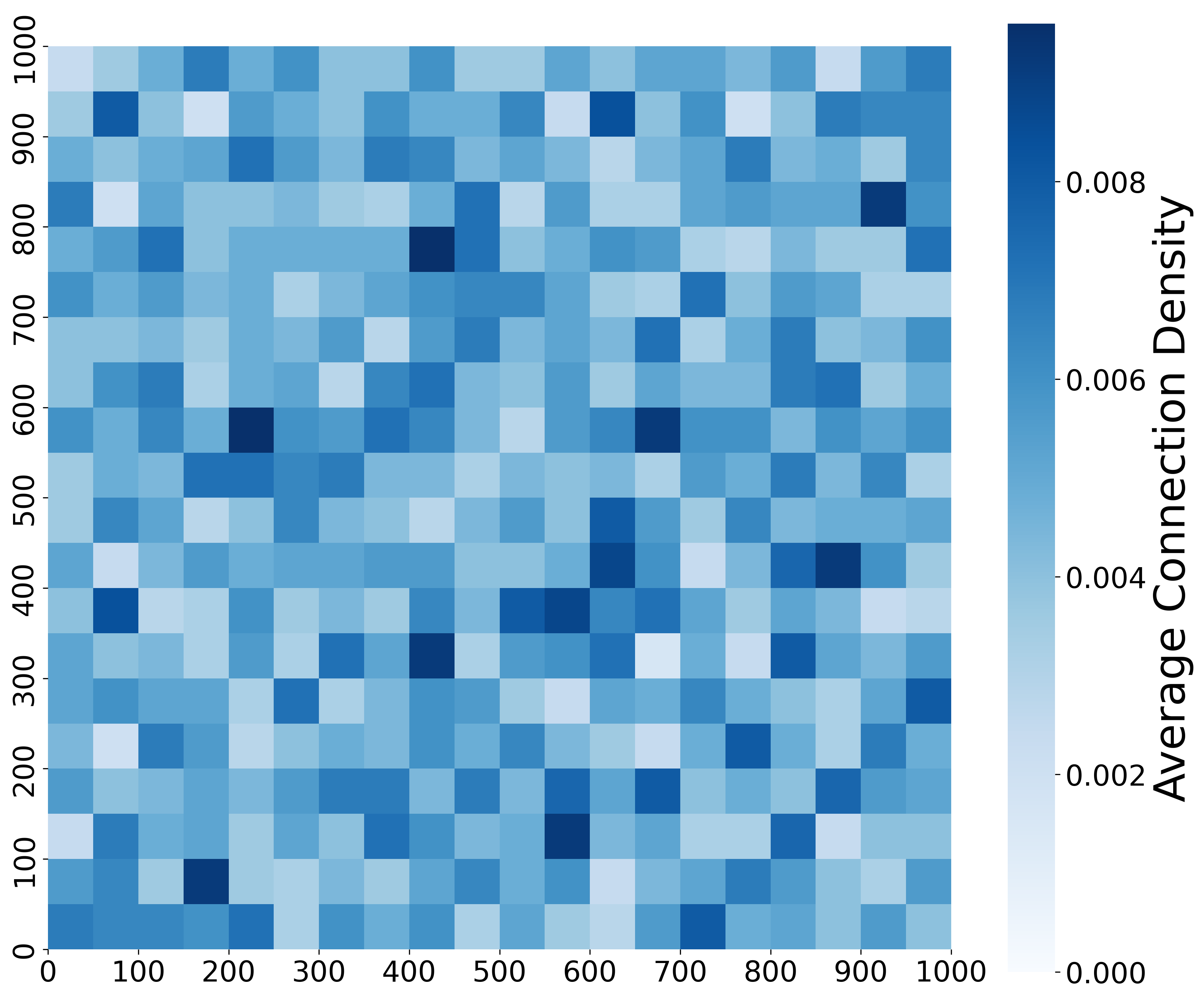
(a) Real topology $A$

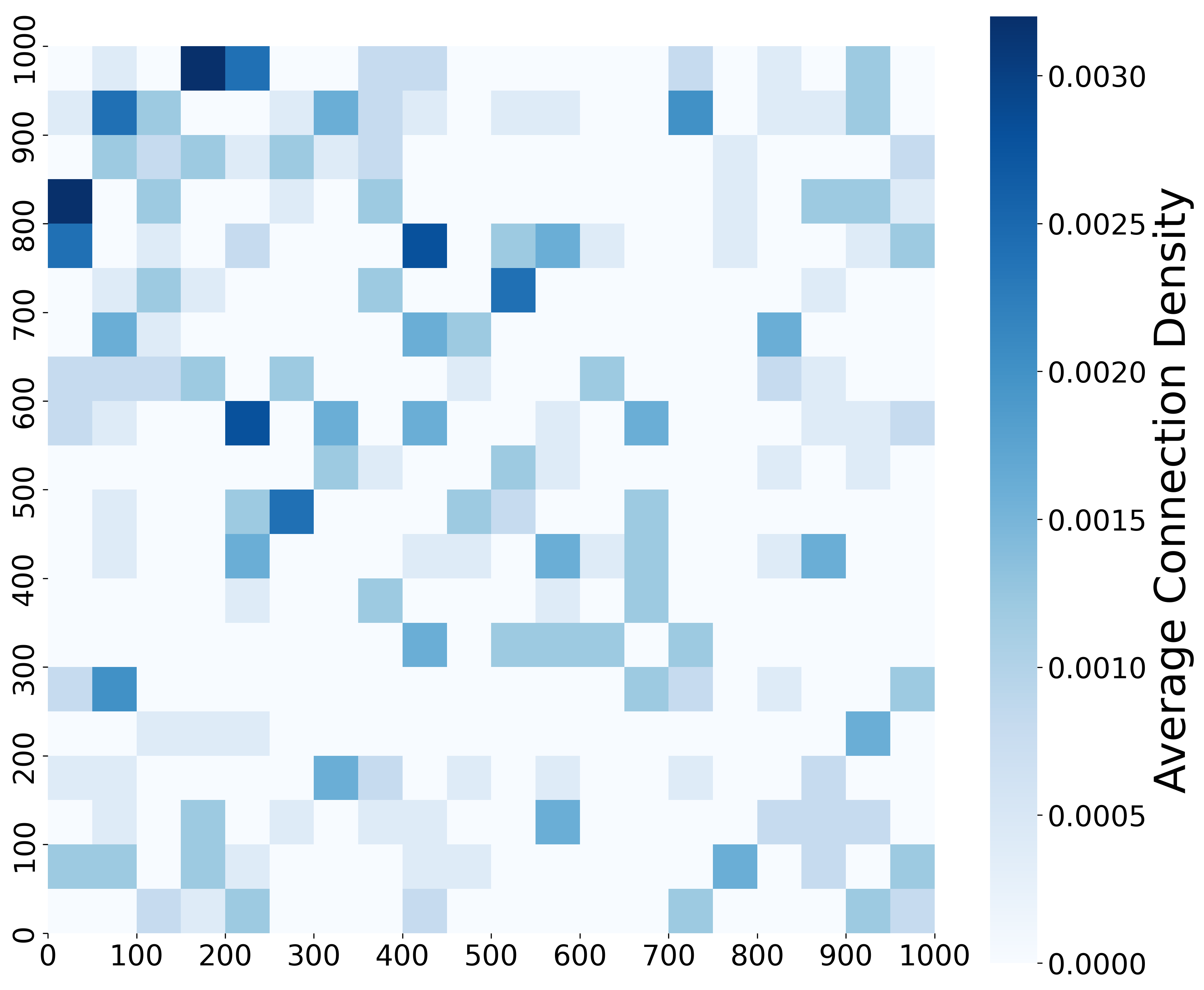
(b) $\Delta(A,A_{\text{Observed}})$

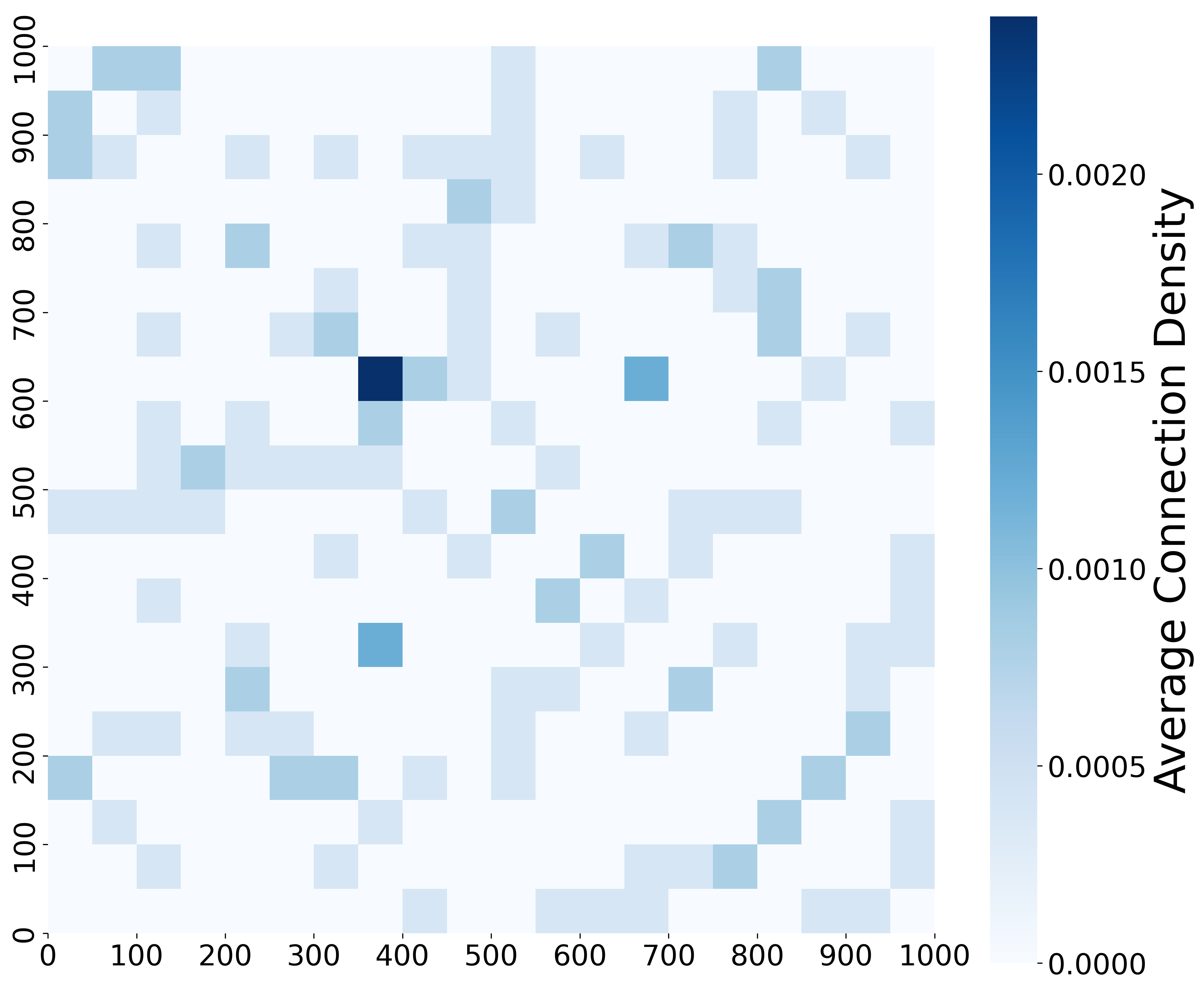
(c) $\Delta(A,\hat{A}_{\text{DeepNT}})$

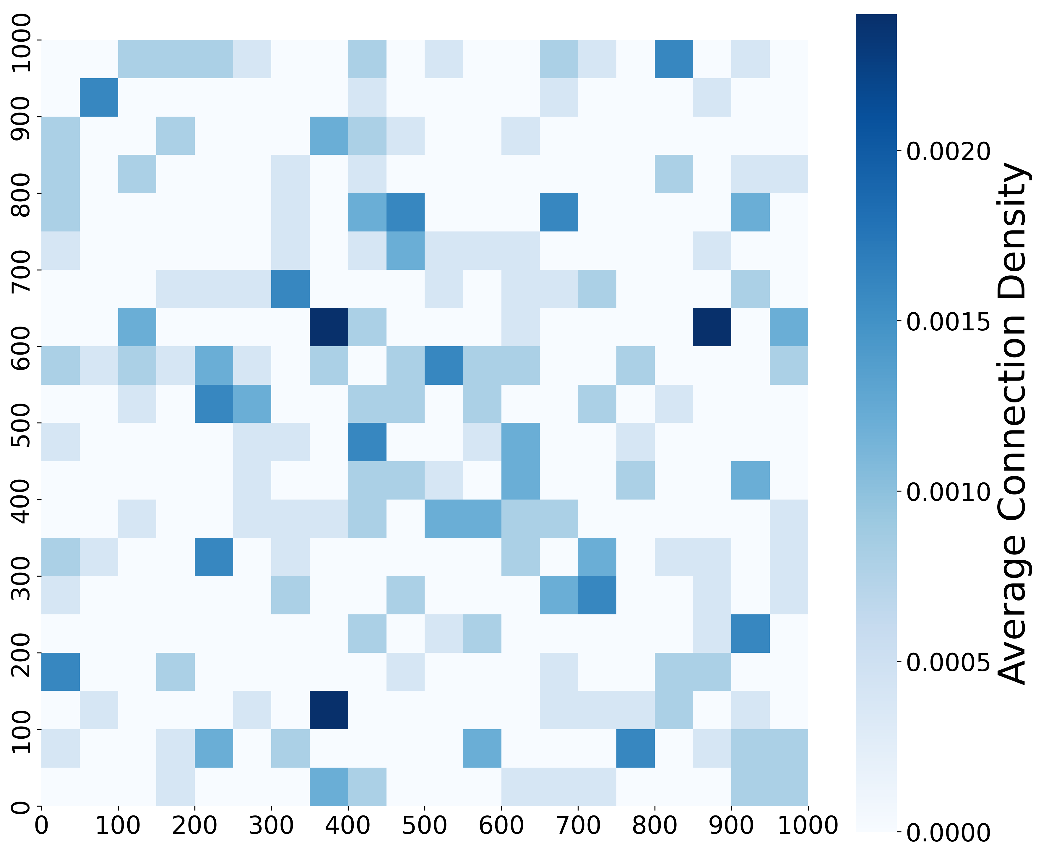
(d) $\Delta(A,\hat{A}_{\text{NeurTomography}})$

Figure 3. Heatmap of the real adjacency matrix and the difference ($\Delta$) between the real and learned adjacency matrices from various models for a synthetic network with 1,000 nodes and 2,521 edges, considering a topological error rate of 0.2 and path performance metrics, such as bandwidth.

As the network size increases, DeepNT shows superior scalability compared to the comparison models. For instance, for additional metrics on small datasets (e.g., the transportation dataset), comparison methods achieve comparable performance to DeepNT. At 10% sampling, NeuTomography achieves a MAPE of 0.6948, close to DeepNT’s 0.6342, while PAINT records a MAPE of 0.6508. This shows that on small networks, traditional models can be comparable to DeepNT. However, as the network size increases, such as on social network and Internet datasets, the performance gap between DeepNT and these comparison methods becomes obvious. On the Internet dataset at 30% sampling rate, DeepNT achieves a MAPE of 0.5842, while NeuTomography lags behind with a MAPE of 0.7276. PAINT only achieves a MAPE of 0.8108 on the same dataset.

5.2.2. Case Study of Network Topology Reconstruction

We further analyze the performance of network topology reconstruction given limited path information. We present a case study demonstrating the effectiveness of our proposed method for reconstructing network topology. For a network with 1,000 nodes and 2,521 edges with a topological error rate of 0.2, we visualize the heatmap of adjacency matrices where each block contains 50 nodes.

The path performance metric is the min/max metric, i.e., bandwidth, and $|S|/|T|=30\%$. As shown in Figure 3, DeepNT successfully recovers most of the true topology with minimal deviation in topology reconstruction. The heatmaps in Figure 3 demonstrate that the adjacency matrix learned by DeepNT is closer to the true adjacency matrix than the observed adjacency matrix and the adjacency matrix learned by NeuTomography. In particular, the denser and more complex parts of the network are more accurately recovered by DeepNT, which leads to smaller differences with the true adjacency matrix.

5.3. Ablation Study

To better understand how different components help our model predict various path performance metrics with incomplete network topology, we conduct ablation studies under different topology error rates $\Delta$ when $|S|/|T|=30\%$. There are two key predefined parameters, i.e., $\alpha$ and $\gamma$, which control the contributions for sparsity and path performance bounds, respectively. We set the value of one parameter to one and the others to zero, and examine how the performance changes to show the impact of each component.

Accordingly, two model variants, DeepNT-$\alpha$ and DeepNT-$\gamma$, are introduced. DeepNT-$\alpha$ sets $\alpha$ to $10^{-4}$ and $\gamma$ to 0, while DeepNT-$\gamma$ sets $\gamma$ to 1 and $\alpha$ to 0. We average the results of 500 Erdős-Rényi networks of the synthetic dataset for various tasks. Regression represents the average results for predicting additive, multiplicative, and min/max path performance metrics, while Classification reports the average results for predicting boolean path performance metrics. As shown in Table 5.3, when the sparsity ($\alpha$) or path performance bound ($\gamma$) constraints are removed, the performance significantly drops, demonstrating the importance of sparsity and boundary constraints under incomplete topological information. When the topology error rate $\Delta$ is small, DeepNT-$\gamma$ does not significantly improve the prediction performance. However, when $\Delta$ becomes larger, DeepNT-$\gamma$ (i.e., the path performance bound) can effectively reduce the impact of incorrect topology on prediction because it utilizes the possible correct path information to reconstruct the topology. Additionally, as $\Delta$ increases, the performance gap between DeepNT-$\alpha$ and DeepNT-$\gamma$ narrows, suggesting that maintaining sparsity in the adjacency matrix improves the model’s performance lower bound.

Table 5. Ablation study results.

$\Delta$	Method	Regression	Classification
		MAPE $\downarrow$	ACC $\uparrow$	$F_{1}$ $\uparrow$
10%	DeepNT	0.0741	0.8124	0.8043
2-5				DeepNT-$\alpha$	0.1236	0.6909	0.7341
2-5				DeepNT-$\gamma$	0.1014	0.7375	0.7582
20%	DeepNT	0.0852	0.7701	0.8041
2-5				DeepNT-$\alpha$	0.1305	0.6628	0.6733
2-5				DeepNT-$\gamma$	0.1187	0.7081	0.7336
30%	DeepNT	0.1129	0.7226	0.7636
2-5				DeepNT-$\alpha$	0.1368	0.6490	0.6827
2-5				DeepNT-$\gamma$	0.1212	0.6905	0.7294

One of the key components of this paper is the proposed path aggregation layer, which we compare with the information aggregation layers currently widely used in various graph neural networks. Detailed results can be found in the Appendix A.3. DeepNT with proposed path aggregation mechanism achieves the best performance for predicting additive metrics across most datasets.

6. Conclusion

In this paper, we introduce DeepNT, a novel framework for network tomography that addresses key challenges in predicting path performance metrics and network topology inference under incomplete and noisy observations. Through comprehensive experiments on real-world and synthetic datasets, DeepNT consistently outperforms state-of-the-art methods across a variety of path performance metrics, including additive, multiplicative, min/max, and boolean metrics. DeepNT demonstrates strong scalability and robustness, particularly as the network size and complexity increase, where traditional methods struggle to maintain performance.

Appendix A Appendix

A.1. Datasets

The statistics of the real-world datasets are shown in Table 6. For the initialization representation of nodes, if the source data already contains node features, we use them as the initialization node representations, otherwise we use binary encoding to convert the node identifier (e.g., node index) into a binary representation. For path performance metrics, we use the edge labels of the source data to generate the path labels. In addition, we generate random edge labels of other path performance metric types for some networks, and then generate the path labels. Path performance metrics of each dataset are shown in the Table 7.

Table 6. Dataset Statistics: the number of networks, (average) nodes and edges. $-$ indicates the dataset has a singe network.

Statistics	Internet		Social Network			Transportation
	IPV4	IPV6	Epinions	Twitter	Facebook	Anaheim	Winnipeg	Terrassa	Barcelona	Gold Cost
Graphs	10	10	-	-	-	-	-	-	-	-
1-11 Nodes	2866.0	1895.7	75,879	81,306	4,039	416	1,057	1,609	1,020	4,807
1-11 Edges	3119.6	2221.7	508,837	1768,149	88,234	914	2,535	3,264	2,522	11,140

Table 7. Properties of datasets. ✓ of binary encoding indicates that the original data has no node features, and we use binary encoding to generate the initial node representation. ✗ means that binary encoding is not used, but the node features of the original data are used. For the path performance metrics, ✓ for one metric indicates that the network has the true edge (link) labels of that metric, while ✓ indicates that random edge labels are generated for that performance metric.

Properties	Internet		Social Network			Transportation
	IPV4	IPV6	Epinions	Twitter	Facebook	Anaheim	Winnipeg	Terrassa	Barcelona	Gold Cost
Binary Enc.	✓	✓	✗	✗	✗	✓	✓	✓	✓	✓
Additive Path Performance Metrics
Delay			✓	✓	✓
1-11 RTT	✓	✓
1-11 Distance			✓	✓	✓
1-11 Flow Time						✓	✓	✓	✓	✓
Multiplicative Path Performance Metrics
Reliability	✓	✓
1-11 Trust Decay			✓	✓	✓
Min or Max Path Performance Metrics
Bandwidth	✓	✓
1-11 Capacity						✓	✓	✓	✓	✓
Boolean Path Performance Metrics
Is Trustworthy			✓
1-11 Is Secure						✓	✓	✓	✓	✓

For the synthetic dataset, we utilize the Erdos-Renyi algorithm to generate networks of different sizes. Then, we generate random edge labels for all the above path performance metrics. When generating random edge labels for all datasets, for the addition and min/max metrics, the random labels are in $[1,100]$, and for the multiplication metric, the random labels are in $[0.9,0.999]$. For the Boolean metrics, each edge is randomly assigned a state of 0 or 1, where path labels are controlled to be balanced (the number of positive and negative labels will not less than 30%).

A.2. Implementation

The training data for each dataset depends on the sampling rate, i.e., $\frac{|S|}{|T|}$ which indicates how many node pairs’ end-to-end path performance metric values are used for training. Half of node pairs in $S$ is used as training data, and the other half is used as the validation set. That is, the number of node pairs actually used as training data is $\frac{|S|}{2}$. The rest of node pairs in $T\setminus S$ are used as test data.

To train DeepNT, we use CrossEntropyLoss as the loss function for classification tasks (Boolean metric) and MSELoss as the loss function for regression tasks (additive, multiplicative, and min/max metrics). Adam optimizer is used to optimize the model. The learning rate is set to 1e-4 across all tasks and models. The training batch is set to 1024 and the test batch is 2048 for all datasets. We use GCN as the GNN backbone, and the number of layers of GCN is 2. We use the mean pooling as the READOUT function. An one-layer MLP is used to make predictions. All models are trained for a maximum of 500 epochs using an early stop scheme with the patience of 10. The hidden dimension is set to 256. The hyperparameters we tune include the number of sampled shortest paths $N$ in 1, 2, 3, the sparsity parameter $\alpha$ in 10e-5, 10e-4, 10e-3, 10e-2, and the path performance bound parameter $\gamma$ in 0.1, 0.25, 0.5, 1, 2, 4, 8, 16.

For the comparison methods, we follow the original settings provided by the authors. In particular, the ANMI threshold ratio is reported as 30%. AMPR requires multiple probe tests, and we set the number of probe tests to the number of placed monitors, since each monitor tests the end-to-end path performance with other nodes.

A.3. Ablation Study on information aggregation

We compare our path aggregation with aggregation operations from SEAL (subgraph aggregation) (Zhang and Chen, 2018), LESSR (edge-order preserving aggregation) (Chen and Wong, 2020), PNA (principal neighborhood aggregation) (Corso et al., 2020), and OSAN (ordered subgraph aggregation) (Qian et al., 2022). A brief description of these aggregation methods is provided in Table 9.

The results in Table 8 demonstrate that the path aggregation mechanism in DeepNT achieves the lowest MSE for predicting additive metrics across most datasets, outperforming alternative aggregation methods. This suggests that path-specific attention effectively captures the most probable paths with optimal performance, leading to finer-grained and more accurate network tomography. Edge-order preserving aggregation performs best in the transportation dataset, likely due to its ability to preserve sequential dependencies in structured paths. However, in other cases, subgraph and ordered subgraph aggregation methods exhibit higher errors, indicating that local subgraph representations alone may not be sufficient for capturing global path information required in network tomography.

Table 8. MSE results using different aggregation layers.

DeepNT	Internet	Social	Transportation	Synthetic
w/ subgraph	117.65	22.90	21.77	77.93
w/ edge-order	84.25	14.19	17.11	62.65
w/ principal	94.43	20.01	22.89	84.07
w/ ordered subg.	101.73	17.26	20.57	71.14
w/ path (ours)	71.08	10.81	18.66	59.04

Table 9. Comparison of different graph aggregation models.

Model	Formula	Description
DeepNT	$\hat{h}_{v}^{(n)}=h_{v}+\sigma\left(\sum_{x\in\mathcal{P}_{vu}^{(n)}}\alpha_{vx}^{(n)}h_{x}^{(n)}\right)$	Path aggregation: Aggregates over sampled optimal paths.
	$\alpha_{vx}^{(n)}=\operatorname{softmax}(r^{T}[h_{v},h_{x}^{(n)}])$
	$h_{v}=\operatorname{READOUT}(\hat{h}_{v}^{(n)}\cdot P_{vu}^{(n)}\subset P_{vu}^{L})$
SEAL	$h_{v}=\operatorname{AGG}(h_{v}:v\in G_{h}^{x,y})$	Subgraph aggregation: Aggregates node features within en-
	$h_{vp}=\operatorname{READOUT}(h_{v}:G_{h}^{x,y}\in\text{enclosing subgraphs})$	closing subgraphs extracted for target links.
LESSR	$h_{v}=\operatorname{GRU}(h_{v},h_{z}:z\in\mathcal{N}(v))$	Edge-order preserving aggregation: Combines GRU-based
	$h_{vp}=\operatorname{Attention}(h_{v},h_{x},\text{shortcut connections})$	local aggregation with global attention from shortcut paths.
	$h_{v}=\operatorname{READOUT}(\operatorname{EOPA}(h_{v}),\operatorname{SGAT}(h_{v}))$
PNA	$h_{agg}=\operatorname{AGG}(h_{u}:u\in\mathcal{N}(v))$	Principal neighbourhood aggregation: Combines mean,
	$h_{\text{scaled}}=\operatorname{Scaler}(\operatorname{deg}(v))\cdot h_{\text{agg}}$	max, min, and std aggregators with degree-based scaling.
	$h_{v}=\operatorname{Combine}(h_{\text{scaled}})$
OSAN	$h_{s}=\operatorname{AGG}(f_{w}(v):v\in s)$	Ordered subgraph aggregation: Aggregates features from
	$h_{v}=\operatorname{READOUT}(h_{s}:v\in s,s\in S)$	WL-labeled subgraphs containing the node.

A.4. Expressiveness Study

A path from a source node $v$ to a target node $u$ is denoted by $p_{uv}=[v_{1},v_{2},\dots,v_{k}]$, where $v_{1}=v$, $v_{k}=u$, and $(v_{i},v_{i+1})\in E$ for $i\in\{1,\dots,k-1\}$. Paths contain distinct vertices, and the length of the path is given by $|p_{uv}|=k-1$, defined as the number of edges it contains. In this work, we consider paths that adhere to these criteria.

In practice, we only consider paths up to a fixed length $L$. Let $\mathcal{P}_{uv}^{L}$ denote the set of the sampled top-$N$ optimal paths from $u$ to $v$, selected based on the best path performance, with lengths not exceeding $L$. Recall that $S$ and $T$ represent the set of node pairs with observed path performance and all possible node pairs, respectively. Define $\mathcal{SP}=\bigcup_{<u,v>\in S}\mathcal{P}_{uv}^{L}$ as the collection of all sampled paths, and let $\mathcal{AP}$ denote the collection of all paths between the node pair combinations in $T$. We have $\mathcal{P}_{uv}^{L}\subset\mathcal{SP}\subseteq\mathcal{AP}$, where $\mathcal{SP}\to\mathcal{AP}$ as $N\to\infty$ and $S\to T$. To strengthen the proof, we first introduce the concepts of WL-Tree and Path-Tree as defined by Michel et al..

Definition A.1 (WL-Tree rooted at $v$).

Let $G=(V,E)$. A WL-Tree $W_{v}^{L}$ is a tree rooted at node $v\in V$ encoding the structural information captured by the 1-WL algorithm up to $L$ iterations. At each iteration, the children of a node $u$ are its direct neighbors, $\mathcal{N}(u)=\{w\mid(u,w)\in E\}$.

Definition A.2 (Path-Tree rooted at $v$).

Let $G=(V,E)$. A Path-Tree $P_{v}^{L}$ rooted at a node $v\in V$ is a tree of height $L$, where the node set at level $k$ is the multiset of nodes that appear at position $k$ in the paths of $\mathcal{P}_{v}^{L}$, i.e., $\{u\mid p^{L}(k)=u\text{ for }p^{L}\in\mathcal{P}_{v}^{L}\}.$ Nodes at level $k$ and level $k+1$ are connected if and only if they occur in adjacent positions $k$ and $k+1$ in any path $p^{L}\in\mathcal{P}_{v}^{L}$.

Theorem A.3 (DeepNT-$\mathcal{AP}$ Expressiveness Beyond 1-WL).

Let $G=(V,E)$, $W_{v}^{L}$ and $W_{u}^{L}$ denote the WL-Trees of height $L$ rooted at nodes $v,u\in V$, respectively. Let $f_{\text{DeepNT}}(v)$ and $f_{\text{DeepNT}}(u)$ represent the embeddings produced by DeepNT when it has access to the complete set of paths $\mathcal{AP}$. Then the following holds:

1. If $W_{v}^{L}\neq W_{u}^{L}$, then $f_{\text{DeepNT}}(v)\neq f_{\text{DeepNT}}(u)$.

2. If $W_{v}^{L}=W_{u}^{L}$, it is still possible that $f_{\text{DeepNT}}(v)\neq f_{\text{DeepNT}}(u)$.

Proof.

To prove this statement, we refer to Theorem 3.3 from (Michel et al., 2023), which states that if $W_{v}^{L}$ is structurally different from $W_{u}^{L}$ (i.e., not isomorphic), then $P_{v}^{L}$ is also structurally different from $P_{u}^{L}$. Moreover, $P_{v}^{L}$ and $P_{u}^{L}$ can still differ even if $W_{v}^{L}$ and $W_{u}^{L}$ are identical.

We first address the case where $W_{v}^{L}\neq W_{u}^{L}$. It follows that $P_{v}^{L}$ and $P_{u}^{L}$ will not be isomorphic. The path aggregation layer in DeepNT is straightforward to prove as injective, as it employs a permutation-invariant readout function. Consequently, DeepNT aggregates path-centric structural information from $P_{v}^{L}$ and $P_{u}^{L}$ to produce embeddings $f_{\text{DeepNT}}(v)$ and $f_{\text{DeepNT}}(u)$, which are guaranteed to be distinct.

Now consider the case where $W_{v}^{L}=W_{u}^{L}$. This implies that 1-WL cannot distinguish between $v$ and $u$. However, $P_{v}^{L}$ and $P_{u}^{L}$ may still differ. The path aggregation layer of DeepNT captures path-centric structural information from $P_{v}^{L}$ and $P_{u}^{L}$, resulting in distinct embeddings $f_{\text{DeepNT}}(v)$ and $f_{\text{DeepNT}}(u)$. Thus, DeepNT surpasses the expressiveness of 1-WL. This completes the proof. ∎

Finally, Theorem 4.1 can be readily proved by noting that the node pairs $\langle u,v\rangle$ and $\langle u^{\prime},v^{\prime}\rangle$ are represented by concatenated node embeddings. Since $\mathcal{P}_{uv}^{L}\neq\mathcal{P}_{u^{\prime}v^{\prime}}^{L}$, the distinctiveness of these representations is ensured by the expressive power of DeepNT, which surpasses that of 1-WL.

A.5. Proof of Theorem 4.2

Proof.

For the weak connectivity of the entire graph, following Zhao et al., we show that for any nonzero vector $x\in\mathbb{R}^{|V|}$:

$$x^{\top}Z_{G}x=\sum_{i\neq j}A_{ij}(x_{i}-x_{j})^{2}+\frac{1}{|V|}\left(\sum_{i=1}^{|V|}x_{i}\right)^{2}>0.$$

The first term ensures that differences between connected nodes contribute positively, while the rank-1 term $\frac{1}{|V|}\left(\sum_{i=1}^{|V|}x_{i}\right)^{2}$ prevents the existence of isolated components when edge directions are ignored. This guarantees that the graph $G$ is weakly connected.

For strong connectivity within each component $g\in\mathcal{G}$, we establish both necessity and sufficiency. For necessity, if $g$ is strongly connected, then its adjacency submatrix $A_{g}$ is irreducible by the Perron–Frobenius theorem, implying that $A_{g}+A_{g}^{\top}$ provides bidirectional coupling between any partition of nodes in $g$. Combined with the positive diagonal terms $\operatorname{diag}(A_{g}\cdot\mathbf{1}^{\top})+\operatorname{diag}(A_{g}^{\top}\cdot\mathbf{1}^{\top})$ and the rank-1 term $2\left(\frac{1}{|g|}\mathbf{1}\mathbf{1}^{\top}\right)$, this ensures $Z_{g}+Z_{g}^{\top}\succ 0$.

For sufficiency, we prove by contradiction. If $g$ were not strongly connected, then $A_{g}$ would be permutable to a block upper-triangular form as $A_{g}=\begin{pmatrix}A_{11}&A_{12}\\ 0&A_{22}\end{pmatrix},$ where $A_{11}$ and $A_{22}$ correspond to disconnected subcomponents. We could construct a nonzero vector $y$ conforming to these blocks such that $y^{\top}(Z_{g}+Z_{g}^{\top})y=0$, contradicting the positive definiteness of $Z_{g}+Z_{g}^{\top}$. Therefore, $Z_{g}+Z_{g}^{\top}\succ 0$ if and only if $g$ is strongly connected. This completes the proof. ∎

A.6. Proof of Theorem 4.3

Proof Sketch.

The coercivity of the objective function $g(\theta,\tilde{A})+\alpha\|\tilde{A}\|_{1}$ ensures that the sequence $\{(\theta^{k},\tilde{A}^{k})\}$ is bounded. By the Bolzano–Weierstrass theorem, there exists at least one limit point $(\theta^{*},\tilde{A}^{*})$ (Wen et al., 2017). Since the step size satisfies $\frac{1}{L}\leq\omega\leq\sqrt{\frac{L}{L+l}}$, the function sequence $\{\mathcal{F}(\theta^{k},\tilde{A}^{k})\}$ is non-increasing and converges to a finite value. The proximal gradient updates ensure $\|\nabla g(\theta^{k+1},\tilde{A}^{k+1})-\nabla g(\theta^{k},\tilde{A}^{k})\|\to 0$, implying that the gradients converge. Taking the limit of the update steps, we obtain $\nabla_{\theta}g(\theta^{*},\tilde{A}^{*})=\mathbf{0}$, and the optimality condition for $\tilde{A}$ satisfies $\mathbf{0}\in\nabla_{\tilde{A}}g(\theta^{*},\tilde{A}^{*})+\alpha\partial\|\tilde{A}^{*}\|_{1}$. Since every limit point of $\{(\theta^{k},\tilde{A}^{k})\}$ satisfies these conditions, the sequence converges to a stationary point, completing the proof. ∎

Proof.

With the chosen step size satisfying $\frac{1}{L}\leq\omega\leq\sqrt{\frac{L}{L+l}}$, the proximal gradient algorithm ensures:

$$\mathcal{F}(\theta^{k+1},\tilde{A}^{k+1})\leq\mathcal{F}(\theta^{k},\tilde{A}^{k}).$$

This implies that the sequence $\{\mathcal{F}(\theta^{k},\tilde{A}^{k})\}$ is non-increasing. Since $\mathcal{F}(\theta,\tilde{A})$ is bounded below (due to the coercivity of the $\ell_{1}$-regularization term $\alpha\|\tilde{A}\|_{1}$), the sequence $\{\mathcal{F}(\theta^{k},\tilde{A}^{k})\}$ converges to a finite value.

The boundedness of $\mathcal{F}(\theta^{k},\tilde{A}^{k})$ ensures that the sequence $\{(\theta^{k},\tilde{A}^{k})\}$ is bounded, which means $\{(\theta^{k},\tilde{A}^{k})\}$ has at least one limit point $(\theta^{*},\tilde{A}^{*})$.

Since $\|(\theta^{k+1},\tilde{A}^{k+1})-(\theta^{k},\tilde{A}^{k})\|\to 0$, and $\nabla g$ is Lipschitz continuous, it follows that:

$$\|\nabla g(\theta^{k+1},\tilde{A}^{k+1})-\nabla g(\theta^{k},\tilde{A}^{k})\|\to 0.$$

Therefore, the gradients $\nabla g(\theta^{k},\tilde{A}^{k})$ converge to $\nabla g(\theta^{*},\tilde{A}^{*})$ as $k\to\infty$.

The update for $\theta$ in Algorithm 1 is:

$$\theta^{k+1}-\overline{\theta}^{k}=-\omega\nabla_{\theta}g(\overline{\theta}^{k},\overline{A}^{k}).$$

As $k\to\infty$, $\overline{\theta}^{k}\to\theta^{*}$, $\theta^{k+1}-\overline{\theta}^{k}\to 0$ and $\nabla_{\theta}g(\overline{\theta}^{k},\overline{A}^{k})\to\nabla_{\theta}g(\theta^{*},\tilde{A}^{*})$. Then, it follows that:

$$\nabla_{\theta}g(\theta^{*},\tilde{A}^{*})=\mathbf{0}.$$

The update for $\tilde{A}$ in Algorithm 1 involves solving the proximal operator:

$$\tilde{A}^{k+1}=\arg\min_{\tilde{A}}\left(\frac{1}{2}\left\|\tilde{A}-\left(\overline{A}^{k}-\omega\nabla_{\tilde{A}}g(\overline{\theta}^{k},\overline{A}^{k})\right)\right\|_{F}^{2}+\omega\alpha\|\tilde{A}\|_{1}\right).$$

This optimization is equivalent to applying the proximal mapping:

$$\tilde{A}^{k+1}=\operatorname{prox}_{\omega\alpha\|\cdot\|_{1}}\left(\overline{A}^{k}-\omega\nabla_{\tilde{A}}g(\overline{\theta}^{k},\overline{A}^{k})\right),$$

where $\operatorname{prox}_{\lambda\|\cdot\|_{1}}(f)=S_{\lambda}(f)$ is the soft-thresholding operator. The proximal mapping satisfies the optimality condition:

$$\mathbf{0}\in\tilde{A}^{k+1}-\left(\overline{A}^{k}-\omega\nabla_{\tilde{A}}g(\overline{\theta}^{k},\overline{A}^{k})\right)+\omega\alpha\partial\|\tilde{A}^{k+1}\|_{1}.$$

Rearranging this condition gives:

$$\mathbf{0}\in\nabla_{\tilde{A}}g(\overline{\theta}^{k},\overline{A}^{k})+\frac{1}{\omega}(\tilde{A}^{k+1}-\overline{A}^{k})+\alpha\partial\|\tilde{A}^{k+1}\|_{1}.$$

As $k\to\infty$, the extrapolated sequence $\overline{A}^{k}\to\tilde{A}^{*}$ and the proximal updates $\tilde{A}^{k+1}\to\tilde{A}^{*}$. Consequently, the term $(\tilde{A}^{k+1}-\overline{A}^{k})/\omega\to\mathbf{0}$. Thus, the limit point $\tilde{A}^{*}$ satisfies:

$$\mathbf{0}\in\nabla_{\tilde{A}}g(\theta^{*},\tilde{A}^{*})+\alpha\partial\|\tilde{A}^{*}\|_{1}.$$

We conclude that $(\theta^{*},\tilde{A}^{*})$ is a stationary point of the optimization problem since both optimality conditions are satisfied:

$$\mathbf{0}\in\nabla_{\theta}g(\theta^{*},\tilde{A}^{*}),\quad\mathbf{0}\in\nabla_{\tilde{A}}g(\theta^{*},\tilde{A}^{*})+\alpha\partial\|\tilde{A}^{*}\|_{1}.$$

The algorithm may adjust $\tilde{A}^{k+1}$ to ensure connectivity. This adjustment does not violate convergence guarantees because it is a bounded perturbation that preserves the descent property.

Therefore, the sequence $\{(\theta^{k},\tilde{A}^{k})\}$ converges to the stationary point $(\theta^{*},\tilde{A}^{*})$: $\lim_{k\to\infty}(\theta^{k},\tilde{A}^{k})=(\theta^{*},\tilde{A}^{*}).$ This establishes the convergence of the algorithm and completes the proof.

∎

A.7. Proof of Theorem 4.4

Proof.

As $N\to\infty$, the sampled paths $\mathcal{SP}$ converge to the complete set of paths for the observed node pairs $S$. As $S\to T$, the set of observed node pairs expands to include all possible node pairs in $T=V\times V$. Therefore, $\mathcal{SP}\to\mathcal{AP}$ as $N\to\infty$ and $S\to T$, which means DeepNT-$\mathcal{SP}$ converges to DeepNT-$\mathcal{AP}$.

By Theorem A.3 (DeepNT-$\mathcal{AP}$ Expressiveness Beyond 1-WL) and Theorem 4.1 (DeepNT-$\mathcal{AP}$ Distinguishes Node Pairs Beyond 1-WL), DeepNT-$\mathcal{AP}$ can uniquely identify and distinguish all node pairs based on differences in their path sets. Moreover, by Theorem 4.3 (Convergence of DeepNT’s Optimization), the optimization of DeepNT converges to a stationary point $(\theta^{*},\tilde{A}^{*})$. This ensures that the empirical loss over the observed pairs $S$ is minimized:

$$\mathcal{L}(\theta^{*},\tilde{A}^{*})=\sum_{\langle u,v\rangle\in S}l(f_{\text{DeepNT}}(u,v;\theta^{*},\tilde{A}^{*}),y_{uv}),$$

where $l(\cdot,\cdot)$ measures the error between the predicted metrics $\hat{y}_{uv}$ and the true metrics $y_{uv}$. Consequently, as $S\to T$, the training error diminishes:

$$\mathbb{E}_{\langle u,v\rangle\sim S}[\lvert\hat{y}_{uv}-y_{uv}\rvert]\to 0.$$

As $S\to T$, the observed set $S$ becomes dense, covering all node pairs in $T=V\times V$. Therefore, the unobserved set $T\setminus S$ becomes empty, i.e., $T\setminus S\to\emptyset$. Combined with the expressiveness of DeepNT and the completeness of path sampling, the model generalizes well to unobserved pairs $\langle u,v\rangle\in T\setminus S$. This ensures that the generalization error also diminishes:

$$\mathbb{E}_{\langle u,v\rangle\sim T\setminus S}[\lvert\hat{y}_{uv}-y_{uv}\rvert]\to 0.$$

Combining these results, the total error for all node pairs in $T$, which is the sum of the training error and the generalization error, converges to zero:

$$\epsilon_{\text{total}}=\mathbb{E}_{\langle u,v\rangle\sim S}[\lvert\hat{y}_{uv}-y_{uv}\rvert]+\mathbb{E}_{\langle u,v\rangle\sim T\setminus S}[\lvert\hat{y}_{uv}-y_{uv}\rvert]\to 0.$$

Finally, as $N\to\infty$ and $S\to T$, DeepNT-$\mathcal{SP}$ converges to DeepNT-$\mathcal{AP}$, and the predicted metrics $\hat{y}_{uv}$ converge in expectation to the true metrics $y_{uv}$:

$$\lim_{S\to T}\lim_{N\to\infty}\mathbb{E}_{\langle u,v\rangle\sim T}\left[\lvert\hat{y}_{uv}-y_{uv}\rvert\right]=0.$$

This completes the proof. ∎

References

- (1)
- Alon et al. (2014) Noga Alon, Yuval Emek, Michal Feldman, and Moshe Tennenholtz. 2014. Economical graph discovery. Operations Research 62, 6 (2014), 1236–1246.
- Bartolini et al. (2020) Novella Bartolini, Ting He, Viviana Arrigoni, Annalisa Massini, Federico Trombetti, and Hana Khamfroush. 2020. On fundamental bounds on failure identifiability by boolean network tomography. IEEE/ACM Transactions on Networking 28, 2 (2020), 588–601.
- Bejerano and Rastogi (2003) Yigal Bejerano and Rajeev Rastogi. 2003. Robust monitoring of link delays and faults in IP networks. In IEEE INFOCOM 2003. Twenty-second Annual Joint Conference of the IEEE Computer and Communications Societies (IEEE Cat. No. 03CH37428), Vol. 1. IEEE, 134–144.
- Bu et al. (2002) Tian Bu, Nick Duffield, Francesco Lo Presti, and Don Towsley. 2002. Network tomography on general topologies. ACM SIGMETRICS Performance Evaluation Review 30, 1 (2002), 21–30.
- Candes and Recht (2012) Emmanuel Candes and Benjamin Recht. 2012. Exact matrix completion via convex optimization. Commun. ACM 55, 6 (2012), 111–119.
- Cao and Sun (2012) Yue Cao and Zhili Sun. 2012. Routing in delay/disruption tolerant networks: A taxonomy, survey and challenges. IEEE Communications surveys & tutorials 15, 2 (2012), 654–677.
- Carter and Crovella (1996) Robert L Carter and Mark E Crovella. 1996. Measuring bottleneck link speed in packet-switched networks. Performance evaluation 27 (1996), 297–318.
- Chen et al. (2010) Aiyou Chen, Jin Cao, and Tian Bu. 2010. Network tomography: Identifiability and fourier domain estimation. IEEE Transactions on Signal Processing 58, 12 (2010), 6029–6039.
- Chen et al. (2018) Lu Chen, Bowen Tan, Sishan Long, and Kai Yu. 2018. Structured dialogue policy with graph neural networks. In Proceedings of the 27th International Conference on Computational Linguistics. 1257–1268.
- Chen and Wong (2020) Tianwen Chen and Raymond Chi-Wing Wong. 2020. Handling information loss of graph neural networks for session-based recommendation. In Proceedings of the 26th ACM SIGKDD international conference on knowledge discovery & data mining. 1172–1180.
- Chen et al. (2003) Yan Chen, David Bindel, and Randy H Katz. 2003. Tomography-based overlay network monitoring. In Proceedings of the 3rd ACM SIGCOMM conference on Internet measurement. 216–231.
- Chen et al. (2020a) Yu Chen, Lingfei Wu, and Mohammed Zaki. 2020a. Iterative deep graph learning for graph neural networks: Better and robust node embeddings. Advances in neural information processing systems 33 (2020), 19314–19326.
- Chen et al. (2020b) Yu Chen, Lingfei Wu, and Mohammed J Zaki. 2020b. Reinforcement Learning Based Graph-to-Sequence Model for Natural Question Generation. In International Conference on Learning Representations.
- Chorowski et al. (2015) Jan K Chorowski, Dzmitry Bahdanau, Dmitriy Serdyuk, Kyunghyun Cho, and Yoshua Bengio. 2015. Attention-based models for speech recognition. Advances in neural information processing systems 28 (2015).
- Chua et al. (2005) David B Chua, Eric D Kolaczyk, and Mark Crovella. 2005. Efficient monitoring of end-to-end network properties. In Proceedings IEEE 24th Annual Joint Conference of the IEEE Computer and Communications Societies., Vol. 3. IEEE, 1701–1711.
- Corso et al. (2020) Gabriele Corso, Luca Cavalleri, Dominique Beaini, Pietro Liò, and Petar Veličković. 2020. Principal neighbourhood aggregation for graph nets. Advances in Neural Information Processing Systems 33 (2020), 13260–13271.
- Duffield (2003) Nick Duffield. 2003. Simple network performance tomography. In Proceedings of the 3rd ACM SIGCOMM conference on Internet measurement. 210–215.
- Duffield (2006) Nick Duffield. 2006. Network tomography of binary network performance characteristics. IEEE Transactions on Information Theory 52, 12 (2006), 5373–5388.
- Fan and Li (2017) XiaoBo Fan and Xingming Li. 2017. Network tomography via sparse Bayesian learning. IEEE Communications Letters 21, 4 (2017), 781–784.
- Feng et al. (2020) Cuiying Feng, Luning Wang, Kui Wu, and Jianping Wang. 2020. Bound inference in network performance tomography with additive metrics. IEEE/ACM Transactions on Networking 28, 4 (2020), 1859–1871.
- Firooz and Roy (2010) Mohammad H Firooz and Sumit Roy. 2010. Network tomography via compressed sensing. In 2010 IEEE Global Telecommunications Conference GLOBECOM 2010. IEEE, 1–5.
- Franceschi et al. (2019) Luca Franceschi, Mathias Niepert, Massimiliano Pontil, and Xiao He. 2019. Learning discrete structures for graph neural networks. In International conference on machine learning. PMLR, 1972–1982.
- Galesi and Ranjbar (2018) Nicola Galesi and Fariba Ranjbar. 2018. Tight Bounds for Maximal Identifiability of Failure Nodes in Boolean Network Tomography. In 2018 IEEE 38th International Conference on Distributed Computing Systems (ICDCS). 212–222. https://doi.org/10.1109/ICDCS.2018.00030
- Gopalan and Ramasubramanian (2011) Abishek Gopalan and Srinivasan Ramasubramanian. 2011. On identifying additive link metrics using linearly independent cycles and paths. IEEE/ACM Transactions on Networking 20, 3 (2011), 906–916.
- Gurewitz and Sidi (2001) Omer Gurewitz and Moshe Sidi. 2001. Estimating one-way delays from cyclic-path delay measurements. In Proceedings IEEE INFOCOM 2001. Conference on Computer Communications. Twentieth Annual Joint Conference of the IEEE Computer and Communications Society (Cat. No. 01CH37213), Vol. 2. IEEE, 1038–1044.
- He (2018) Ting He. 2018. Distributed Link Anomaly Detection via Partial Network Tomography. SIGMETRICS Perform. Eval. Rev. 45, 3 (mar 2018), 29–42.
- He et al. (2017) Xiangnan He, Lizi Liao, Hanwang Zhang, Liqiang Nie, Xia Hu, and Tat-Seng Chua. 2017. Neural collaborative filtering. In Proceedings of the 26th international conference on world wide web. 173–182.
- Horton and López-Ortiz (2003) Joseph D Horton and Alejandro López-Ortiz. 2003. On the number of distributed measurement points for network tomography. In Proceedings of the 3rd ACM SIGCOMM conference on Internet measurement. 204–209.
- Ibraheem et al. (2023) Amani Ibraheem, Zhengguo Sheng, George Parisis, and Daxin Tian. 2023. Network Tomography-based Anomaly Detection and Localisation in Centralised In-Vehicle Network. In 2023 IEEE International Conference on Omni-layer Intelligent Systems (COINS). IEEE, 1–6.
- Ikeuchi et al. (2022) Hiroki Ikeuchi, Hiroshi Saito, and Kotaro Matsuda. 2022. Network tomography based on adaptive measurements in probabilistic routing. In IEEE INFOCOM 2022-IEEE Conference on Computer Communications. IEEE, 2148–2157.
- Jain and Dovrolis (2002) Manish Jain and Constantinos Dovrolis. 2002. End-to-end available bandwidth: Measurement methodology, dynamics, and relation with TCP throughput. ACM SIGCOMM Computer Communication Review 32, 4 (2002), 295–308.
- Jin et al. (2020) Wei Jin, Yao Ma, Xiaorui Liu, Xianfeng Tang, Suhang Wang, and Jiliang Tang. 2020. Graph structure learning for robust graph neural networks. In Proceedings of the 26th ACM SIGKDD international conference on knowledge discovery & data mining. 66–74.
- Kazemi et al. (2020) Seyed Mehran Kazemi, Rishab Goel, Kshitij Jain, Ivan Kobyzev, Akshay Sethi, Peter Forsyth, and Pascal Poupart. 2020. Representation learning for dynamic graphs: A survey. J. Mach. Learn. Res. 21, 70 (2020), 1–73.
- Kompella et al. (2007) Ramana Rao Kompella, Jennifer Yates, Albert Greenberg, and Alex C Snoeren. 2007. Detection and localization of network black holes. In IEEE INFOCOM 2007-26th IEEE International Conference on Computer Communications. IEEE, 2180–2188.
- Lai and Baker (2000) Kevin Lai and Mary Baker. 2000. Measuring link bandwidths using a deterministic model of packet delay. In Proceedings of the conference on applications, technologies, architectures, and protocols for computer communication. 283–294.
- Lee and Seung (2000) Daniel Lee and H Sebastian Seung. 2000. Algorithms for non-negative matrix factorization. Advances in neural information processing systems 13 (2000).
- Lev-Ari et al. (2023) Hanoch Lev-Ari, Yariv Ephraim, and Brian L Mark. 2023. Traffic rate network tomography with higher-order cumulants. Networks 81, 2 (2023), 220–234.
- Li et al. (2023) Huikang Li, Yi Gao, Wei Dong, and Chun Chen. 2023. Bound-Based Network Tomography for Inferring Interesting Path Metrics. IEEE/ACM Transactions on Networking 31, 01 (2023), 1–14.
- Liang and Yu (2003) Gang Liang and Bin Yu. 2003. Maximum pseudo likelihood estimation in network tomography. IEEE Transactions on Signal Processing 51, 8 (2003), 2043–2053.
- Ma et al. (2013) Liang Ma, Ting He, Kin K Leung, Ananthram Swami, and Don Towsley. 2013. Identifiability of link metrics based on end-to-end path measurements. In Proceedings of the 2013 conference on Internet measurement conference. 391–404.
- Ma et al. (2015) Liang Ma, Ting He, Ananthram Swami, Don Towsley, and Kin K Leung. 2015. On optimal monitor placement for localizing node failures via network tomography. Performance Evaluation 91 (2015), 16–37.
- Ma et al. (2020) Liang Ma, Ziyao Zhang, and Mudhakar Srivatsa. 2020. Neural network tomography. arXiv preprint arXiv:2001.02942 (2020).
- Michel et al. (2023) Gaspard Michel, Giannis Nikolentzos, Johannes F Lutzeyer, and Michalis Vazirgiannis. 2023. Path neural networks: Expressive and accurate graph neural networks. In International Conference on Machine Learning. PMLR, 24737–24755.
- Nguyen and Bai (2010) Hieu V Nguyen and Li Bai. 2010. Cosine similarity metric learning for face verification. In Asian conference on computer vision. Springer, 709–720.
- Pan et al. (2020) Shengli Pan, Peng Li, Changsheng Yi, Deze Zeng, Ying-Chang Liang, and Guangmin Hu. 2020. Edge intelligence empowered urban traffic monitoring: A network tomography perspective. IEEE Transactions on Intelligent Transportation Systems 22, 4 (2020), 2198–2211.
- Qian et al. (2022) Chendi Qian, Gaurav Rattan, Floris Geerts, Mathias Niepert, and Christopher Morris. 2022. Ordered subgraph aggregation networks. Advances in Neural Information Processing Systems 35 (2022), 21030–21045.
- Qiao et al. (2020) Yan Qiao, Jun Jiao, Xinhong Cui, and Yuan Rao. 2020. Robust loss inference in the presence of noisy measurements and hidden fault diagnosis. IEEE/ACM Transactions on Networking 28, 1 (2020), 43–56.
- Ramanan et al. (2015) Paritosh Ramanan, Goutham Kamath, and Wen-Zhan Song. 2015. NetTomo: A tomographic approach towards network diagnosis. In 2015 IEEE 16th International Symposium on A World of Wireless, Mobile and Multimedia Networks (WoWMoM). IEEE, 1–8.
- Sartzetakis and Varvarigos (2022) Ippokratis Sartzetakis and Emmanouel Varvarigos. 2022. Machine learning network tomography with partial topology knowledge and dynamic routing. In GLOBECOM 2022-2022 IEEE Global Communications Conference. IEEE, 4922–4927.
- Sartzetakis and Varvarigos (2023) Ippokratis Sartzetakis and Emmanouel Varvarigos. 2023. Network Tomography with Partial Topology Knowledge and Dynamic Routing. Journal of Network and Systems Management 31, 4 (2023), 73.
- Song et al. (2008) Han Hee Song, Lili Qiu, and Yin Zhang. 2008. NetQuest: a flexible framework for large-scale network measurement. IEEE/ACM Transactions on Networking 17, 1 (2008), 106–119.
- Tagyo et al. (2021) Rie Tagyo, Daisuke Ikegami, and Ryoichi Kawahara. 2021. Network tomography using routing probability for undeterministic routing. IEICE Transactions on Communications 104, 7 (2021), 837–848.
- Tao et al. (2024) Xu Tao, Doriana Monaco, Alessio Sacco, Simone Silvestri, and Guido Marchetto. 2024. Delay-Aware Routing in Software-Defined Networks Via Network Tomography and Reinforcement Learning. IEEE Transactions on Network Science and Engineering (2024).
- Tao and Silvestri (2023) Xu Tao and Simone Silvestri. 2023. Network Tomography and Reinforcement Learning for Efficient Routing. In 2023 IEEE 20th International Conference on Mobile Ad Hoc and Smart Systems (MASS). IEEE, 384–389.
- Tarjan (1972) Robert Tarjan. 1972. Depth-first search and linear graph algorithms. SIAM journal on computing 1, 2 (1972), 146–160.
- Teng et al. (2024) Yanting Teng, Rhine Samajdar, Katherine Van Kirk, Frederik Wilde, Subir Sachdev, Jens Eisert, Ryan Sweke, and Khadijeh Najaf. 2024. Learning topological states from randomized measurements using variational tensor network tomography. arXiv preprint arXiv:2406.00193 (2024).
- Tsybakov et al. (2011) AB Tsybakov, V Koltchinskii, and K Lounici. 2011. Nuclear-norm penalization and optimal rates for noisy low-rank matrix completion. HAL 2011 (2011).
- Wandong et al. (2011) Cai Wandong, Yao Ye, and Li Yongjun. 2011. Research on Network Tomography Measurement Technique. In Stochastic Optimization-Seeing the Optimal for the Uncertain. IntechOpen.
- Wei et al. (2007) Wang Wei, Cai Wandong, Wang Beizhan, Li Yongjun, and Tian Guangli. 2007. Mobile ad hoc network delay tomography. In 2007 International Workshop on Anti-Counterfeiting, Security and Identification (ASID). IEEE, 365–370.
- Wen et al. (2017) Bo Wen, Xiaojun Chen, and Ting Kei Pong. 2017. Linear convergence of proximal gradient algorithm with extrapolation for a class of nonconvex nonsmooth minimization problems. SIAM Journal on Optimization 27, 1 (2017), 124–145.
- Xing et al. (2009) Eric P Xing, Wenjie Fu, and Le Song. 2009. A STATE-SPACE MIXED MEMBERSHIP BLOCKMODEL FOR DYNAMIC NETWORK TOMOGRAPHY. arXiv preprint stat.ML/0901.0135 (2009).
- Xu et al. (2011) Weiyu Xu, Enrique Mallada, and Ao Tang. 2011. Compressive sensing over graphs. In 2011 Proceedings IEEE INFOCOM. IEEE, 2087–2095.
- Xue et al. (2022) Leyang Xue, Mahesh K Marina, Geng Li, and Kai Zheng. 2022. Paint: Path aware iterative network tomography for link metric inference. In 2022 IEEE 30th International Conference on Network Protocols (ICNP). IEEE, 1–12.
- Yeung and Chang (2007) Dit-Yan Yeung and Hong Chang. 2007. A kernel approach for semisupervised metric learning. IEEE Transactions on Neural Networks 18, 1 (2007), 141–149.
- Zeng et al. (2012) Hongyi Zeng, Peyman Kazemian, George Varghese, and Nick McKeown. 2012. Automatic test packet generation. In Proceedings of the 8th international conference on Emerging networking experiments and technologies. 241–252.
- Zhang (2006) Jianzhong Zhang. 2006. Origin-destination network tomography with Bayesian Inversion approach. In 2006 IEEE/WIC/ACM International Conference on Web Intelligence (WI 2006 Main Conference Proceedings)(WI’06). IEEE, 38–44.
- Zhang and Chen (2018) Muhan Zhang and Yixin Chen. 2018. Link prediction based on graph neural networks. Advances in neural information processing systems 31 (2018).
- Zhang et al. (2018) Ruoxi Zhang, Sara Newman, Marco Ortolani, and Simone Silvestri. 2018. A network tomography approach for traffic monitoring in smart cities. IEEE Transactions on Intelligent Transportation Systems 19, 7 (2018), 2268–2278.
- Zhang et al. (2009) Yin Zhang, Matthew Roughan, Walter Willinger, and Lili Qiu. 2009. Spatio-temporal compressive sensing and internet traffic matrices. In Proceedings of the ACM SIGCOMM 2009 conference on Data communication. 267–278.
- Zhao et al. (2019) Liang Zhao, Olga Gkountouna, and Dieter Pfoser. 2019. Spatial auto-regressive dependency interpretable learning based on spatial topological constraints. ACM Transactions on Spatial Algorithms and Systems (TSAS) 5, 3 (2019), 1–28.
- Zhou et al. (2013) Ke Zhou, Hongyuan Zha, and Le Song. 2013. Learning social infectivity in sparse low-rank networks using multi-dimensional hawkes processes. In Artificial intelligence and statistics. PMLR, 641–649.