High-resolution Rainy Image Synthesis: Learning from Rendering

Abstract

Currently, there are few effective methods for synthesizing a mass of high-resolution rainy images in complex illumination conditions. However, these methods are essential for synthesizing large-scale high-quality paired rainy-clean image datasets, which can train deep learning-based single image rain removal models capable of generalizing to various illumination conditions. Therefore, we propose a practical two-stage learning-from-rendering pipeline for high-resolution rainy image synthesis. The pipeline combines the benefits of the realism of rendering-based methods and the high-efficiency of learning-based methods, providing the possibility of creating large-scale high-quality paired rainy-clean image datasets. In the rendering stage, we use a rendering-based method to create a High-resolution Rainy Image (HRI) dataset, which contains realistic high-resolution paired rainy-clean images of multiple scenes and various illumination conditions. In the learning stage, to learn illumination information from background images for high-resolution rainy image generation, we propose a High-resolution Rainy Image Generation Network (HRIGNet). HRIGNet is designed to introduce a guiding diffusion model in the Latent Diffusion Model, which provides additional guidance information for high-resolution image synthesis. In our experiments, HRIGNet is able to synthesize high-resolution rainy images up to $\mathbf{2048\times 1024}$ resolution. Rain removal experiments on real dataset validate that our method can help improve the robustness of deep derainers to real rainy images. To make our work reproducible, source codes and the dataset have been released at https://kb824999404.github.io/HRIG/.

I Introduction

In the field of computer vision, cameras are extensively used as sensors to perceive the environment and capture visual data. Under ideal weather conditions, cameras are capable of capturing clean and detailed images of scenes, thus many vision algorithms are based on processing of clean scene data. Nevertheless, under rainy weather conditions, images captured by cameras are often degraded by rain in the scene [1, 2], which has negative impacts on the performance of vision algorithms. Therefore, to address this issue, it is necessary to perform image rain removal on the scene images collected by cameras. Currently, single image rain removal (SIRR) [3, 4, 5, 6] is a widely-discussed task that serves as a crucial pre-processing step for outdoor vision tasks, e.g., object detection [7] and semantic segmentation [8].

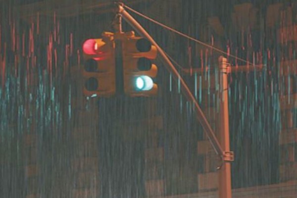
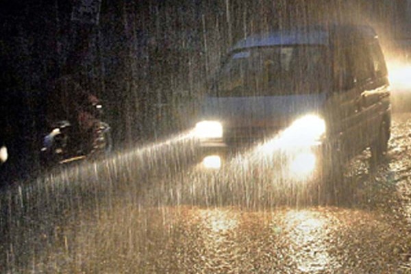
(a) Input

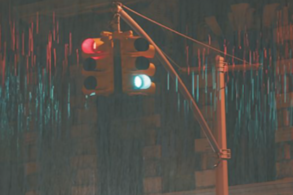
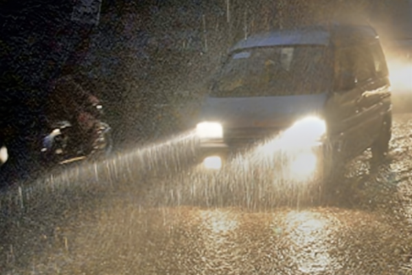
(b) Restormer [3]

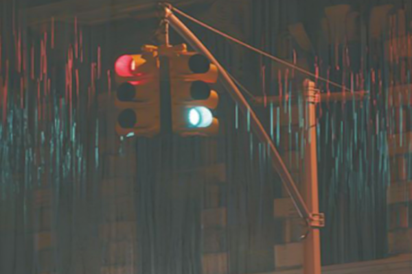
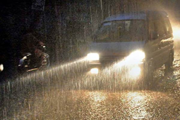
(c) M3SNet [4]

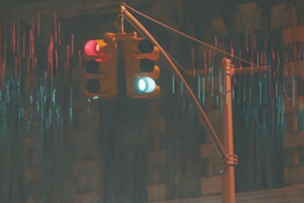
(d) SFNet [5]

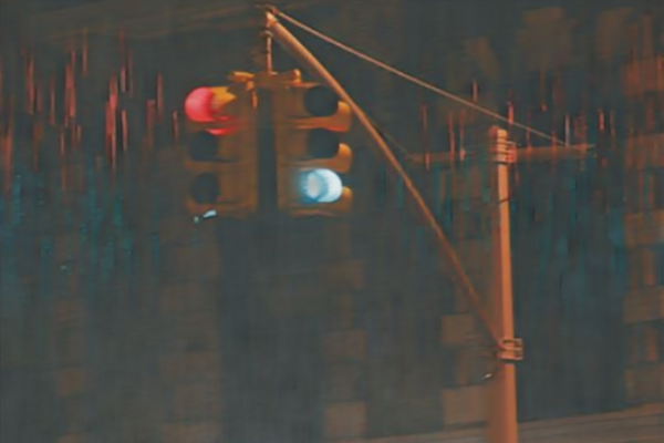
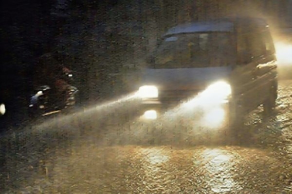
(e) PReNet [6]

Figure 1: Rain removal results of SOTA DL-based SIRR models on real nighttime rainy scene images. Images in the first row are rainy scene images input to SIRR models. From the second row to the fifth row, rain removal results of four SIRR models, Restormer [3], M3SNet [4], SFNet [5] and PReNet [6] are shown, respectively.

Data-driven SIRR approaches based on deep learning (DL) have gained a lot of traction due to their effective fitting capability [9]. The performance of DL-based methods is mainly affected by two key factors [9], i.e., the rationality and capacity of deraining models and the quality of training datasets. This paper mainly concentrates on the latter factor.

The current data acquisition methods for SIRR datasets can be broadly classified as real datasets, artificially generated datasets, and synthetic datasets. Real datasets [10, 11, 12] are acquired by capturing images of rainy scenes in the real world. However, this approach presents significant limitations as it depends on weather conditions and it is difficult to acquire paired rainy-clean images. On the other hand, artificially generated datasets [13] are created by simulating rainy scenarios in the real world, capturing clean background images, and pairing them with rainy images. However, this approach is time-consuming and labor-intensive. In contrast, image synthesis methods can synthesize rainy images from clean background images with little or no human intervention. These methods are faster and less labor-intensive, providing the potential to acquire large-scale paired rainy-clean image datasets. Therefore, existing SIRR models are typically trained on synthetic paired rainy-clean image datasets.

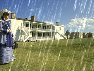
(a) Rain100L [14]

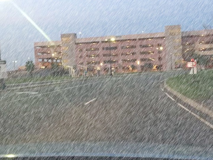
(b) BDD350 [15]

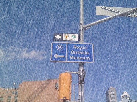
(c) COCO350 [15]

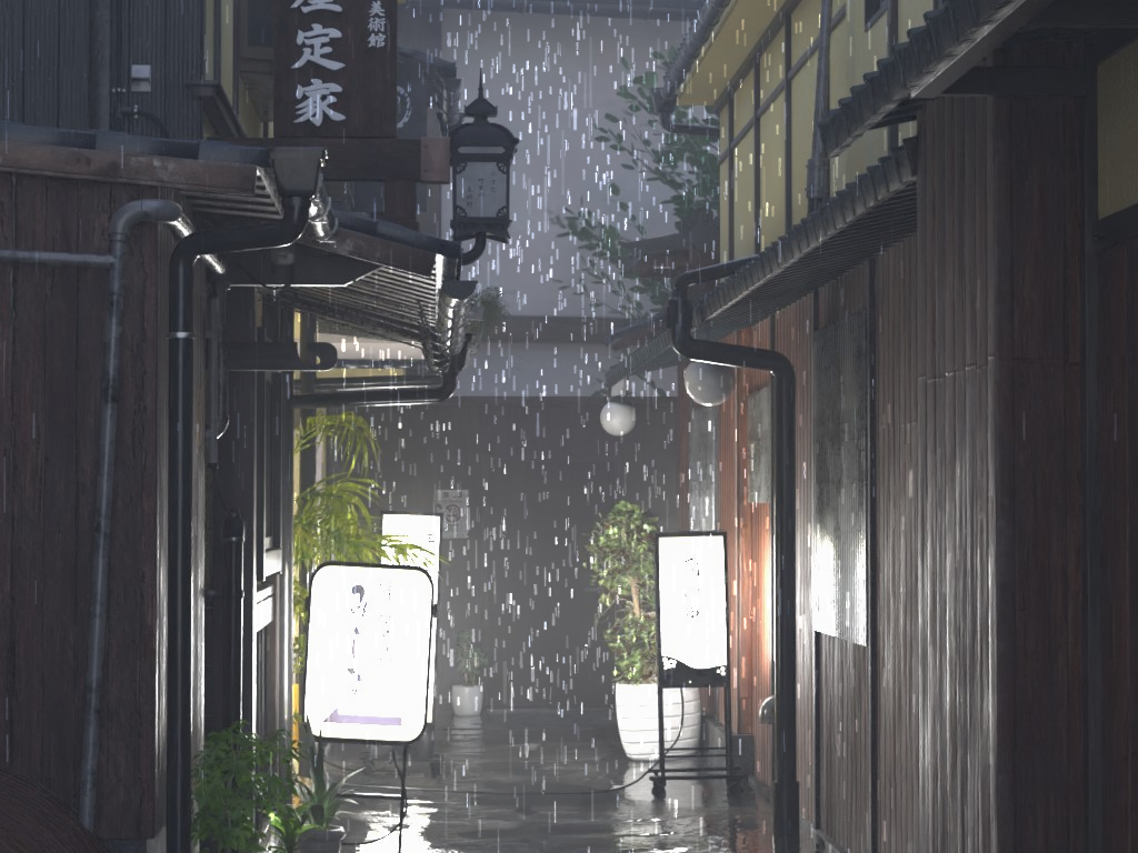
(d) HRI (Ours)

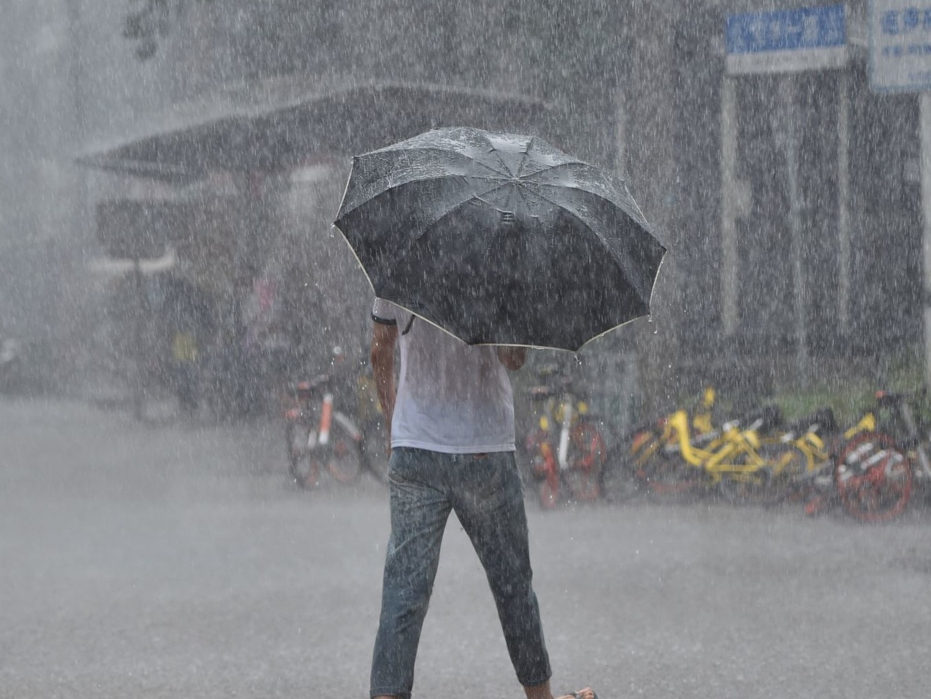
(e) Real Rain

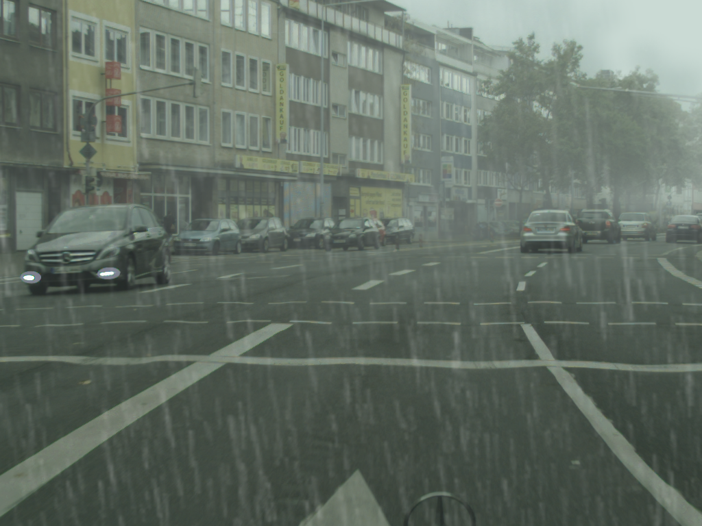
(f) RainCityscapes [16]

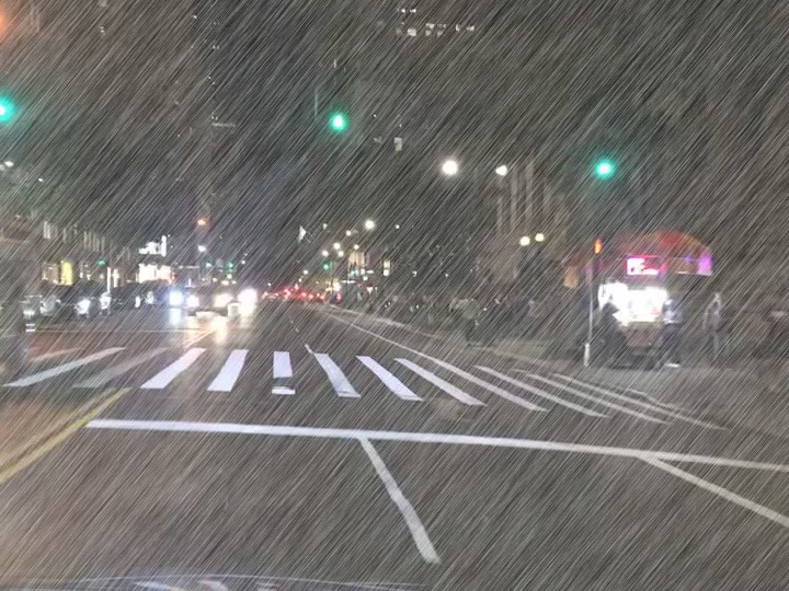
(g) BDD350 [15]

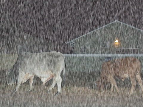
(h) COCO350 [15]

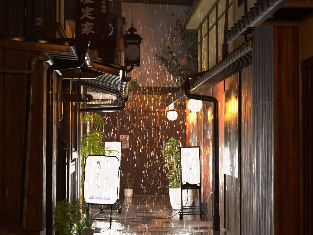
(i) HRI (Ours)

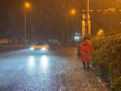
(j) Real Rain

Figure 2: Visual comparisons of real rainy images and synthetic rainy images from five datasets. Rain100L [14] and RainCityscapes [16] datasets only contain rainy images in daytime. BDD350 [15], COCO350 [15] and HRI (Ours) datasets contain rainy images in both daytime and nighttime. Real Rain is captured in real rain scenes.

Existing rainy image synthesis methods can be classified into two main categories, rendering-based methods and learning-based methods. Rendering-based methods [17, 1, 18, 19] focus on modeling the oscillation of raindrops and the appearance of rain streaks. These methods use a scene depth map, light source attributes, and specific custom rain attributes, to render realistic rain. Then, the rain layer is blended with the background image based on physical principles. On the other hand, learning-based methods [20, 9, 21, 22] aim to train generative models with real rainy image datasets to generate rainy images. In these methods, generative models can capture the complex distribution of rain patterns in real rainy images and efficiently generate diverse and non-repetitive rain patterns without human intervention and empirical parameters.

Despite the potential of these synthesis methods in generating synthetic rainy images, certain limitations persist. Rendering-based methods face challenges due to their complex input data and empirical parameters, which limits the diversity of synthetic rain. Physical simulation and rendering also significantly increase computational intensity and have substantial time overheads. Additionally, learning-based methods generate rain layers as grayscale and blend them with background images using linear overlaying. Moreover, these methods disregard optical phenomena like refraction and transmission, and ignore the color appearance of rain.

These issues have adversely affected the quality and diversity of training datasets, thereby limiting the performance improvement of SIRR models. We conduct an in-depth analysis of the currently available SOTA SIRR models, and observe that they perform well in daytime scenarios but poorly in complex illumination conditions such as at nighttime. As shown in Fig. 1, four DL-based SIRR models are presented for visual comparison of their deraining results on real nighttime rainy scene images. It can be clearly seen from these results that several SIRR models have struggled to completely remove colored rain streaks and restore a clean background. The PreNet [6] has the best rain removal results, able to remove the obvious white rain streaks (commonly appear in daytime rainy images), but it is difficult to remove rain streaks of other colors.

Through an analysis of existing synthetic rainy image datasets, we identify a lack of diversity in terms of illumination conditions, with a predominance of images captured during the daytime and a scarcity of images from complex illumination conditions such as at nighttime. Moreover, the resolution of synthetic images is generally low. These issues with image quality result in weak generalization ability of existing SIRR models in complex illumination conditions. Fig. 2 presents visual comparisons of real rainy images and synthetic rainy images randomly selected from five existing datasets: Rain100L [14], RainCityscapes [16], BDD350 [15], COCO350 [15] and HRI (Ours). Rain100L and RainCityscapes datasets only contain rainy images in daytime. BDD350, COCO350 and HRI datasets include rainy images in both daytime and nighttime. The rain layers in Rain100L, BDD350, and COCO datasets neglect the influence of scene illumination and depth, resulting in significant color appearance differences compared to real rainy images. Although RainCityscapes dataset takes scene depth into consideration, it does not include images under complex illumination conditions such as nighttime.

Consequently, there are few effective methods for synthesizing a mass of high-resolution rainy images in complex illumination conditions. However, these methods are essential for synthesizing large-scale high-quality (high resolution and complex illumination conditions) paired rainy-clean image datasets, which can train DL-based SIRR models capable of generalizing to various illumination conditions.

In this paper, to effectively synthesize a large quantity of high-resolution rainy images in complex illumination conditions, we propose a practical learning-from-rendering pipeline. The pipeline consists of two stages: the rendering stage, which creates high-resolution paired rainy-clean image datasets, and the learning stage, which trains a rainy image generation network using the datasets. The pipeline combines the benefits of the realism of rendering-based methods and the high-efficiency of learning-based methods, providing the possibility of creating large-scale high-quality paired rainy-clean image datasets.

To train a high-quality rainy image generation network, realistic paired rainy-clean image datasets are needed. Considering that collecting real rainy images captured by cameras is time-consuming, labor-cumbersome and difficult to obtain corresponding background images, we use a rendering-based method [1, 18, 19] to create a dataset in the rendering stage. Specifically, we create a High-resolution Rainy Image (HRI) dataset, which contains realistic high-resolution paired rainy-clean images of multiple scenes and various illumination conditions.

To learn illumination information from background images for high-resolution rainy image generation, we propose a High-resolution Rainy Image Generation Network (HRIGNet) in the learning stage. Considering that diffusion models [23, 24, 25] have been at the forefront of recent advances in image generative models, the HRIGNet is based on diffusion models.

Providing more useful guidance information for high-resolution image synthesis is expected to improve the quality of generated images. Inspired by ASSET [26], we design the HRIGNet to introduce a guiding diffusion model in the Latent Diffusion Model (LDM) [24]. To establish pairings between the generated rainy images and the input clean background images, it is necessary to apply effective constraints to the image synthesis process. Therefore, we use the cross-attention [27] and concatenation conditional mechanisms to control rainy image synthesis, using the latent code of the predicted rain layer image from the guiding diffusion model and the masked background image as conditioning respectively.

In summary, our work makes the following contributions:

• We propose a practical two-stage learning-from-rendering pipeline for high-resolution rainy image synthesis, which combines the benefits of the realism of rendering-based methods and the high-efficiency of learning-based methods, providing the possibility of creating large-scale high-quality (high resolution and complex illumination conditions) paired rainy-clean image datasets.

• In the rendering stage, we use a rendering-based method to render realistic rainy images and create a HRI dataset for the training of the rainy image generation network in the learning stage. The HRI dataset contains realistic high-resolution paired rainy-clean images of multiple scenes and various illumination conditions.

• In the learning stage, we propose a diffusion-based method HRIGNet, which can learn illumination information from background images for high-resolution rainy image generation, taking advantage of the high-efficiency of the learning-based method. Rain removal experiments on real dataset validate that our HRIGNet can help improve the robustness of deep derainers to rainy images in the real world.

The remainder of this paper is organized as follows. Sect. II introduces the related work. Our proposed learning-from-rendering pipeline is presented in Sect. III. Our proposed HRIGNet is presented in Sect. IV. Experimental results are reported in Sect. V. Finally, Sect. VI concludes the paper.

II Related Work

TABLE I: Shortcomings or irrationalities of existing rain datasets or acquisition methods.

name	type	key idea	shortcomings or irrationalities
MPID [10]	real rain	Images of real-world rainy scenes captured by cameras are collected from the Internet.	1. Clean background images are not included. 2. Time-consuming and labor-cumbersome.
RainDS [13]	artificially generated rain	They sprayed water using sprinklers to mimic rainy scenes in the real world and obtained paired rainy-clean images.	1. The types of artificially simulated rain scenes are limited, and there are certain differences with the real rain scenes. 2. Time-consuming and labor-cumbersome.
SPA-Data [28]	artificially synthetic rain	A semi-automatic method that incorporates temporal properties of rain streaks and human supervision to generate clean images from sequences of real rain images.	Human supervision is needed.
MPID [10]	artificially synthetic rain	Rainy images are synthesized from clean images through Photoshop.	Scene depth is lack of consideration.
Photorealistic rendering [17]	rendering-based synthesis	They developed a model for rain streak appearance and an image-based rendering algorithm for realistic rain rendering.	1. Complex input data and empirical parameters limits the diversity of synthetic rain. 2. Physical simulation and rendering increase substantial time overheads.
Physics-based rendering [1]	rendering-based synthesis	They proposed a practical, physically-based approach to render realistic rain in images.	Physical simulation and rendering increase substantial time overheads.
RainCityscapes [16]	rendering-based synthesis	It was created by adopting the images in the Cityscapes dataset as clean background images, leveraging the rain streak appearance model.	Physical simulation and rendering increase substantial time overheads.
RICNet [20]	learning-based synthesis	They propose a GAN-based rain intensity controlling network to control the rain continuously in a bi-directional manner.	Some essential attributes of rain are disregard, including color and optical phenomena.
JRGR [22]	learning-based synthesis	They proposed a CycleGAN-based unified framework that jointly learns rain generation and removal.	Some essential attributes of rain are disregard, including color and optical phenomena.
VRGNet [9]	learning-based synthesis	They proposed a VAE-based generative model to depict the generation process of rainy images, which can explore an implicit distribution of the rain in statistics.	Some essential attributes of rain are disregard, including color and optical phenomena.

II-A Rain Dataset Acquisition

As mentioned above, the data acquisition methods for SIRR datasets can be broadly classified as real datasets, artificially generated datasets, and synthetic datasets. In this subsection, they will be reviewed and analyzed deeply.

Li et al. [10] proposed a large-scale image deraining benchmark dataset, which includes three sets of real-world rainy images. They were obtained by collecting images of real-world rainy scenes captured by cameras from the Internet, but they do not include paired clean background images. Quan et al. [13] sprayed water using sprinklers to generate rain streaks and mimic rainy scenes in the real world. By stopping spraying water, they obtained the clean background images. Although this method can obtain clean and rainy scene image pairs, it is time-consuming and labor-cumbersome.

Wang et al. [28] proposed a semi-automatic method that incorporates temporal properties of rain streaks and human supervision to generate high quality clean images from sequences of real rainy images. Due to the need for human supervision, this method is also time-consuming and labor-cumbersome. Li et al. [10] synthesized rainy images from clean images of outdoor cloudy and fog-free scenes through Photoshop. However, the lack of consideration for scene depth in this method significantly deviates from the characteristics exhibited in real rainy images.

Garg and Nayar [17] studied the visual appearance of rain streaks in detail for the first time. They developed a model for rain streak appearance and an image-based rendering algorithm for realistic rain rendering under different illumination. Based on their work, Halder et al. [1] proposed a practical, physically-based approach to render realistic rain in images. The RainCityscapes [16] dataset was also created by adopting the images in the Cityscapes [29] dataset as clean background images, leveraging the rain streak appearance model. Despite these rendering-based methods capable of rendering realistic rain under specific illumination, they come with their limitations. Users are required to specify the rain parameters, and the raindrop distribution is simulated based on physical methods, which makes capturing the complex raindrop distribution in real rainy images challenging.

To efficiently generate diverse and non-repetitive rain streaks, some researchers have utilized deep learning for rainy image synthesis. Ni et al. [20] propose a GAN-based [30] rain intensity controlling network to control the rain continuously in a bi-directional manner while preserving the scene-specific rain characteristics. Ye et al. [22] proposed a CycleGAN-based [31] unified framework that jointly learns rain generation and removal, offering a better approximation to real rain by learning physical degradation from real rainy images. Wang et al. [9] proposed a VAE-based [32] generative model to depict the generation process of rainy images, which can explore an implicit distribution of the rain layers in statistics, so they obtained an interpretable rain generator.

Although these DL-based methods can efficiently synthesize rainy images, they still have some limitations. Typically, these methods treat the rain layer as a gray-scale layer and blend it with the background image using linear overlaying. Consequently, they disregard other essential attributes of rain, including color and optical phenomena like refraction and transmission. Besides, existing synthetic rainy image datasets lack diversity in terms of illumination conditions, with images mainly in daytime illumination conditions, and few images in complex illumination conditions, like nighttime. Further, the resolution of these synthetic rainy images is typically low. In this paper, we propose a practical learning-from-rendering pipeline, which combines the realism advantages of rendering-based methods and the high-efficiency advantages of learning-based methods, providing the possibility of creating large-scale high-quality paired rainy-clean image datasets.

Shortcomings or irrationalities of existing rain datasets or acquisition methods are summarized in Table I.

II-B Generative Models for Image Synthesis

As mentioned above, GANs and VAEs, as DL-based generative models, have been utilized in rainy image synthesis. Nevertheless, these generative models possess certain limitations. GANs [30] produce high-quality images through adversarial training, but their optimization is challenging. In contrast, VAEs [32] rely on likelihood estimation, allowing for faster generation of high-quality images, but the image quality may not be as good as that of GANs. Diffusion models [23, 24, 25] have achieved state-of-the-art results in the field of image synthesis. However, the original diffusion models [23] are slow in sampling, as they need a mass of time steps to generate a sample. Consequently, Latent Diffusion Models (LDMs) [24] use a two-stage pipeline, firstly compressing images into a low-dimensional latent space, and training diffusion models on the compressed latent space, which speeds up the training and inference process with almost no reduction in synthesis quality. Given its high-quality image generation capability, our proposed rainy image generation network is based on LDM.

II-C Conditional Image Synthesis

Conditional image synthesis allows users to control the image synthesis process, allowing for applications such as semantic image editing, image inpainting, etc. Conditional diffusion models [33, 24] are capable of modeling conditional distributions of the form $p(z|y)$, which enables controlling the synthesis process through inputs $y$ such as text, semantic map, etc.

High-resolution images synthesis is a challenging task, having high demand in terms of quality and computational complexity. Providing more useful guidance information [26, 34, 35], such as low-resolution images and intermediate generation results, is expected to improve the quality of generated images.

Inspired by ASSET [26], our proposed HRIGNet is designed to introduce a guiding diffusion model in the LDM [24]. Given a clean background image and a mask of a rain layer, the HRIGNet generates the latent code of the rain layer image with a guiding diffusion model. The latent code is then used to guide the diffusion process for high-resolution image synthesis.

III Learning From Rendering

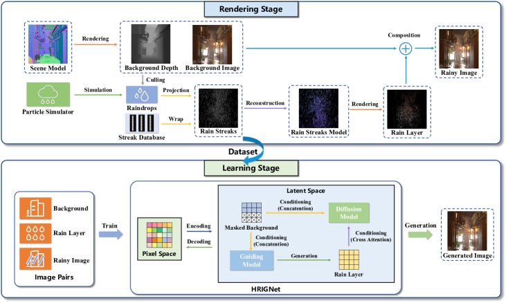
Figure 3: Overview of our learning-from-rendering pipeline for high-resolution rainy image synthesis. The top is the rendering stage, the bottom is the learning stage, and the two stages are interlinked via rainy image datasets.

In rainy weather, images captured by cameras are usually disturbed by rain in the scene and suffer from degradation such as rain streaks, raindrops, fog-like rain, etc. In this paper, we mainly focus on the phenomenon of rain streaks, which occurs when falling raindrops produce motion-blurred streaks during the exposure time of the camera. Rainy images mentioned in this paper refer to images that have been degraded by rain streaks.

To effectively synthesize a large quantity of high-resolution rainy images in complex illumination conditions, we propose a practical two-stage learning-from-rendering pipeline, as shown in Fig. 3. Specifically, the pipeline combines rendering-based and learning-based methods, and consists of two stages: the rendering stage and the learning stage. In the rendering stage, we use a rendering-based method to render realistic high-resolution paired rainy-clean images and create paired rainy-clean image datasets. In the learning stage, we train a rainy image generation network using the rendered datasets to efficiently generate high-resolution rainy images. The pipeline combines the benefits of the realism of rendering-based methods and the high-efficiency of learning-based methods, providing the possibility of creating large-scale high-quality paired rainy-clean image datasets.

III-A Rendering Stage

To train a high-quality rainy image generation network, we need realistic paired rainy-clean image datasets under various illumination conditions. Considering that collecting real rainy images captured by cameras is time-consuming, labor-cumbersome, and difficult to obtain corresponding background images, we use a rendering-based method.

Offline rendering techniques based on ray tracing algorithm [18] can simulate most natural phenomena of object surface interactions in the real world and produce realistic images. Currently, these techniques have found extensive use in the fields of movies, animation, and design. Blender [19] is a popular free and open-source 3D creation suite utilized to create 3D scene models with ease, supporting various common light sources. Cycles, Blender’s powerful built-in unbiased path-tracer engine can render realistic rainy images.

We use Blender and the image-based rain rendering algorithm [17, 1] in the rendering stage. The rendering pipeline is shown in Fig. 3. Specifically, we use modeling tools to create 3D scene models and render them with Cycles engine to obtain background scene RGB images and depth images. Based on our raindrop physical particle simulator, we generate raindrop particles in the scene, excluding invisible ones to reduce the amount of rendering data. With the rain streak rendering algorithm of Garg and Nayar [17], we sample rain streaks from the rain streak database and project them in the image. Then each rain streak pixel is reconstructed into a quad to obtain the rain streaks 3D models. After merging the rain streaks 3D models with the background scene 3D model, we render the result rainy scene 3D model to obtain illuminated rain layers. Finally, we blend rain layers with background images to obtain synthetic rainy images. Each image pair therefore includes a background image, a depth image, a rain layer image, and a rainy image.

Background rendering. With the Cycles engine, the pre-created scene 3D model is rendered to obtain realistic background RGB images and depth images. To capture the scene under different illumination conditions in a full day, we use procedural sky in the scene and set equal time intervals between 0 and 24 hours. For the camera parameter settings, we used focal lengths between 30mm and 50mm, and a shutter speed of 1/60s [17] (for motion blur effects in dynamic scenes).

Raindrops generation. To accurately align with the size and distribution of raindrops in the real world, we implement a raindrop particle physics simulator with reference to existing theoretical studies of raindrop dynamics [36, 37, 38, 39]. The simulation involves the size distribution, terminal velocity, and spatial distribution of raindrops.

Rain attributes, including the intensity and direction of rain, can be controlled as input parameters in our simulator. The intensity of rain is the volume of water delivered to the ground per unit of ground surface and per unit of time [36]. Rain can be classified into light rain, moderate rain and heavy rain [37, 36] according to the intensity. Our HRI dataset (presented in Sect. III-B) includes different intensities of rain ranging from 5 to 200 mm/h, covering common intensities. The rain size distribution (RSD) and the terminal velocity of raindrops is rather dependent on the intensity of rain. The exponential RSD of Marshall and Palmer [38] and the terminal velocity of Kessler [39] are used here. For simplicity, we use a random uniform distribution to simulate the initial spatial distribution of raindrops and add additional velocity to the raindrops based on the input wind size and direction.

More information about our raindrop particle physics simulator can be found in Appendix A.

Rain streaks generation. Considering that the raindrops generated by our simulator are not fully visible to the camera, we cull the invisible raindrops to reduce the amount of rendering data. Based on the camera parameters, we first cull the raindrops outside the frustum. Then, based on the scene depth map and the position of the raindrops, we further cull the raindrops that are occluded by the scene. We sample rain streaks from the rain streak database [17] and project them in the image according to the image-based rain rendering algorithm [1].

Rain streaks rendering. In the image-based rain rendering algorithm [17], raindrops are needed to be illuminated with the light sources in the scene. To give the raindrops consistent illumination with the background scene, we create a quad at the position of each raindrop pixel in the scene, producing the rain streaks 3D models. After combining the rain streaks 3D models with the scene 3D model, we render them with the same illumination conditions as the background scene to obtain a illuminated rain layer.

Rainy image composition. After obtaining the background images and illuminated rain layer images, we composite them to obtain rainy images. According to the image-based rain rendering algorithm [1], suppose $\mathbf{x}$ a pixel in the background image $I$ and $\mathbf{x}^{\prime}$ the overlapping coordinates in rain layer $S^{\prime}$, the result of the blending is obtained with:

$$I_{rainy}(\mathbf{x})=\frac{T-S^{\prime}_{\alpha}(\mathbf{x^{\prime}})\tau_{1}}{T}I(\mathbf{x})+S^{\prime}(\mathbf{x^{\prime}})\frac{\tau_{1}}{\tau_{0}},$$ (1)

where $S^{\prime}_{\alpha}(\mathbf{x^{\prime}})$ is the alpha channel of the rain layer, $T$ is the targeted exposure time, $\tau_{0}=\sqrt{10^{-3}}/50$ is the time for which the raindrop remained on one pixel in the streak database, and $\tau_{1}$ the same measure according to our physical simulator.

III-B High-resolution Rainy Image Dataset

In the rendering stage, we create a High-resolution Rainy Image (HRI) dataset. The HRI dataset comprises a total of 3,200 image pairs. Each image pair comprises a clean background image, a depth image, a rain layer mask image, and a rainy image. As shown in Table II, it contains three scenes: lane, citystreet and japanesestreet, with image resolutions of $2048\times 1024$. The lane scene contains 1,600 image pairs, consisting of images from 4 camera viewpoints, with each viewpoint containing 100 images of different moments, and each moment containing 4 different intensities of rainy scenes. The citystreet scene contains 600 image pairs, consisting of images from 6 camera viewpoints, with each viewpoint containing 25 images of different moments, and each moment containing 4 different intensities of rainy scenes. The japanesestreet scene contains 1,000 image pairs, consisting of images from 10 camera viewpoints, with each viewpoint containing 25 images of different moments, and each moment containing 4 different intensities of rainy scenes. Some rainy images of the HRI dataset are shown in Fig. 4.

We split the HRI dataset into training set and test set according to camera viewpoints. For the lane scene, the training set contains images from 3 camera viewpoints, and the test set contains images from 1 camera viewpoint. For the citystreet scene, the training set contains images from 5 camera viewpoints, and the test set contains images from 1 camera viewpoint. For the japanesestreet scene, the training set contains images from 8 camera viewpoints, and the test set contains images from 2 camera viewpoints. Therefore, the training set comprises a total of 2,500 image pairs, and the test set comprises a total of 700 image pairs.

TABLE II: Overview of the HRI dataset.

scene	dataset type	resolution	viewpoints	moments	intensities	image pairs
lane	training set	$2048\times 1024$	3	100	4	1,200
	test set		1			400
citystreet	training set	$2048\times 1024$	5	25	4	500
	test set		1			100
japanesestreet	training set	$2048\times 1024$	8	25	4	800
	test set		2			200

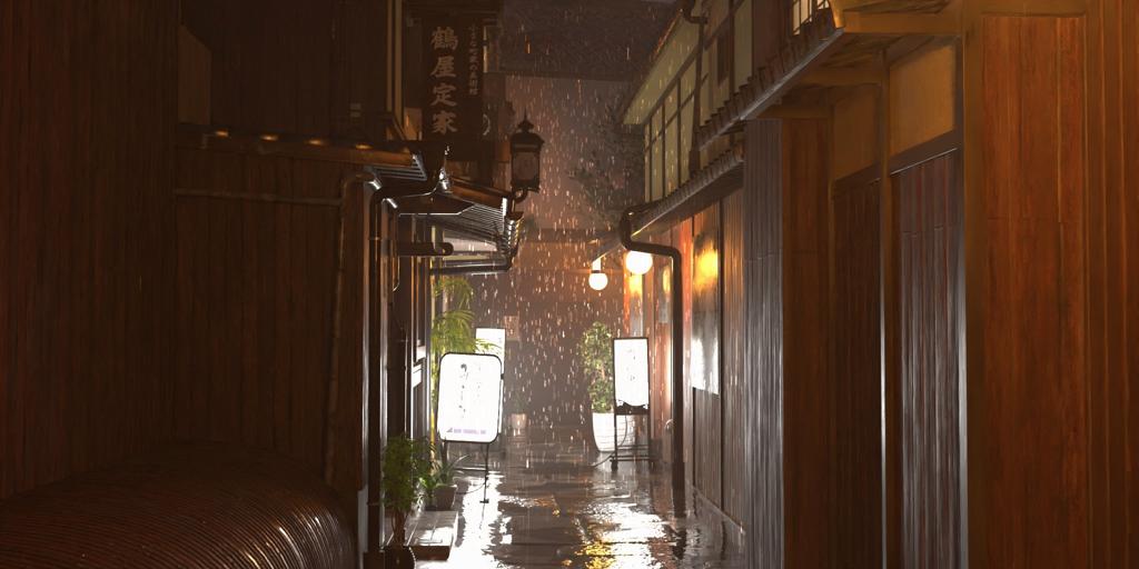
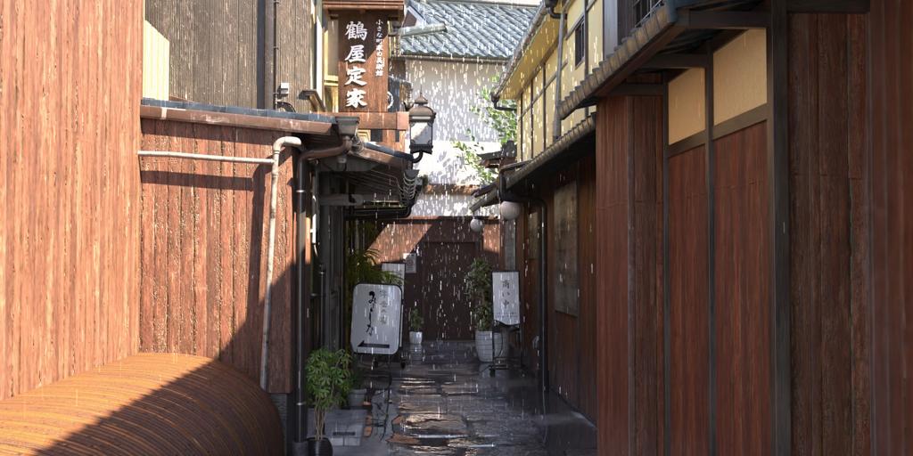
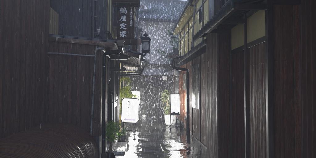
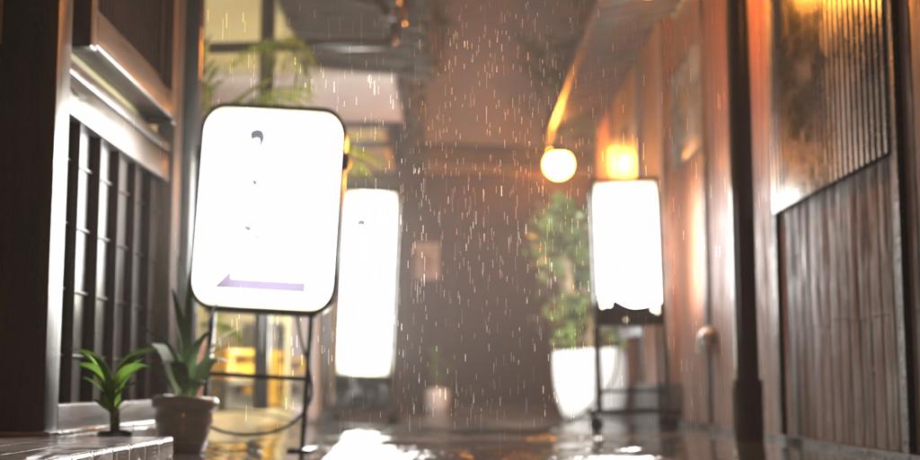
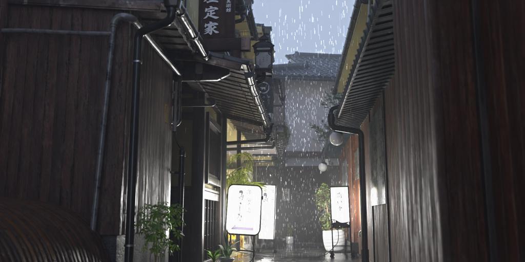
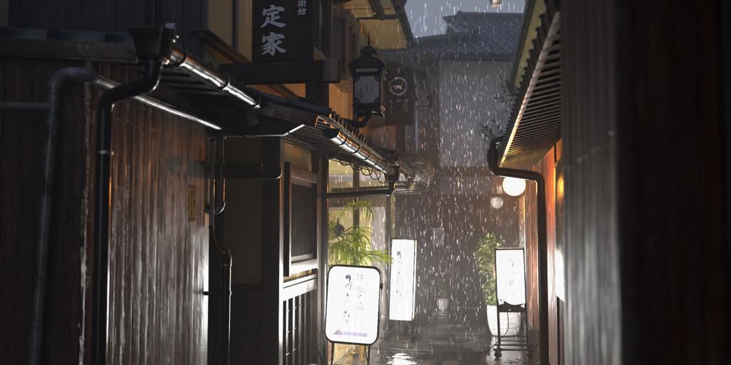
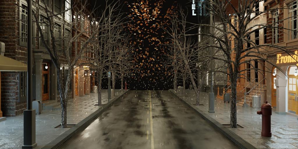
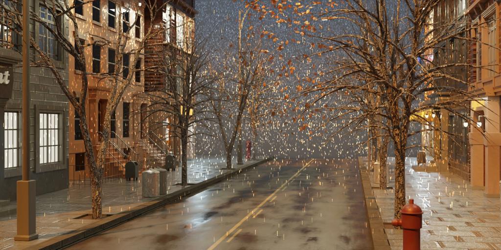
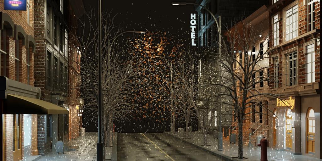
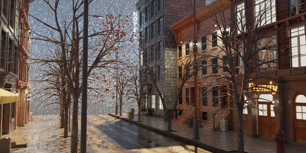
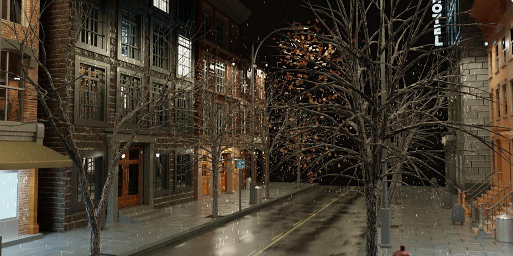
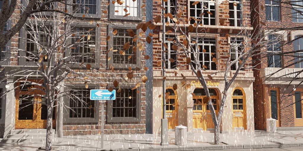
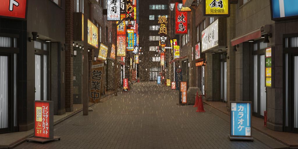
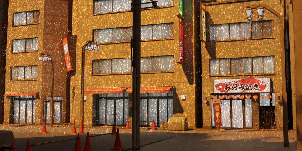
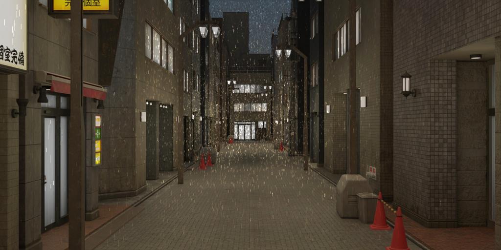
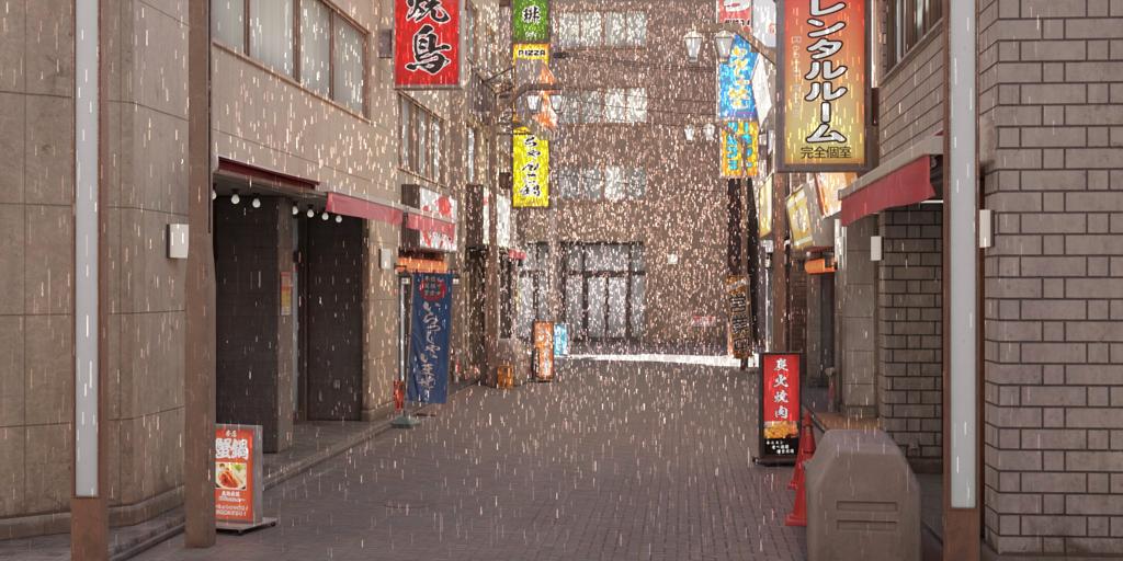
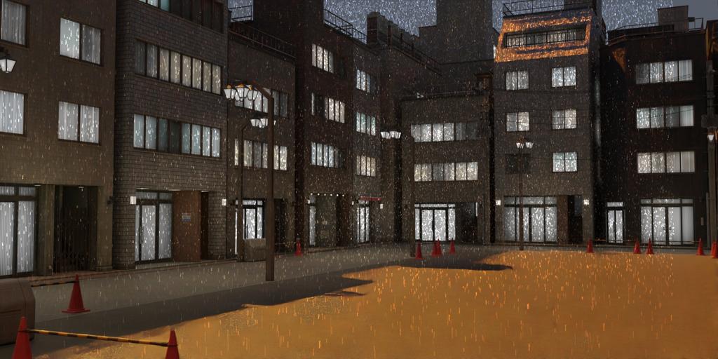
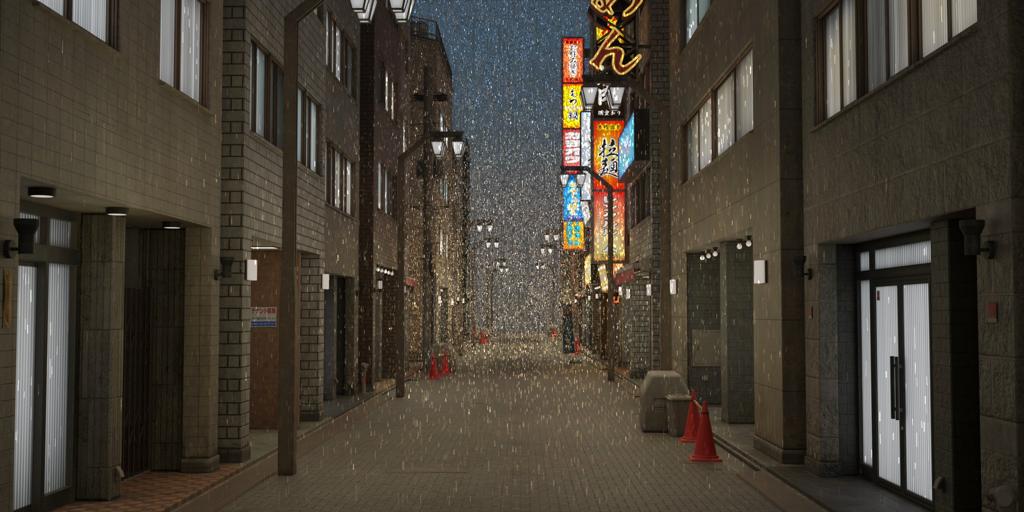
Figure 4: Rainy images of the HRI dataset. The first row is the rainy images of the lane scene. The second row is the rainy images of the citystreet scene. The third row is the rainy images of the japanesestreet scene.

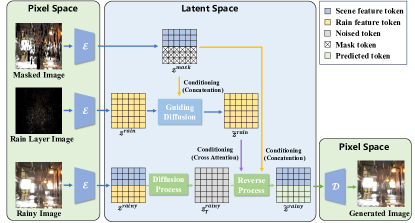
Figure 5: The overall architecture of HRIGNet. We use a guiding diffusion model to predict the latent code of rain layer images, and then use them together with the latent code of masked background images as conditioning to guide the synthesis of high-resolution rainy images.

IV High-resolution Rainy Image Generation Network

In the learning stage, we propose a High-resolution Rainy Image Generation Network (HRIGNet), which synthesizes high-resolution rainy images from clean background images and corresponding rain layer masks. More specifically, given a RGB background image and a mask indicating the positions of rain streaks in the scene, HRIGNet can generate rain streaks at the corresponding positions, with illumination conditions and color appearance consistent with the background image. In addition, our method is capable of generating high-resolution images up to $2048\times 1024$ resolution.

The architecture of HRIGNet is shown in Fig. 5. According to the LDM [24], to reduce the computational cost of training diffusion models on high-resolution images, an autoencoding model [40] is used to learn a latent space that is perceptually equivalent to the image space. The encoder can compress images perceptually to obtain latent code in the latent space that is equivalent to pixels in the image space. So the forward and reverse processes of diffusion models can be conducted in the latent space. Finally, the output latent code is decoded back into the image space by the decoder.

To control the image synthesis process of diffusion models, we use concatenation and cross-attention as two conditional mechanisms to control the reverse process. Inspired by ASSET [26], we first use a guiding diffusion model to predict the latent code of rain layer images, and then use the latent code to enhance the underlying UNet backbone [41] of diffusion models via the cross-attention conditioning mechanism. The predicted rain layer images can provide more guidance information to improve the quality of generated rainy images. To impose stronger constraints on the image synthesis process, we composite the background image and rain layer mask as a masked image, and use it as conditioning for the reverse process via the concatenation conditioning mechanism.

IV-A Latent Diffusion Models

Diffusion models[23, 24, 25] are probabilistic models that gradually add noise to the data by traversing a Markov chain of $T$ time steps, transforming the distribution of real data to a Gaussian distribution. The forward process of diffusion models adds noise step by step to the real data $x_{0}\sim q(x_{0})$, with $q(x_{t}|x_{0})=\mathcal{N}(x_{t};\sqrt{\bar{\alpha}_{t}}x_{0},(1-\bar{\alpha}_{t})\mathbf{I})$, where $\bar{\alpha}$ is a hyperparameter, and $x_{1},\dots,x_{T}$ are latent codes with the same dimensions as the real data $x_{0}$. By applying the reparameterization trick [23], we can sample $x_{t}=\sqrt{\bar{\alpha}_{t}}x_{0}+\sqrt{1-\bar{\alpha}_{t}}\epsilon_{t}$ at any time step, where $\epsilon_{t}\sim\mathcal{N}(0,\mathbf{I})$. Diffusion models are trained to learn the reverse process, which is the inverse transformation of the forward process, gradually removing noise from the variable $x_{t}\sim\mathcal{N}(0,\mathbf{I})$ by applying a learnable Gaussian transformation $p_{\theta}(x_{t-1}|x_{t})=\mathcal{N}(x_{t-1};\mu_{\theta}(x_{t}),\Sigma_{\theta}(x_{t}))$, where neural networks are used to predict the statistics $\mu_{\theta}$ and $\Sigma_{\theta}$ of $p_{\theta}$. $\mu_{\theta}$ is then reparameterized as a denoising network $\epsilon_{\theta}(x_{t},t)$, and the corresponding objective can be simplified as

$$L_{DM}=\mathbb{E}_{x,\epsilon\sim\mathcal{N}(0,1),t}\Big{[}\left\|\epsilon-\epsilon_{\theta}(x_{t},t)\right\|_{2}^{2}\Big{]},$$ (2)

where $t$ is uniformly sampled from $\{1,\dots,T\}$.

In order to reduce the computational cost of training diffusion models on high-resolution images, LDM [24] first trains a perceptual compression autoencoding model VQGAN [42]. VQGAN consists of an encoder $\mathcal{E}$ and a decoder $\mathcal{D}$. The encoder compresses images from the high-dimensional image space to a low-dimensional latent space, where high-frequency and imperceptible details are abstracted away. This makes training of diffusion models more efficient in the low-dimensional latent space. Given a high-resolution RGB rainy image $x^{rainy}$, the corresponding latent code encoded by the encoder is $z^{rainy}$. So the objective of LDM can be expressed as

$$L_{LDM}=\mathbb{E}_{\mathcal{E}(x^{rainy}),\epsilon\sim\mathcal{N}(0,1),t}\Big{[}\left\|\epsilon-\epsilon_{\theta}(z_{t}^{rainy},t)\right\|_{2}^{2}\Big{]}.$$ (3)

Here, the neural backbone $\epsilon_{\theta}(\circ,t)$ of LDM is realized as a UNet [41].

IV-B Guiding Diffusion Model

Using the intermediate generation results as guidance can provide more information for high-resolution image synthesis, which is expected to improve the quality of generated images. Therefore, we use a guiding diffusion model (GDM) trained on the latent codes of rain layer images. Since the latent codes have a lower dimensionality, the GDM can efficiently perform the training and sampling process. The GDM coarsely predicts the latent codes of the rain layer images, which are used as conditioning in the reverse process of the diffusion model to guide high-resolution image synthesis.

Specifically, we first composite the input RGB background image and rain layer mask to obtain the masked image $x^{mask}$. Then the masked image is encoded into the latent space to obtain the latent codes $z^{mask}$, which are input to the GDM to predict the latent code of rain layer image $\tilde{z}^{rain}$. The objective of GDM can be expressed as

$$L_{GDM}=\mathbb{E}_{\mathcal{E}(x^{rain}),\epsilon\sim\mathcal{N}(0,1),t}\Big{[}\left\|\epsilon-\epsilon_{\theta}(z_{t}^{rain},t,z^{mask})\right\|_{2}^{2}\Big{]}.$$ (4)

Here, the neural backbone of GDM is also realized as a UNet [41].

IV-C Conditioning Mechanisms

By modeling the reverse process of diffusion models as conditional distributions $p(z|y)$, constraints can be imposed on the reverse process to control the image synthesis. This can be implemented with a conditional denoising network $\epsilon_{\theta}(z_{t},t,y)$. In the context of image synthesis, LDMs use the cross-attention mechanism [27] to enable inputs from different modalities to serve as conditionings for DMs. Our method leverages the predicted latent code of the rain layer image by GDM as conditioning via the cross-attention mechanism. Specifically, $\tilde{z}^{rain}$ is mapped to the intermediate layers of the UNet via a cross-attention layer represented as Attention$(Q,K,V)=$softmax$(\frac{QK^{T}}{\sqrt{d}})\cdot V$, where

$$Q=W^{(i)}_{Q}\cdot\varphi_{i}(z_{t}^{rainy}),K=W^{(i)}_{K}\cdot\tilde{z}^{rain},V=W^{(i)}_{V}\cdot\tilde{z}^{rain}.$$

Here, $\varphi_{i}(z_{t}^{rainy})$ represents the intermediate representation of $\epsilon_{\theta}$ implemented by UNet, and $W^{(i)}_{Q},W^{(i)}_{K},W^{(i)}_{V}$ are learnable projection matrices.

Moreover, to enhance the constraints on the image synthesis process, we utilize the concatenation conditioning mechanism, in conjunction with the cross-attention conditioning mechanism. We use the latent code of masked image $z^{mask}$ as conditioning of the reverse process via the concatenation conditioning mechanism. Specifically, the input of the reverse process are $z_{t}^{concat}=[z^{rainy}_{t},z^{mask}]$.

Via the concatenation and cross-attention conditioning mechanisms, we then learn the conditional LDM via

$$L_{LDM}=\mathbb{E}_{\mathcal{E}(x^{rainy}),\epsilon\sim\mathcal{N}(0,1),t}[\left\|\epsilon-\epsilon_{\theta}(z_{t}^{concat},t,\tilde{z}^{rain})\right\|_{2}^{2}].$$ (5)

Combining the two objective functions in Eq. 4 and Eq. 5, the total objective of HRIGNet is

$$L_{HRIG}=L_{GDM}+L_{LDM}$$ (6)

IV-D Image Generation

Our proposed HRIGNet is based on LDM, where the encoder of VQGAN compresses the original image into a low-dimensional latent space. For images of size $H\times W$ and a number of downsampling blocks of $m$, the input latent code to the diffusion model is of size $H/2^{m}\times W/2^{m}$, which reduces the spatial cost of training and speeds up the training and inference processes. However, when $m$ exceeds a critical value, the reconstruction quality degrades [42]. Therefore, during training, we have to work patch-wise and crop images. Specifically, we train our model using images of up to $512\times 512$ resolution. During inference, to generate higher-resolution images, considering that spatial conditioning information [42] is available in our model, we can simply segment background images into patches of size $512\times 512$ and use them as conditioning. By merging the output results, we can generate images with resolutions higher than $512\times 512$. In our experiments, our model can generate images up to $2048\times 1024$ resolution.

In our implementation, we find that if background images is simply segmented into blocks and input them into the model, the output results will have slight variations in hue, which will cause the merged output to produce a block effect. To fix this issue, we use the rain layer masks to blend the generated images with the background images.

V Experimental Results

In this section, we compare our proposed HRIGNet with some commonly used baseline image generative models to evaluate its performance in high-resolution rainy image synthesis, and conduct an ablation study to evaluate the effect of using guiding models with different guiding information and resolutions. To further validate that our HRIGNet can help improve the robustness of deep derainers to rainy images in the real world, we retrain the derainers on datasets augmented by the HRIGNet and evaluate their deraining performance.

V-A Implementation Details

To train our HRIGNet, we first use rain layer images with a size of $512\times 512$ to pretrain a GDM based on the loss function in Eq. 4. Then with the parameters of the GDM fixed, the HRIGNet is trained using rainy images with a size of $512\times 512$ based on the loss function in Eq. 5.

We adopt AdamW [43, 44] optimizer in the training process of both the GDM and the HRIGNet. The first stage model and the conditioning stage model share a same VQGAN model, with the parameters of the model using pretrained vq-f4 from LDM. The initial learning rate of the diffusion model is set as $2\times 10^{-6}$, the batch size is 1, the image size of the UNet backbone is $128\times 128$, and the model channels are 224.

The experiments are implemented on PyTorch [45] platform with an NVIDIA GeForce RTX 3090 GPU.

V-B Compare With Baselines

(a) Background

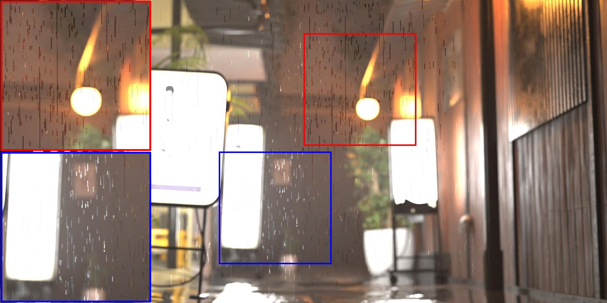
(b) LDM [24]

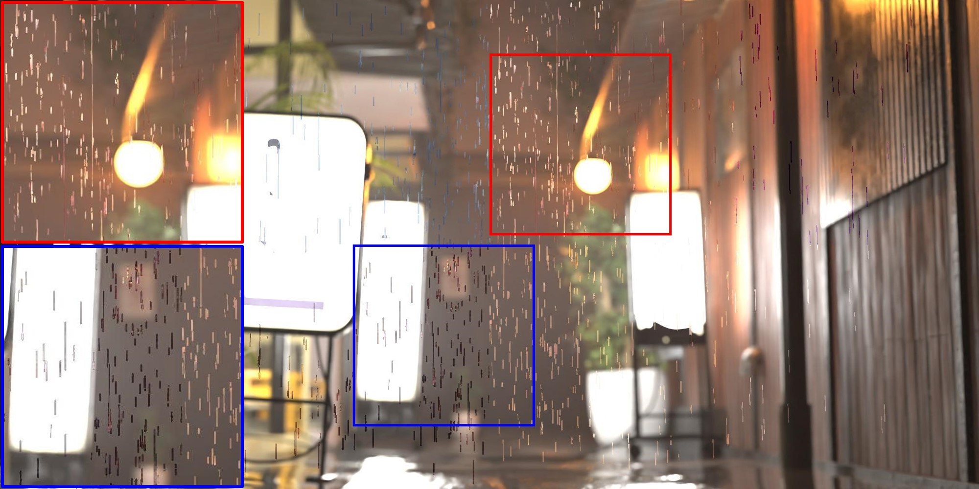
(c) DiT [25]

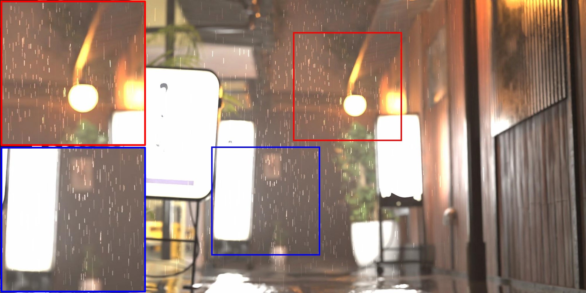
(d) Ground truth

(e) CycleGAN [31]

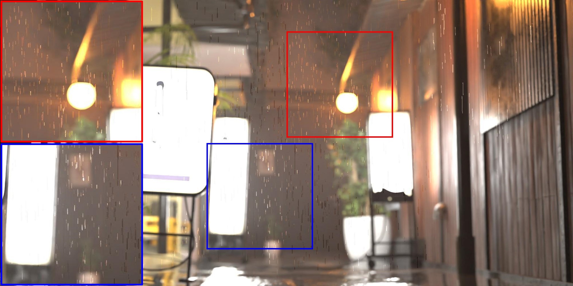
(f) HRIGNet (ours)

Figure 6: Visual comparison of generated rainy images from different image generative models. Our HRIGNet can better capture the illumination and color in the background image, and map them to the generated rain layer.

TABLE III: Quantitative evaluation of baseline models and HRIGNet.

method	patch size	FID$\downarrow$	LPIPS$\downarrow$	SSIM$\uparrow$	PSNR$\uparrow$
LDM [24]	512$\times$512	46.583	0.241	0.703	16.652
DiT [25]	512$\times$512	164.977	0.490	0.548	12.097
CycleGAN [31]	512$\times$512	47.073	0.271	0.639	21.604
HRIGNet	512$\times$512	32.111	0.205	0.747	18.595

In order to evaluate the performance of HRIGNet in high-resolution rainy image synthesis, we compare it with several baseline image generative models: LDM [24], DiT [25] and CycleGAN [31]. The evaluation metrics used are FID [46], LPIPS [47], SSIM [48], and PSNR [49]. More information about the model settings can be found in Appendix B-A. As the results shown in Table III, our model achieves state-of-the-art results in FID, LPIPS and SSIM. Fig. 6 illustrates a comparison of rainy image synthesis results of these methods. As seen, our method can well capture the illumination and color in the background image, and map them to the generated rain layer. As a result, the rain layer is endowed with a visually plausible color appearance that matches the background image.

TABLE IV: Quantitative evaluation of guiding models.

guiding information	resolution	FID$\downarrow$	LPIPS$\downarrow$	SSIM$\uparrow$	PSNR$\uparrow$
Rainy Image	256$\times$256	150.851	0.505	0.389	13.692
Rain Layer	256$\times$256	149.779	0.506	0.390	13.674
Rain Layer	512$\times$512	32.111	0.205	0.747	18.595

TABLE V: Quantitative evaluation of HRIGNet with different backbones.

backbone	resolution	FID$\downarrow$	LPIPS$\downarrow$	SSIM$\uparrow$	PSNR$\uparrow$
Tramsformer	512$\times$512	288.696	0.612	0.515	15.809
UNet	512$\times$512	32.11	0.205	0.747	18.595

V-C Ablation Study

We conduct an ablation study to evaluate the effect of using guiding models with different guiding information and resolutions. Specifically, we compare the performance of using rainy image and rain layer as guiding information, and resolution of $256\times 256$ and $512\times 512$ in HRIGNet. As shown in Table IV, the model using rain layer of size $512\times 512$ as guidance achieves the best result in all metrics.

We also conduct an ablation study to investigate the effect of using different backbones of the diffusion model on HRIGNet. Specifically, we compare two popular backbone architectures, UNet [24] and Transformer [25]. As shown in Table V, the results indicate that HRIGNet using UNet backbone outperforms the one using Transformer backbone in all metrics. According to DiT [25], the scaling properties of the Transformer can extend to diffusion models with Transformer backbones. However, models with Transformer backbones tend to underperform when the model size is inadequate due to their inherent scaling properties. Furthermore, in the experiments, we also find that models with Transformer backbones have a slower convergence speed. Therefore, we finally adopt the UNet backbone in our model.

More information about the model settings can be found in Appendix B-B.

V-D Rain Removal Experiments

TABLE VI: Generalization performance comparisons on the test data of SPA-Data.

methods		PReNet	PReNet+	PReNet++	$\Delta\uparrow$	M3SNet	M3SNet+	M3SNet++	$\Delta\uparrow$	SFNet	SFNet+	SFNet++	$\Delta\uparrow$	Restormer	Restormer+	Restormer++	$\Delta\uparrow$
RainTrainL	FID$\downarrow$	45.981	45.586	43.706	2.275	47.989	49.173	46.889	1.1	48.807	46.155	44.982	3.825	50.785	47.795	46.476	4.309
	SSIM$\uparrow$	0.941	0.942	0.946	0.005	0.939	0.938	0.943	0.004	0.939	0.941	0.946	0.007	0.932	0.938	0.943	0.011
	PSNR$\uparrow$	33.493	33.168	33.614	0.121	33.147	33.062	33.173	0.026	33.164	33.303	33.316	0.152	32.821	33.251	33.397	0.576
Rain1400	FID$\downarrow$	48.834	49.001	46.073	2.761	53.98	49.9	48.609	5.371	51.351	48.798	46.852	4.499	53.598	48.575	46.57	7.028
	SSIM$\uparrow$	0.937	0.934	0.944	0.007	0.926	0.934	0.94	0.014	0.932	0.936	0.944	0.012	0.929	0.936	0.943	0.014
	PSNR$\uparrow$	31.869	32.157	33.064	1.195	31.04	32.897	33.097	2.057	31.802	33.213	33.205	1.403	31.446	33.188	33.292	1.846

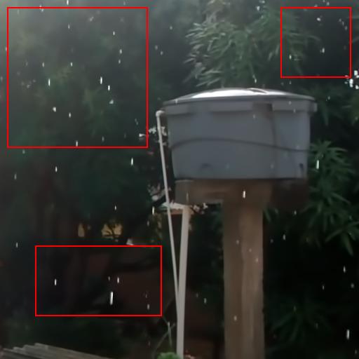
(a) Input

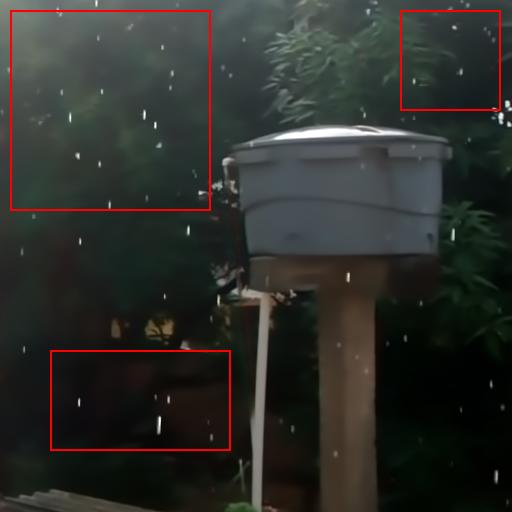
(b) PReNet

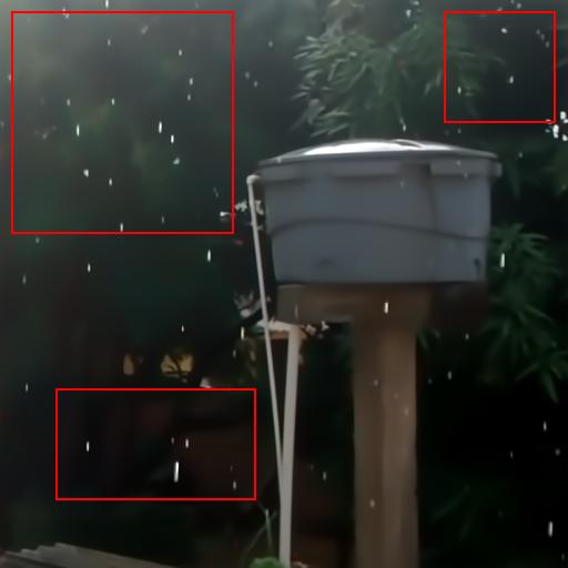
(c) M3SNet

(d) SFNet

(e) Restormer

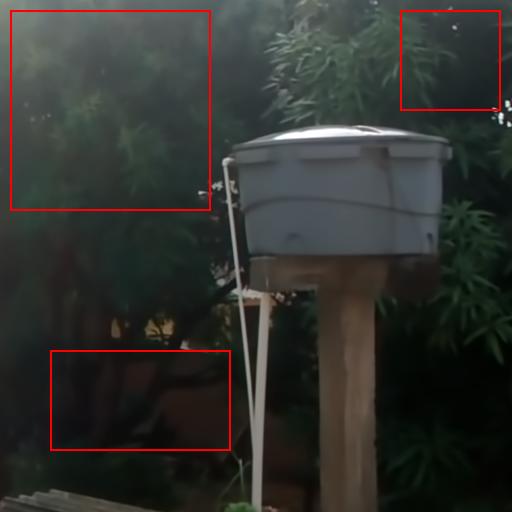
(f) Ground truth

(g) PReNet++

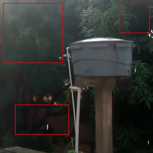
(h) M3SNet++

(i) SFNet++

(j) Restormer++

Figure 7: Visual comparison of rain removal results on a test image from SPA-Data. The first row is the input rainy image and the output of derainers trained on the original Rain1400 training set. The second row is the ground truth background image and the output of derainers trained on the Rain1400 training set augmented by our HRIGNet.

With HRIGNet, sufficient rainy images can be automatically generated from background images and rain layer masks, enabling us to create new paired rainy image datasets or augment existing datasets. In this subsection, we use HRIGNet to augment the existing datasets with ratio 1, further improving the deraining performance of current DL-based derainers on real rain datasets.

We evaluate the effectiveness of the augmentation strategy benefitted from HRIGNet with latest DL-based SIRR methods, including PReNet [6], M3SNet [4], SFNet [5] and Restormer [3]. The training sets are common synthetic datasets, including RainTrainL [14] and Rain1400 [50]. We augment these datasets, retrain the derainers and compare their generalization performance on the real dataset SPA-Data [28].

The quantitative comparison is shown in Table VI, where “+” denotes the augmented training with physics-based rendering [1] (where we use to produce rain layer masks for our HRIGNet) and “++” denotes the augmented training with our method. $\Delta\uparrow$ represents the performance gain brought by the augmented training with our method. As seen, our method improves the performance of all derainers to varying degrees. Fig. 7 shows the visual comparison of rain removal results on a test image from SPA-Data. Under such a complex rain scene, these derainers with augmented training evidently remove rains. The results validate that the rainy scene images generated by HRIGNet can help improve the robustness of these deep derainers to rainy images in the real world.

VI Conclusion And Limitations

We propose a practical two-stage learning-from-rendering pipeline for high-resolution rainy image synthesis, which combines the benefits of the realism of rendering-based methods and the high-efficiency of learning-based methods, providing the possibility of creating large-scale high-quality paired rainy-clean image datasets. In the rendering stage, we create a HRI dataset, which contains realistic high-resolution paired rainy-clean images of multiple scenes and various illumination conditions. In the learning stage, we propose a HRIGNet, which is designed to introduce a guiding diffusion model in the LDM. Experiments show that our model achieves SOTA results in most of the metrics compared to baseline image generative models. Additionally, our model is able to synthesize high-resolution rainy images up to $2048\times 1024$ resolution. Rain removal experiments on real dataset validate that our method can help improve the robustness of deep derainers to rainy images in the real world.

Although our proposed method provides the possibility of creating large-scale high-quality paired rainy-clean image datasets, there are still avenues for further improvements. Our proposed learning-from-rendering pipeline combines the two stages via rainy image datasets, which makes it less efficient in the early stage of dataset creation. In future work, we would like to integrate the two stages more effectively. In addition, in rainy images, we only consider the most common rain streak phenomenon, neglecting phenomena such as splashes and wet ground in the scene, which may also have an impact on the performance of derainers. In our rainy image rendering algorithm, for simplicity, we only render the nearest rain streaks, which can cover most of the rain streaks in the scene, but there may be some rain streaks overlapping at the same pixel position. In the future, we will attempt to use order-independent transparency rendering algorithms for optimization. Furthermore, our HRIGNet generates rainy images using rain layer masks as input. In the future, we will attempt to combine it with a DL-based rain streak generator to generate diverse and non-repetitive rain streaks in the rainy images.

Appendix A Raindrop Simulation

In atmospheric modelling, scientists usually quantify rain using a parameter called intensity of rain, $I$. It is the volume of water [36] delivered to the ground per unit of ground surface and per unit of time:

$$I=\frac{\textit{Volume of water}}{\textit{Surface of precipitation}\times\textit{duration}}.$$ (7)

In the international system of units, the intensity of rain $I$ is in $m\cdot s^{-1}$. Now, in the literature, the intensity of rain is often expressed in $mm\cdot h^{-1}$. The conversion between two units can be expressed as:

$$I=x(mm/h)=x\times\frac{10^{-3}}{3600}(m/s).$$ (8)

Raindrop size distributions. Let $D$ denote the diameter of raindrops. The number concentration of raindrops with a diameter between $D$ and $D+dD$ is then:

$$dC(D)=N(D)dD,$$ (9)

where, $N(D)$ is the raindrop size distribution (RSD). In the meteorological studies, exponential functions are often used to fit the observed RSDs.

$$N(D)=Ae^{-\beta D}$$ (10)

The exponential RSD of Marshall and Palmer [38] is one of the simplest and the most often used parameterisation to fit the RSDs:

$$N(D)=8\times 10^{6}e^{-4100I^{-0.21}D}.$$ (11)

In order to sample raindrops based on the RSD, the cumulative distribution function of raindrop diameters is needed. Limiting the range of raindrop diameters to $D\in[D_{min},D_{max}]$, we can get the total number of raindrops in this range as:

$$N_{total} =\int_{D_{min}}^{D_{max}}N(D)dD$$ (12)

$$=\frac{A}{\beta}(e^{-\beta D_{min}}-e^{-\beta D_{max}}).$$

So the probability density function of $D$ is:

$$P(D)=\frac{N(D)}{N_{total}}.$$ (13)

The cumulative distribution function of $D$ is:

$$F(D) =P(x\leq D)=\int_{D_{min}}^{D}P(x)dx$$ (14)

$$=\frac{\int_{D_{min}}^{D}N(x)dx}{N_{total}}=\frac{e^{-\beta D_{min}}-e^{-\beta D}}{e^{-\beta D_{min}}-e^{-\beta D_{max}}}.$$

In the implementation, based on the variable $u\in[0,1]$ obtained from sampling from a uniform random distribution, $D$ with distribution of $N(D)$ can be obtained by inverse transforming it using $F$.

Let $u=F(D)\in[0,1]$, then

$$D=F^{-1}(u)=\frac{ln[e^{-\beta D_{min}}-u(e^{-\beta D_{min}}-e^{-\beta D_{max}})]}{-\beta}.$$ (15)

Raindrop terminal velocity. It is generally assumed that the raindrops fall at their terminal velocity, whatever their position (their height) in the atmosphere. The transient period to reach that speed is then totally neglected. We use the raindrops terminal velocity given by Kessler [39]:

$$v_{t}=130D^{0.5}$$ (16)

Appendix B More Experiment Details

B-A Baselines

For the LDM model in Table III of the main paper, the initial learning rate is set as $2\times 10^{-6}$, the batch size is 1, the image size of the UNet backbone is $128\times 128$, and the model channels are 224. The first stage model and the conditioning stage model share a same VQGAN model, with the parameters of the model using pretrained vq-f4 from LDM. The training epoch of the LDM model is 99.

For the DiT model in Table III of the main paper, the initial learning rate is set as $2\times 10^{-6}$, the batch size is 1, the image size of the Transformer backbone is $128\times 128$, the patch size is 2, the hidden size is 768, the depth is 12, and the number of head is 12. The first stage model and the conditioning stage model share a same VQGAN model, with the parameters of the model using pretrained vq-f4 from LDM. The training epoch of the DiT model is 99.

For the CycleGAN model in Table III of the main paper, the initial learning rate is set as $5\times 10^{-5}$, the batch size is 2, the architecture of the generator is resnet with 9 blocks. The default configuration of CycleGAN is used for other parameter settings. The training epoch of the CycleGAN model is 200.

For the HRIGNet in Table III of the main paper, the training epoch is 98.

B-B Ablation Study

For the HRIGNet model with rainy image of size $256\times 256$ as guidance in Table IV of the main paper, the initial learning rate is set as $2\times 10^{-6}$, the batch size is 1, the image size of the UNet backbone is $128\times 128$, and the model channels are 224. The first stage model and the conditioning stage model share a same VQGAN model, with the parameters of the model using pretrained vq-f4 from LDM. For the guiding diffusion model, the image size of the UNet backbone is $64\times 64$, and the model channels are 224. The training epoch of the guiding diffusion model is 99, and the training epoch of the HRIGNet model is 88.

For the HRIGNet model with rain layer of size $256\times 256$ as guidance in Table IV of the main paper, the initial learning rate is set as $2\times 10^{-6}$, the batch size is 1, the image size of the UNet backbone is $128\times 128$, and the model channels are 224. The first stage model and the conditioning stage model share a same VQGAN model, with the parameters of the model using pretrained vq-f4 from LDM. For the guiding diffusion model, the image size of the UNet backbone is $64\times 64$, and the model channels are 224. The training epoch of the guiding diffusion model is 96, and the training epoch of the HRIGNet model is 88.

For the guiding diffusion model the HRIGNet model with rain layer of size $512\times 512$ as guidance in Table IV, the image size of the UNet backbone is $128\times 128$, and the model channels are 224. The training epoch of the guiding diffusion model is 99.

For the HRIGNet model with Transformer backbone in Table V of the main paper, the initial learning rate is set as $2\times 10^{-6}$, the batch size is 1. For the Transformer backbone, the image size is $128\times 128$, the patch size is 8, the hidden size is 384, the depth is 12, and the number of head is 12. The first stage model and the conditioning stage model share a same VQGAN model, with the parameters of the model using pretrained vq-f4 from LDM. The training epoch of the HRIGNet model is 75.

References

- [1] S. S. Halder, J.-F. Lalonde, and R. d. Charette, “Physics-based rendering for improving robustness to rain,” in Proceedings of the IEEE/CVF International Conference on Computer Vision, 2019, pp. 10 203–10 212.
- [2] Y. Li, R. T. Tan, X. Guo, J. Lu, and M. S. Brown, “Rain streak removal using layer priors,” in Proceedings of the IEEE Conference on Computer Vision and Pattern Recognition, 2016, pp. 2736–2744.
- [3] S. W. Zamir, A. Arora, S. Khan, M. Hayat, F. S. Khan, and M.-H. Yang, “Restormer: Efficient transformer for high-resolution image restoration,” in Proceedings of the IEEE/CVF Conference on Computer Vision and Pattern Recognition, 2022, pp. 5728–5739.
- [4] H. Gao, J. Yang, Y. Zhang, N. Wang, J. Yang, and D. Dang, “A mountain-shaped single-stage network for accurate image restoration,” arXiv preprint arXiv:2305.05146, 2023.
- [5] Y. Cui, Y. Tao, Z. Bing, W. Ren, X. Gao, X. Cao, K. Huang, and A. Knoll, “Selective frequency network for image restoration,” in The Eleventh International Conference on Learning Representations, 2022.
- [6] D. Ren, W. Zuo, Q. Hu, P. Zhu, and D. Meng, “Progressive image deraining networks: A better and simpler baseline,” in Proceedings of the IEEE/CVF Conference on Computer Vision and Pattern Recognition, 2019, pp. 3937–3946.
- [7] M. Hnewa and H. Radha, “Object detection under rainy conditions for autonomous vehicles: A review of state-of-the-art and emerging techniques,” IEEE Signal Processing Magazine, vol. 38, no. 1, pp. 53–67, 2020.
- [8] S. Di, Q. Feng, C.-G. Li, M. Zhang, H. Zhang, S. Elezovikj, C. C. Tan, and H. Ling, “Rainy night scene understanding with near scene semantic adaptation,” IEEE Transactions on Intelligent Transportation Systems, vol. 22, no. 3, pp. 1594–1602, 2020.
- [9] H. Wang, Z. Yue, Q. Xie, Q. Zhao, Y. Zheng, and D. Meng, “From rain generation to rain removal,” in Proceedings of the IEEE/CVF Conference on Computer Vision and Pattern Recognition, 2021, pp. 14 791–14 801.
- [10] S. Li, I. B. Araujo, W. Ren, Z. Wang, E. K. Tokuda, R. H. Junior, R. Cesar-Junior, J. Zhang, X. Guo, and X. Cao, “Single image deraining: A comprehensive benchmark analysis,” in Proceedings of the IEEE/CVF Conference on Computer Vision and Pattern Recognition, 2019, pp. 3838–3847.
- [11] K. Garg and S. K. Nayar, “Vision and rain,” International Journal of Computer Vision, vol. 75, pp. 3–27, 2007.
- [12] K. Garg and S. K. Nayar, “When does a camera see rain?” in Tenth IEEE International Conference on Computer Vision (ICCV’05) Volume 1, vol. 2. IEEE, 2005, pp. 1067–1074.
- [13] R. Quan, X. Yu, Y. Liang, and Y. Yang, “Removing raindrops and rain streaks in one go,” in Proceedings of the IEEE/CVF Conference on Computer Vision and Pattern Recognition, 2021, pp. 9147–9156.
- [14] W. Yang, R. T. Tan, J. Feng, J. Liu, Z. Guo, and S. Yan, “Deep joint rain detection and removal from a single image,” in Proceedings of the IEEE Conference on Computer Vision and Pattern Recognition, 2017, pp. 1357–1366.
- [15] K. Jiang, Z. Wang, P. Yi, C. Chen, B. Huang, Y. Luo, J. Ma, and J. Jiang, “Multi-scale progressive fusion network for single image deraining,” in Proceedings of the IEEE/CVF Conference on Computer Vision and Pattern Recognition, 2020, pp. 8346–8355.
- [16] X. Hu, C.-W. Fu, L. Zhu, and P.-A. Heng, “Depth-attentional features for single-image rain removal,” in Proceedings of the IEEE/CVF Conference on Computer Vision and Pattern Recognition, 2019, pp. 8022–8031.
- [17] K. Garg and S. K. Nayar, “Photorealistic rendering of rain streaks,” ACM Transactions on Graphics (TOG), vol. 25, no. 3, pp. 996–1002, 2006.
- [18] M. Pharr, W. Jakob, and G. Humphreys, Physically based rendering: From theory to implementation. Morgan Kaufmann, 2016.
- [19] B. O. Community, Blender - a 3D modelling and rendering package, Blender Foundation, Stichting Blender Foundation, Amsterdam, 2018. [Online]. Available: http://www.blender.org
- [20] S. Ni, X. Cao, T. Yue, and X. Hu, “Controlling the rain: From removal to rendering,” in Proceedings of the IEEE/CVF Conference on Computer Vision and Pattern Recognition, 2021, pp. 6328–6337.
- [21] Y. Wei, Z. Zhang, Y. Wang, M. Xu, Y. Yang, S. Yan, and M. Wang, “Deraincyclegan: Rain attentive cyclegan for single image deraining and rainmaking,” IEEE Transactions on Image Processing, vol. 30, pp. 4788–4801, 2021.
- [22] Y. Ye, Y. Chang, H. Zhou, and L. Yan, “Closing the loop: Joint rain generation and removal via disentangled image translation,” in Proceedings of the IEEE/CVF Conference on Computer Vision and Pattern Recognition, 2021, pp. 2053–2062.
- [23] J. Ho, A. Jain, and P. Abbeel, “Denoising diffusion probabilistic models,” Advances in Neural Information Processing Systems, vol. 33, pp. 6840–6851, 2020.
- [24] R. Rombach, A. Blattmann, D. Lorenz, P. Esser, and B. Ommer, “High-resolution image synthesis with latent diffusion models,” in Proceedings of the IEEE/CVF Conference on Computer Vision and Pattern Recognition, 2022, pp. 10 684–10 695.
- [25] W. Peebles and S. Xie, “Scalable diffusion models with transformers,” in Proceedings of the IEEE/CVF International Conference on Computer Vision, 2023, pp. 4195–4205.
- [26] D. Liu, S. Shetty, T. Hinz, M. Fisher, R. Zhang, T. Park, and E. Kalogerakis, “Asset: autoregressive semantic scene editing with transformers at high resolutions,” ACM Transactions on Graphics (TOG), vol. 41, no. 4, pp. 1–12, 2022.
- [27] A. Vaswani, N. Shazeer, N. Parmar, J. Uszkoreit, L. Jones, A. N. Gomez, Ł. Kaiser, and I. Polosukhin, “Attention is all you need,” Advances in Neural Information Processing Systems, vol. 30, 2017.
- [28] T. Wang, X. Yang, K. Xu, S. Chen, Q. Zhang, and R. W. Lau, “Spatial attentive single-image deraining with a high quality real rain dataset,” in Proceedings of the IEEE/CVF Conference on Computer Vision and Pattern Recognition, 2019, pp. 12 270–12 279.
- [29] M. Cordts, M. Omran, S. Ramos, T. Rehfeld, M. Enzweiler, R. Benenson, U. Franke, S. Roth, and B. Schiele, “The cityscapes dataset for semantic urban scene understanding,” in Proceedings of the IEEE Conference on Computer Vision and Pattern Recognition, 2016, pp. 3213–3223.
- [30] I. Goodfellow, J. Pouget-Abadie, M. Mirza, B. Xu, D. Warde-Farley, S. Ozair, A. Courville, and Y. Bengio, “Generative adversarial networks,” Communications of the ACM, vol. 63, no. 11, pp. 139–144, 2020.
- [31] J.-Y. Zhu, T. Park, P. Isola, and A. A. Efros, “Unpaired image-to-image translation using cycle-consistent adversarial networks,” in Proceedings of the IEEE International Conference on Computer Vision, 2017, pp. 2223–2232.
- [32] D. P. Kingma and M. Welling, “Auto-encoding variational bayes,” arXiv preprint arXiv:1312.6114, 2013.
- [33] G. Batzolis, J. Stanczuk, C.-B. Schönlieb, and C. Etmann, “Conditional image generation with score-based diffusion models,” arXiv preprint arXiv:2111.13606, 2021.
- [34] Z. Yi, Q. Tang, S. Azizi, D. Jang, and Z. Xu, “Contextual residual aggregation for ultra high-resolution image inpainting,” in Proceedings of the IEEE/CVF Conference on Computer Vision and Pattern Recognition, 2020, pp. 7508–7517.
- [35] C. Zheng, T.-J. Cham, J. Cai, and D. Phung, “Bridging global context interactions for high-fidelity image completion,” in Proceedings of the IEEE/CVF Conference on Computer Vision and Pattern Recognition, 2022, pp. 11 512–11 522.
- [36] N. Duhanyan and Y. Roustan, “Below-cloud scavenging by rain of atmospheric gases and particulates,” Atmospheric Environment, vol. 45, no. 39, pp. 7201–7217, 2011.
- [37] M. Mircea and S. Stefan, “A theoretical study of the microphysical parameterization of the scavenging coefficient as a function of precipitation type and rate,” Atmospheric Environment, vol. 32, no. 17, pp. 2931–2938, 1998.
- [38] A. Best, “The size distribution of raindrops,” Quarterly Journal of the Royal Meteorological Society, vol. 76, no. 327, pp. 16–36, 1950.
- [39] E. Kessler, “On the distribution and continuity of water substance in atmospheric circulations,” in On the Distribution and Continuity of Water Substance in Atmospheric Circulations. Springer, 1969, pp. 1–84.
- [40] A. Dosovitskiy, L. Beyer, A. Kolesnikov, D. Weissenborn, X. Zhai, T. Unterthiner, M. Dehghani, M. Minderer, G. Heigold, S. Gelly et al., “An image is worth 16x16 words: Transformers for image recognition at scale,” arXiv preprint arXiv:2010.11929, 2020.
- [41] O. Ronneberger, P. Fischer, and T. Brox, “U-net: Convolutional networks for biomedical image segmentation,” in Medical Image Computing and Computer-Assisted Intervention–MICCAI 2015: 18th International Conference, Munich, Germany, October 5-9, 2015, Proceedings, Part III 18. Springer, 2015, pp. 234–241.
- [42] P. Esser, R. Rombach, and B. Ommer, “Taming transformers for high-resolution image synthesis,” in Proceedings of the IEEE/CVF Conference on Computer Vision and Pattern Recognition, 2021, pp. 12 873–12 883.
- [43] D. P. Kingma and J. Ba, “Adam: A method for stochastic optimization,” arXiv preprint arXiv:1412.6980, 2014.
- [44] I. Loshchilov and F. Hutter, “Decoupled weight decay regularization,” arXiv preprint arXiv:1711.05101, 2017.
- [45] A. Paszke, S. Gross, F. Massa, A. Lerer, J. Bradbury, G. Chanan, T. Killeen, Z. Lin, N. Gimelshein, L. Antiga et al., “Pytorch: An imperative style, high-performance deep learning library,” Advances in Neural Information Processing Systems, vol. 32, 2019.
- [46] M. Heusel, H. Ramsauer, T. Unterthiner, B. Nessler, and S. Hochreiter, “Gans trained by a two time-scale update rule converge to a local nash equilibrium,” Advances in Neural Information Processing Systems, vol. 30, 2017.
- [47] R. Zhang, P. Isola, A. A. Efros, E. Shechtman, and O. Wang, “The unreasonable effectiveness of deep features as a perceptual metric,” in Proceedings of the IEEE Conference on Computer Vision and Pattern Recognition, 2018, pp. 586–595.
- [48] Z. Wang, A. C. Bovik, H. R. Sheikh, and E. P. Simoncelli, “Image quality assessment: from error visibility to structural similarity,” IEEE Transactions on Image Processing, vol. 13, no. 4, pp. 600–612, 2004.
- [49] A. Hore and D. Ziou, “Image quality metrics: Psnr vs. ssim,” in 2010 20th International Conference on Pattern Recognition. IEEE, 2010, pp. 2366–2369.
- [50] X. Fu, J. Huang, D. Zeng, Y. Huang, X. Ding, and J. Paisley, “Removing rain from single images via a deep detail network,” in Proceedings of the IEEE Conference on Computer Vision and Pattern Recognition, 2017, pp. 3855–3863.