TabGen-ICL: Residual-Aware In-Context Example Selection for Tabular Data Generation

Abstract

Large Language models (LLMs) have achieved encouraging results in tabular data generation. However, existing approaches require fine-tuning, which is computationally expensive. This paper explores an alternative: prompting a fixed LLM with in-context examples. We observe that using randomly selected in-context examples hampers the LLM’s performance, resulting in sub-optimal generation quality. To address this, we propose a novel in-context learning framework: TabGen-ICL, to enhance the in-context learning ability of LLMs for tabular data generation. TabGen-ICL operates iteratively, retrieving a subset of real samples that represent the residual between currently generated samples and true data distributions. This approach serves two purposes: locally, it provides more effective in-context learning examples for the LLM in each iteration; globally, it progressively narrows the gap between generated and real data. Extensive experiments on five real-world tabular datasets demonstrate that TabGen-ICL significantly outperforms the random selection strategy. Specifically, it reduces the error rate by a margin of $3.5\%-42.2\%$ on fidelity metrics. We demonstrate for the first time that prompting a fixed LLM can yield high-quality synthetic tabular data. The code is provided in the link.

TabGen-ICL: Residual-Aware In-Context Example Selection for Tabular Data Generation

Liancheng Fang ¹, Aiwei Liu ², Hengrui Zhang ¹, Henry Peng Zou ¹, Weizhi Zhang¹, Philip S. Yu¹, ¹University of Illinois Chicago, ²Tsinghua University, lfang87@uic.edu, liuaw20@mails.tsinghua.edu.cn, psyu@uic.edu

1 Introduction

Tabular data, despite being one of the most prevalent data modalities in real-world applications (Benjelloun et al., 2020), often encounters several issues in practical use. These include imbalanced data categories (Cao et al., 2019), privacy concerns (Gascón et al., 2016) (as many tabular datasets contain sensitive personal information that cannot be directly shared), insufficient data quality Lin and Tsai (2020), and high data collection costs (Even et al., 2007). Tabular generation is an important means to address these problems. Classic tabular generation methods such as GANs (Xu et al., 2019), VAEs (Liu et al., 2023), and diffusion models (Kim et al., 2023; Lee et al., 2023; Kotelnikov et al., 2023; Zhang et al., 2024) have two main limitations. First, they require large amounts of tabular data for training, which leads to a noticeable decline in performance in low-resource scenarios. This is particularly problematic considering that most real-world situations requiring tabular generation lack abundant data. Second, they need special preprocessing to handle heterogeneous data types, making them less flexible.

The rapid development of large language models (LLMs) brings new possibilities for solving table data generation problems with their powerful semantic understanding, reasoning, and generation capabilities. LLMs can understand and process various data types and structures without complicated data preprocessing, offering more flexible and principled solutions. Moreover, LLMs’ few-shot learning ability may alleviate data scarcity issues, enabling excellent performance in low-resource scenarios. Previous works (Borisov et al., 2023; Solatorio and Dupriez, 2023; Zhang et al., 2023; Zhao et al., 2023; Gulati and Roysdon, 2023; Xu et al., 2024a; Wang et al., 2024) resort to fine-tuning general-purpose LLMs on target tables. While effective, fine-tuning requires substantial computational resources, making it inapplicable in resource-scarce scenarios.

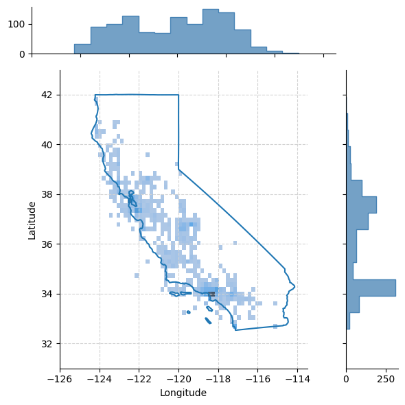
(a) No in-context Ex.

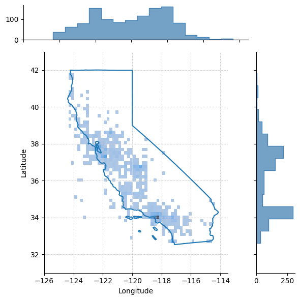
(b) Sampled in-context Ex.

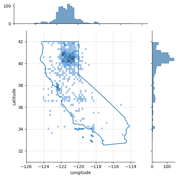
(c) Fixed in-context Ex.

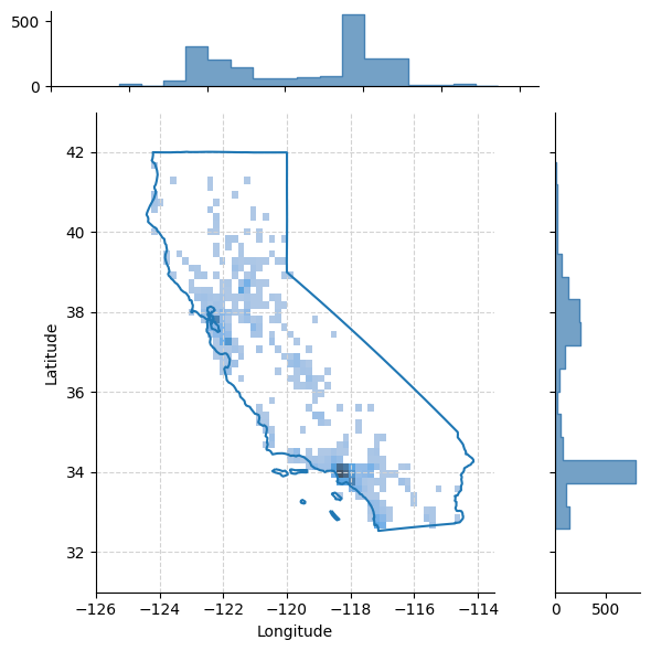
(d) Ground Truth

Figure 1: Comparison of samples generated with different in-context learning examples. Plots show the latitude and longitude coordinates of California housing, with the solid line representing the state boundary. (a) 2000 samples generated by LLM with only the table header as input, without any in-context examples. (b) 2000 samples generated by LLM, giving in-context examples sampled from the real dataset. (c) 2000 synthetic samples generated by LLM, giving in-context examples with latitude and longitude in a fixed range. (d) 2000 samples from the ground truth training table.

In-context learning effectively solves such problems. By adding examples to the context, distribution characteristics can be provided to LLMs, guiding them to generate data that conforms to the target distribution without specific fine-tuning (Gao et al., 2023). However, simple in-context learning strategies still face challenges. Figure 1(a) shows that even without in-context examples (see the full prompt at Appendix A.2), LLMs can generate reasonable distributions, reflecting the influence of the LLM’s pre-training distribution. Figure 1(b) demonstrates the strategy proposed by (Seedat et al., 2024), which involves random sampling from Ground Truth as in-context examples. Although the generated results are closer to the Ground Truth shown in Figure 1(d) compared to Figure 1(a), they are still mainly influenced by the LLM’s original distribution and struggle to fit the Ground Truth.

This phenomenon reveals the importance of choosing in-context examples. In this work, we propose TabGen-ICL, a dynamic in-context example selection method. Inspired by the observation in Figure 1(c), we found that using fixed range in-context examples leads to generated distributions closely mimicking those examples, significantly differing from the LLM’s original distribution. This indicates in-context learning’s ability to simulate distributions. By carefully selecting in-context examples, we can more effectively guide LLMs to generate distributions closer to the ground truth.

Central to our framework is the design of an automated strategy for selecting effective in-context examples while ensuring global consistency with the real data distribution. Our key idea is to utilize simple, discernible patterns in subsets of real samples, which can effectively guide LLMs in generating realistic tabular data. Specifically, TabGen-ICL identifies subsets of real samples that exhibit simple patterns and closely match the residual between the current generated data distribution and the real data distribution. This idea can be categorized as a novel residual-aware RAG technique, where we retrieve in-context examples based on the residual between the generated and real data distributions.

The residual-aware sampling measures the discrepancy between the generated and real data distributions, focusing on areas where the model needs improvement. This approach enables TabGen-ICL to progressively narrow the distribution gap while maintaining the use of easily learnable patterns in the in-context examples. Our sampling technique offers two key advantages: flexibility in selecting simple patterns for effective learning, and consistent generation through progressive distribution alignment. The contributions of this paper are as follows:

1. We propose TabGen-ICL, an in-context learning selection method that retrieves in-context examples by leveraging residual between currently generated samples and true data distributions.

2. We conduct extensive experiments on five datasets, evaluated under three distinct groups of synthetic data evaluation metrics. Experiment results show that TabGen-ICL outperforms the previous in-context learning method by a margin of $3.5\%-42.2\%$ across multiple fidelity metrics. Notably, TabGen-ICL surpasses state-of-the-art deep generative models under the data-scarce scenarios.

2 Related works

Deep generative models for synthetic tabular data generation

Generative models for tabular data have become increasingly important and have widespread applications Assefa et al. (2021); Zheng and Charoenphakdee (2022); Hernandez et al. (2022). For example, CTGAN and TAVE (Xu et al., 2019) deal with mixed-type tabular data generation using the basic GAN (Goodfellow et al., 2014) and VAE (Kingma and Welling, 2013) framework. GOGGLE (Liu et al., 2023) incorporates Graph Attention Networks in a VAE framework such that the correlation between different data columns can be explicitly learned. Recently, inspired by the success of Diffusion models in image generation, a lot of diffusion-based methods have been proposed, such as TabDDPM (Kotelnikov et al., 2023), STaSy (Kim et al., 2023), CoDi (Lee et al., 2023), and TabSyn (Zhang et al., 2024).

LLMs for synthetic data generation.

Collecting high-quality training data for advanced deep-learning models is often costly and time-consuming. Researchers have recently explored using pre-trained large language models (LLMs) to generate synthetic datasets as a promising alternative. While LLMs have shown proficiency in generating high-quality synthetic text data, their ability to accurately replicate input data distributions at scale remains uncertain (Xu et al., 2024b). Studies like Curated-LLM (Seedat et al., 2024) demonstrate LLMs’ effectiveness in augmenting tabular data in low-data scenarios, but their application to large-scale input data is still unclear. GReaT (Borisov et al., 2023), another approach using GPT-2, generates synthetic tabular data but requires fine-tuning for each new dataset.

3 Preliminaries

Notation.

Tabular dataset refers to data organized in a tabular format with $N$ row and $D$ columns, where each row denotes a data record or sample, and each column denotes an attribute or feature. Each attribute can be either discrete (e.g. categorical) or continuous (e.g. real number $\mathbb{R}$). We use $\mathbb{P}(\boldsymbol{x})$ to denote the probability distribution of $\boldsymbol{x}$.

Data Setup.

We have access to a training dataset of $N$ samples: $\mathcal{D}_{train}=\{\boldsymbol{x}_{i}\}_{i=1}^{N}$, each sample $\boldsymbol{x}_{i}$ is i.i.d. drawn from an unknown distribution $\mathbb{P}(\boldsymbol{x})$.

Objective.

The goal is to generate a new dataset $\mathcal{D}_{syn}=\{\hat{\boldsymbol{x}}_{i}\}_{i=1}^{N}$ such that $\hat{\boldsymbol{x}}_{i}$ is i.i.d. sampled from $\mathbb{P}(\boldsymbol{x})$. Direct copy of training data is not allowed.

Serialization.

As LLMs primarily process text input, it is necessary to convert tabular data into a suitable textual format. There are many serialization formats for tabular data, such as JSON (Singha et al., 2023), Markdown (Sui et al., 2024), Sentences (Borisov et al., 2023), etc. Notably, the JSON format is widely supported by LLMs, with models like GPT-4o capable of generating structured outputs in JSON format through constrained decoding (Liu et al., 2024). Therefore, in this study, we adopt a JSON format to serialize tabular data. For instance, a row from a table containing three columns—name (categorical), age (numerical), and city (categorical)—is transformed into a JSON object: $\{\texttt{{name:`Alice', age:25, city:`New York'}}\}$. For a table comprising $N$ rows, the serialized data becomes a list of $N$ JSON objects. See Appendix A.3 for the implementation of the JSON schema. During each prompting iteration, TabGen-ICL retrieves a subset of these JSON objects to serve as in-context examples. This process will be elaborated upon in subsequent sections.

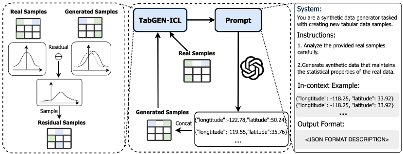
Figure 2: Overview of TabGen-ICL framework. We generate synthetic samples in batches, at each prompt iteration, TabGen-ICL retrieves a subset of real samples that acts as a residual between the currently generated samples and the real data. The residual samples will be used as in-context examples to prompt LLMs in the next iteration. The full prompt template is available in the Appendix A.1.

4 TabGen-ICL

This section presents TabGen-ICL framework for tabular data generation. TabGen-ICL retrieves a subset of samples from the training dataset that satisfy two properties: 1) Local: at each prompting iteration, the LLMs can effectively extract patterns from the in-context examples; 2) Global: after enough iterations, the overall generated samples mimic the distribution of the real samples. In the following, we will introduce each component of TabGen-ICL in detail.

4.1 LLM Generation with In-context Examples

Our key observation is LLMs have strong prior distribution, and LLMs tend to generate samples following their prior distribution, neglecting the in-context examples, see Figure 1. Formally, given in-context examples, we assume the LLMs generate samples following a mixture distribution:

Definition 1 (LLM Generation Distribution).

Given the empirical distribution of in-context example: $\mathbb{P}_{ic}$. We define the LLMs generation distribution to be the following mixture of distributions:

$$\mathbb{P}_{gen}:=\lambda\mathbb{P}_{llm}+(1-\lambda)\mathbb{P}_{ic}$$ (1)

where $\mathbb{P}_{llm}$ is the prior distribution of LLMs, $\lambda\in[0,1]$. To sample from $\mathbb{P}_{gen}$, we first sample an index $z$ from a categorical distribution over $\{0,1\}$ with parameter $\lambda$, then sample from the corresponding distribution:

$$\mathbb{P}_{gen}(\boldsymbol{x})=\begin{cases}\mathbb{P}_{llm}(\boldsymbol{x})&\text{if }z=1\\ \mathbb{P}_{ic}(\boldsymbol{x})&\text{if }z=0\end{cases}$$

Definition 1 quantifies how the in-context examples steer the LLMs’ generation from its own prior distribution towards the target distribution. Intuitively, the more in-context examples being provided, $\lambda$ will be closer to $0$, meaning the LLMs is more likely to generate samples following the empirical distribution of in-context examples. In practice, due to the limited context window of LLMs, only a small number of in-context examples can be provided, thus we expect $\lambda$ to be close to $1$.

4.2 In-context Examples Selection

Recall our goal is to let LLMs generate samples that follow the same distribution as the training table, i.e. $\mathbb{P}_{gen}\approx\mathbb{P}_{train}$. It is tempting to choose the in-context examples by sampling from the empirical distribution of the training table, i.e. $\mathbb{P}_{ic}=\mathbb{P}_{train}$ (Seedat et al., 2024). However, as the LLMs’ generation is affected by the prior distribution $\mathbb{P}_{llm}$, the actual output distribution of LLMs would be $\mathbb{P}_{gen}=\lambda\mathbb{P}_{llm}+(1-\lambda)\mathbb{P}_{train}$, which is not our target distribution $\mathbb{P}_{train}$. Instead, a more plausible way is to select in-context examples s.t., when combined with $\lambda$ proportion of data generated from $\mathbb{P}_{llm}$, the resulting distribution is close to $\mathbb{P}_{train}$. In other words, the in-context examples can be understood as the residual of $\mathbb{P}_{train}$ w.r.t. $\mathbb{P}_{llm}$. Formally, we introduce the definition of residual as follows:

Definition 2 (Residual).

Let $\boldsymbol{X}$ be a set of $N$ $i.i.d.$ samples from a data distribution $\mathbb{P}(\boldsymbol{x})$, and let $\boldsymbol{Y}$ be an arbitrary set of samples with the same dimension as $\boldsymbol{X}$. We define the residual (abbrev. RES) of $\boldsymbol{X}$ w.r.t. $\boldsymbol{Y}$ as a subset of $n$ samples of $\boldsymbol{X}$ such that, when concatenated with $\boldsymbol{Y}$, the empirical distribution of the concatenated samples is most similar to the data distribution $\mathbb{P}(\boldsymbol{x})$:

$$\texttt{RES}(\boldsymbol{X},\boldsymbol{Y},n):=\mathop{\arg\min}_{\boldsymbol{X}^{\prime}\subseteq\boldsymbol{X},|\boldsymbol{X}^{\prime}|=n}d(\boldsymbol{X},\boldsymbol{Y}\cup\boldsymbol{X}^{\prime})$$ (2)

where $d$ can be any distance metric between two empirical distributions.

Remark 1.

In our case, $\boldsymbol{X}$ is the real tabular samples, and $\boldsymbol{Y}$ is the current generated samples by a LLM. Intuitively, the residual samples capture the part of the real samples that LLM has not yet grasped, thus named as residual. To prevent overly long context prompts when interacting with the LLM, we enforce an upper-bound $n$ on the size of the residual samples. In our experiments, we set $n=500$ and instantiate $d$ as Jensen-Shannon Divergence (JSD) and Kolmogorov-Smirnov Distance (KSD).

Since brute-force way of computing the residual is computationally prohibitive for large $N$ and $n$, we introduce a heuristic for sampling the residual. We describe details in the following—pseudo-code is provided in Appendix 1.

4.3 Compute Residual

We propose to use a simple heuristic to shrink the search space. Specifically, we first randomly select a column, then we group the real samples $\boldsymbol{X}$ based on the value of the selected column. Each group of samples is then concatenated with the generated samples $\boldsymbol{Y}$. Finally, we select the group that has the smallest distance to the real samples $\boldsymbol{X}$ as the residual. The time complexity of this heuristic search algorithm is $O(N)$. Additionally, the final residual subset always exhibits a consistent pattern—either sharing the same category or falling within a narrow numerical range in one of its columns. We hypothesize that this simple pattern makes the residual samples particularly effective as in-context examples for LLMs (see Figure 1 (c)).

	Method	Marginal$\downarrow\%$	Corr$\downarrow\%$	Precision$\downarrow\%$	Recall$\downarrow\%$	C2ST$\downarrow\%$	JSD$\downarrow 10^{-2}$
VAE-based
	TVAE (Xu et al., 2019)	$14.61$	$17.32$	$11.65$	$9.11$	$41.72$	$0.63$
GAN-based
	CTGAN (Xu et al., 2019)	$16.36$	$20.33$	$30.65$	$11.41$	$42.90$	$0.91$
Diffusion-based
	STaSy (Kim et al., 2023)	$12.35$	$9.72$	$11.09$	$2.66$	$55.82$	$1.34$
	CoDi (Lee et al., 2023)	$21.70$	$24.92$	$9.89$	$6.74$	$57.88$	$1.07$
	TabDDPM (Kotelnikov et al., 2023)	$14.04$	$8.16$	$13.37$	$2.27$	$24.21$	$0.85$
	TabSyn (Zhang et al., 2024)	$1.40$	$2.36$	$3.76$	$2.29$	$2.64$	$0.05$
Autoregressive Models
	RTF (Solatorio and Dupriez, 2023)	$5.31$	$10.42$	$3.53$	$5.25$	$28.16$	$0.45$
	TabMT (Gulati and Roysdon, 2023)	$4.46$	$8.24$	$33.88$	$50.44$	$44.77$	$0.63$
LLM-Finetuned
	GReaT (Borisov et al., 2023)	$15.53$	$40.48$	$1.49$	$10.06$	$48.28$	$1.06$
LLM-Prompt-Only
	CLLM w. GPT-4o-mini	$13.17$	$19.57$	$6.63$	$8.08$	$39.02$	$0.78$
	TabGen-ICL w. GPT-4o-mini (Ours)	$11.39$	$17.07$	$5.54$	$4.67$	$37.63$	$0.80$
	Improvement	$\bf{{\color[rgb]{0.8,0.25,0.1}13.5\%}}$	$\bf{{\color[rgb]{0.8,0.25,0.1}12.8\%}}$	$\bf{{\color[rgb]{0.8,0.25,0.1}19.7\%}}$	$\bf{{\color[rgb]{0.8,0.25,0.1}42.2\%}}$	$\bf{{\color[rgb]{0.8,0.25,0.1}3.5\%}}$	$-$
	CLLM w. GPT-4o	$10.57$	$13.46$	$4.00$	$4.25$	$31.51$	$0.63$
	TabGen-ICL w. GPT-4o (Ours)	$9.14$	$12.86$	$4.93$	$2.80$	$26.70$	$0.62$
	Improvement	$\bf{{\color[rgb]{0.8,0.25,0.1}13.6\%}}$	$\bf{{\color[rgb]{0.8,0.25,0.1}4.5\%}}$	$-$	$\bf{{\color[rgb]{0.8,0.25,0.1}34.1\%}}$	$\bf{{\color[rgb]{0.8,0.25,0.1}15.3\%}}$	$\bf{{\color[rgb]{0.8,0.25,0.1}1.6\%}}$

Table 1: Fidelity comparison: Comparison of various methods on fidelity metrics. Results are averaged over all datasets. All metrics are scaled to percentages ($\%$) or $10^{-2}$, and reversed so that the lower the better.

4.4 Table Generation by TabGen-ICL

TabGen-ICL can be easily integrated with LLMs to generate high-quality synthetic tabular data. See Fig. 2 for an overview of the procedure. Here are the concrete steps involved in this procedure:

1. In-context Prompting: For the first iteration, we randomly select $n$ samples from the real dataset $\boldsymbol{X}$ as the initial set of in-context examples. Otherwise, we plug the residual samples computed in the previous iteration into the prompt template to prompt LLMs. We append the generated samples into $\boldsymbol{Y}$.

2. Residual Computation: We then compute the residual of $\boldsymbol{X}$ w.r.t. $\boldsymbol{Y}$: $\texttt{RES}(\boldsymbol{X},\boldsymbol{Y},n)$. Specifically, if the current iteration is an even number, we instantiate $d$ as JSD, otherwise, we instantiate $d$ as KSD.

3. Iterative Refinement: Repeat the above steps until enough synthetic samples are generated.

5 Experiments

We validate the performance of TabGen-ICL through extensive experiments. In particular, we investigate the following questions:

• Can TabGen-ICL improve generation quality compared to previous LLM-based methods? (Table. 1, 2, Fig. 5)

• How does TabGen-ICL perform, compared to training-based deep generative models, under a data-scarcity setting? (Fig. 3)

• Does TabGen-ICL generate new synthetic data instead of copying the training dataset? (Fig. 4)

5.1 Setup

Datasets.

We select five real-world tabular datasets containing both numerical and categorical attributes: Adult, Default, Shoppers, Magic and California. The statistics of the datasets are summarized in Table 5 in Appendix A.5.

Baselines.

To comprehensively assess TabGen-ICL’s performance, we conduct comparisons against a wide range of traditional deep generative models and LLM-based methods, which we categorize into the following two groups:

• Deep generative models: 1) VAE-based method TVAE (Xu et al., 2019), 2) GAN-based method CTGAN (Xu et al., 2019), 3) Diffusion-based method TabSyn (Zhang et al., 2024), TabDDPM (Kotelnikov et al., 2023), CoDi (Lee et al., 2023), STaSy (Kim et al., 2023), 4) Autoregressive method TabMT (Gulati and Roysdon, 2023), RealTabformer (RTF) (Solatorio and Dupriez, 2023).

• LLM-based methods: 1) with fine-tuning: GReaT (Borisov et al., 2023) 2) without fine-tuning: CLLM Seedat et al. (2024). CLLM was originally employed with GPT-3.5 and GPT-4, to ensure a fair comparison to CLLM, we employ CLLM with stronger models: GPT-4o-mini and GPT-4o, and we keep all the other experimental settings the same as ours.

To the best of our knowledge, CLLM Seedat et al. (2024) is the only previous work that is training-free and solely based on in-context learning (excluding the curation step). TabGen-ICL falls in this setting.

Implementation details.

Our main experiments employ GPT-4o-mini and GPT-4o as the LLMs. For all LLMs, we set the temperature to $1.0$. We generate 3000 samples ($N=3000$) for each dataset. Each experiment is conducted 5 times and the average results are reported.

Evaluation metrics.

We evaluate the synthetic tabular data from three distinct dimensions: Fidelity - if the synthetic data faithfully recovers the ground-truth data distribution. We evaluate fidelity by 5 metrics: 1) Marginal distribution through Kolmogorov-Sirnov Test, 2) Pair-wise column correlation (Corr.) by computing Pearson Correlation, 3) Classifier Two Sample Test (C2ST) 4) Precision and Recall, 5) Jensen-Shannon Divergence (JSD). Utility - the utility of the synthetic data when used to train downstream models, we use the Train-on-Synthetic-then-Test (TSTR) protocol to evaluate the AUC score of XGBoost model on predicting the target column of each dataset. Privacy - if the synthetic data is not copied from the real records, we employ the Distance to Closest Record (DCR) metric. We defer the full description of the metrics to Appendix A.6.

Notably, previous works (Borisov et al., 2023; Seedat et al., 2024) on evaluating LLMs for tabular data generation focus only on Machine Learning Utility and Privacy protection. Our paper fills this gap by providing the first comprehensive evaluation of LLMs’ ability on tabular data synthesis.

	Method	California	Adult	Shoppers	Magic	Default
		AUC$\uparrow$	AUC$\uparrow$	AUC$\uparrow$	AUC$\uparrow$	AUC$\uparrow$
	Real	$0.999$	$0.927$	$0.926$	$0.946$	$0.770$
VAE-based
	TVAE (Xu et al., 2019)	$0.986$	$0.846$	$0.898$	$0.912$	$0.744$
GAN-based
	CTGAN (Xu et al., 2019)	$0.925$	$0.874$	$0.868$	$0.874$	$0.736$
Diffusion-based
	STaSy (Kim et al., 2023)	$0.997$	$0.903$	$0.909$	$0.923$	$0.749$
	CoDi (Lee et al., 2023)	$0.981$	$0.829$	$0.855$	$0.930$	$0.497$
	TabDDPM (Kotelnikov et al., 2023)	$0.992$	$0.911$	$0.915$	$0.933$	$0.763$
	TabSyn (Zhang et al., 2024)	$0.993$	$0.904$	$0.913$	$0.934$	$0.764$
Autoregressive Models
	RTF (Solatorio and Dupriez, 2023)	$0.948$	$0.925$	$-$	$0.931$	$0.764$
	TabMT (Gulati and Roysdon, 2023)	$0.988$	$0.873$	$0.912$	$0.822$	$0.714$
LLM-Finetuned
	GReaT (Borisov et al., 2023)	$0.996$	$0.913$	$0.902$	$0.888$	$0.755$
LLM-Prompt-Only
	CLLM w. GPT-4o-mini	$0.840$	$0.879$	$0.708$	$0.826$	$0.557$
	TabGen-ICL w. GPT-4o-mini (Ours)	$0.947$	$0.894$	$0.792$	$0.891$	$0.628$
	Improvement	$\bf{{\color[rgb]{0.8,0.25,0.1}12.7\%}}$	$\bf{{\color[rgb]{0.8,0.25,0.1}1.7\%}}$	$\bf{{\color[rgb]{0.8,0.25,0.1}11.9\%}}$	$\bf{{\color[rgb]{0.8,0.25,0.1}7.9\%}}$	$\bf{{\color[rgb]{0.8,0.25,0.1}12.7\%}}$
	CLLM w. GPT-4o	$0.947$	$0.891$	$0.865$	$0.885$	$0.718$
	TabGen-ICL w. GPT-4o (Ours)	$0.975$	$0.892$	$0.879$	$0.903$	$0.713$
	Improvement	$\bf{{\color[rgb]{0.8,0.25,0.1}3.0\%}}$	$\bf{{\color[rgb]{0.8,0.25,0.1}0.1\%}}$	$\bf{{\color[rgb]{0.8,0.25,0.1}1.4\%}}$	$\bf{{\color[rgb]{0.8,0.25,0.1}1.8\%}}$	$\bf{{\color[rgb]{0.8,0.25,0.1}0.5\%}}$

Table 2: Utility comparison: AUC scores of Train-on-synthetic-Test-on-real (TSTR) XGBoost model predicting the target column of each table. $\uparrow$ indicates the higher the better. $-$ indicates training failure.

5.2 TabGen-ICL outperforms LLM-based baseline methods

As shown in Table 1, TabGen-ICL consistently outperforms current LLM-based approaches on fidelity metrics, including both the training-free method CLLM and the fine-tuning-based method GReaT. Specifically, when using GPT-4o-mini, TabGen-ICL improves fidelity scores by a margin of 3.5$\%\textendash 42.2\%$, and when using GPT-4o, the improvements range from $1.6\%$ to 34.1% across various metrics. Notably, the highest gains are observed in Recall: 42.2% improvement with GPT-4o-mini and 34.1% with GPT-4o. Recall measures whether the synthetic data adequately covers the diverse spectrum of the real data; thus, improved Recall signifies enhanced diversity in the synthesized samples. This significant improvement is attributable to TabGen-ICL ’s strategy of computing residual samples at each prompt iteration. These residual samples target underrepresented regions of the data distribution, thereby enriching the overall diversity of the synthetic data. This observation further validates the effectiveness of TabGen-ICL ’s residual-based iterative refinement mechanism.

5.3 TabGen-ICL outperforms deep generative models under data-scarcity

One important application of tabular data synthesis is addressing data scarcity. In many cases, we have access to only a limited number of real data points, yet we require a much larger dataset to adequately train our downstream models. To generate sufficient training data, generative models can be employed. In our experiments, we evaluate the performance of TabGen-ICL in comparison with other deep generative models under data-scarce conditions. To simulate such scenarios, we created training sets by randomly sampling 100, 500, 1000, 2000, and 3000 rows from the Default dataset. The generative models were then trained on these subsets, and the synthesized data’s quality was evaluated using the original full training set of 30,000 rows. As shown in Figure 3, deep generative models like TVAE, CTGAN, and TabDDPM exhibit a significant drop in performance when trained on limited data. In contrast, TabGen-ICL and CLLM maintain performance comparable to the full-data setting. This is attributed to the strong prior distribution provided by large language models (LLMs). Notably, the performance between TabGen-ICL and CLLM is very similar because, in data-scarce scenarios, the entire training set can be used as in-context learning examples for the LLMs. Hence, the residual sampling effectively degenerates to random sampling.

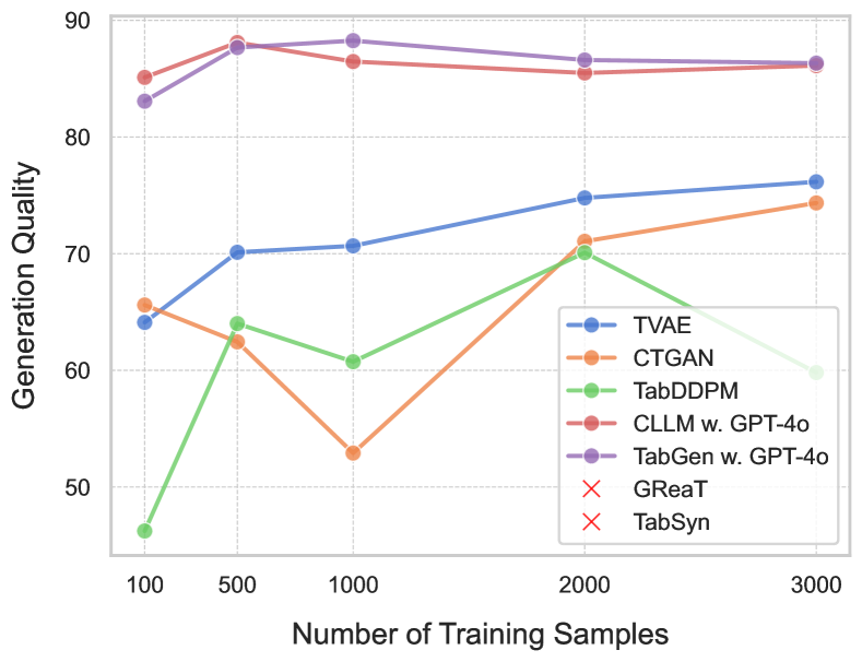
Figure 3: Quality comparison under data-scarcity. TabGen-ICL and CLLM achieves the highest quality score under the few-shot setting. TabSyn and GReaT fail to generate meaningful data.

5.4 TabGen-ICL does not copy training data

In Figure 4, we illustrate the distributions of the L2 distances between the synthetic data and both the training and holdout datasets for CLLM, GReaT, REaLTabFormer (RTF), and TabGen-ICL. Notably, TabGen-ICL exhibits nearly identical distributions for the training and holdout sets, suggesting it is less prone to copying the training data. In contrast, CLLM and GReaT show more disparate distributions, indicating a higher likelihood of relying on the training data.

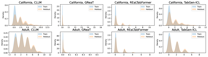
Figure 4: Privacy comparison: Distributions of the DCR scores between the synthetic dataset and the training/holdout datasets. TabGen-ICL and Curated-LLM (CLLM) are both employed with GPT-4o-mini.

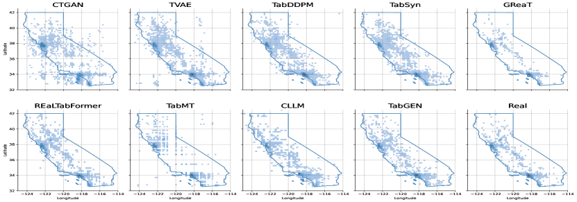
Figure 5: Visual comparison: 2D scatter plot of Longitude and Latitude attributes of California dataset. Real represents the original training datasets. All sets are downsampled to 3000 rows for better visualization. TabGen-ICL generates spatially coherent synthetic data that closely matches the distribution of the original dataset.

5.5 Ablation Study

Effect of $d$.

We examine the effect of the distribution distance metric $d$ used for quantifying residual in Equation 2. We test TabGen-ICL (w. GPT-4o-mini) with only KSD or JSD metric and compare it with our alternating strategy (KSD+JSD) on the California dataset. As shown in Table 3, the alternating strategy achieves the best performance.

$d$	KSD	JSD	KSD+JSD
Marg.	$92.43$$\pm 0.005$	90.72$\pm 0.009$	$92.48$$\pm 0.008$
Corr.	$88.41$$\pm 0.022$	90.67$\pm 0.021$	$91.24$$\pm 0.016$

Table 3: Ablation study for $d$.

Effect of Large Language Models.

In this section, we investigate the impact of large language model (LLM) capabilities on TabGen-ICL’s performance. We evaluate TabGen-ICL using LLMs of varying parameter sizes, including Gemini-1.5-Flash, Gemini-1.5-Pro (Team et al., 2023), Claude-3-Haiku, Claude-3-Sonnet (cla, ), LLaMA-3.1 8B, LLaMA-3.1 405B (Dubey et al., 2024), and Qwen2 (Yang et al., 2024). We assess the marginal metric on the California dataset, with results presented in Table 4. Our findings reveal a correlation between LLM capacity and synthetic data generation quality. As the LLMs’ capacity increases, the quality of generated synthetic data improves. We hypothesize that this improvement stems from larger models’ enhanced ability to capture and reproduce complex patterns within the data, resulting in more realistic synthetic outputs. This relationship underscores the importance of model capacity in generating high-quality synthetic data.

Model	Quality$\uparrow(\%)$	Rank
GPT-4o-mini	$91.86$$\pm 0.008$	3
GPT-4o	$94.69$$\pm 0.006$	1
Gemini-1.5-Flash	$89.96$$\pm 0.017$	4
Gemini-1.5-Pro	$92.21$$\pm 0.033$	2
Claude-3-Haiku	$89.17$$\pm 0.031$	5
Claude-3-Sonnet	$88.97$$\pm 0.068$	6

Table 4: Effect of large language models on the performance of TabGen-ICL.

6 Conclusion

This work proposes TabGen-ICL, an ICL framework for tabular data generation with LLMs. It steer the LLM’s prior distribution towards real data distribution by iteratively retrieving the most under-represented regions. Extensive experiments validate the effectiveness of our approach, demonstrating its potential to enhance LLM-based synthetic data generation across various domains.

7 Limitations

TabGen-ICL relies on a simple heuristic search algorithm to compute residual samples, under which the optimality is not guaranteed. In future, we will explore more principled approaches to compute residuals.

Appendix A Appendix

A.1 Prompts used for generating tabular data

This prompt template is used in Section 4 to generate realistic data that follows the same distribution as the given real data.

⬇

1You are a synthetic data generator tasked with creating new tabular data samples that closely mirror the distribution and characteristics of the original dataset.

2

3# Instruction

41. Analyze the provided real samples carefully.

52. Generate synthetic data that maintains the statistical properties of the real data.

63. Ensure all attributes cover their full expected ranges, including less common or extreme values.

74. Maintain the relationships and correlations between different attributes.

85. Preserve the overall distribution of the real data while introducing realistic variations.

9

10# Key points to consider

11- Replicate the data types of each column (e.g., numerical, categorical).

12- Match the range and distribution of numerical attributes.

13- Maintain the frequency distribution of categorical attributes.

14- Reflect any patterns or trends present in the original data.

15- Introduce realistic variability to avoid exact duplication.

16

17# Real samples

18{data}

19

20# Output format:

21Please present the generated data in a JSON format, structured as a list of objects, where each object represents a single data point with all attributes.

A.2 Dummy Prompt

The following prompt only contains the column names, but not any actual data in it. It is used to produce the results in Fig.1 (a).

⬇

1You are a synthetic data generator tasked with creating new tabular data samples that closely mirror the distribution and characteristics of the original dataset.

2Generate 50 samples of synthetic data.

3

4Each sample should include the following attributes:

5{attributes_list}

6

7Make sure that the numbers make sense for each attribute.

8

9Output Format:

10Present the generated data in a JSON format, structured as a list of objects, where each object represents a single data point with all attributes.

A.3 JSON Schema

The following code define the JSON data class for the structured output function of GPT-4o and GPT-4o-mini.

⬇

1def create_json_model(df: pd.DataFrame, dataname=None) -> BaseModel:

2 fields = {}

3

4 for column in df.columns:

5 if df[column].dtype == ’object’:

6 fields[column] = (str, ...)

7 elif df[column].dtype == ’int64’:

8 fields[column] = (int, ...)

9 elif df[column].dtype == ’float64’:

10 fields[column] = (float, ...)

11 elif df[column].dtype == ’bool’:

12 fields[column] = (bool, ...)

13 else:

14 raise TypeError(f"Unexpected dtype for column {column}: {df[column].dtype}")

15

16 JSONModel = create_model(dataname, **fields)

17

18 class JSONListModel(BaseModel):

19 JSON: List[JSONModel]

20

21 return JSONListModel

A.4 Heuristic for computing residual

In this section, we provide the pseudo-code of our heuristic strategy for computing the residual.

Algorithm 1 Compute residual

1:current dataset $X$, target dataset $Y$, distribution distance $d$.

2:Randomly select a column index $j$

3:if column $j$ is categorical then

4:  Let $C_{j}$ be the number of categories in column $j$

5:  Group samples in $Y$ into $C_{j}$ number of subsets based on its category on column $j$, denote the set of subsets by $(Y_{j}^{i})_{i=1}^{C_{j}}$

6:else

7:  Quantize column $i$ into 50 bins

8:  $C_{j}\leftarrow$ 50

9:  Group samples in $Y$ into $C_{j}$ number of subsets based on its bin index on column $j$, denote the set of subsets by $(Y_{j}^{i})_{i=1}^{C_{j}}$

10:end if

11:for $i=1$ to $C_{j}$ do

12:  Compute distance between $Y_{j}^{i}\cup X$ and $Y$: $d_{i}=d(Y_{j}^{i}\cup X,Y)$

13:end for

14:return subset $Y_{j}^{i}$ that attains the minimal distance.

A.5 Datasets

We use five real-world datasets of varying scales, and all of them are available at Kaggle or the UCI Machine Learning repository. We consider five datasets containing both numerical and catergorical attributes: California, Magic, Adult, Default, Shoppers. The statistics of these datasets are presented in Table 5.

Table 5: Statistics of datasets. # Num stands for the number of numerical columns, and # Cat stands for the number of categorical columns.

Dataset	# Rows	# Num	# Cat	# Train	# Test
California Housing	$20,640$	$9$	1	$18,390$	$2,250$
Magic Gamma Telescope	$19,021$	$10$	1	$17,118$	$1,903$
Adult Income	$32,561$	$6$	$8$	$22,792$	$9,769$
Default of Credit Card Clients	$30,000$	$14$	$10$	$27,000$	$3,000$
Online Shoppers Purchase	$12,330$	$10$	$7$	$11,098$	$1,232$

A.6 Evaluation Metrics

Fidelity

To evaluate if the generated data can faithfully recover the ground-truth data distribution, we employ the following metrics: 1) Marginal distribution: The Marginal metric evaluates if each column’s marginal distribution is faithfully recovered by the synthetic data. We use Kolmogorov-Sirnov Test for continuous data and Total Variation Distance for discrete data. 2) Pair-wise column correlation: This metric evaluates if the correlation between every two columns in the real data is captured by the synthetic data. We compute the Pearson Correlation between all pairs of columns then take average. In addition, we present joint density plots for the Longitude and Latitude features in the California Housing data set in Figure 5. 3) Classifier Two Sample Test (C2ST): This metric evaluates how difficult it is to distinguish real data from synthetic data. Specifically, we create an augmented table that has all the rows of real data and all the rows of synthetic data. Add an extra column to keep track of whether each original row is real or synthetic. Then we train a Logistic Regression classifier to distinguish real and synthetic rows. 4) Precision and Recall: Precision measures the quality of generated samples. High precision means the generated samples are realistic and similar to the true data distribution. Recall measures how much of the true data distribution is covered by the generated distribution. High recall means the model captures most modes/variations present in the true data. 5) Jensen-Shannon Divergence (JSD): This metric evaluates the Jensen-Shannon divergence (Nielsen, 2019) between the distributions of real data and synthetic data.

Utility

We evaluate the utility of the generated data by assessing their performance in Machine Learning Efficiency (MLE). Following the previous works Zhang et al. (2024), we first split a real table into a real training and a real testing set. The generative models are trained on the real training set, from which a synthetic set of equivalent size is sampled. This synthetic data is then used to train a classification/regression model (XGBoost Classifier and XGBoost Regressor (Chen and Guestrin, 2016)), which will be evaluated using the real testing set. The performance of MLE is measured by the AUC score for classification tasks and RMSE for regression tasks.

Privacy

A high-quality synthetic dataset should accurately reflect the underlying distribution of the original data, rather than merely replicating it. To assess this, we employ the Distance to Closest Record (DCR) metric. We begin by splitting the real data into two equal parts: a training set and a holdout set. Using the training set, we generate a synthetic dataset. We then measure the distances between each synthetic data point and its nearest neighbor in both the training and holdout sets. In theory, if both sets are drawn from the same distribution, and if the synthetic data effectively captures this distribution, we should observe an equal proportion (around 50$\%$) of synthetic samples closer to each set. However, if the synthetic data simply copies the training set, a significantly higher percentage would be closer to the training set, well exceeding the expected $50\%$.

A.7 Scalability of TabGen-ICL

To evaluate the scalability of TabGen-ICL, we compare TabGen-ICL with CLLM on a large-scale dataset: Covertype dataset. This dataset consists of 581,012 instances and 54 features. TabGen-ICL and CLLM use iterative in-context learning to generate samples, thus the running time of these two methods are agnostic to the size of the training dataset, making them scalable to large datasets. In the following table, we compare TabGen-ICL with CLLM, employed with both GPT-4o mini and GPT-4o.

Table 6: Performance Comparison on the Covertype Dataset. For all the metrics except AUC, we scale the metrics to a base of $10^{-2}$, and reverse it so that lower values indicate better performance. For AUC, the higher the better.

Model	Marginal $\downarrow$	Corr $\downarrow$	C2ST $\downarrow$	Precision $\downarrow$	Recall $\downarrow$	JSD $\downarrow$	AUC $\uparrow$
CLLM w. GPT-4o	3.28	10.70	55.67	32.32	1.95	0.6078	0.8822
TabGEN w. GPT-4o	2.83	11.10	49.91	24.03	1.27	0.5109	0.9070
Improvement (%)	$\bf{{\color[rgb]{0.8,0.25,0.1}13.72\%}}$	-	$\bf{{\color[rgb]{0.8,0.25,0.1}10.34\%}}$	$\bf{{\color[rgb]{0.8,0.25,0.1}25.62\%}}$	$\bf{{\color[rgb]{0.8,0.25,0.1}34.87\%}}$	$\bf{{\color[rgb]{0.8,0.25,0.1}15.94\%}}$	$\bf{{\color[rgb]{0.8,0.25,0.1}2.81\%}}$
CLLM w. GPT-4o mini	5.35	13.70	0.7796	0.3225	0.0591	0.8743	0.7113
TabGEN w. GPT-4o mini	5.09	12.62	0.7554	0.2876	0.0436	0.9353	0.8311
Improvement (%)	$\bf{{\color[rgb]{0.8,0.25,0.1}4.86\%}}$	$\bf{{\color[rgb]{0.8,0.25,0.1}7.88\%}}$	$\bf{{\color[rgb]{0.8,0.25,0.1}3.11\%}}$	$\bf{{\color[rgb]{0.8,0.25,0.1}10.81\%}}$	$\bf{{\color[rgb]{0.8,0.25,0.1}26.25\%}}$	-	$\bf{{\color[rgb]{0.8,0.25,0.1}16.86\%}}$

The results demonstrate that TabGen-ICL outperforms CLLM on most of the metrics. Notably, the Recall metric again shows the greatest improvement: 34.85% on GPT-4o and 26.25% on GPT-4o mini. This observation is consistent with our original findings in Sec. 5.2. We believe these results strongly support TabGen-ICL’s scalability to larger, more complex datasets.

References

- (1) The claude 3 model family: Opus, sonnet, haiku.
- Assefa et al. (2021) Samuel A. Assefa, Danial Dervovic, Mahmoud Mahfouz, Robert E. Tillman, Prashant Reddy, and Manuela Veloso. 2021. Generating synthetic data in finance: Opportunities, challenges and pitfalls. In Proceedings of the First ACM International Conference on AI in Finance, ICAIF ’20. Association for Computing Machinery.
- Benjelloun et al. (2020) Omar Benjelloun, Shiyu Chen, and Natasha Noy. 2020. Google dataset search by the numbers. In International Semantic Web Conference, pages 667–682. Springer.
- Borisov et al. (2023) Vadim Borisov, Kathrin Sessler, Tobias Leemann, Martin Pawelczyk, and Gjergji Kasneci. 2023. Language models are realistic tabular data generators. In International Conference on Learning Representations.
- Cao et al. (2019) Kaidi Cao, Colin Wei, Adrien Gaidon, Nikos Arechiga, and Tengyu Ma. 2019. Learning imbalanced datasets with label-distribution-aware margin loss. Advances in neural information processing systems, 32.
- Chen and Guestrin (2016) Tianqi Chen and Carlos Guestrin. 2016. Xgboost: A scalable tree boosting system. In ACM SIGKDD Conference on Knowledge Discovery and Data Mining, pages 785–794.
- Dubey et al. (2024) Abhimanyu Dubey, Abhinav Jauhri, Abhinav Pandey, Abhishek Kadian, Ahmad Al-Dahle, Aiesha Letman, Akhil Mathur, Alan Schelten, Amy Yang, Angela Fan, et al. 2024. The llama 3 herd of models. arXiv preprint arXiv:2407.21783.
- Even et al. (2007) Adir Even, Ganesan Shankaranarayanan, and Paul D Berger. 2007. Economics-driven data management: An application to the design of tabular data sets. IEEE Transactions on Knowledge and Data Engineering, 19(6):818–831.
- Gao et al. (2023) Yunfan Gao, Yun Xiong, Xinyu Gao, Kangxiang Jia, Jinliu Pan, Yuxi Bi, Yi Dai, Jiawei Sun, and Haofen Wang. 2023. Retrieval-augmented generation for large language models: A survey. arXiv preprint arXiv:2312.10997.
- Gascón et al. (2016) Adrià Gascón, Phillipp Schoppmann, Borja Balle, Mariana Raykova, Jack Doerner, Samee Zahur, and David Evans. 2016. Privacy-preserving distributed linear regression on high-dimensional data. Cryptology ePrint Archive.
- Goodfellow et al. (2014) Ian J Goodfellow, Jean Pouget-Abadie, Mehdi Mirza, Bing Xu, David Warde-Farley, Sherjil Ozair, Aaron Courville, and Yoshua Bengio. 2014. Generative adversarial nets. In Advances in Neural Information Processing Systems, pages 2672–2680.
- Gulati and Roysdon (2023) Manbir S Gulati and Paul F Roysdon. 2023. Tabmt: generating tabular data with masked transformers. In Advances in Neural Information Processing Systems, pages 46245–46254.
- Hernandez et al. (2022) Mikel Hernandez, Gorka Epelde, Ane Alberdi, Rodrigo Cilla, and Debbie Rankin. 2022. Synthetic data generation for tabular health records: A systematic review. Neurocomputing, 493:28–45.
- Kim et al. (2023) Jayoung Kim, Chaejeong Lee, and Noseong Park. 2023. Stasy: Score-based tabular data synthesis. In International Conference on Learning Representations.
- Kingma and Welling (2013) Diederik P Kingma and Max Welling. 2013. Auto-encoding variational bayes. arXiv preprint arXiv:1312.6114.
- Kotelnikov et al. (2023) Akim Kotelnikov, Dmitry Baranchuk, Ivan Rubachev, and Artem Babenko. 2023. Tabddpm: Modelling tabular data with diffusion models. In International Conference on Machine Learning, pages 17564–17579. PMLR.
- Lee et al. (2023) Chaejeong Lee, Jayoung Kim, and Noseong Park. 2023. Codi: Co-evolving contrastive diffusion models for mixed-type tabular synthesis. In International Conference on Machine Learning, pages 18940–18956. PMLR.
- Lin and Tsai (2020) Wei-Chao Lin and Chih-Fong Tsai. 2020. Missing value imputation: a review and analysis of the literature (2006–2017). Artificial Intelligence Review, 53:1487–1509.
- Liu et al. (2024) Michael Xieyang Liu, Frederick Liu, Alexander J Fiannaca, Terry Koo, Lucas Dixon, Michael Terry, and Carrie J Cai. 2024. " we need structured output": Towards user-centered constraints on large language model output. In Extended Abstracts of the CHI Conference on Human Factors in Computing Systems, pages 1–9.
- Liu et al. (2023) Tennison Liu, Zhaozhi Qian, Jeroen Berrevoets, and Mihaela van der Schaar. 2023. Goggle: Generative modelling for tabular data by learning relational structure. In International Conference on Learning Representations.
- Nielsen (2019) Frank Nielsen. 2019. On the jensen–shannon symmetrization of distances relying on abstract means. Entropy, 21(5):485.
- Seedat et al. (2024) Nabeel Seedat, Nicolas Huynh, Boris van Breugel, and Mihaela van der Schaar. 2024. Curated LLM: Synergy of LLMs and data curation for tabular augmentation in low-data regimes. In Forty-first International Conference on Machine Learning.
- Singha et al. (2023) Ananya Singha, José Cambronero, Sumit Gulwani, Vu Le, and Chris Parnin. 2023. Tabular representation, noisy operators, and impacts on table structure understanding tasks in llms. arXiv preprint arXiv:2310.10358.
- Solatorio and Dupriez (2023) Aivin V. Solatorio and Olivier Dupriez. 2023. Realtabformer: Generating realistic relational and tabular data using transformers. arXiv preprint arXiv:2302.02041.
- Sui et al. (2024) Yuan Sui, Mengyu Zhou, Mingjie Zhou, Shi Han, and Dongmei Zhang. 2024. Table meets llm: Can large language models understand structured table data? a benchmark and empirical study. In Proceedings of the 17th ACM International Conference on Web Search and Data Mining, pages 645–654.
- Team et al. (2023) Gemini Team, Rohan Anil, Sebastian Borgeaud, Yonghui Wu, Jean-Baptiste Alayrac, Jiahui Yu, Radu Soricut, Johan Schalkwyk, Andrew M Dai, Anja Hauth, et al. 2023. Gemini: a family of highly capable multimodal models. arXiv preprint arXiv:2312.11805.
- Wang et al. (2024) Yuxin Wang, Duanyu Feng, Yongfu Dai, Zhengyu Chen, Jimin Huang, Sophia Ananiadou, Qianqian Xie, and Hao Wang. 2024. Harmonic: Harnessing llms for tabular data synthesis and privacy protection. ArXiv, abs/2408.02927.
- Xu et al. (2019) Lei Xu, Maria Skoularidou, Alfredo Cuesta-Infante, and Kalyan Veeramachaneni. 2019. Modeling tabular data using conditional gan. In Advances in Neural Information Processing Systems, page 7335–7345.
- Xu et al. (2024a) Shengzhe Xu, Cho-Ting Lee, Mandar Sharma, Raquib Bin Yousuf, Nikhil Muralidhar, and Naren Ramakrishnan. 2024a. Are llms naturally good at synthetic tabular data generation? ArXiv, abs/2406.14541.
- Xu et al. (2024b) Shengzhe Xu, Cho-Ting Lee, Mandar Sharma, Raquib Bin Yousuf, Nikhil Muralidhar, and Naren Ramakrishnan. 2024b. Are llms naturally good at synthetic tabular data generation? arXiv preprint arXiv:2406.14541.
- Yang et al. (2024) An Yang, Baosong Yang, Binyuan Hui, Bo Zheng, Bowen Yu, Chang Zhou, Chengpeng Li, Chengyuan Li, Dayiheng Liu, Fei Huang, et al. 2024. Qwen2 technical report. arXiv preprint arXiv:2407.10671.
- Zhang et al. (2024) Hengrui Zhang, Jiani Zhang, Zhengyuan Shen, Balasubramaniam Srinivasan, Xiao Qin, Christos Faloutsos, Huzefa Rangwala, and George Karypis. 2024. Mixed-type tabular data synthesis with score-based diffusion in latent space. In International Conference on Learning Representations.
- Zhang et al. (2023) Tianping Zhang, Shaowen Wang, Shuicheng Yan, Jian Li, and Qian Liu. 2023. Generative table pre-training empowers models for tabular prediction. arXiv preprint arXiv:2305.09696.
- Zhao et al. (2023) Zilong Zhao, Robert Birke, and Lydia Chen. 2023. Tabula: Harnessing language models for tabular data synthesis. arXiv preprint arXiv:2310.12746.
- Zheng and Charoenphakdee (2022) Shuhan Zheng and Nontawat Charoenphakdee. 2022. Diffusion models for missing value imputation in tabular data. arXiv preprint arXiv:2210.17128.