Preserving Simultaneity and Chronology for Sensing in Wireless Perceptive Networks

Abstract

We address the challenge of preserving the simultaneity and chronology of sensing events in multi-sensory systems with wireless links. The network uses temporal windows of integration (TWIs), borrowed multi-sensory perception, to preserve the temporal structure of the sensing data at the application side. We introduce a composite latency model for propagation, sensing, and communication that leads to the derivation of the probability of simultaneity violation. This is used to select the TWI duration aiming to achieve the desired degrees of chronological preservation, while maintaining the throughput of events. The letter provides important insights and analytical tools about the TWI impact on the event registration.

I Introduction

THE evolution towards perceptive mobile networks [1], together with edge-computing and AI-native technologies, is creating a platform of unprecedented tools to monitor and control cyber-physical systems. Base stations (BSs) are expected to get multimodal inputs from sensors and Internet of Things (IoT) devices, supporting complex learning/inference tasks and capturing associations between data modalities for insights into physical processes [2]. It has been shown that multimodal processing can improve the performance of target tracking systems [3]. However, multimodal sensor fusion is prone to the reception of out-of-order measurements due to random delays induced by, e.g., communication. In estimation and inference tasks, outdated measurements received out-of-order can be leveraged by applying retrodiction followed by an update step [4]. However, such a strategy is not suitable in decision tasks, as different execution paths may be taken depending on the observations. Resilient task completion requires preservation of event chronology, ensuring that all measurements will be processed in the order they were originally generated.

In distributed systems, message ordering protocols based on logical clocks can preserve the correct chronology of sensor updates, ensuring delivery to the application in their original order [5]. Nonetheless, such protocols introduce significant overhead for sharing vector clocks, while they cannot handle physical events before they are converted to the digital domain by, e.g., sensing [6]. Alternatively, when the delay to receive a sensor update has a known upper bound [7], it can be used to set a deadline to start processing only after receiving all updates. Similarly, but based on mechanisms that enable the human multi-sensory perception, the temporal window of integration (TWI) framework [6] proposes the establishment of timing constraints to process events, guaranteeing their correct temporal ordering and tracking the possible causal relations between them. A related work [8] considers out-of-order arrivals from the Age of Information perspective.

Inspired by the TWI framework, we address the problem of event chronology when receiving status updates from wireless sensors that observe the same physical process, delivering to an application hosted at a BS. We extend [6] by developing a model that covers the propagation of physical signals generated by the monitored process, the computation delay involved in the sensing task, and the communication delay to convey the updates to the BS. By applying this model, we derive the probability of simultaneity violation (PSV) in a scenario where event-driven updates related to a physical process must be delivered concurrently to the application. Then, we design the TWI duration to provide statistical guarantees that the delivery to the application of status updates generated by the same physical event will attain a target PSV. The analysis is supplemented by numerical results that reveal interesting tendencies about the impact of the choice of TWI on the performance in terms of simultaneity preservation.

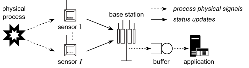
Figure 1: System to monitor a physical process from event-driven status updates produced by wireless sensors.

II System Model

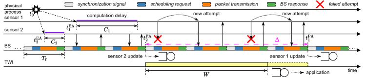
Figure 2: Timing diagram illustrating a physical process event, the generation and transmission of status updates related to that event by two sensors, and the delivery of the updates to the application based on the TWI framework. In this scenario, sensor 1’s update arrived later than sensor 2’s due to the longer propagation and computation delays, and the delay resulting from the failed SR and packet transmission attempt. In this example, the TWI design is inadequate for the simultaneous delivery of the updates: the TWI lasts for three frames, while the update arrival times are separated by four frames.

We consider the scenario in Fig. 1, in which an application hosted at the BS monitors a physical process based on event-driven status updates sent by $I\in\mathbb{N}_{+}$ wireless sensors. When the physical process generates an event, the sensors produce and transmit updates regarding it. All the updates resulting from the same physical event need to be considered simultaneous from the application perspective. Therefore, the BS must ensure that all received updates will be delivered concurrently to the application. To do so, the BS stores the updates in a buffer, delivering them and cleaning the buffer under two situations: 1) when all $I$ updates have been successfully received and stored, or 2) when $W>0$ seconds have passed after the reception and storage of the first update. Hence, $W$ denotes the maximum time window at which the application will perceive status updates as simultaneous and, accordingly, is the duration of the application TWI [6].

Definition 1 (Simultaneity violation)

A simultaneity violation event occurs at the application when updates related to the same physical event are delivered in different TWIs. We refer to its probability as the PSV.

To design the TWI duration $W$, we aim to link it to the PSV; this is done by evaluating the packet delay variation (PDV).

Definition 2 (Packet delay variation)

The PDV is defined as the time interval between the reception at the BS of the first (fastest) and last (slowest) status updates.

The investigation is carried out under the sensing and communication processes depicted in Fig. 2 and detailed below.

II-1 Sensing Process

The monitored process generates events in the form of physical signals (e.g., acoustic, seismic, optical), propagating toward sensors at the speed $v>0$. For simplicity, in this study we consider that the sensors observe only one type of physical signal. We assume the time interval between two consecutive events to be much larger than the application’s TWI, such that new events do not occur while the BS receives status updates produced by an event. The time an event occurred is denoted by $t_{0}\geq 0$. Sensors are uniformly distributed over a circular region with radius $D_{\max}>0$, centered at the position of the monitored process. The probability density function (PDF) of the distance from the $i-$th sensor to the physical process is

$$f_{D}(d)=\frac{2d}{D_{\max}^{2}},\,\,d\in[0,D_{\max}].$$ (1)

Since the physical signals generated by the process events travel at a limited speed, depending on the distance $D_{i}$, the propagation delay cannot be neglected. Accordingly, we define the event action time of sensor $i$ as the time at which the physical signals arrive such a sensor, i.e.,

$$t_{i}^{\text{EA}}=t_{0}+\frac{D_{i}}{v}.$$ (2)

The sensors produce event-driven status updates based on observations of the physical signals, following a change-aware sampling and communication policy [9]. A status update comprises a data packet containing $b\in\mathbb{N}_{+}$ bits. To produce a single update, a sensor induces a computation delay $C_{i}\sim\mathcal{U}(C_{\min},C_{\max})$, where $0<C_{\min}<C_{\max}$ are the best- and worst-case computation delays, respectively. This stochastic model reflects the device heterogeneity in larger sensor populations, where irregular computation delays can be due to, e.g., different hardware platforms.

II-2 Communication Process

The sensors send the status updates through wireless transmissions dynamically scheduled by the BS. We consider a narrowband frame-based communication process of bandwidth $B>0$ and frame duration $T_{\text{f}}>0$ as in Fig. 2. Each frame has downlink (DL) and uplink (UL) sub-frames: synchronization signal (SS) (DL), scheduling request (SR) (UL), packet transmission (UL), and BS response (DL). We assume a block-fading channel with channel coefficient $h_{i}\sim\mathcal{CN}(0,\beta_{i})$ between the BS and sensor $i$, where $\beta_{i}$ is the large-scale fading, known for all $I$ sensors.

Transmissions are scheduled upon random access requests made individually by the sensors after producing their status updates. To send a request, sensor $i$ first listens to a SS to acquire frame synchronization; then, during the SR subframe, it transmits the preamble $\bm{s}_{i}\in\mathbb{C}^{S}$ such that $S\geq I$ and $\|\bm{s}_{i}\|=1$, with transmit power $P_{i}>0$. Such a preamble defines a unique identifier for each sensor and is taken from a set of mutually orthogonal sequences, i.e., $\bm{s}_{i}^{\htransp}\bm{s}_{j}=0,\leavevmode\nobreak\ \forall i\neq j$. Therefore, no preamble collision occurs if multiple sensors send simultaneous SRs. Let $\mathcal{I}$ denote the indices of the sensors that sent an SR during a specific frame and $\bm{n}\sim\mathcal{CN}(\bm{0},N_{0}B\bm{I})$ the thermal noise at the BS receiver, with $N_{0}>0$ being the noise spectral density. The UL received signal at the BS containing the SR preambles is denoted as:

$$\bm{y}=\sum_{i\in\mathcal{I}}h_{i}\sqrt{P_{i}}\bm{s}_{i}+\bm{n}.$$ (3)

While no collision can happen in our setting, the BS needs to detect transmitted scheduling preambles to decode them. We assume the BS employs a maximum likelihood detection process on the normalized received signal correlated with the preamble, i.e., $\hat{y}_{i}=\bm{s}_{i}^{\htransp}\bm{y}/\sqrt{P_{i}N_{0}B}$. Using standard detection theory [10], this processing yields the optimal threshold $\eta_{i}=(1+\gamma_{i}^{-1})\ln(1+\gamma_{i})$, where $\gamma_{i}=P_{i}\beta_{i}/(N_{0}B)$ is the average received signal-to-noise ratio (SNR) at the BS. When the BS detects the preambles transmitted by a generic sensor $i$, i.e., whenever $\hat{y}_{i}\geq\eta_{i}$, for any $i\in\{1,\dots,I\}$, it sends a scheduling grant in the BS response sub-frame intended for the preamble’s owner. The scheduling grant is assumed orthogonal among users. A scheduling grant allows a sensor to transmit its status update in the next communication frame, within the packet transmission sub-frame. If a sensor that sent an SR does not find a grant intended for it in the BS response, it will make a new attempt in the subsequent frame. Each sensor can send an SR up to $M_{\max}\in\mathbb{N}_{+}$ times, including the first attempt. The number of attempts sent by sensor $i$ is denoted by $m_{i}\leq M_{\max}$ and a packet is dropped when the sensor does not receive a scheduling grant after the $M_{\max}$-th attempt.

After receiving a scheduling grant in a frame, the sensor uses the packet transmission opportunity of the next frame to send its status update. If more than one sensor got a scheduling grant in a frame, then the BS uses round-robin scheduling to accommodate all packet transmissions. Let $0<T_{\text{p}}<T_{\text{f}}$ denote the time interval of the packet transmission opportunity in a frame. We have assumed a quasi-static fading channel which has zero dispersion [11]; thus, finite blocklength effects are negligible and the outage probability accurately captures the error performance. The transmission of sensor $i$ is in outage if the instantaneous SNR measured at the BS is less than $\gamma_{\text{TH}}=2^{b/(T_{\text{p}}B)}-1$. Therefore, the outage probability is:

$$\epsilon_{i}=\Pr\left\{\frac{P_{i}|h_{i}|^{2}}{N_{0}B}<\gamma_{\text{TH}}\right\}=1-\exp\left\{-\frac{\gamma_{\text{TH}}}{\gamma_{i}}\right\},$$ (4)

given that $|h_{i}|^{2}\sim\mathrm{Exp}(1/\beta_{i})$. When a transmission does not incur an outage, the BS successfully receives the packet and sends an acknowledgment to the sensor in the BS response of the same frame. Otherwise, if an outage occurs, the BS provide a new scheduling grant for the transmitting sensor in the BS response sub-frame; the sensor can attempt the packet transmission during the subsequent frame. A scheduled sensor can make up to $N_{\max}\in\mathbb{N}_{+}$ transmission attempts before dropping its packet, while we denote the number of transmission attempts made by sensor $i$ by $n_{i}\leq N_{\max}$. $N_{\max}$ is not necessarily equal to $M_{\max}$.

From the system model, one can perceive that the propagation of the physical signals generated by the monitored process, the computation by the sensors, and the communication with the BS introduce random delays in the reception of status updates produced by an event. To design the application TWI duration, we need to understand how these delays affect the arrival times of the first and last received status updates at the BS, as investigated in the following section.

III TWI Design Based on the Distribution of the Packet Delay Variation

In this section, we first develop statistical models for the sensors’ packet arrival time at the BS and the PDV between the first and last received status updates. Then, we design the application TWI duration based on the characteristics of the physical, sensing, and communication processes.

We analyzed three timing components: 1) the physical event action time, 2) the sensor computation delay, and 3) the communication delay. All results are conditioned to the event time $t_{0}$ and propagation velocity $v$, the average SNRs $\{\gamma_{i}\}_{i=1}^{I}$, and the communication parameters $T_{\text{f}}$, $M_{\max}$, and $N_{\max}$.

When conditioned to $t_{0}$ and $v$, the PDF of $t_{i}^{\text{EA}}$ depends only on the PDF of $D_{i}$. Hence, from eq. (1), the PDF of $t_{i}^{\text{EA}}$ is

$$t_{i}^{\text{EA}}\sim\frac{2v^{2}(t-t_{0})}{D_{\max}^{2}},\,\,t\in\left[t_{0},t_{0}+\frac{D_{\max}}{v}\right].$$ (5)

After detecting the physical signals generated by the monitored process, sensor $i$ takes the $C_{i}\sim f_{C}$ seconds to perform computations and produce its status update. According to Section II, $f_{C}$ is a uniform PDF; such a model is sufficient to evaluate the delay induced by the computation.

To analyze the delay induced by communication, we assume no packet drop occurs, i.e., $1\leq m_{i}\leq M_{\text{max}}$ and $1\leq n_{i}\leq N_{\text{max}}$, and evaluate the probability mass function (PMF) of the time needed for SRs and packet transmission. With the scheduling procedure described in Section II, the probability of the BS failing in detecting the SR of sensor $i$ is

$$\zeta_{i}=1-(1+\gamma_{i})^{-\frac{1}{\gamma_{i}}}.$$ (6)

Due to the independent block-fading channel assumption, $\zeta_{i}$ is a sufficient statistic to model $m_{i}$, which follows a geometric distribution, i.e., $m_{i}\sim\text{Geo}(1-\zeta_{i})$. Therefore, the SRs induce a delay of $T_{i}^{\text{SR}}=m_{i}T_{\text{f}}$, distributed as

$$T_{i}^{\text{SR}} \sim\Pr\{T_{i}^{\text{SR}}=mT_{\text{f}}|1\leq m\leq M_{\max}\}$$ (7)

$$=\sum_{j=1}^{M_{\max}}\frac{\zeta_{i}^{m-1}(1-\zeta_{i})\delta(j-m)}{1-\zeta_{i}^{K_{\max}}},\,\,\forall m\in\{1,\dots,M_{\max}\}.$$

A similar analysis can be applied to the packet transmission. From eq. (4), we have $n_{i}\sim\text{Geo}(1-\epsilon_{i})$. Hence, the delay induced by the packet transmission is $T_{i}^{\text{PT}}=n_{i}T_{\text{f}}$, such that

$$T_{i}^{\text{PT}} \sim\Pr\{T_{i}^{\text{PT}}=nT_{\text{f}}|1\leq n\leq N_{\max}\}$$ (8)

$$=\sum_{j=1}^{N_{\max}}\frac{\epsilon_{i}^{n-1}(1-\epsilon_{i})\delta(j-n)}{1-\epsilon_{i}^{N_{\max}}},\,\,\forall n\in\{1,\dots,N_{\max}\}.$$

The three timing components can be combined to obtain the packet arrival time. Taking into account that sensors acquire frame synchronization through SS and considering that the first frame starts at time $t=0$, the packet arrival time is

$$t_{i}^{\text{PA}}=\left\lceil\frac{t_{i}^{\text{EA}}+C_{i}}{T_{\text{f}}}\right\rceil T_{\text{f}}+T_{i}^{\text{SR}}+T_{i}^{\text{PT}},$$ (9)

where the ceiling function ensures the time is aligned with the start of the first available frame after the computation process. We remark that $t_{i}^{\text{PA}}=\infty$ if a packet drop event occurs for sensor $i$. Formally, this event is $\mathcal{L}_{i}=\{m_{i}>M_{\max}\cup n_{i}>N_{\max}\}$, having a packet drop rate given by the probability

$$\rho_{i}=\Pr\{\mathcal{L}_{i}\}=\zeta_{i}^{M_{\max}}+\epsilon_{i}^{N_{\max}}-\zeta_{i}^{M_{\max}}\epsilon_{i}^{N_{\max}},$$ (10)

According to Definition 2, the PDV is obtained from the difference between the arrival times of the last and the first packet received by the BS. Therefore, the PDV is

$$\Delta=\max_{i\in\mathcal{I}^{\prime}}\{t_{i}^{\text{PA}}\}-\min_{i\in\mathcal{I}^{\prime}}\{t_{i}^{\text{PA}}\},$$ (11)

where $\mathcal{I}^{\prime}\subseteq\{1,\dots,I\}$ is the subset of sensors not experiencing a packet drop event. The distribution of the PDV for a generic population of $I$ sensors can be derived using order statistics. In this paper, however, we aim to provide a simpler analytical interpretation of system behavior. To achieve this, we focus on a system with $I=2$, reducing the complexity of the PDV analysis. Even with $I=2$, deriving a closed-form expression for $\Delta$ remains challenging due to the mix of continuous and discrete random variables and the ceiling function at eq. (9). To facilitate a tractable design of the TWI, we propose two approximations for the statistical distribution of $\Delta$: one that applies when the computation delay primarily governs the PDV and another suited to cases where event action time is the dominant factor.

To approximate the PDV distribution, we look in the case with $I=2$ sensors. The PDV of eq. (11) can be rewritten as

$$\Delta=|t_{1}^{\text{PA}}-t_{2}^{\text{PA}}|.$$ (12)

From here on, the PDV $\Delta$ refers to this particular case.

The first approximation addresses the case where the computation delay governs the PDV. This happens when $C_{i}$ can assume values significantly higher than $t_{i}^{\text{EA}}$ and $T_{i}^{\text{SR}}+T_{i}^{\text{PT}}$. Thus, the PDV is approximated by

$$\Delta\approx\Delta_{\text{Comp.}}=|C_{1}-C_{2}|,$$ (13)

whose PDF and cumulative distribution function (CDF) are given in Lemma 1.

Lemma 1

The PDF of $\Delta_{\text{Comp.}}$ is

$$\textstyle f_{\Delta_{\text{Comp.}}}(t)=\frac{2(C_{\max}-C_{\min}-t)}{(C_{\max}-C_{\min})^{2}},\,\,t\in[0,C_{\max}-C_{\min}],$$ (14)

while the CDF of $\Delta_{\text{Comp.}}$ is given by

$$F_{\Delta_{\text{Comp.}}}(t)=\begin{cases}\frac{2(C_{\max}-C_{\min})t-t^{2}}{(C_{\max}-C_{\min})^{2}},&t\in[0,C_{\max}-C_{\min}],\\ 1,&t>C_{\max}-C_{\min}.\end{cases}$$ (15)

Proof:

See Appendix. ∎

The second approximation covers the case where the propagation delay of the event physical signals is predominant at the PDV. This might be the case for big $D_{\max}$ or small $v$. Accordingly, the PDV can be approximated by

$$\Delta\approx\Delta_{\text{Prop.}}=|t_{1}^{\text{EA}}-t_{2}^{\text{EA}}|=\left|\frac{D_{1}}{v}-\frac{D_{2}}{v}\right|,$$ (16)

whose PDF and CDF are given by Lemma 2.

Lemma 2

The PDF of $\Delta_{\text{Prop.}}$ is

$$\textstyle f_{\Delta_{\text{Prop.}}}(t)=\frac{2v^{4}}{3D_{\max}^{4}}\left(2t^{3}\hskip-2.84526pt-\hskip-2.84526pt\frac{6D_{\max}^{2}}{v^{2}}t\hskip-2.84526pt+\hskip-2.84526pt\frac{4D_{\max}^{3}}{v^{3}}\right),\,\,t\in\left[0,\frac{D_{\max}}{v}\right],$$ (17)

and the CDF of $\Delta_{\text{Prop.}}$ is given by

$$F_{\Delta_{\text{Prop.}}}(t)\hskip-2.84526pt=\hskip-2.84526pt\begin{cases}\frac{2v^{4}}{3D_{\max}^{4}}\hskip-2.84526pt\left(\frac{1}{2}t^{4}\hskip-2.84526pt-\hskip-2.84526pt\frac{3D_{\max}^{2}}{v^{2}}t^{2}\hskip-2.84526pt+\hskip-2.84526pt\frac{4D_{\max}^{3}}{v^{3}}t\right),&t\in\big{[}0,\frac{D_{\max}}{v}\big{]},\\ 1,&t>\frac{D_{\max}}{v}.\end{cases}$$ (18)

Proof:

See Appendix. ∎

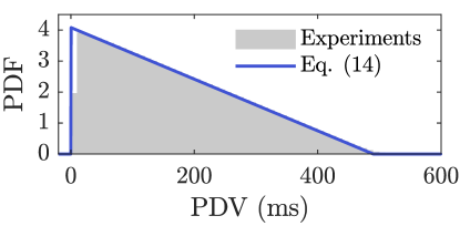
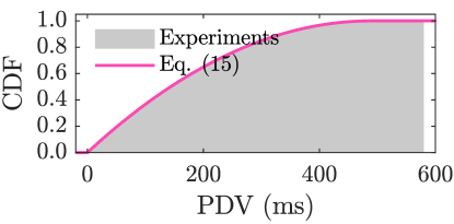
(a) Approximation of eq. (13). $v=3\cdot 10^{8}$ m/s, $\mathcal{C}=(10,500)$.

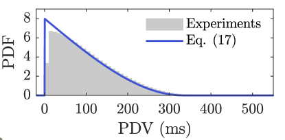
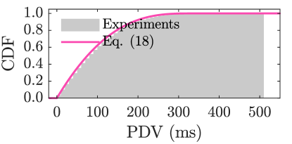
(b) Approximation of eq. (16). $v=300$ m/s, $\mathcal{C}=(10,100)$.

Figure 3: Approximations for the PDF and CDF of the PDV compared with experiments computed from eq. (12). $D_{\max}=100$ m, $T_{\text{f}}=10$ ms, $M_{\max}=N_{\max}=5$, $\gamma_{2}=\gamma_{\text{TH}}=1$, $\mathcal{C}=(C_{\min},C_{\max})$ in ms.

By definition, the CDFs (15) and (18) represent the probability that the PDV is below a given time, which is essential for verifying if status updates reach the BS in time for concurrent delivery toward the application. Based on these and the application requirements, we can determine the optimal TWI for cases where the approximations hold. To show the accuracy of the approximations, Fig. 3 depicts the PDFs and CDFs of Lemmas 1 and 2 along with empirical distributions of the PDV obtained through experiments from eq. (12).

In terms of TWI design, with $I=2$, the simultaneity violation happens if, upon the reception of one packet containing a status update, the packet containing the other is dropped by its sensor or arrives at the BS after the TWI duration. Without loss of generality, assuming that the BS received first from sensor 1, the PSV is

$$\sigma=\Pr\{\mathcal{L}_{2}\cup\Delta>W\}=1-(1-\rho_{2})\Pr\{\Delta<W\},$$ (19)

where $\mathcal{L}_{2}$ and $\rho_{2}$ are the packet drop event and rate for sensor $i=2$, see eq. (10). By replacing the CDF of $\Delta$ with the approximation of eq. (15) in (19), we get the PSV when the computation delay governs the PDV, that is

$$\sigma_{\text{Comp.}}=1-(1-\rho_{2})F_{\Delta_{\text{Comp.}}}(W).$$ (20)

Conversely, by replacing the CDF of $\Delta$ with eq. (18), we get the PSV when the propagation delay governs the PDV, that is

$$\sigma_{\text{Prop.}}=1-(1-\rho_{2})F_{\Delta_{\text{Prop.}}}(W).$$ (21)

By inverting eqs. (20) and (21), we can design the TWI duration satisfying a target PSV.

IV Numerical Results

In this section, we deploy a performance analysis of the system through numerical simulations. We assume the physical process event occurs at $t_{0}=0$ for all results. Moreover, realizations of the random variables are computed by sampling the random distributions defined in Section III.

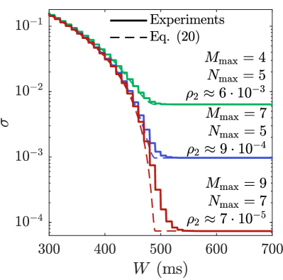
(a) $v=3\cdot 10^{8}$ m/s, $\mathcal{C}=(10,500)$.

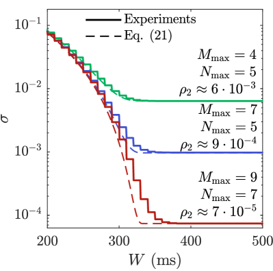
(b) $v=300$ m/s, $\mathcal{C}=(0,10)$.

Figure 4: PSV calculated by the approximations of (a) eq. (20) and (b) eq. (21), and obtained in experiments computed from eq. (19). $D_{\max}=100$ m, $T_{\text{f}}=10$ ms, $\gamma_{2}=4$, $\gamma_{\text{TH}}=1$, $\mathcal{C}=(C_{\min},C_{\max})$ in ms.

The comparison between the analytical and the experimental PSV is depicted in Fig. 4, tested different communication parameters and their relative packet drop rate. Specifically, the probability obtained in the experiments is compared with the approximation of eq. (20) in Fig. 4a and (21) in Fig. 4b. The curves reveal that the approximations accurately model the PSV, making it possible to design $W$ based on a target $\sigma$. Moreover, the PSV is bounded by $\rho_{2}$, meaning that a full optimization of the system must account not only for the TWI duration but also for the communication parameters.

Using the statistical model from Section III, we show how the delivery of status updates affects the application. Here latency is the interval from $t_{0}$ to the delivery of the status updates to the application within the first available TWI. We analyze two cases: 1) when the packet of sensor 2 arrives before the end of the TWI, the updates are concurrently delivered at the time $t_{1}^{\text{PA}}+\Delta$; and, 2) when the sensor 2’s packet is received in a different TWI, the first update is delivered alone at the time $t_{1}^{\text{PA}}+W$. Thus, the latency can be written as $L=t_{1}^{\text{PA}}+\min\{\Delta,W\}-t_{0}$. Fig. 5 shows the values of $L$ obtained with different system parameters. By evaluating multiple setups, we can verify how the physical process and computation parameters affect the definition of $W$ and the induced $L$. One might notice that the average $L$ can be lower than the TWI, as the random delays can make the second update arrive less than $W$ seconds after the first one.

(a) $D_{\max}=100$ m, $v=3\cdot 10^{8}$ m/s, $\mathcal{C}_{k}=(C_{\min},C_{\max})$ in ms.

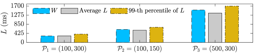
(b) $C_{\min}=0$, $C_{\max}=10$ ms, $\mathcal{P}_{k}=(D_{\max},v)$ in m and m/s.

Figure 5: TWI computed by the approximations of (a) eq. (20) and (b) eq. (21) to achieve $\sigma=10^{-3}$ and resulting latency obtained in different setups. $T_{\text{f}}=10$ ms, $\gamma_{2}=4$, $\gamma_{\text{TH}}=1$, $M_{\max}=9$, $N_{\max}=7$, $\rho_{2}=7\cdot 10^{-5}$.

V Discussion and Conclusions

In this paper, we have addressed the problem of event chronology in the reception of status updates of sensors observing the same physical process. By modeling the random delays involved in the generation and transmission of the updates, we proposed a TWI duration design to attain a target PSV for a two-sensors scenario, validating it through numerical experiments. Potential applications of our findings include the evaluation of the closed-loop latency of control tasks that empower the TWI framework for processing observations acquired in a distributed manner in the chronological order they were generated. Future works will generalize the analysis to scenarios with more than two sensors, capitalizing on the findings for monitoring cyber-physical systems.

To develop the proof of Lemma 1 and 2, we use the CDF method to obtain the PDF of the absolute difference between two random variables. Let us define the random variables $X_{1},X_{2}\sim f_{X}$ and $Y=|X_{1}-X_{2}|\sim f_{Y}$. Thus, we have

$$F_{Y}(y) =\Pr\{|X_{1}-X_{2}|<y\}=\Pr\{-y<X_{1}-X_{2}<y\},$$

$$=\int_{-\infty}^{\infty}\int_{x_{2}-y}^{x_{2}+y}f_{X}(x_{1})\leavevmode\nobreak\ f_{X}(x_{2})\leavevmode\nobreak\ dx_{1}\leavevmode\nobreak\ dx_{2}.$$ (22)

Then, the PDF of $Y$ can be obtained by evaluating the derivative of (22) w.r.t. $y$, obtaining

$$f_{Y}(y)=\int_{-\infty}^{\infty}[f_{X}(x_{2}+y)+f_{X}(x_{2}-y)]\leavevmode\nobreak\ f_{X}(x_{2})\leavevmode\nobreak\ dx_{2}.$$ (23)

In Lemma 1, we have $X_{1}=C_{1}$, $X_{2}=C_{2}$, $Y=\Delta_{\text{Comp.}}$, $f_{X}=\mathcal{U}(C_{\min},C_{\max})$, and $f_{Y}=f_{\Delta_{\text{Comp.}}}$. Accordingly, by substituting these quantities and solving the integral, we obtain $f_{\Delta_{\text{Comp.}}}$ as in (14). Then, by integrating eq. (14) w.r.t. $t$, we obtain $F_{\Delta_{\text{Comp.}}}$ as in (15), completing the proof.

In Lemma 2, $X_{1}=D_{1}/v$, $X_{2}=D_{2}/v$, $Y=\Delta_{\text{Prop.}}$, $f_{X}=f_{D}$ as in (1), and $f_{Y}=f_{\Delta_{\text{Prop.}}}$. By substituting these quantities in the integral, we obtain $f_{\Delta_{\text{Prop.}}}$ as in (17), while $F_{\Delta_{\text{Prop.}}}$ as in (18), is obtained by integrating eq. (17) w.r.t. $t$, completing the proof.

References

- [1] L. Xie et al., “Collaborative sensing in perceptive mobile networks: Opportunities and challenges,” IEEE Wireless Commun., vol. 30, no. 1, pp. 16–23, 2023.
- [2] T. Baltrušaitis et al., “Multimodal machine learning: A survey and taxonomy,” IEEE Trans. on Pattern Anal. and Mach. Intell., vol. 41, no. 2, pp. 423–443, 2019.
- [3] H. Hao et al., “Tracking with sequentially fused radar and acoustic sensor data with propagation delay,” IEEE Sensors J., vol. 23, no. 7, pp. 7345–7361, 2023.
- [4] Á. F. García-Fernández et al., “Continuous-discrete multiple target tracking with out-of-sequence measurements,” IEEE Trans. on Signal Process., vol. 69, pp. 4699–4709, 2021.
- [5] M. van Steen et al., Distributed Systems, 4th ed., 2024.
- [6] P. Popovski, “Time, simultaneity, and causality in wireless networks with sensing and communications,” IEEE Open J. of the Commun. Soc., vol. 5, pp. 1693–1709, 2024.
- [7] K. Römer, “Temporal message ordering in wireless sensor networks,” in Annu. Mediterranean Ad Hoc Netw. Workshop, 2003, pp. 131–142.
- [8] Z. Chen et al., “Timeliness of status update system: The effect of parallel transmission using heterogeneous updating devices,” IEEE Trans. on Commun., pp. 1–1, 2024, early access.
- [9] N. Pappas et al., “Goal-oriented communication for real-time tracking in autonomous systems,” in 2021 IEEE Int. Conf. on Auton. Syst. (ICAS), 2021, pp. 1–5.
- [10] S. M. Kay, Fundamentals of Statistical Signal Processing: Detection Theory. Englewood Cliffs, NJ, USA: Prentice Hall, 1993, vol. 2.
- [11] W. Yang et al., “Quasi-static multiple-antenna fading channels at finite blocklength,” IEEE Trans. Inf. Theory, vol. 60, no. 7, pp. 4232–4265, 2014.